Submitted to Physics of Fluids

Sparsity-promoting dynamic mode decomposition

Mihailo R. Jovanovic∗

Department of Electrical and Computer Engineering,University of Minnesota, Minneapolis, MN 55455, USA

Peter J. Schmid†

Laboratoire d’Hydrodynamique (LadHyX), Ecole Polytechnique, 91128 Palaiseau cedex, France

Joseph W. Nichols‡

Department of Aerospace Engineering and Mechanics,University of Minnesota, Minneapolis, MN 55455, USA

(Dated: September 18, 2013)

Dynamic mode decomposition (DMD) represents an effective means for capturing the essentialfeatures of numerically or experimentally generated flow fields. In order to achieve a desirabletradeoff between the quality of approximation and the number of modes that are used to approximatethe given fields, we develop a sparsity-promoting variant of the standard DMD algorithm. Inour method, sparsity is induced by regularizing the least-squares deviation between the matrix ofsnapshots and the linear combination of DMD modes with an additional term that penalizes the`1-norm of the vector of DMD amplitudes. The globally optimal solution of the resulting regularizedconvex optimization problem is computed using the alternating direction method of multipliers, analgorithm well-suited for large problems. Several examples of flow fields resulting from numericalsimulations and physical experiments are used to illustrate the effectiveness of the developed method.

∗ http://umn.edu/home/mihailo/; mihailo@umn.edu† http://yakari.polytechnique.fr/people/peter/; peter.schmid@ladhyx.polytechnique.fr‡ http://www.aem.umn.edu/people/faculty/bio/nichols.shtml; jwn@umn.edu

arX

iv:1

309.

4165

v1 [

phys

ics.

flu-

dyn]

17

Sep

2013

2

I. INTRODUCTION

Even though fluid flows are infinite-dimensional systems governed by nonlinear partial differential equations, theessential features of their dynamical responses can often be approximated reliably by models of low complexity. Thisobservation has given rise to the notion of coherent structures – organized fluid elements that, together with dynamicprocesses, are responsible for the bulk of momentum and energy transfer in the flow. Recent decades have witnessedsignificant advances in the extraction of coherent structures from data collected in experiments and numerical simu-lations. For example, proper orthogonal decomposition (POD) modes [1, 2], global eigenmodes, frequential modes [3],and balanced modes [4, 5] have provided useful insight into the dynamics of fluid flows. Recently, Koopman modes [6–8] and dynamic mode decomposition (DMD) [9] have joined the group of feature extraction techniques. Both PODand DMD are snapshot-based post-processing algorithms which may be applied equally well to data obtained insimulations or in experiments. While POD modes are characterized by spatial orthogonality and multi-frequentialtemporal content, DMD modes may be non-orthogonal but each of them possesses a single temporal frequency. Thislack of non-orthogonality of DMD modes may be essential to capturing important dynamical effects in systems withnon-normal dynamical generators [10–12]. For an in-depth discussion of the connection between DMD and other datadecomposition methods, we refer the reader to [8, 9, 13].

The importance of POD and DMD modes goes beyond identification of coherent structures in fluids flows. Inparticular, they may be used to obtain models of low complexity; by projecting the full system onto the subspacespanned by the extracted modes, the governing equations may be approximated by a dynamical system with fewernumber of degrees of freedom. This facilitates computationally tractable study of flow stability and receptivity aswell as a model-based control design. In many situations, however, it is challenging to identify a subset of modes thathave the strongest impact on the flow dynamics. For example, spatial non-orthogonality of the DMD modes mayintroduce a poor quality of approximation of experimentally or numerically generated snapshots when only a subsetof modes with the largest amplitude is retained. Recent attempts at extracting only a subset of desired frequenciesand spatial profiles rely on formulation of non-convex optimization problems. In [14], a variant of DMD, referred toas the Optimized DMD, was introduced; determining a solution to this problem in general requires an intractablecombinatorial search. In [15, 16], a gradient-based algorithm was employed to simultaneously search for the low-rank basis and the matrix that governs temporal evolution on a lower-dimensional subspace in order to reduce theleast-squares residual achieved by DMD.

In this paper, we develop a sparsity-promoting variant of the standard DMD algorithm. This algorithm is aimedat achieving a desirable tradeoff between the quality of approximation (in the least-squares sense) and the numberof modes that are used to approximate numerical or experimental snapshot sequences. To achieve this objective,we combine tools and ideas from convex optimization [17] with the emerging area of compressive sensing [18–20].Our approach to inducing sparsity relies on regularization of the least-squares deviation (between the matrix ofsnapshots and the linear combination of DMD modes) with an additional term that penalizes the `1-norm of thevector of DMD amplitudes. The `1-norm can be interpreted as a convex relaxation of the non-convex cardinalityfunction [17], and it has been effectively used as a proxy for promoting sparsity in a number of applications [20–24]. The alternating direction method of multipliers (ADMM) – a state-of-the-art algorithm for solving large-scaleand distributed optimization problems [23] – is then employed to solve the resulting convex optimization problemand to efficiently compute the globally optimal solution. Since this algorithm alternates between promoting sparsityand minimizing the least-squares residual, we exploit the respective structures of the underlying penalty functionsto decompose the optimization problem into easily solvable modules. In particular, we show that the least-squaresminimization step amounts to solving an unconstrained regularized quadratic program and that sparsity is promotedthrough the application of a convenient soft-thresholding operator. After a desirable tradeoff between the qualityof approximation and the number of DMD modes has been achieved, we fix the sparsity structure and compute theoptimal amplitudes of the retained dynamic modes as the solution to the constrained quadratic program.

Our presentation is organized as follows. In Section II, we formulate the problem, provide a brief overview ofthe dynamic mode decomposition, and address the optimal selection of amplitudes of extracted DMD modes. InSection III, we apply a sparsity-promoting framework to select a subset of DMD modes which strikes a user-definedbalance between the approximation error (with respect to the full data sequence) and the number of extracted modes.In Section IV, we use three databases resulting from the two-dimensional linearized Navier–Stokes equations for planePoiseuille flow, the unstructured large-eddy simulation (LES) of a supersonic jet, and the time-resolved particle imagevelocimetry (TR-PIV) experiment of a flow through a cylinder bundle to illustrate the utility of the developed method.We conclude our presentation in Section V with a summary of our contributions and an outlook for future researchdirections, and relegate algorithmic developments to the Appendices.

3

II. PROBLEM FORMULATION

A. Dynamic mode decomposition

The dynamic mode decomposition (DMD) is a data processing algorithm that extracts coherent structures with asingle frequency from a numerical or experimental data-sequence [9]. In what follows, we briefly outline the key stepsof DMD.

We begin by collecting a sequence of snapshots from numerical simulations or physical experiments and forma data matrix whose columns represent the individual data samples. Even though we confine our attention totemporal evolution processes, the DMD-framework can accommodate a variety of “evolution coordinates” (e.g., spatialdirections, or curved base-flow streamlines) [9]. Furthermore, we assume that the data are equispaced in time, witha time step ∆t,

{ψ0, ψ1, . . . , ψN} ,

where each ψi := ψ(i∆t) is, in general, a complex vector with M components (measurement points), i.e., ψi ∈ CM .Next, we form two data matrices from the snapshot sequence

Ψ0 :=[ψ0 ψ1 · · · ψN−1

]∈ CM×N ,

Ψ1 :=[ψ1 ψ2 · · · ψN

]∈ CM×N ,

and postulate that the snapshots have been generated by a discrete-time linear time-invariant system

ψt+1 = Aψt, t = {0, . . . , N − 1} . (1)

For fluid flows, the matrix A typically contains a large number of entries (which are in general complex numbers).The dynamic mode decomposition furnishes a procedure for determining a low-order representation of the matrixA ∈ CM×M that captures the dynamics inherent in the data sequence. In fluid problems, the number of components(measurement points) in each snapshot ψi is typically much larger than the number of snapshots, M � N, therebyimplying that Ψ0 and Ψ1 are tall rectangular matrices. Using the linear relation (1) between the snapshots at twoconsecutive time steps, we can link the two data matrices Ψ0 and Ψ1 via the matrix A and express Ψ1 as

Ψ1 =[ψ1 ψ2 · · · ψN

]=[Aψ0 Aψ1 · · · AψN−1

]= AΨ0.

(2)

For a rank-r matrix of snapshots Ψ0, the DMD algorithm provides an optimal representation F ∈ Cr×r of thematrix A in the basis spanned by the POD modes of Ψ0,

A = U F U∗.

Here, U∗ denotes the complex-conjugate-transpose of the matrix of POD modes U which is obtained from an economy-size singular value decomposition (SVD) of Ψ0 ∈ CM×N ,

Ψ0 = U ΣV ∗,

where Σ is an r × r diagonal matrix with non-zero singular values {σ1, . . . , σr} on its main diagonal, and

U ∈ CM×r with U∗ U = I,

V ∈ Cr×N with V ∗ V = I.

The matrix F can be determined from the matrices of snapshots Ψ0 and Ψ1 by minimizing the Frobenius norm ofthe difference between Ψ1 and AΨ0 with A = U F U∗ and Ψ0 = U ΣV ∗,

minimizeF

‖Ψ1 − U F ΣV ∗‖2F , (3)

where the Frobenius norm of the matrix Q is determined by

‖Q‖2F = trace (Q∗Q) = trace (QQ∗) .

4

It is straightforward to show that the optimal solution to (3) is determined by

Fdmd = U∗Ψ1 V Σ−1.

This expression is identical to the expression provided in [9] and it concludes the implementation of the DMDalgorithm, starting from matrices of data snapshots Ψ0 and Ψ1. For a discussion about the relation between Fdmd

and the companion form matrix Ac – which provides a representation of the matrix A on an N -dimensional subspaceof CM that is spanned by the columns of Ψ0 – we refer the reader to [9].

B. Optimal amplitudes of DMD modes

The matrix Fdmd ∈ Cr×r determines an optimal low-dimensional representation of the inter-snapshot mappingA ∈ CM×M on the subspace spanned by the POD modes of Ψ0. The dynamics on this r-dimensional subspace aregoverned by

xt+1 = Fdmd xt, (4)

and the matrix of POD modes U can be used to map xt into a higher dimensional space CM ,

ψt ≈ U xt.

If Fdmd has a full set of linearly independent eigenvectors {y1, . . . , yr}, with corresponding eigenvalues {µ1, . . . , µr},then it can be brought into a diagonal coordinate form,

Fdmd =[y1 · · · yr

]︸ ︷︷ ︸Y

µ1

. . .

µr

︸ ︷︷ ︸

Dµ

z∗1...z∗r

︸ ︷︷ ︸

Z∗

.

Here, {z1, . . . , zr} are the eigenvectors of F ∗dmd, corresponding to the eigenvalues {µ1, . . . , µr}, which are suitablyscaled so that the following bi-orthogonality condition holds

z∗i yj =

{1, i = j

0, i 6= j.

Now, the solution to (4) is determined by

xt = Y Dtµ Z∗x0 =

r∑i= 1

yi µti z∗i x0 =

r∑i= 1

yi µti αi,

where αi := z∗i x0 represents the ith modal contribution of the initial condition x0. We can thus approximateexperimental or numerical snapshots using a linear combination of the DMD modes, φi := Uyi,

ψt ≈ U xt =

r∑i= 1

φi µti αi, t ∈ {0, . . . , N − 1} ,

and each αi can be interpreted as the “amplitude” of the corresponding DMD mode [9]. Equivalently, in matrix form,we have

[ψ0 ψ1 · · · ψN−1

]︸ ︷︷ ︸Ψ0

≈[φ1 φ2 · · · φr

]︸ ︷︷ ︸Φ

α1

α2

. . .

αr

︸ ︷︷ ︸

Dα := diag {α}

1 µ1 · · · µN−1

1

1 µ2 · · · µN−12

......

. . ....

1 µr · · · µN−1r

︸ ︷︷ ︸

Vand

,

which demonstrates that the temporal evolution of the dynamic modes is governed by the Vandermonde matrixVand ∈ Cr×N . This matrix is determined by the r complex eigenvalues µi of Fdmd which contain information aboutthe underlying temporal frequencies and growth/decay rates.

5

Determination of the unknown vector of amplitudes α :=[α1 · · · αr

]Tthen amounts to finding the solution to

the following optimization problem

minimizeα

‖Ψ0 − ΦDα Vand‖2F .

Using the economy-size SVD of Ψ0 = U ΣV ∗ and the definition of the matrix Φ := U Y , we bring this problem intothe following form

minimizeα

J(α) := ‖ΣV ∗ − Y Dα Vand‖2F , (5)

which is a convex optimization problem that can be solved using standard methods [17, 25]. We note that thisoptimization problem does not require access to the POD modes of the matrix of snapshots Ψ0; the problem datain (5) are the matrices Σ and V , which are obtained from the economy-size SVD of Ψ0, and the matrices Y and Vand,which result from the eigenvalue decomposition of Fdmd.

In Appendix A, we show that the objective function J(α) in (5) can be equivalently represented as

J(α) = α∗P α − q∗α − α∗q + s, (6)

where

P := (Y ∗ Y ) ◦(Vand V ∗and

), q := diag (Vand V Σ∗ Y ), s := trace (Σ∗Σ) .

Here, an asterisk denotes the complex-conjugate-transpose of a vector (matrix), an overline signifies the complex-conjugate of a vector (matrix), diag of a vector is a diagonal matrix with its main diagonal determined by theelements of a given vector, diag of a matrix is a vector determined by the main diagonal of a given matrix, and ◦ isthe elementwise multiplication of two matrices. The optimal vector of DMD amplitudes that solves the optimizationproblem (5) can thus be obtained by minimizing the quadratic function (6) with respect to α,

αdmd = P−1q =((Y ∗ Y ) ◦

(Vand V ∗and

))−1diag (Vand V Σ∗ Y ).

A superposition of all DMD modes, properly weighted by their amplitudes and advanced in time according to totheir temporal growth/decay rate, optimally approximates the entire data sequence. The key challenge that this paperaddresses is the identification of a low-dimensional representation in order to capture the most important dynamicstructures (by eliminating features that contribute weakly to the data sequence).

III. SPARSITY-PROMOTING DYNAMIC MODE DECOMPOSITION

In this section, we direct our attention to the problem of selecting the subset of DMD modes that has the mostprofound influence on the quality of approximation of a given sequence of snapshots. In other words, we are interestedin a hierarchical description of the data sequence in terms of a set of dynamic modes. Our approach consists of twosteps. In the first step, we seek a sparsity structure that achieves a user-defined tradeoff between the number ofextracted modes and the approximation error (with respect to the full data sequence); see (8) below. In the secondstep, we fix the sparsity structure of the vector of amplitudes (identified in the first step) and determine the optimalvalues of the non-zero amplitudes; see (9) below.

We approach the problem of inducing sparsity by augmenting the objective function J(α) in (5) with an additionalterm, card (α), that penalizes the number of non-zero elements in the vector of unknown amplitudes α,

minimizeα

J(α) + γ card (α) . (7)

In the modified optimization problem (7), γ is a positive regularization parameter that reflects our emphasis onsparsity of the vector α ∈ Cr. Larger values of γ place stronger emphasis on the number of non-zero elements inthe vector α (relative to the quality of the least-squares approximation, J(α)), thereby encouraging sparser solutionsto (7).

In general, finding a solution to the problem (7) amounts to a combinatorial search that quickly becomes intractablefor any problem of interest. To circumvent this issue we introduce a relaxed version of (7) by replacing the cardinalityfunction with the `1-norm of the vector α,

minimizeα

J(α) + γ

r∑i= 1

|αi|. (8)

6

The sparsity-promoting DMD problem (8) is a convex optimization problem whose global solution, for small andmedium sizes, can be obtained using standard optimization solvers [17, 25]. In Section III A, we develop an efficientalgorithm for solving (8). This algorithm utilizes the alternating direction method of multipliers (ADMM), a state-of-the-art method for solving large-scale and distributed optimization problems [23].

After a desired balance between the quality of approximation of experimental or numerical snapshots and thenumber of DMD modes is achieved, we fix the sparsity structure of the unknown vector of amplitudes and determineonly the non-zero amplitudes as the solution to the following constrained convex optimization problem:

minimizeα

J(α)

subject to ET α = 0.(9)

In this expression, the matrix E ∈ Rr×m encodes information about the sparsity structure of the vector α. Thecolumns of E are the unit vectors in Rr whose non-zero elements correspond to zero components of α. For example,for α ∈ C4 with

α =[α1 0 α3 0

]T,

the matrix E is given as

E =

0 01 00 00 1

.An efficient algorithm for solving (9) is provided in Appendix C.

A. Alternating direction method of multipliers

We next use the alternating direction method of multipliers algorithm to find the globally optimal solution to thesparsity-promoting optimization problem (8),

minimizeα

J(α) + γ g(α), (10)

with J(α) determined by (6) and

g(α) :=

r∑i= 1

|αi|.

In order to bring the problem into the form that is convenient for the application of ADMM, we need the followingtwo steps:

• Step 1: Replace the vector of amplitudes α in the sparsity-promoting term g with a new variable β ∈ Cr,

minimize J(α) + γ g(β)

subject to α − β = 0.(11)

For any feasible α and β, the optimization problems (10) and (11) are equivalent. Even though the numberof optimization variables in (11) is twice as big as in (10), formulation (11) allows us to exploit the respectivestructures of the quadratic function J(α) and the sparsity-promoting function g(β) in the ADMM algorithm, asoutlined below.

• Step 2: Introduce the augmented Lagrangian,

Lρ (α, β, λ) := J(α) + γ g(β) +1

2

(λ∗ (α − β) + (α − β)

∗λ + ρ ‖α − β‖22

).

Here, λ ∈ Cr is the vector of Lagrange multipliers, ρ is a positive parameter that introduces a quadratic penaltyon the deviation between α and β, and ‖ · ‖2 is the Euclidean norm of a given vector. For ρ = 0, Lρ simplifiesto the standard Lagrangian associated with the optimization problem (11).

7

FIG. 1: Geometry of a two-dimensional channel flow.

ADMM is an iterative algorithm for minimization of the augmented Lagrangian that consists of an α-minimizationstep, a β-minimization step, and a Lagrange multiplier update step

αk+1 := arg minα

Lρ(α, βk, λk

), (12a)

βk+1 := arg minβ

Lρ(αk+1, β, λk

), (12b)

λk+1 := λk + ρ(αk+1 − βk+1

). (12c)

Starting with an initial point (β0, λ0), the iterations are conducted until the desired feasibility tolerances, εprim andεdual, are met

‖αk+1 − βk+1‖2 ≤ εprim and ‖βk+1 − βk‖2 ≤ εdual.

In Appendix B, we utilize the respective structures of the functions J and g in (10) and show that the α-minimizationstep amounts to solving an unconstrained regularized quadratic program and that the solution to the β-minimizationstep is obtained through the application of a soft-thresholding operator.

IV. EXAMPLES

In this section, we apply sparsity-promoting DMD to three databases of snapshots. The first database is obtainedusing a numerically generated sequence of snapshots of the two-dimensional linearized Navier–Stokes equations forplane Poiseuille flow with Re = 10000, the second database results from an LES of a screeching supersonic rectangularjet, and the third database contains the time-resolved particle image velocimetry data of a flow through a cylinderbundle.

A. Two-dimensional Poiseuille flow with Re = 10000

We begin illustration of the sparsity-promoting DMD algorithm by considering the two-dimensional linearizedNavier–Stokes equations for plane Poiseuille flow with Re = 10000 (based on the centerline velocity and the channelhalf-width); see Figure 1 for geometry. The dynamics of the wall-normal velocity fluctuations with streamwisewavenumber kx are governed by the Orr-Sommerfeld equation [26]. The discretized version of the linearized dynamicsis obtained using a pseudo-spectral scheme with M = 150 collocation points in the wall-normal direction [27], andthe flow fluctuations with kx = 1 are advanced in time using the matrix exponential with time step ∆t = 1 anda randomly generated initial profile (that satisfies both homogeneous Dirichlet and Neumann boundary conditions).After a transient period of ten time-steps, N = 100 snapshots are taken to form the snapshot matrices, and we applythe standard DMD algorithm along with its sparsity-promoting variant.

The spectrum of the Orr-Sommerfeld operator (circles) along with the eigenvalues resulting from the standard DMDalgorithm (crosses) are shown in Figure 2a. The rank of the matrix of snapshots Ψ0 is r = 26, and the dependenceof the absolute value of the DMD amplitudes αi on the frequency and the real part of the corresponding DMDeigenvalues µi is displayed in Figures 2b and 2c, respectively. As expected, the largest amplitude of DMD modescorresponds to an unstable eigenvalue that generates an exponentially growing Tollmien-Schlichting (TS) wave.

Figure 3 shows the residual ‖Ψ0 −ΦDα Vand‖F of the optimal vector of amplitudes α, resulting from the sparsity-promoting DMD algorithm, in fraction of ‖Ψ0‖F ,

% Πloss := 100

√J(α)

J(0)= 100

‖Ψ0 − ΦDα Vand‖F‖Ψ0‖F

,

8

−0.6 −0.4 −0.2 0−1

−0.8

−0.6

−0.4

−0.2

Re (log (µi))

Im(l

og

(µi))

(a)

−1 −0.8 −0.6 −0.4 −0.20

5

10

Im (log (µi))

|αi|

(b)

−0.6 −0.4 −0.2 00

5

10

Re (log (µi))

|αi|

(c)

FIG. 2: (a) Spectrum of the Orr-Sommerfeld operator (circles) along with the eigenvalues resulting from thestandard DMD algorithm (crosses) for the two-dimensional Poiseuille flow with Re = 10000 and kx = 1. Dependence

of the absolute value of the DMD amplitudes αi on (b) the frequency and (c) the real part of the correspondingDMD eigenvalues µi.

as a function of the number of the retained DMD modes, Nz := card (α). As our emphasis on sparsity increases,a progressively smaller number of non-zero elements in the vector α are obtained and the quality of the least-squares approximation deteriorates. The sparsity-promoting DMD algorithm with 18 modes provides nearly identicalperformance as the full-rank DMD algorithm. By reducing the number of modes to 13, the least-squares residual getscompromised by only 1.3 percent. While a reduction in the number of modes from 13 to 12 introduces performancedegradation of approximately 3%, the reduction in the number of modes from 12 to 6 degrades performance by onlyadditional 2.5%. Further reduction in the number of DMD modes has a much more profound influence on the qualityof approximation of numerically generated snapshots; for example, performance deterioration of almost 10% takesplace when the number of DMD modes is reduced from 3 to 2. As we further discuss below, this sharp performancedrop may be attributed to the fact that at least one fast, one slow, and one unstable mode has to be selected in orderto capture the essential dynamical features of the original data sequence. The results displayed in Figure 3 suggestthat a reasonable compromise between the quality of approximation (in the least-squares sense) and the number ofmodes in the Poiseuille flow example may be achieved with Nz = 6 DMD modes.

It is also instructive to assess how the sparsity-promoting procedure selects the eigenvalues identified by the standardDMD algorithm. For decreasing numbers of retained modes, Figure 4 illustrates this process both in the complexplane (first row) and in the frequency-amplitude plane (second row). The DMD-spectrum for plane Poiseuille flowconsists of branches that describe distinct features of the perturbation dynamics: the fast perturbation dynamics inthe center of the channel is captured by eigenvalues with phase velocities Re (log(µi))/kx that are larger than theaverage base velocity (U = 2/3), and the slower dynamics which takes place near the channel walls is described byeigenvalues with smaller phase velocities. As our emphasis on sparsity increases, we observe a selection of modes fromboth the slow and fast branches. While for Nz = 13 modes nearly the entire slow and fast branches (equivalent tothe A- and P-branches of plane Poiseuille flow [26]) are selected, a progressive coarsening on each branch is seen for asmaller number of modes. This process continues until, for Nz = 3, only one fast, one slow, and one unstable mode ischosen to represent the dynamics contained in the original data sequence. Finally, in the limit of only a single mode,for Nz = 1, the unstable TS wave is selected by the sparsity-promoting DMD algorithm.

B. A screeching supersonic jet

Screech is a component of supersonic jet noise that is connected to the presence of a train of shock cells within thejet column [28]. For a turbulent jet, the unsteady shear layers interact with the shocks to create sound. While thisprocess is generally broadbanded, screech is a special case of shock-noise that arises from the creation of a feedbackloop between the upstream-propagating part of the acoustic field and the generation of new disturbances at thenozzle lip. This self-sustaining feedback loop leads to an extremely loud (narrow-banded) screech tone at a specificfundamental frequency. The presence of a tonal process embedded in an otherwise broadbanded turbulent flow makesthe screeching jet an excellent test case for the sparsity-promoting DMD method. The objective of the developedmethod is to extract the entire coherent screech feedback loop from the turbulent data and to describe the screechmechanism with as few modes as possible.

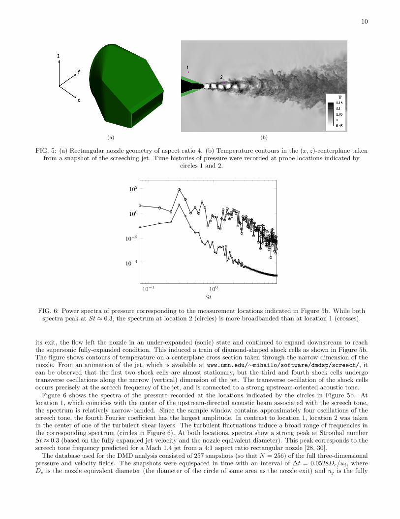
The supersonic jet used in this example was produced by a convergent rectangular nozzle of aspect ratio 4, preciselymatching the geometry of an experimental nozzle [29]; see Figure 5a for geometry. The entire flow inside, outside,

9

0 5 10 15 20 250

10

20

30

Nz

%Π

loss

FIG. 3: Performance loss % Πloss := 100√J(α)/J(0) of the optimal vector of amplitudes α resulting from the

sparsity-promoting DMD algorithm (with Nz DMD modes) for the Poiseuille flow example.

−0.6 −0.4 −0.2 0−1

−0.8

−0.6

−0.4

−0.2

Re (log (µi))

Im(l

og

(µi))

(a) Nz = 13

−0.6 −0.4 −0.2 0−1

−0.8

−0.6

−0.4

−0.2

Re (log (µi))

(b) Nz = 3

−0.6 −0.4 −0.2 0−1

−0.8

−0.6

−0.4

−0.2

Re (log (µi))

(c) Nz = 1

−1 −0.8 −0.6 −0.4 −0.20

5

10

15

Im (log (µi))

|αi|

(d) Nz = 13

−1 −0.8 −0.6 −0.4 −0.20

5

10

15

Im (log (µi))

(e) Nz = 3

−1 −0.8 −0.6 −0.4 −0.20

5

10

15

Im (log (µi))

(f) Nz = 1

FIG. 4: Eigenvalues of Fdmd (first row) and the absolute values of the DMD amplitudes αi (second row) for thePoiseuille flow example. The results are obtained using the standard DMD algorithm (circles) and the

sparsity-promoting DMD algorithm (crosses) with Nz DMD modes.

and downstream of the nozzle was simulated using the low-dissipation low-dispersion LES solver charles on anunstructured mesh with about 45 million control volumes. This simulation was a part of a sequence involving differentmesh resolutions, and it was validated against the experimental measurements [30].

The stagnation pressure and temperature inside the nozzle were set so that the jet Mach number Mj = 1.4 and thefully expanded jet temperature matched the ambient temperature. A rectangular nozzle whose interior cross sectionarea was decreasing monotonically from inlet to exit was used. Since the nozzle did not have a diverging section before

10

(a) (b)

FIG. 5: (a) Rectangular nozzle geometry of aspect ratio 4. (b) Temperature contours in the (x, z)-centerplane takenfrom a snapshot of the screeching jet. Time histories of pressure were recorded at probe locations indicated by

circles 1 and 2.

10−1 100

10−4

10−2

100

102

St

FIG. 6: Power spectra of pressure corresponding to the measurement locations indicated in Figure 5b. While bothspectra peak at St ≈ 0.3, the spectrum at location 2 (circles) is more broadbanded than at location 1 (crosses).

its exit, the flow left the nozzle in an under-expanded (sonic) state and continued to expand downstream to reachthe supersonic fully-expanded condition. This induced a train of diamond-shaped shock cells as shown in Figure 5b.The figure shows contours of temperature on a centerplane cross section taken through the narrow dimension of thenozzle. From an animation of the jet, which is available at www.umn.edu/∼mihailo/software/dmdsp/screech/, itcan be observed that the first two shock cells are almost stationary, but the third and fourth shock cells undergotransverse oscillations along the narrow (vertical) dimension of the jet. The transverse oscillation of the shock cellsoccurs precisely at the screech frequency of the jet, and is connected to a strong upstream-oriented acoustic tone.

Figure 6 shows the spectra of the pressure recorded at the locations indicated by the circles in Figure 5b. Atlocation 1, which coincides with the center of the upstream-directed acoustic beam associated with the screech tone,the spectrum is relatively narrow-banded. Since the sample window contains approximately four oscillations of thescreech tone, the fourth Fourier coefficient has the largest amplitude. In contrast to location 1, location 2 was takenin the center of one of the turbulent shear layers. The turbulent fluctuations induce a broad range of frequencies inthe corresponding spectrum (circles in Figure 6). At both locations, spectra show a strong peak at Strouhal numberSt ≈ 0.3 (based on the fully expanded jet velocity and the nozzle equivalent diameter). This peak corresponds to thescreech tone frequency predicted for a Mach 1.4 jet from a 4:1 aspect ratio rectangular nozzle [28, 30].

The database used for the DMD analysis consisted of 257 snapshots (so that N = 256) of the full three-dimensionalpressure and velocity fields. The snapshots were equispaced in time with an interval of ∆t = 0.0528De/uj , whereDe is the nozzle equivalent diameter (the diameter of the circle of same area as the nozzle exit) and uj is the fully

11

−2 0 20

1

2

3

·104

Im (log (µi))

|αi|

(a)

−0.8 −0.6 −0.4 −0.2 00

1

2

3

·104

Re (log (µi))

(b)

−2 · 10−2 −1 · 10−2 00

1,000

2,000

Re (log (µi))

(c)

FIG. 7: Dependence of the absolute value of the DMD amplitudes αi on (a) the frequency and (b,c) the real part ofthe corresponding DMD eigenvalues µi for the screeching jet example. Subfigure (c) represents a zoomed version of

subfigure (b) and it focuses on the amplitudes that correspond to lightly damped eigenvalues.

103 1040

100

200

γ

card

(α)

(a)

103 1040

5

10

15

γ

%Π

loss

(b)

FIG. 8: (a) The sparsity level card (α) and (b) the performance loss % Πloss := 100√J(α)/J(0) of the optimal

vector of amplitudes α resulting from the sparsity-promoting DMD algorithm for the screeching jet example.

expanded jet velocity. Although the computational domain for the LES extended approximately 32De downstreamof the nozzle exit, DMD was applied to a subdomain focusing on the shock cells within the jet’s potential core andthe surrounding acoustic field (this domain extends to 10De). This restriction reduced the number of cells from 45million to 8 million. In spite of this reduction, each snapshot required 256Mb of storage in double precision format. Tohandle such large matrices, DMD was implemented using a MapReduce framework so that the matrix could be storedand processed across several storage discs. In particular, the algorithm relied upon a MapReduce QR-factorization oftall-and-skinny matrices developed in [31].

Figure 7a illustrates the frequency dependence of the absolute value of the amplitudes of the DMD modes obtainedby solving the optimization problem (5). We note that it is not trivial to identify, by mere inspection, a subset of DMDmodes that has the strongest influence on the quality of the least-squares approximation. As shown in Figure 7b, thelargest amplitudes originate from eigenvalues that are strongly damped. In what follows, we demonstrate that keepingonly a subset of modes with largest amplitudes can lead to poor quality of approximation of numerically generatedsnapshots.

The sparsity level card (α) and the performance loss % Πloss := 100√J(α)/J(0) for the optimal vector of amplitudes

α resulting from the sparsity-promoting DMD algorithm are shown in Figure 8 as a function of the user-specifiedparameter γ (a measure of preference between approximation quality and solution sparsity). As expected, largervalues of γ encourage sparser solutions, at the expense of compromising quality of the least-squares approximation.The values of γ in Figure 8 are selected in such a way that γmin induces a dense vector α (with 256 non-zero elements),and γmax induces α with a single non-zero element.

12

−1 −0.5 0 0.5 1−1

−0.5

0

0.5

1

Re (µi)

Im(µ

i)

(a) Nz = 47

0.92 0.94 0.96 0.98 1−0.2

−0.1

0

0.1

0.2

Re (µi)

(b) Nz = 5

0.92 0.94 0.96 0.98 1−0.2

−0.1

0

0.1

0.2

Re (µi)

(c) Nz = 3

FIG. 9: Eigenvalues resulting from the standard DMD algorithm (circles) along with the subset of Nz eigenvaluesselected by the sparsity-promoting DMD algorithm (crosses) for the screeching jet example. In subfigures (b) and

(c), the dashed curves identify the unit circle.

−2 0 2101

102

103

104

Im (log (µi))

|αi|

(a) Nz = 47

−0.2 0 0.20

2,000

4,000

Im (log (µi))

(b) Nz = 5

−0.2 0 0.20

2,000

4,000

Im (log (µi))

(c) Nz = 3

FIG. 10: Dependence of the absolute value of the amplitudes αi on the frequency (imaginary part) of thecorresponding eigenvalues µi for the screeching jet example. The results are obtained using the standard DMD

algorithm (circles) and the sparsity-promoting DMD algorithm (crosses) with Nz DMD modes.

Eigenvalues resulting from the standard DMD algorithm (circles) along with the subset of Nz eigenvalues selectedby the sparsity-promoting DMD algorithm (crosses) are shown in Figure 9. Eigenvalues in the interior of the unit circleare strongly damped. Since a strongly damped mode influences only early stages of time evolution, the associatedamplitude |αi| can be large; see Figure 7b for an illustration. Rather than focusing only on the modes with largestamplitudes, the sparsity-promoting DMD identifies modes that have the strongest influence on the entire time historyof available snapshots. While the selection of the retained eigenvalues is non-trivial, it increasingly concentrates onthe low-frequency modes as Nz decreases. For Nz = 3, only the mean flow and one dominant frequency pair (thatcorresponds to the fundamental frequency of the screech tone) remain, while for Nz = 5 a second, lower frequency isidentified. In this low-Nz limit we do see that the sparsity-promoting DMD approximates the data sequence using themost prevalent structures. The corresponding amplitudes for the various truncations Nz are displayed in Figure 10.Again, as Nz decreases a concentration on low frequencies is observed. We also note that the amplitudes of theoriginal DMD modes do not provide sufficient guidance in reducing the full set of DMD modes to a few relevant ones.

Figure 11 illustrates performance of the sparsity-promoting DMD algorithm developed in this paper in terms ofthe number of identified structures. The performance is quantified by the Frobenius norm of the approximation errorbetween a low-dimensional representation and the full data sequence in fraction of the Frobenius norm of the fulldata sequence. As expected, the performance of our algorithm improves as the number of modes is increased. Forthe screeching jet example, the sparsity-promoting DMD with Nz = 3 gives St = 0.3104 which agrees well with thefrequency St = 0.3 measured from a sequence containing 10 times the number of snapshots.

Finally, Figure 12 visualizes the three-dimensional mode associated with the dominant frequency pair resulting

13

0 50 100 150 200 2500

5

10

15

Nz

%Π

loss

FIG. 11: The optimal performance loss, % Πloss := 100√J(α)/J(0), of the sparsity-promoting DMD algorithm for

the screeching jet example as a function of the number of retained modes.

FIG. 12: The three-dimensional DMD mode associated with the dominant frequency pair (that corresponds to thefundamental frequency of the screech tone, St ≈ 0.3). A red isosurface of perturbation pressure is shown together

with a blue isosurface of the perturbation dilatation. An animation of this flow field is available atwww.umn.edu/∼mihailo/software/dmdsp/screech/.

from the sparsity-promoting DMD algorithm. Isosurfaces of pressure and dilatation fluctuations are identified by redand blue colors, respectively. An animation of this mode reveals that the dilatation corresponds to a flapping modealong the narrow dimension of the jet; please see www.umn.edu/∼mihailo/software/dmdsp/screech/. As the shockcells oscillate transversely, they encroach into the jet shear layers, and compress the oncoming jet fluid in a regionwhere previously there was no compression. This time-periodic compression is connected to the upstream propagatingacoustic wave at the exterior of the jet. Furthermore, the animation of the DMD mode reveals that – close to thejet – the acoustic wave does not propagate smoothly in the upstream direction. Instead, the acoustic wave hops fromone spot of negative dilatation to the next as it proceeds upstream. As the oscillating shock cells penetrate into thejet shear layers, they are also rotated by the shear. When this happens, the outer tip of the shock cell sweeps fromdownstream to upstream, providing an impulse to the exterior acoustic perturbation which “kicks” it upstream to thenext shock cell.

14

(a) (b) (c)

FIG. 13: (a) Geometry of a flow between two cylinders along with the interrogation window where PIVmeasurements are taken. (b,c) Two representative snapshots of velocity vectors and vorticity contours, resulting

from time-resolved PIV measurements, illustrate the oscillatory motion of the exiting jet. See text for details on theexperimental parameters.

C. Flow through a cylinder bundle

Flow through cylinders in a bundle configuration is often encountered in the utility and energy conversion industry.Owing to their versatility and efficiency [32], cross-flow heat exchangers account for the vast majority of heat ex-changers in oil refining, process engineering, petroleum extraction, and power generation sectors. Consequently, evena modest improvement in their effectiveness and operational margins would have a significant impact on productionefficiency. In spite of their widespread use, the details of the flow (and heat transfer) through cylinder bundles arefar from fully understood, thereby making this type of flow, along with its simplified variants, the subject of activeresearch [33–36].

Vortex shedding and complex wake interactions can induce vibrations and structural resonances which, in turn,may result in fretting wear, collisional damage, material fatigue, creep, and ultimately in cracking. Even though theflow through a cylinder bundle is very complex, it is characterized by well-defined shedding frequencies [37]. Forsingle-row cylinders, only a few distinct frequencies are detected, while for more complex array configurations, amultitude of precise shedding frequencies are observed. The presence of distinct shedding frequencies makes this typeof flow well-suited for a decomposition of the flow fields into single-frequency modes.

In addition to the multiple-frequency behavior, a characteristic oscillatory pattern – labelled as a “flip-flop phe-nomenon” – is typically observed in the exit stream of the flow through cylinder bundles [38, 39]. The observedoscillatory pattern consists of a meta-stable deflection of the exiting jet off the centerline location. A statisticalanalysis of the velocity field in a cross-stream section shows a strongly bimodal distribution. Over a wide range ofReynolds numbers, the Strouhal number associated with the oscillation between these two states is approximatelyReynolds-number-independent. This flow feature can also be represented by a dynamic mode decomposition of theflow fields.

In this paper, we use a simplified geometric configuration that nonetheless inherits the main features from morecomplex settings, including the presence of multiple distinct frequencies and the flip-flop oscillations of the exit stream.In particular, we consider the flow passing between two cylinders; see Figure 13a for a sketch of the geometry. ThePIV interrogation window is positioned about one cylinder radius downstream of the passage. It measures 40.36mmin the streamwise and 32.08mm in the cross-stream direction. The flow field is resolved on a 63 × 79 measurementgrid, and two in-plane velocity components are recorded. The flow fields are represented in a fully time-resolvedmanner with 4ms between two consecutive PIV measurements. The inter-cylinder gap is 10.7mm and the jet passingbetween the two cylinders (of diameter 12mm) has a mean velocity of 0.663m/s. The resulting Reynolds number,

based on the volume flux velocity (Q = 18m3/h) and the cylinder diameter, is Re = 3000.Two representative snapshots resulting from a time-resolved flow field sequence display velocity vectors and contours

of the spanwise vorticity in Figure 13. The two flow fields are 0.28 s apart and show a downward (Figure 13b)and upward (Figure 13c) deflection of the jet exiting between the two cylinders. A time-sequence of flow fieldssubstantiates the existence of a low-frequency oscillation of the jet, which forms the basis of the afore-mentioned flip-flop phenomenon. A streamwise velocity signal has been extracted from the center of the experimental domain, anda subsequent spectral analysis of this signal reveals a distinct frequency of 7.81Hz which corresponds to a Strouhal

15

−3 −2 −1 0 1 2 30

50

100

Im (log (µi))

|αi|

(a)

−0.5 −0.4 −0.3 −0.2 −0.1 00

50

100

Re (log (µi))

(b)

FIG. 14: Dependence of the absolute value of the DMD amplitudes αi on (a) the frequency and (b) the real part ofthe corresponding DMD eigenvalues µi for the flow through a cylinder bundle.

−1 −0.5 0 0.5 1

−1

−0.5

0

0.5

1

Re (µi)

Im(µ

i)

(a) Nz = 21

0.9 0.92 0.94 0.96 0.98 1−0.4

−0.2

0

0.2

0.4

Re (µi)

(b) Nz = 5

0.9 0.92 0.94 0.96 0.98 1−0.4

−0.2

0

0.2

0.4

Re (µi)

(c) Nz = 3

FIG. 15: Eigenvalues resulting from the standard DMD algorithm (circles) along with the subset of Nz eigenvaluesselected by its sparsity-promoting variant (crosses) for the flow through a cylinder bundle. The dashed curves

identify the unit circle.

number St = 0.126 (based on the jet mean velocity and cylinder gap).Figure 14 shows the amplitudes of the DMD modes versus the identified frequencies and corresponding growth/decay

rates. These results were obtained using a database with N = 100 snapshots. As in the screeching jet example,strongly damped modes are characterized by large amplitudes, and a clear indication about the relative importance ofindividual DMD modes cannot be inferred from these two plots. Instead, we apply our sparsity-promoting frameworkto aid in the delineation of modes that contribute significantly to the data sequence and modes that capture onlytransient effects. By adjusting the user-specified parameter γ, we encourage solutions that consist of only a limitednumber of modes but still optimally represent the original data-sequence.

Figure 15 superimposes the eigenvalues resulting from the standard DMD algorithm (circles) and its sparsity-promoting variant (crosses). Even though the eigenvalues in the vicinity of the unit circle are associated with muchsmaller amplitudes than the strongly damped eigenvalues (that reside well within the unit circle), they are selected byour algorithm. As the sparsity parameter is increased and fewer eigenvalues are selected, a clustering of eigenvaluesat and near the point (1, 0) is observed; see Figure 15c.

A similar picture emerges from displaying the selected modes in the frequency-amplitude plane; see Figure 16.The sparsity-promoting DMD algorithm provides a rapid concentration on low-frequency modes, thereby eliminatingstructures with substantially larger amplitudes identified by the standard DMD algorithm. As the limit of only Nz = 3DMD modes is reached, the sparsity-promoting algorithm concentrates on frequencies that still optimally describe

16

−2 0 2

100

101

102

Im (log (µi))

|αi|

(a) Nz = 21

−0.4 −0.2 0 0.2 0.4

10

20

30

Im (log (µi))

(b) Nz = 5

−0.4 −0.2 0 0.2 0.4

10

20

30

Im (log (µi))

(c) Nz = 3

FIG. 16: Dependence of the absolute value of the amplitudes αi on the frequency (imaginary part) of thecorresponding eigenvalues µi for the flow through a cylinder bundle. The results are obtained using the standard

DMD algorithm (circles) and the sparsity-promoting DMD algorithm (crosses) with Nz DMD modes.

FIG. 17: Snapshot resulting from a sparse three-component (Nz = 3) representation of the full data sequence,visualized by velocity vectors and vorticity contours. An animation of this flow field is available at

www.umn.edu/∼mihailo/software/dmdsp/cylinder/.

the principal oscillatory components of the full data set. As evident from Figure 16c, for Nz = 3 the last oscillatoryrepresentation is characterized by Im (log(µi)) ≈ 0.201 (which corresponds to a frequency of 7.99Hz and a Strouhalnumber of St = 0.129). This frequency is in good agreement with the frequency identified by the aforementionedpoint measurements of the streamwise velocity. The flow field associated with the three-term (Nz = 3) representationof the data sequence is displayed in Figure 17; it consists of a deflected jet and strong vortical components off thesymmetry axis. An animation of this flow field, available at www.umn.edu/∼mihailo/software/dmdsp/cylinder/,has been obtained using the identified and selected frequency (7.99Hz) and it reproduces the main features of the fulldata sequence, i.e., the lateral swaying of the jet under the influence of the wake vortices of the two cylinders.

The sparse approximation of the full data-sequence focuses on the most relevant structures by removing large-amplitude but transient flow features and it results in progressively larger residuals as the sparsity is enhanced.This inherent trade-off between a more compact data representation and the quality of approximation compared tothe original data sequence is depicted in Figure 18. In contrast to the channel flow and screeching jet examples,the sparsity-promoting version of the DMD-algorithm displays higher performance degradation. This behavior mayperhaps be attributed to the presence of unstructured measurement noise in the experimental dataset for a jet passingbetween two cylinders.

17

0 20 40 60 80 1000

20

40

60

Nz

%Π

loss

FIG. 18: The optimal performance loss, % Πloss := 100√J(α)/J(0), of the sparsity-promoting DMD algorithm for

the flow through a cylinder bundle as a function of the number of retained modes.

V. CONCLUDING REMARKS

We have introduced an extension of the standard DMD algorithm that addresses the reduction in dimensionalityof the full rank decomposition. This reduction is accomplished by a sparsity-promoting procedure which augmentsthe standard least-squares optimization problem by a term that penalizes the `1-norm of the vector of unknownamplitudes. A user-specified regularization parameter balances the trade-off between the quality of approximationand the number of retained DMD modes. The sparsity-promoting DMD algorithm thus selects specific dynamic modes(along with their associated temporal frequencies and growth/decay rates) which exhibit the strongest contributionto a representation of the original data sequence over the considered time interval.

The `1-regularized least-squares problem can be formulated as a convex optimization problem for which the alter-nating direction method of multipliers (ADMM) provides an efficient tool for computing the globally optimal solution.ADMM is an iterative method that alternates between minimization of the least-squares residual and sparsity en-hancement. We have shown that the least-squares minimization step amounts to solving an unconstrained regularizedquadratic program and that sparsity is promoted through the application of a soft-thresholding operator. After adesirable tradeoff between the quality of approximation and the number of DMD modes has been accomplished, wefix the sparsity structure and compute the optimal amplitudes of the retained dynamic modes.

The sparsity-promoting dynamic mode decomposition has been applied to three examples. The linearized planePoiseuille flow at a supercritical Reynolds number was used to showcase the algorithm on a canonical flow configuration;the sparsity-promoting DMD extracted modal contributions from each of the familiar eigenvalue branches until onlythe exponentially growing TS wave was retained in the limit of maximal sparsity. For the unstructured large-eddysimulation of a supersonic screeching jet, the sparsity-promoting DMD algorithm successfully and efficiently identifiedthe screech frequency and the associated flow fields; dynamic modes with large amplitudes and substantial decayrates, representing transient flow features, have been eliminated as our emphasis on sparsity increased. Finally, fortwo-dimensional time-resolved PIV measurements of a jet passing between two cylinders, the prevailing Strouhalnumber has been identified by the dynamic mode decomposition, and the sparsity-promoting algorithm effectivelydifferentiated the dominant flow structures from less relevant flow phenomena embedded in the full data sequence.

The developed method builds on recent attempts at optimizing the standard dynamic mode decomposition [14–16] and at providing a framework for the automated detection of a few pertinent modal flow features. While theseefforts resulted in complex or nearly intractable non-convex optimization problems, the sparsity-promoting DMDalgorithm provides an efficient paradigm for detection and extraction of a limited subset of flow features that optimallyapproximate the original data sequence. Furthermore, in contrast to the aforementioned attempts, our approachregularizes the least-squares deviation between the matrix of snapshots and the linear combination of DMD modeswith a term that penalizes the `1-norm of the vector of unknown DMD amplitudes. While the former term dependsboth on the problem data and on the optimization variable, the latter term is problem-data-independent; its primarypurpose is to enhance desirable features in the solution to the resulting regularized optimization problem. We notethat regularization may be of essence in the situations where the problem data is corrupted by noise or containsnumerical or experimental outliers. In the absence of regularization, the predictive capability of low-dimensional

18

models resulting from corrupted or incomplete snapshots may be significantly diminished. Exploration of differenttypes of regularization penalties, that are well-suited for the problems in fluid mechanics, is an effort worth pursuing.

The developed algorithm has shown its value on the numerical and experimental snapshot sequences considered inthis paper. It is expected that the sparsity-promoting dynamic mode decomposition will become a valuable tool inthe quantitative analysis of high-dimensional datasets, in the interpretation of identified dynamic modes, and in theeduction of relevant physical mechanisms.

SUPPLEMENTARY MATERIAL

Additional information about the examples considered in this paper, along with Matlab source codes and problemdata, can be found at www.umn.edu/∼mihailo/software/dmdsp/.

ACKNOWLEDGMENTS

The authors gratefully acknowledge Prof. Parviz Moin for his encouragement to pursue this effort during the 2012Center for Turbulence Research Summer Program at Stanford University. Supported in part by Stanford Universityand NASA Ames Research Center, and by the University of Minnesota Initiative for Renewable Energy and theEnvironment under Early Career Award RC-0014-11. The time-resolved PIV measurements of a jet passing betweentwo cylinders were provided by Electricite de France (EdF).

Appendix A: An alternative formulation of (5)

We show that the objective function J(α) in (5),

J(α) = ‖G − LDαR‖2F , (A1)

with

G := ΣV ∗, L := Y, Dα := diag {α}, R := Vand,

can be equivalently represented as (6). The equivalence between (A1) and (6) can be established through a sequenceof straightforward algebraic manipulations in conjunction with the repeated use of the following properties of thematrix trace:

P1: Commutativity invariance,

trace (AB) = trace (BA) ;

P2: A product between a matrix Q and a diagonal matrix Dα := diag {α},

trace (QDα) = (diag {Q})Tα =(

diag {Q})∗α;

P3: For vectors α ∈ Cn and β ∈ Cm and matrices A,B ∈ Cm×n,

trace(D∗β ADαB

T)

= β∗(A ◦B)α.

Now, a repeated use of the matrix trace commutativity invariance property P1 leads to

J(α) = ‖G − LDαR‖2F= trace

((G − LDαR)

∗(G − LDαR)

)= trace (D∗α (L∗L)Dα (RR∗) − QDα − Q∗D∗α + G∗G) ,

and the equivalence between (A1) and (6) follows from P2 and P3.

19

Appendix B: α- and β-minimization steps in ADMM

We exploit the respective structures of the functions J and g in (10) and show that the α-minimization step amountsto solving an unconstrained regularized quadratic program and that the β-minimization step amounts to an opportuneuse of the soft thresholding operator.

• α-minimization step: Completion of squares with respect to α in the augmented Lagrangian Lρ can be usedto show that the α-minimization step (12a) is equivalent to

minimizeα

J(α) +ρ

2‖α − uk‖22,

where

uk = βk − (1/ρ)λk.

Now, the definition (6) of J leads to the unconstrained quadratic programming problem

minimizeα

α∗(P + (ρ/2) I)α −(q + (ρ/2)uk

)∗α − α∗

(q + (ρ/2)uk

)+ s + ρ ‖uk‖22,

whose solution is determined by

αk+1 = (P + (ρ/2) I)−1 (

q + (ρ/2)uk).

• β-minimization step: The completion of squares with respect to β in the augmented Lagrangian Lρ can beused to show that the β-minimization step (12b) is equivalent to

minimizeβ

γ g(β) +ρ

2‖β − vk‖22,

where

vk = αk+1 + (1/ρ)λk.

It is a standard fact that the solution to this optimization problem is determined by

βk+1i = Sκ(vki ), κ = γ/ρ,

where Sκ(·) denotes the soft thresholding operator

Sκ(vki ) =

vki − κ, vki > κ

0, vki ∈ [−κ, κ]

vki + κ, vki < −κ.

Appendix C: An efficient algorithm for solving (9)

From Appendix A it follows that finding the solution to (9) amounts to solving the following equality-constrainedquadratic programming problem

minimizeα

J(α) = α∗P α − q∗α − α∗q + s

subject to ET α = 0.

It is a standard fact that the variation of the Lagrangian

L(α, ν) = J(α) + ν∗ETα +(ETα

)∗ν,

with respect to α and the vector of Lagrange multipliers ν can be used to obtain the conditions for optimality of L,[P E

ET 0

] [α

ν

]=

[q

0

].

20

The optimal sparse vector of amplitudes, αsp, is then determined by

αsp =[I 0

] [ P E

ET 0

]−1 [q

0

].

[1] J. Lumley, Stochastic Tools in Turbulence. Dover Publications, 2007.[2] L. Sirovich, “Turbulence and the dynamics of coherent structures. Part I: Coherent structures,” Quart. Appl. Math., vol.

45(3), pp. 561–571, 1987.[3] D. Sipp, O. Marquet, P. Meliga, and A. Barbagallo, “Dynamics and control of global instabilities in open flows: a linearized

approach,” Appl. Mech. Rev., vol. 63, p. 030801, 2010.[4] B. Moore, “Principal component analysis in linear systems: controllability, observability and model reduction,” IEEE

Trans. Automat. Control, vol. AC-26(1), 1981.[5] C. Rowley, “Model reduction for fluids using balanced proper orthogonal decomposition,” Int. J. Bifurcation Chaos, vol. 15,

pp. 997–1013, 2005.[6] I. Mezic, “Spectral properties of dynamical systems, model reduction and decompositions,” Nonlinear Dynamics, vol. 41,

no. 1, pp. 309–325, 2005.[7] C. Rowley, I. Mezic, S. Bagheri, P. Schlatter, and D. Henningson, “Spectral analysis of nonlinear flows,” J. Fluid Mech.,

vol. 641, pp. 115–127, 2009.[8] I. Mezic, “Analysis of fluid flows via spectral properties of Koopman operator,” Ann. Rev. Fluid Mech., vol. 45, no. 1, pp.

357–378, 2013.[9] P. J. Schmid, “Dynamic mode decomposition of numerical and experimental data,” J. Fluid Mech., vol. 656, pp. 5–28,

2010.[10] L. N. Trefethen, A. E. Trefethen, S. C. Reddy, and T. A. Driscoll, “Hydrodynamic stability without eigenvalues,” Science,

vol. 261, pp. 578–584, 1993.[11] M. R. Jovanovic and B. Bamieh, “Componentwise energy amplification in channel flows,” J. Fluid Mech., vol. 534, pp.

145–183, July 2005.[12] P. J. Schmid, “Nonmodal stability theory,” Annu. Rev. Fluid Mech., vol. 39, pp. 129–162, 2007.[13] S. Bagheri, “Koopman-mode decomposition of the cylinder wake,” J. Fluid Mech., vol. 726, pp. 596–623, 2013.[14] K. K. Chen, J. H. Tu, and C. W. Rowley, “Variants of dynamic mode decomposition: boundary condition, Koopman, and

Fourier analyses,” J. Nonlinear Sci., vol. 22, no. 6, pp. 887–915, 2012.[15] P. J. Goulart, A. Wynn, and D. Pearson, “Optimal mode decomposition for high dimensional systems,” in 51st IEEE

Conference on Decision and Control, 2012, pp. 4965–4970.[16] A. Wynn, D. Pearson, B. Ganapathisubramani, and P. J. Goulart, “Optimal mode decomposition for unsteady flows,” J.

Fluid Mech., 2013, to appear.[17] S. Boyd and L. Vandenberghe, Convex optimization. Cambridge University Press, 2004.[18] E. J. Candes, J. Romberg, and T. Tao, “Robust uncertainty principles: Exact signal reconstruction from highly incomplete

frequency information,” IEEE Trans. Inf. Theory, vol. 52, no. 2, pp. 489–509, 2006.[19] D. L. Donoho, “Compressed sensing,” IEEE Trans. Inf. Theory, vol. 52, no. 4, pp. 1289–1306, 2006.[20] E. J. Candes and T. Tao, “Near optimal signal recovery from random projections: Universal encoding strategies?” IEEE

Trans. Inf. Theory, vol. 52, no. 12, pp. 5406–5425, 2006.[21] E. J. Candes, M. B. Wakin, and S. P. Boyd, “Enhancing sparsity by reweighted `1 minimization,” J. Fourier Anal. Appl,

vol. 14, pp. 877–905, 2008.[22] T. Hastie, R. Tibshirani, and J. Friedman, The elements of statistical learning. Springer, 2009.[23] S. Boyd, N. Parikh, E. Chu, B. Peleato, and J. Eckstein, “Distributed optimization and statistical learning via the

alternating direction method of multipliers,” Foundations and Trends in Machine Learning, vol. 3, no. 1, pp. 1–124, 2011.[24] F. Lin, M. Fardad, and M. R. Jovanovic, “Design of optimal sparse feedback gains via the alternating direction method of

multipliers,” IEEE Trans. Automat. Control, vol. 58, no. 9, pp. 2426–2431, 2013.[25] M. Grant and S. Boyd, “CVX: Matlab software for disciplined convex programming, version 2.0 beta,” http://cvxr.com/

cvx, 2012.[26] P. J. Schmid and D. S. Henningson, Stability and Transition in Shear Flows. Springer-Verlag, 2001.[27] J. A. C. Weideman and S. C. Reddy, “A MATLAB differentiation matrix suite,” ACM Transactions on Mathematical

Software, vol. 26, no. 4, pp. 465–519, December 2000.[28] C. K. W. Tam, “Supersonic jet noise,” Annu. Rev. Fluid Mech., vol. 27, pp. 17–43, 1995.[29] F. C. Frate and J. E. Bridges, “Extensible rectangular nozzle model system,” AIAA Paper 2011-975, 2011.[30] J. W. Nichols, F. E. Ham, and S. K. Lele, “High-fidelity large-eddy simulation for supersonic rectangular jet noise predic-

tion,” AIAA Paper 2011-2919, 2011.[31] P. G. Constantine and D. F. Gleich, “Tall and skinny QR factorizations in MapReduce architectures,” in Proceedings of

the 2nd international workshop on MapReduce and its applications, 2011, pp. 43–50.[32] S. Kakac and H. Liu, Heat Exchangers: Selection, Rating and Thermal Design. CRC Press, 1997.

21

[33] P. Rollet-Miet, D. Laurence, and J. Ferziger, “LES and RANS of turbulent flow in tube bundles,” Int. J. Heat and FluidFlow, vol. 20, pp. 241–254, 1999.

[34] D. Sumner, S. Price, and M. Paidoussis, “Flow-pattern identification for two staggered circular cylinders in cross-flow,” J.Fluid Mech., vol. 411, pp. 263–303, 2000.

[35] S. Benhamadouche and D. Laurence, “LES, coarse LES, and transient RANS comparisons on the flow across a tubebundle,” Int. J. Heat and Fluid Flow, vol. 24, pp. 470–479, 2003.

[36] C. Moulinec, M. Pourquie, B. Boersma, T. Buchal, and F. Nieuwstadt, “Direct numerical simulation on a Cartesian meshof the flow through a tube bundle,” Int. J. Comp. Fluid Dyn., vol. 18, pp. 1–14, 2004.

[37] C. Liang and G. Papadakis, “Large eddy simulation of cross-flow through a staggered tube bundle at subcritical Reynoldsnumber,” J. Fluids Struct., vol. 23, pp. 1215–1230, 2007.

[38] O. Simonin and M. Barcouda, “Measurements and prediction of turbulent flow entering a staggered tube bundle,” inProceedings of the 4th International Symposium on Applications of Laser Anemometry to Fluid Mechanics, Lisbon, 1988,p. 5.23.

[39] Y. Hassan and H. Barsamian, “Turbulence simulation in tube bundle geometries using the dynamic subgrid-scale model,”Nuclear Techn. J., vol. 128, pp. 58–74, 1999.