journal of applied functional analysis - eudoxus … · the purpose of the "journal of applied...
TRANSCRIPT
Volume 7, Numbers 1-2 January-April 2012 ISSN:1559-1948 (PRINT), 1559-1956 (ONLINE) EUDOXUS PRESS,LLC
JOURNAL OF APPLIED FUNCTIONAL ANALYSIS
1
SCOPE AND PRICES OF
JOURNAL OF APPLIED FUNCTIONAL ANALYSIS A quartely international publication of EUDOXUS PRESS,LLC ISSN:1559-1948(PRINT),1559-1956(ONLINE) Editor in Chief: George Anastassiou Department of Mathematical Sciences The University of Memphis Memphis, TN 38152,USA E mail: [email protected] Assistant to the Editor:Dr.Razvan Mezei,Lander University,SC 29649, USA. -------------------------------------------------------------------------------- The purpose of the "Journal of Applied Functional Analysis"(JAFA) is to publish high quality original research articles, survey articles and book reviews from all subareas of Applied Functional Analysis in the broadest form plus from its applications and its connections to other topics of Mathematical Sciences. A sample list of connected mathematical areas with this publication includes but is not restricted to: Approximation Theory, Inequalities, Probability in Analysis, Wavelet Theory, Neural Networks, Fractional Analysis, Applied Functional Analysis and Applications, Signal Theory, Computational Real and Complex Analysis and Measure Theory, Sampling Theory, Semigroups of Operators, Positive Operators, ODEs, PDEs, Difference Equations, Rearrangements, Numerical Functional Analysis, Integral equations, Optimization Theory of all kinds, Operator Theory, Control Theory, Banach Spaces, Evolution Equations, Information Theory, Numerical Analysis, Stochastics, Applied Fourier Analysis, Matrix Theory, Mathematical Physics, Mathematical Geophysics, Fluid Dynamics, Quantum Theory. Interpolation in all forms, Computer Aided Geometric Design, Algorithms, Fuzzyness, Learning Theory, Splines, Mathematical Biology, Nonlinear Functional Analysis, Variational Inequalities, Nonlinear Ergodic Theory, Functional Equations, Function Spaces, Harmonic Analysis, Extrapolation Theory, Fourier Analysis, Inverse Problems, Operator Equations, Image Processing, Nonlinear Operators, Stochastic Processes, Mathematical Finance and Economics, Special Functions, Quadrature, Orthogonal Polynomials, Asymptotics, Symbolic and Umbral Calculus, Integral and Discrete Transforms, Chaos and Bifurcation, Nonlinear Dynamics, Solid Mechanics, Functional Calculus, Chebyshev Systems. Also are included combinations of the above topics. Working with Applied Functional Analysis Methods has become a main trend in recent years, so we can understand better and deeper and solve important problems of our real and scientific world. JAFA is a peer-reviewed International Quarterly Journal published by Eudoxus Press,LLC. We are calling for high quality papers for possible publication. The contributor should submit the contribution to the EDITOR in CHIEF in TEX or LATEX double spaced and ten point type size, also in PDF format. Article should be sent ONLY by E-MAIL [See: Instructions to Contributors] Journal of Applied Functional Analysis(JAFA)
is published in January,April,July and October of each year by
2

EUDOXUS PRESS,LLC, 1424 Beaver Trail Drive,Cordova,TN38016,USA, Tel.001-901-751-3553 [email protected] http://www.EudoxusPress.com visit also http://www.msci.memphis.edu/~ganastss/jafa. Webmaster:Ray Clapsadle Annual Subscription Current Prices:For USA and Canada,Institutional:Print $400,Electronic $250,Print and Electronic $450.Individual:Print $ 150, Electronic $80,Print &Electronic $200.For any other part of the world add $50 more to the above prices for Print. Single article PDF file for individual $15.Single issue in PDF form for individual $60. No credit card payments.Only certified check,money order or international check in US dollars are acceptable. Combination orders of any two from JoCAAA,JCAAM,JAFA receive 25% discount,all three receive 30% discount. Copyright©2012 by Eudoxus Press,LLC all rights reserved.JAFA is printed in USA. JAFA is reviewed and abstracted by AMS Mathematical Reviews,MATHSCI,and Zentralblaat MATH. It is strictly prohibited the reproduction and transmission of any part of JAFA and in any form and by any means without the written permission of the publisher.It is only allowed to educators to Xerox articles for educational purposes.The publisher assumes no responsibility for the content of published papers. JAFA IS A JOURNAL OF RAPID PUBLICATION
3
Journal of Applied Functional Analysis Editorial Board
Associate Editors
Editor in-Chief: George A.Anastassiou Department of Mathematical Sciences The University of Memphis Memphis,TN 38152,USA 901-678-3144 office 901-678-2482 secretary 901-751-3553 home 901-678-2480 Fax [email protected] Approximation Theory,Inequalities,Probability, Wavelet,Neural Networks,Fractional Calculus Associate Editors: 1) Francesco Altomare Dipartimento di Matematica Universita' di Bari Via E.Orabona,4 70125 Bari,ITALY Tel+39-080-5442690 office +39-080-3944046 home +39-080-5963612 Fax [email protected] Approximation Theory, Functional Analysis, Semigroups and Partial Differential Equations, Positive Operators. 2) Angelo Alvino Dipartimento di Matematica e Applicazioni "R.Caccioppoli" Complesso Universitario Monte S. Angelo Via Cintia 80126 Napoli,ITALY +39(0)81 675680 [email protected], [email protected] Rearrengements, Partial Differential Equations. 3) Catalin Badea UFR Mathematiques,Bat.M2, Universite de Lille1 Cite Scientifique F-59655 Villeneuve d'Ascq,France
23) Nikolaos B.Karayiannis Department of Electrical and Computer Engineering N308 Engineering Building 1 University of Houston Houston,Texas 77204-4005 USA Tel (713) 743-4436 Fax (713) 743-4444 [email protected] [email protected] Neural Network Models, Learning Neuro-Fuzzy Systems. 24) Theodore Kilgore Department of Mathematics Auburn University 221 Parker Hall, Auburn University Alabama 36849,USA Tel (334) 844-4620 Fax (334) 844-6555 [email protected] Real Analysis,Approximation Theory, Computational Algorithms. 25) Jong Kyu Kim Department of Mathematics Kyungnam University Masan Kyungnam,631-701,Korea Tel 82-(55)-249-2211 Fax 82-(55)-243-8609 [email protected] Nonlinear Functional Analysis,Variational Inequalities,Nonlinear Ergodic Theory, ODE,PDE,Functional Equations. 26) Robert Kozma Department of Mathematical Sciences The University of Memphis Memphis, TN 38152 USA [email protected] Neural Networks, Reproducing Kernel Hilbert Spaces, Neural Perculation Theory 27) Miroslav Krbec
4

Tel.(+33)(0)3.20.43.42.18 Fax (+33)(0)3.20.43.43.02 [email protected] Approximation Theory, Functional Analysis, Operator Theory. 4) Erik J.Balder Mathematical Institute Universiteit Utrecht P.O.Box 80 010 3508 TA UTRECHT The Netherlands Tel.+31 30 2531458 Fax+31 30 2518394 [email protected] Control Theory, Optimization, Convex Analysis, Measure Theory, Applications to Mathematical Economics and Decision Theory. 5) Carlo Bardaro Dipartimento di Matematica e Informatica Universita di Perugia Via Vanvitelli 1 06123 Perugia, ITALY TEL+390755853822 +390755855034 FAX+390755855024 E-mail [email protected] Web site: http://www.unipg.it/~bardaro/ Functional Analysis and Approximation Theory, Signal Analysis, Measure Theory, Real Analysis. 6) Heinrich Begehr Freie Universitaet Berlin I. Mathematisches Institut, FU Berlin, Arnimallee 3,D 14195 Berlin Germany, Tel. +49-30-83875436, office +49-30-83875374, Secretary Fax +49-30-83875403 [email protected] Complex and Functional Analytic Methods in PDEs, Complex Analysis, History of Mathematics. 7) Fernando Bombal Departamento de Analisis Matematico Universidad Complutense Plaza de Ciencias,3 28040 Madrid, SPAIN Tel. +34 91 394 5020 Fax +34 91 394 4726 [email protected]
Mathematical Institute Academy of Sciences of Czech Republic Zitna 25 CZ-115 67 Praha 1 Czech Republic Tel +420 222 090 743 Fax +420 222 211 638 [email protected] Function spaces,Real Analysis,Harmonic Analysis,Interpolation and Extrapolation Theory,Fourier Analysis. 28) V. Lakshmikantham Department of Mathematical Sciences Florida Institute of Technology Melbourne, FL 32901 e-mail: [email protected] Ordinary and Partial Differential Equations, Hybrid Systems, Nonlinear Analysis 29) Peter M.Maass Center for Industrial Mathematics Universitaet Bremen Bibliotheksstr.1, MZH 2250, 28359 Bremen Germany Tel +49 421 218 9497 Fax +49 421 218 9562 [email protected] Inverse problems,Wavelet Analysis and Operator Equations,Signal and Image Processing. 30) Julian Musielak Faculty of Mathematics and Computer Science Adam Mickiewicz University Ul.Umultowska 87 61-614 Poznan Poland Tel (48-61) 829 54 71 Fax (48-61) 829 53 15 [email protected] Functional Analysis, Function Spaces, Approximation Theory,Nonlinear Operators. 31) Gaston M. N'Guerekata Department of Mathematics Morgan State University Baltimore, MD 21251, USA tel:: 1-443-885-4373 Fax 1-443-885-8216 Gaston.N'[email protected] Nonlinear Evolution Equations, Abstract Harmonic Analysis, Fractional Differential Equations,
5

Operators on Banach spaces, Tensor products of Banach spaces, Polymeasures, Function spaces. 8) Michele Campiti Department of Mathematics "E.De Giorgi" University of Lecce P.O. Box 193 Lecce,ITALY Tel. +39 0832 297 432 Fax +39 0832 297 594 [email protected] Approximation Theory, Semigroup Theory, Evolution problems, Differential Operators. 9)Domenico Candeloro Dipartimento di Matematica e Informatica Universita degli Studi di Perugia Via Vanvitelli 1 06123 Perugia ITALY Tel +39(0)75 5855038 +39(0)75 5853822, +39(0)744 492936 Fax +39(0)75 5855024 [email protected] Functional Analysis, Function spaces, Measure and Integration Theory in Riesz spaces. 10) Pietro Cerone School of Computer Science and Mathematics, Faculty of Science, Engineering and Technology, Victoria University P.O.14428,MCMC Melbourne,VIC 8001,AUSTRALIA Tel +613 9688 4689 Fax +613 9688 4050 [email protected] Approximations, Inequalities, Measure/Information Theory, Numerical Analysis, Special Functions. 11)Michael Maurice Dodson Department of Mathematics University of York, York YO10 5DD, UK Tel +44 1904 433098 Fax +44 1904 433071 [email protected] Harmonic Analysis and Applications to Signal Theory,Number Theory and Dynamical Systems.
Almost Periodicity & Almost Automorphy. 32) Vassilis Papanicolaou Department of Mathematics National Technical University of Athens Zografou campus, 157 80 Athens, Greece tel:: +30(210) 772 1722 Fax +30(210) 772 1775 [email protected] Partial Differential Equations, Probability. 33) Pier Luigi Papini Dipartimento di Matematica Piazza di Porta S.Donato 5 40126 Bologna ITALY Fax +39(0)51 582528 [email protected] Functional Analysis, Banach spaces, Approximation Theory. 34) Svetlozar T.Rachev Chair of Econometrics,Statistics and Mathematical Finance School of Economics and Business Engineering University of Karlsruhe Kollegium am Schloss, Bau II,20.12, R210 Postfach 6980, D-76128, Karlsruhe,GERMANY. Tel +49-721-608-7535, +49-721-608-2042(s) Fax +49-721-608-3811 [email protected] Second Affiliation: Dept.of Statistics and Applied Probability University of California at Santa Barbara [email protected] Probability,Stochastic Processes and Statistics,Financial Mathematics, Mathematical Economics. 35) Paolo Emilio Ricci Department of Mathematics Rome University "La Sapienza" P.le A.Moro,2-00185 Rome,ITALY Tel ++3906-49913201 office ++3906-87136448 home Fax ++3906-44701007 [email protected] [email protected] Special Functions, Integral and Discrete
6
12) Sever S.Dragomir School of Computer Science and Mathematics, Victoria University, PO Box 14428, Melbourne City, MC 8001,AUSTRALIA Tel. +61 3 9688 4437 Fax +61 3 9688 4050 [email protected] Inequalities,Functional Analysis, Numerical Analysis, Approximations, Information Theory, Stochastics. 13) Paulo J.S.G.Ferreira Department of Electronica e Telecomunicacoes/IEETA Universidade de Aveiro 3810-193 Aveiro PORTUGAL Tel +351-234-370-503 Fax +351-234-370-545 [email protected] Sampling and Signal Theory, Approximations, Applied Fourier Analysis, Wavelet, Matrix Theory. 14) Gisele Ruiz Goldstein Department of Mathematical Sciences The University of Memphis Memphis,TN 38152,USA. Tel 901-678-2513 Fax 901-678-2480 [email protected] PDEs, Mathematical Physics, Mathematical Geophysics. 15) Jerome A.Goldstein Department of Mathematical Sciences The University of Memphis Memphis,TN 38152,USA Tel 901-678-2484 Fax 901-678-2480 [email protected] PDEs,Semigroups of Operators, Fluid Dynamics,Quantum Theory. 16) Heiner Gonska Institute of Mathematics University of Duisburg-Essen Lotharstrasse 65 D-47048 Duisburg Germany Tel +49 203 379 3542 Fax +49 203 379 1845 [email protected] Approximation and Interpolation Theory,
Transforms, Symbolic and Umbral Calculus, ODE, PDE,Asymptotics, Quadrature, Matrix Analysis. 36) Silvia Romanelli Dipartimento di Matematica Universita' di Bari Via E.Orabona 4 70125 Bari, ITALY. Tel (INT 0039)-080-544-2668 office 080-524-4476 home 340-6644186 mobile Fax -080-596-3612 Dept. [email protected] PDEs and Applications to Biology and Finance, Semigroups of Operators. 37) Boris Shekhtman Department of Mathematics University of South Florida Tampa, FL 33620,USA Tel 813-974-9710 [email protected] Approximation Theory, Banach spaces, Classical Analysis. 38) Rudolf Stens Lehrstuhl A fur Mathematik RWTH Aachen 52056 Aachen Germany Tel ++49 241 8094532 Fax ++49 241 8092212 [email protected] Approximation Theory, Fourier Analysis, Harmonic Analysis, Sampling Theory. 39) Juan J.Trujillo University of La Laguna Departamento de Analisis Matematico C/Astr.Fco.Sanchez s/n 38271.LaLaguna.Tenerife. SPAIN Tel/Fax 34-922-318209 [email protected] Fractional: Differential Equations-Operators- Fourier Transforms, Special functions, Approximations,and Applications. 40) Tamaz Vashakmadze I.Vekua Institute of Applied Mathematics Tbilisi State University, 2 University St. , 380043,Tbilisi, 43, GEORGIA. Tel (+99532) 30 30 40 office
7
Computer Aided Geometric Design, Algorithms. 17) Karlheinz Groechenig Institute of Biomathematics and Biometry, GSF-National Research Center for Environment and Health Ingolstaedter Landstrasse 1 D-85764 Neuherberg,Germany. Tel 49-(0)-89-3187-2333 Fax 49-(0)-89-3187-3369 [email protected] Time-Frequency Analysis, Sampling Theory, Banach spaces and Applications, Frame Theory. 18) Vijay Gupta School of Applied Sciences Netaji Subhas Institute of Technology Sector 3 Dwarka New Delhi 110075, India e-mail: [email protected]; [email protected] Approximation Theory 19) Weimin Han Department of Mathematics University of Iowa Iowa City, IA 52242-1419 319-335-0770 e-mail: [email protected] Numerical analysis, Finite element method, Numerical PDE, Variational inequalities, Computational mechanics 20) Tian-Xiao He Department of Mathematics and Computer Science P.O.Box 2900,Illinois Wesleyan University Bloomington,IL 61702-2900,USA Tel (309)556-3089 Fax (309)556-3864 [email protected] Approximations,Wavelet, Integration Theory, Numerical Analysis, Analytic Combinatorics. 21) Don Hong Department of Mathematical Sciences Middle Tennessee State University 1301 East Main St. Room 0269, Blgd KOM Murfreesboro, TN 37132-0001 Tel (615) 904-8339 [email protected] Approximation Theory,Splines,Wavelet, Stochastics, Mathematical Biology Theory.
(+99532) 30 47 84 office (+99532) 23 09 18 home [email protected] [email protected] Applied Functional Analysis, Numerical Analysis, Splines, Solid Mechanics. 41) Ram Verma International Publications 5066 Jamieson Drive, Suite B-9, Toledo, Ohio 43613,USA. [email protected] [email protected] Applied Nonlinear Analysis, Numerical Analysis, Variational Inequalities, Optimization Theory, Computational Mathematics, Operator Theory. 42) Gianluca Vinti Dipartimento di Matematica e Informatica Universita di Perugia Via Vanvitelli 1 06123 Perugia ITALY Tel +39(0) 75 585 3822, +39(0) 75 585 5032 Fax +39 (0) 75 585 3822 [email protected] Integral Operators, Function Spaces, Approximation Theory, Signal Analysis. 43) Ursula Westphal Institut Fuer Mathematik B Universitaet Hannover Welfengarten 1 30167 Hannover,GERMANY Tel (+49) 511 762 3225 Fax (+49) 511 762 3518 [email protected] Semigroups and Groups of Operators, Functional Calculus, Fractional Calculus, Abstract and Classical Approximation Theory, Interpolation of Normed spaces. 44) Ronald R.Yager Machine Intelligence Institute Iona College New Rochelle,NY 10801,USA Tel (212) 249-2047 Fax(212) 249-1689 [email protected] [email protected] Fuzzy Mathematics, Neural Networks, Reasoning, Artificial Intelligence, Computer Science.
8

22) Hubertus Th. Jongen Department of Mathematics RWTH Aachen Templergraben 55 52056 Aachen Germany Tel +49 241 8094540 Fax +49 241 8092390 [email protected] Parametric Optimization, Nonconvex Optimization, Global Optimization.
45) Richard A. Zalik Department of Mathematics Auburn University Auburn University,AL 36849-5310 USA. Tel 334-844-6557 office 678-642-8703 home Fax 334-844-6555 [email protected] Approximation Theory,Chebychev Systems, Wavelet Theory.
9

Instructions to Contributors
Journal of Applied Functional Analysis A quartely international publication of Eudoxus Press, LLC, of TN.
Editor in Chief: George Anastassiou
Department of Mathematical Sciences University of Memphis
Memphis, TN 38152-3240, U.S.A.
1. Manuscripts files in Latex and PDF and in English, should be submitted via email to the Editor-in-Chief: Prof.George A. Anastassiou Department of Mathematical Sciences The University of Memphis Memphis,TN 38152, USA. Tel. 901.678.3144 e-mail: [email protected] Authors may want to recommend an associate editor the most related to the submission to possibly handle it. Also authors may want to submit a list of six possible referees, to be used in case we cannot find related referees by ourselves. 2. Manuscripts should be typed using any of TEX,LaTEX,AMS-TEX,or AMS-LaTEX and according to EUDOXUS PRESS, LLC. LATEX STYLE FILE. (Click HERE to save a copy of the style file.)They should be carefully prepared in all respects. Submitted articles should be brightly typed (not dot-matrix), double spaced, in ten point type size and in 8(1/2)x11 inch area per page. Manuscripts should have generous margins on all sides and should not exceed 24 pages. 3. Submission is a representation that the manuscript has not been published previously in this or any other similar form and is not currently under consideration for publication elsewhere. A statement transferring from the authors(or their employers,if they hold the copyright) to Eudoxus Press, LLC, will be required before the manuscript can be accepted for publication.The Editor-in-Chief will supply the necessary forms for this transfer.Such a written transfer of copyright,which previously was assumed to be implicit in the act of submitting a manuscript,is necessary under the U.S.Copyright Law in order for the publisher to carry through the dissemination of research results and reviews as widely and effective as possible.
10

4. The paper starts with the title of the article, author's name(s) (no titles or degrees), author's affiliation(s) and e-mail addresses. The affiliation should comprise the department, institution (usually university or company), city, state (and/or nation) and mail code. The following items, 5 and 6, should be on page no. 1 of the paper. 5. An abstract is to be provided, preferably no longer than 150 words. 6. A list of 5 key words is to be provided directly below the abstract. Key words should express the precise content of the manuscript, as they are used for indexing purposes. The main body of the paper should begin on page no. 1, if possible. 7. All sections should be numbered with Arabic numerals (such as: 1. INTRODUCTION) . Subsections should be identified with section and subsection numbers (such as 6.1. Second-Value Subheading). If applicable, an independent single-number system (one for each category) should be used to label all theorems, lemmas, propositions, corollaries, definitions, remarks, examples, etc. The label (such as Lemma 7) should be typed with paragraph indentation, followed by a period and the lemma itself. 8. Mathematical notation must be typeset. Equations should be numbered consecutively with Arabic numerals in parentheses placed flush right, and should be thusly referred to in the text [such as Eqs.(2) and (5)]. The running title must be placed at the top of even numbered pages and the first author's name, et al., must be placed at the top of the odd numbed pages. 9. Illustrations (photographs, drawings, diagrams, and charts) are to be numbered in one consecutive series of Arabic numerals. The captions for illustrations should be typed double space. All illustrations, charts, tables, etc., must be embedded in the body of the manuscript in proper, final, print position. In particular, manuscript, source, and PDF file version must be at camera ready stage for publication or they cannot be considered. Tables are to be numbered (with Roman numerals) and referred to by number in the text. Center the title above the table, and type explanatory footnotes (indicated by superscript lowercase letters) below the table. 10. List references alphabetically at the end of the paper and number them consecutively. Each must be cited in the text by the appropriate Arabic numeral in square brackets on the baseline. References should include (in the following order): initials of first and middle name, last name of author(s) title of article,
11

name of publication, volume number, inclusive pages, and year of publication. Authors should follow these examples: Journal Article 1. H.H.Gonska,Degree of simultaneous approximation of bivariate functions by Gordon operators, (journal name in italics) J. Approx. Theory, 62,170-191(1990). Book 2. G.G.Lorentz, (title of book in italics) Bernstein Polynomials (2nd ed.), Chelsea,New York,1986. Contribution to a Book 3. M.K.Khan, Approximation properties of beta operators,in(title of book in italics) Progress in Approximation Theory (P.Nevai and A.Pinkus,eds.), Academic Press, New York,1991,pp.483-495. 11. All acknowledgements (including those for a grant and financial support) should occur in one paragraph that directly precedes the References section. 12. Footnotes should be avoided. When their use is absolutely necessary, footnotes should be numbered consecutively using Arabic numerals and should be typed at the bottom of the page to which they refer. Place a line above the footnote, so that it is set off from the text. Use the appropriate superscript numeral for citation in the text. 13. After each revision is made please again submit via email Latex and PDF files of the revised manuscript, including the final one. 14. Effective 1 Nov. 2009 for current journal page charges, contact the Editor in Chief. Upon acceptance of the paper an invoice will be sent to the contact author. The fee payment will be due one month from the invoice date. The article will proceed to publication only after the fee is paid. The charges are to be sent, by money order or certified check, in US dollars, payable to Eudoxus Press, LLC, to the address shown on the Eudoxus homepage. No galleys will be sent and the contact author will receive one (1) electronic copy of the journal issue in which the article appears. 15. This journal will consider for publication only papers that contain proofs for their listed results.
12

MATRIX–VALUED WAVELETS AND MULTIRESOLUTION
ANALYSIS
A. SAN ANTOLIN AND R. A. ZALIK
Abstract. We introduce the notions of matrix–valued wavelet set and matrix–valued multiresolution analysis (A-MMRA) associated with a fixed dilation
given by an expansive linear map A : Rd → Rd, d ≥ 1 such that A(Zd) ⊂ Zd,
in a matrix–valued function space L2(Rd,Cn×n), n ≥ 1. These are general-izations of the corresponding notions defined by Xia and Suter in 1996 for thecase where d = 1 and A is the dyadic dilation. We show several propertiesof orthonormal sequences of translates by integers of matrix–valued functions,focusing on those related to the structure of A-MMRA’s and their connectionwith matrix–valued wavelet sets. Further, we present a strategy for construct-ing matrix–valued wavelet sets from a given A-MMRA and, in addition, wecharacterize those matrix–valued wavelet sets which may be built from anA-MMRA.
1. Introduction
Given a fixed expansive linear map A : Rd → Rd, d ≥ 1, such that A(Zd) ⊂ Zd,
we introduce the notion of matrix–valued wavelet and matrix–valued multiresol-tuion analysis associated to A in a matrix–valued function space L2(Rd,Cn×n),n ≥ 1. A linear map A is said to be expansive if all (complex) eigenvalues of Ahave modulus greater than 1. The subject of this paper is the study of such waveletsand multiresolution analyses. Our starting point is the paper by Xia and Suter [22]where the notion of matrix–valued wavelet and matrix–valued multiresolution anal-ysis have been introduced and studied for the case of d = 1 and dyadic dilations.Subsequently, and in this particular context, there appeared several papers relatedto matrix–valued multiresolution analyses and matrix–valued wavelets and theirconstruction, e.g. [25], [1], [23], [28]. The notion of matrix–valued multiresolutionanalysis and matrix–valued wavelets when d = 1 and A may be any arbitrary inte-ger dilation were introduced in [6], where a necessary and sufficient condition for theexistence of matrix–valued wavelets and an algorithm for constructing compactlysupported matrix–valued wavelets associated with an integer dilation factor m arepresented. For the case m = 4 see [4].
Relaxing requirements, the articles [21], [5], [11], [8] study biorthogonal matrix–valued wavelets where d = 1 and A is the dyadic dilation.
Since matrix–valued function spaces L2(Rd,Cn×n) are related to video imaging,we generalize results in [27] to these spaces with the purpose of showing that theideas developed there for scalar–valued wavelets and multiresolution analysis fitperfectly in this context. That is our motivation for writing this article.
Key words and phrases. matrix–valued function spaces, Fourier transform, multiresolutionanalysis, wavelet set.
2010 Mathematics Subject Classification: 42C40.
1
13
JOURNAL OF APPLIED FUNCTIONAL ANALYSIS, VOL.7, NO’S 1-2,13-25 ,COPYRIGHT 2012 EUDOXUS PRESS,LLC

2 A. SAN ANTOLIN AND R. A. ZALIK
This work is organized as follows. In Section 2 we present the definitions andnotation that will be used. Section 3 contains several properties of orthonormalsequences of integer translates of a function in a matrix–valued space L2(Rd,Cn×n),focusing on those related to multiresolution analyses and their connection withwavelet sets. Section 4 is devoted to the study of matrix–valued wavelet sets in asignal space L2(Rd,Cn×n), associated with a dilation given by an expansive linearmap A. In addition, as a method for constructing these matrix–valued waveletsets we introduce the notion of vector–valued multiresolution analysis associatedwith an expansive linear map A (A-MMRA). Futher, we study the structure ofA-MMRA’s, present a strategy for constructing matrix–valued wavelet sets andcharacterize those sets constructed from a given A-MMRA. Our results are givenin the context of Fourier space.
2. Notation and basic definitions
The sets of integers, real and complex numbers will be denoted by Z, R and C
respectively. The d–fold product of the interval [0, 1) with itself will be denoted Td.
Thus Td := Rd/Zd, d ≥ 1.Unless otherwise indicated, In, n ≥ 1, will denote the n× n identity matrix and
0n will denote the n× n null matrix.Given an n× n, n ≥ 1, complex matrix M , aml ∈ C will denote the element on
the m-th row and the l-th column of M . The complex vector space of all n × ncomplex matrices M will be denoted by Mn(C). Recall that a matrix M ∈ Mn(C)is said to be unitary if MM∗ = In where M∗ is the transpose of the complexconjugate of M .
Let
l2(N,Cn×n) := M = Mkk∈N ⊂ Mn(C) : ‖M‖ = (
n∑
m,l=1
∑
k∈N
|aml(k)|2)1/2 < ∞.
The space l2(Zd,Cn×n) is similarly defined.All functions considered in this paper will be assumed to be measurable.Given d, n ≥ 1, by L2(Rd,Cn×n) we will denote the space
f(x) =
f11(x) f12(x) · · · f1n(x)f21(x) f22(x) · · · f2n(x)
· · ·fn1(x) fn2(x) · · · fnn(x)
: fml ∈ L2(Rd),m, l = 1, ..., n.
We will also write f(x) = (fml(x))m,l=1,...,n. The spaces Lp(E,Cn×n), 1 ≤ p < ∞,where E is a measurable set in Rd are defined similarly by replacing Rd and 2 bythe E and p respectively. If we write f ∈ L2(Td,Cn×n) we will also mean that f isdefined on the whole space Rd as a Zd-periodic matrix–valued function.
Given f ∈ L2(Rd,Cn×n), ‖f‖, will denote the Frobenius norm defined by (see[22])
(1) ‖f‖ := (n∑
m,l=1
∫
Rd
|fml(x)|2dx)1/2.
14
MATRIX–VALUED WAVELETS AND MULTIRESOLUTION ANALYSIS 3
The integral of a matrix–valued function f ,∫Rd f(x)dx, is defined by
∫
Rd
f(x)dx := (
∫
Rd
fml(x)dx)m,l=1,...,n.
The Fourier transform of a matrix–valued function f will be denoted by f . Forf ∈ L1(Rd,Cn×n) ∩ L2(Rd,Cn×n)
f (t) :=
∫
Rd
f(x)e−2πix·tdx.
For two matrix-valued functions f ,g ∈ L2(Rd,Cn×n),
(2) 〈f ,g〉 :=
∫
Rd
f(x)g∗(x)dx
and
[f ,g](t) :=∑
k∈Zn
f(t+ k)g∗(t+ k).
Note that 〈·, ·〉 is matrix–valued and therefore it is not an inner product. It has thefollowing properties:
(a) For every f ,g ∈ L2(Rd,Cn×n),
〈f ,g〉 = 〈g, f〉∗ ;
(b) For every f ,g,h ∈ L2(Rd,Cn×n) and every M1,M2 ∈ Mn(C),
〈M1f +M2h,g〉 = M1 〈f ,g〉+M2 〈h,g〉 .
Moreover, the scalar Plancherel formula implies that also in the matrix–valued case
〈f ,g〉 =⟨f , g
⟩.
It is also readily seen that
‖f‖ = (trace 〈f , f〉)1/2.
Given an invertible map M : Rn → Rn, for every j ∈ Z and k ∈ Z
d the dilationoperator DM
j and the translation operator Tk are defined on L2(Rd,Cn×n) by
DMj f(t) := d
j/2M f(M jt) and Tkf(t) := f(t+ k),
where dM = | detM |. A set S ⊂ L2(Rd,Cn×n) is called shift-invariant if f ∈ S
implies that Tkf ∈ S for every k ∈ Zn. Let F ⊂ L2(Rd,Cn×n), then
T(F) := Tkf : f ∈ F,k ∈ Zn and S(F) := spanT(F),
where the closure is in L2(Rd,Cn×n). If F = f1, ..., fm then S(F) is called a finitelygenerated shift-invariant space or FSI and the functions fl, l = 1, ...,m are calledthe generators of S(F). In this case we will also use the symbols T(f1, ..., fm) andS(f1, ..., fm) to denote T(F) and S(F) respectively. If F contains a single element,then S(F) is called a principal shift-invariant space or PSI.
Two functions f ,g ∈ L2(Rd,Cn×n) are said to be orthogonal if 〈f ,g〉 = 0n.
Further, let V,W be two closed subspaces in L2(Rd,Cn×n) such that W ⊂ V , thenthe orthogonal complement of W in V is the closed subspace defined by
W⊥ = g ∈ V : 〈g, f〉 = 0n ∀f ∈ W.
15

4 A. SAN ANTOLIN AND R. A. ZALIK
A sequence fk∞k=1 ⊂ L2(Rd,Cn×n) is called an orthonormal set in L2(Rd,Cn×n)
if
(3) 〈fk, fl〉 =
In if k = l0n if k 6= l.
Given a closed subspace S in L2(Rd,Cn×n), a sequence fk∞k=1 ⊂ L2(Rd,Cn×n)
is called an orthonormal basis for S if it satisfies (3), and moreover, for any g ∈ Sthere exists an unique sequence of constant matrices Hk
∞k=1 ∈ l2(N,Cn×n) such
that
g(x) =
∞∑
k=1
Hkfk(x), for x ∈ Rd
where, for each x, Hkfk(x) is the product of the n× n matrices Hk and fk(x), andthe convergence for the infinite sum is in the sense of the norm ‖·‖ defined by (1).It readily follows that for every k = 1, 2, . . . ,
(4) Hk = 〈g, fk〉 , and ‖Hk∞k=1‖ = ‖g‖ .
Given a set of matrix–valued functions F = f1, ..., fm in L2(Rd,Cn×n), itsGramian matrix will be denoted by G[f1, ..., fm](t) or GF(t) and defined as follows:
GF(t) := ([fl, fj ](t))m
l,j=1.
3. Orthonormal bases of translates
In this section we show several properties on orthonormal sequences of integraltranslates of functions in a matrix–valued function space L2(Rd,Cn×n). We focuson those properties closely related to matrix–valued wavelets and matrix–valuedmultiresoltion analyses, concepts that will be discussed in the next section. Mostof the properties presented here are well known in the scalar–valued function spacecontext (cf. e.g. [27]).
The following lemma generalizes a result in [22].
Lemma 1. Let F = f1, ..., fm ⊂ L2(Rd,Cn×n). Then T(F) is an orthonormal
sequence in L2(Rd,Cn×n) if and only if GF(t) = Inm a.e.
Proof. Let us prove the necessity. By the orthonormality of T(F), given j, p ∈1, ...,m and k ∈ Zd we have
(5)
∫
Rd
fj(x)f∗p (x− k)dx = δ(j, p)δ(k,0)In,
where δ(α, β) = 1 if α = β and δ(α, β) = 1 if α 6= β. By Plancherel’s formula,
δ(j, p)δ(k,0)In =
∫
Rd
fj(t)fp∗
(t)e2πikdt
=∑
k∈Zd
∫
[−1/2,1/2]d+k
fj(t)fp∗
(t)e2πikdt
=
∫
[−1/2,1/2]d
∑
k∈Zd
[fj , fp](t)e2πikdt, ∀k ∈ Z
d.(6)
This implies that [fj , fp](t) = δ(j, p)In a.e. on Rd, whence the assertion follows.
Conversely, note that the orthonormality of T(F) follows immediately fromGF(t) = Inm a.e., (5) and (6).
16

MATRIX–VALUED WAVELETS AND MULTIRESOLUTION ANALYSIS 5
Lemma 2. Let F = f1, ..., fm ⊂ L2(Rd,Cn×n) and assume that T(F) is an
orthonormal basis of a closed subspace S ⊂ L2(Rd,Cn×n). Then, a matrix–valued
function g ∈ L2(Rd,Cn×n) belongs to S if and only if there are Zd-periodic functions
Hj ∈ L2(Td,Cn×n), j = 1, ...,m, such that
(7) g(t) =m∑
j=1
Hj(t)fj(t) a.e. on Rd,
and
(8) ‖ g ‖2=m∑
j=1
‖ Hj ‖2
Proof. Suppose that g ∈ S, then we may represent it in terms of the orthonormalbasis T(F) as
(9) g(x) =
m∑
j=1
∑
k∈Zd
Hj,kfj(x− k),
where Hj,kk∈Zd ∈ l2(Zd,Cn×n), j ∈ 1, ...,m, and the convergence of the sum
is in the sense of the norm ‖·‖ defined by (1). Thus, taking the Fourier transformin (9) we obtain (7) with Hj(t) =
∑k∈Zd Hj,ke
−2πik·t.From (9) and (4) we deduce that ‖ g ‖=‖ Hj,kj=1,...,m,k∈Z
d ‖. Since ‖ Hj ‖=
‖ Hj,kk∈Zd ‖, equation (8) follows.
Conversely, assume that (7) holds. Since Hj(t) =∑
k∈Zd Hj,ke−2πik·t with
Hj,k ∈ l2(Zd,Cn×n), we deduce that (9) is satisfied in the sense of convergence innorm, and therefore g ∈ S.
Lemma 3. Let F = f1, ..., fm and G = g1, ...,gp be in L2(Rd,Cn×n). Assume
that T(G) and T(F) are orthonormal sequences in L2(Rd,Cn×n), and that there
are Zd-periodic functions Hl,j ∈ L2(Td,Cn×n), j = 1, ...,m, l = 1, ..., p, such that
(10) gl(t) =m∑
j=1
Hl,j(t)fj(t) a.e. on Rd l = 1, ..., p.
Then
(11)
m∑
j=1
Hl,j(t)H∗r,j(t) = Inδ(l, r) a.e. on R
d l, r ∈ 1, ..., p.
Proof. Since both sequences are orthonormal, given l, r ∈ 1, ..., p, (3) yields
Inδ(l, r) = [gl, gr](t) = [
m∑
j=1
Hl,j fj ,
m∑
j=1
Hr,j fj ](t)
=
m∑
j=1
m∑
q=1
Hl,j(t)[fj , fq](t)H∗r,q(t) =
m∑
j=1
Hl,j(t)H∗r,j(t) a.e. on R
d.
We are now ready to prove
17
6 A. SAN ANTOLIN AND R. A. ZALIK
Proposition 1. Let p ≤ m and let S be a closed subspace of L2(Rd,Cn×n). LetF = f1, ..., fm and G = g1, ...,gp be such that T(F) and T(G) belong to S. IfT(F) is an orthonormal basis for S, then T(G) is an orthonormal sequence in S
if and only if there exists a matrix Q(t) := (hq,r(t))np,nm
q,r=1 where hq,r ∈ L2(Td),
which satisfies Q(t)Q∗(t) = Inp a.e. t on Rd and also,
(12) (g1(t), ..., gp(t))T= Q(t)(f1(t), ..., fm(t))
Ta.e. on R
d.
The Zd-periodic matrix
Q(t) = (hq,r(t))np,nm
q,r=1
will be called a transition matrix from the sequence T(F) to the sequence T(G).
Proof. To prove the necessity we proceed as follows: Since T(F) is an orthonormal
basis for S and T(G) ⊂ S, Lemma 2 tells us that there are Hl,j ∈ L2(Td,Cn×n),j = 1, ...,m and l = 1, ..., p, such that
(13) gl(t) =
m∑
j=1
Hl,j(t)fj(t) a.e. on Rd l = 1, ..., p.
Let Q(t) be the np×nm block matrix Q(t) := (Hl,j(t))p,m
l,j=1, and for q = 1, . . . np,
let vq(t) = (hq,1(t), ..., hq,nm(t)), q = 1, ..., np, be the q-th row of Q(t). (Note
that every hq,r belongs to L2(Td)). Then, (11) implies that the vectors vq(t) :q ∈ 1, ..., np are orthonormal a.e.(t). Thus, setting Q(t) := (hq,r(t))
np,nmq,r=1 we
conclude that Q(t)Q∗(t) = Inp. Finally, note that (13) readily implies (12).To prove the sufficiency, for any l ∈ 1, ..., p and j ∈ 1, ...,m let Hl,j in
L2(Td,Cn×n) be defined by Hl,j := (hq,r)ln,jn
q=(l−1)n+1,r=(j−1)n+1. Then (12) yields
(13). In addition, the assumption Q(t)Q∗(t) = Inp a.e. on Rd implies that
m∑
j=1
Hl,j(t)H∗b,j(t) = Inδ(l, b) a.e. on R
d l, b ∈ 1, ..., p.
We complete the proof by showing that the Gramian associated to G is the unitarymatrix a.e. on R
d and applying Lemma 1. For l ∈ 1, ..., p and b ∈ 1, ...,m wehave:
[gl, gb](t) = [
m∑
j=1
Hl,j fj ,
m∑
j=1
Hb,j fj ](t)
=
m∑
j=1
m∑
q=1
Hl,j(t)[fj , fq](t)H∗b,q(t) =
m∑
j=1
Hl,j(t)H∗b,j(t) = Inδ(l, b)
a.e. on Rd, and the assertion follows.
Proposition 2. Assume that F = f1, ..., fm and G = g1, ...,gp are functions
in L2(Rd,Cn×n). If T(F) and T(G) are orthonormal bases of the same closed
subspace S ⊂ L2(Rd,Cn×n), then m = p.
Proof. By the symmetry in the notation we may assume, without loss of generality,that p > m. Since T(F) is an orthonormal basis for S and T(G) ⊂ S, we infer fromProposition 1 that there exists an np × nm matrix Q(t) such that Q(t)Q∗(t) =Inp a.e. This means that the np vectors defined by the rows of the matrix Q(t)
18
MATRIX–VALUED WAVELETS AND MULTIRESOLUTION ANALYSIS 7
are orthonormal in the complex vector space Cnm. Since nm < np, we get a
contradiction.
Proposition 3. Asssume that the matrix–valued functions
F = f1, ..., fm,G = g1, ...,gm ⊂ L2(Rd,Cn×n)
are such that T(F) and T(G) are orthonormal sequences in a closed subspace S ⊂
L2(Rd,Cn×n). If T(F) is an orthonormal basis for S and there exists a matrix
Q(t) := (hl,j(t))nm
l,j=1, where hl,j ∈ L2(Td), such that Q(t) is unitary a.e. (t) on
Rd and (12) holds, then T(G) is an orthonormal basis for S.
Proof. According to Proposition 1, T(G) is an orthonormal sequence in S. Thus itsuffices to show that S = spanT(G). The hypotheses imply that we only need to
check that S ⊂ T(G). Let h ∈ S then, by Lemma 2 there exist Hj ∈ L2(Td,Cn×n),j = 1, ...,m, such that
h(t) = (H1(t), ...,Hm(t))(f1(t), ..., fm(t))T
a.e. on Rd.
Thus, by (12)
h(t) = (H1(t), ...,Hm(t))Q∗(t)(g1(t), ..., gm(t))T
= (L1(t), ...,Lm(t))(g1(t), ..., gm(t))T
a.e. on Rd,
where Lj(t) = (v(j−1)n+1(t), ...,vjn(t)) is the n × nm matrix such that vl is the
l-th column vector of the matrix (H1(t), ...,Hm(t))Q∗(t). Observe that for every
j ∈ 1, ...,m the entries of the matrix Lj are Zd-periodic functions. Applying the
Minkowski and Holder inequalities, we conclude that Lj ∈ L2(Td,Cn×n), and theconclusion follows by another application of Lemma 2.
A straightforward consequence of the preceding propositions is the following.
Corollary 1. Let F = f1, ..., fm,G = g1, ...,gm ⊂ L2(Rd,Cn×n) such that
T(F) and T(G) are orthonormal sequences in a closed subspace S ⊂ L2(Rd,Cn×n).If T(F) is an orthonormal basis for S, then T(G) is an orthonormal basis for S.
Proof. By Proposition 1, there exists a matrix Q(t) := (hq,r(t))nm
q,r=1 where hq,r ∈
L2(Td), which satisfies Q(t)Q∗(t) = Inp a.e. (t) on Rd and also (12) holds. Thus,the proof is finished by Proposition 3.
4. Wavelets and Multiresolution analysis
In what follows we will assume that A is an expansive linear map A : Rd → Rd
such that A(Zd) ⊂ Zd. Here and further we use the same notation for a linear map
on Rd and its matrix with respect to the canonical base.
In this section we introduce the notions of matrix–valued wavelet set and matrix–valued multiresolution analysis (A-MMRA) associated with a dilation given by a
fixed map A as above in a signal space L2(Rd,Cn×n), d, n ≥ 1. These definitionsgeneralize the matrix–valued wavelet and matrix–valued multiresolution analysisnotions defined in [22] when d = 1 and A is the dyadic dilation. We study thestructure of an A-MMRA, present a strategy to construct matrix–valued waveletsets associated with a fixed dilation A and characterize the matrix–valued waveletsets constructed from a given A-MMRA.
19

8 A. SAN ANTOLIN AND R. A. ZALIK
Given an expansive linear map A, a matrix-valued wavelet set associated withA is a finite set of functions Ψ1, ...,Ψs ⊂ L2(Rd,Cn×n) such that the system
DjATkΨr : r = 1, 2..., s, j ∈ Z, k ∈ Z
d,
is an orthonomal basis for L2(Rd,Cn×n).
A general method for constructing matrix–valued wavelet sets on L2(Rd,Cn×n)is related to the concept of matrix–valued multiresolution analysis associated withA (A-MMRA): Given an expansive linear map A as above, we define an A-MMRA
as a sequence of closed subspaces Vj , j ∈ Z, of L2(Rd,Cn×n) that satisfies thefollowing conditions:
(i) For every j ∈ Z, Vj ⊂ Vj+1;(ii) For every j ∈ Z, f(x) ∈ Vj if and only if f(Ax) ∈ Vj+1;
(iii) ∪j∈ZVj = L2(Rd,Cn×n);(iv) There exists a function Φ ∈ V0, called a scaling function, such that
TkΦ(x) : k ∈ Zn
is an orthonormal basis for V0.
To construct a matrix–valued wavelet set associated with a dilation map A froman A-MMRA with scaling function Φ, we denote by Wj the orthogonal complementof Vj in Vj+1. Thus, by condition (i), we have Vj+1 = Wj⊕Vj . Moreover, condition
(iii) implies that L2(Rd,Cn×n) = ⊕j∈ZWj .Observe that by condition (ii) we have
(14) ∀j ∈ Z, f(·) ∈ W0 ⇔ f(Aj ·) ∈ Wj .
Thus, to find a matrix–valued wavelet set from an A-MMRA, it will suffice toconstruct a set of functions Ψ1, ...,Ψs ⊂ L2(Rd,Cn×n) such that the system
TkΨr : r = 1, 2..., s, k ∈ Zd,
is an orthonomal basis for W0, for then
DjATkΨr : r = 1, 2..., s, k ∈ Z
d,
is an orthonormal basis of Wj .We now focus on how to construct orthonormal bases of integer translates for
the subspaces V1 and W0. For this purpose we study the structure of the subspacesVj and Wj .
Let us recall that if A : Rd → Rd is an expansive linear map such that A(Zd) ⊂
Zd, then the quotient group Z
d/A(Zd) is well defined. We will denote by ∆A ⊂ Zd
a full collection of representatives of the cosets of Zd/A(Zd). There are exactly dAcosets (see [10] and [24, p. 109]). Let ∆A = qi
dA−1i=0 where q0 = 0.
Note that, if l ∈ 0, 1, 2, ....., then l = adA + i, where a ∈ 0, 1, 2, ..... andi ∈ 0, 1, ...dA − 1.
We have:
Theorem 1. Let A : Rd → Rd be an expansive linear map such that A(Zd) ⊂ Zd.
Let F = f0, ..., fm−1 be a set of functions in L2(Rd,Cn×n) such that T(F) is
an orthonormal basis of a closed subspace V of L2(Rd,Cn×n), and let U = f ∈
L2(Rd,Cn×n) : f(A−1·) ∈ V . If
gl := d1/2A fa(Ax+ qi), l ∈ 0, ...,mdA − 1
20

MATRIX–VALUED WAVELETS AND MULTIRESOLUTION ANALYSIS 9
then T(g0, ...,gmdA−1) is an orthonormal basis of U . Moreover, any set of functions
G in L2(Rd,Cn×n) such that T(G) is an orthonormal basis of U has exactly mdAfunctions.
Proof. Since T(F) is an orthonormal sequence, a trivial change of variables shows
that T(g0, ...,gmdA−1) is an orthogonal sequence. Further, since ∆A = qidA−1i=0 is
a full collection of representatives of the cosets of Zd/A(Zd), given a ∈ 0, ...,m−1and k ∈ Zd we have that there exist unique l ∈ 0, ...,m− 1 and r ∈ Zd such thatDATkfa = Trgl. Thus T(g0, ...,gmdA−1) is an orthonormal basis of U .
Since the set g0, ...,gmdA−1 has exactly mdA functions, Proposition 2 implies
that every other set of functions G in L2(Rd,Cn×n) such that T(G) is an orthonor-mal basis of U has exactly mdA functions.
Theorem 1 yields
Theorem 2. Let Φ ∈ L2(Rd,Cn×n) be a scaling function in an A-MMRA, Vj :j ∈ Z. If
(15) Θi := d1/2A Φ(Ax + qi), i = 0, 1, ..., dA − 1,
then T(Θ0, ...,ΘdA−1) is an orthonormal basis of V1.
Using Theorem 1 we can deduce some properties of the subspaces Vj . We havethe following.
Theorem 3. Let Vj : j ∈ Z be an A-MMRA. Then
(a) If j > 0, then there exists a finite set F ⊂ L2(Rd,Cn×n) such that T(F) isan orthonormal basis of Vj .
(b) If j ≥ 0, then any set F ⊂ L2(Rd,Cn×n) such that T(F) is an orthonormal
basis of Vj has exactly djA functions.
(c) If j < 0, then there is no set of functions F ⊂ L2(Rd,Cn×n) such thatT(F) is an orthonormal basis of Vj .
(d) If j 6= 0, then there is no function f ∈ L2(Rd,Cn×n) such that T(f) is anorthonormal basis of Vj.
Proof. To prove (a), let Φ be a scaling function in the A-MMRA. According toTheorem 2, there exists a set of exactly dA functions, F1, such that T(F1) is an
orthonormal basis of V1. Thus for j ≥ 0 the existence of a set of exactly djAfunctions, Fj , such that T(Fj) is an orthonormal basis of Vj follows by repeatedapplication of Theorem 1.
From (a), for j ≥ 0 the set Fj has exactly djA functions; thus (b) follows fromProposition 2.
We now prove (c). Let m := d−jA . By repeated application of Theorem 1 we
conclude that there are functions f0, . . . fm−1 such that T (f0, . . . fm−1) is a basis ofV0. Since A is expansive, we know that dA > 1; thusm > 1, which is a contradictionof (b).
Finally, if j < 0 (d) follows from (c), whereas if j > 0, (d) follows from (b).
The following two corollaries are immediate consequences of Theorem 3.
Corollary 2. Let Vj : j ∈ Z be an A-MMRA, let s > 0 and Uj := Vj+s.
Then Uj : j ∈ Z is a sequence of closed subspaces in L2(Rd,Cn×n) satisfying theconditions (i), (ii), (iii) in the definition of A-MMRA, and also, there exists a set
21

10 A. SAN ANTOLIN AND R. A. ZALIK
of functions F ⊂ L2(Rd,Cn×n) such that T(F) is an orthonormal basis of U0 andit has exactly dsA functions.
Corollary 3. Let Vj : j ∈ Z be an A-MMRA. Then Vj is a proper subset of Vj+1
for every j ∈ Z.
Proof. Assume that there is j ∈ Z such that Vj = Vj+1, then by the definition ofA-MMRA we have Vj = Vj+s for every s ∈ Z. Thus, in particular V0 = V1 andwhich is impossible by the condition (b) in Theorem 3.
We have the following characterization of matrix–valued wavelet sets constructedfrom an A-MMRA:
Theorem 4. Let Φ ∈ L2(Rd,Cn×n) be a scaling function in an A-MMRA, Vj :
j ∈ Z, and let Θ0, ...,ΘdA−1 ∈ L2(Rd,Cn×n) be such that T(Θ0, ...ΘdA−1) is anorthonormal basis of V1. The following propositions are equivalent:
(a) Ψ1, ...,ΨdA−1 is a matrix–valued wavelet set constructed from the givenA-MMRA.
(b) There is an n dA × n dA matrix Q(t) of Zd-periodic functions and unitarya.e. on Rd such that
(Φ(t), Ψ1(t), ..., ΨdA−1(t))T:= Q(t)(Θ0(t), Θ1(t), ..., ΘdA−1(t))
Ta.e. on R
d.
Proof. Let us prove (a) ⇒ (b). The condition (a) means that T(Ψ1, ...,ΨdA−1) is anorthonormal basis of W0 where W0 is defined as the orthogonal complement of V0
in V1. Further, since T(Φ) is an orthonormal basis of V0 then T(Φ,Ψ1, ...,ΨdA−1)is an orthonormal basis of V1. Thus the conditions (b) follows from Proposition 1.
We now prove (b) ⇒ (a). According to Proposition 1, we know that
T(Φ,Ψ1, ...,ΨdA−1)
is an orthonormal sequence in V1, and further, by Proposition 3, we know thatT(Φ,Ψ1, ...,ΨdA−1) is an orthonormal basis of V1. Thus, since T(Φ) is an or-thonormal basis of V0 and V1 = W0 ⊕ V0 then T(Ψ1, ...,ΨdA−1) is an orthonormalbasis of W0. Thus, we conclude that Ψ1, ...,ΨdA−1 is a matrix–valued waveletset constructed from the A-MMRA.
We now proceed to describe a strategy for constructing a matrix–valued waveletset associated to a dilation A from a given A-MMRA with a scaling function Φ.According to Theorem 2 the functions Θ0, . . . ,ΘdA−1 defined by (15) are suchthat T(Θ0, . . . ,ΘdA−1) is an orthonormal basis of V1. Furthermore, since Φ ∈V0 ⊂ V1, Lemma 2 implies that there are Zd-periodic matrix–valued functionsHl ∈ L2(Td,Cn×n), l = 0, ..., dA − 1, such that
Φ(t) =
dA−1∑
l=0
Hl(t)Θl(t) a.e. on Rd.
Moreover, Lemma 3 implies that
(16)
dA−1∑
l=0
Hl(t)H∗l (t) = In a.e. on R
d,
If we denote by J0 the n× ndA matrix of functions defined by
J0(t) = (H0(t), ...,HdA−1(t))
22

MATRIX–VALUED WAVELETS AND MULTIRESOLUTION ANALYSIS 11
and by vq(t), q = 1, ..., n the vector in the complex vector space CndA defined by
the value at t of the q-th row in the matrix J0(t), the equality (16) implies thatthe vectors vq(t) : q = 1, ..., n are a.e. orthonormal. Note that it is possible toconstruct a ndA × ndA matrix Q(t) of Zd-periodic functions, a.e. unitary in Rd,such that for q = 1, . . . , n the q-th row is given by the function vector vq(t). Theconstruction of such a matrix can be done by the Gram–Schmidt orthogonalizationprocess. If H1(t) is symmetric, another method for the completion of a unitary
matrix is given in [17]. Finally, if Ψ1, ...,ΨdA−1 ∈ L2(Rd,Cn×n) is defined by
(Φ(t), Ψ1(t), · · · , ΨdA−1(t))T= Q(t)(Θ0(t), Θ1(t), . . . , ΘdA−1(t))
Ta.e. on R
d,
and applying Theorem 4, we conclude that Ψ1, ...,ΨdA−1 is a matrix–valuedwavelet set constructed from the given A-MMRA.
We have therefore proved the following.
Theorem 5. Given an expansive linear map A : Rd → Rd such that A(Zd) ⊂Zd and given an A-MMRA, then there exists a set of matrix–valued functionsΨ1, ...,ΨdA−1 in L2(Rd,Cn×n) which is a matrix–valued wavelet set constructedfrom such an A-MMRA.
Recalling that a set of matrix–valued functions F ⊂ L2(Rd,Cn×n) is a matrix–valued wavelet set constructed from an A-MMRA, Vj : j ∈ Z, if and only if T(F)is an orthonormal basis of the subspace W0 defined as the orthogonal complementof V0 in V1, then the following is a corollary of Theorem 5 and Proposition 2.
Corollary 4. Let Vj : j ∈ Z be an A-MMRA and let W0 denote the orthogonalcomplement of V0 in V1. Then there exists a set of matrix–valued functions F ⊂L2(Rd,Cn×n) such that T(F) is an orthonormal basis of W0, and any set of matrix–
valued functions G in L2(Rd,Cn×n) such that T(G) is an orthonormal basis of W0
has exactly dA − 1 matrix–valued functions.
From Corollary 4, (14), and Theorem 1, we obtain the following.
Corollary 5. Let Vj : j ∈ Z be an A-MMRA and let Wj denote the orthogonalcomplement of Vj in Vj+1. Then, for every j ∈ 0, 1, 2, ... there exists a set of
matrix–valued functions Fj ⊂ L2(Rd,Cn×n) such that T(Fj) is an orthonormal
basis of Wj , and any set of functions Gj in L2(Rd,Cn×n) such that T(Gj) is an
orthonormal basis of Wj has exactly (dA − 1)djA matrix–valued functions.
Let us continue with the study of the structure of subspaces Vj and Wj .
Theorem 6. Let Vj : j ∈ Z be an A-MMRA and let F = f1, ..., fdA−1 be a set
of matrix–valued functions in L2(Rd,Cn×n). If there exists an integer l < 0 suchthat F ⊂ Vl, then F cannot be a matrix–valued wavelet set.
Proof. If F is a matrix–valued wavelet set then T(F) is an orthonormal sequencein Vl. Thus, applying Theorem 1 with the expansive linear map Al, we see thatthere exist a set of (dA − 1)dlA matrix–valued functions G in L2(Rd,Cn×n) suchthat T(G) is an orthonormal sequence in V0. Moreover, according to the definitionof V0 and Proposition 2, the number (dA − 1)dlA must be less or equal to 1. SincedA ≥ 2, we have a contradiction.
Theorem 7. Let Vj : j ∈ Z be an A-MMRA and let F = f1, ..., fdA−1 be a set
of matrix–valued functions in L2(Rd,Cn×n). If there exists an integer l 6= 0 suchthat F ⊂ Wl, then F cannot be a matrix–valued wavelet set.
23

12 A. SAN ANTOLIN AND R. A. ZALIK
Proof. Assume that F is a matrix–valued wavelet set. If l < 0, since Wl is a propersubset of V0 it follows that dA − 1 must be less of equal to 1 and this is impossible.On the other hand, if l > 0, Corollary 5 implies that every set of matrix–valuedfunctions G ⊂ L2(Rd,Cn×n) such that T(G) is an orthonormal basis of Wl musthave exactly (dA − 1)dlA matrix–valued functions. Since dA < (dA − 1)dlA we get acontradiction in this case as well.
References
[1] S. Bacchelli, M. Cotronei, T. Sauer; Wavelets for multichannel signals Adv. in Appl. Math.29 (2002), no. 4, 581–598.
[2] C. de Boor, R.A. DeVore, A. Ron; On the construction of multivariate (pre)wavelets, Constr.Approx. 9 (1993), 123–166.
[3] C. de Boor, R.A. DeVore, A. Ron; The structure of finitely generated shift invariant spacesin L2(Rd), J. Funct. Anal. 119 (1994), no. 1, 37–78.
[4] Q. Chen, H. Cao, Z. Shi; Design and characterizations of a class of orthogonal multiplevector-valued wavelets with 4-scale, Chaos Solitons Fractals 41 (2009), no. 1, 91–102.
[5] Q–J. Chen, Z–X. Cheng, C–L. Wang; Existence and construction of compactly supportedbiorthogonal multiple vector-valued wavelets, J. Appl. Math. Comput. 22, No. 3, 101-115(2006).
[6] Q. Chen, Z. Shi; Construction and properties of orthogonal matrix-valued wavelets andwavelet packets, Chaos Solitons Fractals 37 (2008), no. 1, 75–86.
[7] C. K. Chui; An Introduction to Wavelets, Academic Press, Inc. 1992.[8] L. Cui, B. Zhai, T. Zhang; Existence and design of biorthogonal matrix-valued wavelets,
Nonlinear Anal. Real World Appl. 10 (2009), no. 5, 2679–2687.[9] I. Daubechies; Ten lectures on wavelets, SIAM, Philadelphia, 1992.
[10] K. Grochening, W. R. Madych; Multiresolution analysis, Haar bases and self-similar tillingsof Rn , IEEE Trans. Inform. Theory, 38(2) (March 1992), 556–568.
[11] J. Han, Z. Cheng, Q. Chen; A study of biorthogonal multiple vector–valued wavelets, ChaosSolitons Fractals 40 (2009), no. 4, 1574–1587.
[12] J. He, B. Yu; Continuous wavelet transforms on the space L2(R,H; dx), Appl. Math. Lett.17 (2004), no. 1, 111–121.
[13] E. Hernandez, G. Weiss; A first course on Wavelets, CRC Press, Inc., 1996.[14] R.Q. Jia and Z. Shen; Multiresolution and Wavelets, Proc. Edinburgh Math. Soc., 1994,
271–300.[15] W. R. Madych; Some elementary properties of multiresolution analyses of L2(Rd), Wavelets
- a tutorial in theory and applications, Ch. Chui ed., Wavelet Anal. Appl. 2, Academic Press(1992), 259–294.
[16] S. Mallat; Multiresolution approximations and wavelet orthonormal bases for L2(R), Trans.of Amer. Math. Soc., 315 (1989), 69–87.
[17] R. F. Mathis; Completion of a symmetric unitary matrix, SIAM Rev. 11, (1969) 261–263.[18] Y. Meyer; Ondelettes et operateurs. I, Hermann, Paris, 1996 [English Translation: Wavelets
and operators, Cambridge University Press, 1992].
[19] A. Ron, Z. Shen; Affine systems in L2(Rd) : The analysis of the analysis operator, J. Funct.
Anal., 148 (1997), 408–447.[20] W. Rudin; Real and complex analysis, Third edition. McGraw-Hill Book Co., New York,
1987.[21] K. Slavakis, I. Yamada; Biorthogonal unconditional bases of compactly supported matrix
valued wavelets, Numer. Funct. Anal. Optim. 22 (2001), no. 1-2, 223–253.[22] X-G.Xia, B. W. Suter; Vector–Valued wavelets and Vector Filter Banks, IEEE Transactions
on Signal Processing, vol. 44, no 3, (1996), 508–518.
[23] A. T. Walden, A. Serroukh; Wavelet analysis of matrix–valued time–series, R. Soc. Lond.Proc. Ser. A Math. Phys. Eng. Sci. 458 (2002), no. 2017, 157–179.
[24] P. Wojtaszczyk; A mathematical introduction to wavelets, London Math. Soc., Student Texts37, 1997.
24

MATRIX–VALUED WAVELETS AND MULTIRESOLUTION ANALYSIS 13
[25] X. G. Xia; Orthonormal matrix valued wavelets and matrix Karhunen-Love expansion,Wavelets, multiwavelets, and their applications (San Diego, CA, 1997), 159–175, Contemp.Math., 216, Amer. Math. Soc., Providence, RI, 1998.
[26] R. A. Zalik; On MRA Riesz wavelets, Proc. Amer. Math. Soc. 135 (2007), no. 3, 787–793.[27] R. A. Zalik;Bases of translates and multiresolution analyses, Appl. Comput. Harmon. Anal.
24 (2008), no. 1, 41–57.[28] P. Zhao, G. Liu, C. Zhao; A matrix-valued wavelet KL-like expansion for wide-sense station-
ary random processes, IEEE Trans. Signal Process. 52 (2004), no. 4, 914–920.
Departamento de Analisis Matematico, Universidad de Alicante, 03080 Alicante,
Spain.
E-mail address: [email protected]
Department of Mathematics and Statistics, Auburn University, Auburn, Al. 36849–
5310
E-mail address: [email protected]
25
The Random Motion on the Sphere
Generated by the Laplace-Beltrami
Operator
Dimitra KouloumpouDepartment of Mathematics
National Technical University of AthensZografou Campus 157 80, Athens, GREECE.
Vassilis G. PapanicolaouDepartment of Mathematics
National Technical University of AthensZografou Campus 157 80, Athens, GREECE.
running title: The Random Motion on the Sphere Generated by theLaplace-Beltrami Operator
contact author:Vassilis G. PapanicolaouDepartment of MathematicsNational Technical University of AthensZografou Campus 157 80, Athens, GREECE.Tel: ++30 210 772 1722Fax: ++30 210 772 1775email: [email protected]
Abstract
Using the Laplace-Beltrami operator we construct the Brownian mo-tion process on the n-dimensional sphere, n = 1, 2, 3. Then we evaluateexplicitly certain quantities for this process. We start with the transitiondensity and continue with the calculation of some probabilistic quantitiesregarding the exit times of specific domains possessing certain symmetries.
Key words and phrases: n-dimensional sphere, Laplace-Beltrami operator,Brownian motion, transition densities, exit times.
1
26
JOURNAL OF APPLIED FUNCTIONAL ANALYSIS, VOL.7, NO’S 1-2,26-41,COPYRIGHT 2012 EUDOXUS PRESS,LLC

D. Kouloumpou and V.G. Papanicolaou
1 Introduction
1.1 The n-Sphere
Let n ∈ N = 1, 2, 3, . . .. The n-dimensional sphere Sn with center (c1, ..., cn+1)and radius a > 0 is the set of all points x ∈ Rn+1 satisfying
(x1 − c1)2 + · · ·+ (xn+1 − cn+1)2 = a2
The most interesting case in applications is, of course, the case n = 2. For thesake of comparison we will also discuss the cases n = 1 (i.e. the circle) andn = 3. In some cases we will even consider the case of general n.
1.2 Stereographic Projection Coordinates
Consider the n-sphere, n ≥ 2,
x21 + · · ·+ x2
n + (xn+1 − a)2 = a2
To each point (x1, ..., xn, xn+1) of this sphere, other than its “north pole” N =(0, ..., 0, 2a) we associate the coordinates
ξ1 =2ax1
2a− xn+1, . . . , ξn =
2axn2a− xn+1
Given the coordinates (ξ1, ..., ξn) of a point on the sphere with Cartesian coor-dinates (x1, ..., xn, xn+1), we have
x1 =4a2ξ1
ξ21 + · · ·+ ξ2
n + 4a2, . . . , xn =
4a2ξnξ21 + · · ·+ ξ2
n + 4a2, xn+1 =
2a(ξ21 + · · ·+ ξ2
n
)ξ21 + · · ·+ ξ2
n + 4a2.
1.3 Spherical Coordinates
The points of the n-sphere
x21 + · · ·+ x2
n + x2n+1 = a2
may also be described in spherical coordinates (θ1, ..., θn−1, ϕ) as follows:
• For n = 1, x1 = a cosϕ, x2 = a sinϕ, where 0 ≤ ϕ < 2π.
• For n = 2, (θ1 = θ) x1 = a cos θ sinϕ, x2 = a sin θ sinϕ, x3 = a cosϕ,where 0 ≤ θ < 2π and 0 ≤ ϕ ≤ π.
• For n = 3, x1 = a cos θ1 sin θ2 sinϕ, x2 = a sin θ1 sin θ2 sinϕ,x3 = a cos θ2 sinϕ, x4 = a cosϕ, where 0 ≤ θ1 < 2π, 0 ≤ θ2 ≤ π, and0 ≤ ϕ ≤ π.
• In general for n ≥ 4x1 = a cos θ1 sin θ2 sin θ3... sin θn−1 sinϕ, x2 = a sin θ1 sin θ2 sin θ3... sin θn−1 sinϕ,xk = a cos θk−1 sin θk... sin θn−1 sinϕ, for k = 3, 4, ..., nand xn+1 = a cosϕ, where 0 ≤ θ1 < 2π, 0 ≤ θi ≤ π,for i = 2, 3, ..., n− 1, and 0 ≤ ϕ ≤ π.
2
RANDOM MOTION ON THE SPHERE...
27

D. Kouloumpou and V.G. Papanicolaou
1.4 The Laplace-Beltrami Operator
In spherical coordinates: The Laplace-Beltrami operator of a smooth function
f on S1 is
∆1f =1
a2· ∂
2f
∂ϕ2
The Laplace-Beltrami operator of a smooth function f on S2 is
∆2f =1
a2 sinϕ
(fθθ
sinϕ+ fϕ cosϕ+ fϕϕ sinϕ
)In the case where f is independent of θ we have
∆2f =1
a2(fϕϕ + fϕ cotϕ)
The Laplace-Beltrami operator of a smooth function f on S3 is
∆3f =1
a2 sin2 ϕ
[1
sin2 θ2
· ∂2f
∂θ21
+1
sin θ2· ∂
∂θ2
(∂f
∂θ2sin θ2
)+
∂
∂ϕ
(∂f
∂ϕsin2 ϕ
)]and if f is independent of θ1 and θ2,
∆3f =1
a2(fϕϕ + 2fϕ cotϕ)
In stereographic projection coordinates: The Laplace-Beltrami operator of asmooth function f on Sn, n ≥ 2 is
∆nf =
(ξ21 + · · ·+ ξ2
n + 4a2)2
16a4
[n∑i=1
∂2f
∂ξ2i
− 2(n− 2)
(ξ21 + · · ·+ ξ2
n + 4a2)
n∑i=1
ξi∂f
∂ξi
]
In particular, for n = 2 we get
∆2f =
(ξ21 + ξ2
2 + 4a2)2
16a4
(∂2f
∂ξ21
+∂2f
∂ξ22
)
1.5 Brownian motion on Sn (starting at x ∈ Sn)
The Brownian motion on Sn is a diffusion (Markov) process Xt, t ≥ 0, on Sn
whose transition density is a function P (t, x, y) on (0,∞)× Sn × Sn satisfying
∂P
∂t=
1
2∆nP,
P (t, x, y)→ δx(y) as t→ 0+
where ∆n is the Laplace-Beltrami operator of Sn acting on the x-variables andδx(y) is the delta mass at x, i.e. P (t, x, y) is the heat kernel of Sn. The heatkernel exists, it is unique, positive, and smooth in (t, x, y) [4].
3
RANDOM MOTION ON THE SPHERE...
28

D. Kouloumpou and V.G. Papanicolaou
1.5.1 Further Properties of the Heat Kernel P (t, x, y)
It is well known that p(t, x, y) satisfies the following properties [4]
1. Symmetry: P (t, x, y) = P (t, y, x)
2. The semigroup identity: For any s ∈ (0, t),
P (t, x, y) =
∫Sn
P (s, x, z)P (t− s, z, y)dµ(z)
where dµ is the n-th dimensional surface area.
3. For all t > 0 and x ∈ Sn ∫Sn
P (t, x, y)dµ(y) = 1
4. As t→∞, P (t, x, y) approaches the uniform density on Sn, i.e.
limt→∞
P (t, x, y) =1
An
where An is nth dimensional surface area of Sn with radius a. It is wellknown that [8]
An =2π
n+12 an
(n−12 )!
, for n odd
An =2n(n2 − 1)!π
n2 an
(n− 1)!, for n even.
Finally, the symmetry of Sn implies that P (t, x, y) depends only on t and d(x, y),the distance between x and y. Thus in spherical coordinates it depends on tand the angle ϕ between x and y. Hence
P (t, x, y) = p(t, ϕ),
where p(t, ϕ) satisfies
∂p
∂t=
1
2∆np =
1
2a2
[(n− 1) cotϕ · ∂p
∂ϕ+∂2p
∂ϕ2
]and
limt→0+
aAn−1p(t, ϕ) · sinn−1 ϕ = δ(ϕ).
Here δ(·) is the standard Dirac delta function on R.
2 Explicit Form of the Heat Kernel
Reminder (Poisson Summation Formula). Let f(x) be a function in theSchwartz space S(R), where S(R) consists of the set of all infinitely differentiablefunctions f on R so that f and all its derivatives f (l) are rapidly decreasing, inthe sense that
supx∈R|x|k
∣∣∣f (l)(x)∣∣∣ <∞ for every k, l ≥ 0.
4
RANDOM MOTION ON THE SPHERE...
29
D. Kouloumpou and V.G. Papanicolaou
Then ∑n∈Z
f(x+ 2πn) =1
2π
∑n∈Z
F (n) exp(inx),
where F (ξ) is the Fourier transform of f(x), i.e.
F (ξ) =
∫ +∞
−∞f(x) exp(−iξx)dx, ξ ∈ R.
For example, if
f(x) = exp(−Ax2 +Bx), A > 0, B ∈ C,
then
F (ξ) =
√π
Aexp
((iξ −B)2
4A
)
2.1 The Case of S1
Proposition 2.1 The transition density function of the Brownian motion Xt, t ≥0 on S1 with radius a is the function
p(t, ϕ) =1
2πa
∑n∈Z
exp
(−n
2t
2a2+ inϕ
).
Equivalently
p(t, ϕ) =1
πa
∑n∈N
[exp
(−n
2t
2a2
)cos(nϕ)
]− 1
2πa
and
p(t, ϕ) =1√2πt
∑n∈Z
exp
(−a
2
2t(ϕ− 2πn)
2
).
Proof. If
p(t, ϕ) =1
πa
∑n∈N
[exp
(−n
2t
2a2
)cos(nϕ)
]− 1
2πa,
then∂p(t, ϕ)
∂t= − 1
2πa3
∑n∈N
n2 cos(nϕ) exp
(−n
2t
2a2
)(2.1)
and∂2p(t, ϕ)
∂ϕ2= − 1
πa
∑n∈N
n2 cos(nϕ) exp
(−n
2t
2a2
). (2.2)
Therefore∂p(t, ϕ)
∂t=
1
2a2
∂2p(t, ϕ)
∂ϕ2.
We will now show thatlimt→0+
ap(t, ϕ) = δ(ϕ).
5
RANDOM MOTION ON THE SPHERE...
30

D. Kouloumpou and V.G. Papanicolaou
If ϕ ∈ (0, 2π), thenlimt→0+
ap(t, ϕ) = 0. (2.3)
Next we observe that∫ 2π
0
ap(t, ϕ)dϕ =1
π
∫ 2π
0
∑n∈N
[exp
(−n
2t
2a2
)cos(nϕ)
]dϕ− 1. (2.4)
For t > 0 let us consider the functions
fn : [0, 2π]→ R, n ∈ N,
with
fn(ϕ) = cos(nϕ) exp
(−n
2t
2a2
).
Notice that fn(ϕ) are integrable functions on [0, 2π]. Furthermore
+∞∑n=1
fn(ϕ)
converges uniformly on [0, 2π] because
|fn(ϕ)| ≤ exp
(−n
2t
2a2
)and the series
∞∑n=1
exp
(−n
2t
2a2
)converges. Therefore (2.4) gives∫ 2π
0
ap(t, ϕ)dϕ = −1 +1
π
∑n∈N
exp
(−n
2t
2a2
)∫ 2π
0
cos(nϕ)dϕ,
thus ∫ 2π
0
ap(t, ϕ)dϕ = 1, for every t > 0. (2.5)
Therefore from (2.4) and (2.5)
limt→0+
ap(t, ϕ) = δ(ϕ)
and this complete the proof.
2.2 The Case of S2
Let Xt, t ≥ 0 be the Brownian motion on a 2-dimensional sphere S2 of radiusa. The transition density function p(t, ϕ) of Xt is the unique solution of
∂p
∂t=
1
2a2 sinϕ
(∂2p(t, ϕ)
∂ϕ2sinϕ+
∂p
∂ϕcosϕ
)(2.6)
6
RANDOM MOTION ON THE SPHERE...
31
D. Kouloumpou and V.G. Papanicolaou
andlimt→0+
2πa2 sin(ϕ)p(t, ϕ) = δ(ϕ). (2.7)
The solution to the diffusion equation
∂K(t, ϕ)
∂t=
1
sinϕ
(cosϕ
∂K(t, ϕ)
∂ϕ+ sinϕ
∂2K(t, ϕ)
∂ϕ2
)(2.8)
with initial condition
limt→0+
2π sin(ϕ)K(t, ϕ) = δ(ϕ) (2.9)
is given by the function (see [3])
K(t, ϕ) =1
4π
∑n∈N
(2n+ 1) exp(−n(n+ 1)
√2t)P 0n(cosϕ). (2.10)
Here P 0n(·) is the associated Legendre polynomials of order zero, i.e.
P 0n(x) =
1
2nn!· d
n
dxn[(x2 − 1)n
]. (2.11)
This fact implies the following
Proposition 2.2 The transition density function of the Brownian motion Xt,t ≥ 0, on S2 with radius a it is given by the function
p(t, ϕ) =1
4πa2
∑n∈N
(2n+ 1) exp
(−n(n+ 1)
√t
a
)P 0n(cosϕ). (2.12)
2.3 The Case of S3
Proposition 2.3 Let Xt, t ≥ 0 be the Brownian motion on a 3-dimensionalsphere S3 of radius a. The transition density function p(t, ϕ) of Xt is given by
p(t, ϕ) =exp
(t
2a2
)(2πt)3/2 sinϕ
∑n∈Z
(ϕ+ 2nπ) exp
(− (ϕ+ 2nπ)2a2
2t
),
where Z is the set of all integers. Equivalently
p(t, ϕ) = − i
4π2a3 sinϕ
∑n∈Z
n exp
(− t(n
2 − 1)
2a2+ iϕn
)and
p(t, ϕ) =1
2π2a3 sinϕ
∑n∈N
n sin(nϕ) exp
(− t(n
2 − 1)
2a2
).
Furthermore p(t, ϕ) is analytic about ϕ = 0 and ϕ = π. In fact
p(t, 0) = limϕ→0+
p(t, ϕ) =1
2π2a3
∑n∈N
n2 exp
(− t(n
2 − 1)
2a2
)
7
RANDOM MOTION ON THE SPHERE...
32
D. Kouloumpou and V.G. Papanicolaou
and
p(t, π) = limϕ→π−
p(t, ϕ) =1
2π2a3
∑n∈N
n2(−1)n exp
(− t(n
2 − 1)
2a2
).
Reminder. The ϑ3 function of Jacobi is
ϑ3(z, r) = 1 + 2∞∑n=0
exp(iπrn2
)cos(2nz),
where r ∈ C with Im r > 0. It follows that
p(t, ϕ) = − 1
4π2a3 sinϕexp
(t
2a2
)∂
∂ϕϑ3
(ϕ
2,ti
2a2π
).
Sketch of Proof. First we will prove that p(t, ϕ) satisfies the differentialequation
∂p
∂t=
1
2∆3p.
After that, we will show that
limt→0+
4πa3 sin2(ϕ)p(t, ϕ) = δ(ϕ).
For arbitrarily small ε > 0, let
Iε =
∫ ε
0
4πa3 sin2(ϕ)p(t, ϕ)dϕ.
We have
limt→0+
Iε = limt→0+
4πa3 exp(t
2a2
)(2tπ)3/2
(∫ ε
0
ϕ sin(ϕ) exp
(−ϕ
2a2
2t
)dϕ
+∑n∈Z∗
∫ ε
0
(ϕ+ 2nπ) sin(ϕ) exp
(− (ϕ+ 2nπ)2a2
2t
)dϕ
),
where Z∗ = Z− 0. However∣∣∣∣∣∑n∈Z∗
∫ ε
0
(ϕ+ 2nπ) sin(ϕ) exp
(− (ϕ+ 2nπ)2a2
2t
)dϕ
∣∣∣∣∣ ≤ ∑n∈Z∗
∫ ε
0
(2|n|+1)π exp
(−n
2π2a2
2t
)dϕ
and∑n∈Z∗
∫ ε
0
(2|n|+ 1)π exp
(−n
2π2a2
2t
)dϕ = ε
∑n∈Z∗
(2|n|+ 1)π exp
(−n
2π2a2
2t
),
which converges to 0 as t → 0+, by Lebesgue’s Dominated Convergence Theo-rem. Therefore
limt→0+
Iε = limt→0+
4πa3 exp(t
2a2
)(2tπ)3/2
∫ ε
0
ϕ sinϕ exp
(−ϕ
2a2
2t
)dϕ.
8
RANDOM MOTION ON THE SPHERE...
33
D. Kouloumpou and V.G. Papanicolaou
By using the Laplace method for integrals [1]∫ ε
0
ϕ sin(ϕ) exp
(−ϕ
2a2
2t
)dϕ ∼
∫ ε
0
ϕ2 exp
(−ϕ
2a2
2t
)dϕ ∼
∫ ∞0
ϕ2 exp
(−ϕ
2a2
2t
)dϕ,
as t→ 0+. Here A ∼ B means that AB → 1. Hence
limt→0+
Iε = limt→0+
4πa3 exp(t
2a2
)(2tπ)3/2
∫ ∞0
ϕ2 exp
(−ϕ
2a2
2t
)dϕ,
or, for
u =ϕa√t
limt→0+
Iε = limt→0+
2 exp
(t
2a2
)∫ ∞0
u2
√2π
exp
(−u
2
2
)du.
i.e.limt→0+
Iε = 1. (2.13)
Furthermore, for every t > 0, we have
I =
∫ π
0
4πa3 sin2(ϕ)p(t, ϕ)dϕ, (2.14)
hence,
I =4πa3 exp
(t
2a2
)(2tπ)3/2
∫ π
0
∑n∈Z
(ϕ+ 2nπ) sin(ϕ) exp
(− (ϕ+ 2nπ)2a2
2t
)dϕ.
The series ∑n∈Z
(ϕ+ 2nπ) sin(ϕ) exp
(− (ϕ+ 2nπ)2a2
2t
)converges uniformly on [0, π] for every t > 0, because∣∣∣∣(ϕ+ 2nπ) sin(ϕ) exp
(− (ϕ+ 2nπ)2a2
2t
)∣∣∣∣ ≤ 2|n|π exp
(−n
2π2a2
2t
)and the series ∑
n∈ZMn,
where
Mn = 2|n|π exp
(−n
2π2a2
2t
)converges. Therefore (2.14), implies that
I =4πa3 exp
(t
2a2
)(2tπ)3/2
∑n∈Z
∫ π
0
(ϕ+ 2nπ) sin(ϕ) exp
(− (ϕ+ 2nπ)2a2
2t
)dϕ.
Hence
I =a exp
(t
2a2
)√
2tπ
∑n∈Z
∫ π
0
[exp(iϕ) + exp(−iϕ)] exp
(− (ϕ+ 2nπ)2a2
2t
)dϕ.
(2.15)
9
RANDOM MOTION ON THE SPHERE...
34
D. Kouloumpou and V.G. Papanicolaou
Let u = ϕ+ 2nπ, then (2.15) gives
I =a√2tπ
(√2tπ
2a+
√2tπ
2a
)= 1
for every t > 0. In particular
limt→0+
∫ π
0
4πa3 sin2(ϕ)p(t, ϕ)dϕ = 1. (2.16)
From (2.13) and (2.16) we have that that
limt→0+
4πa3 sin2(ϕ)p(t, ϕ)dϕ = δ(ϕ)
and this complete the proof.
3 Stochastic Differential Equation (SDE) of Xt
in Local Coordinates
In spherical coordinates:
The Brownian motion on S1 satisfies the SDE
dXt =1
adBt.
The Brownian motion on S2 satisfies the SDE
dXt =
(0,
cosϕ
2a2 sinϕ
)dt+
[ 1a sinϕ 0
0 1a
] [dB1(t)dB2(t)
].
The Brownian motion on S3 satisfies the SDE
dXt =
(0,
cos θ2
2a2 sin θ2 sin2 ϕ,
cosϕ
a2 sinϕ
)dt+
1a sin θ2 sinϕ 0 0
0 1a sinϕ 0
0 0 1a
dB1(t)dB2(t)dB3(t)
.In stereographic projection coordinates: The Brownian motion on S2 satisfiesthe SDE
dXt =ξ21 + ξ2
2 + 4a2
4a2
[dB1(t)dB2(t)
].
The Brownian motion on S3 satisfies the SDE
dXt = −(ξ21 + ξ2
2 + ξ23 + 4a2
)16a4
(ξ1, ξ2, ξ3) dt+
(ξ21 + ξ2
2 + ξ23 + 4a2
)4a2
dB1(t)dB2(t)dB3(t)
.The Brownian motion on Sn, n ≥ 2 satisfies the SDE
dXt = (2−n)
(ξ21 + · · ·+ ξ2
n + 4a2)
16a4(ξ1, · · · , ξn) dt+
(ξ21 + . . .+ ξ2
n + 4a2)
4a2
dB1(t)dB2(t)
...dBn(t)
.
10
RANDOM MOTION ON THE SPHERE...
35
D. Kouloumpou and V.G. Papanicolaou
4 Expectations of exit times
Let Xt be the Brownian motion in Sn and D ⊂ Sn. The random variable
T = inf t ≥ 0| Xt /∈ D
is called the (first) exit time D.Reminder. If
u(x) = Ex[T ],
(here the superscript x indicates that X0 = x) then u(x) satisfies
1
2∆nu = −1
u|∂D = 0
Let ϕ1, ϕ2 ∈ [0, 2π), ϕ1 < ϕ2. Consider the set
D = (ϕ1, ϕ2) .
If Xt is the Brownian motion on S1 starting at the point ϕ ∈ D, then
Eϕ[T ] = a2 (ϕ− ϕ1) (ϕ2 − ϕ)
Let ϕ0 ∈ (0, π) be fixed. We consider the set D in Sn, n ≥ 2, such that
D = (θ1, . . . , θn−1, ϕ)| ϕ ∈ [0, ϕ0) .
If Xt is the Brownian motion on Sn starting at the point
A = (θ1, . . . , θn−1, ϕ) ∈ D
then
EA[T ] = u(ϕ) = 2a2
∫ ϕ0
ϕ
∫ x0
(sinω)n−1dω
(sinx)n−1dx
Notice that u(ϕ) is an elementary function.For n = 2 we obtain
EA[T ] = 2a2 ln
(1 + cosϕ
1 + cosϕ0
).
For n = 3 we obtain
EA[T ] = a2 (ϕ cotϕ− ϕ0 cotϕ0) .
Let ϕ1, ϕ2 ∈ (0, π), ϕ1 < ϕ2. Consider the set D in Sn, n ≥ 2,
D = (θ1, . . . , θn−1, ϕ)| ϕ ∈ (ϕ1, ϕ2) .
If Xt is the Brownian motion on Sn starting at the point
A = (θ1, . . . , θn−1, ϕ) ∈ D
11
RANDOM MOTION ON THE SPHERE...
36

D. Kouloumpou and V.G. Papanicolaou
then
EA[T ] = 2a2
∫ ϕ1
ϕ
∫ x0
(sinω)n−1dω
(sinx)n−1dx+
∫ ϕ2
ϕ1
∫ x0
(sinω)n−1dω
(sin x)n−1 dx∫ ϕ2
ϕ11
(sin x)n−1 dx·∫ ϕ
ϕ1
1
(sinx)n−1dx
.For n = 2 we obtain
EA[T ] =4a2
ln(
tan(ϕ2/2)tan(ϕ1/2)
) [ln(cos (ϕ1/2)
cos (ϕ2/2)
)ln
(sin (ϕ/2)
sin (ϕ1/2)
)− ln
(cos (ϕ1/2)
cos (ϕ/2)
)ln
(sin (ϕ2/2)
sin (ϕ1/2)
)].
For n = 3 we obtain
EA[T ] =a2 [(ϕ− ϕ1) cotϕ cotϕ1 + (ϕ1 − ϕ2) cotϕ1 cotϕ2 + (ϕ2 − ϕ) cotϕ2 cotϕ]
cotϕ1 − cotϕ2.
Notice that the formulas for n = 2 and n = 3 are quite different.
5 Hitting Probabilities
Let Xt be the Brownian motion in Sn, D ⊂ Sn, and T its exit time.Reminder. Let Γ ⊂ D and
u(x) = P xXT ∈ Γ,
then u(x) satisfies∆nu = 0
u|Γ = 1, u|∂D\Γ = 0
Consider the subset D = (ϕ1, ϕ2) of S1, 0 < ϕ1 < ϕ2 < 2π. If Γ1 = ϕ1, then
PϕXT ∈ Γ1 =ϕ2 − ϕϕ2 − ϕ1
Let ϕ1, ϕ2 ∈ (0, π), ϕ1 < ϕ2. Consider the set D in Sn, n ≥ 2,
D = (θ1, . . . , θn−1, ϕ)| ϕ ∈ (ϕ1, ϕ2)
and the pointA = (θ1, . . . , θn−1, ϕ) ∈ D.
If Γ1 = (θ1, . . . , θn−1, ϕ1), then
PAXT ∈ Γ1 =
∫ ϕ2
ϕ1
(sin x)n−1 dx∫ ϕ2
ϕ1
1(sin x)n−1 dx
.
For n = 2 we obtain
PAXT ∈ Γ1 =
ln
(tan(ϕ2
2 )tan(ϕ
2 )
)ln
(tan(ϕ2
2 )tan(ϕ1
2 )
) .
12
RANDOM MOTION ON THE SPHERE...
37

D. Kouloumpou and V.G. Papanicolaou
For n = 3 we obtain
PAXT ∈ Γ1 =cotϕ− cotϕ2
cotϕ1 − cotϕ2=
sinϕ1 sin(ϕ2 − ϕ)
sinϕ sin(ϕ2 − ϕ1).
Let D be domain on S2 whose stereographic coordinate description is
D = (ξ1, ξ2)| b < ξ2 < c,
i.e. D is the domain bounded by two circles passing through the north pole. IfA = (ξ1, ξ2) ∈ D and
Γ1 = (ξ1, b)| ξ1 ∈ R,
then
PAXT ∈ Γ1 =c− ξ2c− b
. (5.1)
6 The Moment Generating Function of T
Reminder. Assume that λ > −λ1/2, where λ1 is the first Dirichlet eigenvalueof D ⊂ Sn. If
u(x) = Ex[e−λT ],
then u(x) satisfies1
2∆nu = λu
u|∂D = 1
Suppose D ⊂ S1 is the domain
D = (ϕ1, ϕ2), 0 ≤ ϕ1 < ϕ2 < 2π.
Then, for ϕ ∈ (ϕ1, ϕ2)
Eϕ[e−λT ] =sinh
(a√
2λ(ϕ2 − ϕ))
+ sinh(a√
2λ(ϕ− ϕ1))
sinh(a√
2λ(ϕ2 − ϕ1))
provided
λ > − π2
2a2(ϕ2 − ϕ1)2
Let Xt be the Brownian motion on S2 starting at the point
A = (θ, ϕ) ∈ D,
where D is the domain
D = (θ, ϕ)| θ ∈ [0, 2π), and ϕ ∈ [0, ϕ0) .
Then
EA[exp(−λT )] =Pν(cosϕ)
Pν(cosϕ0),
13
RANDOM MOTION ON THE SPHERE...
38
D. Kouloumpou and V.G. Papanicolaou
where ν is such that ν(ν + 1) = −2a2λ and Pν(·) is the Legendre function
Pν(z) = P−ν−1(z) =1
π
∫ π
0
(z +
√z2 − 1 cosφ
)νdφ,
where the multiple-valued function(z +√z2 − 1 cosφ
)νis to be determined in
such a way that for φ = π/2 it is equal to (the principal value of) zν (which is,in particular, real for positive z and real ν).
Let Xt be the Brownian motion on Sn starting at the point A ∈ D, where
D = (θ1, . . . , θn−1, ϕ)| θ1 ∈ [0, 2π), θi ∈ [0, π] for i = 2, . . . , n− 1 and ϕ ∈ [0, ϕ0) .
Then
EA[exp(−λT )] =(sinϕ)
1−n2 Pµν (cosϕ)
(sinϕ0)1−n
2 Pµν (cosϕ0), (6.1)
where
ν =1
2
(√(n− 1)2 − 8a2λ− 1
)and µ =
1
2(n− 2).
The function Pµν (·) is the associated Legendre function
Pµν (z) =1
Γ(−ν)Γ(ν + 1)
(1 + z
1− z
)µ/2 ∞∑n=0
Γ(n− ν)Γ(n+ ν + 1)
Γ(n+ 1− µ)n!
(1− zz
)n.
Here Γ(·) denotes the Gamma function.
7 The Reflection Principle
We will discuss the reflection principle on S2. Everything extends easily to Sn.
Notation. For every point A = (x1, x2, x3) ∈ S2 we denote by A the sym-metric of A with respect to the x1x2-plane. In other words
A = (x1, x2,−x3) ∈ S2
Theorem 7.1 Let Xt, t ≥ 0, be the Brownian motion on S2 starting at thepoint A = (θ, ϕ) (in spherical coordinates). We assume that A ∈ D, where D isthe lower hemisphere, i.e.
D = (θ, ϕ)| θ ∈ [0, 2π) and ϕ ∈ (π/2, π]
IfT = inf t ≥ 0| Xt /∈ D ,
thenPA T < t = 2PA Xt /∈ D .
Sketch of Proof.
PA T < t = PA T < t,Xt /∈ D+ PA T < t,Xt ∈ D .
14
RANDOM MOTION ON THE SPHERE...
39

D. Kouloumpou and V.G. Papanicolaou
However, if Xt /∈ D, then, of course, T < t. Thus
PA T < t,Xt /∈ D = PA Xt /∈ D .
On the other hand, if we set
Xt =
Xt, if t ≤ TXt, if t > T
then, by the strong Markov property of Xt
PA T < t,Xt ∈ D = PAT < t, Xt ∈ D
,
but Xt ∈ D if and only if Xt /∈ D. Hence,
PAT < t, Xt ∈ D
= PA T < t,Xt /∈ D = PA Xt /∈ D
andPA T < t,Xt ∈ D = PA Xt /∈ D .
Therefore PA T < t = 2PA Xt /∈ D.
7.1 Applications of the Reflection Principle
The reflection principle can help to calculate the distribution functions of certainexit times.Let Xt be the Brownian motion on S2 starting at the south pole S, whereS = (0, π) in spherical coordinates. If D is the lower hemisphere and T its exittime, then
PST < t = 1−∞∑n=0
(−1)n exp
(− (2n+ 1)2
√t
a
)· (2n)!(2n+ 3)
22n+1n!
The case of S1:Let Xt be the Brownian motion on S1 starting at ϕ ∈ D = (π, 2π). If T is theexit time of D, then
PϕT < t = 1 +4
π
∑n odd
1
nexp
(−n
2t
2a2
)sin(nϕ)
The case of S3:Let Xt be the Brownian motion on S3 starting at the south pole S, whereS = (0, 0, π) in spherical coordinates. If D is the lower hemisphere, namely
D =
(θ1, θ2, ϕ) ∈ S3∣∣ θ1 ∈ [0, 2π), θ2 ∈ [0, π], ϕ ∈ (π/2, π ]
and T the exit time of D, then
PST < t = 1 +16
π
∞∑n=1
(−1)nn2 exp
(− (4n2 − 1)t
2a2
).
Acknowledgment. This work was partially supported by a Π.E.B.E. Grantof the National Technical University of Athens.
15
RANDOM MOTION ON THE SPHERE...
40
D. Kouloumpou and V.G. Papanicolaou
References
[1] Bender M. and Orszag S., Advanced Mathematical Methods for Scientistsand Engineers McGraw-Hill Book Company, USA (1978)
[2] Camporesi R., Harmonic Analysis and Propagators on HomogeneousSpaces, Phisycs Reports 196 (7) 1–134 (1990).
[3] Chung M.K., Heat Kernel Smoothing On Unit Sphere in Proceedings ofIEEE International Symposium on Biomedical Imaging (ISBI), 992–995(2006).
[4] Dodziuk J., Maximum Principle for Parabolic Inequalities and the HeatFlow on Open Manifolds, Indiana Oniv. Math. J. 32 no.5 115–142 (1983).
[5] Dynkin E.B., Markov Processes vol 2 Springer, Berlin (1965).
[6] Grigor’yan A. and Saloff-Coste L., Hitting Probabilities for Brownian Mo-tion on Riemannian Manifolds, J. Math. Pures et Appl. 81 115–142 (2002)Company, Malabar, Florida, (1987).
[7] Hsu E.P., A Brief Introduction to Brownian Motion On A RiemannianManifold, Lecture notes.
[8] John F., Partial Differential Equations Springer, USA (1982)
[9] Karatzas I. and Shreve S.E., Brownian Motion and Stochastic CalculusSpringer, USA (1991).
[10] Klebaner F.C., Introduction to Stochastic Calculus with Applications Ime-rial College Press, Melbourne (2004).
[11] Oksendal B., Stochastic Differential Equations. Springer-Verlag (1995).
16
RANDOM MOTION ON THE SPHERE...
41
Quantitative Estimates in the Overconvergence of
Some Multivariate Singular Integrals∗
George A. Anastassiou and Sorin G. Gal
Department of Mathematical SciencesThe University of MemphisMemphis, TN 38152, [email protected]
andDepartment of Mathematics and Computer Science
University of OradeaStr. Universitatii No. 1
410087 Oradea, [email protected]
Abstract
In this paper we obtain quantitative estimates in the overconvergencephenomenon in polystrips in Cm, the weighted and non-weighted cases,for some multivariate singular integrals of Picard, Poisson-Cauchy andGauss-Weierstrass.
AMS 2000 Mathematics Subject Classification : 32E30, 41A35, 41A25.Key words and phrases : Multivariate Picard, Poisson-Cauchy and Gauss-Weierstrass singular integrals of complex variables, overconvergence in polystripsin Cm, weighted approximation.
1 Introduction
Let ξ1, ξ2, . . . , ξm > 0 and f ;Rm → R be continuous on Rm, m ∈ N. If fis 2π- periodic or non periodic and bounded on Rm or of some exponential orpolynomial growth on Rm, the following integrals are well defined :
Pξ1,...,ξm(f) (x1, . . . , xm)
=1
Πmj=1(2ξj)
∫ ∞
−∞. . .
∫ ∞
−∞f (x1 + t1, . . . , xm + tm)Πm
j=1e−|tj |/ξj dt1 . . . dtm,
∗This paper was written during the 2009 Spring Semester when the second author was aVisiting Professor at the Department of Mathematical Sciences, The University of Memphis,TN, U.S.A.
1
42
JOURNAL OF APPLIED FUNCTIONAL ANALYSIS, VOL.7, NO’S 1-2,42-53,COPYRIGHT 2012 EUDOXUS PRESS,LLC
Qξ1,...,ξm(f) (x1, . . . xm)
=
∏mj=1 ξj
πm
∫ ∞
−∞. . .
∫ ∞
−∞
f (x1 + t1, . . . , xm + tm)∏mj=1(t
2j + ξ2
j )dt1 . . . dtm,
Rξ1,...,ξm(f)(x1,...,xm) =(
2π
)m m∏
j=1
ξ3j
∫ ∞
−∞. . .
∫ ∞
−∞
f (x1 + t1, . . . , xm + tm)∏mj=1(t
2j + ξ2
j )2dt1 . . . dtm,
andWξ1,...,ξm(f)(x1, . . . , xm)
=1
πm/2∏m
j=1 ξ1/2j
∫ ∞
−∞. . .
∫ ∞
−∞f (x1 + t1, . . . , xm + tm)
m∏
j=1
e−t2j/ξj dt1 . . . dtm.
Here Pξ1,...,ξm(f)(x1, . . . xm) is called of Picard type, Qξ1,...ξm(f)(x1, . . . xm),Rξ1,...,ξm(f)(x1, . . . xm) are called Poisson-Cauchy type and the singular integralWξ1,...,ξm(f), is called of Gauss-Weierstrass type.
The approximation of f(x1, ..., xm) by the above singular integrals in thecase of real variables as ξj → 0 , j = 1, ..., m, was studied in [1].
A quite natural problem would be the study of the overconvergence phe-nomenon for these singular integrals in polystrips, that is the approximation ofthe continuous function f(z1, . . . zm) by the complex singular integrals obtainedby replacing xj ∈ R by zj ∈ C, j = 1, . . . , m in the above formulae ofdefinition. This case for m = 1 was made in [2].
The aim of the present article is to extend the results from [2] for generalm ∈ N.
2 Main Result
The first main result follows.Theorem 1. Let d1, . . . , dm > 0 and suppose that f : ×m
j=1Sdj→ C is
bounded and uniformly continuous in the multivariate strip ×mj=1Sdj , where
Sdj = z = x + iy ∈ C; x ∈ R, |y| ≤ dj.(i) Denoting
Pξ1,...,ξm(f)(z1, . . . , zm) =
1∏mj=1(2ξj)
∫ ∞
−∞. . .
∫ ∞
−∞f (z1 + t1, . . . , zm + tm)
·m∏
j=1
e−|tj |/ξj dt1, . . . dtm
for all ξj > 0 and zj ∈ Sdj , j = 1, . . . , m, we have
|Pξ1,...,ξm(f)(z1, . . . , zm)− f(z1, . . . , zm)| ≤ (m + 1)ω1 (f ; ξ1, . . . , ξm)×mj=1Sdj
,
2
ANASTASSIOU, GAL: OVERCONVERGENCE OF SINGULAR INTEGRALS
43
where for δj ≥ 0, j = 1, . . . , m, we define
ω1 (f ; δ1, . . . , δm)×mj=1Sdj
= sup |f(u1, . . . , um)− f(v1, . . . , vm)| : |uj − vj | ≤ δj ,
with uj , vj ∈ Sdj , for j = 1, . . . ,m
.
(ii) Denoting
Rξ1,...,ξm(f)(z1, . . . , zm) =(
2π
)m m∏
j=1
ξ3j
∫ ∞
−∞. . .
∫ ∞
−∞
f (z1 + t1, . . . , zm + tm)∏mj=1(t
2j + ξ2
j )2dt1 . . . dtm,
for ξj > 0 and zj ∈ Sdj , j = 1, . . . , m, we have
|Rξ1,...,ξm(f)(z1, . . . , zm)− f(z1, . . . , zm)|
≤(
2m +2m
π
)ω1 (f ; ξ1, . . . , ξm)×m
j=1Sdj.
(iii) DenotingWξ1,...,ξm(f)(z1, . . . , zm)
=1
πm/2∏m
j=1 ξ1/2j
∫ ∞
−∞. . .
∫ ∞
−∞f (z1 + t1, . . . , zm + tm)
m∏
j=1
e−t2j/ξj dt1 . . . dtm,
for ξj > 0 and zj ∈ Sdj , j = 1, . . . , m, we have
|Wξ1,...,ξm(f)(z1, . . . , zm)− f(z1, . . . , zm)|
≤(
2m +m√π
)ω1
(f ;
√ξ1, . . . ,
√ξm
)×m
j=1Sdj
.
(iv) Denoting
Qξ1,...,ξm(f)(z1, . . . , zm) =
∏mj=1 ξj
πm
∫ ∞
−∞. . .
∫ ∞
−∞
f (z1 + t1, . . . , zm + tm)∏mj=1(t
2j + ξ2
j )dt1 . . . dtm,
for ξj > 0 and zj ∈ Sdj , j = 1, . . . , m, and supposing in addition, that f is ofLipschitz class (α1, . . . , αm) ∈ (0, 1)m in ×m
j=1Sdj , that is there exists a constantM > 0 such that
|f(u1, . . . , um)− f(v1, . . . , vm)| ≤ M
m∑
j=1
|uj − vj |αj
,
3
ANASTASSIOU, GAL: OVERCONVERGENCE OF SINGULAR INTEGRALS
44
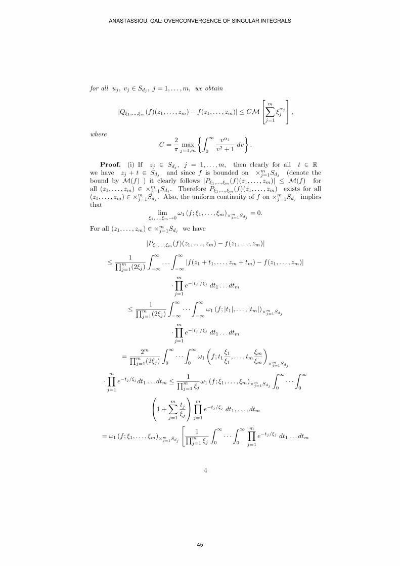
for all uj , vj ∈ Sdj , j = 1, . . . ,m, we obtain
|Qξ1,...,ξm(f)(z1, . . . , zm)− f(z1, . . . , zm)| ≤ CM
m∑
j=1
ξαj
j
,
where
C =2π
maxj=1,m
∫ ∞
0
vαj
v2 + 1dv
.
Proof. (i) If zj ∈ Sdj , j = 1, . . . , m, then clearly for all t ∈ Rwe have zj + t ∈ Sdj and since f is bounded on ×m
j=1Sdj (denote thebound by M(f) ) it clearly follows |Pξ1,...,ξm(f)(z1, . . . , zm)| ≤ M(f) forall (z1, . . . , zm) ∈ ×m
j=1Sdj . Therefore Pξ1,...,ξm(f)(z1, . . . , zm) exists for all(z1, . . . , zm) ∈ ×m
j=1Sdj . Also, the uniform continuity of f on ×mj=1Sdj implies
thatlim
ξ1,...,ξm→0ω1 (f ; ξ1, . . . , ξm)×m
j=1Sdj= 0.
For all (z1, . . . , zm) ∈ ×mj=1Sdj we have
|Pξ1,...,ξm(f)(z1, . . . , zm)− f(z1, . . . , zm)|
≤ 1∏mj=1(2ξj)
∫ ∞
−∞. . .
∫ ∞
−∞|f(z1 + t1, . . . , zm + tm)− f(z1, . . . , zm)|
·m∏
j=1
e−|tj |/ξj dt1 . . . dtm
≤ 1∏mj=1(2ξj)
∫ ∞
−∞· · ·
∫ ∞
−∞ω1 (f ; |t1|, . . . , |tm|)×m
j=1Sdj
·m∏
j=1
e−|tj |/ξj dt1 . . . dtm
=2m
∏mj=1(2ξj)
∫ ∞
0
· · ·∫ ∞
0
ω1
(f ; t1
ξ1
ξ1, . . . , tm
ξm
ξm
)
×mj=1Sdj
·m∏
j=1
e−tj/ξj dt1 . . . dtm ≤ 1∏mj=1 ξj
ω1 (f ; ξ1, . . . , ξm)×mj=1Sdj
∫ ∞
0
· · ·∫ ∞
0
1 +
m∑
j=1
tjξj
m∏
j=1
e−tj/ξj dt1, . . . , dtm
= ω1 (f ; ξ1, . . . , ξm)×mj=1Sdj
[1∏m
j=1 ξj
∫ ∞
0
· · ·∫ ∞
0
m∏
j=1
e−tj/ξj dt1 . . . dtm
4
ANASTASSIOU, GAL: OVERCONVERGENCE OF SINGULAR INTEGRALS
45
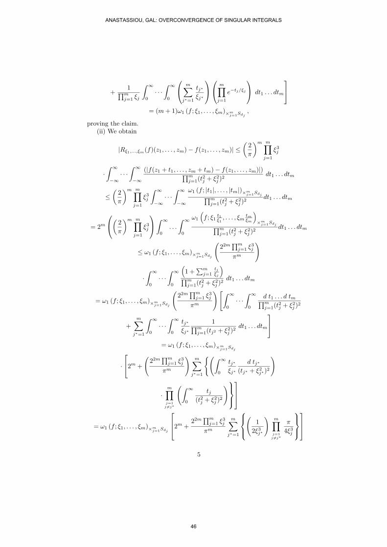
+1∏m
j=1 ξj
∫ ∞
0
· · ·∫ ∞
0
m∑
j∗=1
tj∗
ξj∗
m∏
j=1
e−tj/ξj
dt1 . . . dtm
= (m + 1)ω1 (f ; ξ1, . . . , ξm)×mj=1Sdj
,
proving the claim.(ii) We obtain
|Rξ1,...,ξm(f)(z1, . . . , zm)− f(z1, . . . , zm)| ≤(
2π
)m m∏
j=1
ξ3j
·∫ ∞
−∞· · ·
∫ ∞
−∞
(|f(z1 + t1, . . . , zm + tm)− f(z1, . . . , zm)|)∏mj=1(t
2j + ξ2
j )2dt1 . . . dtm
≤(
2π
)m m∏
j=1
ξ3j
∫ ∞
−∞· · ·
∫ ∞
−∞
ω1 (f ; |t1|, . . . , |tm|)×mj=1Sdj∏m
j=1(t2j + ξ2
j )2dt1 . . . dtm
= 2m
(2π
)m m∏
j=1
ξ3j
∫ ∞
0
. . .
∫ ∞
0
ω1
(f ; ξ1
t1ξ1
, . . . , ξmtm
ξm
)×m
j=1Sdj∏mj=1(t
2j + ξ2
j )2dt1 . . . dtm
≤ ω1 (f ; ξ1, . . . , ξm)×mj=1Sdj
(22m
∏mj=1 ξ3
j
πm
)
·∫ ∞
0
· · ·∫ ∞
0
(1 +
∑mj=1
tj
ξj
)∏m
j=1(t2j + ξ2
j )2dt1 . . . dtm
= ω1 (f ; ξ1, . . . , ξm)×mj=1Sdj
(22m
∏mj=1 ξ3
j
πm
) [∫ ∞
0
· · ·∫ ∞
0
d t1 . . . d tm∏mj=1(t
2j + ξ2
j )2
+m∑
j∗=1
∫ ∞
0
· · ·∫ ∞
0
tj∗
ξj∗
1∏mj=1(tj2 + ξ2
j )2dt1 . . . dtm
= ω1 (f ; ξ1, . . . , ξm)×mj=1Sdj
·2m +
(22m
∏mj=1 ξ3
j
πm
)m∑
j∗=1
(∫ ∞
0
tj∗
ξj∗
d tj∗
(tj∗ + ξ2j∗)2
)
·m∏
j=1j 6=j∗
(∫ ∞
0
tj(t2j + ξ2
j )2
)
= ω1 (f ; ξ1, . . . , ξm)×mj=1Sdj
2m +
22m∏m
j=1 ξ3j
πm
m∑
j∗=1
(1
2ξ3j∗
)m∏
j=1j 6=j∗
π
4ξ3j
5
ANASTASSIOU, GAL: OVERCONVERGENCE OF SINGULAR INTEGRALS
46
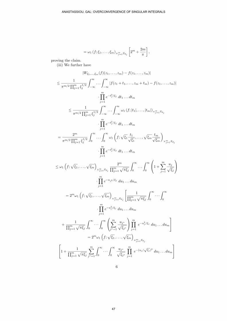
= ω1 (f ; ξ1, . . . , ξm)×mj=1Sdj
[2m +
2m
π
],
proving the claim.(iii) We further have
|Wξ1,...,ξm(f)(z1, . . . , zm)− f(z1, . . . , zm)|
≤ 1
πm/2∏m
j=1 ξ1/2j
∫ ∞
−∞. . .
∫ ∞
−∞|f(z1 + t1, . . . , zm + tm)− f(z1, . . . , zm)|
·m∏
j=1
e−t2j/ξj dt1 . . . dtm
≤ 1
πm/2∏m
j=1 ξ1/2j
∫ ∞
−∞. . .
∫ ∞
−∞ω1 (f ; |t1|, . . . , |tm|)×m
j=1Sdj
·m∏
j=1
e−t2j/ξj dt1 . . . dtm
=2m
πm/2∏m
j=1 ξ1/2j
∫ ∞
0
. . .
∫ ∞
0
ω1
(f ;
√ξ1
t1√ξ1
, . . . ,√
ξmtm√ξm
)
×mj=1Sdj
·m∏
j=1
e−t2j/ξj dt1 . . . dtm
≤ ω1
(f ;
√ξ1, . . . ,
√ξm
)×m
j=1Sdj
2m
∏mj=1
√πξj
∫ ∞
0
. . .
∫ ∞
0
1 +
m∑
j=1
uj√ξj
·m∏
j=1
e−uj2/ξj du1 . . . dum
= 2mω1
(f ;
√ξ1, . . . ,
√ξm
)×m
j=1Sdj
[1∏m
j=1
√πξj
∫ ∞
0
· · ·∫ ∞
0
·m∏
j=1
e−u2j/ξj du1 . . . dum
+1∏m
j=1
√πξj
∫ ∞
0
· · ·∫ ∞
0
m∑
j∗=1
uj∗√ξj∗
m∏
j=1
e−u2j/ξj du1 . . . dum
= 2mω1
(f ;
√ξ1, . . . ,
√ξm
)×m
j=1Sdj1 +
1∏mj=1
√πξj
m∑
j∗=1
∫ ∞
0
· · ·∫ ∞
0
uj∗√ξj∗
m∏
j=1
e−(uj/√
ξj)2
du1 . . . dum
6
ANASTASSIOU, GAL: OVERCONVERGENCE OF SINGULAR INTEGRALS
47
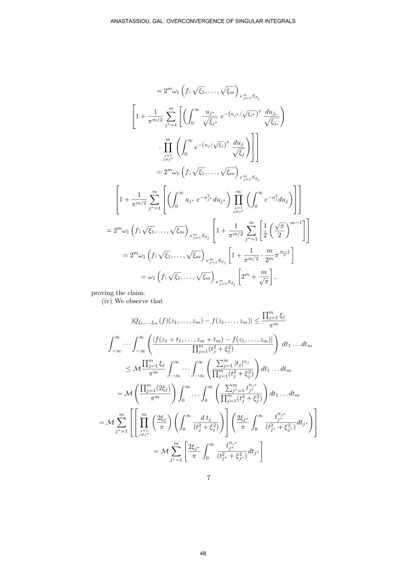
= 2mω1
(f ;
√ξ1, . . . ,
√ξm
)×m
j=1Sdj1 +
1πm/2
m∑
j∗=1
[(∫ ∞
0
uj∗√ξj∗
e−(uj∗/√
ξj∗)2 duj∗√ξj∗
)
·m∏
j=1j 6=j∗
(∫ ∞
0
e−(uj/√
ξj)2 duj√ξj
)
= 2mω1
(f ;
√ξ1, . . . ,
√ξm
)×m
j=1Sdj1 +
1πm/2
m∑
j∗=1
(∫ ∞
0
uj∗ e−u2j∗duj∗
) m∏j=1
j 6=j∗
(∫ ∞
0
e−u2j duj
)
= 2mω1
(f ;
√ξ1, . . . ,
√ξm
)×m
j=1Sdj
1 +
1πm/2
m∑
j∗=1
[12
(√π
2
)m−1]
= 2mω1
(f ;
√ξ1, . . . ,
√ξm
)×m
j=1Sdj
[1 +
1πm/2
· m
2mπ
m−12
]
= ω1
(f ;
√ξ1, . . . ,
√ξm
)×m
j=1Sdj
[2m +
m√π
],
proving the claim.(iv) We observe that
|Qξ1,...,ξm(f)(z1, . . . , zm)− f(z1, . . . , zm)| ≤∏m
j=1 ξj
πm
·∫ ∞
−∞· · ·
∫ ∞
−∞
(|f(z1 + t1, . . . , zm + tm)− f(z1, . . . , zm)|∏m
j=1(t2j + ξ2
j )
)dt1 . . . dtm
≤M∏m
j=1 ξj
πm
∫ ∞
−∞· · ·
∫ ∞
−∞
( ∑mj=1 |tj |αj
∏mj=1(t
2j + ξ2
j )
)dt1 . . . dtm
= M(∏m
j=1(2ξj)πm
) ∫ ∞
0
. . .
∫ ∞
0
( ∑mj∗=1 t
αj∗j∗∏m
j=1(t2j + ξ2
j )
)dt1 . . . dtm
= Mm∑
j∗=1
m∏j=1
j 6=j∗
(2ξj
π
) (∫ ∞
0
d tj(t2j + ξ2
j )
)
(2ξj∗
π
∫ ∞
0
tαj∗j∗
(t2j∗ + ξ2j∗)
dtj∗
)
= Mm∑
j∗=1
[2ξj∗
π
∫ ∞
0
tαj∗j∗
(t2j∗ + ξ2j∗)
dtj∗
]
7
ANASTASSIOU, GAL: OVERCONVERGENCE OF SINGULAR INTEGRALS
48
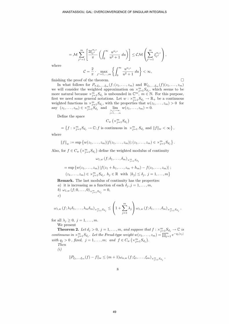
= Mm∑
j∗=1
[2ξ
αj∗j∗
π
(∫ ∞
0
uαj∗
u2 + 1du
)]≤ CM
m∑
j∗=1
ξαj∗j∗
,
where
C =2π· max
j∗=1,...,m
∫ ∞
0
uαj∗
u2 + 1du
< ∞,
finishing the proof of the theorem. ¤In what follows for Pn,ξ1,...,ξm(f ; (z1, . . . , zm) and Wξ1,...,ξm(f)(z1, . . . , zm)
we will consider the weighted approximation on ×mj=1Sdj , which seems to be
more natural because ×mj=1Sdj is unbounded in Cm, m ∈ N. For this purpose,
first we need some general notations. Let w : ×mj=1Sdj → R+ be a continuous
weighted functions in ×mj=1Sdj , with the properties that w(z1, . . . , zm) > 0 for
any (z1, . . . , zm) ∈ ×mj=1Sdj and lim
|zj |→∞,
j=1,...,m
w(z1, . . . , zm) = 0.
Define the spaceCw
(×mj=1Sdj
)
=f : ×m
j=1Sdj → C; f is continuous in ×mj=1 Sdj and ‖f‖w < ∞
,
where
‖f‖w := supw(z1, . . . , zm)|f(z1, . . . , zm)|; (z1, . . . , zm) ∈ ×m
j=1Sdj
.
Also, for f ∈ Cw
(×mj=1Sdj
)define the weighted modulus of continuity
ω1,w (f ; δ1, . . . , δm)×mj=1Sdj
= sup w(z1, . . . , zm) |f(z1 + h1, . . . , zm + hm)− f(z1, . . . , zm)| ;(z1, . . . , zm) ∈ ×m
j=1Sdj , hj ∈ R with |hj | ≤ δj , j = 1, . . . , m
Remark. The last modulus of continuity has the properties:a) it is increasing as a function of each δj , j = 1, . . . , m,b) ω1,w (f ; 0, . . . , 0)×m
j=1Sdj= 0,
c)
ω1,w (f ;λ1δ1, . . . , λmδm)×mj=1Sdj
≤1 +
m∑
j=1
λj
ω1,w (f ; δ1, . . . , δm)×m
j=1Sdj,
for all λj ≥ 0, j = 1, . . . , m.We presentTheorem 2. Let dj > 0, j = 1, . . . , m, and suppose that f : ×m
j=1Sdj → C iscontinuous in ×m
j=1Sdj. Let the Freud-type weight w(z1, . . . , zm) =
∏mj=1 e−qj |zj |
with qj > 0 , fixed, j = 1, . . . , m; and f ∈ Cw
(×mj=1Sdj
).
Then(i)
‖Pξ1,...,ξm(f)− f‖w ≤ (m + 1)ωn,w (f ; ξ1, . . . , ξm)×mj=1Sdj
,
8
ANASTASSIOU, GAL: OVERCONVERGENCE OF SINGULAR INTEGRALS
49

for all 0 < ξj < 1qj
, j = 1, . . . , m, and(ii)
‖W ∗ξ (f)− f‖w ≤
(2m +
m√π
)ω1,w
(f ;
√ξ1, . . . ,
√ξm
)×m
j=1Sdj
,
for all 0 < ξj < 1, j = 1, . . . , m.Proof. The continuity of f in ×m
j=1Sdj immediately implies the continuityof Pξ1,...,ξm(f) and Wξ1,...,ξm(f)(z1, . . . , zm).
(i) In addition we have
|w(z1, . . . , zm)Pξ1,...,ξm(f)(z1, . . . , zm)|
=
∣∣∣∣∣1∏m
j=1(2ξj)
∫ ∞
−∞· · ·
∫ ∞
−∞w(z1 + t1, . . . , zm + tm)f(z1 + t1, . . . , tm)
· w(z1, . . . , zm)w(z1 + t1, . . . , zm + tm)
m∏
j=1
e−|tj |/ξj dt1 . . . dtm
∣∣∣∣∣∣
≤ ‖f‖w
m∏
j=1
12ξj
∫ ∞
−∞e|tj |
(qj− 1
ξj
)dtj ≤
m∏
j=1
Cξj ,qj
‖f‖w ,
whereCξj ,qj =
12ξj
∫ ∞
−∞e|tj |
(qj− 1
ξj
)dtj < ∞,
for all j = 1, . . . ,m.Passing to supremum over all (z1, . . . , zm) ∈ ×m
j=1Sdj , it follows that‖Pξ1,...,ξm(f)‖w < ∞, that is Pξ1,...,ξm(f) ∈ Cw
(×mj=1Sdj
), for 0 < ξj < 1
qj, j =
1, . . . , m.Next for all zj ∈ Sdj , j = 1, . . . , m, we derive
w(z1, . . . , zm)|Pξ1,...,ξm(f)(z1, . . . , zm)− f(z1, . . . , zm)|
=w(z1, . . . , zm)∏m
j=1(2ξj)
∣∣∣∣∫ ∞
−∞· · ·
∫ ∞
−∞(f(z1 + t1, . . . , zm + tm)− f(z1, . . . , zm))
·m∏
j=1
e−|tj |/ξj dt1 . . . dtm
∣∣∣∣∣∣≤ 1∏m
j=1(2ξj)
·∫ ∞
−∞· · ·
∫ ∞
−∞w(z1, . . . , zm) |f(z1 + t1, . . . , zm + tm)− f(z1, . . . , zm)|
·m∏
j=1
e−|tj |/ξj dt1 . . . dtm
9
ANASTASSIOU, GAL: OVERCONVERGENCE OF SINGULAR INTEGRALS
50
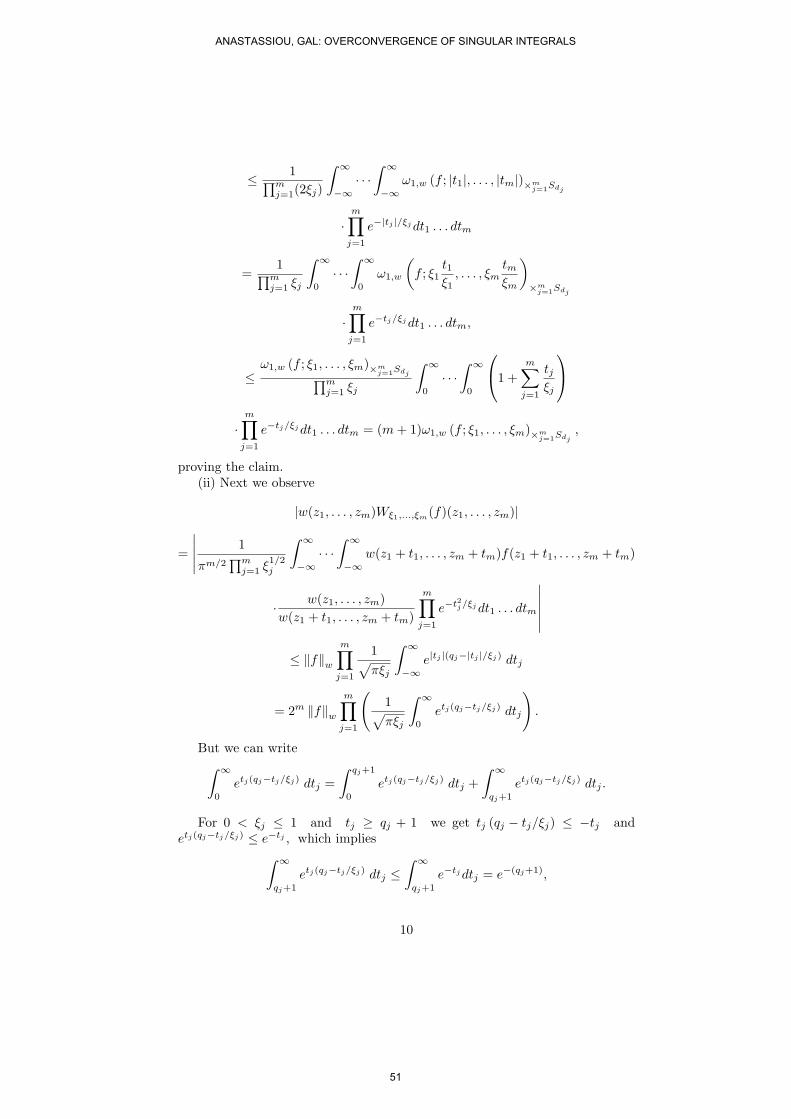
≤ 1∏mj=1(2ξj)
∫ ∞
−∞· · ·
∫ ∞
−∞ω1,w (f ; |t1|, . . . , |tm|)×m
j=1Sdj
·m∏
j=1
e−|tj |/ξj dt1 . . . dtm
=1∏m
j=1 ξj
∫ ∞
0
· · ·∫ ∞
0
ω1,w
(f ; ξ1
t1ξ1
, . . . , ξmtmξm
)
×mj=1Sdj
·m∏
j=1
e−tj/ξj dt1 . . . dtm,
≤ω1,w (f ; ξ1, . . . , ξm)×m
j=1Sdj∏mj=1 ξj
∫ ∞
0
· · ·∫ ∞
0
1 +
m∑
j=1
tjξj
·m∏
j=1
e−tj/ξj dt1 . . . dtm = (m + 1)ω1,w (f ; ξ1, . . . , ξm)×mj=1Sdj
,
proving the claim.(ii) Next we observe
|w(z1, . . . , zm)Wξ1,...,ξm(f)(z1, . . . , zm)|
=
∣∣∣∣∣1
πm/2∏m
j=1 ξ1/2j
∫ ∞
−∞· · ·
∫ ∞
−∞w(z1 + t1, . . . , zm + tm)f(z1 + t1, . . . , zm + tm)
· w(z1, . . . , zm)w(z1 + t1, . . . , zm + tm)
m∏
j=1
e−t2j/ξj dt1 . . . dtm
∣∣∣∣∣∣
≤ ‖f‖w
m∏
j=1
1√πξj
∫ ∞
−∞e|tj |(qj−|tj |/ξj) dtj
= 2m ‖f‖w
m∏
j=1
(1√πξj
∫ ∞
0
etj(qj−tj/ξj) dtj
).
But we can write∫ ∞
0
etj(qj−tj/ξj) dtj =∫ qj+1
0
etj(qj−tj/ξj) dtj +∫ ∞
qj+1
etj(qj−tj/ξj) dtj .
For 0 < ξj ≤ 1 and tj ≥ qj + 1 we get tj (qj − tj/ξj) ≤ −tj andetj(qj−tj/ξj) ≤ e−tj , which implies
∫ ∞
qj+1
etj(qj−tj/ξj) dtj ≤∫ ∞
qj+1
e−tj dtj = e−(qj+1),
10
ANASTASSIOU, GAL: OVERCONVERGENCE OF SINGULAR INTEGRALS
51
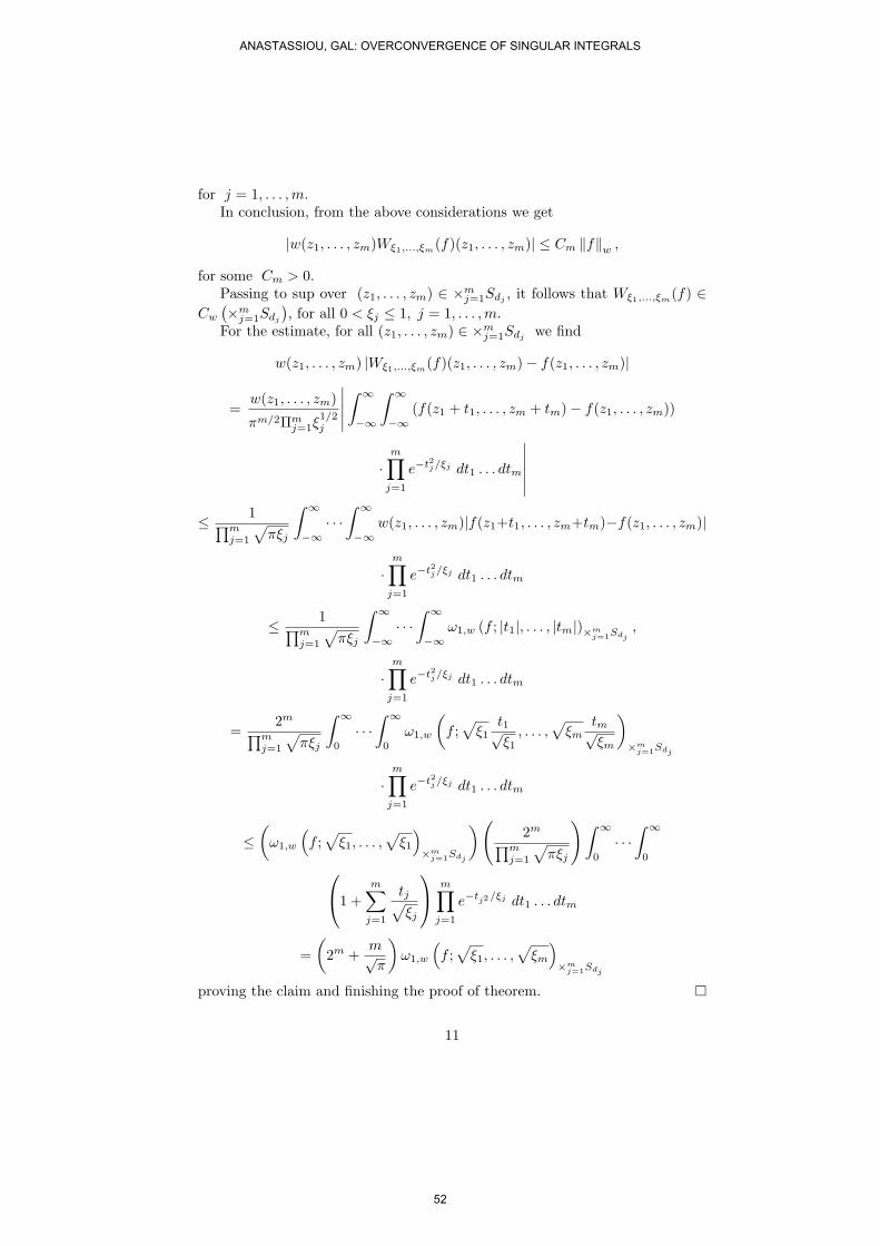
for j = 1, . . . , m.In conclusion, from the above considerations we get
|w(z1, . . . , zm)Wξ1,...,ξm(f)(z1, . . . , zm)| ≤ Cm ‖f‖w ,
for some Cm > 0.Passing to sup over (z1, . . . , zm) ∈ ×m
j=1Sdj , it follows that Wξ1,...,ξm(f) ∈Cw
(×mj=1Sdj
), for all 0 < ξj ≤ 1, j = 1, . . . , m.
For the estimate, for all (z1, . . . , zm) ∈ ×mj=1Sdj we find
w(z1, . . . , zm) |Wξ1,...,ξm(f)(z1, . . . , zm)− f(z1, . . . , zm)|
=w(z1, . . . , zm)
πm/2Πmj=1ξ
1/2j
∣∣∣∣∣∫ ∞
−∞
∫ ∞
−∞(f(z1 + t1, . . . , zm + tm)− f(z1, . . . , zm))
·m∏
j=1
e−t2j/ξj dt1 . . . dtm
∣∣∣∣∣∣
≤ 1∏mj=1
√πξj
∫ ∞
−∞· · ·
∫ ∞
−∞w(z1, . . . , zm)|f(z1+t1, . . . , zm+tm)−f(z1, . . . , zm)|
·m∏
j=1
e−t2j/ξj dt1 . . . dtm
≤ 1∏mj=1
√πξj
∫ ∞
−∞· · ·
∫ ∞
−∞ω1,w (f ; |t1|, . . . , |tm|)×m
j=1Sdj,
·m∏
j=1
e−t2j/ξj dt1 . . . dtm
=2m
∏mj=1
√πξj
∫ ∞
0
· · ·∫ ∞
0
ω1,w
(f ;
√ξ1
t1√ξ1
, . . . ,√
ξmtm√ξm
)
×mj=1Sdj
·m∏
j=1
e−t2j/ξj dt1 . . . dtm
≤(
ω1,w
(f ;
√ξ1, . . . ,
√ξ1
)×m
j=1Sdj
) (2m
∏mj=1
√πξj
) ∫ ∞
0
· · ·∫ ∞
0
1 +
m∑
j=1
tj√ξj
m∏
j=1
e−tj2/ξj dt1 . . . dtm
=(
2m +m√π
)ω1,w
(f ;
√ξ1, . . . ,
√ξm
)×m
j=1Sdj
proving the claim and finishing the proof of theorem. ¤
11
ANASTASSIOU, GAL: OVERCONVERGENCE OF SINGULAR INTEGRALS
52
References
[1] G. A. Anastassiou and S. G. Gal, Convergence of generalized singular in-tegrals to the unit, multivariate case, in : Applied Mathematics Reviews(G. A. Anastassiou ed.) , vol. 1, World Scientific, Singapore, New Jersey,London, Hong Kong, 2000, pp. 1-8.
[2] G. A. Anastassiou and S. G. Gal, Quantitative estimates in the overcon-vergence of some singular integrals, Communications in Applied Analysis,under press.
12
ANASTASSIOU, GAL: OVERCONVERGENCE OF SINGULAR INTEGRALS
53

A note on strong di¤erential superordinations using S¼al¼agean andRuscheweyh operators
Alina Alb LupasDepartment of Mathematics and Computer Science
University of Oradeastr. Universitatii nr. 1, 410087 Oradea, Romania
Abstract
In the present paper we establish several strong di¤erential superordinations regardind the new operatorSRm dened by convolution product of the extended S¼al¼agean operator and Ruscheweyh derivative, SRm :
An ! A
n ; SRmf (z; ) = (Sm Rm) f (z; ) ; z 2 U; 2 U; where Rmf(z; ) denote the extended
Ruscheweyh derivative, Smf(z; ) is the extended S¼al¼agean operator and An = ff 2 H(U U); f(z; ) =
z + an+1 () zn+1 + : : : ; z 2 U; 2 Ug is the class of normalized analytic functions.
Keywords: strong di¤erential superordination, convex function, best subordinant, extended di¤erential oper-ator, convolution product.2000 Mathematical Subject Classication: 30C45, 30A20, 34A40.
1 Introduction
Denote by U the unit disc of the complex plane U = fz 2 C : jzj < 1g, U = fz 2 C : jzj 1g the closedunit disc of the complex plane and H(U U) the class of analytic functions in U U .Let An = ff 2 H(U U); f(z; ) = z + an+1 () zn+1 + : : : ; z 2 U; 2 Ug; where ak () are holomorphic
functions in U for k 2; and H[a; n; ] = ff 2 H(U U); f(z; ) = a+ an () zn+ an+1 () zn+1+ : : : ; z 2 U; 2 Ug; for a 2 C, n 2 N; ak () are holomorphic functions in U for k n:We also extend the well known di¤erential operators to the new class of analytic functions An introduced
in [5].
Denition 1.1 [1] For f 2 An , n;m 2 N; the operator Sm is dened by Sm : An ! An ,
S0f (z; ) = f (z; ) ;
S1f (z; ) = zf 0z(z; ); :::;
Sm+1f(z; ) = z (Smf (z; ))0z , z 2 U; 2 U:
Remark 1.2 [1] If f 2 An , f(z; ) = z +P1
j=n+1 aj () zj, then Smf (z; ) = z +
P1j=n+1 j
maj () zj, z 2 U;
2 U .
Denition 1.3 [1] For f 2 An , n;m 2 N; the operator Rm is dened by Rm : An ! An ,
R0f (z; ) = f (z; ) ;
R1f (z; ) = zf 0z (z; ) ; :::;
(m+ 1)Rm+1f (z; ) = z (Rmf (z; ))0z +mR
mf (z; ) , z 2 U; 2 U:
1
54
JOURNAL OF APPLIED FUNCTIONAL ANALYSIS, VOL.7, NO’S 1-2,54-61,COPYRIGHT 2012 EUDOXUS PRESS,LLC

Remark 1.4 [1] If f 2 An , f(z; ) = z +P1
j=n+1 aj () zj, then Rmf (z; ) = z +
P1j=n+1 C
mm+j1aj () z
j,z 2 U; 2 U:
As a dual notion of strong di¤erential subordination G.I. Oros has introduced and developed the notion ofstrong di¤erential superordinations in [4].
Denition 1.5 [4] Let f (z; ), H (z; ) analytic in U U: The function f (z; ) is said to be strongly su-perordinate to H (z; ) if there exists a function w analytic in U , with w (0) = 0 and jw (z)j < 1; such thatH (z; ) = f (w (z) ; ) ; for all 2 U . In such a case we write H (z; ) f (z; ) ; z 2 U; 2 U:
Remark 1.6 [4] (i) Since f (z; ) is analytic in U U , for all 2 U; and univalent in U; for all 2 U ,Denition 1.5 is equivalent to H (0; ) = f (0; ) ; for all 2 U; and H
U U
f
U U
:
(ii) If H (z; ) H (z) and f (z; ) f (z) ; the strong superordination becomes the usual notion of superor-dination.
Denition 1.7 [3] We denote by Q the set of functions that are analytic and injective on U UnE (f; ),where E (f; ) = fy 2 @U : lim
z!yf (z; ) = 1g; and are such that f 0z (y; ) 6= 0 for y 2 @U UnE (f; ). The
subclass of Q for which f (0; ) = a is denoted by Q (a).
We have need the following lemmas to study the strong di¤erential superordinations.
Lemma 1.8 [3] Let h (z; ) be a convex function with h(0; ) = a and let 2 C be a complex number withRe 0. If p 2 H[a; n; ]\Q; p(z; )+ 1
zp0z(z; ) is univalent in U U and h(z; ) p(z; )+ 1
zp0z(z; );
z 2 U; 2 U;then q(z; ) p(z; ); z 2 U; 2 U; where q(z; ) =
nz n
R z0h (t; ) t
n1dt; z 2 U; 2 U: The
function q is convex and is the best subordinant.
Lemma 1.9 [3] Let q (z; ) be a convex function in U U and let h(z; ) = q(z; ) + 1 zq
0z(z; ); z 2 U; 2 U;
where Re 0. If p 2 H [a; n; ] \Q, p(z; ) + 1 zp
0z(z; ) is univalent in U U and q(z; ) + 1
zq0z(z; )
p(z; )+ 1 zp
0z (z; ) ; z 2 U; 2 U; then q(z; ) p(z; ); z 2 U; 2 U; where q(z; ) =
nz n
R z0h (t; ) t
n1dt;
z 2 U , 2 U: The function q is the best subordinant.
2 Main results
Denition 2.1 [2] Let m 2 N [ f0g. Denote by SRm the operator given by the Hadamard product (theconvolution product) of the extended S¼al¼agean operator Sm and the extended Ruscheweyh operator Rm, SRm :An ! An ,
SRmf (z; ) = (Sm Rm) f (z; ) :
Remark 2.2 [2] If f 2 An , f(z; ) = z+P1
j=n+1 aj () zj ; then SRmf (z; ) = z+
P1j=n+1 C
mm+j1j
ma2j () zj ;
z 2 U; 2 U:
Theorem 2.3 Let h (z; ) be a convex function in U U with h (0; ) = 1. Let m 2 N, f (z; ) 2 An ;F (z; ) = Ic (f) (z; ) =
c+2zc+1
R z0tcf (t; ) dt, z 2 U; 2 U , Re c > 2; and suppose that (SRmf (z; ))0z is
univalent in U U , (SRmF (z; ))0z 2 H [1; n; ] \Q and
h (z; ) (SRmf (z; ))0z , z 2 U; 2 U; (1)
thenq (z; ) (SRmF (z; ))0z , z 2 U; 2 U;
where q(z; ) = c+2
nzc+2n
R z0h(t; )t
c+2n 1dt: The function q is convex and it is the best subordinant.
2
LUPAS: STRONG DIFFERENTIAL SUPERORDINATIONS...
55

Proof. We have zc+1F (z; ) = (c+ 2)R z0tcf (t; ) dt and di¤erentiating it, with respect to z, we obtain
(c+ 1)F (z; )+ zF 0z (z; ) = (c+ 2) f (z; ) and (c+ 1)SRmF (z; )+ z (SRmF (z; ))
0z = (c+ 2)SR
mf (z; ) ;
z 2 U; 2 U:Di¤erentiating the last relation with respect to z we have
(SRmF (z; ))0z +
1
c+ 2z (SRmF (z; ))
00z2 = (SR
mf (z; ))0z , z 2 U; 2 U: (2)
Using (2), the strong di¤erential superordination (1) becomes
h (z; ) (SRmF (z; ))0z +1
c+ 2z (SRmF (z; ))
00z2 : (3)
Denotep (z; ) = (SRmF (z; ))
0z ; z 2 U; 2 U: (4)
Replacing (4) in (3) we obtain h (z; ) p (z; ) + 1c+2zp
0z (z; ), z 2 U; 2 U:
Using Lemma 1.8 for = c+ 2; we have
q (z; ) p (z; ) ; z 2 U; 2 U; i.e. q (z; ) (SRmF (z; ))0z , z 2 U; 2 U;
where q(z; ) = c+2
nzc+2n
R z0h(t; )t
c+2n 1dt: The function q is convex and it is the best subordinant.
Corollary 2.4 Let h (z; ) = +(2)z1+z ; where 2 [0; 1). Let m 2 N, f (z; ) 2 An ; F (z; ) = Ic (f) (z; ) =
c+2zc+1
R z0tcf (t; ) dt, z 2 U; 2 U; Re c > 2; and suppose that (SRmf (z; ))0z is univalent in U U ,
(SRmF (z; ))0z 2 H [1; n; ] \Q and
h (z; ) (SRmf (z; ))0z , z 2 U; 2 U; (5)
thenq (z; ) (SRmF (z; ))0z , z 2 U; 2 U;
where q is given by q(z; ) = 2 + 2(c+2)()nz
c+2n
R z0tc+2n
1
t+1 dt; z 2 U; 2 U: The function q is convex and it isthe best subordinant.
Proof. Following the same steps as in the proof of Theorem 2.3 and considering p(z; ) = (SRmF (z; ))0z,the strong di¤erential superordination (5) becomes h(z; ) = +(2)z
1+z p (z; ) + 1c+2zp
0z (z; ) ; z 2 U;
2 U:By using Lemma 1.8 for = c + 2, we have q(z; ) p(z; ), i.e. q(z; ) = c+2
nzc+2n
R z0h(t; )t
c+2n 1dt =
c+2
nzc+2n
R z0+(2)t
1+t tc+2n 1dt = 2 + 2(c+2)()
nzc+2n
R z0tc+2n
1
t+1 dt (SRmF (z; ))0z ; z 2 U; 2 U:The function q is convex and it is the best subordinant.
Theorem 2.5 Let q (z; ) be a convex function in U U and let h (z; ) = q (z; )+ 1c+2zq
0z (z; ) ; where z 2 U;
2 U; Re c > 2: Let m 2 N, f (z; ) 2 An ; F (z; ) = Ic (f) (z; ) = c+2zc+1
R z0tcf (t; ) dt, z 2 U; 2 U; and
suppose that (SRmf (z; ))0z is univalent in U U , (SRmF (z; ))0z 2 H [1; n; ] \Q and
h (z; ) (SRmf (z; ))0z , z 2 U; 2 U; (6)
thenq (z; ) (SRmF (z; ))0z , z 2 U; 2 U;
where q(z; ) = c+2
nzc+2n
R z0h(t; )t
c+2n 1dt: The function q is the best subordinant.
3
LUPAS: STRONG DIFFERENTIAL SUPERORDINATIONS...
56

Proof. We obtain that
zc+1F (z; ) = (c+ 2)
Z z
0
tcf (t; ) dt: (7)
Di¤erentiating (7), with respect to z, we have (c+ 1)F (z; ) + zF 0z (z; ) = (c+ 2) f (z; ) and
(c+ 1)SRmF (z; ) + z (SRmF (z; ))0z = (c+ 2)SR
mf (z; ) ; z 2 U; 2 U: (8)
Di¤erentiating (8) with respect to z we have
(SRmF (z; ))0z +
1
c+ 2z (SRmF (z; ))
00z2 = (SR
mf (z; ))0z , z 2 U; 2 U: (9)
Using (9), the strong di¤erential superordination (6) becomes
h (z; ) = q (z; ) +1
c+ 2zq0z (z; ) (SRmF (z; ))
0z +
1
c+ 2z (SRmF (z; ))
00z2 : (10)
Denotep (z; ) = (SRmF (z; ))
0z ; z 2 U; 2 U: (11)
Replacing (11) in (10) we obtain h (z; ) = q (z; ) + 1c+2zq
0z (z; ) p (z; ) + 1
c+2zp0z (z; ), z 2 U; 2 U:
Using Lemma 1.9 for = c+ 2; we have
q (z; ) p (z; ) ; z 2 U; 2 U; i.e. q (z; ) (SRmF (z; ))0z , z 2 U; 2 U;
where q(z; ) = c+2
nzc+2n
R z0h(t; )t
c+2n 1dt: The function q is the best subordinant.
Theorem 2.6 Let h (z; ) be a convex function, h(0; ) = 1: Let m 2 N; f (z; ) 2 An and suppose that(SRmf (z; ))
0z is univalent and
SRmf(z;)z 2 H [1; n; ] \Q. If
h(z; ) (SRmf (z; ))0z ; z 2 U; 2 U; (12)
then
q(z; ) SRmf (z; )
z; z 2 U; 2 U;
where q(z; ) = 1
nz1n
R z0h(t; )t
1n1dt: The function q is convex and it is the best subordinant.
Proof. Consider p (z; ) = SRmf(z;)z =
z+P1
j=n+1Cmm+j1j
ma2j ()zj
z = 1 +P1
j=n+1 Cmm+j1j
ma2j () zj1:
Evidently p 2 H[1; n; ].Di¤erentiating with respect to z, we obtain p (z; ) + zp0z (z; ) = (SR
mf (z; ))0z :
Then (12) becomes h(z; ) p(z; ) + zp0z(z; ); z 2 U; 2 U:By using Lemma 1.8 for = 1, we have
q(z; ) p(z; ); z 2 U; 2 U; i.e. q(z; ) SRmf (z; )
z; z 2 U; 2 U;
where q(z; ) = 1
nz1n
R z0h(t; )t
1n1dt: The function q is convex and it is the best subordinant.
Corollary 2.7 Let h(z; ) = +(2)z1+z be a convex function in U U , where 0 < 1. Let m 2 N [ f0g;
f (z; ) 2 An and suppose that (SRmf (z; ))0z is univalent and
SRmf(z;)z 2 H [1; n; ] \Q. If
h(z; ) (SRmf (z; ))0z ; z 2 U; 2 U; (13)
then
q(z; ) SRmf (z; )
z; z 2 U; 2 U;
where q is given by q(z; ) = 2 + 2()nz
1n
R z0t1n1
1+t dt; z 2 U; 2 U: The function q is convex and it is thebest subordinant.
4
LUPAS: STRONG DIFFERENTIAL SUPERORDINATIONS...
57
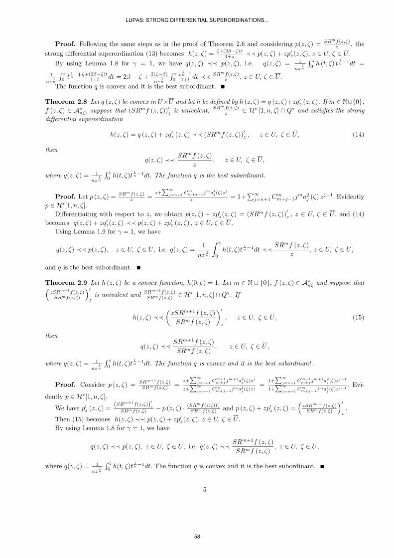
Proof. Following the same steps as in the proof of Theorem 2.6 and considering p(z; ) = SRmf(z;)z , the
strong di¤erential superordination (13) becomes h(z; ) = +(2)z1+z p(z; ) + zp0z(z; ); z 2 U; 2 U:
By using Lemma 1.8 for = 1, we have q(z; ) p(z; ), i.e. q(z; ) = 1
nz1n
R z0h (t; ) t
1n1dt =
1
nz1n
R z0t1n1 +(2)t
1+t dt = 2 + 2()nz
1n
R z0t1n1
1+t dt SRmf(z;)
z ; z 2 U; 2 U:The function q is convex and it is the best subordinant.
Theorem 2.8 Let q (z; ) be convex in UU and let h be dened by h (z; ) = q (z; )+zq0z (z; ) : If m 2 N[f0g,f (z; ) 2 An , suppose that (SRmf (z; ))
0z is univalent,
SRmf(z;)z 2 H [1; n; ] \ Q and satises the strong
di¤erential superordination
h(z; ) = q (z; ) + zq0z (z; ) (SRmf (z; ))0z ; z 2 U; 2 U; (14)
then
q(z; ) SRmf (z; )
z; z 2 U; 2 U;
where q(z; ) = 1
nz1n
R z0h(t; )t
1n1dt: The function q is the best subordinant.
Proof. Let p (z; ) = SRmf(z;)z =
z+P1
j=n+1Cmm+j1j
ma2j ()zj
z = 1+P1
j=n+1 Cmm+j1j
ma2j () zj1: Evidently
p 2 H[1; n; ].Di¤erentiating with respect to z, we obtain p(z; ) + zp0z(z; ) = (SRmf (z; ))
0z ; z 2 U; 2 U; and (14)
becomes q(z; ) + zq0z(z; ) p(z; ) + zp0z (z; ) ; z 2 U; 2 U:Using Lemma 1.9 for = 1, we have
q(z; ) p(z; ); z 2 U; 2 U; i.e. q(z; ) = 1
nz1n
Z z
0
h(t; )t1n1dt SRmf (z; )
z, z 2 U; 2 U;
and q is the best subordinant.
Theorem 2.9 Let h (z; ) be a convex function, h(0; ) = 1: Let m 2 N [ f0g; f (z; ) 2 An and suppose thatzSRm+1f(z;)SRmf(z;)
0zis univalent and SRm+1f(z;)
SRmf(z;) 2 H [1; n; ] \Q. If
h(z; ) zSRm+1f (z; )
SRmf (z; )
0z
; z 2 U; 2 U; (15)
then
q(z; ) SRm+1f (z; )
SRmf (z; ); z 2 U; 2 U;
where q(z; ) = 1
nz1n
R z0h(t; )t
1n1dt: The function q is convex and it is the best subordinant.
Proof. Consider p (z; ) = SRm+1f(z;)SRmf(z;) =
z+P1
j=n+1Cm+1m+j j
m+1a2j ()zj
z+P1
j=n+1Cmm+j1j
ma2j ()zj=
1+P1
j=n+1Cm+1m+j j
m+1a2j ()zj1
1+P1
j=n+1Cmm+j1j
ma2j ()zj1: Evi-
dently p 2 H[1; n; ].
We have p0z (z; ) =(SRm+1f(z;))
0z
SRmf(z;) p (z; ) (SRmf(z;))0z
SRmf(z;) and p (z; ) + zp0z (z; ) =zSRm+1f(z;)SRmf(z;)
0z:
Then (15) becomes h(z; ) p(z; ) + zp0z(z; ); z 2 U; 2 U:By using Lemma 1.8 for = 1, we have
q(z; ) p(z; ); z 2 U; 2 U; i.e. q(z; ) SRm+1f (z; )
SRmf (z; ); z 2 U; 2 U;
where q(z; ) = 1
nz1n
R z0h(t; )t
1n1dt: The function q is convex and it is the best subordinant.
5
LUPAS: STRONG DIFFERENTIAL SUPERORDINATIONS...
58
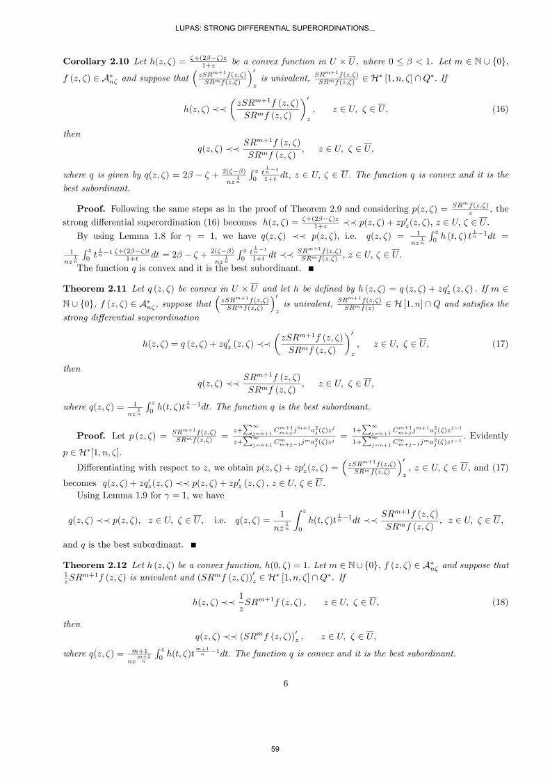
Corollary 2.10 Let h(z; ) = +(2)z1+z be a convex function in U U , where 0 < 1. Let m 2 N [ f0g;
f (z; ) 2 An and suppose thatzSRm+1f(z;)SRmf(z;)
0zis univalent, SR
m+1f(z;)SRmf(z;) 2 H [1; n; ] \Q: If
h(z; ) zSRm+1f (z; )
SRmf (z; )
0z
; z 2 U; 2 U; (16)
then
q(z; ) SRm+1f (z; )
SRmf (z; ); z 2 U; 2 U;
where q is given by q(z; ) = 2 + 2()nz
1n
R z0t1n1
1+t dt; z 2 U; 2 U: The function q is convex and it is thebest subordinant.
Proof. Following the same steps as in the proof of Theorem 2.9 and considering p(z; ) = SRmf(z;)z , the
strong di¤erential superordination (16) becomes h(z; ) = +(2)z1+z p(z; ) + zp0z(z; ); z 2 U; 2 U:
By using Lemma 1.8 for = 1, we have q(z; ) p(z; ), i.e. q(z; ) = 1
nz1n
R z0h (t; ) t
1n1dt =
1
nz1n
R z0t1n1 +(2)t
1+t dt = 2 + 2()nz
1n
R z0t1n1
1+t dt SRm+1f(z;)SRmf(z;) ; z 2 U; 2 U:
The function q is convex and it is the best subordinant.
Theorem 2.11 Let q (z; ) be convex in U U and let h be dened by h (z; ) = q (z; ) + zq0z (z; ) : If m 2N [ f0g, f (z; ) 2 An , suppose that
zSRm+1f(z;)SRmf(z;)
0zis univalent, SR
m+1f(z;)SRmf(z) 2 H [1; n] \Q and satises the
strong di¤erential superordination
h(z; ) = q (z; ) + zq0z (z; ) zSRm+1f (z; )
SRmf (z; )
0z
; z 2 U; 2 U; (17)
then
q(z; ) SRm+1f (z; )
SRmf (z; ); z 2 U; 2 U;
where q(z; ) = 1
nz1n
R z0h(t; )t
1n1dt: The function q is the best subordinant.
Proof. Let p (z; ) = SRm+1f(z;)SRmf(z;) =
z+P1
j=n+1Cm+1m+j j
m+1a2j ()zj
z+P1
j=n+1Cmm+j1j
ma2j ()zj=
1+P1
j=n+1Cm+1m+j j
m+1a2j ()zj1
1+P1
j=n+1Cmm+j1j
ma2j ()zj1: Evidently
p 2 H[1; n; ].
Di¤erentiating with respect to z, we obtain p(z; ) + zp0z(z; ) =zSRm+1f(z;)SRmf(z;)
0z; z 2 U; 2 U; and (17)
becomes q(z; ) + zq0z(z; ) p(z; ) + zp0z (z; ) ; z 2 U; 2 U:Using Lemma 1.9 for = 1, we have
q(z; ) p(z; ); z 2 U; 2 U; i.e. q(z; ) =1
nz1n
Z z
0
h(t; )t1n1dt SRm+1f (z; )
SRmf (z; ), z 2 U; 2 U;
and q is the best subordinant.
Theorem 2.12 Let h (z; ) be a convex function, h(0; ) = 1: Let m 2 N[f0g; f (z; ) 2 An and suppose that1zSR
m+1f (z; ) is univalent and (SRmf (z; ))0z 2 H [1; n; ] \Q. If
h(z; ) 1
zSRm+1f (z; ) ; z 2 U; 2 U; (18)
thenq(z; ) (SRmf (z; ))0z ; z 2 U; 2 U;
where q(z; ) = m+1
nzm+1n
R z0h(t; )t
m+1n 1dt: The function q is convex and it is the best subordinant.
6
LUPAS: STRONG DIFFERENTIAL SUPERORDINATIONS...
59
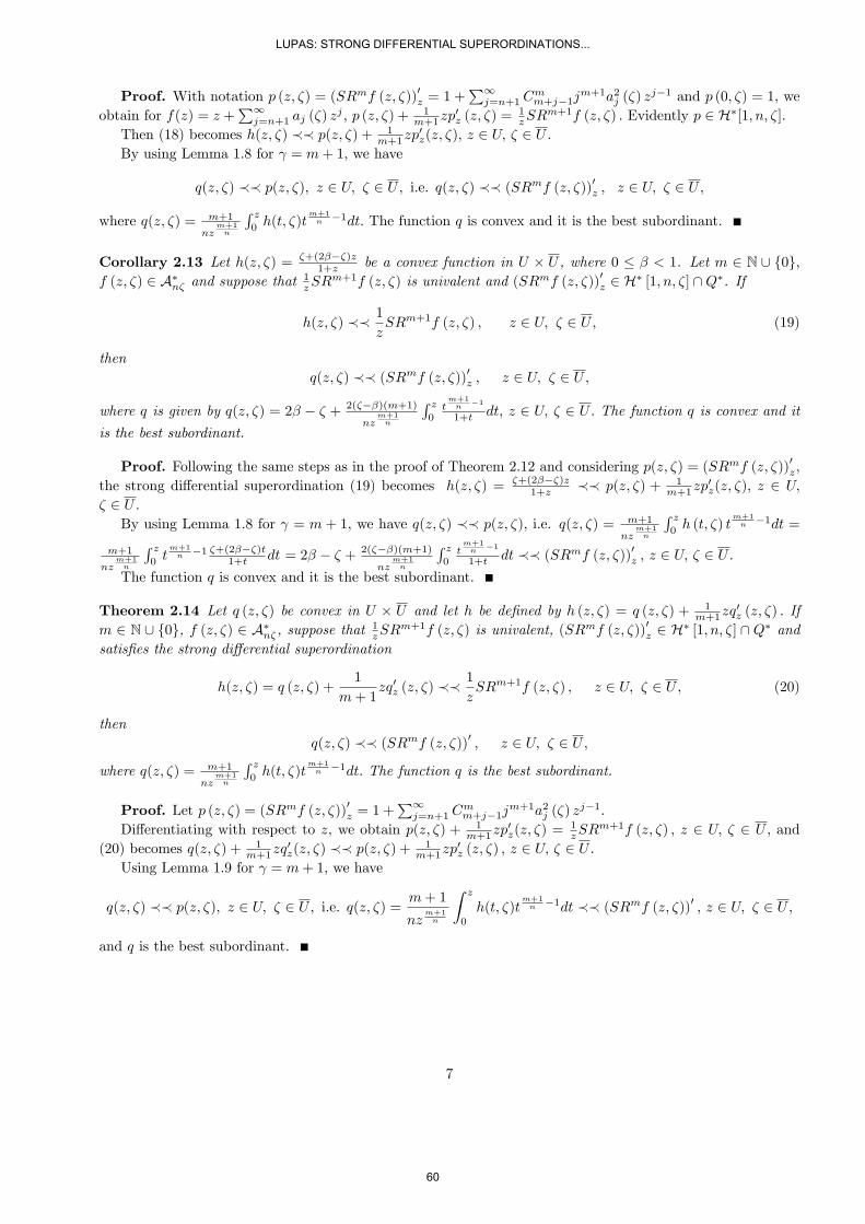
Proof. With notation p (z; ) = (SRmf (z; ))0z = 1 +P1
j=n+1 Cmm+j1j
m+1a2j () zj1 and p (0; ) = 1, we
obtain for f(z) = z +P1
j=n+1 aj () zj ; p (z; ) + 1
m+1zp0z (z; ) =
1zSR
m+1f (z; ) : Evidently p 2 H[1; n; ].Then (18) becomes h(z; ) p(z; ) + 1
m+1zp0z(z; ); z 2 U; 2 U:
By using Lemma 1.8 for = m+ 1, we have
q(z; ) p(z; ); z 2 U; 2 U; i.e. q(z; ) (SRmf (z; ))0z ; z 2 U; 2 U;
where q(z; ) = m+1
nzm+1n
R z0h(t; )t
m+1n 1dt: The function q is convex and it is the best subordinant.
Corollary 2.13 Let h(z; ) = +(2)z1+z be a convex function in U U , where 0 < 1. Let m 2 N [ f0g;
f (z; ) 2 An and suppose that 1zSRm+1f (z; ) is univalent and (SRmf (z; ))0z 2 H [1; n; ] \Q. If
h(z; ) 1
zSRm+1f (z; ) ; z 2 U; 2 U; (19)
thenq(z; ) (SRmf (z; ))0z ; z 2 U; 2 U;
where q is given by q(z; ) = 2 + 2()(m+1)nz
m+1n
R z0tm+1n
1
1+t dt; z 2 U; 2 U: The function q is convex and itis the best subordinant.
Proof. Following the same steps as in the proof of Theorem 2.12 and considering p(z; ) = (SRmf (z; ))0z,the strong di¤erential superordination (19) becomes h(z; ) = +(2)z
1+z p(z; ) + 1m+1zp
0z(z; ); z 2 U;
2 U:By using Lemma 1.8 for = m + 1, we have q(z; ) p(z; ), i.e. q(z; ) = m+1
nzm+1n
R z0h (t; ) t
m+1n 1dt =
m+1
nzm+1n
R z0tm+1n 1 +(2)t
1+t dt = 2 + 2()(m+1)nz
m+1n
R z0tm+1n
1
1+t dt (SRmf (z; ))0z ; z 2 U; 2 U:The function q is convex and it is the best subordinant.
Theorem 2.14 Let q (z; ) be convex in U U and let h be dened by h (z; ) = q (z; ) + 1m+1zq
0z (z; ) : If
m 2 N [ f0g, f (z; ) 2 An , suppose that 1zSRm+1f (z; ) is univalent, (SRmf (z; ))0z 2 H [1; n; ] \Q and
satises the strong di¤erential superordination
h(z; ) = q (z; ) +1
m+ 1zq0z (z; )
1
zSRm+1f (z; ) ; z 2 U; 2 U; (20)
thenq(z; ) (SRmf (z; ))0 ; z 2 U; 2 U;
where q(z; ) = m+1
nzm+1n
R z0h(t; )t
m+1n 1dt: The function q is the best subordinant.
Proof. Let p (z; ) = (SRmf (z; ))0z = 1 +P1
j=n+1 Cmm+j1j
m+1a2j () zj1.
Di¤erentiating with respect to z, we obtain p(z; ) + 1m+1zp
0z(z; ) =
1zSR
m+1f (z; ) ; z 2 U; 2 U; and(20) becomes q(z; ) + 1
m+1zq0z(z; ) p(z; ) + 1
m+1zp0z (z; ) ; z 2 U; 2 U:
Using Lemma 1.9 for = m+ 1, we have
q(z; ) p(z; ); z 2 U; 2 U; i.e. q(z; ) = m+ 1
nzm+1n
Z z
0
h(t; )tm+1n 1dt (SRmf (z; ))0 , z 2 U; 2 U;
and q is the best subordinant.
7
LUPAS: STRONG DIFFERENTIAL SUPERORDINATIONS...
60

References
[1] A. Alb Lupas, G.I. Oros, Gh. Oros, On special strong di¤erential subordinations using S¼al¼agean andRuscheweyh operators, Journal of Computational Analysis and Applications, Vol. 14, 2012 (to appear).
[2] A. Alb Lupas, A note on strong di¤erential subordinations using S¼al¼agean and Ruscheweyh operators, Lib-ertas Mathematica, submitted 2010.
[3] A. Alb Lupas, On special strong di¤erential superordinations using S¼al¼agean and Ruscheweyh operators,submitted 2011.
[4] G.I. Oros, Strong di¤erential superordination, Acta Universitatis Apulensis, Nr. 19, 2009, 101-106.
[5] G.I. Oros, On a new strong di¤erential subordination, (to appear).
8
LUPAS: STRONG DIFFERENTIAL SUPERORDINATIONS...
61

Certain strong di¤erential superordinations using a generalizedS¼al¼agean operator and Ruscheweyh operator
Alina Alb LupasDepartment of Mathematics and Computer Science
University of Oradeastr. Universitatii nr. 1, 410087 Oradea, Romania
Abstract
In the present paper we establish several strong di¤erential superordinations regardind the new opera-tor DRm dened by convolution product of the extended generalized S¼al¼agean operator and Ruscheweyhderivative, DRm : A
! A ; DR
m f (z; ) = (Dm
Rm) f (z; ) ; z 2 U; 2 U; where Rmf(z; ) de-note the extended Ruscheweyh derivative, Dm
f(z; ) is the extended generalized S¼al¼agean operator andAn = ff 2 H(U U); f(z; ) = z + an+1 () z
n+1 + : : : ; z 2 U; 2 Ug; with A1 = A
; is the class ofnormalized analytic functions.
Keywords: strong di¤erential superordination, convex function, best subordinant, extended di¤erential oper-ator, convolution product.2000 Mathematical Subject Classication: 30C45, 30A20, 34A40.
1 Introduction
Denote by U the unit disc of the complex plane U = fz 2 C : jzj < 1g, U = fz 2 C : jzj 1g the closedunit disc of the complex plane and H(U U) the class of analytic functions in U U .Let An = ff 2 H(U U); f(z; ) = z + an+1 () z
n+1 + : : : ; z 2 U; 2 Ug; with A1 = A ; whereak () are holomorphic functions in U for k 2; and H[a; n; ] = ff 2 H(U U); f(z; ) = a + an () z
n +
an+1 () zn+1 + : : : ; z 2 U; 2 Ug; for a 2 C, n 2 N; ak () are holomorphic functions in U for k n:
We also extend the well known di¤erential operators to the new class of analytic functions An introducedin [10].
Denition 1.1 [5] For f 2 A , 0 and m 2 N, the operator Dm is dened by Dm
: A ! A ,
D0f (z; ) = f (z; ) ;
D1f (z; ) = (1 ) f (z; ) + zf 0z(z; ) = Df (z; ) ; :::;
Dm+1 f(z; ) = (1 )Dm
f (z; ) + z (Dm f (z; ))
0z = D (D
m f (z; )) , z 2 U; 2 U:
Remark 1.2 [5] If f 2 A and f(z) = z+P1
j=2 aj () zj, then Dm
f (z; ) = z+P1
j=2 [1 + (j 1)]maj () z
j,z 2 U; 2 U .
Denition 1.3 [4] For f 2 A , m 2 N; the operator Rm is dened by Rm : A ! A ,
R0f (z; ) = f (z; ) ;
R1f (z; ) = zf 0z (z; ) ; :::;
(m+ 1)Rm+1f (z; ) = z (Rmf (z; ))0z +mR
mf (z; ) , z 2 U; 2 U:
1
62
JOURNAL OF APPLIED FUNCTIONAL ANALYSIS, VOL.7, NO’S 1-2,62-68,COPYRIGHT 2012 EUDOXUS PRESS,LLC

Remark 1.4 [4] If f 2 A , f(z; ) = z +P1
j=2 aj () zj, then Rmf (z; ) = z +
P1j=2 C
mm+j1aj () z
j, z 2 U; 2 U:
As a dual notion of strong di¤erential subordination G.I. Oros has introduced and developed the notion ofstrong di¤erential superordinations in [9].
Denition 1.5 [9] Let f (z; ), H (z; ) analytic in U U: The function f (z; ) is said to be strongly su-perordinate to H (z; ) if there exists a function w analytic in U , with w (0) = 0 and jw (z)j < 1; such thatH (z; ) = f (w (z) ; ) ; for all 2 U . In such a case we write H (z; ) f (z; ) ; z 2 U; 2 U:
Remark 1.6 [9] (i) Since f (z; ) is analytic in U U , for all 2 U; and univalent in U; for all 2 U ,Denition 1.5 is equivalent to H (0; ) = f (0; ) ; for all 2 U; and H
U U
f
U U
:
(ii) If H (z; ) H (z) and f (z; ) f (z) ; the strong superordination becomes the usual notion of superor-dination.
Denition 1.7 [6] We denote by Q the set of functions that are analytic and injective on U UnE (f; ),where E (f; ) = fy 2 @U : lim
z!yf (z; ) = 1g; and are such that f 0z (y; ) 6= 0 for y 2 @U UnE (f; ). The
subclass of Q for which f (0; ) = a is denoted by Q (a).
We have need the following lemmas to study the strong di¤erential superordinations.
Lemma 1.8 [6] Let h (z; ) be a convex function with h(0; ) = a and let 2 C be a complex number withRe 0. If p 2 H[a; n; ]\Q; p(z; )+ 1
zp0z(z; ) is univalent in U U and h(z; ) p(z; )+ 1
zp0z(z; );
z 2 U; 2 U; then q(z; ) p(z; ); z 2 U; 2 U; where q(z; ) =
nz n
R z0h (t; ) t
n1dt; z 2 U; 2 U: The
function q is convex and is the best subordinant.
Lemma 1.9 [6] Let q (z; ) be a convex function in U U and let h(z; ) = q(z; ) + 1 zq
0z(z; ); z 2 U; 2 U;
where Re 0. If p 2 H [a; n; ] \Q, p(z; ) + 1 zp
0z(z; ) is univalent in U U and q(z; ) + 1
zq0z(z; )
p(z; )+ 1 zp
0z (z; ) ; z 2 U; 2 U; then q(z; ) p(z; ); z 2 U; 2 U; where q(z; ) =
nz n
R z0h (t; ) t
n1dt;
z 2 U , 2 U: The function q is the best subordinant.
2 Main results
Denition 2.1 [2] Let 0 andm 2 N[f0g. Denote by DRm the operator given by the Hadamard product (theconvolution product) of the extended generalized S¼al¼agean operator Dm
and the extended Ruscheweyh operatorRm, DRm : A ! A ,
DRm f (z; ) = (Dm Rm) f (z; ) :
Remark 2.2 [2] If f 2 A , f(z; ) = z +P1
j=2 aj () zj ; then
DRm f (z; ) = z +P1
j=2 Cmm+j1 [1 + (j 1)]
ma2j () z
j ; z 2 U; 2 U:
Remark 2.3 For = 1 we obtain the Hadamard product SRm ([1], [3], [7], [8]) of the extended S¼al¼ageanoperator Sm and extended Ruscheweyh operator Rm.
Theorem 2.4 Let h (z; ) be a convex function in U U with h (0; ) = 1. Let m 2 N, 0; f (z; ) 2 A ;F (z; ) = Ic (f) (z; ) =
c+2zc+1
R z0tcf (t; ) dt, z 2 U; 2 U , Re c > 2; and suppose that (DRm f (z; ))
0z is
univalent in U U , (DRm F (z; ))0z 2 H [1; 1; ] \Q and
h (z; ) (DRm f (z; ))0z , z 2 U; 2 U; (1)
thenq (z; ) (DRm F (z; ))
0z , z 2 U; 2 U;
where q(z; ) = c+2zc+2
R z0h(t; )tc+1dt: The function q is convex and it is the best subordinant.
2
LUPAS: Using Salagean and Ruscheweyh operators
63
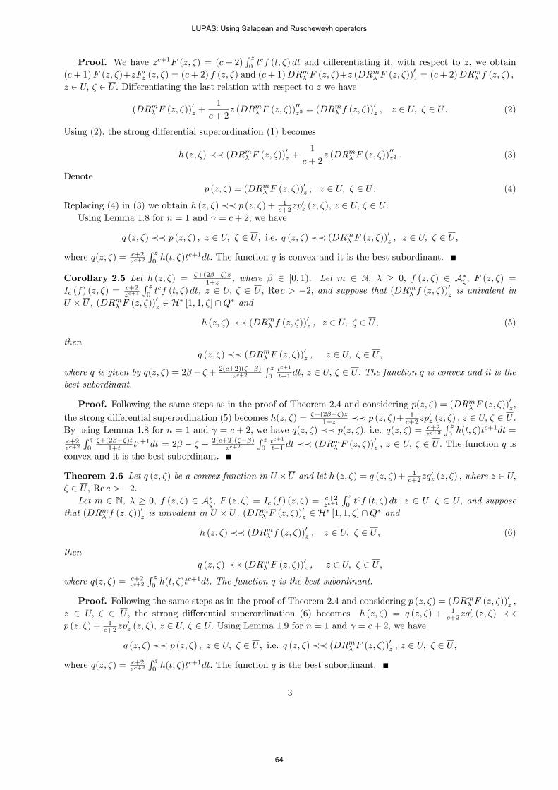
Proof. We have zc+1F (z; ) = (c+ 2)R z0tcf (t; ) dt and di¤erentiating it, with respect to z, we obtain
(c+ 1)F (z; )+zF 0z (z; ) = (c+ 2) f (z; ) and (c+ 1)DRm F (z; )+z (DR
m F (z; ))
0z = (c+ 2)DR
m f (z; ) ;
z 2 U; 2 U: Di¤erentiating the last relation with respect to z we have
(DRm F (z; ))0z +
1
c+ 2z (DRm F (z; ))
00z2 = (DR
m f (z; ))
0z , z 2 U; 2 U: (2)
Using (2), the strong di¤erential superordination (1) becomes
h (z; ) (DRm F (z; ))0z +
1
c+ 2z (DRm F (z; ))
00z2 : (3)
Denotep (z; ) = (DRm F (z; ))
0z ; z 2 U; 2 U: (4)
Replacing (4) in (3) we obtain h (z; ) p (z; ) + 1c+2zp
0z (z; ), z 2 U; 2 U:
Using Lemma 1.8 for n = 1 and = c+ 2; we have
q (z; ) p (z; ) ; z 2 U; 2 U; i.e. q (z; ) (DRm F (z; ))0z , z 2 U; 2 U;
where q(z; ) = c+2zc+2
R z0h(t; )tc+1dt: The function q is convex and it is the best subordinant.
Corollary 2.5 Let h (z; ) = +(2)z1+z ; where 2 [0; 1). Let m 2 N, 0; f (z; ) 2 A ; F (z; ) =
Ic (f) (z; ) =c+2zc+1
R z0tcf (t; ) dt, z 2 U; 2 U; Re c > 2; and suppose that (DRm f (z; ))
0z is univalent in
U U , (DRm F (z; ))0z 2 H [1; 1; ] \Q and
h (z; ) (DRm f (z; ))0z , z 2 U; 2 U; (5)
thenq (z; ) (DRm F (z; ))
0z , z 2 U; 2 U;
where q is given by q(z; ) = 2 + 2(c+2)()zc+2
R z0tc+1
t+1 dt; z 2 U; 2 U: The function q is convex and it is thebest subordinant.
Proof. Following the same steps as in the proof of Theorem 2.4 and considering p(z; ) = (DRm F (z; ))0z,
the strong di¤erential superordination (5) becomes h(z; ) = +(2)z1+z p (z; )+ 1
c+2zp0z (z; ) ; z 2 U; 2 U:
By using Lemma 1.8 for n = 1 and = c + 2, we have q(z; ) p(z; ), i.e. q(z; ) = c+2zc+2
R z0h(t; )tc+1dt =
c+2zc+2
R z0+(2)t
1+t tc+1dt = 2 + 2(c+2)()zc+2
R z0tc+1
t+1 dt (DRm F (z; ))
0z ; z 2 U; 2 U: The function q is
convex and it is the best subordinant.
Theorem 2.6 Let q (z; ) be a convex function in U U and let h (z; ) = q (z; )+ 1c+2zq
0z (z; ) ; where z 2 U;
2 U; Re c > 2:Let m 2 N, 0; f (z; ) 2 A ; F (z; ) = Ic (f) (z; ) =
c+2zc+1
R z0tcf (t; ) dt, z 2 U; 2 U; and suppose
that (DRm f (z; ))0z is univalent in U U , (DRm F (z; ))
0z 2 H [1; 1; ] \Q and
h (z; ) (DRm f (z; ))0z , z 2 U; 2 U; (6)
thenq (z; ) (DRm F (z; ))
0z , z 2 U; 2 U;
where q(z; ) = c+2zc+2
R z0h(t; )tc+1dt: The function q is the best subordinant.
Proof. Following the same steps as in the proof of Theorem 2.4 and considering p (z; ) = (DRm F (z; ))0z ;
z 2 U; 2 U; the strong di¤erential superordination (6) becomes h (z; ) = q (z; ) + 1c+2zq
0z (z; )
p (z; ) + 1c+2zp
0z (z; ), z 2 U; 2 U: Using Lemma 1.9 for n = 1 and = c+ 2; we have
q (z; ) p (z; ) ; z 2 U; 2 U; i.e. q (z; ) (DRm F (z; ))0z , z 2 U; 2 U;
where q(z; ) = c+2zc+2
R z0h(t; )tc+1dt: The function q is the best subordinant.
3
LUPAS: Using Salagean and Ruscheweyh operators
64
Theorem 2.7 Let h (z; ) be a convex function, h(0; ) = 1: Let 0; m 2 N; f (z; ) 2 A and suppose that(DRm f (z; ))
0z is univalent and
DRm f(z;)z 2 H [1; 1; ] \Q. If
h(z; ) (DRm f (z; ))0z ; z 2 U; 2 U; (7)
then
q(z; ) DRm f (z; )
z; z 2 U; 2 U;
where q(z; ) = 1z
R z0h(t; )dt: The function q is convex and it is the best subordinant.
Proof. Consider p (z; ) = DRm f(z;)z =
z+P1
j=2 Cmm+j1[1+(j1)]
ma2j ()zj
z =
1 +P1
j=2 Cmm+j1 [1 + (j 1)]
ma2j () z
j1: Evidently p 2 H[1; 1; ].We have p (z; ) + zp0z (z; ) = (DR
m f (z; ))
0z, z 2 U; 2 U .
Then (7) becomes h(z; ) p(z; ) + zp0z(z; ); z 2 U; 2 U:By using Lemma 1.8 for n = 1 and = 1, we have
q(z; ) p(z; ); z 2 U; 2 U; i.e. q(z; ) DRm f (z; )
z; z 2 U; 2 U;
where q(z; ) = 1z
R z0h(t; )dt: The function q is convex and it is the best subordinant.
Corollary 2.8 Let h(z; ) = +(2)z1+z be a convex function in U U , where 0 < 1. Let 0; m 2 N;
f (z; ) 2 A and suppose that (DRm f (z; ))0z is univalent and
DRm f(z;)z 2 H [1; 1; ] \Q. If
h(z; ) (DRm f (z; ))0z ; z 2 U; 2 U; (8)
then
q(z; ) DRm f (z; )
z; z 2 U; 2 U;
where q is given by q(z; ) = 2 + 2()z ln (1 + z) ; z 2 U; 2 U: The function q is convex and it is the
best subordinant.
Proof. Following the same steps as in the proof of Theorem 2.7 and considering p(z; ) = DRm f(z;)z , the
strong di¤erential superordination (8) becomes h(z; ) = +(2)z1+z p(z; ) + zp0z(z; ); z 2 U; 2 U: By
using Lemma 1.8 for n = 1 and = 1, we have q(z; ) p(z; ), i.e. q(z; ) = 1z
R z0h (t; ) dt = 1
z
R z0+(2)t
1+t dt
= 2+ 2()z ln (1 + z) DRm
f(z;)z ; z 2 U; 2 U: The function q is convex and it is the best subordinant.
Theorem 2.9 Let q (z; ) be convex in U U and let h be dened by h (z; ) = q (z; ) + zq0z (z; ) : If 0,m 2 N, f (z; ) 2 A , suppose that (DRm f (z; ))
0z is univalent,
DRm f(z;)z 2 H [1; 1; ] \ Q and satises the
strong di¤erential superordination
h(z; ) = q (z; ) + zq0z (z; ) (DRm f (z; ))0z ; z 2 U; 2 U; (9)
then
q(z; ) DRm f (z; )
z; z 2 U; 2 U;
where q(z; ) = 1z
R z0h(t; )dt: The function q is the best subordinant.
Proof. Let p (z; ) = DRm f(z;)z =
z+P1
j=2 Cmm+j1[1+(j1)]
ma2j ()zj
z =
1 +P1
j=2 Cmm+j1 [1 + (j 1)]
ma2j () z
j1: Evidently p 2 H[1; 1; ].Di¤erentiating, we obtain p(z; ) + zp0z(z; ) = (DRm f (z; ))
0z ; z 2 U; 2 U; and (9) becomes q(z; ) +
zq0z(z; ) p(z; ) + zp0z (z; ) ; z 2 U; 2 U: Using Lemma 1.9 for n = 1 and = 1, we have
q(z; ) p(z; ); z 2 U; 2 U; i.e. q(z; ) = 1
z
Z z
0
h(t; )dt DRm f (z; )
z; z 2 U; 2 U;
and q is the best subordinant.
4
LUPAS: Using Salagean and Ruscheweyh operators
65
Theorem 2.10 Let h (z; ) be a convex function, h(0; ) = 1: Let 0; m 2 N; f (z; ) 2 A and suppose thatzDRm+1
f(z;)
DRm f(z;)
0zis univalent and DRm+1
f(z;)
DRm f(z;)
2 H [1; 1; ] \Q. If
h(z; ) zDRm+1 f (z; )
DRm f (z; )
0z
; z 2 U; 2 U; (10)
then
q(z; ) DRm+1 f (z; )
DRm f (z; ); z 2 U; 2 U;
where q(z; ) = 1z
R z0h (t; ) dt: The function q is convex and it is the best subordinant.
Proof. Consider p (z; ) = DRm+1 f(z;)
DRm f(z;)
=z+P1
j=2 Cm+1m+j [1+(j1)]
m+1a2j ()zj
z+P1
j=2 Cmm+j1[1+(j1)]
ma2j ()zj =
1+P1
j=2 Cm+1m+j [1+(j1)]
m+1a2j ()zj1
1+P1
j=2 Cmm+j1[1+(j1)]
ma2j ()zj1 : Evidently p 2 H[1; 1; ].
We have p0z (z; ) =(DRm+1
f(z;))0z
DRm f(z;)
p (z; ) (DRm f(z;))
0z
DRm f(z;)
: Then p (z; ) + zp0z (z; ) =zDRm+1
f(z;)
DRm f(z;)
0z:
Then (10) becomes h(z; ) p(z; ) + zp0z(z; ); z 2 U; 2 U: By using Lemma 1.8 for n = 1 and = 1,we have
q(z; ) p(z; ); z 2 U; 2 U; i.e. q(z; ) DRm+1 f (z; )
DRm f (z; ); z 2 U; 2 U;
where q(z; ) = 1z
R z0h (t; ) dt: The function q is convex and it is the best subordinant.
Corollary 2.11 Let h(z; ) = +(2)z1+z be a convex function in U U , where 0 < 1. Let 0, m 2 N;
f (z; ) 2 A and suppose thatzDRm+1
f(z;)
DRm f(z;)
0zis univalent, DR
m+1 f(z;)
DRm f(z;)
2 H [1; 1; ] \Q: If
h(z; ) zDRm+1 f (z; )
DRm f (z; )
0z
; z 2 U; 2 U; (11)
then
q(z; ) DRm+1 f (z; )
DRm f (z; ); z 2 U; 2 U;
where q is given by q(z; ) = 2 + 2()z ln (1 + z) ; z 2 U; 2 U: The function q is convex and it is the
best subordinant.
Proof. Following the same steps as in the proof of Theorem 2.10 and considering p(z; ) = DRm+1 f(z;)
DRm f(z;)
, the
strong di¤erential superordination (11) becomes h(z; ) = +(2)z1+z p(z; ) + zp0z(z; ); z 2 U; 2 U: By
using Lemma 1.8 for n = 1 and = 1, we have q(z; ) p(z; ), i.e. q(z; ) = 1z
R z0h (t; ) dt = 1
z
R z0+(2)t
1+t dt
= 2+ 2()z ln (1 + z) DRm+1
f(z;)
DRm f(z;)
; z 2 U; 2 U: The function q is convex and it is the best subordinant.
Theorem 2.12 Let q (z; ) be convex in U U and let h be dened by h (z; ) = q (z; ) + zq0z (z; ) : If 0;m 2 N, f (z; ) 2 A , suppose that
zDRm+1
f(z;)
DRm f(z;)
0zis univalent, DR
m+1 f(z;)
DRm f(z;)
2 H [1; 1; ] \ Q and satisesthe strong di¤erential superordination
h(z; ) = q (z; ) + zq0z (z; ) zDRm+1 f (z; )
DRm f (z; )
0z
; z 2 U; 2 U; (12)
then
q(z; ) DRm+1 f (z; )
DRm f (z; ); z 2 U; 2 U;
where q(z; ) = 1z
R z0h (t; ) dt: The function q is the best subordinant.
5
LUPAS: Using Salagean and Ruscheweyh operators
66

Proof. Let p (z; ) = DRm+1 f(z;)
DRm f(z;)
=z+P1
j=2 Cm+1m+j [1+(j1)]
m+1a2j ()zj
z+P1
j=2 Cmm+j1[1+(j1)]
ma2j ()zj =
1+P1
j=2 Cm+1m+j [1+(j1)]
m+1a2j ()zj1
1+P1
j=2 Cmm+j1[1+(j1)]
ma2j ()zj1 :
Evidently p 2 H[1; 1; ].
Di¤erentiating with respect to z, we obtain p(z; ) + zp0z(z; ) =zDRm+1
f(z;)
DRm f(z;)
0z; z 2 U; 2 U; and (12)
becomes q(z; )+ zq0z(z; ) p(z; )+ zp0z (z; ) ; z 2 U; 2 U: Using Lemma 1.9 for n = 1 and = 1, we have
q(z; ) p(z; ); z 2 U; 2 U; i.e. q(z; ) = 1
z
Z z
0
h (t; ) dt DRm+1 f (z; )
DRm f (z; ); z 2 U; 2 U;
and q is the best subordinant.
Theorem 2.13 Let h (z; ) be a convex function, h(0; ) = 1: Let 0; m 2 N; f (z; ) 2 A and suppose thatm+1
(m+1)zDRm+1 f (z; ) m(1)
(m+1)zDRm f (z; ) is univalent and (DR
m f (z; ))
0z 2 H [1; 1; ] \Q. If
h(z; ) m+ 1
(m+ 1) zDRm+1 f (z; ) m (1 )
(m+ 1) zDRm f (z; ) ; z 2 U; 2 U; (13)
thenq(z; ) (DRm f (z; ))
0z ; z 2 U; 2 U;
where q(z; ) = m+1
zm+1
R z0h (t; ) t
(m1)+1 dt: The function q is convex and it is the best subordinant.
Proof. With notation p (z; ) = (DRm f (z; ))0z = 1 +
P1j=2 C
mm+j1 [1 + (j 1)]
mja2j () z
j1 andp (0; ) = 1, we obtain for f(z; ) = z +
P1j=2 aj () z
j ;
p (z; ) + zp0z (z; ) =m+1z DR
m+1 f (z; )
m 1 + 1
(DRm f (z; ))
0z
m(1)z DRm f (z; ) and
p (z; ) + m+1zp
0z (z; ) =
m+1(m+1)zDR
m+1 f (z; ) m(1)
(m+1)zDRm f (z; ) : Evidently p 2 H[1; 1; ].
Then (13) becomes h(z; ) p (z; ) + m+1zp
0z (z; ) ; z 2 U; 2 U: By using Lemma 1.8 for n = 1 and
= m+ 1 , we have
q(z; ) p(z; ); z 2 U; 2 U; i.e. q(z; ) (DRm f (z; ))0z ; z 2 U; 2 U;
where q(z; ) = m+1
zm+1
R z0h (t; ) t
(m1)+1 dt: The function q is convex and it is the best subordinant.
Corollary 2.14 Let h(z; ) = +(2)z1+z be a convex function in U U , where 0 < 1. Let 0, m 2 N;
f (z; ) 2 A and suppose that m+1(m+1)zDR
m+1 f (z; ) m(1)
(m+1)zDRm f (z; ) is univalent, (DR
m f (z; ))
0z 2
H [1; 1; ] \Q: If
h(z; ) m+ 1
(m+ 1) zDRm+1 f (z; ) m (1 )
(m+ 1) zDRm f (z; ) ; z 2 U; 2 U; (14)
thenq(z; ) (DRm f (z; ))
0z ; z 2 U; 2 U;
where q is given by q(z; ) = 2 + 2()(m+1)z
m+1
R z0tm+1
1
1+t dt; z 2 U; 2 U: The function q is convex andit is the best subordinant.
Proof. Following the same steps as in the proof of Theorem 2.13 and considering p(z; ) = (DRm f (z; ))0z,
the strong di¤erential superordination (14) becomes h(z; ) = +(2)z1+z p(z; )+zp0z(z; ); z 2 U; 2 U: By
using Lemma 1.8 for n = 1 and = m+1 , we have q(z; ) p(z; ), i.e. q(z; ) = m+1
zm+1
R z0h (t; ) t
(m1)+1 dt
= m+1
zm+1
R z0t(m1)+1
+(2)t
1+t dt = 2 + 2()(m+1)z
m+1
R z0tm+1
1
1+t dt (DRm f (z; ))0z ; z 2 U; 2 U:
The function q is convex and it is the best subordinant.
6
LUPAS: Using Salagean and Ruscheweyh operators
67

Theorem 2.15 Let q (z; ) be convex in U U and let h be dened by h (z; ) = q (z; ) + m+1zq
0z (z; ),
0; m; n 2 N. If f (z; ) 2 An ; suppose that m+1(m+1)zDR
m+1 f (z; ) m(1)
(m+1)zDRm f (z; ) is univalent and
(DRm f (z; ))0z 2 H [1; 1; ] \Q and satises the strong di¤erential superordination
h(z; ) = q (z; ) +
m+ 1zq0z (z; ) (15)
m+ 1
(m+ 1) zDRm+1 f (z; ) m (1 )
(m+ 1) zDRm f (z; ) ; z 2 U; 2 U;
thenq(z; ) (DRm f (z; ))
0z ; z 2 U; 2 U;
where q(z; ) = m+1
zm+1
R z0h (t; ) t
(m1)+1 dt: The function q is the best subordinant.
Proof. Let p (z; ) = (DRm f (z; ))0= 1 +
P1j=2 C
mm+j1 [1 + (j 1)]
mja2j () z
j1.Di¤erentiating, we obtain
p (z; ) + zp0z (z; ) =m+1z DR
m+1 f (z; )
m 1 + 1
(DRm f (z; ))
0z
m(1)z DRnf (z; ) and
p (z; ) + m+1zp
0z (z; ) =
m+1(m+1)zDR
m+1 f (z; ) m(1)
(m+1)zDRm f (z; ) ; z 2 U; 2 U; and (15) becomes
q(z; ) + m+1zq
0z(z; ) p(z; ) +
m+1zp0z (z; ) ; z 2 U; 2 U: Using Lemma 1.9 for n = 1 and = m+ 1
,
we have q(z; ) p(z; ); z 2 U; 2 U; i.e. q(z; ) = m+1
zm+1
R z0h (t; ) t
(m1)+1 dt (DRm f (z; ))
0z, z 2 U;
2 U; and q is the best subordinant.
References
[1] A. Alb Lupas, Certain strong di¤erential subordinations using S¼al¼agean and Ruscheweyh operators, Ad-vances in Applied Mathematical Analysis, Volume 6, Number 1 (2011), 2734.
[2] A. Alb Lupas, A note on strong di¤erential subordinations using a generalized S¼al¼agean operator andRuscheweyh operator, Bulletin of Mathematical Analysis and Applications, submitted 2010.
[3] A. Alb Lupas, A note on strong di¤erential subordinations using S¼al¼agean and Ruscheweyh operators,Libertas Mathematica, submitted 2010.
[4] A. Alb Lupas, G.I. Oros, Gh. Oros, On special strong di¤erential subordinations using S¼al¼agean andRuscheweyh operators, Journal of Computational Analysis and Applications, Vol. 14, 2012 (to appear).
[5] A. Alb Lupas, On special strong di¤erential subordinations using a generalized S¼al¼agean operator andRuscheweyh derivative, submitted 2011.
[6] A. Alb Lupas, On special strong di¤erential superordinations using S¼al¼agean and Ruscheweyh operators,submitted 2011.
[7] A. Alb Lupas, Certain strong di¤erential superordinations using S¼al¼agean and Ruscheweyh operators, sub-mitted 2011.
[8] A. Alb Lupas, A note on strong di¤erential superordinations using S¼al¼agean and Ruscheweyh operators,submitted 2011.
[9] G.I. Oros, Strong di¤erential superordination, Acta Universitatis Apulensis, Nr. 19, 2009, 101-106.
[10] G.I. Oros, On a new strong di¤erential subordination, (to appear).
7
LUPAS: Using Salagean and Ruscheweyh operators
68
1
A NEW FIXED POINT THEOREM FOR m MAPINGS ON m COMPLETE METRIC SPACES
Luljeta Kikina and Kristaq Kikina
Department of Mathematics and Computer Science Faculty of Natural Sciences, University of Gjirokastra
Albania [email protected], [email protected]
Abstract: A new fixed point theorem for m N∈ mappings, satisfying implicit relations, was proved. This result generalizes and unifies several of well-known fixed point theorems for one, two and three mappings and extends then to an arbitrary number mof mappings. Keywords: Cauchy sequence, complete metric space, fixed point, implicit relation. Mathematics Subject Classification: 47H10, 54H25
1. INTRODUCTION
In [1], [2], [8], [11] etc, are proved fixed point theorems on metric spaces for mappings satisfying implicit relations. In this paper, we will prove a related fixed point theorem for m mappings on m metric spaces, 1m− of mappings must be continuous. This result generalizes and unifies the theorems of Rhoades [10], Banach [3], Kannan [7], Bianchini [4], Reich [9], Fisher [5], Jain et al [6], etc. and in the same time, it extends them for an arbitrary number mof mappings.
These generalizations and unifications have been done using a wide class of implicit relations. In [10], [5] and [6], the following theorems are proved.
Theorem 1.1 (Rhoades [10]) Let ( , )X d be a complete metric space and XXT →: a
self map of X. If for some [0,1)c∈ we have
( , ) max ( , ), ( , ), ( , )d Tx Ty c d x y d x Tx d y Ty≤
for all ,x y X∈ , then T has a unique fixed point α in X.
Theorem 2.2 Fisher [5]) Let ( , ) ( , )X d and Y ρ are complete metric spaces and
XYRYXS →→ : , : be two maps, at least one of them being continuous. If for some
(0,1)c∈ the following inequalities are satisfied:
( ) ( ) ( ) ( ) ( ), ' max , ' , , , ', ' , , ' d RSx RSx c d x x d x RSx d x RSx Sx Sxρ≤
( ) ( ) ( ) ( ) ( ), ' max , ' , , , ', ' , , ' SRy SRy c y y y SRy y SRy d Ry Ryρ ρ ρ ρ≤
69
JOURNAL OF APPLIED FUNCTIONAL ANALYSIS, VOL.7, NO’S 1-2,69-80,COPYRIGHT 2012 EUDOXUS PRESS,LLC

2
for all , ' ; , 'x x X y y Y∈ ∈ , then RS has a unique fixed point X∈α and SR has a unique fixed
point Y∈β . Moreover, βα =S and. αβ =R
Theorem 1.3 ( Jain et al [6] ) Let ( , ), ( , )X d Y ρ and ( , )Z σ be complete metric
spaces. If T is a continuous mapping of X into Y , S is a continuous mapping of Y into Z and R is a mapping of Z into X satisfying the inequalities
( , ) max ( , ), ( , ), ( , ) ( , ), ( , )( , ) max ( , ), ( , ), ( , ) ( , ), ( , )( , ) max ( , ), ( , ), ( , ), ( , ),
d RSTx RSTx c d x x d x RSTx d x RSTx Tx Tx STx STx
TRSy TRSy c y y y TRSy y TRSy Sy Sy d RSy RSy
STRz STRz c z z z STRz z STRz d Rz Rz
ρ σρ ρ ρ ρ σσ σ σ σ ρ
′ ′ ′ ′ ′ ′≤′ ′ ′ ′ ′ ′≤′ ′ ′ ′ ′≤ ( , )TRz TRz′
for all , ; , ,x x X y y Y and z z Z′ ′ ′∈ ∈ ∈ where 0 < 1c≤ . Then RST has a unique fixed point u in X , TRS has a unique fixed point v in Y and STR has a unique fixed point w in Z . Further, = , =Tu v Sv w and Rw u= .
2. MAIN RESULTS Before stating the main theorem we define new classes implicit functions, whose role will be crucial. Let [0, )R+ = +∞ . We denote by kΦ , for 4k ≥ , the set of all functions with k variables
: kR Rϕ + → satisfying the properties: (a). ϕ is upper semi-continuous in each coordinate variable 1 2, ,..., kt t t (b). If 1 2 4( , , , , , ,..., ) 0ku v v u v v vϕ − ≤ or 1 2 4( , , , , , ,..., ) 0ku v u v v v vϕ − ≤ or 1 2 4( , , , , , ,..., ) 0ku u v v v v vϕ − ≤ , for all 1 2 4, , , ,..., 0ku v v v v− ≥ , then there exists a real constant 0 1c≤ < such that 1 2 4max , , ,..., ku c v v v v−≤ .
Every such function will be called a kΦ -function with constant c. Note: If 1 2k k< , then
1 2k kΦ ⊂ Φ . In the case 4k = , we have 1 2 4( , , , , , ,..., ) ( , , , )ku v v u v v v u v v uϕ ϕ− = and 1 2 4max , , ,..., kv v v v v− = Example 2.1 The function 1 2 1 2 3( , ,..., ) max , ,..., p p p p
k kt t t t c t t tϕ = − , where 0 1c≤ < and 0p > , is kΦ -function with constant c. Proof: (a) is clear since ϕ is continuous. Suppose that 1 2 4, , , ,..., 0ku v v v v− ≥ and then
1 2 4 1 2 4
1 2 4
( , , , , , ,..., ) max , , , , ,...,
max , , , ,..., 0
p p p p p p pk k
p p p p p pk
u v v u v v v u c v v u v v v
u c u v v v v
ϕ − −
−
= − =
= − ≤
If 1 2 4max , , ,..., ,p p p p pku v v v v−≥ then 1 2 4max , , , ,..., p p p p p p p p
ku c u v v v v cu u−≤ = < , a contradiction. Therefore,
1 2 4 1 1 2 4max , , ,..., max , , ,..., p p p p pk ku c v v v v and so u c v v v v− −≤ ≤
where 1 1pc c= < . Similarly, if 1 2 4( , , , , , ,..., ) 0ku v u v v v vϕ − ≤ or
KIKINA: FIXED POINT THEOREM
70

3
1 2 4( , , , , , ,..., ) 0ku u v v v v vϕ − ≤ , then 1 1 2 4max , , ,..., ku c v v v v−≤ . The proof of (b) is completed.
Example 2.2 The function1
1 2 1 2 2 3 3( , ,..., ) = ( ... ) pp p pk k kt t t t a t a t a tϕ − + + + , where 0p >
and2
0 , 1, 2,3,...,k
i ii
a a i k=
≤ < =∑ , is kΦ -function with constant 2
k
ii
c a=
=∑
Proof: (a) is clear since ϕ is continuous. Suppose that 1 2 4, , , ,..., 0ku v v v v− ≥ and then
1
1 2 4 2 3 4 5 1 4( , , , , , ,..., ) ( ... ) 0pp p p p pk k ku v v u v v v u a v a v a u a v a vϕ − −= − + + + + ≤
If 1 2 4max , , ,..., ,p p p p pku v v v v−≥ then
1 1
1 1
2 3 4 5 1 4 2 3 4 5
2 3 4 2 3 4
( ... ) ( ... )
[( ... ) ] ( ... ) ,
p p
p p
p p p p p p p p p pk k k
pk k
u a v a v a u a v a v a u a u a u a u a u
a a a a u a a a a u cu u
−≤ + + + + + ≤ + + + + =
= + + + + = + + + + = <
a contradiction, where 1
2 3 4( ... ) 1p
kc a a a a= + + + + < . Therefore, 1
2 3 4 1 2 4[( ... ) max , , ,..., ] pp p p pk ku a a a a v v v v−≤ + + + + 1 2 4max , , ,..., kc v v v v−= . Similarly,
if 1 2 4( , , , , , ,..., ) 0ku v u v v v vϕ − ≤ or 1 2 4( , , , , , ,..., ) 0ku u v v v v vϕ − ≤ , then
1 1 2 4max , , ,..., ku c v v v v−≤ . The proof of (b) is completed.
We denote by kF the set of all continuous functions with k variables : kf R R+ → satisfying the properties: (a’). f is non decreasing in respect with each variable. (b’). ( , ,..., ) ,f t t t t t R+≤ ∈ Every such function will be called a kF -function.
Denote = 1, 2,..., kI k . Some examples of kF -function are as follows: 1. 1 2 1 2( , ,..., ) = max , ,..., k kf t t t t t t
2. 12
1 2 1 2 2 3 1 1( , ,..., ) = [max , ,..., , ]k k k kf t t t t t t t t t t t−
3. 1
1 2 1 2( , ,..., ) = [max , ,..., ] , 0pp p pk kf t t t t t t p >
4. 1 1 2 21 2
1 2
...( , ,..., ) =...
k kk
k
a t a t a tf t t t
a a a
+ + ++ + +
, where 0p > and 0ia ≥
The following relationship between 1k−F -functions and kΦ -functions holds:
Lemma 2.3 If 1kf −∈F and 0 1c≤ < , then the function 1 2 1 2 3( , ,..., )= ( , ,..., )k kt t t t cf t t tϕ − is
kΦ -function with constant c Proof. (a) is clear since ϕ is continuous. Suppose that 1 2 4, , , ,..., 0ku v v v v− ≥ and then 1 2 4 1 4( , , , , , ,..., ) ( , , , ,..., )k ku v v u v v v u cf v v u v v oϕ − −= − ≤ (*) We have 1 2 4max , , ,..., ku v v v v−≤ since in contrary, ( if 1 2 4max , , ,..., ku v v v v−> ), by using the properties of f we get: 1 4( , , , ,..., ) ( , ,..., )kf v v u v v f u u u u− ≤ ≤ and by (*) it follows u cu u≤ < , a contradiction. Therefore, after replacing the coordinates of the point
KIKINA: FIXED POINT THEOREM
71

4
1 2 4( , , , , ,..., )kv v u v v v− by 1 2 4max , , ,..., kv v v v − and using the properties of f we get
1 2 4max , , ,..., ku c v v v v−≤ . Similarly, if 1 2 4( , , , , , ,..., ) 0ku v u v v v vϕ − ≤ or
1 2 4( , , , , , ,..., ) 0ku u v v v v vϕ − ≤ , then 1 2 4max , , ,..., ku c v v v v−≤ . The proof of (b) is completed. The above lemma gives us the possibility to establish other functions of type kΦ :
Example 2.4 1
21 2 1 2 3 3 4 1( , ,..., ) = [max , ,..., ]k k kt t t t c t t t t t tϕ −− , where 0 1c≤ < .
Example 2.5 ( ) 2 31 2 1
..., ,...,1
kk
t t tt t t t c
kϕ + + += −
−, where 0 1c≤ < etc.
Now, we prove the following theorem for m mappings on m metric spaces. Theorem 2.6 Let ( , )i iX d be m complete metric spaces and iT m mappings such
that 1 1: 1, 2,..., 1, :i i i m mT X X for i m T X X+→ = − → and from which ( 1)m − are continuous. If satisfying the inequalities:
( ) ( ) ( )( ) ( ) ( )( )
' '1 1 2 1 1 1 2 1 1 1 1 1 1 1 1 1 1
' ' ' '1 1 1 1 1 1 2 1 1 1 1 3 2 1 1 2 1 1
'1 2 1 1 1 2 1 1
... , ... , , , , ... ,
, ... , , , d , ,..., 0
... , ...
m m m m m m
m m
m m m m m
d T T T T x T T T T x d x x d x T T T x
d x T T T x d T x T x T T x T T x
d T T T x T T T x
ϕ− − −
−
− − − −
≤
(1)
for all '1 1 1,x x X∈
( ) ( ) ( )( ) ( ) ( )( ) ( )
' '2 1 3 2 2 1 3 2 2 2 2 2 2 2 1 2 2
' ' ' '2 2 2 1 2 2 3 2 2 2 2 4 3 2 2 3 2 2
' '1 2 2 2 1 2 2 2 1 1 2 2 1 2 2
... , ... , , , , ... ,
, ... , , , , ,..., 0
... , ... , ... , ...
m m m
m
m m m m m m m m m
d TT T T x TT T T x d x x d x TT T x
d x TT T x d T x T x d T T x T T x
d T T T x T T T x d T T T x T T T x
ϕ
− − − − − −
≤
(2)
for all '2 2 2,x x X∈ , in general
( ) ( )( ) ( )
( ) ( )
' '1 2 1 1 1 2 1 1
' '1 2 1 1 1 2 1 1
' '1 1 2 1 2 1 1
... ... , ... ... , , ,
, ... ... , , ... ... ,
, ,..., ... , ... , ...
i i i m m i i i i m m i i i i i
i i i i m m i i i i i i m m i i
i
i i i i i m m m i i m m i i m m
d T T TT T T x T T TT T T x d x x
d x T T TT T T x d x T T TT T T x
d T x T x d T T T x T T T x d T T Tϕ
− − − − − −
− − − − − −
+ − − − − −( )( ) ( )
'1
' '2 1 1 1 1 1 2 3 1 1 2 3 1 1
, ... ,
... , ... ,..., ... ... , ... ...
i i m m i i
m m i i m m i i i i i m m i i i i m m i i
x T T T x
d TT T T x TT T T x d T T TT T T x T T TT T T x
−
− − − − − − − − −
(i)
for all ',i i ix x X∈ for 3,..., 1i m= − , and
KIKINA: FIXED POINT THEOREM
72

5
( ) ( ) ( )( ) ( ) ( )
( )
' '1 2 1 1 2 1 1 2 1
' ' ' '1 2 1 1 2 1 1
'1 2 3 1 2 3 1
... , ... , , , , ... ,
, ... , , , , ,...,
... , ...
m m m m m m m m m m m m m m m m m m
m m m m m m m m m m m m m m m
m m m m m m m m m
d T T TT x T T TT x d x x d x T T TT x
d x T T TT x d T x T x d TT x TT x
d T T TT x T T TT x
ϕ− − − − − −
− −
− − − − −
(m)
for all ',m m mx x X∈ , where 3i mϕ +∈Φ for 1,2,...,i m= .
Then the maps
1 1...m mT T T− , 1 1 2...m mTT T T− , …, 1 2 1 1... ...i i m m iT T TT T T− − − ,…, 1 2 1...m m mT T TT− −
have unique fixed point 1 1,Xα ∈ 2 2 ,Xα ∈ …, ,i iXα ∈ …, m mXα ∈ , respectively.
Further,
1 11,..., 1i i i m mT for i m and Tα α α α+= = − =
Proof. Let (1 )0x be an arbitrary point in 1X . We define the sequences
(1 ) ( 2 ) ( ) ( )1 2, , . . . , , . . . , , , . . . , , . . . ,i m
n n n n i mx x x x in X X X X respectively, as
follows: (1) (1) (2) (1) ( ) ( 1) ( ) ( 1)
1 1 0 1 1 1 1( ... ) , , ..., , ..., ,n i i m mn m m n n n i n n m nx T T T x x T x x T x x T x n N− −
− − − −= = = = ∈
We prove that ( )inx are Cauchy sequences for i=1, 2… m. Denote
( ) ( ) ( )1( , ) , 1, 2 , ..., .i i i
n i n nd d x x i m+= =
We will assume that ( ) ( )1
i in nx x +≠ for all n. Otherwise, if (1) (1)
1n nx x += for some n, then ( ) ( )
1 2i i
n nx x+ += for i=2, 3,…, m and we could put ( )1
ii nxα += .
Applying the inequality (2) for (2) (2)2 1 2n nx x and x x− ′= = , we have:
( ) ( ) ( )( ) ( ) ( )( )
( 2 ) ( 2 ) ( 2 ) ( 2 ) ( 2 ) ( 2 )2 1 3 2 1 1 2 2 1 2 1 1 2 1
( 2 ) ( 2 ) ( 2 ) ( 2 ) ( 2 ) ( 2 )2 2 1 2 3 2 1 2 4 3 2 1 3 2
( 2 ) ( 2 )1 2 2 1 1 2 2 1
... , ... , , , , ... ,
, ... , , , , , ...,
... , ... ,
m n m n n n n m n
n m n n n n n
m m m n m m n m m
d T T T T x T T T x d x x d x T T T x
d x T T T x d T x T x d T T x T T x
d T T T x T T T x d T T
ϕ− − − −
− −
− − − − − ( )( )
( 2 ) ( 2 )1 2 1 1 2
( 2 ) ( 2 ) ( 2 ) ( 2 ) (3) ( 4 ) ( ) (1)2 1 1 1 1 1 1
... , ...
, , , , , , ..., , 0
n m m n
mn n n n n n n n
T x T T T x
d d d d d d d dϕ
− − −
− − − − − −
=
= ≤
and from (b), we have (2) (2) (3) (4) ( ) (1)1 1 1 1 1max , , ,..., ,m
n n n n n nd c d d d d d− − − − −≤ or
(2) (1) (2) (3) (4) ( )1 1 1 1 1max , , , ,..., m
n n n n n nd c d d d d d− − − − −≤ (2’)
We have denoted by 1 2max , ,..., mc c c c= , where ic is the constant of kΦ -function iϕ .
Applying inequality (i) for ( ) ( )1
i ii n i nx x and x x− ′= = , we obtain:
KIKINA: FIXED POINT THEOREM
73
6
( ) ( )( ) ( ) ( )
( ) ( ) ( ) ( )1 2 1 1 1 1 2 1 1 1
( ) ( ) ( ) ( ) ( ) ( )1 1 2 1 1 1 1 2 1 1 1 1
(2 1 1
... ... , ... ... , , ,
, ... ... , , ... ... , , ,
i i i ii i i m m i n i i m m i n i n n
i i i i i ii n i i m m i n i n i i m m i n i i n i n
ii i i i n
d T T TT T T x T T TT T T x d x x
d x T T TT T T x d x T T TT T T x d T x T x
d T T xϕ
− − − − − − − −
− − − − − − − − + −
+ + −( ) ( )( ) ( )
) ( ) ( ) ( )1 1 2 1 1 2
( ) ( ) ( ) ( )1 1 1 1 2 1 1 1 1 1
( )1 2 3 1 1 1 2 3 1 1
, ,..., ... , ... ,
... , ... , ... , ... ,...,
... ... , ... .
i i ii i n m m m i n m m i n
i i i im m i n m m i n m m i n m m i n
ii i i m m i n i i m m
T T x d T T T x T T T x
d T T T x T T T x d TT T T x TT T T x
d T T TT T T x T T TT T
+ − − − − −
− − − − − −
− − − − − − − −( )( ).. ii nT x
=
( ) ( ) ( ) ( ) ( 1) ( 2) ( ) (1) (2) ( 1)
1 1 1 1 1 1( , , , , , ,..., , , ,..., ) 0i i i i i i m ii n n n n n n n n n nd d d d d d d d d dϕ + + −
− − − − − −= ≤
and from (b), we have
( ) ( 1) ( 2) ( ) (1) (2) (3) ( 1)1 1 1 1 1max( , , ,..., , , , ,..., )i i i i m i
n n n n n n n n nd c d d d d d d d d+ + −− − − − −≤ (*)
By (*), for i=3 we have: 3 (3) (4) ( ) (1) (2)
1 1 1 1max( , ,..., , , )mn n n n n nd c d d d d d− − − −≤
By this inequality and (2’) it follows:
(3) (1) (2) (3) (4) ( )1 1 1 1 1max , , , ,..., m
n n n n n nd c d d d d d− − − − −≤ (3’)
In similar way, for i=4,5,…,m-1 and by the inequalities (2’),(3’),...,((i-1)’) we get:
( ) (1) (2) (3) (4) ( )1 1 1 1 1max , , , ,..., 2,3,..., 1i m
n n n n n nd c d d d d d i m− − − − −≤ = − (i)
Applying inequality (m) for ( ) ( )1
m mm n m nx x and x x− ′= = , we have:
( ) ( )( ) ( ) ( )
( )
1 2 1 1 1 2 1 1 1 1 2 1 1
1 2 1 1 1 2 1 1 1
1 2 3 1 1 2 3 1
... , ... , ( , ), , ... ,
, ... , , , , ,...,
... , ...
m m m m m mm m m m n m m m n m n n m n m m m n
m m m m m mm m n m m m n m n m n m n m n
m mm m m m n m m m n
d T T TT x T T TT x d x x d x T T TT x
d x T T TT x d T x T x d TT x TT x
d T T TT x T T TT x
ϕ− − − − − − − − − −
− − − −
− − − − − −
=
( ) ( ) ( ) ( ) (1) (2) (3) ( 1)1 1 1( , , , , , , ,..., )m m m m m
m n n n n n n n nd d d d d d d dϕ −− − −=
and from (b), we have: ( ) (1) (2) (3) ( 1)
1 1max( , , , ,..., )m m mn n n n n nd c d d d d d −
− −≤
By this inequality and by (2’),(3’),…, ((m-1)’) it follows: ( ) (1) (2) (3) ( )
1 1 1 1max( , , ,..., )m mn n n n nd c d d d d− − − −≤ (m’)
Applying inequality (1) for (1) (1)1 1 1n nx x and x x− ′= = , we have:
KIKINA: FIXED POINT THEOREM
74

7
( ) ( ) ( )( ) ( ) ( )
(1) (1) (1) (1) (1) (1)1 1 2 1 1 1 2 1 1 1 1 1 1 1 1
(1) (1) (1) (1) (1) (1)1 1 1 1 2 1 1 1 3 2 1 1 2 1
(1) (1 2 1 1 2 1
... , ... , , , , ... ,
, ... , , , d , ,...,
... , ...
m m n m m n n n n m m n
n m m n n n n n
m m m n m m n
d T T T T x T T T T x d x x d x T T T x
d x T T T x d T x T x T T x T T x
d T T T x T T T x
ϕ− − − − − − −
− − −
− − − −( )1)
(1) (1) (1) (1) (2) (3) ( )1 1 1( , , , , , ,..., ) 0m
n n n n n n nd d d d d d dϕ − −
=
= ≤
and from (b) we have:
(1) (1) (2) (3) ( )1max , , ,..., m
n n n n nd c d d d d−≤
By this inequality and by (2’),(3’),…,(m’) it follows: (1) (1) (2) (3) ( )
1 1 1 1max , , ,..., mn n n n nd c d d d d− − − −≤ (1’)
It now follows from (1’),(2’),…,(m’) that for large enough m ( ) ( ) ( ) (1) (2) (3) ( )
1 1 1 1 12 (1) (2) (3) ( )
2 2 2 23 (1) (2) (3) ( )
3 3 3 3
1 (1) (2) (3) ( ) 11 1 1 1
( , ) max , , ,...,
max , , ,...,
max , , ,..., ...
max , , ,...,
i i i mn i n n n n n n
mn n n n
mn n n n
n m n
d d x x c d d d d
c d d d d
c d d d d
c d d d d c l
+ − − − −
− − − −
− − − −
− −
= ≤
≤
≤
≤ =
where (1) (2) (3) ( )
1 1 1 1max , , ,..., ml d d d d=
Since 0 1c≤ < , it follows that ( ) inx are Cauchy sequences with the limits
1, 2,..., .i iin X for i mα =
Now suppose that iT for 1,2,..., 1i m= − are continuous, we have
(2) (1)1 1 1 1 2lim limn n
n nx T x Tα α−→∞ →∞
= ⇒ = and ( 1) ( )1 1lim limi i
n i n i i in n
x T x Tα α++ +→∞ →∞
= ⇒ =
for 2,3,..., 1i m= −
Later we will show that 1m mT α α= .
To prove that 1α is a fixed point of 1 1...m mT T T−
Using the inequality (1) for ' (1)1 1 1 1nx and x xα −= = , we obtain:
( ) ( ) ( ) ( )( ) ( ) ( )
(1) (1) (1) (1)1 1 2 1 1 1 1 1 1 1 1 1 1 1 1
1 (1) (1) (1)2 1 1 1 1 3 2 1 1 2 1 1 1 2 1 1 1 2 1 1
... , , , , , ... , , ,0
, , d , ,..., ... , ...
m m n n m m n n
n n m m m m m n
d T T T T x d x d T T T d x x
d T T x T T TT x d T T T T T T x
α α α αϕ
α α α− − − −
− − − − − − −
≤
Letting n tend to infinity and using ( )a and the continuality of iT for i=1,2,…,m-1, we
have
KIKINA: FIXED POINT THEOREM
75
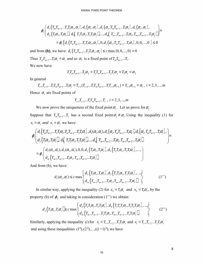
8
( ) ( ) ( ) ( )( ) ( ) ( )
1 1 2 1 1 1 1 1 1 1 1 1 1 1 1 1 11
2 1 1 1 1 3 2 1 1 2 1 1 1 2 1 1 1 2 1 1
... , , , , , ... , , ,
, , d , ,..., ... , ...m m m m
m m m m m
d T T T T d d T T T d
d T T T T T T d T T T T T T
α α α α α α α αϕ
α α α α α α− −
− − − −
=
( ) ( )( )1 1 1 2 1 1 1 1 1 1 1 1... , ,0, , ... ,0,0,...,0 0m m m md T T T T d T T Tϕ α α α α− −= ≤
and from (b), we have: ( )1 1 2 1 1 1... , max0,0,...,0 0m md T T T T cα α− ≤ =
Thus 1 1 1 1...m mT T Tα α− = and so 1α is a fixed point of 1 1...m mT T T− .
We now have
1 1 2 2 1 1 2 1 1 1 1 2... ...m m m mTT T T TTT T T Tα α α α− −= = =
In general
1 2 1 1 1 2 1 1 1 1 1 1... ... ( ... ... )i i m m i i i i m m i i i i i iT T TT T T T T TT T TT Tα α α α− − − − − − − − − −= = = , 2,3,...,i m=
Hence iα are fixed points of
1 2 1 1... ...i i m m iT T TT T T− − − , 2,3,...,i m=
We now prove the uniqueness of the fixed point iα . Let us prove for 1α .
Suppose that 1 1...m mT T T− has a second fixed point '1 1α α≠ .Using the inequality (1) for
' '1 1 1 1x and xα α= = we have:
( ) ( ) ( )( ) ( ) ( )
' ' ' '1 1 2 1 1 1 2 1 1 1 1 1 1 1 1 1 1 1 1 1 1 1
1 ' ' '2 1 1 1 1 3 2 1 1 2 1 1 1 2 1 1 1 2 1 1
... , ... , ( , ), , ... , , ... ,
, , d , ,..., ... , ...
m m m m m m m m
m m m m m
d T T TT T T TT d d T T T d T T T
d T T TT TT d T T T T T T
α α α α α α α αϕ
α α α α α α− − − −
− − − −
=
( ) ( )
( )' ' ' '
1 1 1 1 1 1 2 1 1 1 1 3 2 1 1 2 1 1
1 '1 2 1 1 1 2 1 1
( , ), ( , ),0,0, , ,d , ,...,
... , ...m m m m m
d d d T T T T TT
d T T T T T T
α α α α α α α αϕ
α α− − − −
=
And from (b), we have:
( ) ( )( )
' '2 1 1 1 1 3 2 1 1 2 1 1'
1 1 1 '1 2 1 1 1 2 1 1
, ,d , ,...,( , ) max
... , ...m m m m m
d T T T T TTd c
d T T T T T T
α α α αα α
α α− − − −
≤
(1’’)
In similar way, applying the inequality (2) for ' '2 1 1 2 1 1andx T x Tα α= = , by the
property (b) of 2ϕ and taking in consideration (1’’) we obtain:
( ) ( ) ( )( )
' '3 2 1 1 2 1 1 4 3 2 1 1 3 2 1 1'
2 1 1 1 1 '1 2 2 1 1 1 2 2 1 1
, , , ,...,, max
... , ... ,m m m m m
d T T T T d T T T T T Td T T c
d T T TT T T T T
α α α αα α
α α− − − −
≤
(2’’)
Similarly, applying the inequality ( )i for 1 2 2 1 1...i i ix T T T Tα− −= and ' '1 2 2 1 1...i i ix T T T Tα− −=
and using these inequalities (1''), (2 ''),..., (( 1) ''),i − we have
KIKINA: FIXED POINT THEOREM
76
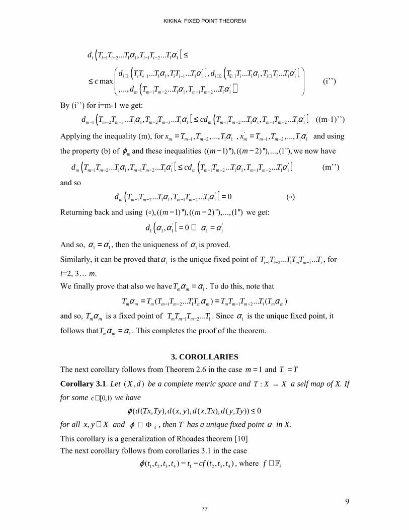
9
( )'1 2 1 1 1 2 1 1... , ...i i i i id T T T T T Tα α− − − − ≤
( ) ( )
( )' '
1 1 1 1 1 1 1 2 1 1 1 1 1 1
'1 2 1 1 1 2 1
... , ... , ... , ...max
,..., ... , ...
i i i i i i i i i i
m m m m m i
d TT T TT T d T T T T T Tc
d T T T T T T
α α α α
α α+ − − + + +
− − − −
≤
(i’’)
By (i’’) for i=m-1 we get:
( ) ( )' '1 2 3 1 1 2 3 1 1 1 2 1 1 1 2 1 1... , ... ... , ...m m m m m m m m m md T T T T T T cd T T T T T Tα α α α− − − − − − − − −≤ ((m-1)’’)
Applying the inequality (m), for 1 2 1 1, ,...,m m mx T T Tα− −= , ' '1 2 1 1, ,...,m m mx T T Tα− −= and using
the property (b) of mϕ and these inequalities (( 1) ''), (( 2) ''),..., (1''),m m− − we now have
( ) ( )' '1 2 1 1 1 2 1 1 1 2 1 1 1 2 1 1... , ... ... , ...m m m m m m m m m md T T T T T T cd T T T T T Tα α α α− − − − − − − −≤ (m’’)
and so
( )'1 2 1 1 1 2 1 1... , ... 0m m m m md T T T T T Tα α− − − − = ( )
Returning back and using ( ), (( 1) ''), (( 2) ''),..., (1'')m m− − we get:
( )' '1 1 1 1 1, 0d α α α α= ⇔ =
And so, '1 1α α= , then the uniqueness of 1α is proved.
Similarly, it can be proved that iα is the unique fixed point of 1 2 1 1... ...i i m m iT T TT T T− − − , for
i=2, 3… m. We finally prove that also we have 1m mT α α= . To do this, note that
1 2 1 1 2 1( ... ) ... ( )m m m m m m m m m m m mT T T T TT T T T T Tα α α− − − −= =
and so, m mT α is a fixed point of 1 2 1...m m mT T T T− − . Since 1α is the unique fixed point, it
follows that 1m mT α α= . This completes the proof of the theorem.
3. COROLLARIES
The next corollary follows from Theorem 2.6 in the case 1m= and 1T T=
Corollary 3.1. Let ( , )X d be a complete metric space and XXT →: a self map of X. If
for some [0,1)c∈ we have
( ( , ), ( , ), ( , ), ( , )) 0d Tx Ty d x y d x Tx d y Tyϕ ≤
for all ,x y X∈ and 4ϕ ∈ Φ , then T has a unique fixed point α in X.
This corollary is a generalization of Rhoades theorem [10] The next corollary follows from corollaries 3.1 in the case
1 2 3 4 1 2 3 4( , , , ) = ( , , )t t t t t cf t t tϕ − , where 3f ∈F
KIKINA: FIXED POINT THEOREM
77
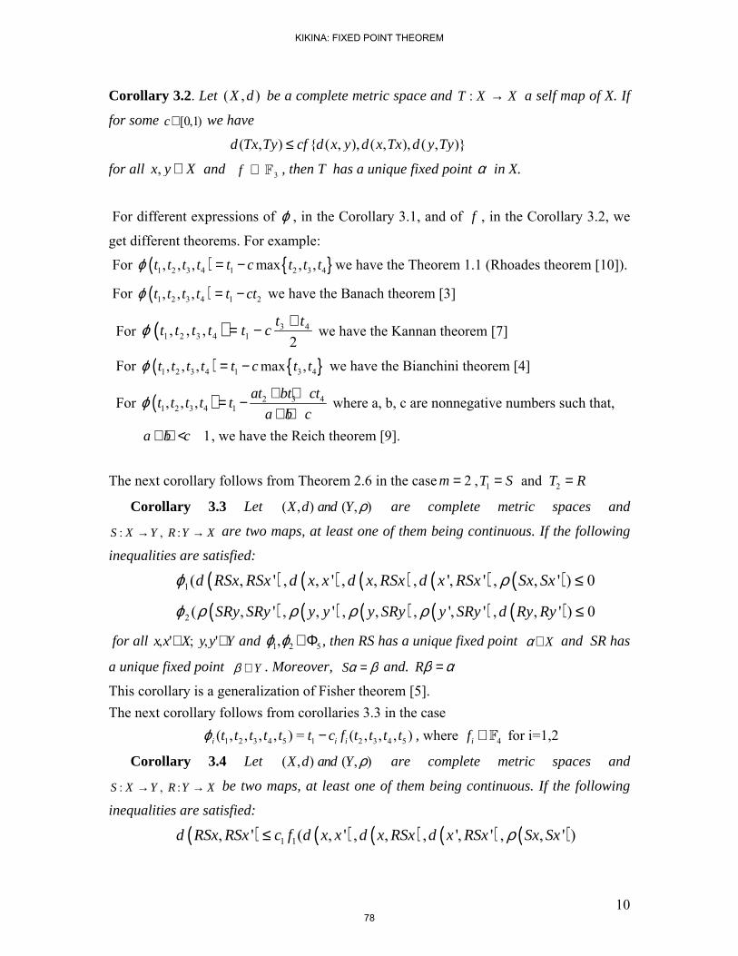
10
Corollary 3.2. Let ( , )X d be a complete metric space and XXT →: a self map of X. If
for some [0,1)c∈ we have
( , ) ( , ), ( , ), ( , )d Tx Ty cf d x y d x Tx d y Ty≤
for all ,x y X∈ and 3f ∈ F , then T has a unique fixed point α in X.
For different expressions of ϕ , in the Corollary 3.1, and of f , in the Corollary 3.2, we
get different theorems. For example:
For ( ) 1 2 3 4 1 2 3 4, , , max , ,t t t t t c t t tϕ = − we have the Theorem 1.1 (Rhoades theorem [10]).
For ( )1 2 3 4 1 2, , ,t t t t t ctϕ = − we have the Banach theorem [3]
For ( ) 3 41 2 3 4 1, , ,
2t t
t t t t t cϕ += − we have the Kannan theorem [7]
For ( ) 1 2 3 4 1 3 4, , , max ,t t t t t c t tϕ = − we have the Bianchini theorem [4]
For ( ) 2 3 41 2 3 4 1, , , at bt ctt t t t t
a b cϕ + += −
+ + where a, b, c are nonnegative numbers such that,
1a b c+ + < , we have the Reich theorem [9]. The next corollary follows from Theorem 2.6 in the case 2m= , 1 2andT S T R= =
Corollary 3.3 Let ( , ) ( , )X d and Yρ are complete metric spaces and
XYRYXS →→ : , : are two maps, at least one of them being continuous. If the following
inequalities are satisfied:
( ) ( ) ( ) ( ) ( )1( , ' , , ' , , , ', ' , , ' ) 0d RSx RSx d x x d x RSx d x RSx Sx Sxϕ ρ ≤
( ) ( ) ( ) ( ) ( )2 ( , ' , , ' , , , ', ' , , ' ) 0SRy SRy y y y SRy y SRy d Ry Ryϕ ρ ρ ρ ρ ≤
for all , ' ; , 'x x X y y Y∈ ∈ and 1 2 5,ϕ ϕ ∈Φ , then RS has a unique fixed point X∈α and SR has
a unique fixed point Y∈β . Moreover, βα =S and. αβ =R
This corollary is a generalization of Fisher theorem [5]. The next corollary follows from corollaries 3.3 in the case
1 2 3 4 5 1 2 3 4 5( , , , , ) = ( , , , )i i it t t t t t c f t t t tϕ − , where 4if ∈F for i=1,2
Corollary 3.4 Let ( , ) ( , )X d and Yρ are complete metric spaces and
XYRYXS →→ : , : be two maps, at least one of them being continuous. If the following
inequalities are satisfied:
( ) ( ) ( ) ( ) ( )1 1, ' ( , ' , , , ', ' , , ' )d RSx RSx c f d x x d x RSx d x RSx Sx Sxρ≤
KIKINA: FIXED POINT THEOREM
78
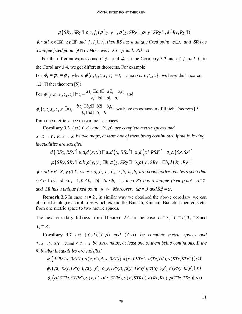
11
( ) ( ) ( ) ( ) ( )2 2, ' ( , ' , , , ', ' , , ' )SRy SRy c f y y y SRy y SRy d Ry Ryρ ρ ρ ρ≤
for all , ' ; , 'x x X y y Y∈ ∈ and 1 2 4,f f ∈F , then RS has a unique fixed point X∈α and SR has
a unique fixed point Y∈β . Moreover, βα =S and. αβ =R
For the different expressions of 1ϕ and 2ϕ in the Corollary 3.3 and of 1 2f and f in
the Corollary 3.4, we get different theorems. For example:
For 1 2ϕ ϕ ϕ= = , where ( ) 1 2 3 4 5 1 2 3 4 5, , , , max , , ,t t t t t t c t t t tϕ = − , we have the Theorem
1.2 (Fisher theorem [5]).
For ( ) 1 2 2 3 3 4 4 51 1 2 3 4 5 1
1 2 3 4
, , , , a t a t a t a tt t t t t t
a a a aϕ + + += −
+ + + and
( ) 1 2 2 3 3 4 4 52 1 2 3 4 5 1
1 2 3 4
, , , , bt b t b t b tt t t t t t
b b b bϕ + + += −
+ + +, we have an extension of Reich Theorem [9]
from one metric space to two metric spaces. Corollary 3.5. Let( , ) ( , )X d and Yρ are complete metric spaces and
XYRYXS →→ : , : be two maps, at least one of them being continuous. If the following
inequalities are satisfied:
( ) ( ) ( ) ( )1 2 3 4, ' ( , ) , ', ' , 'd RSx RSx a d x x a d x RSx a d x RSx a Sx Sxρ′≤ + + +
( ) ( ) ( ) ( )1 2 3 4, ' ( , ) , ', ' , 'SRy SRy b y y b y SRy b y SRy b d Ry Ryρ ρ ρ ρ′≤ + + +
for all , ' ; , 'x x X y y Y∈ ∈ , where 1 2 3 4, , ,a a a a , 1 2 3 4, , ,b b b b are nonnegative numbers such that
1 2 3 40 1a a a a≤ + + + < , 1 2 3 40 1b b b b≤ + + + < , then RS has a unique fixed point X∈α
and SR has a unique fixed point Y∈β . Moreover, βα =S and αβ =R .
Remark 3.6 In case 2m= , in similar way we obtained the above corollary, we can obtained analogues corollaries which extend the Banach, Kannan, Bianchin theorems etc. from one metric space to two metric spaces.
The next corollary follows from Theorem 2.6 in the case 3m= , 1 2,T T T S= = and
3T R= :
Corollary 3.7 Let ( , ), ( , )X d Y ρ and ( , )Z σ be complete metric spaces and
: , S:Y Z and :T X Y R Z X→ → → be three maps, at least one of them being continuous. If the
following inequalities are satisfied
( )1 ( , ), ( , ), ( , ), ( , ), ( , ), ( , ) 0d RSTx RSTx d x x d x RSTx d x RSTx Tx Tx STx STxϕ ρ σ′ ′ ′ ′ ′ ′ ≤
( )2 ( , ), ( , ), ( , ), ( , ), ( , ), ( , ) 0TRSy TRSy y y y TRSy y TRSy Sy Sy d RSy RSyϕ ρ ρ ρ ρ σ′ ′ ′ ′ ′ ′ ≤
( )3 ( , ), ( , ), ( , ), ( , ), ( , ), ( , ) 0STRz STRz z z z STRz z STRz d Rz Rz TRz TRzϕ σ σ σ σ ρ′ ′ ′ ′ ′ ′ ≤
KIKINA: FIXED POINT THEOREM
79
12
for all , ; , ; ,x x X y y Y z z Z′ ′ ′∈ ∈ ∈ and 1 2 3 6, ,ϕ ϕ ϕ ∈Φ , then RST has a unique fixed point
u in X , TRS has a unique fixed point v in Y and STR has a unique fixed point w in Z . Further, = , =Tu v Sv w and Rw u= . This corollary is a generalization of Jain et all theorem [6].
In the special case for ϕϕϕϕ === 321 where ( ) 1 2 3 4 5 6 1 2 3 4 5 6, , , , , max , , , ,t t t t t t t c t t t t tϕ = − ,
we have the theorem 1.2 (Jain et all theorem [6]). Remark 3.8 From the corollary 3.6 we can obtain other propositions determined by the form of implicit relations 1ϕ , 2ϕ and 3ϕ . For example the corollary which extended the theorem of Reich [6], from one metric space to three metric spaces (in similar way as above we extended to two metric spaces), etc. At last, we would like to emphasize the fact that all the above corollaries does not hold only for 1, 2 and 3 metric spaces, but also for an arbitrary number of metric spaces.
REFERENCES
[1] A. Aliouche and B. Fisher. Fixed point theorems for mappings satisfying implicit relation on two complete and compact metric spaces, Applied Mathematics and
Mechanics, 7 ( 9), (2006), 1217-1222. [2] A. Aliouche and B. Fisher, A related fixed point theorem for two pairs of mappings on
two complete metric spaces. Hacettepe Journal of Mathematics and statistics. V.34 (2005), 39-45.
[3] S. Banach. Theorie des operations lineaires Manograie, Mathematyezne (Warsaw, Poland), 1932.
[4] R. M. T. Bianchini, Su un problema di S.Reich riguardante la teoria dei punti fissi, Boll. Un. Mat. Ital.5 ( 1972) 103-108.
[5] B. Fisher. Related fixed points on two metric spaces. Math. Sem. Notes, Kobe univ., 10, 17 -26, 1982.
[6] R. K. Jain, H. K. Sahu, and B. Fisher. Related fixed points theorems for three metric spaces, Novi Sad. I. Math, Vol 26,No.1, 11-17, 1996.
[7] R. Kannan, Some results on fixed points II, Amer. Math. Monthly 76 (1969), 405-408.
[8] V. Popa, On some fixed point theorems for mappings satisfying a new type of implicit relation, Mathematica Moravica, (7), pp. 61-66, 2003.
[9] S. Reich, Some remarks concerning contraction mappings, Canad. Math. Bull. 14(1971) 121-124.
[10] B. E. Rhoades, A comparison of various definitions of contractive mappings. Trans. Amer. Math. soc. 226, (1977), 256-290.
[11] M. Telci, Fixed points on two complete and compact metric spaces, Applied Mathematics and Mechanics, 22 (5) , (2001), 564-568.
KIKINA: FIXED POINT THEOREM
80
Direct and converse theorems for generalized Bernsteinpolynomials based on the qintegers
·Ibrahim Büyükyaz¬c¬Department of Mathematics, Gazi University, Çubuk - Ankara, Turkey
e-mail: [email protected]
Abstract
In this paper, we discuss the convergence properties of a new generalization of qBernstein polynomials. The uniform convergence is established, and estimates for therate of convergence are provided. We also prove that if the rate of convergence forthese operators is C=[n] qn , then f 2 Lip( ; [0; 1]), for some positive constant C andexponent 0 < < 1.
Keywords: q Bernstein polynomials, rate of convergence, inverse theorem.
2000 Mathematics Subject Classication: 41A10, 41A25, 41A36.
1 Introduction and denitions
In some branches of mathematics (for example, approximation theory, probability theory,number theory, the solution of integral and di¤erential equations), Bernstein polynomialshave important applications. The reasons for these applications are the simple structureand important properties of the Bernstein polynomials (for example, shape preserving,reproducing linear functions, degree reducing on the set of polynomials, interpolating f atboth end points of [0; 1]). The nth Bernstein polynomial for a given function f on [0; 1] isdened as
Bn(f ;x) =nXk=0
f
k
n
Pk;n(x) (1)
where Pk;n(x) =
n
k
xk(1 x)nk; 0 x 1; n = 1; 2; 3; : : :
If f 2 C[0; 1], then the sequence fBn(f ;x)g converges uniformly to f(x) on [0; 1].In [5], J. D. Cao introduced the following generalized Bernstein polynomials (which we
call the Cao polynomials): for f 2 C[0; 1], the Cao polynomials of f are
Cn;sn(f ;x) =1
sn
nXk=0
sn1Xi=0
f(k + i
n+ sn 1)Pk;n(x); 0 x 1; n = 1; 2; 3; : : : (2)
where fsng is a sequence of natural numbers with the properties limn!1
snn= 0 and sn 1.
When sn = 1, we recover the Bernstein polynomials.Before introducing the new operators based on q integers, we recall the following de-
nitions of the q calculus (quantum calculus). Given a value of q > 0 and any nonnegativeinteger n, we dene the q integer [n]q as
[n]q =
((1 qn)=(1 q) if q 6= 1n if q = 1
1
81
JOURNAL OF APPLIED FUNCTIONAL ANALYSIS, VOL.7, NO’S 1-2,81-91,COPYRIGHT 2012 EUDOXUS PRESS,LLC
and the q factorial [n]q! as
[n]q! =
([n]q[n 1]q [1]q if n 11 if n = 0
:
For integers n and k, with 0 k n, the q binomial coe¢ cients are then dened asfollows (see [9]):
nk
q
=[n]q!
[k]q![n k]q!:
Due to the intensive development of the q calculus, generalizations of Bernstein poly-nomials based on the q integers have emerged. In [16], G. M. Phillips proposed theq Bernstein polynomials (which we also call the Phillips polynomials): for each positiveinteger n, and f 2 C[0; 1], the q Bernstein polynomial of f is
Bn;q(f ;x) =
nXk=0
f
[k]q[n]q
nk
q
xknk1Ys=0
(1 qsx); 0 x 1; n = 1; 2; 3; : : : (3)
where an empty product is taken to equal 1. Note that the Phillips polynomials reduce tothe Bernstein polynomials when we choose q = 1 in (3). Explicit expressions for Bn;q(tr;x)for r = 0; 1; 2 can be obtained by direct calculation, giving
Bn;q(1;x) = 1
Bn;q(t;x) = x (4)
Bn;q(t2;x) = x2 +
x(1 x)[n]q
:
In recent years, the q Bernstein polynomials and some generalizations have been stud-ied by several researchers because of their potential applications in approximation theoryand numerical analysis, and some features of the Bernstein polynomials are inherited bythe q Bernstein polynomials, especially for 0 < q < 1 (see [4], [10]-[20]).
In this paper, as Phillips has done for the Bernstein polynomials, we consider similarmodication of the Cao polynomials:
Bqn;n(f ;x) =1
[n]
nXk=0
[n]1Xi=0
f([k]q + i
[n]q + n 1)Pk;n;q(x); (5)
where Pk;n;q(x) =
nk
q
xknk1Ys=0
(1 qsx); 0 x 1; n = 1; 2; 3; : : :
where n is a positive real number and [n], as usual, denotes the greatest integer lessthan n. There should be no confusion between the two notations [n] and [n]q. Whenn = 1; we recover the Phillips polynomials; when q = 1 and n = sn we recover the Caopolynomials.
Note that throughout the paper, we always assume that fqng is a sequence of realnumbers such that 0 < qn < 1 for all n and lim
n!1qn = 1, and where fng is a sequence of
positive real numbers with the properties limn!1
n[n]qn
= 0 and [n] 1:The outline of this paper is as follows: in Section 2, we give the convergence properties
of the polynomials (5). Section 3 deals with the rate of convergence, using di¤erentmethods. Finally, we prove an inverse theorem for the polynomials (5).
Now, we give the following basic denitions:
2
BUYUKYAZICI: q-BERNSTEIN POLYNOMIALS
82
Denition 1.1. The q derivative of a function f with respect to x is
Dq (f(x)) =f(qx) f(x)qx x ;
and this is also known as the Jackson derivative.
The q derivative product ruleis Dq (f(x)g(x)) = Dq (f(x)) g(qx) + f(x)Dq (g(x)).Note also that Dq (xn) = [n]qxn1.
Denition 1.2. The q integral of a function f isZ b
af(x)dqx = (1 q)b
1Xm=0
qmf(bqm) (1 q)a1Xm=0
qmf(aqm):
Note that as q ! 1, the q derivative and the q integral approach the usual derivativeand the Riemann integral, respectively.
Denition 1.3. For f 2 C[0; 1] and > 0, the usual modulus of continuity is dened by
!(f ; ) = supjxyjx;y2[0;1]
jf(x) f(y)j :
It is known that lim!0 !(f ; ) = 0 and, for any > 0, !(f ;) (1 + )!(f ; ).
Denition 1.4. For > 0 and C2[0; 1] = fg 2 C[0; 1] : g0; g00 2 C[0; 1]g, Peetres Kfunctional is dened as
K(f ; ) = infg2C2[0;1]
nkf gkC[0;1] + kgkC2[0;1]
owhere k:kC2[0;1] is the uniform norm on C2[0; 1]; dened by
kgkC2[0;1] = g0
C[0;1]+ g00
C[0;1]:
2 Approximation properties of Bqnn;nFrom the denition (5) of Bqnn;n(f ;x) and the rst equation in (4), we have
Bqnn;n(1;x) = 1: (6)
To construct our approximation theorem for the sequence fBqnn;ng, we need the followinglemma.
Lemma 2.1. If the operator Bqnn;n is dened by (5), then
Bqnn;n(t;x) =[n]qn
[n]qn + n 1x+
[n] 12 ([n]qn + n 1)
; (7)
Bqnn;n(t2;x) =
[n]2qn [n]qn([n]qn + n 1)2
x2 +[n] [n]qn
([n]qn + n 1)2x+
([n] 1)(2 [n] 1)6([n]qn + n 1)2
:(8)
Proof. Let us consider the case when f is the function t 7! t; then
Bqnn;n(t;x) =1
[n]
nXk=0
[n]1Xi=0
[k]qn + i
[n]qn + n 1Pk;n;qn(x)
=1
[n]
1
[n]qn + n 1
([n] [n]qn
nXk=0
[k]qn[n]qn
Pk;n;qn(x)
+1
2([n] 1) [n]
nXk=0
Pk;n;qn(x)
):
3
BUYUKYAZICI: q-BERNSTEIN POLYNOMIALS
83
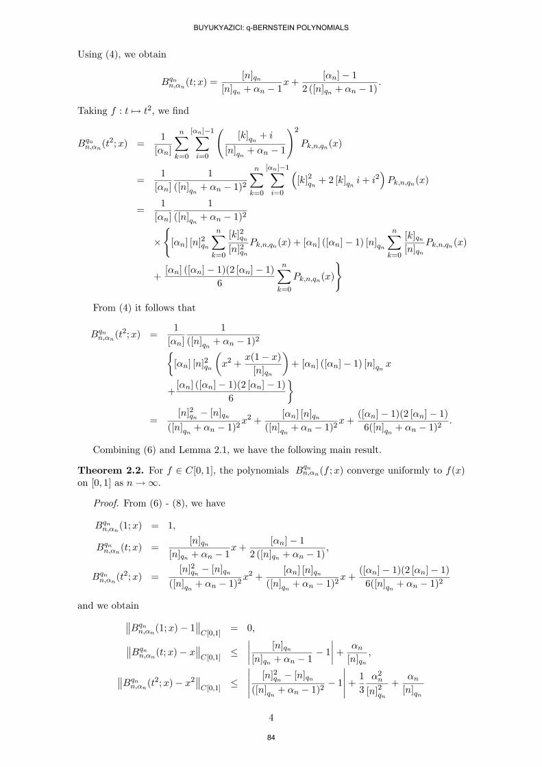
Using (4), we obtain
Bqnn;n(t;x) =[n]qn
[n]qn + n 1x+
[n] 12 ([n]qn + n 1)
:
Taking f : t 7! t2, we nd
Bqnn;n(t2;x) =
1
[n]
nXk=0
[n]1Xi=0
[k]qn + i
[n]qn + n 1
!2Pk;n;qn(x)
=1
[n]
1
([n]qn + n 1)2nXk=0
[n]1Xi=0
[k]2qn + 2 [k]qn i+ i
2Pk;n;qn(x)
=1
[n]
1
([n]qn + n 1)2
([n] [n]
2qn
nXk=0
[k]2qn[n]2qn
Pk;n;qn(x) + [n] ([n] 1) [n]qnnXk=0
[k]qn[n]qn
Pk;n;qn(x)
+[n] ([n] 1)(2 [n] 1)
6
nXk=0
Pk;n;qn(x)
)
From (4) it follows that
Bqnn;n(t2;x) =
1
[n]
1
([n]qn + n 1)2[n] [n]
2qn
x2 +
x(1 x)[n]qn
+ [n] ([n] 1) [n]qn x
+[n] ([n] 1)(2 [n] 1)
6
=
[n]2qn [n]qn([n]qn + n 1)2
x2 +[n] [n]qn
([n]qn + n 1)2x+
([n] 1)(2 [n] 1)6([n]qn + n 1)2
:
Combining (6) and Lemma 2.1, we have the following main result.
Theorem 2.2. For f 2 C[0; 1], the polynomials Bqnn;n(f ;x) converge uniformly to f(x)on [0; 1] as n!1.
Proof. From (6) - (8), we have
Bqnn;n(1;x) = 1;
Bqnn;n(t;x) =[n]qn
[n]qn + n 1x+
[n] 12 ([n]qn + n 1)
;
Bqnn;n(t2;x) =
[n]2qn [n]qn([n]qn + n 1)2
x2 +[n] [n]qn
([n]qn + n 1)2x+
([n] 1)(2 [n] 1)6([n]qn + n 1)2
and we obtain Bqnn;n(1;x) 1 C[0;1] = 0; Bqnn;n(t;x) x C[0;1] [n]qn[n]qn + n 1
1+ n
[n]qn;
Bqnn;n(t2;x) x2 C[0;1] [n]2qn [n]qn([n]qn + n 1)2
1+ 13 2n
[n]2qn+
n[n]qn
4
BUYUKYAZICI: q-BERNSTEIN POLYNOMIALS
84

from condition limn!1
n[n]qn
= 0; we get
limn!1
Bqnn;n(tr;x) xr C[0;1] = 0; r = 0; 1; 2:
The proof of uniform convergence is then completed by applying the well-known Korovkintheorem (see [1]).
3 Rate of convergence
Theorem 3.1. For any f 2 C[0; 1],
Bqnn;n(f ;x) f(x) 2!0@f ;
q42n + [n]qn
[n]qn
1Awhere !(f ; ) is the modulus of continuity as given in Denition 1.3.
Proof. Using the relation 1[n]
Pnk=0
P[n]1i=0 f(x)Pk;n;qn(x) = f(x), express the di¤er-
ence between Bqnn;n(f ;x) and f as
Bqnn;n(f ;x) f(x) =1
[n]
nXk=0
[n]1Xi=0
"f(
[k]qn + i
[n]qn + n 1) f(x)
#Pk;n;qn(x)
and so
Bqnn;n(f ;x) f(x) 1
[n]
nXk=0
[n]1Xi=0
f( [k]qn + i
[n]qn + n 1) f(x)
Pk;n;qn(x) (9)
Letting y =[k]qn + i
[n]qn + n 1and jy xj = , we have jf(y) f(x)j !(f ;) (1 +
)!(f ; ). Thus jf(y) f(x)j 1 + jyxj
!(f ; ), and hence, by (6)
Bqnn;n(f ;x) f(x) 1
[n]!(f ; )
nXk=0
[n]1Xi=0
0B@1 + [k]qn+i
[n]qn+n1 x
1CAPk;n;qn(x) !(f ; )
8><>:1 + 124 1
[n]
nXk=0
[n]1Xi=0
[k]qn + i
[n]qn + n 1 x!2Pk;n;qn(x)
351=29>=>;
where we have invoked the Cauchy-Schwartz inequality. Expanding the squared term andmaking use of (6), (7) and (8), we obtain
Bqnn;n(f ;x) f(x) !(f ; )
1 +
1
"
[n]2qn [n]qn([n]qn + n 1)2
x2 +[n] [n]qn
([n]qn + n 1)2x+
([n] 1)(2 [n] 1)6([n]qn + n 1)2
2x
[n]qn[n]qn + n 1
x+[n] 1
2 ([n]qn + n 1)
+ x2
1=2): (10)
5
BUYUKYAZICI: q-BERNSTEIN POLYNOMIALS
85

Now, since 0 x 1 and 1 [n] n, by choosing =
p42n + [n]qn[n]qn
in (10), we
deduce
1
[n]
nXk=0
[n]1Xi=0
[k]qn + i
[n]qn + n 1 x!2Pk;n;qn(x)
=
[n]2qn [n]qn
([n]qn + n 1)2 2[n]qn[n]qn + n 1
+ 1
!x2
+
[n] [n]qn
([n]qn + n 1)2 [n] 1[n]qn + n 1
!x+
([n] 1)(2 [n] 1)6([n]qn + n 1)2
=(n 1)2 [n]qn([n]qn + n 1)2
x2 +[n] + [n]qn + n [n]n 1
([n]qn + n 1)2x+
([n] 1)(2 [n] 1)6([n]qn + n 1)2
2n([n]qn + n 1)2
x2 +[n] + [n]qn + n([n]qn + n 1)2
x+[n]
2
3([n]qn + n 1)2
2n([n]qn + n 1)2
+2n + [n]qn
([n]qn + n 1)2+
2n3([n]qn + n 1)2
42n + [n]qn
[n]2qn= 2 (11)
so that Bqnn;n(f ;x) f(x) 2 ! f ;
p42n + [n]qn[n]qn
!as claimed.
Theorem 3.2. If f is Hölder continuous on [0; 1] with exponent 2 (0; 1], denotedf 2 LipM ( ; [0; 1]) with 0 < 1, thenBqnn;n(f ;x) f(x) M
p42n + [n]qn[n]qn
! Proof. From (9) we have
Bqnn;n(f ;x) f(x) 1
[n]
nXk=0
[n]1Xi=0
f( [k]qn + i
[n]qn + n 1) f(x)
Pk;n;qn(x) M
[n]
nXk=0
[n]1Xi=0
[k]qn + i
[n]qn + n 1 x
Pk;n;qn(x)
by the Hölder condition. Application of Hölders inequality gives
Bqnn;n(f ;x) f(x) M
[n]
8<:nXk=0
[n] 1Xi=0
[k]qn + i
[n]qn + n 1 x2
Pk;n;qn(x)
9=; 2 ( nX
k=0
Pk;n;qn(x)
) 2 2
= M
8<:nXk=0
1
[n]2
[n]1Xi=0
[k]qn + i
[n]qn + n 1 x!2Pk;n;qn(x)
9=; 2
M
8<:nXk=0
1
[n]
[n]1Xi=0
[k]qn + i
[n]qn + n 1 x!2Pk;n;qn(x)
9=; 2
M
p42n + [n]qn[n]qn
!
6
BUYUKYAZICI: q-BERNSTEIN POLYNOMIALS
86
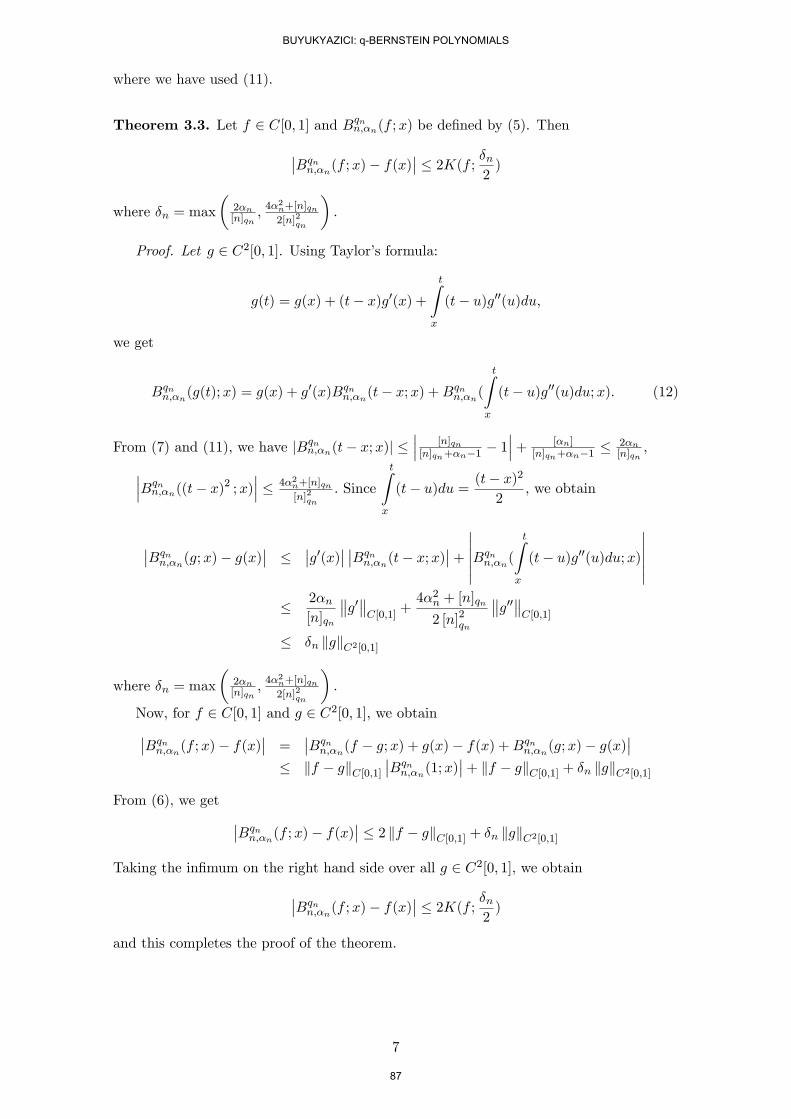
where we have used (11).
Theorem 3.3. Let f 2 C[0; 1] and Bqnn;n(f ;x) be dened by (5). ThenBqnn;n(f ;x) f(x) 2K(f ; n2 )where n = max
2n[n]qn
;42n+[n]qn2[n]2qn
:
Proof. Let g 2 C2[0; 1]. Using Taylors formula:
g(t) = g(x) + (t x)g0(x) +tZx
(t u)g00(u)du;
we get
Bqnn;n(g(t);x) = g(x) + g0(x)Bqnn;n(t x;x) +B
qnn;n(
tZx
(t u)g00(u)du;x): (12)
From (7) and (11), we have jBqnn;n(t x;x)j [n]qn[n]qn+n1
1+ [n]
[n]qn+n1 2n
[n]qn;Bqnn;n((t x)2 ;x) 42n+[n]qn
[n]2qn: Since
tZx
(t u)du = (t x)22
; we obtain
Bqnn;n(g;x) g(x) g0(x) Bqnn;n(t x;x)+
Bqnn;n(tZx
(t u)g00(u)du;x)
2n
[n]qn
g0 C[0;1]
+42n + [n]qn
2 [n]2qn
g00 C[0;1]
n kgkC2[0;1]
where n = max2n[n]qn
;42n+[n]qn2[n]2qn
:
Now, for f 2 C[0; 1] and g 2 C2[0; 1]; we obtainBqnn;n(f ;x) f(x) =Bqnn;n(f g;x) + g(x) f(x) +Bqnn;n(g;x) g(x)
kf gkC[0;1]Bqnn;n(1;x)+ kf gkC[0;1] + n kgkC2[0;1]
From (6), we get Bqnn;n(f ;x) f(x) 2 kf gkC[0;1] + n kgkC2[0;1]Taking the inmum on the right hand side over all g 2 C2[0; 1], we obtain
Bqnn;n(f ;x) f(x) 2K(f ; n2 )and this completes the proof of the theorem.
7
BUYUKYAZICI: q-BERNSTEIN POLYNOMIALS
87
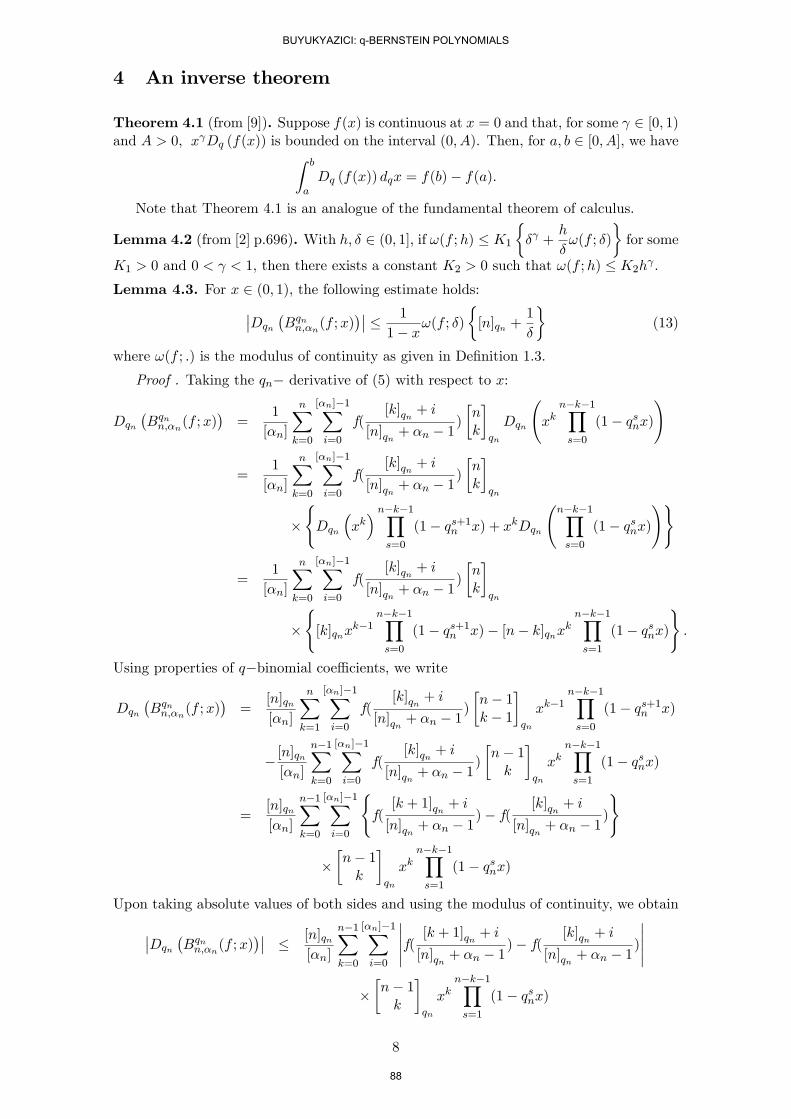
4 An inverse theorem
Theorem 4.1 (from [9]). Suppose f(x) is continuous at x = 0 and that, for some 2 [0; 1)and A > 0, x Dq (f(x)) is bounded on the interval (0; A). Then, for a; b 2 [0; A], we haveZ b
aDq (f(x)) dqx = f(b) f(a):
Note that Theorem 4.1 is an analogue of the fundamental theorem of calculus.
Lemma 4.2 (from [2] p.696). With h; 2 (0; 1], if !(f ;h) K1 +
h
!(f ; )
for some
K1 > 0 and 0 < < 1, then there exists a constant K2 > 0 such that !(f ;h) K2h .Lemma 4.3. For x 2 (0; 1), the following estimate holds:Dqn Bqnn;n(f ;x) 1
1 x!(f ; )[n]qn +
1
(13)
where !(f ; :) is the modulus of continuity as given in Denition 1.3.
Proof . Taking the qn derivative of (5) with respect to x:
DqnBqnn;n(f ;x)
=
1
[n]
nXk=0
[n]1Xi=0
f([k]qn + i
[n]qn + n 1)
nk
qn
Dqn
xk
nk1Ys=0
(1 qsnx)!
=1
[n]
nXk=0
[n]1Xi=0
f([k]qn + i
[n]qn + n 1)
nk
qn
(Dqn
xk nk1Y
s=0
(1 qs+1n x) + xkDqn
nk1Ys=0
(1 qsnx)!)
=1
[n]
nXk=0
[n]1Xi=0
f([k]qn + i
[n]qn + n 1)
nk
qn
([k]qnx
k1nk1Ys=0
(1 qs+1n x) [n k]qnxknk1Ys=1
(1 qsnx)):
Using properties of qbinomial coe¢ cients, we write
DqnBqnn;n(f ;x)
=
[n]qn[n]
nXk=1
[n]1Xi=0
f([k]qn + i
[n]qn + n 1)
n 1k 1
qn
xk1nk1Ys=0
(1 qs+1n x)
[n]qn[n]
n1Xk=0
[n]1Xi=0
f([k]qn + i
[n]qn + n 1)
n 1k
qn
xknk1Ys=1
(1 qsnx)
=[n]qn[n]
n1Xk=0
[n]1Xi=0
(f([k + 1]qn + i
[n]qn + n 1) f(
[k]qn + i
[n]qn + n 1)
)
n 1k
qn
xknk1Ys=1
(1 qsnx)
Upon taking absolute values of both sides and using the modulus of continuity, we obtain
Dqn Bqnn;n(f ;x) [n]qn[n]
n1Xk=0
[n]1Xi=0
f( [k + 1]qn + i[n]qn + n 1) f(
[k]qn + i
[n]qn + n 1)
n 1k
qn
xknk1Ys=1
(1 qsnx)
8
BUYUKYAZICI: q-BERNSTEIN POLYNOMIALS
88
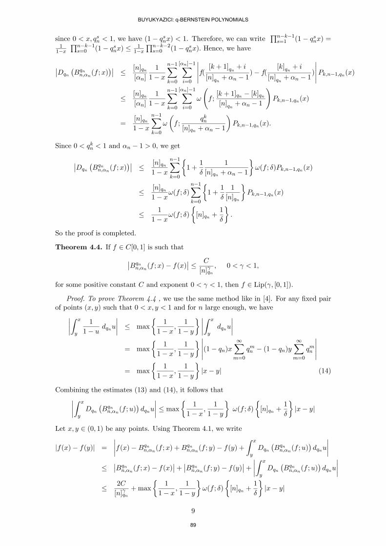
since 0 < x; qsn < 1; we have (1 qsnx) < 1. Therefore, we can writeQnk1s=1 (1 qsnx) =
11x
Qnk1s=0 (1 qsnx) 1
1xQnk2s=0 (1 qsnx): Hence, we have
Dqn Bqnn;n(f ;x) [n]qn[n]
1
1 x
n1Xk=0
[n]1Xi=0
f( [k + 1]qn + i[n]qn + n 1) f(
[k]qn + i
[n]qn + n 1)
Pk;n1;qn(x) [n]qn
[n]
1
1 x
n1Xk=0
[n]1Xi=0
!
f ;[k + 1]qn [k]qn[n]qn + n 1
!Pk;n1;qn(x)
=[n]qn1 x
n1Xk=0
!
f ;
qkn[n]qn + n 1
Pk;n1;qn(x):
Since 0 < qkn < 1 and n 1 > 0, we get
Dqn Bqnn;n(f ;x) [n]qn1 x
n1Xk=0
1 +
1
1
[n]qn + n 1
!(f ; )Pk;n1;qn(x)
[n]qn1 x!(f ; )
n1Xk=0
1 +
1
1
[n]qn
Pk;n1;qn(x)
1
1 x!(f ; )[n]qn +
1
:
So the proof is completed.
Theorem 4.4. If f 2 C[0; 1] is such thatBqnn;n(f ;x) f(x) C
[n] qn; 0 < < 1;
for some positive constant C and exponent 0 < < 1, then f 2 Lip( ; [0; 1]).
Proof. To prove Theorem 4.4 , we use the same method like in [4]. For any xed pairof points (x; y) such that 0 < x; y < 1 and for n large enough, we haveZ x
y
1
1 u dqnu max
1
1 x;1
1 y
Z x
ydqnu
= max
1
1 x;1
1 y
(1 qn)x1Xm=0
qmn (1 qn)y1Xm=0
qmn
= max
1
1 x;1
1 y
jx yj (14)
Combining the estimates (13) and (14), it follows thatZ x
yDqn
Bqnn;n(f ;u)
dqnu
max 1
1 x;1
1 y
!(f ; )
[n]qn +
1
jx yj
Let x; y 2 (0; 1) be any points. Using Theorem 4.1, we write
jf(x) f(y)j =
f(x)Bqnn;n(f ;x) +Bqnn;n(f ; y) f(y) + Z x
yDqn
Bqnn;n(f ;u)
dqnu
Bqnn;n(f ;x) f(x)+ Bqnn;n(f ; y) f(y)+ Z x
yDqn
Bqnn;n(f ;u)
dqnu
2C
[n] qn+max
1
1 x;1
1 y
!(f ; )
[n]qn +
1
jx yj
9
BUYUKYAZICI: q-BERNSTEIN POLYNOMIALS
89
For a xed n, pick 2 (0; 1] such that 1
[n]qn 1 + qn
[n]qn. Then
1 + qn
2
, because
0 < qn < 1; and consequently
jf(x) f(y)j 2C + 3jx yj
max
1
1 x;1
1 y
!(f ; ):
Taking the maximum over all arbitrary pairs x; y 2 (0; 1) with jxyj = h 1 (x+ h; y + h 1),the last inequality gives
!(f ;h) C 0 +
h
!(f ; )
where C 0 = max f2C; 3=hg and 0 < h; 1. Lemma 4.2 then tells us that !(f ;h) C 00h for some constant C 00. The proof of Theorem 4.4 is completed.
References
[1] F. Altomare, M. Campiti, Korovkin-type Approximation Theory and its Applications,de Gruyter Studies in Mathematics, Vol.17, Walter de Gruyter & Co., Berlin-NewYork, 1994.
[2] H. Berens, G. G. Lorentz, Inverse theorems for Bernstein polynomials, Indiana Univ.Math. J., 21(8), 693708 (1972).
[3] ·I. Büyükyaz¬c¬, E. ·Ibikli, Inverse theorems for Bernstein-Chlodowsky type polynomi-als, Journal of Mathematics of Kyoto University, 46(1), 2129 (2006).
[4] ·I. Büyükyaz¬c¬, Direct and Inverse Results For Generalized q Bernstein Polynomials,Far East J. Appl. Math., 34(2),191-204 (2009) .
[5] J. D. Cao, A Generalization of the Bernstein Polynomials, J. Math. Anal. Appl., 209,140-146 (1997).
[6] R.A. DeVore, G.G. Lorentz, Constructive Approximation, Springer Verlag, Berlin,1993.
[7] C. Ding, Approximation By Generalized Bernstein Polynomials, Indian J. Pure Appl.Math., 35(6), 817-826 (2004).
[8] A. Hac¬yev, H. Hac¬saliho¼glu, Convergence of the sequences of linear positive opera-tors. Ankara University, Ankara, 1995 (in Turkish).
[9] V. Kac, P. Cheung, Quantum Calculus. Springer, New York, 2002.
[10] H. Karsli, V. Gupta, Some approximation properties of q Chlodowsky operators,Applied Mathematics and Computation, 195, 220-229 (2008).
[11] G. Nowak, Approximation properties for generalized q Bernstein polynomials, J.Math. Anal. Appl., 350, 5055 (2009).
[12] H. Oruç, G. M. Phillips, q Bernstein polynomials and Bezier curves, Journal ofComputational and Applied Mathematics, 151, 112 (2003).
[13] H. Oruç, N. Tuncer, On the Convergence and Iterates of q Bernstein Polynomials,Journal of Approximation Theory,117, 301313 (2002).
[14] S. Ostrovska, q Bernstein polynomials and their iterates, J. Approx. Theory, 123(2),232255 (2003).
10
BUYUKYAZICI: q-BERNSTEIN POLYNOMIALS
90

[15] S. Ostrovska, q Bernstein polynomials of the Cauchy kernel, Applied Mathematicsand Computation, 198, 261270 (2008).
[16] G. M. Phillips, Bernstein polynomials based on the q integers, Ann. Numer. Math.,4, 511518, (1997).
[17] G. M. Phillips, A survey of results on the q Bernstein polynomials, IMA Journal ofNumerical Analysis, 30, 277288 (2010).
[18] G.M. Phillips. Interpolation and Approximation by Polynomials, Springer-Verlag,New York, 2003.
[19] V. S. Videnskii, On some classes of q parametric positive operators, Operator TheoryAdv. Appl., 158, 213222 (2005).
[20] H. Wang, F. Meng, The rate of convergence of q Bernstein polynomials, Journal ofApproximation Theory, 136, 151 158 (2005).
11
BUYUKYAZICI: q-BERNSTEIN POLYNOMIALS
91

A NEW NON-UNIQUE FIXED POINT THEOREM
ERDAL KARAPINAR
Abstract. In this manuscript, a new non-unique fixed point theorem is proved
on usual complete metric spaces. In particular, a self-mapping T on a complete
metric space (X, d) has a non-unique fixed point if T satisfies the condition
ad(Tx, Ty)+b[d(x, Tx)+d(y, Ty)
]+c[d(y, Tx)+d(x, Ty)] ≤ sd(x, y)+rd(x, T 2x)
for all x, y ∈ X where 0 ≤ s−ca+b
< 1, a + b 6= 0, a + b + c > 0 and 0 ≤ c − r.
It is also shown that the operator T still has a fixed point if one replaces acomplete metric space (X, d) with a complete TVS-cone metric space (X, p).
1. Introduction
A certain class of maps in metric spaces with non-unique fixed points is intro-duced by Ciric ([7]). After this work, many authors (see, e.g. [11, 3, 18, 8, 19])have studied on this class of maps.
TVS-cone metric spaces are spaces with a metric that takes values in a topologicalvector space ordered by a cone [10]. If the notion ”topological vector space” isreplaced by ”Banach space” in this definition, then TVS-cone metric spaces arecalled ”Banach valued metric spaces” or ”cone metric spaces” (see [12] and also[1, 2, 4, 13, 14, 15, 16, 17]).
In this manuscript, in section 2, a new non-unique fixed point theorem is provedon complete metric space. In section 3, it is proved that this theorem stays validalso on complete TVS-cone metric spaces.
2. A Fixed Point Theorem on Usual Metric Spaces
Theorem 1. Let (X, d) be a complete metric space. Suppose there exist a, b, c, s, rand T : X → X satisfies the conditions
0 ≤ s− ca+ b
< 1, a+ b 6= 0, a+ b+ c > 0 and 0 ≤ c− r (2.1)
ad(Tx, Ty) + b[d(x, Tx) + d(y, Ty)
]+ c[d(y, Tx) + d(x, Ty)] ≤ sd(x, y) + rd(x, T 2x)
(2.2)hold for all x, y ∈ X. Then, T has at least one fixed point.
Proof. Let x0 ∈ X be arbitrary . Define a sequence xn in the following way:
xn+1 := Txn n = 0, 1, 2, ... (2.3)
When we substitute x = xn and y = xn+1 on the inequality (2.2), it implies that
ad(Txn, Txn+1) + b[d(xn, Txn) + d(xn+1, Txn+1)
]+ 4c[d(xn+1, Txn) + d(xn, Txn+1)]
≤ sd(xn, xn+1) + rd(xn, T2xn)
(2.4)
2000 Mathematics Subject Classification. 47H10,54H25,46J10, 46J15.Key words and phrases. Fixed Point Theorem, Cone Metric Spaces, TVS-Cone Metric Spaces.
1
92
JOURNAL OF APPLIED FUNCTIONAL ANALYSIS, VOL.7, NO’S 1-2,92-97,COPYRIGHT 2012 EUDOXUS PRESS,LLC
2 ERDAL KARAPINAR
for all a, b, c, s, r that satisfy (2.1). Due to (2.3), the statement (2.4) turns into
ad(xn+1, xn+2) + b[d(xn, xn+1) + d(xn+1, xn+2)
]+ c[d(xn+1, xn+1) + d(xn, xn+2)]
≤ sd(xn, xn+1) + rd(xn, xn+2).(2.5)
By a simple calculation, one can get
(a+ b)d(xn+1, xn+2) + (c− r)d(xn, xn+2) ≤ (s− b)d(xn, xn+1) (2.6)
which implies
d(xn+1, xn+2) ≤ kd(xn, xn+1) (2.7)
where k = s−ba+b . Due to (2.1), we have 0 ≤ k < 1. Taking account of (2.7), we get
inductively
d(xn, xn+1) ≤ kd(xn−1, xn) ≤ k2d(xn−2, xn−1) ≤ · · · ≤ knd(x0, x1). (2.8)
To show that xn is a Cauchy sequence, assume n > m. Then by (2.8) andtriangular inequality, one can obtain
d(xn, xm) ≤ d(xn, xn−1) + d(xn−1, xn+1) + · · ·+ d(xm−1, xm)≤ knd(x0, x1) + kn−1d(x0, x1) + · · ·+ kmd(x0, x1)
≤ km
1−kd(x0, x1).(2.9)
which concludes that xn is a Cauchy sequence.Since (X, d) is complete, the sequence xn converges to some element of X,
namely z.To show z is a fixed point of T , it is sufficient to substitute x = z and y = xn
on the inequality (2.2). Indeed,
ad(Txn, T z) + b[d(xn, Txn) + d(z, Tz)
]+ c[d(z, Txn) + d(xn, T z)]≤ sd(xn, z) + rd(xn, T
2xn)(2.10)
which is equivalent to
ad(xn+1, T z) + b[d(xn, xn+1) + d(z, Tz))
]+ c[d(z, xn+1) + d(xn+1, T z)]≤ sd(xn, z) + rd(xn, xn+2).
(2.11)Consequently, (a+ b+ c)d(Tz, z) ≤ 0 as n→∞. Thus, Tz = z as a+ b+ c > 0.
3. A Fixed Point Theorem on TVS-Cone Metric Spaces
Throughout this section, the pair (E,S) stands for a real Hausdorff locally convextopological vector space E with its generating system of semi-norms S. A non-empty subset P of E is called a cone if P + P ⊂ P , λP ⊂ P for λ ≥ 0 andP ∩ (−P ) = 0. The cone P will be assumed to be closed as well. For a givencone P , a partial ordering (denoted by ≤: or ≤P ) with respect to P can be definedas follow: x ≤ y if and only if y − x ∈ P . The notation x < y indicates that x ≤ yand x 6= y. Analogously, x << y represent that y − x ∈ intP , where intP denotesthe interior of P . Here, the continuity of the algebraic operations in a topologicalvector space and the properties of the cone imply the following relations:
intP + intP ⊆ intP and
λ(intP ) ⊆ intP (λ > 0).
93
A NEW NON-UNIQUE FIXED POINT THEOREM 3
Definition 2. (See [6], [9], [10]) For c ∈ intP , the nonlinear scalarization functionφc : E → R is defined by
φc(y) = inft ∈ R : y ∈ tc− P, for all y ∈ E.
Lemma 3. (See [6], [9], [10]) For each t ∈ R and y ∈ E, the following are satisfied:
(i) φc(y) < t⇔ y ∈ tc− intP ,(ii) if y1 ∈ y2 + P , then φc(y2) ≤ φc(y1),
(iii) φc(y1 + y2) ≤ φc(y1) + φc(y2), for all y1, y2 ∈ E.
Definition 4. Let X be a non-empty set. and E as usual a Hausdorff locally convextopological space. Suppose a vector-valued function p : X ×X → E satisfies:
(M1) 0 ≤ p(x, y) and p(x, y) = 0 if and only if x = y, for all x, y ∈ X,(M2) p(x, y) = p(y, x) for all x, y ∈ X(M3) p(x, y) ≤ p(x, z) + p(z, y), for all x, y, z ∈ X.
Then, p is called TVS-cone metric on X, and the pair (X, p) is called a TVS-conemetric space (in short, TVS-CMS).
Remark 5. In [12], the authors considered E as a real Banach space in the def-inition of TVS-CMS. Thus, a cone metric space (in short, CMS) in the sense ofHuang and Zhang [12] is a special case of TVS-CMS.
Lemma 6. (See [10]) Let (X, p) be a TVS-CMS. Then, dp : X × X → [0,∞)defined by dp = φc p is a metric.
Remark 7. Since a cone metric space (X, p) in the sense of Huang and Zhang[12], is a special case of TVS-CMS, then dp : X×X → [0,∞) defined by dp = φc dis also a metric.
Definition 8. (See [10]) Let (X, p) be a TVS-CMS, x ∈ X and xn∞n=1 a sequencein X.
(i) xn∞n=1 TVS-cone converges to x ∈ X whenever for every 0 << c ∈ E,there is a natural number M such that p(xn, x) << c for all n ≥ M and
denoted by cone− limn→∞ xn = x (or xncone→ x as n→∞),
(ii) xn∞n=1 TVS-cone Cauchy sequence in (X, p) whenever for every 0 << c ∈E, there is a natural number M such that p(xn, xm) << c for all n,m ≥M ,
(iii) (X, p) is TVS-cone complete if every sequence TVS-cone Cauchy sequencein X is a TVS-cone convergent.
Lemma 9. (See [10]) Let (X, p) be a TVS-CMS, x ∈ X and xn∞n=1 a sequencein X. Set dp = φc p. Then the following statements hold:
(i) If xn∞n=1 converges to x in TVS-CMS (X, p), then dp(xn, x) → 0 asn→∞,
(ii) If xn∞n=1 is Cauchy sequence in TVS-CMS (X, p), then xn∞n=1 is aCauchy sequence (in usual sense) in (X, dp),
(iii) If (X, p) is complete TVS-CMS, then (X, dp) is a complete metric space.
Remark 10. Note that the implications in (i) and (ii) of Lemma 9 are also con-versely true. (See e.g. [1])
94
4 ERDAL KARAPINAR
Proposition 11. (See [10]) Let (X, p) is complete TVS-CMS and T : X → Xsatisfy the contractive condition
p(Tx, Ty) ≤ kp(x, y) (3.1)
for all x, y ∈ X and 0 ≤ k < 1. Then, T has a unique fixed point in X. Moreover,for each x ∈ X, the iterative sequence Tnx∞n=1 converges to fixed point.
Definition 12. (See [5]) A subset of A of an order vector space (X, τ) via a coneP is said to be P−full if for each x, y ∈ A we have a ∈ E : x ≤ a ≤ y ⊂ A. Acone P of a topological vector space (X, τ) is said to be normal whenever τ has abase of zero consisting of P− full sets.
Theorem 13. (See [5]) (a) A cone P of a topological vector space (X, τ) is normalif and only if whenever xα and yα, α ∈ ∆ are two nets in X with 0 ≤ xα ≤ yαfor each α ∈ ∆ and yα → 0, then xα → 0.
(b) Let (X, τ) be an ordered locally convex space. A semi-norm q on X is calledmonotone if q(x) ≤ q(y) for all x, y ∈ X with 0 ≤ x ≤ y The cone of (X, τ)is normal if and only if τ is generated by a family of monotone τ− continuoussemi-norms.
In particular, if P is a cone of a real Banach space E, then it is called normal ifthere is a number K ≥ 1 such that for all x, y ∈ E: 0 ≤ x ≤ y ⇒ ‖x‖ ≤ K‖y‖. Theleast positive integer K, satisfying this inequality, is called the normal constant ofP .
The following two lemmas generalizes Lemma 1, Lemma 4 and Lemma 5 in [12].
Lemma 14. (see [2]) Let (X, p) be a cone metric space over a locally convex space(E,S), where S is the family of semi-norms defining the locally convex topology.Let xn be a sequence in E. Then
(i) xn → x in (X, p) if and only if p(xn, x)→ 0 in (E,S).(ii) xn is Cauchy in (X, p) if and only if limm,n→∞ p(xn, xm) = 0 in (E,S).
Proof. (i) Suppose xn converges to x. Let ε > 0 and q ∈ S be given, choosec >> 0 such that q(c) < ε. This is possible by taking c = εc0
2q(c0), where c0 is an
interior point of P . Then there is n0 such that p(xn, x) << c, for all n > n0. Thenby normality of the cone P we have q(p(xn, x)) ≤ q(c) < ε for all n > n0. Thismeans p(xn, x)→ 0 in (E,S). Conversely, suppose that p(xn, x)→ 0 in (E,S). Forc ∈ E with c >> 0 find δ > 0 and ρ ∈ S such that q(b) < δ implies b << c. For thisδ and this p find n0 such that q(p(xn, x)) < δ for all n > n0 and so p(xn, x) << cfor all n > n0. Therefore xn → x in (X, p).
(ii) The proof is similar to that in (i).
Lemma 15. (see [2]) Let (X, p) be a TVS-cone metric space over a normal coneof a locally convex space (E,S), where S is the family of semi-norms defining thelocally convex topology. Let xn and yn be two sequences in X and xn → x,yn → y. Then p(xn, yn)→ p(x, y) in (E,S).
Proof. Let ε > 0 and q ∈ S be given. Choose c ∈ E with c >> 0 such that q(c) <ε
6.
From xn → x and yn → y, find n0 such that for all n > n0, p(xn, x) << c andp(yn, y) << c. Then for all n > n0 we have
p(xn, yn) ≤ p(xn, x) + p(x, y) + p(y, yn) ≤ p(x, y) + 2c,
95
A NEW NON-UNIQUE FIXED POINT THEOREM 5
and
p(x, y) ≤ p(x, xn) + p(xn, yn) + p(yn, y) ≤ p(xn, yn) + 2c.
Hence
0 ≤ p(x, y) + 2c− p(xn, yn) ≤ 4c
and so by the normality of P we obtain
q(p(xn, yn)− p(x, y)) ≤ q(p(x, y) + 2c− p(xn, yn)) + q(2c) ≤ 6q(c) < ε.
Therefore p(xn, yn)→ p(x, y) in (E,S).
After these preliminary, one can state the analogy of Theorem 1 for the completeTVS-cone metric spaces. The only difference between the proofs of Theorem 1 andthe next Theorem is how to show T has a fixed point.
Theorem 16. Let (X, p) be a complete TVS-cone metric space over normal coneP . Suppose there exist a, b, c, s, r and T : X → X satisfies the conditions
0 ≤ s− ca+ b
< 1, a+ b 6= 0, a+ b+ c > 0 and 0 ≤ c− r (3.2)
ap(Tx, Ty) + b[p(x, Tx) + p(y, Ty)
]+ c[p(y, Tx) + p(x, Ty)] ≤ sp(x, y) + rp(x, T 2x)
(3.3)hold for all x, y ∈ X. Then, T has at least one fixed point.
Proof. Construct a sequence xn as in the proof of Theorem 1. Analogously onecan get that xn is a Cauchy sequence. Due to the completeness of (X, p), xnconverges to some point in (X, p), namely z.
Regarding Lemma 14 and Lemma 15, one can get the analogy of (2.11) and(2.10) as in the proof of Theorem 1.
Remark 17. Theorem 16 stay valid if one change TVS-cone metric space withcone metric space.
Remark 18. In [10], it is concluded that some fixed point theorems on usual met-ric spaces and on TVS-cone metric spaces (in particular, cone metric spaces) areequivalent by using Lemma 3, Lemma 6, Lemma 9 and Remark 10. Note that theanalogy of condition (3.3) can not be obtained by applying the nonlinear scalariza-tion mapping (see Definition 2 and Lemma 3). Thus the technique that was usedin [10] is not applicable for Theorem 16.
References
[1] Abdeljawad T., Karapnar, E. A gap in the paper ”A note on cone metric fixed point theory
and its equivalence” [Nonlinear Anal. 72(5), (2010), 2259-2261], Gazi University Journal ofScience 24(2), 233-234 (2011)
[2] Abdeljawad, T.: Completion of Locally Convex Cone Metric Spaces and Some Fixed point
Theorems, Hacettepe Journal of Mathematics and Statistics (to appear).[3] Achari, J.: On Ciric’s non-unique fixed points, Mat. Vesnik, 13 (28)no. 3, 255–257 (1976).
[4] Abdeljawad, T. and Karapınar, E.: Quasicone Metric Spaces and Generalizations of CaristiKirk’s Theorem. Fixed Point Theory Appl. (2009), doi:10.1155/2009/574387.
[5] Aliprantis, C. D. and Tourky, R.: Cones and Duality, American Mathematical Society (2007).
[6] Chen,G.Y., Huang,X.X., Yang, X.Q.: Vector Optimization, Springer-Verlag, Berlin, Heidel-berg, Germany, 2005.
[7] Ciric, L. B.: On some maps with a nonunique fixed point. Publ. Inst. Math., 17, 52–58 (1974).
[8] Ciric, L.B., Jotic, N.: A Further Extension of Maps With Non-uniqueFixed Points, Mat.Vesnik , 50(1-2), 1–4 (1998).
96

6 ERDAL KARAPINAR
[9] Du Wei-Shih: On some nonlinear problems induced by an abstract maximal element principle
J. Math. Anal. Appl., ,(347)(2), 391–399 (2008)
[10] Du Wei-Shih: A note on cone metric fixed point theory and its equivalence Nonlinear Anal-ysis, 72(5), 2259–2261 (2010).
[11] Gupta, S., Ram, B.: Non-unique fixed point theorems of Ciric type, (Hindi) Vijnana Parishad
Anusandhan Patrika 41(4), 217–231(1998).[12] Huang Long-Guang, Zhang Xian: Cone metric spaces and fixed point theorems of contractive
mappings, J. Math. Anal. Appl., 332, 1468–1476 (2007).
[13] Karapınar, E.: Fixed Point Theorems in Cone Banach Spaces Fixed Point Theory Appl.(2009), Article ID 609281, 9 pages, doi:10.1155/2009/609281
[14] Karapınar, E.: ”Couple Fixed Point on Cone Metric Spaces”, Gazi University Journal of
Science, 24(1),51-58(2011).[15] Karapınar, E.: ”Some Fixed Point Theorems on the Cone Banach Spaces” Proc. of 7 ISAAC
Congress, World Scientific, 606-612 (2010).[16] Karapınar, E.:”Some Nonunique Fixed Point Theorems of ?iri? type on Cone Metric Spaces”
Abstr. Appl. Anal., vol. 2010, Article ID 123094, 14 pages (2010), doi:10.1155/2010/123094
[17] Karapınar, E.: ”Couple Fixed Point Theorems For Nonlinear Contractions in Cone MetricSpaces” Comput. Math. Appl. 59( 12), , Pages 3656–3668 (2010)
[18] Pachpatte, B. G.: On Ciric type maps with a nonunique fixed point, Indian J. Pure Appl.
Math., 10(8), 1039–1043 (1979).[19] Zeqing Liu, Li Wang, Shin Min Kang, Yong Soo Kim: On Nonunique Fixed Point Theorems,
Applied Mathematics E-Notes,8, 231–237 (2008).
erdal karapınar,
Department of Mathematics, Atilim University 06836, Incek, Ankara, TurkeyE-mail address: [email protected]
E-mail address: [email protected]
97
A simple proof of the Nadler’s contraction principle
M. Eshaghi Gordji, H. Baghani and S. Davoudi
Department of Mathematics, Semnan University, P.O. Box 35195-363, Semnan, IranCenter of Excellence in Nonlinear Analysis and Applications (CENAA), Semnan
University, IranE-mail:[email protected], [email protected],
samaneh−84−[email protected]
Abstract: We give a simple proof of the Nadler’s contraction theorem. Moreover,we find the sufficient condition for the uniqueness of fixed points of set–valued con-tractions.
2000 Mathematics Subject Classification: 54H25Keywords: Fixed point, Complete metric space, Set–valued contraction
1. Introduction
In 1922, the Polish mathematician Stefan Banach [1] proved a theorem which en-sures, under appropriate conditions, the existence and uniqueness of a fixed point.Nadler in 1969 proved a multi–valued extension of the Banach contraction theorem.Many fixed point theorems have been proved by various authors as generalizations tothe Nadlers theorem where the contractive nature of the map is weakened along withsome additional requirements.
Let (X, d) be a metric space and let CB(X) denotes the collection of all nonemptyclosed bounded subsets of X. For A,B ∈ CB(X) and x ∈ X, define
D(x,A) := infd(x, a); a ∈ A
and
H(A,B) := maxsupa∈A
D(a,B), supb∈B
D(b, A).
It is easy to see that H is a metric on CB(X). Moreover, (CB(X),H) is completemetric space if (X, d) is a complete metric space. H is called the Hausdorff met-ric. Note that a point p ∈ X is said to be a fixed point of multi–valued mappingT : X → CB(X) if p ∈ T (p) [2].
In this paper, we will find out the sufficient conditions for the existence and unique-ness of a fixed point for set–valued contraction mapping T : X → CB(X).
98
JOURNAL OF APPLIED FUNCTIONAL ANALYSIS, VOL.7, NO’S 1-2,98-101,COPYRIGHT 2012 EUDOXUS PRESS,LLC
2 A simple proof of the Nadler’s contraction principle
2. Main results
Fundamental contraction Inequality: If T : X → CB(X) is a contractionwith constant L < 1 and
infy∈Tx1
d(x1, y) + d(y, z) ≤ D(x1, Tx1) + D(Tx1, z), (2.1)
for all x1, x2 ∈ X, z ∈ Tx2, then
d(x1, x2) ≤1
1− L(D(x1, Tx1) + D(x2, Tx2)) (2.2)
for all x1, x2 ∈ X.
Proof. It follows from triangle inequality that
d(x1, x2) ≤ d(x1, y) + d(y, z) + d(z, x2)
for all x1, x2, y, z ∈ X. Then by (2.1), we have
d(x1, x2) ≤ infy∈Tx1
d(x1, y) + d(y, z)+ d(z, x2)
≤ D(x1, Tx1) + D(z, Tx1) + d(z, x2)
for all x1, x2, z ∈ X. On the other hand by (2.1), we obtain that
infz∈Tx2
D(z, Tx1) + d(z, x2) ≤ infz∈Tx2
d(y, z) + d(z, x2)
≤ D(y, Tx2) + D(x2, Tx2)
for all x1, x2 ∈ X, and all y ∈ TX1. Therefore, we have
d(x1, x2) ≤ D(x1, Tx1) + D(y, Tx2) + D(x2, Tx2)
≤ D(x1, Tx1) + H(Tx1, Tx2) + D(x2, Tx2)
≤ D(x1, Tx1) + Ld(x1, x2) + D(x2, Tx2)
and
d(x1, x2) ≤1
1− L(D(x1, Tx1) + D(x2, Tx2))
for all x1, x2 ∈ X.
Theorem 2.1. Let (X, d) be a complete metric space. If T : X → CB(X) is acontraction with constant L < 1, then T has a fixed point.
Moreover, if T satisfies (2.1), then the fixed point of T is unique.
Proof. Let x0 ∈ X be arbitrary. Choose an element x1 ∈ X such that x1 ∈ Tx0.If x0 = x1, then x0 is a fixed point of T , and the proof of theorem is complete.Therefore, we suppose that x0 6= x1. Let L1 ∈ (L, 1) be arbitrary. Since
D(x1, Tx1) ≤ H(Tx0, Tx1) < L1d(x0, x1),
then there exists a x2 ∈ Tx1 such that
d(x1, x2) ≤ L1d(x0, x1).
99

M. Eshaghi Gordji, H. Baghani and S. Davodi 3
Continuing this process and having chosen xn in X, we obtain xn+1 in X such thatxn+1 ∈ Txn and xn 6= xn+1 such that
d(xn, xn+1) ≤ L1d(xn−1, xn)
for all n ≥ 2. Hence,
d(xn, xm) ≤ 11− L
(d(xn, xn+1) + d(xm, xm+1))
≤ 11− L
(Ln1d(x0, x1) + Lm
1 d(x0, x1))(2.3)
for all m > n. By taking n, m → ∞ in above inequality, it follows that xn is aCauchy sequence. By completeness of X, there exists some point z ∈ X such thatxn → z. It follows that
D(z, Tz) = D( limn→∞
xn+1, T z) = limn→∞
D(xn+1, T z)
≤ limn→∞
H(Txn, T z) ≤ limn→∞
L(d(xn, z))
≤ limn→∞
d(xn, z) = 0.
This means that D(z, Tz) = 0. In the other words z ∈ Tz and z is a fixed point of T .Now suppose that T satisfies the condition (2.1). We show that z is the unique
fixed point of T . Let r ∈ X be another fixed point of T , that is r ∈ Tr. From (2.2),we have
d(z, r) ≤ 11− L
(D(z, Tz) + D(r, T r)) = 0
therefore z = r.
In inequality (2.3) of Theorem 2.1, if m →∞, then we have
d(xn, z) ≤ Ln1
1− Ld(x0, x1).
The importance of this latter inequality is as follows. Suppose we are willing to acceptan error of ε, i.e., instead of the actual fixed point of T we will be satisfied with apoint xn satisfying d(xn, z) < ε, and suppose also that we start our iteration at somepoint x0 in X. Since we want d(xn, z) < ε, we just have to pick N so large thatLN
11−Ld(x0, x1) < ε. Now the quantity A = d(x0, x1) is something that we can computeafter the first iteration and we can then compute how large N has to be by taking thelog of the above inequality and solving for N (remembering that log(L) and log(L1)are negative). The result is:Stopping rule : If A = d(x0, x1) and
N >log(ε) + log(1− L)− log(A)
log(L1)
then d(xN , z) < ε. From a practical programming point of view, this inequality allowsus to express our iterative algorithm with a for loop rather than a while loop, but ithas another interesting interpretation. Suppose we take ε = 10−m in our stopping ruleinequality. What we see is that the growth of N with m is a constant plus m
| log(L1)|more iteration steps. Stated a little differently, if we need N iterative steps to get m
100
4 A simple proof of the Nadler’s contraction principle
decimal digits of precision, then we need another N to double the precision to 2mdigits.
Example 2.2. Let X = 12 , 1
4 , ..., 12n , ...
⋃0, 1, d(x, y) = |x − y| for all x, y ∈ X.
Define mapping F : X → CB(X) as
F (x) =
1
2n+1 x = 12n , n = 0, 1, ...,
0 x = 0.
One can show that F satisfies the conditions of Theorem 2.1, and 0 is the unique fixedpoint of F .
References
[1] S. Banach, Sur les operations dans les ensembles abstraits et leur applicationauxequations integrales. Fund. Math. 3 (1922), 133-181.
[2] S. B. Nadler, Multi-valued contraction mappings, Pacific J. Math. 30 (1969),475-488.
101

Some New Ostrowski Type Inequalities
W. T. Sulaiman Department of Computer Engineering
College of Engineering University of Mosul, Iraq.
Abstract
2000 Mathematics Subject classification : 26D10, 26D15. Key words : Ostrowski' inequality, Integral inequality.
1. Introduction
A. M. Ostrowski proved the following interesting and useful inequality (see[1, p.468])
( ) ,)()(4
1)(1)( 2
22
∞
+
′−⎟⎟⎠
⎞⎜⎜⎝
⎛
−−
+<−
− ∫ fabab
xdttfab
xfbab
a
(1)
for all ],[ bax∈ , where ℜ→ℜ⊆],[: baf is continuous on ],[ ba and differentiable on ),( ba whose derivative ℜ→′ ),(: baf is bounded on ),( ba , that is .)(sup
),(∞<′=′
∈∞
xffbax
The object of this paper is to present many new inequalities similar to Ostrowskis inequality. 2. New Results We state and prove the following
Theorem 2.1 Let ℜ→ℜ⊆],[:, bagf be continuous on ],[ ba and differentiable on
),( ba whose derivative ℜ→′′ ),(:, bagf are bounded on ),( ba , that is ∞<′=′∞<′=′
∈∞
∈∞
)(sup,)(sup),(),(
xggxffbaxbax
.
Suppose further that gandf are non-decreasing. Then
∫−−
b
a
dttgtfab
xgxf )()(1)()(
⎟⎟⎠
⎞⎜⎜⎝
⎛ −+−−
′+′≤ ∞∞
2)()()()( 22 bxax
abfxggxf
(2)
Proof.
∫−−
b
a
dttgtfab
xgxf )()(1)()(
( )∫ −−
=b
a
dttgtfxgxfab
)()()()(1
102
JOURNAL OF APPLIED FUNCTIONAL ANALYSIS, VOL.7, NO’S 1-2,102-107,COPYRIGHT 2012 EUDOXUS PRESS,LLC
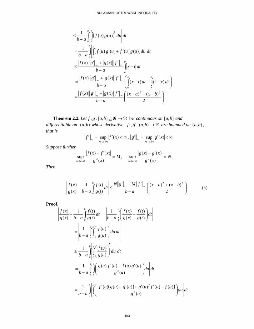
( ) dtduugufab
b
a
x
t∫ ∫ ′
−≤ )()(1
( ) dtduugufugufab
b
a
x
t∫ ∫ ′+′
−= )()()()(1
dttxab
fxggxf b
a∫ −
−
′+′≤ ∞∞
)()(
⎟⎟⎠
⎞⎜⎜⎝
⎛−+−
−
′+′= ∫ ∫∞∞
x
a
b
x
dtxtdttxab
fxggxf)()(
)()(
⎟⎟⎠
⎞⎜⎜⎝
⎛ −+−−
′+′= ∞∞
2)()()()( 22 bxax
abfxggxf
.
Theorem 2.2. Let ℜ→ℜ⊆],[:, bagf be continuous on ],[ ba and differentiable on ),( ba whose derivative ℜ→′′ ),(:, bagf are bounded on ),( ba , that is ∞<′=′∞<′=′
∈∞
∈∞
)(sup,)(sup),(),(
xggxffbaxbax
.
Suppose further
,)(
)()(sup,
)()()(
sup 2),(
2),(
Nxg
xgxgM
xgxfxf
baxbax=
′−=
′−
∈∈
Then
.2
)()()()(1
)()( 22
⎟⎟⎠
⎞⎜⎜⎝
⎛ −+−−
′+′≤
−− ∞∞∫
bxaxab
fMgNdt
tgtf
abxgxf b
a
(3)
Proof.
∫∫ ⎟⎟⎠
⎞⎜⎜⎝
⎛−
−=
−−
b
a
b
a
dttgtf
xgxf
abdt
tgtf
abxgxf
)()(
)()(1
)()(1
)()(
dtduuguf
ab
b
a
x
t∫ ∫
′
⎟⎟⎠
⎞⎜⎜⎝
⎛−
=)()(1
dtduuguf
ab
b
a
x
t∫ ∫
′
⎟⎟⎠
⎞⎜⎜⎝
⎛−
≤)()(1
dtduug
ugufufugab
b
a
x
t∫ ∫ ⎟⎟
⎠
⎞⎜⎜⎝
⎛ ′−′−
=)(
)()()()(12
( ) ( ) dtdu
ugufufuguguguf
ab
b
a
x
t∫ ∫ ⎟⎟
⎠
⎞⎜⎜⎝
⎛ −′′+′−′−
=)(
)()()()()()(12
SULAIMAN: OSTROWSKI INEQUALITY
103

dtduug
ufufugugugufab
b
a
x
t∫ ∫ ⎟⎟
⎠
⎞⎜⎜⎝
⎛ −′′+′−′
−≤
)()()()()()()(1
2
dttxab
fMgN b
a∫ −
−
′+′≤ ∞∞
.2
)()( 22
⎟⎟⎠
⎞⎜⎜⎝
⎛ −+−−
′+′= ∞∞ bxax
abfMgN
Theorem 2.3. Let ℜ→ℜ⊆],[: bag be continuous on ],[ ba and differentiable on ),( ba whose derivative ℜ→′ ),(: bag are bounded on ),( ba , that is ∞<′=′
∈∞
)(sup),(
xggbax
,
and let ( ) ℜ→],[: bagf be also continuous and has a bounded derivative, that is
( )∞<′=′
∈∞
)(sup],[
xffbagx
.
Then
.2
)()()(1)(22
⎟⎟⎠
⎞⎜⎜⎝
⎛ −+−−
′′≤
−− ∞∞∫
bxaxabgf
dttgfab
xgfb
a
οο (4)
Proof.
( )∫∫ −−
=−
−b
a
b
a
dttgfxgfab
dttgfab
xgf )()(1)(1)( οοοο
( ) dtduugfab
b
a
x
t∫ ∫ ′
−≤ )(1 ο
∫ ∫ ′′−
=b
a
x
t
dtduugugfab
)()((1
dtduabgf b
a
x
t∫ ∫−
′′≤ ∞∞
dttxabgf b
a∫ −
−
′′= ∞∞
.2
)()( 22
⎟⎟⎠
⎞⎜⎜⎝
⎛ −+−−
′′= ∞∞ bxax
abgf
Theorem 2.4. Let ℜ→ℜ⊆],[: baf is continuous on ],[ ba and differentiable on
),( ba whose derivative ℜ→′ ),(: baf is bounded on ),( ba , that is .)(sup
),(∞<′=′
∈∞
xffbax
Let .0 ba << Then
SULAIMAN: OSTROWSKI INEQUALITY
104

≤−
− ∫ ∫b
a
b
a
dsdtstfab
xyf )()(
1)( 2
( )( ) ( )( )( ) 2222222
)(2)()()()(
abf
bxaxabbyayxab−
′−+−−+−+−− ∞ . (5)
Proof.
∫ ∫−−
b
a
b
a
dsdtstfab
xyf )()(
1)( 2
( )dsdtstfxyfab
b
a
b
a∫ ∫ −
−= )()(
)(1
2
∫ ∫ ∫ ′−
=b
a
b
a
xy
st
dsdtduufab
)()(
12
dsdtduufab
b
a
b
a
xy
st∫ ∫ ∫ ′
−≤ )(
)(1
2
dsdtstxyab
f b
a
b
a∫ ∫ −
−
′≤ ∞
2)(
dsdtstxtxtxyab
f b
a
b
a∫ ∫ −+−
−
′= ∞
2)(
( )∫ ∫ −+−−
′≤ ∞
b
a
b
a
dsdtsxttyxab
f2)(
( ) ⎟⎟⎠
⎞⎜⎜⎝
⎛⎟⎟⎠
⎞⎜⎜⎝
⎛−⎟⎟
⎠
⎞⎜⎜⎝
⎛+−−
−
′= ∫∫∫∞
b
a
b
a
b
a
dttxdttdttyxabab
f)(
)( 2
( )( ) ( )( )( ) .)(2
)()()()( 2222222
abf
bxaxabbyayxab−
′−+−−+−+−−≤ ∞
Theorem 2.5. Let ℜ→ℜ⊆],[: baf is continuous on and bounded on ],[ ba that is .)(sup
],[∞<=
∈∞
xffbax
Define F by
∫=x
a
dttfxF .)()( (6)
Then
( ).)()()(2
)(1)( 22 bxaxab
fdttf
abxF
b
a
−+−−
≤−
− ∞∫ (7)
Proof.
( )∫∫ −−
=−
−b
a
b
a
dttFxFab
dttfab
xF )()(1)(1)(
SULAIMAN: OSTROWSKI INEQUALITY
105

dudtuFab
b
a
x
t∫ ∫ ′
−= )(1
dudtufab
b
a
x
t∫ ∫−
= )(1
dttxab
f b
a∫ −
−≤ ∞
( ).)()()(2
22 bxaxab
f−+−
−= ∞
Theorem 2.6. Let ℜ→ℜ⊆],[:, bagf be continuous on ],[ ba and differentiable on ),( ba whose derivative ℜ→′′ ),(:, bagf are bounded on ),( ba , that is ∞<′=′∞<′=′
∈∞
∈∞
)(sup,)(sup),(),(
xggxffbaxbax
.
Then
∫ ∫−−
−−
b
a
b
a
dttgab
xfdttfab
xgxgxf )()()()()()(2
( )22 )()()(2
)()(bxax
abgxffxg
−+−−
′+′≤ ∞∞ . (8)
Proof.
∫ ∫−−
−−
b
a
b
a
dttgab
xfdttfab
xgxgxf )()()()()()(2
( ) ( )∫ ∫ −−
+−−
=b
a
b
a
dttgxgab
xfdttfxfab
xg )()()()()()(
∫ ∫ ∫∫ ′−
+′−
=b
a
b
a
x
t
x
t
dtduugab
xfdtduufab
xg )()()()(
dttxab
gxffxg b
a∫ −
−
′+′≤ ∞∞
)()(
( ).)()()(2
)()( 22 bxaxab
gxffxg−+−
−
′+′= ∞∞
Theorem 2.7. Let ℜ→ℜ⊆],[:, bagf be continuous on ],[ ba and differentiable on ),( ba whose derivatives ℜ→++ ),(:, )1()1( bagf nm are bounded on
),( ba , that is ∞<=∞<= +
∈∞
++
∈∞
+ )(sup,)(sup )1(
),(
)1()1(
),(
)1( xggxff n
bax
nm
bax
m .
Then
SULAIMAN: OSTROWSKI INEQUALITY
106

( )∫ −−−
+b
a
mnnmnmnm dttfxgtgxftgtfab
xgxf )()()()()()(1)()( )()()()()()()()(
( ).)()()(3
33)1()1(
bxaxab
gf nm
−+−−
≤ ∞
+
∞
+
(9) Proof.
( )∫ −−−
+b
a
mnnmnmnm dttfxgtgxftgtfab
xgxf )()()()()()(1)()( )()()()()()()()(
( )∫ −−+−
=b
a
mnnmnmnm dttfxgtgxftgtfxgxfab
)()()()()()()()(1 )()()()()()()()(
( )( )∫ −−−
=b
a
nnmm dttgxgtfxfab
)()()()(1 )()()()(
dtduugduufab
x
t
nb
a
x
t
m ∫∫ ∫ ++
−≤ )()(1 )1()1(
∫ −−
≤ ∞
+
∞
+ b
a
nm
dttxab
gf2
)1()1(
)(
( ).)()()(3
33)1()1(
bxaxab
gf nm
−+−−
= ∞
+
∞
+
References
[1] D. S. Mitrinović, J. Pečarić and A. M. Fink, Inequalities involving functions and
Their Integrals and derivatives, Kluwer Academic publishers, Dordrecht, 1991.
SULAIMAN: OSTROWSKI INEQUALITY
107
Logarithmic order and type on some weighted
function spaces
A. El-Sayed AhmedTaif University , Faculty of Science Mathematics Department
Box 888 El-Hawiyah, El-Taif 5700, Saudi Arabia andSohag University, Faculty of Science, Department of Mathematics,
82524Sohag- Egypte-mail: [email protected]
A. KamalThe High Institute of Computer Science,
Al-Kawser city at Sohag Egypt
AbstractWe study the space QK,ω(p, q), of analytic functions on the unit disk in terms of a
nondecreasing function K. The relation between QK,ω(p, q) and Bq+2
pω spaces, which have
attracted considerable attention, is given by studying the growth order of K. The counterpartQ#
K,ω(p, q) of QK,ω(p, q) for the meromorphic case is also considered and investigated. Wenote that some characterizations of Q#
K,ω(p, q) and QK,ω(p, q) are different.
1 Introduction
Let D = z : |z| < 1 be the open unit disk in the complex plane C. Recall that the well known Bloch space (cf.[4]) is defined as follows:
B = f : f analytic in D and supz∈D
(1− |z|2)|f ′(z)| < ∞,
the little Bloch space B0 (cf. [4]) is a subspace of B consisting of all f ∈ B such that
lim|z|→1−
(1− |z|2)|f ′(z)| = 0.
The Dirichlet space is defined by
D = f : f analytic in D and
Z
D|f ′(z)|2dA(z) < ∞,
where dA(z) is the Euclidean area element dxdy. Let 0 < q < ∞. Then the Besov-type spaces
Bq =
(f : f analytic in D and sup
a∈D
Z
D|f ′(z)|q
1− |z|2
q−2
(1− |ϕa(z)|2)2dA(z) < ∞)
are introduced and studied intensively by Stroethoff (cf. [13]). Here, ϕa(z) stands for the Mobius transformationof D given by
ϕa(z) =a− z
1− az, where a ∈ D.
AMS: Primary 30D45 , Secondary 46E15.
Key words and phrases: QK,ω(p, q) spaces, Q#K,ω(p, q) spaces and α-weighted Bloch space.
1108
JOURNAL OF APPLIED FUNCTIONAL ANALYSIS, VOL.7, NO’S 1-2,108-117,COPYRIGHT 2012 EUDOXUS PRESS,LLC
2
In 1994, Aulaskari and Lappan [4] introduced a class of holomorphic functions, the so called Qp-spaces as follows:
Qp =
(f : f analytic in D and sup
a∈D
Z
D|f ′(z)|2gp(z, a)dA(z) < ∞
),
where 0 < p < ∞ and the weight function
g(z, a) = log
1− az
a− z
is defined as the composition of the Mobius transformation ϕa and the fundamental solution of the two-dimensionalreal Laplacian. The weight function g(z, a) is actually Green’s function in D with pole at a ∈ D.
For a point a ∈ D and 0 < r < 1, the pseudo-hyperbolic disk D(a, r) with pseudo-hyperbolic center a andpseudo-hyperbolic radius r is defined by D(a, r) = ϕa(rD).The pseudo-hyperbolic disk D(a, r) is also an Euclidean disk: its Euclidean center and Euclidean radius are(1−r2)a
1−r2|a|2 and (1−|a|2)r
1−r2|a|2 , respectively (see [13]). Let A denote the normalized Lebesgue area measure on D, and for
a Lebesgue measurable set K1 ⊂ D, denote by |K1| the measure of K1 with respect to A. It follows immediatelythat:
|D(a, r)| = (1− |a|2)2(1− r2|a|2)2 r2.
Let K : [0,∞) → [0,∞) be a nondecreasing function. For 0 < p < ∞, −2 < q < ∞, we say that a function fanalytic in D belongs to the space QK(p, q) (cf. [19]), if
‖f‖pQK(p,q) = sup
a∈D
Z
D|f ′(z)|p
1− |z|2
q
K(g(z, a))dA(z) < ∞.
Using the above mentioned function K, several authors have been studied some classes of holomorphic andmeromorphic function spaces (see [2, 7, 8, 10, 11, 15, 16, 17, 18, 19, 20] and others).Now, given a reasonable function ω : (0, 1] → (0,∞), the weighted Bloch space Bω (see [6]) is defined as the setof all analytic functions f on D satisfying
(1− |z|)|f ′(z)| ≤ Cω(1− |z|), z ∈ D,
for some fixed C = Cf > 0. In the special case where ω ≡ 1,Bω reduces to the classical Bloch space B. Here,the word ”reasonable” is a non-mathematical term; it was just intended to mean that the ”not too bad” and thefunction satisfy some natural conditions.Now, we introduce the following definitions:
Definition 1.1 For a given reasonable function ω : (0, 1] → (0,∞) and for 0 < α < ∞. An analytic function fon D is said to belong to the α−weighted Bloch space Bα
ω if
‖f‖Bαω
= supz∈D
(1− |z|)α
ω(1− |z|) |f′(z)| < ∞.
Definition 1.2 For a given reasonable function ω : (0, 1] → (0,∞) and for 0 < α < ∞. An analytic function fon D is said to belong to the little weighted Bloch space Bα
ω,0 if
‖f‖Bαω,0
= lim|z|→1−
(1− |z|)α
ω(1− |z|) |f′(z)| = 0.
Throughout this paper and for some techniques we consider the case of ω 6≡ 0.The logarithmic order (log-order) of the function K(r) is defined as
ρ = lim supr→∞
ln+ ln+ K(r)
ln r,
where ln+ x = maxln x, 0. If 0 < ρ < ∞, the logarithmic type (log-type) of the function K(r) is defined as
σ = lim supr→∞
ln+ K(r)
rρ.
Note that if f is an entire function, then the growth order of f is just the log-order of M(r), the maximummodulus function of f.
AHMED, KAMAL: WEIGHTED FUNCTION SPACES
109

3
Definition 1.3 [10, 11] For a nondecreasing function K : [0,∞) → [0,∞), 0 < p < ∞, −2 < q < ∞ and for agiven reasonable function ω : (0, 1] → (0,∞), an analytic function f in D is said to belong to the space QK,ω(p, q)if
‖f‖pQK,ω(p,q) = sup
a∈D
Z
D|f ′(z)|p
(1− |z|)qKg(z, a)
ωp(1− |z|) dA(z) < ∞.
Definition 1.4 For a given reasonable function ω : (0, 1] → (0,∞), and let 0 < p < ∞, −2 < q < ∞, 0 < s < ∞and an analytic function f in D is said to belong to the spaces Fω(p, q, s) if
‖f‖pFω(p,q,s) = sup
a∈D
Z
D|f ′(z)|p(1− |z|2)q gs(z, a)
ωp(1− |z|) dA(z) < ∞.
Moreover, if
lim|a|→1−
Z
D|f ′(z)|p(1− |z|2)q gs(z, a)
ωp(1− |z|) dA(z) = 0,
then f ∈ Fω,0(p, q, s).
Since every Mobius map ϕ can be written as ϕ(z) = eiθϕa(z), where θ is real.We assume throughout the paper that
1Z
0
(1− r2)−2K(log1
r)rdr < ∞.
We can define an auxiliary function as follows:
ϕK(s) = sup0<t≤1
K(st)
K(t), 0 < s < ∞.
Remark 1.1 It should be remarked that our QK,ω(p, q) classes are more general than many classes of analyticfunctions. If ω ≡ 1, we obtain QK(p, q) type spaces (cf. [18] and [19]). If q = p = 2, and ω(t) = t, we obtain QK
spaces as studied recently in [7, 8, 12, 16, 17, 20] and others. If q = p = 2, ω(t) = t and K(t) = tp, we obtain Qp
spaces as studied in [4, 5, 21] and others. If ω ≡ 1 and K(t) = ts, then QK,ω = F (p, q, s) classes (cf. [1, 22]).
2 Analytic classes QK,ω(p, q)
We first give some basic properties of analytic QK,ω(p, q) spaces.
Proposition 2.1 Let K : [0,∞) → [0,∞) be a nondecreasing function and ω : (0, 1] → (0,∞), where ω(λt) =λω(t). For 0 < p < ∞ and −2 < q < ∞, we have that the spaces QK,ω(p, q) are subset of the weighted Bloch space
Bq+2
pω .
Proof: For a fixed r ∈ (0, 1) and a ∈ D, let
E(a, r) =
(z ∈ D, |z − a| < r(1− |a|)
).
Also, suppose that f ∈ QK,ω(p, q), we obtain
‖f‖pQK,ω(p,q) = sup
a∈D
Z
D|f ′(z)|p(1− |z|)q K(g(z, a))
ωp(1− |z|) dA(z)
≥Z
D|f ′(z)|p
1− |z|2
q K(g(z, a))
ωp(1− |z|)dA(z)
≥Z
D(a,r)
|f ′(z)|p1− |z|2
q K(g(z, a))
ωp(1− |z|)dA(z)
≥ K(log1
r)
Z
D(a,r)
|f ′(z)|p (1− |z|2)q
ωp(1− |z|)dA(z)
≥ K(log1
r)
Z
E(a,r)
|f ′(z)|p (1− |z|2)q
ωp(1− |z|)dA(z).
AHMED, KAMAL: WEIGHTED FUNCTION SPACES
110

4
We know that E(a, r) ⊂ D(a, r) and for any z ∈ E(a, r), we have
(1− r)(1− |a|) ≤ 1− |z| ≤ (1 + r)(1− |a|),then,
(1− |z|)p ≥ (1− r)p(1− |a|)p , ∀ p > 0.
Now, since we assume that ω is non-decreasing, then we obtain that
‖f‖pQK,ω(p,q) ≥ K(log
1
r)
Z
E(a,r)
|f ′(z)|p (1− |z|2)q
ωp(1− |z|)dA(z)
≥ K(log 1r)(1− r)p(1− |a|)q
ωp((1− r)(1− |a|))Z
E(a,r)
|f ′(z)|pdA(z)
Since |f ′(z)|p is a subharmonic function, thenZ
E(a,r)
|f ′(z)|p dA(z) ≥ |E(a, r)| |f ′(a)|p = r2(1− |a|)2|f ′(a)p
.
Then we obtain
‖f‖pQK,ω(p,q) ≥ K(log 1
r)(1− r)p−1(1− |a|)q+2
ωp((1− r)(1− |a|)) |f ′(a)|p
≥ C1
K(log 1r)(1− r)p(1− |a|)q+2
ωp((1− |a|)) |f ′(a)|p
which implies that
‖f‖p
Bq+2
pω
≤‖f‖p
QK,ω(p,q)
C1(1− r)p−1K(log 1r). (1)
Our proposition is therefore established.
Next, we give the following proposition.
Proposition 2.2 If the log-order ρ and the log-type σ of a nondecreasing function K(r) satisfy one of the followingconditions:(i) ρ > 1(ii) ρ = 1 and 0 < σ < ∞,then ‖f‖p
QK,ω(p,q) ⊂ ‖f‖p
Bq+2
pω
, where 0 < p < ∞, −2 < q < ∞ and ω : (0, 1] → (0,∞).
Proof: By Proposition 2.1, it suffices to show that each non-constant weighted α-Bloch function f can not belongto the spaces QK,ω(p, q).In fact, if either the log-order ρ of K(r) is greater than 0, or the log-order ρ of K(r) equals 1 and the log-type σof K(r) is greater than 2, then there exists a sequence rn with rn →∞ as n →∞ such that
limn→∞
ln+ ln+ K(rn)
ln rn= ρ > 1 (2)
or
σ = limn→∞
ln+ K(rn)
rn= λ > 0 (3)
In the case (2) or (3), we obtain
limn→∞
K(rn)
eλrn= const. (4)
Let f be a non-constant weighted α-Bloch function. Then
‖f‖p
Bq+2
pω
= supz∈D
(1− |z|2)q
ωp(1− |z|) |f′(z)|p : z ∈ D 6= 0.
However, by (1) and (4) we have
‖f‖pQK,ω(p,q) = sup
a∈D
Z
D|f ′(z)|p
1− |z|2
q K(g(z, a))
ωp(1− |z|)dA(z)
≥ π‖f‖p
Bq+2
pω
(1− tn)pK(log1
tn) 6→ ∞.
Hence, f ∈ QK,ω(p, q).
AHMED, KAMAL: WEIGHTED FUNCTION SPACES
111
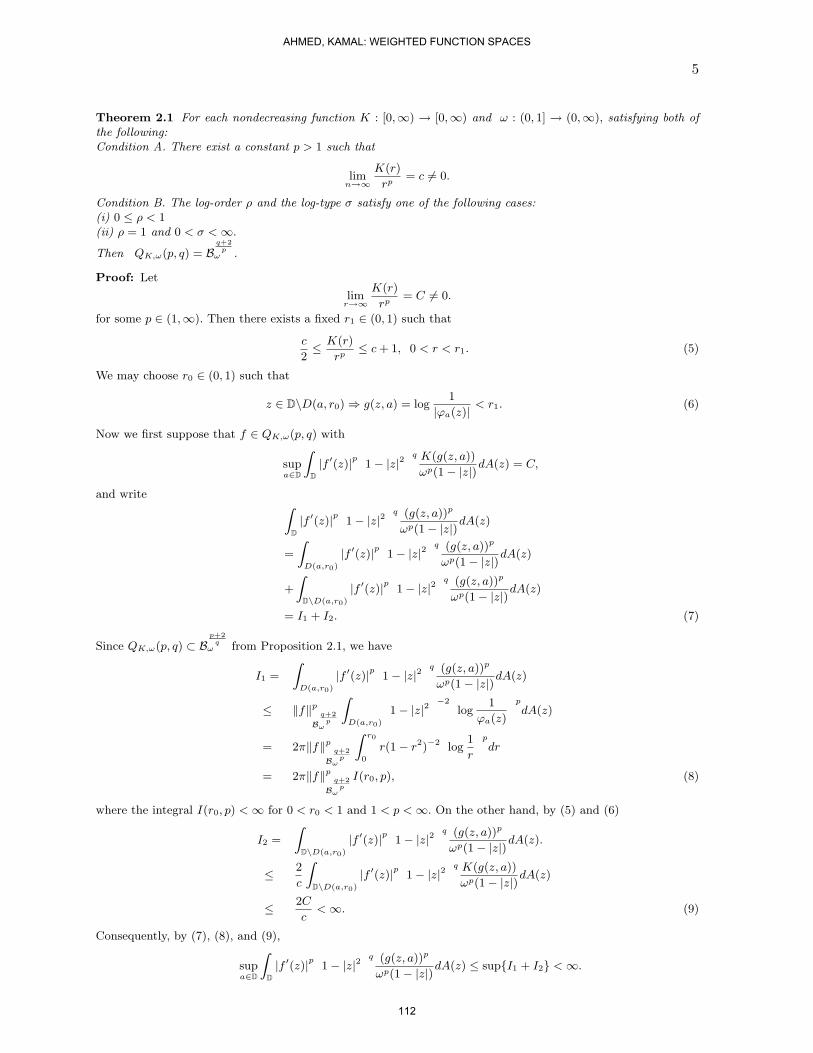
5
Theorem 2.1 For each nondecreasing function K : [0,∞) → [0,∞) and ω : (0, 1] → (0,∞), satisfying both ofthe following:Condition A. There exist a constant p > 1 such that
limn→∞
K(r)
rp= c 6= 0.
Condition B. The log-order ρ and the log-type σ satisfy one of the following cases:(i) 0 ≤ ρ < 1(ii) ρ = 1 and 0 < σ < ∞.
Then QK,ω(p, q) = Bq+2
pω .
Proof: Let
limr→∞
K(r)
rp= C 6= 0.
for some p ∈ (1,∞). Then there exists a fixed r1 ∈ (0, 1) such that
c
2≤ K(r)
rp≤ c + 1, 0 < r < r1. (5)
We may choose r0 ∈ (0, 1) such that
z ∈ D\D(a, r0) ⇒ g(z, a) = log1
|ϕa(z)| < r1. (6)
Now we first suppose that f ∈ QK,ω(p, q) with
supa∈D
Z
D|f ′(z)|p
1− |z|2
q K(g(z, a))
ωp(1− |z|)dA(z) = C,
and writeZ
D|f ′(z)|p
1− |z|2
q (g(z, a))p
ωp(1− |z|)dA(z)
=
Z
D(a,r0)
|f ′(z)|p1− |z|2
q (g(z, a))p
ωp(1− |z|)dA(z)
+
Z
D\D(a,r0)
|f ′(z)|p1− |z|2
q (g(z, a))p
ωp(1− |z|)dA(z)
= I1 + I2. (7)
Since QK,ω(p, q) ⊂ Bp+2
qω from Proposition 2.1, we have
I1 =
Z
D(a,r0)
|f ′(z)|p1− |z|2
q (g(z, a))p
ωp(1− |z|)dA(z)
≤ ‖f‖p
Bq+2
pω
Z
D(a,r0)
1− |z|2
−2log
1
ϕa(z)
p
dA(z)
= 2π‖f‖p
Bq+2
pω
Z r0
0
r(1− r2)−2log
1
r
p
dr
= 2π‖f‖p
Bq+2
pω
I(r0, p), (8)
where the integral I(r0, p) < ∞ for 0 < r0 < 1 and 1 < p < ∞. On the other hand, by (5) and (6)
I2 =
Z
D\D(a,r0)
|f ′(z)|p1− |z|2
q (g(z, a))p
ωp(1− |z|)dA(z).
≤ 2
c
Z
D\D(a,r0)
|f ′(z)|p1− |z|2
q K(g(z, a))
ωp(1− |z|)dA(z)
≤ 2C
c< ∞. (9)
Consequently, by (7), (8), and (9),
supa∈D
Z
D|f ′(z)|p
1− |z|2
q (g(z, a))p
ωp(1− |z|)dA(z) ≤ supI1 + I2 < ∞.
AHMED, KAMAL: WEIGHTED FUNCTION SPACES
112
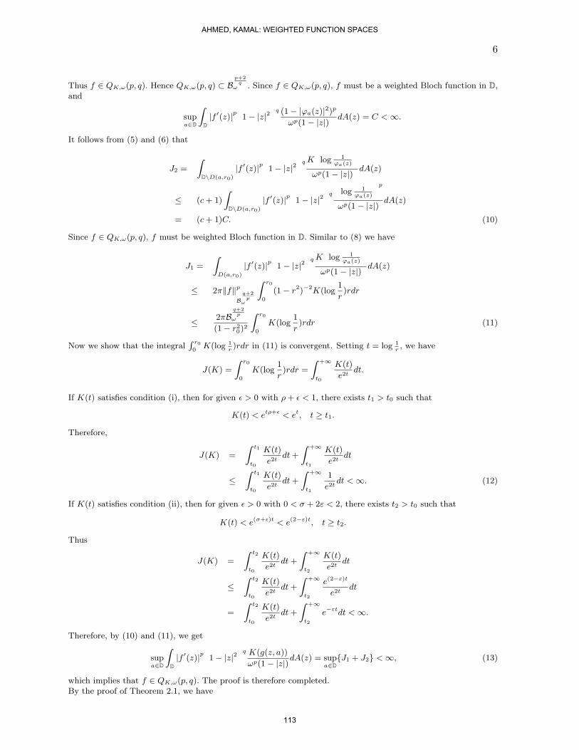
6
Thus f ∈ QK,ω(p, q). Hence QK,ω(p, q) ⊂ Bp+2
qω . Since f ∈ QK,ω(p, q), f must be a weighted Bloch function in D,
and
supa∈D
Z
D|f ′(z)|p
1− |z|2
q (1− |ϕa(z)|2)p
ωp(1− |z|) dA(z) = C < ∞.
It follows from (5) and (6) that
J2 =
Z
D\D(a,r0)
|f ′(z)|p1− |z|2
q Klog 1
ϕa(z)
ωp(1− |z|) dA(z)
≤ (c + 1)
Z
D\D(a,r0)
|f ′(z)|p1− |z|2
q
log 1
ϕa(z)
p
ωp(1− |z|) dA(z)
= (c + 1)C. (10)
Since f ∈ QK,ω(p, q), f must be weighted Bloch function in D. Similar to (8) we have
J1 =
Z
D(a,r0)
|f ′(z)|p1− |z|2
q Klog 1
ϕa(z)
ωp(1− |z|) dA(z)
≤ 2π‖f‖p
Bq+2
pω
Z r0
0
(1− r2)−2K(log1
r)rdr
≤ 2πBq+2
pω
(1− r20)
2
Z r0
0
K(log1
r)rdr (11)
Now we show that the integralR r00
K(log 1r)rdr in (11) is convergent. Setting t = log 1
r, we have
J(K) =
Z r0
0
K(log1
r)rdr =
Z +∞
t0
K(t)
e2tdt.
If K(t) satisfies condition (i), then for given ε > 0 with ρ + ε < 1, there exists t1 > t0 such that
K(t) < etρ+ε < et, t ≥ t1.
Therefore,
J(K) =
Z t1
t0
K(t)
e2tdt +
Z +∞
t1
K(t)
e2tdt
≤Z t1
t0
K(t)
e2tdt +
Z +∞
t1
1
e2tdt < ∞. (12)
If K(t) satisfies condition (ii), then for given ε > 0 with 0 < σ + 2ε < 2, there exists t2 > t0 such that
K(t) < e(σ+ε)t < e(2−ε)t, t ≥ t2.
Thus
J(K) =
Z t2
t0
K(t)
e2tdt +
Z +∞
t2
K(t)
e2tdt
≤Z t2
t0
K(t)
e2tdt +
Z +∞
t2
e(2−ε)t
e2tdt
=
Z t2
t0
K(t)
e2tdt +
Z +∞
t2
e−εtdt < ∞.
Therefore, by (10) and (11), we get
supa∈D
Z
D|f ′(z)|p
1− |z|2
q K(g(z, a))
ωp(1− |z|)dA(z) = supa∈D
J1 + J2 < ∞, (13)
which implies that f ∈ QK,ω(p, q). The proof is therefore completed.By the proof of Theorem 2.1, we have
AHMED, KAMAL: WEIGHTED FUNCTION SPACES
113

7
Corollary 2.1 Let K : [0,∞) → [0,∞) be a nondecreasing function. If K(r) satisfies Condition A in Theorem
2.1 for some p, 1 < p < ∞, then QK,ω(p, q) ⊂ Bq+2
pω .
Remark 2.1 In the case p > 1, we know that QK,ω(p, q) = Bq+2
pω (see [11]), but now we have always that
QK,ω(p, q) ⊂ Bq+2
pω .
Corollary 2.2 Let K : [0,∞) → [0,∞) be a bounded and nondecreasing function. If
limr→0
K(r)
rp= C 6= ∞.
holds for some p > 1, then QK,ω(p, q) = Bq+2
pω .
3 Meromorphic classes Q#K,ω(p, q)
For a meromorphic function f a natural analogue of |f ′(z)| is the spherical derivative
f#(z) =|f ′(z)|
(1 + |f(z)|2) .
Corresponding to the definitions of the spaces Fω(p, q, s) and Fω,0(p, q, s), we define the classes F#ω (p, q, s) and
F#ω,0(p, q, s) as follows:
Definition 3.1 Let 0 < p < ∞, −2 < q < ∞ and 0 ≤ s < ∞. A function f meromorphic in D is said to belongto the class F#
ω (p, q, s) if
‖f‖p
F#ω p,q,s
= supa∈D
Z
D
f#(z)
p1− |z|2
q gs(z, a)
ωp(1− |z|)dA(z) < ∞.
Moreover, if
‖f‖p
F#ω,0p,q,s
= lim|a|→1−
Z
D
f#(z)
p1− |z|2
q gs(z, a)
ωp(1− |z|)dA(z) = 0,
then f ∈ F#ω (p, q, s).
Therefore we define the classes M#ω (p, q, s) and M#
ω,0(p, q, s) as follows.
Definition 3.2 Let 0 < p < ∞, −2 < q < ∞ and 0 ≤ s < ∞. A function f meromorphic in D is said to belongto the class M#
ω (p, q, s) if
‖f‖p
M#ω p,q,s
= supa∈D
Z
D
f#(z)
p1− |z|2
q (1− |ϕa(z)|2)s
ωp(1− |z|) dA(z) < ∞.
Moreover, if
‖f‖p
M#ω,0p,q,s
= lim|a|→1−
Z
D
f#(z)
p1− |z|2
q (1− |ϕa(z)|2)s
ωp(1− |z|) dA(z) = 0,
then f ∈ M#ω (p, q, s).
Let Nαω be the class of all normal functions in D. We recall that a function f meromorphic in D is called to be
normal if and only if
supz∈D
(1− |z|2)α
ω(1− |z|) f#(z) < ∞.
We will need the following theorem in future:
Theorem 3.1 [14, 15] Let 2 ≤ q < ∞, and let 0 < p < ∞ and let 0 < r < 1. Then a function f meromorphic inD is normal if and only if
supa∈D
Z
D
f#(z)
q1− |z|2
q−2g(z, a)
p
dA(z) < ∞.
Now, we give the following theorem.
AHMED, KAMAL: WEIGHTED FUNCTION SPACES
114
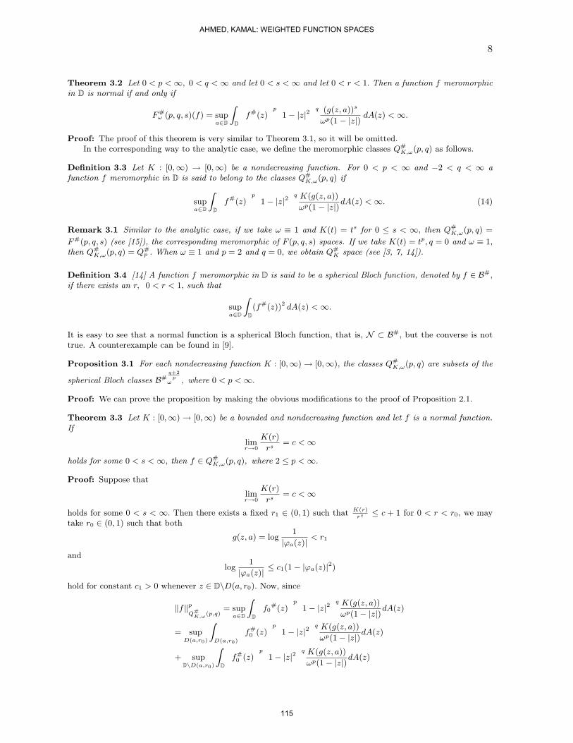
8
Theorem 3.2 Let 0 < p < ∞, 0 < q < ∞ and let 0 < s < ∞ and let 0 < r < 1. Then a function f meromorphicin D is normal if and only if
F#ω (p, q, s)(f) = sup
a∈D
Z
D
f#(z)
p1− |z|2
q (g(z, a))s
ωp(1− |z|) dA(z) < ∞.
Proof: The proof of this theorem is very similar to Theorem 3.1, so it will be omitted.In the corresponding way to the analytic case, we define the meromorphic classes Q#
K,ω(p, q) as follows.
Definition 3.3 Let K : [0,∞) → [0,∞) be a nondecreasing function. For 0 < p < ∞ and −2 < q < ∞ afunction f meromorphic in D is said to belong to the classes Q#
K,ω(p, q) if
supa∈D
Z
D
f#(z)
p1− |z|2
q K(g(z, a))
ωp(1− |z|)dA(z) < ∞. (14)
Remark 3.1 Similar to the analytic case, if we take ω ≡ 1 and K(t) = ts for 0 ≤ s < ∞, then Q#K,ω(p, q) =
F#(p, q, s) (see [15]), the corresponding meromorphic of F (p, q, s) spaces. If we take K(t) = tp, q = 0 and ω ≡ 1,then Q#
K,ω(p, q) = Q#p . When ω ≡ 1 and p = 2 and q = 0, we obtain Q#
K space (see [3, 7, 14]).
Definition 3.4 [14] A function f meromorphic in D is said to be a spherical Bloch function, denoted by f ∈ B#,if there exists an r, 0 < r < 1, such that
supa∈D
Z
D(f#(z))2 dA(z) < ∞.
It is easy to see that a normal function is a spherical Bloch function, that is, N ⊂ B#, but the converse is nottrue. A counterexample can be found in [9].
Proposition 3.1 For each nondecreasing function K : [0,∞) → [0,∞), the classes Q#K,ω(p, q) are subsets of the
spherical Bloch classes B#q+2
pω , where 0 < p < ∞.
Proof: We can prove the proposition by making the obvious modifications to the proof of Proposition 2.1.
Theorem 3.3 Let K : [0,∞) → [0,∞) be a bounded and nondecreasing function and let f is a normal function.If
limr→0
K(r)
rs= c < ∞
holds for some 0 < s < ∞, then f ∈ Q#K,ω(p, q), where 2 ≤ p < ∞.
Proof: Suppose that
limr→0
K(r)
rs= c < ∞
holds for some 0 < s < ∞. Then there exists a fixed r1 ∈ (0, 1) such that K(r)rs ≤ c + 1 for 0 < r < r0, we may
take r0 ∈ (0, 1) such that both
g(z, a) = log1
|ϕa(z)| < r1
and
log1
|ϕa(z)| ≤ c1(1− |ϕa(z)|2)
hold for constant c1 > 0 whenever z ∈ D\D(a, r0). Now, since
‖f‖p
Q#K,ω
(p,q)= sup
a∈D
Z
D
f0
#(z)p
1− |z|2q K(g(z, a))
ωp(1− |z|)dA(z)
= supD(a,r0)
Z
D(a,r0)
f#0 (z)
p1− |z|2
q K(g(z, a))
ωp(1− |z|)dA(z)
+ supD\D(a,r0)
Z
D
f#0 (z)
p1− |z|2
q K(g(z, a))
ωp(1− |z|)dA(z)
AHMED, KAMAL: WEIGHTED FUNCTION SPACES
115

9
For a ∈ D and r0 as above, then using Theorem 3.2, we have that
L2 =
Z
D\D(a,r0)
f#0 (z)
p1− |z|2
q K(g(z, a))
ωp(1− |z|)dA(z)
≤ (c + 1)(c1)s
Z
D\D(a,r0)
f#0 (z)
p1− |z|2
q (1− |ϕa(z)|2)s
ωp(1− |z|) dA(z)
≤ (c + 1)(c1)s F#
ω (p, q, s) < ∞. (15)
On the other hand, since K is bounded, there exists a constant C2 such that K(r) ≤ C2 for all r : 0 < r < ∞.Thus
L1 =
Z
D(a,r0)
f#0 (z)
p1− |z|2
q K(g(z, a))
ωp(1− |z|)dA(z)
≤ C2
(1− r20)
s
Z
D(a,r0)
f#0 (z)
p1− |z|2
q (1− |ϕa(z)|2)s
ωp(1− |z|) dA(z)
=C2
(1− r20)
sF#
ω (p, q, s). (16)
Therefore, by (15) and (16), we have
supa∈D
Z
D
f#0 (z)
p1− |z|2
q K(1− |ϕa(z)|2)ωp(1− |z|) dA(z) = sup
a∈DL1 + L2 < ∞.
Thus f0 ∈ ‖f‖p
Q#k,ω(p,q)
, the proof of our theorem is completed.
Finally, we consider the harmonic counterpart of QK,ω(p, q) as follows:
Definition 3.5 Let K : [0,∞) → [0,∞) be a nondecreasing function. A function u real-valued harmonic in D issaid to belong to the space QKh,ω(p, q) if
supa∈D
Z
D|∇u(z)|p
1− |z|2
q K(g(z, a))
ωp(1− |z|)dA(z) < ∞,
where ∇u(z) = (ux, uy) is the gradient of u and |∇u(z)| =pu2x + u2
y, 0 < p < ∞ and −2 < q < ∞.Note that if we take K(r) = rp for 0 < p < ∞, then QKh,ω(p, q) is a harmonic weighted Bloch space Bα
h,ω, where
Bαh,ω = u : u harmonic in D and sup
z∈D
(1− |z|2)α|∇u(z)|ω(1− |z|) < ∞.
It is easy to see that some corresponding results to Propositions 2.1, 2.2, and Theorem 2.1 are also true forQKh,ω(p, q) and the proof are similar to those of them.
Remark 3.2 It should be remarked that our results in this paper are completely different from that introduced byWulan et. al in [19], since the authors in [19] introduced their characterizations without use of the logarithmicorder and logarithmic type of a nondecreasing function. On the other hand , we introduced some results in thesense of meromorphic and harmonic functions.
References
[1] A. El-Sayed Ahmed and M. A. Bahkit, Composition operators on some holomorphic Banach function spaces,Mathematica Scandinavica, 104(2)(2009), 275-295.
[2] A. El-Sayed Ahmed and M. A. Bahkit, Hadamard products and NK space, Mathematical and computerModelling, 51(1-2)(2010), 33-43.
[3] A. El-Sayed Ahmed and M. A. Bahkit, Sequences of some meromorphic function spaces, Bull.Belg. Math.Soc.- Simon Stevin, Vol 16(3)(2009), 395-408.
[4] R. Aulaskari, and P. Lappan, Criteria for an analytic function to be Bloch and a harmonic or meromorphicfunction to be normal, Complex Analysis and its Applications (eds Y. Chung-Chun et al.), Pitman ResearchNotes in Mathematics 305, Longman (1994), 136-146.
AHMED, KAMAL: WEIGHTED FUNCTION SPACES
116
10
[5] R. Aulaskari, and L. Tovar, On the function spaces Bp and Qp. Bull. Hong Kong. Math. Soc. 1(1997),203-208.
[6] K. M. Dyakonov, Weighted Bloch spaces, Hp, and BMOA, J. Lond. Math. Soc. II. Ser. 65(2)(2002), 411-417.
[7] M. Essen and H. Wulan, On analytic and meromorphic functions and spaces of QK type, Illinois J. Math.46(2002), 1233-1258.
[8] M. Essen, H. Wulan, and J. Xiao, Several Function-theoretic characterizations of Mobius invariant QK spaces,J. Funct. Anal. 230 (2006), 78-115.
[9] P. Lappan, A non-normal locally uniformly univalent function, Bull. London Math. Soc. 5(1973), 491-495.
[10] R. A. Rashwan, A. El-Sayed Ahmed and Alaa Kamal, Some characterizations of weighted holomorphic Blochspace, European Journal of Pure and applied Mathematics, Vol.2(2)(2009), 250-267.
[11] R. A. Rashwan, A. El-Sayed Ahmed and Alaa Kamal, Integral characterizations of weighted Bloch space andQK,ω(p, q) spaces, Mathematica, Tome 51 (74), N 1, 2009, 6376.
[12] S. Li Songxiao and H. Wulan, Composition operators on QK spaces, J. Math. Anal. Appl. 327(2)(2007),948-958.
[13] K. Stroethoff, Besov-type characterisations for the Bloch space, Bull. Austral. Math. Soc. 39(1989), 405-420.
[14] H. Wulan, On some classes of meromorphic functions, Ann. Acad. Sci. Fenn. Ser.A Math. Diss.116(1998),1-57.
[15] H. Wulan, some problems on normal and little normal functions, Complex variables, 36(3)(1998),301-309.
[16] H. Wulan and P. Wu, Characterizations of QT spaces, J. Math. Anal. Appl. 254(2001), 484-497.
[17] H. Wulan and Y. Zhang, Hadamard products and QK spaces, J. Math. Anal. Appl. 337(2008), 1142-1150.
[18] H. Wulan and J. Zhou, The higher order derivatives of QK type spaces, J. Math. Anal. Appl. 332(2)(2007),1216-1228.
[19] H. Wulan and K. Zhu, QK type spaces of analytic functions, J. Funct. Spaces Appl. 4(2006), 73-84.
[20] H. Wulan and K. Zhu, Derivative-free characterizations of QK spaces, J. Aust. Math. Soc. 82(2)(2007),283-295.
[21] J. Xiao, Holomorphic Q Classes, Springer LNM 1767, Berlin, 2001.
[22] R. Zhao, On a general family of function spaces, Ann. Acad. Sci. Fenn. Math. Diss. 105, 1996.
AHMED, KAMAL: WEIGHTED FUNCTION SPACES
117

SOME FIXED POINT THEOREM FOR MAPPING ONCOMPLETE G-CONE METRIC SPACES
DURAN TURKOGLU AND NURCAN BILGILI
Abstract. In this paper we introduce G-cone metric spaces and we give someproperties about this spaces. Further we prove some xed point results formapping satisfying su¢ cient conditions on complete G-cone metric space,thenwe showed that if the G-cone metric space (X;G) is symmetric ,the existenceand uniqueness of these xed point results follow from well-known theoremsin cone metric space (X; dG),where (X; dG) is the cone metric space whichdened from the G-cone metric space (X;G).
1. introduction
Cone metric spaces were introduced by Huang and Zhang in [4]. The authorsthere described convergence in cone metric spaces and introduced completeness.Then they proved some xed point theorems of contractive mappings on cone met-ric spaces. Some denitions and topological concepts were generalized in [2] andthey proved there that every cone metric space is a topological space, they alsogeneralized the concept of diametrically contractive mappings and proved somexed point theorems in cone metric spaces. Furthermore, cone metric spaces werestudied by many authors (see [1, 3, 5, 6, 7, 8, 9, 10, 11, 12, 13]).On the other hand, during the sixties, the notion of 2-metric space introduced by
Gähler (see [14, 15])as a generalization of usual notion of metric space (X; d).Butdi¤erent authors proved that there is no relation between these two functions, forinstance, Ha et al.in [16] show that 2-metric need not be continuous function, furtherthere is no easy relationship between results obtained in the two settings.In 1992, Bapure Dhage in his Ph.D.thesis introduce a new class of generalized
metric space called D-metric spaces .([17, 18])In a subsequent series of papers, Dhage attempted to develop topological struc-
tures in such spaces (see [18, 19]). He claimed that D-metrics provide a gener-alization of ordinary metric functions and went on to present several xed pointresults.But in 2003 Zead Mustafa and Brailey Sims demonstrated in [20] that most of
the claims concerning the fundamental topological structure of D-metric space areincorrect, so, were introduced more appropriate notion of generalized metric spacein [21] and they proved some xed point results for mapping satisfying su¢ cientconditions on complete G-metric space.In this paper we introduce G-cone metric spaces, we give some properties about
this spaces and we prove some xed point results for mapping satisfying su¢ cientconditions on complete G-cone metric spaces.
2000 Mathematics Subject Classication. Primary 47H10, Secondary 54H25.Key words and phrases. xed point, cone metric space, G-metric.
1
118
JOURNAL OF APPLIED FUNCTIONAL ANALYSIS, VOL.7, NO’S 1-2,118-137,COPYRIGHT 2012 EUDOXUS PRESS,LLC

2 DURAN TURKOGLU AND NURCAN BILGILI
2. G-cone metric spacesIn this section we shall dene G-cone metric spaces and prove some properties.Let E always be a real Banach space and P a subset of E. P is called a cone if
and only if(i) P is closed, nonempty, and P 6= fg;(ii) a; b 2 R; a; b 0; x; y 2 P ) ax+ by 2 P ;(iii) x 2 P and x 2 P ) x = .Given a cone P E, we dene a partial ordering with respect to P by x y
if and only if y x 2 P . We shall write x < y to indicate that x y but x 6= y,while x << y will stand for y x 2 intP , intP denotes the interior of P. Thecone P is called normal if there is a number K 1 such that for all x; y 2 E, x y implies kxk K kyk. The least positive number satisfying above iscalled the normal constant of P .In the following we always suppose E is a real Banach space, P is cone in E with
intP 6= ? and is partial ordering with respect to P .
Denition 1. Let X be a nonempty set , and let G : X X X ! E be afunction satisfying the following properties:(G1) G (x; y; z) = if and only if x = y = z;(G2) < G (x; x; y); for all x; y 2 X, with x 6= y;(G3) G (x; x; y) G (x; y; z), for all x; y; z 2 X, with z 6= y;(G4) G (x; y; z) = G (x; z; y) = G (y; z; x) = :::, (symmetry in all three variables);(G5) G (x; y; z) G (x; a; a) + G (a; y; z), for all x; y; z; a 2 X, (rectangle in-
equality).Then the function G is called a generalized cone metric , or, more specically, a
G -cone metric on X, and the pair (X;G) is called a G-cone metric space.
Denition 2. Let (X;G) be a G-cone metric space. Let (xn) be a sequence in Xand x 2 X. If for every c 2 E with << c there is N 2 N such that for alln;m N , G (x; xn; xm) << c, then (xn) is said to be G-cone convergent to x in Xand x is limit of (xn). We denote this by lim
n;m!1xn = x or xn ! x (n;m !1)
Lemma 1. Let (X;G) be a G-cone metric space. Then for c 2 E with << c,there is > 0 such that kxk < implies c x 2 intP:
Proof. Since c >> , then c 2 intP . Hence nd > 0 such that N (c) =fx 2 E : kx ck < g intP . ( Sincekc ck = < ; thenc 2 N (c) so N (c) 6= ? ). Now if kxk < then kx c+ ck < hence,
j1j kx c+ ck = kx+ c ck = k(c x) ck < then c x 2 N (c) intPand so, c x 2 intP:
Lemma 2. Let (X;G) be a G-cone metric space, P be a normal cone with normalconstant K. Let (xn) be a sequence in X. Then (xn) is G-cone convergent to x ifand only if G (x; xn; xm) ! (n;m !1).
Proof. Suppose that (xn) is G-cone convergent to x. For every real " > 0, choosec 2 E with << c and K kck < ". Then there is N 2 N, for all n;m N ,G (x; xn; xm) << c. Since P is a normal cone with normal constantK, when n;m N , kG (x; xn; xm)k K kck < ". This means G (x; xn; xm) ! (n;m !1) orlim
n;m!1G (x; xn; xm)=.
119

SOME FIXED POINT THEOREM FOR MAPPING ON COMPLETE G-CONE METRIC SPACES 3
Conversely, suppose that G (x; xn; xm) ! (n;m !1). From Lemma 1 forevery c 2 E with << c, there is > 0 such that kxk < implies c x 2intP . For this there is N 2 N, such that for all n;m N , kG (x; xn; xm)k < .So c G (x; xn; xm) 2 intP . This means G (x; xn; xm) << c. Therefore (xn) isG-cone convergent to x. Lemma 3. Let (X;G) be a G-cone metric space, P be a normal cone with normalconstant K. Then the following are equivalent.(1) (xn) is G-cone convergent to x.(2) G (xn; xn; x) ! , as n !1.(3) G (xn; x; x) ! , as n !1.(4) (xm; xn; x) ! , as m;n !1.
Proof. (1) =) (2) :Suppose that (xn) is G-cone convergent to x. From Lemma 2, G (x; xn; xm) !
(n;m !1). If we choosem = n, then G (x; xn; xn) ! (n !1). From (G4),G (x; xn; xn) = G (xn; xn; x) so G (xn; xn; x) ! , as n !1.(2) =) (3) :Suppose that G (xn; xn; x) ! , as n !1. If we choose a = xn in (G5), then
G (x; xn; x) G (x; xn; xn)+G (xn; xn; x). From (G4), G (xn; xn; x) = G (x; xn; xn)and since G (xn; xn; x) ! , as n !1, for any " > 0, there is N 2 N such thatfor all n N ,kG (xn; xn; x)k < "
2K . Since P is a normal cone with normal constantK,
kG (x; xn; x)k K kG (x; xn; xn) +G (xn; xn; x)k= K (kG (x; xn; xn)k+ kG (xn; xn; x)k)
< K "
2K+
"
2K
= ":
From (G4), G (xn; x; x) = G (x; xn; x) so for any " > 0, there is N 2 N such thatfor all n N , kG (xn; x; x)k < ".This means G (xn; x; x) ! , as n !1.(3) =) (4) :Suppose that G (xn; x; x) ! ,as n ! 1. If we choose a = x in (G5), then
G (xm; xn; x) G (xm; x; x) + G (x; xn; x). Since G (xn; x; x) ! , as n ! 1and from (G4),G (xm; x; x) ! and G (xn; x; x) = G (x; xn; x) ! . So forany " > 0, there is N 2 N such that for all n;m N , kG (xm; x; x)k < "
2K ,kG (x; xn; x)k < "
2K . Since P is a normal cone with normal constant K,
kG (xm; xn; x)k K kG (xm; x; x) +G (x; xn; x)k= K (kG (xm; x; x)k+ kG (x; xn; x)k)
< K "
2K+
"
2K
= ":
So for any " > 0, there is N 2 N such that for all n;m N , kG (xm; xn; x)k < ".This means G (xm; xn; x) ! , as m;n !1.(4) =) (1) :Suppose that G (xm; xn; x) ! , as m;n ! 1. From (G4),G (xm; xn; x) =
G (x; xn; xm). So from Lemma 2, (xn) is G-cone convergent to x. Lemma 4. Let (X;G) be a G-cone metric space, P be a normal cone with normalconstant K. Let (xn) be a sequence in X. If (xn) is G-cone convergent to x and(xn) is G-cone convergent to y, then x = y. That is the limit of (xn) is unique.
120

4 DURAN TURKOGLU AND NURCAN BILGILI
Proof. From xn ! x and xn ! y (n;m !1), for any c 2 E with << c thereis N 2 N such that for all n;m N , G (x; xn; xm) << c and G (y; xn; xm) << c.If we choose a = xm in (G5), then
G (x; xn; y) G (x; xm; xm) +G (xm; xn; y)
c+ c = 2c
and we choose a = xn in (G5), then
G (x; x; y) G (x; xn; xn) +G (xn; x; y)
c+ 2c = 3c:
Since P is a normal cone with normal constant K, kG (x; x; y)k 3K kck. Since cis arbitrary G (x; x; y) = , therefore x = y:
Denition 3. Let (X;G) be a G-cone metric space. Let (xn) be a sequence inX. If for every c 2 E with << c there is N 2 N such that for all n;m; l N ,G (xn; xm; xl) << c, then (xn) is called a G-cone Cauchy sequence in X.
Lemma 5. Let (X;G) be a G-cone metric space, P be a normal cone with normalconstant K. Let (xn) be a sequence in X. Then (xn) is a G-cone Cauchy sequencein X if and only if G (xn; xm; xl) ! (n;m; l !1).
Proof. Suppose that (xn) is a G-cone Cauchy sequence in X. For every real " > 0,choose c 2 E with << c and K kck < ". Then there is N 2 N, for all n;m; l N ,G (xn; xm; xl) << c. Since P is a normal cone with normal constant K, whenn;m; l N , kG (xn; xm; xl)k K kck < ". This means G (xn; xm; xl) ! (n;m; l !1).Conversely, suppose that G (xn; xm; xl) ! (n;m; l !1). From Lemma 1
for every c 2 E with << c, there is > 0 such that kxk < implies cx 2 intP .For this there is N 2 N, such that for all n;m; l N , kG (xn; xm; xl)k < . SocG (xn; xm; xl) 2 intP .This means G (xn; xm; xl) << c. Therefore (xn) is a G-cone Cauchy sequence in
X.
Denition 4. Let (X;G) be a G-cone metric space. If every G-cone Cauchy se-quence is G-cone convergent in X, then X is called a complete G-cone metric space.
Lemma 6. Let (X;G) be a G-cone metric space, (xn) be a sequence in X. If (xn)is G-cone convergent to x in X, then (xn) is a G-cone Cauchy sequence in X.
Proof. Suppose that (xn) is G-cone convergent to x in X. For any c 2 E with << c there is N 2 N such that for all n;m; l N , G (x; xn; xm) << c
2and G (x; xm; xl) << c
2 . If we choose a = x in (G5), then G (xn; xm; xl) G (xn; x; x) +G (x; xm; xl). Also from (G4) and (G3), G (xn; x; x) = G (x; x; xn) G (x; xm; xn) = G (x; xn; xm), then G (xn; x; x) G (x; xn; xm) << c
2 . This meansG (xn; xm; xl) G (xn; x; x) + G (x; xm; xl) <<
c2 +
c2 = c. Therefore (xn) is a
G-cone Cauchy sequence in X.
Lemma 7. Let (X;G) be a G-cone metric space. Then the following are equivalent.(1) (xn) is a G-cone Cauchy sequence in X.(2) For every c 2 E with << c there is N 2 N such that for all n;m N ,
G (xn; xm; xm) << c.
121
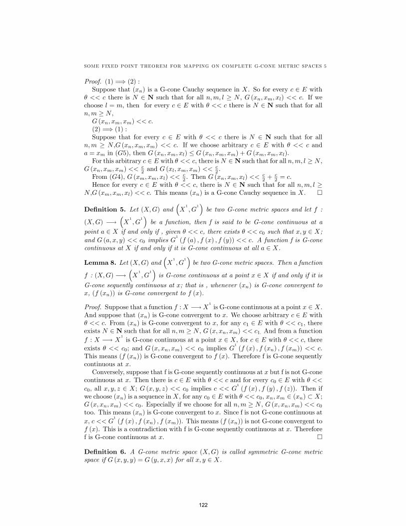
SOME FIXED POINT THEOREM FOR MAPPING ON COMPLETE G-CONE METRIC SPACES 5
Proof. (1) =) (2) :Suppose that (xn) is a G-cone Cauchy sequence in X. So for every c 2 E with
<< c there is N 2 N such that for all n;m; l N , G (xn; xm; xl) << c. If wechoose l = m, then for every c 2 E with << c there is N 2 N such that for alln;m N ,G (xn; xm; xm) << c.(2) =) (1) :Suppose that for every c 2 E with << c there is N 2 N such that for all
n;m N ,G (xn; xm; xm) << c. If we choose arbitrary c 2 E with << c anda = xm in (G5), then G (xn; xm; xl) G (xn; xm; xm) +G (xm; xm; xl).For this arbitrary c 2 E with << c, there isN 2 N such that for all n;m; l N ,
G (xn; xm; xm) <<c2 and G (xl; xm; xm) <<
c2 .
From (G4), G (xm; xm; xl) << c2 . Then G (xn; xm; xl) <<
c2 +
c2 = c.
Hence for every c 2 E with << c, there is N 2 N such that for all n;m; l N ,G (xm; xm; xl) << c. This means (xn) is a G-cone Cauchy sequence in X.
Denition 5. Let (X;G) andX
1
; G1be two G-cone metric spaces and let f :
(X;G) !X
1
; G1be a function, then f is said to be G-cone continuous at a
point a 2 X if and only if , given << c, there exists << c0 such that x; y 2 X;and G (a; x; y) << c0 implies G
1
(f (a) ; f (x) ; f (y)) << c. A function f is G-conecontinuous at X if and only if it is G-cone continuous at all a 2 X.
Lemma 8. Let (X;G) andX
1
; G1be two G-cone metric spaces. Then a function
f : (X;G) !X
1
; G1is G-cone continuous at a point x 2 X if and only if it is
G-cone sequently continuous at x; that is , whenever (xn) is G-cone convergent tox, (f (xn)) is G-cone convergent to f (x).
Proof. Suppose that a function f :X !X1
is G-cone continuous at a point x 2 X.And suppose that (xn) is G-cone convergent to x. We choose arbitrary c 2 E with << c. From (xn) is G-cone convergent to x, for any c1 2 E with << c1, thereexists N 2 N such that for all n;m N , G (x; xn; xm) << c1. And from a functionf : X ! X
1
is G-cone continuous at a point x 2 X, for c 2 E with << c, thereexists << c0; and G (x; xn; xm) << c0 implies G
1
(f (x) ; f (xn) ; f (xm)) << c.This means (f (xn)) is G-cone convergent to f (x). Therefore f is G-cone sequentlycontinuous at x.Conversely, suppose that f is G-cone sequently continuous at x but f is not G-cone
continuous at x. Then there is c 2 E with << c and for every c0 2 E with <<c0, all x; y; z 2 X; G (x; y; z) << c0 implies c << G
1
(f (x) ; f (y) ; f (z)). Then ifwe choose (xn) is a sequence inX, for any c0 2 E with << c0, xn; xm 2 (xn) X;G (x; xn; xm) << c0. Especially if we choose for all n;m N , G (x; xn; xm) << c0too. This means (xn) is G-cone convergent to x. Since f is not G-cone continuous atx, c << G
1
(f (x) ; f (xn) ; f (xm)). This means (f (xn)) is not G-cone convergent tof (x). This is a contradiction with f is G-cone sequently continuous at x. Thereforef is G-cone continuous at x.
Denition 6. A G-cone metric space (X;G) is called symmetric G-cone metricspace if G (x; y; y) = G (y; x; x) for all x; y 2 X.
122

6 DURAN TURKOGLU AND NURCAN BILGILI
Lemma 9. Let (X;G) be a G-cone metric space, P be a normal cone with normalconstant K. Then the function G (x; y; z) is jointly continuous in all three of itsvariables.
Proof. From Lemma 8, be G-cone continuous and be G-cone sequently continuousare equivalent in G-cone metric spaces. Hence, if G is jointly sequently continuousin all three of its variables, it is jointly continuous in all three of its variables.Suppose that (xn),(yn),(zn) are sequences in X and (xn) is G-cone convergent tox in X, (yn) is G-cone convergent to y in X, (zn) is G-cone convergent to z in X.For every " > 0, choose c 2 E with << c and kck < "
6K+3 . From (xn) is G-coneconvergent to x, (yn) is G-cone convergent to y, (zn) is G-cone convergent to z,there is N 2 N such that for all n;m N , G (x; xn; xm) << c, G (y; yn; ym) << c,G (z; zn; zm) << c. We have
G (x; y; z) G (x; xn; xn) +G (xn; y; z)
= G (x; xn; xn) +G (y; xn; z)
G (x; xn; xn) +G (y; yn; yn) +G (yn; xn; z)
= G (x; xn; xn) +G (y; yn; yn) +G (z; yn; xn)
G (x; xn; xn) +G (y; yn; yn) +G (z; zn; zn) +G (zn; yn; xn)
= G (x; xn; xn) +G (y; yn; yn) +G (z; zn; zn) +G (xn; yn; zn)
Hence G (x; y; z) G (x; xn; xn)+G (y; yn; yn)+G (z; zn; zn)+G (xn; yn; zn). Andsimilarly we have G (xn; yn; zn) G (xn; x; x)+G (yn; y; y)+G (zn; z; z)+G (x; y; z).From (G3),G (xn; x; x) = G (x; x; xn) G (x; xn; xm) << c and G (x; xn; xn) =G (xn; xn; x) G (xn; x; xm) = G (x; xn; xm) << c.Then
G (x; xn; xn) < < c and G (xn; x; x) << c;
G (y; yn; yn) < < c and G (yn; y; y) << c;
G (z; zn; zn) < < c and G (zn; z; z) << c:
Hence G (x; y; z) 3c+G (xn; yn; zn) and G (xn; yn; zn) 3c+G (x; y; z). Then
G (xn; yn; zn) + 3cG (x; y; z) 3c+G (x; y; z) + 3cG (x; y; z) = 6c:
Since P is a normal cone with normal constant K,
kG (xn; yn; zn)G (x; y; z)k kG (xn; yn; zn)G (x; y; z) + 3c 3ck kG (xn; yn; zn)G (x; y; z) + 3ck+ k3ck 6K kck+ 3 kck = (6K + 3) kck < ":
Therefore G (xn; yn; zn) ! G (x; y; z) (n !1).
Lemma 10. Every G-cone metric space (X;G) will dene a cone metric space(X; dG) by
(2.1) dG (x; y) = G (x; y; y) +G (y; x; x) ;8x; y 2 X
Note that if (X;G) is symmetric G-cone metric space, then
(2.2) dG (x; y) = 2G (x; y; y) ;8x; y 2 X
123

SOME FIXED POINT THEOREM FOR MAPPING ON COMPLETE G-CONE METRIC SPACES 7
However, if (X;G) is not symmetric, then it holds by the G-cone metric propertiesthat
(2.3)3
2G (x; y; y) dG (x; y) 3G (x; y; y) ;8x; y 2 X
and that in general these inequalities cannot be improved.
Proof. Suppose that (X;G) is G-cone metric space. And we choose dG (x; y) =G (x; y; y) +G (y; y; x), 8x; y 2 X. If dG (x; y) satises(d1) ; (d2),(d3), then it is a cone metric.(d1) For all x; y 2 X with x 6= y, dG (x; y) = G (x; y; y)+G (y; x; x). From (G2),
< G (x; y; y) and < G (y; x; x); for all x; y 2 X with x 6= y. Therefore <dG (x; y); for all x; y 2 X with x 6= y.From (G1),G (x; y; y) = and G (y; x; x) = if and only if x = y. Hence
dG (x; y) = if and only if x = y.(d2) For all x; y 2 X, dG (x; y) = G (x; y; y)+G (y; x; x) = G (y; x; x)+G (x; y; y) =
dG (y; x). Hence for all x; y 2 X, dG (x; y) = dG (y; x).(d3) For all x; y; z 2 X,
dG (x; y) = G (x; y; y) +G (y; x; x)
G (x; z; z) +G (z; y; y) +G (y; z; z) +G (z; x; x)
= G (x; z; z) +G (z; x; x) +G (z; y; y) +G (y; z; z)
= dG (x; z) + dG (z; y) :
From (d1), (d2) and (d3), dG (x; y) is a cone metric and (X; dG) is a cone metricspace.Now suppose that (X;G) is a symmetric G-cone metric space. Then for all
x; y 2 X,dG (x; y) = G (x; y; y) +G (y; x; x) = 2G (x; y; y).And suppose that if (X;G) is not symmetric, for all x; y 2 X, 3G (x; y; y) <
dG (x; y) <32G (x; y; y).
Then 6G (x; y; y) < 2dG (x; y) < 3G (x; y; y) hence from
2dG (x; y) < 3G (x; y; y) ;
2 [G (x; y; y) +G (y; x; x)] < 3G (x; y; y) ;
2G (y; x; x) < G (x; y; y) :
This is a contradiction, since, from (G5), for all x; y 2 X, G (x; y; y) = G (y; x; y) G (y; x; x) +G (x; x; y) = 2G (y; x; x).Similarly from
6G (x; y; y) < 2dG (x; y) ;
6G (x; y; y) < 2 [G (x; y; y) +G (y; x; x)] ;
4G (x; y; y) < 2G (y; x; x) ;
2G (x; y; y) < G (y; x; x) :
This is a contradiction too, since, from (G5), for all x; y 2 X,G (y; x; x) = G (x; y; x) G (x; y; y) +G (y; y; x) = 2G (x; y; y).These contradictions imply that for all x; y 2 X, 3
2G (x; y; y) dG (x; y) 3G (x; y; y).
124
8 DURAN TURKOGLU AND NURCAN BILGILI
Denition 7. A G-cone metric space (X;G) is G-cone complete (or complete G-cone) metric space if every G-cone Cauchy sequence in (X;G) is G-cone convergentin (X;G).
Lemma 11. A G-cone metric space (X;G) is complete G-cone metric space if andonly if (X; dG) is complete cone metric space.
Proof. Suppose that (X;G) is complete G-cone metric space and (xn) is a Cauchysequence in (X; dG). We choose arbitrary c 2 E with << c. From (xn) is a Cauchysequence in (X; dG), there is N 2 N such that for all n;m N , dG (xn; xm) << c
2 .Then dG (xn; xm) = G (xn; xm; xm) +G (xm; xn; xn) << c
2 .Hence for all n;m; l N , G (xn; xm; xl) G (xn; xm; xm) + G (xm; xm; xl) <<
c2 +
c2 = c.
This means (xn) is a G-cone Cauchy sequence in (X;G).Since (X;G) is completeG-cone metric space, (xn) is G-cone convergent to x in (X;G). Then for any c 2 Ewith << c, there is N1 2 N such that for all n;m N1,G (xn; xm; x) << c
2 .Hence from Lemma 3 for any c 2 E with << c, there is N1 2 N such that for alln N1,dG (xn; x) = G (xn; x; x) +G (x; xn; xn) << c
2 +c2 = c. This means (xn) is
convergent to x in (X; dG). Therefore (X; dG) is complete cone metric space.Conversely suppose that (X; dG) is complete cone metric space and (xn) is a
G-cone Cauchy sequence in (X;G). We choose arbitrary c 2 E with << c. From(xn) is a G-cone Cauchy sequence in (X;G), there is N 2 N such that for alln;m; l N , G (xn; xm; xl) << c
2 . Hence for all n;m = l N , dG (xn; xm) =G (xn; xm; xm) +G (xm; xn; xn) <<
c2 +
c2 = c.
This means (xn) is a Cauchy sequence in (X; dG). Since (X; dG) is completecone metric space, (xn) is convergent to x in (X; dG).Then for any c 2 E with << c, there is N1 2 N such that for all n N1,
dG (xn; x) <<c2 . Then dG (xn; x) = G (xn; x; x) +G (x; xn; xn) <<
c2 .
Hence from (G5), for any c 2 E with << c, there is N1 2 N such that for alln;m N1,G (xn; xm; x) G (xn; xm; xm) +G (xm; xm; x) G (xn; x; x) +G (x; xm; xm) +
G (xm; xm; x) <<c2 +
c2 = c.
This means (xn) is G-cone convergent to x in (X;G). Therefore (X;G) is com-plete G-cone metric space.
3. Main resultsHere we start our work with the following theorem.
Theorem 1. Let (X;G) be a complete G-cone metric space, P be a normal conewith normal constant K and let T : X ! X be a mapping satisfying one of thefollowing conditions
G (T (x) ; T (y) ; T (z)) faG (x; y; z) + bG (x; T (x) ; T (x))+cG (y; T (y) ; T (y)) + dG (z; T (z) ; T (z))g(3.1)
or
G (T (x) ; T (y) ; T (z)) faG (x; y; z) + bG (x; x; T (x))+cG (y; y; T (y)) + dG (z; z; T (z))g(3.2)
for all x; y; z 2 X where 0 a+ b+ c+ d < 1, then T has a unique xed point (sayu, i.e., Tu = u), and T is G-cone continuous at u.
125
SOME FIXED POINT THEOREM FOR MAPPING ON COMPLETE G-CONE METRIC SPACES 9
Proof. Suppose that T satises condition (3.1), then for all x; y 2 X, we haveG (Tx; Ty; Ty) aG (x; y; y) + bG (x; Tx; Tx) + (c+ d)G (y; Ty; Ty) ;
(3.3)
G (Ty; Tx; Tx) aG (y; x; x) + bG (y; Ty; Ty) + (c+ d)G (x; Tx; Tx)Suppose that (X;G) is symmetric, then by denition of cone metric (X; dG) and
( 2.2), we get for all x; y 2 X;
dG (Tx; Ty) adG (x; y) +c+ d+ b
2dG (x; Tx)
+c+ d+ b
2dG (y; Ty)(3.4)
In this line, since 0 a + b + c + d < 1, then the existence and uniqueness of thexed point follows from well-known theorem in cone metric space (X; dG).(see [9])However, if (X;G) is not symmetric then by denition of cone metric (X; dG)
and (2.3), we get for all x; y 2 X:
dG (Tx; Ty) adG (x; y) +2 (c+ d+ b)
3dG (x; Tx)
+2 (c+ d+ b)
3dG (y; Ty)(3.5)
Then the cone metric condition gives no information about this map since 0 <a+ 2(c+d+b)
3 + 2(c+d+b)3 need not be less than 1. But this can be proved by G-cone
metric.Let x0 2 X be an arbitrary point, and dene the sequence (xn) by xn = Tn (x0).
By (3.1), we have
G (xn; xn+1; xn+1) aG (xn1; xn; xn) + bG (xn1; xn; xn)
+ (c+ d)G (xn; xn+1; xn+1) ;(3.6)
then
(3.7) G (xn; xn+1; xn+1) a+ b
1 (c+ d)G (xn1; xn; xn) :
Let q = a+b1(c+d) , then 0 q < 1 since 0 a+ b+ c+ d < 1. So,
(3.8) G (xn; xn+1; xn+1) qG (xn1; xn; xn) :Continuing in the same argument, we will get
(3.9) G (xn; xn+1; xn+1) qnG (x0; x1; x1) :Moreover, for all n;m 2 N; n < m, we have by rectangle inequality
G (xn; xm; xm) G (xn; xn+1; xn+1) +G (xn+1; xn+2; xn+2)
+G (xn+2; xn+3; xn+3) + :::+G (xm1; xm; xm)
qn + qn+1 + :::+ qm1
G (x0; x1; x1)
qn
1 qG (x0; x1; x1) ;(3.10)
Since P is a normal cone with normal constant K,
kG (xn; xm; xm)k Kqn
1 q kG (x0; x1; x1)k :
126
10 DURAN TURKOGLU AND NURCAN BILGILI
This means limG (xn; xm; xm) = , as n;m ! 1. Thus, from Lemma 7, (xn) isG-cone Cauchy sequence. Due to the completeness of (X;G), there exists u 2 Xsuch that (xn) is G-cone converge to u.Suppose that Tu 6= u, then
G (xn; T (u) ; T (u)) aG (xn1; u; u) + bG (xn1; xn; xn)
+ (c+ d)G (u; T (u) ; T (u)) ;(3.11)
Since P is a normal cone with normal constant K,
kG (xn; T (u) ; T (u))k K (a kG (xn1; u; u)k+ b kG (xn1; xn; xn)k+(c+ d) kG (u; T (u) ; T (u))k :)
And using the fact that (xn) is G-cone Cauchy sequence, (xn) is G-cone convergeto u, then
kG (xn; T (u) ; T (u))k (c+ d) kG (u; T (u) ; T (u))k :This contradiction implies that u = Tu. To prove uniqueness, suppose that u 6= vsuch that Tv = v, then
G (u; v; v) aG (u; v; v) + bG (u; T (u) ; T (u))
+ (c+ d)G (v; T (v) ; T (v))
= aG (u; v; v)(3.12)
Since P is a normal cone with normal constant K,kG (u; v; v)k Ka kG (u; v; v)k :This contradiction implies that u = v. To show that T is G-cone continuous at u,let (yn) X be a sequence such that lim
n!1(yn) = u. We can deduce that
G (u; T (yn) ; T (yn)) aG (u; yn; yn) + bG (u; T (u) ; T (u))
+ (c+ d)G (yn; T (yn) ; T (yn))
= aG (u; yn; yn) + (c+ d)G (yn; T (yn) ; T (yn)) ;(3.13)
and since G (yn; T (yn) ; T (yn)) G (yn; u; u) +G (u; T (yn) ; T (yn)), we have that
G (u; T (yn) ; T (yn)) a
1 (c+ d)G (u; yn; yn)
+c+ d
1 (c+ d)G (yn; u; u) :
Since P is a normal cone with normal constant K,
kG (u; T (yn) ; T (yn))k K
a
1 (c+ d) kG (u; yn; yn)k
+c+ d
1 (c+ d) kG (yn; u; u)k:
Taking the limit as n ! 1, from which we see that G (u; T (yn) ; T (yn)) ! and so, by Lemma 8, T (yn) ! u = Tu. It is proved that T is G-cone continuousat u.If T satises condition (3.2), then the argument is similar to that above. However,
to show that the sequence (xn) is G-cone Cauchy, we start with
G (xn; xn; xn+1) aG (xn1; xn1; xn) + (b+ c)G (xn1; xn1; xn)
+dG (xn; xn; xn+1) ;(3.14)
127
SOME FIXED POINT THEOREM FOR MAPPING ON COMPLETE G-CONE METRIC SPACES11
then
(3.15) G (xn; xn; xn+1) a+ b+ c
1 d G (xn1; xn1; xn) :
Let q = a+b+c1d , then 0 q < 1 since 0 a+ b+ c+ d < 1.
Continuing in the same way, we nd that
(3.16) G (xn; xn; xn+1) qnG (x0; x0; x1) :Then for all n;m 2 N; n < m, we have by repeated use of the rectangle inequalityG (xn; xn; xm) qn
1qG (x0; x0; x1) :
Corollary 1. Let (X;G) be a complete G-cone metric space, P be a normal conewith normal constant K and let T : X ! X be a mapping satisfying one of thefollowing conditions:
G (Tm (x) ; Tm (y) ; Tm (z)) faG (x; y; z) + bG (x; Tm (x) ; Tm (x))+cG (y; Tm (y) ; Tm (y)) + dG (z; Tm (z) ; Tm (z))g(3.17)
or
G (Tm (x) ; Tm (y) ; Tm (z)) faG (x; y; z) + bG (x; x; Tm (x))+cG (y; y; Tm (y)) + dG (z; z; Tm (z))g ;(3.18)
for all x; y; z 2 X, where 0 a + b + c + d < 1. Then T has a unique xed point(say u), and Tm is G-cone continuous at u.
Proof. From the previous theorem, we see that Tm has a unique xed point (sayu), that is, Tm (u) = u. But T (u) = T (Tm (u)) = Tm+1 (u) = Tm (T (u)), so T (u)is another xed point for Tm and by uniqueness Tu = u. Theorem 2. Let (X;G) be a complete G-cone metric space, P be a normal conewith normal constant K and let T : X ! X be a mapping. If for some constant0 k < 1 and for all x; y; z 2 X, there exists
u 2 fG (x; T (x) ; T (x)) ; G (y; T (y) ; T (y)) ; G (z; T (z) ; T (z))gsuch that
(3.19) G (T (x) ; T (y) ; T (z)) kuor there exists
w 2 fG (x; x; T (x)) ; G (y; y; T (y)) ; G (z; z; T (z))gsuch that
(3.20) G (T (x) ; T (y) ; T (z)) kw;then T has a unique xed point (say u), and T is G-cone continuous at u.
Proof. Suppose that T satises condition (3.19), then for some constant 0 k < 1and for all x; y 2 X, there exists
u 2 fG (x; Tx; Tx) ; G (y; Ty; Ty)gsuch that
G (Tx; Ty; Ty) ku;
(3.21)
G (Ty; Tx; Tx) ku:
128
12 DURAN TURKOGLU AND NURCAN BILGILI
Suppose that (X;G) is symmetric, then by denition of the cone metric (X; dG)and (2.2), there exists v = 2u 2 fdG (x; Tx) ; dG (y; Ty)g such that dG (Tx; Ty) kv;8x; y 2 X: Since 0 k < 1, then the existence and uniqueness of the xed pointfollows from a theorem in cone metric space (X; dG). (see [9])However, if (X;G) is not symmetric, then by denition of the metric (X; dG)
and (2.3), there exists v 2 fdG (x; Tx) ; dG (y; Ty)g such that
(3.22) dG (Tx; Ty) 4k
3v;8x; y 2 X:
The cone metric condition gives no information about this map since 4k3 need not
be less than 1, but we will proof it by G-cone metric. Let x0 2 X be an arbitrarypoint, and dene the sequence (xn) by xn = Tn (x0). By (3.19), there existsu 2 fG (xn1; xn; xn) ; G (xn; xn+1; xn+1)g such that
G (xn; xn+1; xn+1) ku
= k (Gxn1; xn; xn) (since 0 k < 1) .(3.23)
Continuing in the same argument, we will nd
(3.24) G (xn; xn+1; xn+1) knG (x0; x1; x1) :For all n;m 2 N; n < m, we have by rectangle inequality that
G (xn; xm; xm) G (xn; xn+1; xn+1) +G (xn+1; xn+2; xn+2)
+G (xn+2; xn+3; xn+3) + :::+G (xm1; xm; xm)
kn + kn+1 + :::+ km1
G (x0; x1; x1)
kn
1 kG (x0; x1; x1) :(3.25)
Since P is a normal cone with normal constant K,
kG (xn; xm; xm)k Kkn
1 k kG (x0; x1; x1)k :
Then, limG (xn; xm; xm) = , as n;m ! 1, and thus, from Lemma 7, (xn) isG-cone Cauchy sequence. Due to the completeness of (X;G), there exists u 2 Xsuch that (xn) ! u.Suppose that Tu 6= u, then there exists
t 2 fG (xn+1; xn+2; xn+2) ; G (u; T (u) ; T (u))gsuch that G (xn+1; T (u) ; T (u)) kt. Since P is a normal cone with normal con-stant K,
kG (xn+1; T (u) ; T (u))k Kk ktkand by taking the limit as n ! 1, and using the fact that (xn) is G-coneCauchy sequence, (xn) is G-cone converge to u, we get that kG (u; T (u) ; T (u))k Kk kk = 0 or kG (u; T (u) ; T (u))k Kk kG (u; T (u) ; T (u))k : Then these impliethat u = Tu.To prove uniqueness, suppose that u 6= v such that Tv = v, then there exists
p 2 fG (v; v; v) ; G (u; u; u)g such that G (u; v; v) kp = which implies that u = v.To show that T is G-cone continuous at u, let (yn) X be a sequence such thatlim
n!1(yn) = u, then there exists q 2 fG (u; T (u) ; T (u)) ; G (yn; T (yn) ; T (yn))g
such that
(3.26) G (u; T (yn) ; T (yn)) kq:
129
SOME FIXED POINT THEOREM FOR MAPPING ON COMPLETE G-CONE METRIC SPACES13
Then G (u; T (yn) ; T (yn)) kG (u; T (u) ; T (u)) = implies that T (yn) = u,8n 2 N. Or G (u; T (yn) ; T (yn)) kG (yn; T (yn) ; T (yn)) :But,
G (yn; T (yn) ; T (yn)) G (yn; u; u) +G (u; T (yn) ; T (yn))
then G (u; T (yn) ; T (yn))
k1k
G (yn; u; u) : Since P is a normal cone with
normal constant K, kG (u; T (yn) ; T (yn))k K
k1k
kG (yn; u; u)k : Taking the
limit as n ! 1, from which we see that G (u; T (yn) ; T (yn)) ! , and so byLemma 8, T (yn) ! u = Tu. So these implie that T is G-cone continuous atu. Corollary 2. Let (X;G) be a complete G-cone metric space, P be a normal conewith normal constant K and let T : X ! X be a mapping. If for some m 2 N,some constant 0 k < 1 and for all x; y; z 2 X, there exists
u 2 fG (x; Tm (x) ; Tm (x)) ; G (y; Tm (y) ; Tm (y)) ; G (z; Tm (z) ; Tm (z))gsuch that
(3.27) G (Tm (x) ; Tm (y) ; Tm (z)) kuor there exists
w 2 fG (x; x; Tm (x)) ; G (y; y; Tm (y)) ; G (z; z; Tm (z))gsuch that
(3.28) G (Tm (x) ; Tm (y) ; Tm (z)) kw;then T has a unique xed point (say u), and Tm is G-cone continuous at u.
Proof. We use the same argument as in Corollary 1. Theorem 3. Let (X;G) be a complete G-cone metric space, P be a normal conewith normal constant K and let T : X ! X be a mapping. If for some constant0 k < 1 and for all x; y 2 X, there exists
u 2 fG (x; T (y) ; T (y)) ; G (y; T (x) ; T (x)) ; G (y; T (y) ; T (y))gsuch that
(3.29) G (T (x) ; T (y) ; T (y)) kuor there exists
w 2 fG (x; x; T (y)) ; G (y; y; T (x)) ; G (y; y; T (y))gsuch that
(3.30) G (T (x) ; T (y) ; T (y)) kw;then T has a unique xed point (say u) and T is G-cone continuous at u.
Proof. Suppose that T satises condition (3.29) then for some constant 0 k < 1and for all x; y 2 X, there exists
u1 2 fG (x; Ty; Ty) ; G (y; Tx; Tx) ; G (y; Ty; Ty)g ;u2 2 fG (x; Ty; Ty) ; G (y; Tx; Tx) ; G (x; Tx; Tx)g
such thatG (Tx; Ty; Ty) ku1;
(3.31)
130

14 DURAN TURKOGLU AND NURCAN BILGILI
G (Ty; Tx; Tx) ku2:Suppose that (X;G) is symmetric, then by denition of the cone metric (X; dG)and (2.2), there exists
v 2dG (x; Ty) ; dG (y; Tx) ;
1
2dG (x; Tx) ;
1
2dG (y; Ty)
such that
(3.32) dG (Tx; Ty) kv;8x; y 2 XSince 0 k < 1, then the existence and uniqueness of the xed point follows froma theorem in cone metric space (X; dG). However, if (X;G) is not symmetric, thenby denition of the metric (X; dG) and (2.3), there exists
v 2dG (x; Ty) ; dG (y; Tx) ;
1
2dG (x; Tx) ;
1
2dG (y; Ty)
such that
(3.33) dG (Tx; Ty) 4k
3v;8x; y 2 X:
The cone metric condition gives no information about this map since 4k3 need not
be less than 1, but we will proof it by G-cone metric. Let x0 2 X be an arbitrarypoint, and dene the sequence (xn) by xn = Tn (x0). By 3.29, there exists
u3 2 fG (xn1; xn+1; xn+1) ; G (xn; xn+1; xn+1)gsuch that
G (xn; xn+1; xn+1) ku3
= kG (xn1; xn+1; xn+1) (since 0 k < 1):(3.34)
So,
(3.35) G (xn; xn+1; xn+1) kG (xn1; xn+1; xn+1) ;and using there exists
u4 2 fG (xn2; xn+1; xn+1) ; G (xn; xn1; xn1) ; G (xn; xn+1; xn+1)gsuch that
(3.36) G (xn1; xn+1; xn+1) ku4;then,
(3.37) G (xn; xn+1; xn+1) k2u4:Continuing in this procedure, we will have
(3.38) G (xn; xn+1; xn+1) knTn;where
Tn 2 fG (xi; xj ; xj) ; for all i; j 2 f0; 1; :::; n+ 1gg :Then for all n;m 2 N; n < m, we have by rectangle inequality
G (xn; xm; xm) G (xn; xn+1; xn+1) +G (xn+1; xn+2; xn+2)
+G (xn+2; xn+3; xn+3) + :::+G (xm1; xm; xm)
knTn + kn+1Tn+1 + :::+ k
m1Tm1(3.39)
131
SOME FIXED POINT THEOREM FOR MAPPING ON COMPLETE G-CONE METRIC SPACES15
Since P is a normal cone with normal constant K,
kG (xn; xm; xm)k K knTn + kn+1Tn+1 + :::+ km1Tm1
Kkn kTnk+ kn+1 kTn+1k+ :::+ km1 kTm1k
;
If we choose T0 = max fkTik ; for all i = n; :::;m 1g thenkG (xn; xm; xm)k K
kn + kn+1 + :::+ km1
T0
Kkn
1 kT0:
Then, limG (xn; xm; xm) = , as n;m !1, and thus, from Lemma (1.11), (xn) isG-cone Cauchy sequence. Since (X;G) is G-cone complete then there exists u 2 Xsuch that (xn) is G-cone converge to u. Suppose that Tu 6= u, then by (3.29), thereexists
t 2 fG (xn1; T (u) ; T (u)) ; G (u; xn+1; xn+1) ; G (u; T (u) ; T (u))gsuch that
(3.40) G (xn; T (u) ; T (u)) kt:Taking the limit as n !1, we get G (u; T (u) ; T (u)) = implies Tu = u or
G (u; T (u) ; T (u)) kG (u; T (u) ; T (u)), this contradiction implies that u = Tu. To prove the uniqueness, suppose thatu 6= v such that Tv = v. So, by (3.29), there exists t 2 fG (u; v; v) ; G (v; u; u)gsuch that
(3.41) G (u; v; v) kt) G (u; v; v) kG (v; u; u) :Again we will nd G (v; u; u) kG (u; v; v), so(3.42) G (u; v; v) k2G (u; v; v) ;since P is a normal cone with normal constant K,
kG (u; v; v)k Kk2 kG (u; v; v)k, since 0 k < 1, this implies that u = v. To show that T is G-cone continuousat u, let (yn) X be a sequence such that lim
n!1(yn) = u, then by (3.29), there
exists
t 2 fG (u; T (yn) ; T (yn)) ; G (yn; T (u) ; T (u)) ; G (yn; T (yn)T (yn))gsuch that
(3.43) G (u; T (yn) ; T (yn)) kt:But,
G (yn; T (yn) ; T (yn)) G (yn; u; u) +G (u; T (yn)T (yn))so, G (u; T (yn) ; T (yn)) k
1kG (yn; u; u).Since P is a normal cone with normal constant K,
kG (u; T (yn) ; T (yn))k Kk
1 k kG (yn; u; u)k :
Taking the limit as n !1, from which we see that G (u; T (yn) ; T (yn)) ! and so, by Lemma (1.13), we have T (yn) ! u = Tu which implies that T isG-cone continuous at u.
132
16 DURAN TURKOGLU AND NURCAN BILGILI
Corollary 3. Let (X;G) be a complete G-cone metric space, P be a normal conewith normal constant K and let T : X ! X be a mapping. If for some constant0 k < 1 and for all x; y; z 2 X, there exists
u 2
8<: G (x; T (y) ; T (y)) ; G (x; T (z) ; T (z)) ;G (y; T (x) ; T (x)) ; G (y; T (z) ; T (z)) ;G (z; T (x) ; T (x)) ; G (z; T (y) ; T (y))
9=;such that
(3.44) G (T (x) ; T (y) ; T (z)) ku;there exists
w 2
8<: G (x; x; T (y)) ; G (x; x; T (z)) ;G (y; y; T (x)) ; G (y; y; T (z)) ;G (z; z; T (x)) ; G (z; z; T (y))
9=;such that
(3.45) G (T (x) ; T (y) ; T (z)) kw:Then T has a unique xed point (say u) and T is G-cone continuous at u.
Proof. If we let z = y in conditions (3.44) and (3.45), then they become conditions(3.29) and (3.30), respectively, in Theorem 3; so the proof follows from Theorem3.
Corollary 4. Let (X;G) be a complete G-cone metric space, P be a normal conewith normal constant K and let T : X ! X be a mapping. If for some m 2 N,some constant 0 k < 1 and for all x; y; z 2 X, there exists
u 2
8<: G (x; Tm (y) ; Tm (y)) ; G (x; Tm (z) ; Tm (z)) ;G (y; Tm (x) ; Tm (x)) ; G (y; Tm (z) ; Tm (z)) ;G (z; Tm (x) ; Tm (x)) ; G (z; Tm (y) ; Tm (y))
9=; ;w 2
8<: G (x; x; Tm (y)) ; G (x; x; Tm (z)) ;G (y; y; Tm (x)) ; G (y; y; Tm (z)) ;G (z; z; Tm (x)) ; G (z; z; Tm (y))
9=;, t1 2 fG (x; Tm (y) ; Tm (y)) ; G (y; Tm (x) ; Tm (x)) ; G (y; Tm (y) ; Tm (y))g suchthat
G (Tm (x) ; Tm (y) ; Tm (z)) ku;
G (Tm (x) ; Tm (y) ; Tm (z)) kw;(3.46)
G (Tm (x) ; Tm (y) ; Tm (y)) kt1:
or t2 2 fG (x; x; Tm (y)) ; G (y; y; Tm (x)) ; G (y; y; Tm (y))g such that(3.47) G (Tm (x) ; Tm (y) ; Tm (y)) kt2:Then T has a unique xed point (say u) and Tm is G-cone continuous at u.
Proof. The proof follows from Theorem 3, Corollary 3, and from an argumentsimilar to that used in Corollary 1.
Theorem 4. Let (X;G) be a complete G-cone metric space, P be a normal conewith normal constant K and let T : X ! X be a mapping. If for some constant0 k < 1 and for all x; y 2 X, there exists
u 2 fG (x; T (y) ; T (y)) ; G (y; T (x) ; T (x))g
133

SOME FIXED POINT THEOREM FOR MAPPING ON COMPLETE G-CONE METRIC SPACES17
such that
(3.48) G (T (x) ; T (y) ; T (y)) kuor there exists
w 2 fG (x; x; T (y)) ; G (y; y; T (x))gsuch that
(3.49) G (T (x) ; T (y) ; T (y)) kw;then T has a unique xed point (say u) and T is G-cone continuous at u.
Proof. Since whenever the mapping satises condition (3.48), or (3.49), then itsatises condition (3.44), or (3.45), respectively, in Theorem 3. Then the prooffollows from Theorem 3. Corollary 5. Let (X;G) be a complete G-cone metric space, P be a normal conewith normal constant K and let T : X ! X be a mapping satisfying one of thefollowing conditions :
(3.50) G (T (x) ; T (y) ; T (y)) a fG (x; T (y) ; T (y)) +G (y; T (x) ; T (x))gor
(3.51) G (T (x) ; T (y) ; T (y)) a fG (x; x; T (y)) +G (y; y; T (x))gfor all x; y 2 X, where a 2
0; 12
, then T has a unique xed point (say u,i.e.,Tu =
u), and T is G-cone continuous at u.
Proof. Suppose that T satises condition (3.50), then we have
G (Tx; Ty; Ty) a fG (y; Tx; Tx) +G (x; Ty; Ty)g ;
(3.52)
G (Ty; Tx; Tx) a fG (x; Ty; Ty) +G (y; Tx; Tx)g ;for all x; y 2 X.Suppose that (X;G) is symmetric, then by denition of the cone metric (X; dG)
and (2.2), we get
(3.53) dG (Tx; Ty) a fdG (x; Ty) + dG (y; Tx)g ;8x; y 2 X:Since 0 2a < 1, then the existence and uniqueness of the xed point follow froma theorem in cone metric space (X; dG).However, if (X;G) is not symmetric, then by denition of the metric (X; dG)
and (2.3), we have
(3.54) dG (Tx; Ty) 4a
3dG (x; Ty) +
4a
3dG (y; Tx) ;8x; y 2 X:
So, the cone metric space (X; dG) gives no information about this map since 8a3
need not be less than 1. But this can be proved by G-cone metric.Let x0 2 X be arbitrary point, and dene the sequence (xn) by xn = Tn (x0),
then by (3.50), we have
G (xn; xn+1; xn+1) a fG (xn1; xn+1; xn+1) +G (xn; xn; xn)g= aG (xn1; xn+1; xn+1) :(3.55)
But
(3.56) G (xn1; xn+1; xn+1) aG (xn1; xn; xn) + aG (xn; xn+1; xn+1) ;
134
18 DURAN TURKOGLU AND NURCAN BILGILI
thus we have
(3.57) G (xn; xn+1; xn+1) a
1 aG (xn1; xn; xn) :
Let k = a1a , hence 0 k < 1 then continue in this procedure, we will get that
G (xn; xn+1; xn+1) knG (x0; x1; x1) :For all n;m 2 N; n < m, we have by rectangle inequality that
G (xn; xm; xm) G (xn; xn+1; xn+1) +G (xn+1; xn+2; xn+2)
+G (xn+2; xn+3; xn+3) + :::+G (xm1; xm; xm)
kn + kn+1 + :::+ km1
G (x0; x1; x1) :
kn
1 kG (x0; x1; x1) :(3.58)
Since P is a normal cone with normal constant K,
kG (xn; xm; xm)k Kkn
1 k kG (x0; x1; x1)k :
Then,limG (xn; xm; xm) = , as n;m ! 1, and thus, from Lemma (1.11), (xn)is G-cone Cauchy sequence. Due to the completeness of (X;G), there exists u 2 Xsuch that (xn) ! u.Suppose that Tu 6= u, then
G (xn; T (u) ; T (u)) a fG (xn1; T (u) ; T (u)) +G (u; xn; xn)g :Since P is a normal cone with normal constant K,
kG (xn; T (u) ; T (u))k Ka kG (xn1; T (u) ; T (u)) +G (u; xn; xn)kand by taking the limit as n !1, and using the fact that (xn) is G-cone Cauchysequence, (xn) is G-cone converge to u, we get that
kG (u; T (u) ; T (u))k Ka kG (u; T (u) ; T (u))k :This contradiction implies that u = Tu.To prove uniqueness, suppose that u 6= v such that Tv = v, then
G (u; v; v) a fG (u; v; v) +G (v; u; u)gso
(3.59) G (u; v; v) k =
a
1 a
G (v; u; u) ;
again by the same argument, we can verify that G (u; v; v) k2G (u; v; v), since Pis a normal cone with normal constant K,
kG (u; v; v)k Kk2 kG (u; v; v)k :This contradiction implies that u = v.To show that T is G-cone continuous at u, let (yn) X be a sequence such that
lim (yn) = u, then
(3.60) G (u; T (yn) ; T (yn)) a fG (u; T (yn) ; T (yn)) +G (yn; T (u) ; T (u))g ;and so
G (u; T (yn) ; T (yn))
a
1 a
G (yn; T (u) ; T (u)) :
135
SOME FIXED POINT THEOREM FOR MAPPING ON COMPLETE G-CONE METRIC SPACES19
Since P is a normal cone with normal constant K,
kG (u; T (yn) ; T (yn))k
a
1 a
kG (yn; T (u) ; T (u))k :
Taking the limit as n !1, from which we see that G (u; T (yn) ; T (yn)) ! . ByLemma (8), we have T (yn) ! u = Tu which implies that T is G-cone continuousat u.
Acknowledgement 1. The research has been supported by The Scientic andTechnological Research Council of Turkey (TUB·ITAK-Turkey).
References
[1] D. Ilic, V. Rakocevic, Common Fixed Points for Maps on Cone Metric Space. J. Math. Anal.Appl. (2007), doi:10.1016/j.jmaa. 2007.10.065.
[2] D. Turkoglu, M. Abuloha, Cone Metric Spaces and Fixed Point Theorems in DiametricallyContractive Mappings. Acta Mathematica Sinica, English Series (2010), doi:10.1007/s10114-010-8019-5.
[3] R. Raja, S. M. Vaezpour, Some Extensions of Banachs Contraction Principle inComplete Cone Metric Spaces. Fixed Point Theory and Applications, Vol. 2008, doi:10.1155/2008/768294.
[4] L.G. Huang, X. Zhang, Cone Metric Spaces and Fixed Point Theorems of Contractive Map-pings. J. Math. Anal. Appl., 332, 1468-1476, 2007.
[5] M. Abbas, G. Jungck, Common Fixed Point Results for Non Commuting Mappings With-out Continuity in Cone Metric Spaces. J. Math. Anal. Appl. (2007), doi: 10.10161/j.Jmaa.2007.09.070.
[6] Pasquale Vetro, Common Fixed Points in Cone Metric Spaces. Rendi Conti Del MatematicoDi Palermo. Serie II, Tomo LVI, 464-468,2007.
[7] Sh. Rezapour, R. Hamlbarani, Some Notes on the Paper "Cone Metric Spaces and FixedPoint Theorems of Contractive Mappings". J. Math. Anal. Appl. (2008),doi10.1016.
[8] D. Ilic, V. Rakocevic, Quasi-Contraction on Cone Metric space. Applied Mathematics Letters(2008), doi:10.1016/j.aml.2008.08/011.
[9] M. Abbas, B.E.Rhoades, Fixed and Periodic Point Results in Cone metric Spaces. AppliedMathematics Letters (2008), doi:10.1016/j.aml.2008.07/001.
[10] D. Wardowski, Endpoint and Fixed Points of set-valued Contractions in Cone Metric Spaces,Nonlinear Analysis (2008), doi:10.1016/j.na.2008.10.089.
[11] K. Deimling, Nonlinear Functional Analysis, Springer-Verlage, 1985.[12] Sh. Rezapour, Best Approximations in Cone Metric Spaces, Mathematica Moravica, Vol.11
(2007), 85-88.[13] Cristina Di Bari, Pasquale Vetro, 'Pairs and Common Fixed Points in Cone Metric Spaces,
Rendiconti del Circolo Matematico di Palermo, 57,doi: 10.1007/s 12215-008-0020-9, 2008.[14] S. Gahler, 2-metrische R¨ aume und ihre topologische Struktur, Mathematische
Nachrichten, vol. 26, pp. 115148, 1963.[15] S. Gahler, Zur geometric 2-metriche raume,Revue Roumaine de Math´ematiques Pures et
Appliqu´ees, vol. 40, pp. 664669, 1966.[16] K. S. Ha, Y. J. Cho, and A. White, Strictly convex and strictly 2-convex 2-normed spaces,
Mathematica Japonica, vol. 33, no. 3, pp. 375384, 1988.[17] B. C. Dhage, Generalized metric space and mapping with xed point, Bulletin of the
Calcutta Mathematical Society, vol. 84, pp. 329336, 1992.[18] B. C. Dhage, Generalized metric spaces and topological structure. I,Analele Stiintice ale
Universit¼atii Al. I. Cuza din Iasi. Serie Nou¼a. Matematic¼a, vol. 46, no. 1, pp. 324, 2000.[19] B. C. Dhage, On continuity of mappings in D-metric spaces, Bulletin of the Calcutta
Mathematical Society, vol. 86, no. 6, pp. 503508, 1994.[20] Z. Mustafa and B. Sims, Some remarks concerning D-metric spaces, International Confer-
ence on Fixed Point Theory and Applications, pp. 189198, Yokohama, Yokohama, Japan,2004.
136
20 DURAN TURKOGLU AND NURCAN BILGILI
[21] Zead Mustafa, Hamed Obiedat, and Fadi Awawdeh, Some Fixed Point Theorem for Mappingon Complete G-Metric Spaces,Fixed Point Theory and Applications, vol. 2008, Article ID189870, 12 pages, 2008. doi:10.1155/2008/189870
Department of Mathematics,Faculty of Science and Arts,Gazi University,Teknikokullar,06500,Ankara-Turkey
E-mail address : [email protected]
Department of Mathematics,Institute of Science and Technology,Gazi University,06500,Ankara-Turkey
E-mail address : [email protected]
137
Stability of an additive–quadratic functionalequation in menger probabilistic normed spaces
M. Eshaghi Gordji
Department of Mathematics, Semnan University, P. O. Box 35195-363,Semnan, Iran;
Center of Excellence in Nonlinear Analysis and Applications (CENAA),Semnan University, Semnan, Iran,e-mail: [email protected]
M. Bavand Savadkouhi
Department of Mathematics, Semnan University, P. O. Box 35195-363, Semnan, Iran;Center of Excellence in Nonlinear Analysis and Applications (CENAA), Semnan
University, Semnan, Iran,e-mail: [email protected]
S. M. Vaezpour
Department of Mathematics, Amir Kabir University, Tehran, Irane-mail: [email protected]
Abstract. In this paper, we establish the generalized Hyres–Ulam–Rassias stability of themixed type additive and quadratic functional equation
f(3x+ y) + f(3x− y) = f(x+ y) + f(x− y) + 2f(3x)− 2f(x)
in menger probabilistic normed spaces.
1. Introduction
The stability problem of functional equations originated from a question of Ulam [30] in 1940,concerning the stability of group homomorphisms. Let (G1, .) be a group and let (G2, ∗, d)be a metric group with the metric d(., .). Given ε > 0, does there exist a δ > 0, such that if amapping h : G1 → G2 satisfies the inequality d(h(x.y), h(x)∗h(y)) < δ for all x, y ∈ G1, thenthere exists a homomorphism H : G1 → G2 with d(h(x), H(x)) < ε for all x ∈ G1? In theother words, under what condition does there exist a homomorphism near an approximatehomomorphism? The concept of stability for functional equation arises when we replace thefunctional equation by an inequality which acts as a perturbation of the equation. In 1941,D. H. Hyers [16] gave a first affirmative answer to the question of Ulam for Banach spaces.Let f : E → E′ be a mapping between Banach spaces such that
‖f(x+ y)− f(x)− f(y)‖ ≤ δ
for all x, y ∈ E, and for some δ > 0. Then there exists a unique additive mapping T : E → E′
such that
‖f(x)− T (x)‖ ≤ δ
02000 Mathematics Subject Classification: 46S40,54E40.0Keywords: Stability; Additive functional equation; Quadratic functional equation;
menger probabilistic normed spaces.
138
JOURNAL OF APPLIED FUNCTIONAL ANALYSIS, VOL.7, NO’S 1-2,138-147,COPYRIGHT 2012 EUDOXUS PRESS,LLC

2 M. Eshaghi Gordji, M. B. Savadkouhi and S. M. Vaezpour
for all x ∈ E. Moreover if f(tx) is continuous in t ∈ R for each fixed x ∈ E, then T is linear.In 1978, Th. M. Rassias [26] provided a generalization of Hyers’ Theorem which allows theCauchy difference to be unbounded. In 1991, Z. Gajda [9] answered the question for thecase p > 1, which was rased by Rassias. This new concept is known as Hyers–Ulam–Rassiasstability of functional equations (see [1], [10, 15, 17] and [24, 25]). The functional equation
f(x+ y) + f(x− y) = 2f(x) + 2f(y). (1.1)
is related to symmetric bi–additive function. It is natural that this equation is called aquadratic functional equation. In particular, every solution of the quadratic equation (1.1)is said to be a quadratic function. It is well known that a function f between real vectorspaces is quadratic if and only if there exits a unique symmetric bi–additive function B suchthat f(x) = B(x, x) for all x (see [1, 18]). The bi–additive function B is given by
B(x, y) =1
4(f(x+ y)− f(x− y)) (1.2)
Hyers–Ulam–Rassias stability problem for the quadratic functional equation (1.1) was provedby Skof for functions f : A → B, where A is normed space and B Banach space [29] (seealso [2, 4] and [13]).We mention here the papers [7, 8, 11] and [12] concerning the stability of the mixed typefunctional equations.
The generalized Hyers–Ulam–Rassias stability of different functional equations in randomnormed and fuzzy normed spaces has been recently studied in [6], [19], [20], [21], [22] and[23]. It should be noticed that in all these papers the triangle inequality is expressed by usingthe strongest triangular norm TM . Throughout this paper, ∆+ is the space of distributionfunctions that is, the space of all mappings F : R ∪ −∞,∞ → [0, 1], such that F is left–continuous and non–decreasing on R, F (0) = 0 and F (+∞) = 1. D+ is a subset of ∆+
consisting of all functions F ∈ ∆+ for which l−F (+∞) = 1, where l−f(x) denotes the leftlimit of the function f at the point x, that is, l−f(x) = limt→x− f(t). The space ∆+ ispartially ordered by the usual point–wise ordering of functions, i.e., F ≤ G if and only ifF (t) ≤ G(t) for all t in R. The maximal element for ∆+ in this order is the distributionfunction ε0 given by
ε0(t) =
0, if t ≤ 0,
1, if t > 0.
Definition 1.1. ([27]). A mapping T : [0, 1]× [0, 1] → [0, 1] is a continuous triangular norm(briefly, a continuous t−norm) if T satisfies the following conditions:(a) T is commutative and associative;(b) T is continuous;(c) T (a, 1) = a for all a ∈ [0, 1];(d) T (a, b) ≤ T (c, d) whenever a ≤ c and b ≤ d for all a, b, c, d ∈ [0, 1].
Typical examples of continuous t-norms are TP (a, b) = ab, TM (a, b) = min(a, b) andTL(a, b) = max(a + b − 1, 0) (the Lukasiewicz t−norm). Recall (see [14]) that if T is at−norm and xn is a given sequence of numbers in [0, 1], Tn
i=1xi is defined recurrently byT 1
i=1xi = x1 and Tni=1xi = T (Tn−1
i=1 xi, xn) for n ≥ 2. T∞i=nxi is defined as T∞i=1xn+i. It isknown ([3], [14]) that for the Lukasiewicz t−norm the following implication holds:
limn→∞
(TL)∞i=1xn+i = 1 ⇐⇒∞∑
n=1
(1− xn) <∞. (1.3)
139
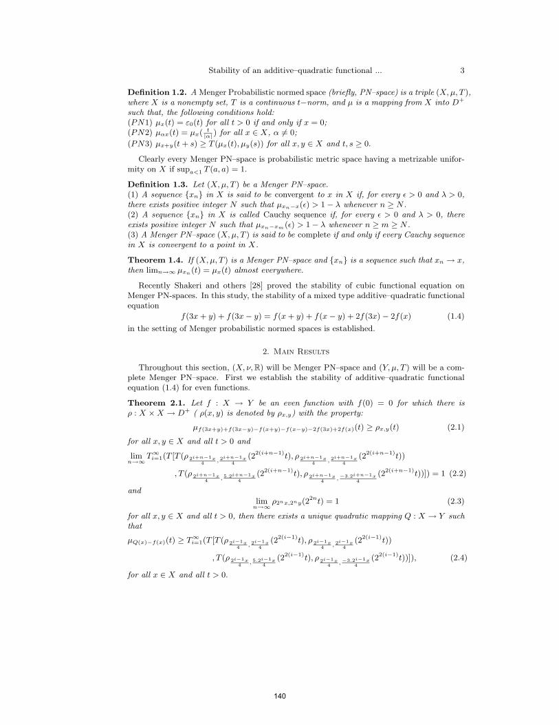
Stability of an additive–quadratic functional ... 3
Definition 1.2. A Menger Probabilistic normed space (briefly, PN–space) is a triple (X,µ, T ),where X is a nonempty set, T is a continuous t−norm, and µ is a mapping from X into D+
such that, the following conditions hold:(PN1) µx(t) = ε0(t) for all t > 0 if and only if x = 0;(PN2) µαx(t) = µx( t
|α| ) for all x ∈ X, α 6= 0;
(PN3) µx+y(t+ s) ≥ T (µx(t), µy(s)) for all x, y ∈ X and t, s ≥ 0.
Clearly every Menger PN–space is probabilistic metric space having a metrizable unifor-mity on X if supa<1 T (a, a) = 1.
Definition 1.3. Let (X,µ, T ) be a Menger PN–space.(1) A sequence xn in X is said to be convergent to x in X if, for every ε > 0 and λ > 0,there exists positive integer N such that µxn−x(ε) > 1− λ whenever n ≥ N .(2) A sequence xn in X is called Cauchy sequence if, for every ε > 0 and λ > 0, thereexists positive integer N such that µxn−xm(ε) > 1− λ whenever n ≥ m ≥ N .(3) A Menger PN–space (X,µ, T ) is said to be complete if and only if every Cauchy sequencein X is convergent to a point in X.
Theorem 1.4. If (X,µ, T ) is a Menger PN–space and xn is a sequence such that xn → x,then limn→∞ µxn(t) = µx(t) almost everywhere.
Recently Shakeri and others [28] proved the stability of cubic functional equation onMenger PN-spaces. In this study, the stability of a mixed type additive–quadratic functionalequation
f(3x+ y) + f(3x− y) = f(x+ y) + f(x− y) + 2f(3x)− 2f(x) (1.4)
in the setting of Menger probabilistic normed spaces is established.
2. Main Results
Throughout this section, (X, ν,R) will be Menger PN–space and (Y, µ, T ) will be a com-plete Menger PN–space. First we establish the stability of additive–quadratic functionalequation (1.4) for even functions.
Theorem 2.1. Let f : X → Y be an even function with f(0) = 0 for which there isρ : X ×X → D+ ( ρ(x, y) is denoted by ρx,y) with the property:
µf(3x+y)+f(3x−y)−f(x+y)−f(x−y)−2f(3x)+2f(x)(t) ≥ ρx,y(t) (2.1)
for all x, y ∈ X and all t > 0 and
limn→∞
T∞i=1(T [T (ρ 2i+n−1x4 , 2i+n−1x
4(22(i+n−1)t), ρ 2i+n−1x
4 , 2i+n−1x4
(22(i+n−1)t))
, T (ρ 2i+n−1x4 , 5.2i+n−1x
4(22(i+n−1)t), ρ 2i+n−1x
4 ,−3.2i+n−1x4
(22(i+n−1)t))]) = 1 (2.2)
and
limn→∞
ρ2nx,2ny(22nt) = 1 (2.3)
for all x, y ∈ X and all t > 0, then there exists a unique quadratic mapping Q : X → Y suchthat
µQ(x)−f(x)(t) ≥ T∞i=1(T [T (ρ 2i−1x4 , 2i−1x
4(22(i−1)t), ρ 2i−1x
4 , 2i−1x4
(22(i−1)t))
, T (ρ 2i−1x4 , 5.2i−1x
4(22(i−1)t), ρ 2i−1x
4 ,−3.2i−1x4
(22(i−1)t))]), (2.4)
for all x ∈ X and all t > 0.
140

4 M. Eshaghi Gordji, M. B. Savadkouhi and S. M. Vaezpour
Proof. By replacing y by x+ y in (2.1), we get
µf(4x+y)+f(2x−y)−f(2x+y)−f(y)−2f(3x)+2f(x)(t) ≥ ρx,x+y(t) (2.5)
for all x, y ∈ X. If we Replace y by −y in (2.5), we get
µf(4x−y)+f(2x+y)−f(2x−y)−f(y)−2f(3x)+2f(x)(t) ≥ ρx,x−y(t) (2.6)
for all x, y ∈ X. If we add (2.5) to (2.6), we have
µf(4x+y)+f(4x−y)−2f(y)−4f(3x)+4f(x)(t) ≥ T (ρx,x+y(t
2), ρx,x−y(
t
2)). (2.7)
Letting y = 0 in (2.7), we get the inequality
µ2f(4x)−4f(3x)+4f(x)(t) ≥ T (ρx,x(t
2), ρx,x(
t
2)) (2.8)
for all x ∈ X. Once again By letting y = 4x in (2.7), we obtain the inequality
µf(8x)−2f(4x)−4f(3x)+4f(x)(t) ≥ T (ρx,5x(t
2), ρx,−3x(
t
2)) (2.9)
for all x ∈ X. It follows from (2.8) and (2.9) that
µf(8x)−4f(4x)(t) ≥ T (T (ρx,x(t
4), ρx,x(
t
4)), T (ρx,5x(
t
4), ρx,−3x(
t
4))) (2.10)
for all x ∈ X. If we replace x by x4
in (2.10), we get
µf(2x)−4f(x)(t) ≥ T (T (ρ x4 , x
4(t
4), ρ x
4 , x4(t
4)), T (ρ x
4 , 5x4
(t
4), ρ x
4 ,−3x4
(t
4))) (2.11)
for all x ∈ X. Let
ψx,x(t) = T (T (ρ x4 , x
4(t
4), ρ x
4 , x4(t
4)), T (ρ x
4 , 5x4
(t
4), ρ x
4 ,−3x4
(t
4))) (2.12)
for all x ∈ X, then we obtain
µf(2x)−4f(x)(t) ≥ ψx,x(t) (2.13)
for all x ∈ X and all t > 0. Thus we have
µ f(2x)22
−f(x)(t) ≥ ψx,x(22t) (2.14)
for all x ∈ X and all t > 0. Hence,
µ f(2k+1x)
22(k+1) −f(2kx)
22k
(t) ≥ ψ2kx,2kx(22(k+1)t) (2.15)
for all x ∈ X and all k ∈ N. It follows that
µ f(2nx)22n −f(x)
(t) ≥ Tn−1k=0 (µ f(2k+1x)
22(k+1) −f(2kx)
22k
(t)) ≥ Tn−1k=0 (ψ2kx,2kx(22(k+1)t))
= Tni=1(ψ2i−1x,2i−1x(22it)) (2.16)
for all x ∈ X and t > 0. In order to prove the convergence of the sequence f(2nx)
22n , wereplace x with 2mx in (2.16) to find that
µ f(2n+mx)
22(n+m) −f(2mx)
22m
(t) ≥ Tni=1(ψ2i+m−1x,2i+m−1x(22(i+m)t)). (2.17)
Since the right hand side of the inequality tends to 1 as m and n tend to infinity, the
sequence f(2nx)
22n is a Cauchy sequence. Therefore, we may define Q(x) = limn→∞f(2nx)
22n
141
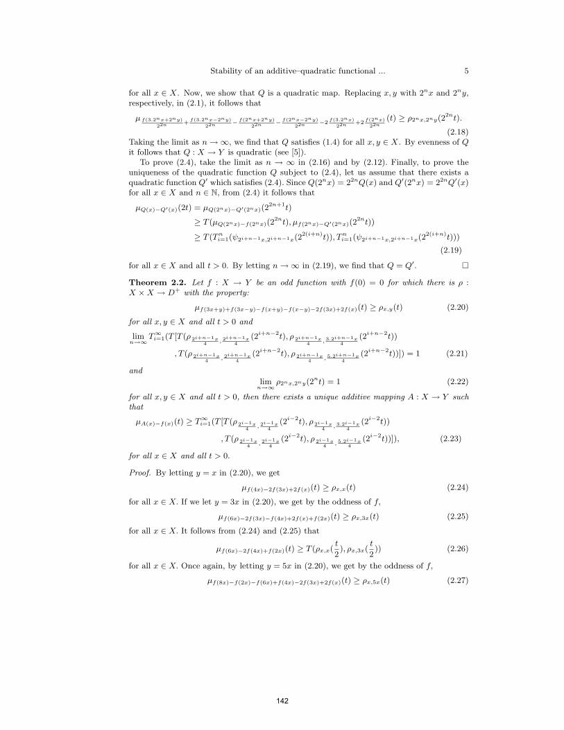
Stability of an additive–quadratic functional ... 5
for all x ∈ X. Now, we show that Q is a quadratic map. Replacing x, y with 2nx and 2ny,respectively, in (2.1), it follows that
µ f(3.2nx+2ny)22n +
f(3.2nx−2ny)22n − f(2nx+2ny)
22n − f(2nx−2ny)22n −2
f(3.2nx)22n +2
f(2nx)22n
(t) ≥ ρ2nx,2ny(22nt).
(2.18)Taking the limit as n→∞, we find that Q satisfies (1.4) for all x, y ∈ X. By evenness of Qit follows that Q : X → Y is quadratic (see [5]).
To prove (2.4), take the limit as n → ∞ in (2.16) and by (2.12). Finally, to prove theuniqueness of the quadratic function Q subject to (2.4), let us assume that there exists aquadratic function Q′ which satisfies (2.4). Since Q(2nx) = 22nQ(x) and Q′(2nx) = 22nQ′(x)for all x ∈ X and n ∈ N, from (2.4) it follows that
µQ(x)−Q′(x)(2t) = µQ(2nx)−Q′(2nx)(22n+1t)
≥ T (µQ(2nx)−f(2nx)(22nt), µf(2nx)−Q′(2nx)(2
2nt))
≥ T (Tni=1(ψ2i+n−1x,2i+n−1x(22(i+n)t)), Tn
i=1(ψ2i+n−1x,2i+n−1x(22(i+n)t)))
(2.19)
for all x ∈ X and all t > 0. By letting n→∞ in (2.19), we find that Q = Q′.
Theorem 2.2. Let f : X → Y be an odd function with f(0) = 0 for which there is ρ :X ×X → D+ with the property:
µf(3x+y)+f(3x−y)−f(x+y)−f(x−y)−2f(3x)+2f(x)(t) ≥ ρx,y(t) (2.20)
for all x, y ∈ X and all t > 0 and
limn→∞
T∞i=1(T [T (ρ 2i+n−1x4 , 2i+n−1x
4(2i+n−2t), ρ 2i+n−1x
4 , 3.2i+n−1x4
(2i+n−2t))
, T (ρ 2i+n−1x4 , 2i+n−1x
4(2i+n−2t), ρ 2i+n−1x
4 , 5.2i+n−1x4
(2i+n−2t))]) = 1 (2.21)
and
limn→∞
ρ2nx,2ny(2nt) = 1 (2.22)
for all x, y ∈ X and all t > 0, then there exists a unique additive mapping A : X → Y suchthat
µA(x)−f(x)(t) ≥ T∞i=1(T [T (ρ 2i−1x4 , 2i−1x
4(2i−2t), ρ 2i−1x
4 , 3.2i−1x4
(2i−2t))
, T (ρ 2i−1x4 , 2i−1x
4(2i−2t), ρ 2i−1x
4 , 5.2i−1x4
(2i−2t))]), (2.23)
for all x ∈ X and all t > 0.
Proof. By letting y = x in (2.20), we get
µf(4x)−2f(3x)+2f(x)(t) ≥ ρx,x(t) (2.24)
for all x ∈ X. If we let y = 3x in (2.20), we get by the oddness of f,
µf(6x)−2f(3x)−f(4x)+2f(x)+f(2x)(t) ≥ ρx,3x(t) (2.25)
for all x ∈ X. It follows from (2.24) and (2.25) that
µf(6x)−2f(4x)+f(2x)(t) ≥ T (ρx,x(t
2), ρx,3x(
t
2)) (2.26)
for all x ∈ X. Once again, by letting y = 5x in (2.20), we get by the oddness of f,
µf(8x)−f(2x)−f(6x)+f(4x)−2f(3x)+2f(x)(t) ≥ ρx,5x(t) (2.27)
142

6 M. Eshaghi Gordji, M. B. Savadkouhi and S. M. Vaezpour
for all x ∈ X. By (2.24) and using (2.26) and (2.27), we obtain
µf(8x)−2f(4x)(t) ≥ T [T (ρx,x(t
4), ρx,3x(
t
4)), T (ρx,x(
t
4), ρx,5x(
t
4))] (2.28)
for all x ∈ X. If we replace x by x4
in (2.28), we get that
µf(2x)−2f(x)(t) ≥ T [T (ρ x4 , x
4(t
4), ρ x
4 , 3x4
(t
4)), T (ρ x
4 , x4(t
4), ρ x
4 , 5x4
(t
4))] (2.29)
for all x ∈ X. Let
φx,x(t) = T [T (ρ x4 , x
4(t
4), ρ x
4 , 3x4
(t
4)), T (ρ x
4 , x4(t
4), ρ x
4 , 5x4
(t
4))] (2.30)
for all x ∈ X and all t > 0. Hence,
µf(2x)−2f(x)(t) ≥ φx,x(t) (2.31)
for all x ∈ X and t > 0. Thus, we have
µ f(2x)2 −f(x)
(t) ≥ φx,x(2t) (2.32)
for all x ∈ X. This implies that
µ f(2k+1x)2k+1 − f(2kx)
2k
(t) ≥ φ2kx,2kx(2k+1t) (2.33)
for all x ∈ X and all k ∈ N. Thus we have
µ f(2nx)2n −f(x)
(t) ≥ Tn−1k=0 (µ f(2k+1x)
2k+1 − f(2kx)2k
(t)) ≥ Tn−1k=0 (φ2kx,2kx(2k+1t))
= Tni=1(φ2i−1x,2i−1x(2it)) (2.34)
for all x ∈ X and t > 0. In order to prove the convergence of the sequence f(2nx)2n , we
replace x with 2mx in (2.34) to find that
µ f(2n+mx)2n+m − f(2mx)
2m(t) ≥ Tn
i=1(φ2i+m−1x,2i+m−1x(2i+mt)). (2.35)
Since the right hand side of the inequality tends to 1 as m and n tend to infinity, the
sequence f(2nx)2n is a Cauchy sequence. Therefore, we may define A(x) = limn→∞
f(2nx)2n
for all x ∈ X. Now, we show that A is a additive map. Replacing x, y with 2nx and 2nyrespectively in (2.20), it follows that
µ f(3.2nx+2ny)2n +
f(3.2nx−2ny)2n − f(2nx+2ny)
2n − f(2nx−2ny)2n −2
f(3.2nx)2n +2
f(2nx)2n
(t) ≥ ρ2nx,2ny(2nt).
(2.36)Taking the limit as n → ∞, we find that A satisfies (1.4) for all x, y ∈ X. Therefore themapping A : X → Y is additive (see [5]). To prove (2.23), take the limit as n → ∞ in(2.34) and by (2.30). Finally, to prove the uniqueness of the additive function A subject to(2.23), let us assume that there exists a additive function A′ which satisfies (2.23). SinceA(2nx) = 2nA(x) and A′(2nx) = 2nA′(x) for all x ∈ X and n ∈ N, from (2.23) it followsthat
µA(x)−A′(x)(2t) = µA(2nx)−A′(2nx)(2n+1t)
≥ T (µA(2nx)−f(2nx)(2nt), µf(2nx)−A′(2nx)(2
nt))
≥ T (Tni=1(φ2i+n−1x,2i+n−1x(2i+nt)), Tn
i=1(φ2i+n−1x,2i+n−1x(2i+nt))) (2.37)
for all x ∈ X and all t > 0. By letting n→∞ in (2.37), we find that A = A′.
143
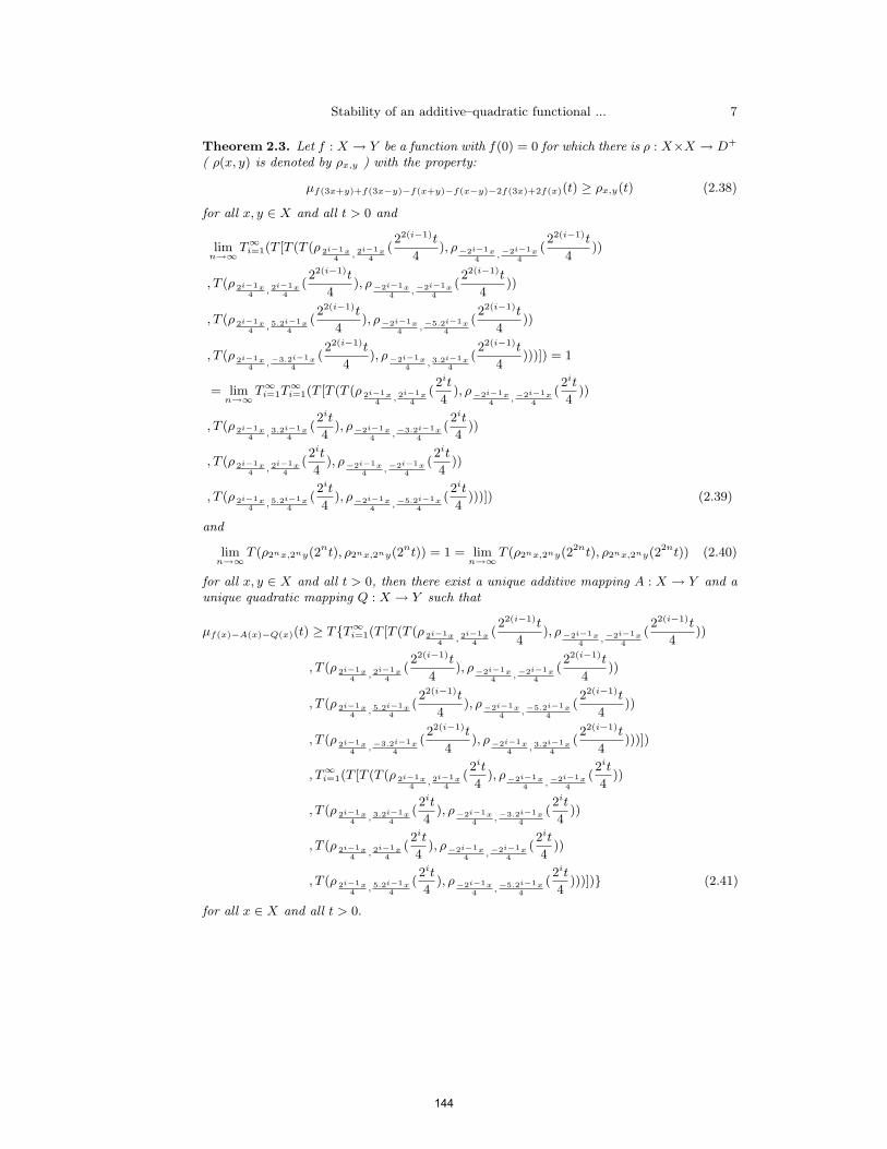
Stability of an additive–quadratic functional ... 7
Theorem 2.3. Let f : X → Y be a function with f(0) = 0 for which there is ρ : X×X → D+
( ρ(x, y) is denoted by ρx,y ) with the property:
µf(3x+y)+f(3x−y)−f(x+y)−f(x−y)−2f(3x)+2f(x)(t) ≥ ρx,y(t) (2.38)
for all x, y ∈ X and all t > 0 and
limn→∞
T∞i=1(T [T (T (ρ 2i−1x4 , 2i−1x
4(22(i−1)t
4), ρ−2i−1x
4 ,−2i−1x4
(22(i−1)t
4))
, T (ρ 2i−1x4 , 2i−1x
4(22(i−1)t
4), ρ−2i−1x
4 ,−2i−1x4
(22(i−1)t
4))
, T (ρ 2i−1x4 , 5.2i−1x
4(22(i−1)t
4), ρ−2i−1x
4 ,−5.2i−1x4
(22(i−1)t
4))
, T (ρ 2i−1x4 ,−3.2i−1x
4(22(i−1)t
4), ρ−2i−1x
4 , 3.2i−1x4
(22(i−1)t
4)))]) = 1
= limn→∞
T∞i=1T∞i=1(T [T (T (ρ 2i−1x
4 , 2i−1x4
(2it
4), ρ−2i−1x
4 ,−2i−1x4
(2it
4))
, T (ρ 2i−1x4 , 3.2i−1x
4(2it
4), ρ−2i−1x
4 ,−3.2i−1x4
(2it
4))
, T (ρ 2i−1x4 , 2i−1x
4(2it
4), ρ−2i−1x
4 ,−2i−1x4
(2it
4))
, T (ρ 2i−1x4 , 5.2i−1x
4(2it
4), ρ−2i−1x
4 ,−5.2i−1x4
(2it
4)))]) (2.39)
and
limn→∞
T (ρ2nx,2ny(2nt), ρ2nx,2ny(2nt)) = 1 = limn→∞
T (ρ2nx,2ny(22nt), ρ2nx,2ny(22nt)) (2.40)
for all x, y ∈ X and all t > 0, then there exist a unique additive mapping A : X → Y and aunique quadratic mapping Q : X → Y such that
µf(x)−A(x)−Q(x)(t) ≥ TT∞i=1(T [T (T (ρ 2i−1x4 , 2i−1x
4(22(i−1)t
4), ρ−2i−1x
4 ,−2i−1x4
(22(i−1)t
4))
, T (ρ 2i−1x4 , 2i−1x
4(22(i−1)t
4), ρ−2i−1x
4 ,−2i−1x4
(22(i−1)t
4))
, T (ρ 2i−1x4 , 5.2i−1x
4(22(i−1)t
4), ρ−2i−1x
4 ,−5.2i−1x4
(22(i−1)t
4))
, T (ρ 2i−1x4 ,−3.2i−1x
4(22(i−1)t
4), ρ−2i−1x
4 , 3.2i−1x4
(22(i−1)t
4)))])
, T∞i=1(T [T (T (ρ 2i−1x4 , 2i−1x
4(2it
4), ρ−2i−1x
4 ,−2i−1x4
(2it
4))
, T (ρ 2i−1x4 , 3.2i−1x
4(2it
4), ρ−2i−1x
4 ,−3.2i−1x4
(2it
4))
, T (ρ 2i−1x4 , 2i−1x
4(2it
4), ρ−2i−1x
4 ,−2i−1x4
(2it
4))
, T (ρ 2i−1x4 , 5.2i−1x
4(2it
4), ρ−2i−1x
4 ,−5.2i−1x4
(2it
4)))]) (2.41)
for all x ∈ X and all t > 0.
144

8 M. Eshaghi Gordji, M. B. Savadkouhi and S. M. Vaezpour
Proof. Let
fe(x) =1
2[f(x) + f(−x)]
for all x ∈ X. Then fe(0) = 0, fe(−x) = fe(x), and
µfe(3x+y)+fe(3x−y)−fe(x+y)−fe(x−y)−2fe(3x)+2fe(x)(t) ≥ T (ρx,y(t), ρ−x,−y(t)) (2.42)
for all x, y ∈ X. Hence, in view of Theorem 2.1, there exists a unique quadratic functionQ : X → Y such that
µfe(x)−Q(x)(t) ≥ T∞i=1(T [T (T (ρ 2i−1x4 , 2i−1x
4(22(i−1)t
4), ρ−2i−1x
4 ,−2i−1x4
(22(i−1)t
4))
, T (ρ 2i−1x4 , 2i−1x
4(22(i−1)t
4), ρ−2i−1x
4 ,−2i−1x4
(22(i−1)t
4))
, T (ρ 2i−1x4 , 5.2i−1x
4(22(i−1)t
4), ρ−2i−1x
4 ,−5.2i−1x4
(22(i−1)t
4))
, T (ρ 2i−1x4 ,−3.2i−1x
4(22(i−1)t
4), ρ−2i−1x
4 , 3.2i−1x4
(22(i−1)t
4)))]).
(2.43)
Let
fo(x) =1
2[f(x)− f(−x)]
for all x ∈ X. Then fo(0) = 0, fo(−x) = −fo(x), and
µfo(3x+y)+fo(3x−y)−fo(x+y)−fo(x−y)−2fo(3x)+2fo(x)(t) ≥ T (ρx,y(t), ρ−x,−y(t)) (2.44)
for all x, y ∈ X. From Theorem 2.2, it follows that there exist a unique additive mappingA : X → Y such that
µfo(x)−A(x)(t) ≥ T∞i=1(T [T (T (ρ 2i−1x4 , 2i−1x
4(2it
4), ρ−2i−1x
4 ,−2i−1x4
(2it
4))
, T (ρ 2i−1x4 , 3.2i−1x
4(2it
4), ρ−2i−1x
4 ,−3.2i−1x4
(2it
4))
, T (ρ 2i−1x4 , 2i−1x
4(2it
4), ρ−2i−1x
4 ,−2i−1x4
(2it
4))
, T (ρ 2i−1x4 , 5.2i−1x
4(2it
4), ρ−2i−1x
4 ,−5.2i−1x4
(2it
4)))]).
(2.45)
Now it is obvious that (2.41) holds true for all x ∈ A, and the proof of theorem is complete.
References
[1] J. Aczel and J. Dhombres, Functional equations in several variables, Cambridge Univ.Press, 1989.
[2] P. W. Cholewa, Remarks on the stability of functional equations, Aequationes Math. 27(1984), 76–86.
[3] S. S. Chang, Y. J. Cho and S. M. Kang, Nonlinear operator theory in probabilisticmetric spaces, Nova Science Publishers, Inc. New York, 2001.
[4] S. Czerwik, On the stability of the quadratic mapping in normed spaces, Abh. Math.Sem. Univ. Hamburg 62 (1992), 59–64.
145
Stability of an additive–quadratic functional ... 9
[5] M. Eshaghi Gordji and M. Bavand Savadkouhi, Stability of a mixed type additive andquadratic functional equation in random normed spaces, submitted.
[6] M. Eshaghi Gordji and M. Bavand Savadkouhi, Stability of mixed type cubic and quarticfunctional equations in random normed spaces, Journal of Inequalities and Applications,Volume 2009, Article ID 527462, 9 pages, doi:10.1155/2009/527462.
[7] M. Eshaghi Gordji, A. Ebadian and S. Zolfaghari, Stability of a functional equationderiving from cubic and quartic functions, Abstract and Applied Analysis Volume 2008,Article ID 801904, 17 pages.
[8] M. Eshaghi Gordji and H. Khodaei, Solution and stability of generalized mixed typecubic, quadratic and additive functional equation in quasi–Banach spaces, NonlinearAnalysis, 71 (2009) 5629–5643.
[9] Z. Gajda, On stability of additive mappings, Internat. J. Math. Math. Sci. 14 (1991),431–434.
[10] P. Gavruta, A generalization of the Hyers-Ulam-Rassias stability of approximately ad-ditive mappings, J. Math. Anal. Appl. 184 (1994), 431–436.
[11] A. Gilanyi, On Hyers–Ulam stability of monomial functional equations. Abh. Math.Sem. Univ. Hamburg, 68 (1998), 321–328.
[12] A. Gilanyi, Hyers–Ulam stability of monomial functional equations on a general domain.Proc. Natl. Acad. Sci. USA, 96 (1999), no. 19, 10588–10590 (electronic).
[13] A. Grabiec, The generalized Hyers-Ulam stability of a class of functional equations,Publ. Math. Debrecen 48 (1996), 217–235.
[14] O. Hadzic, E. Pap and M. Budincevic, Countable extension of triangular norms andtheir applications to the fixed point theory in probabilistic metric spaces, Kybernetica,38 (3) (2002), 363–381.
[15] D. H. Hyers, G. Isac and Th. M. Rassias, Stability of functional equations in severalvariables, Birkhaer, Basel, 1998.
[16] D. H. Hyers, On the stability of the linear functional equation, Proc. Natl. Acad. Sci.27 (1941), 222–224.
[17] G. Isac and Th. M. Rassias, On the Hyers-Ulam stability of ψ-additive mappings, J.Approx. Theory 72 (1993), 131–137.
[18] Pl. Kannappan, Quadratic functional equation and inner product spaces, Results Math.27 (1995), 368–372.
[19] D. Mihet and V. Radu, On the stability of the additive Cauchy functional equation inrandom normed spaces, J. Math. Anal. Appl. 343 (2008), 567-572.
[20] D. Mihet, The probabilistic stability for a functional equation in a single variable, ActaMath. Hungar. 2008 DOI: 10.1007/s10474-008-8101-y.
[21] D. Mihet, The fixed point method for fuzzy stability of the Jensen functional equation,Fuzzy Sets and Systems, doi:10.1016/j.fss.2008.06.014.
[22] A. K. Mirmostafee and M. S. Moslehian, Fuzzy versions of Hyers-Ulam-Rassias theorem,Fuzzy Sets and Systems, 159 (2008), 720–729.
[23] A. K. Mirmostafaee, M. S. Moslehian, Fuzzy approximately cubic mappings, Inform.Sci. (2008), doi:10.1016/j.ins.2008.05.032.
[24] Th. M. Rassias, On the stability of functional equations and a problem of Ulam, ActaMath. Appl. 62 (2000), 23–130.
[25] Th. M. Rassias, On the stability of functional equations in Banach spaces, J. Math.Anal. Appl. 251 (2000), 264–284.
[26] Th. M. Rassias, On the stability of the linear mapping in Banach spaces, Proc. Amer.Math. Soc. 72 (1978), 297–300.
146

10 M. Eshaghi Gordji, M. B. Savadkouhi and S. M. Vaezpour
[27] B. Schweizer and A. Sklar, Probabilistic Metric Spaces, Elsevier, North Holand, NewYork, 1983.
[28] S. Shakeri, R. Saadati, Gh. Sadeghi and S. M. Vaezpour, Stability of the cubic functionalequation in menger probabilistic normed space, Journal of Applied sciences. 9 (2009),1759–1797.
[29] F. Skof, Propriet locali e approssimazione di operatori, Rend. Sem. Mat. Fis. Milano,53 (1983), 113-129.
[30] S. M. Ulam, Problems in modern mathematics, Chapter VI, science ed., Wiley, NewYork, 1940.
147

ON NEW CLASSES OF DOUBLE SEQUENCE SPACES DEFINEDBY ORLICZ FUNCTION
AYHAN ESI
Abstract. In this paper we introduce new double sequence spaces via Orliczfunction and examine some properties of the resulting these spaces.
1. INTRODUCTION
Before we enter the motivation for this paper and the presentation of themain results we give some preliminaries.
Recall in [11] that an Orlicz functionM is continuous, convex, nondecreasingfunction dene for x > 0 such that M(0) = 0 and M(x) > 0. If convexity of Orliczfunction is replaced by M(x + y) M (x) + M (y) then this function is calledthe modulus function and characterized by Ruckle [16] :An Orlicz function M issaid to satisfy 2 condition for all values u, if there exists K > 0 such thatM(2u) KM(u); u 0:
Remark. An Orlicz function satises the inequality M (x) M (x) forall with 0 < < 1:
Lindenstrauss and Tzafriri [10] used the idea of Orlicz function to constructthe sequence space
lM =
((xi) :
1Xi=1
M
jxijr
<1; for some r > 0
);
which is a Banach space normed by
k(xi)k = inf(r > 0 :
1Xi=1
M
jxijr
1
):
The space lM is closely related to the space lp, which is an Orlicz sequence spacewith M (x) = jxjp ; for 1 p <1:
In the later stage di¤erent Orlicz sequence spaces were introduced and stud-ied by Tripathy and Mahanta [5] ; Esi [1 2] ; Esi and Et [3] ; Parashar and Choud-hary [12] and many others.
By the convergence of a double sequence we mean the convergence on thePringsheim sense that is, a double sequence x = (xij) has Pringsheim limit L(denoted by P limx = L) provided that given " > 0 there exists n 2 N such thatjxij Lj < " whenever i; j > n; [4] :We shall write more briey as "Pconvergent".
The initial works on double sequences is found in Bromwich [14] : Later onit was studied by Hardy [8] ; Moricz [6] ; Moricz and Rhoades [7] and many others.
Date : April 26, 2011.2000 Mathematics Subject Classication. 40A05, 40B05, 46E30.Key words and phrases. P-convergent, double sequence space,Orlicz function.
1
148
JOURNAL OF APPLIED FUNCTIONAL ANALYSIS, VOL.7, NO’S 1-2,148-156,COPYRIGHT 2012 EUDOXUS PRESS,LLC
2 AYHAN ESI
Hardy [8] introduced the notion of regular convergence for double sequences. Theconcept of paranormed sequences was studied by Nakano [9] and Simons [13] at theinitial stage. Later on it was studied by many others.
The double sequence x = (xij) is bounded if there exists a positive numberM such that jxij j < M for all i; j 2 N. Let l21 the space of all bounded double suchthat
kxijk(1;2) = supi;jjxij j <1:
Throughout the paper, w2 (X) denotes the spaces of all double sequences inX, where (X; q) denotes a seminormed space, seminormed by q. The zero doublesequence is denoted by in X.
2:DEFINITIONS AND BACKGROUND
Let Ps denotes the class of all subsets of N, those do not contain more than selements and fng represents a non-decreasing sequence of real numbers such thatnn+1 (n+ 1)n for all n 2 N:
The sequence space m () introduced by Sargent [15] is dened as follows:
m () =
(x = (xk) : kxkkm() = sup
s1;2Ps
1
s
Xi2
jxij <1)
and studied some of its properties and obtained its relationship with the space lp:A double sequence space E is said to be solid or normal if (ijxij) 2 E;
whenever (xij) 2 E for all double sequences (ij) of scalars such that jij j 1 forall i; j 2 N:
A double sequence space E is said to be symmetric if (xij) 2 E impliesx(i)(j)
2 E; where is a permutation of the elements of N:
Let K = f(in; jk) : n; k 2 N; i1 < i2 < i3 < :::: and j1 < j2 < j3 < :::g N N and E be a double sequence space. A K step space of E is a sequencespace
EK = f(xinjk) : (xij) 2 Eg :
A canonical pre-image of a sequence (xinjk) 2 E is a sequence (yij) 2 Edened as follows:
yij = fxij ; if (i; j) 2 K0; otherwise
:
A canonical pre-image of a step space EK is a set of canonical pre-images ofall elements in EK :
A double sequence space E is said to be monotone if E contains the canonicalpre-images of all its step spaces.
Lemma. A double sequence space E is solid implies E is monotone.Let Pst denotes the class of all subsets of N N; those do not contain
more that s t elements. Throughout the paper fn;mg represent a non-decreasingdouble sequence of real numbers such that nn+1;m (n+ 1)n;m and mn;m+1 (m+ 1)n;m: In this paper we introduce the following double sequence spaces: LetM be an Orlicz function and a p = (pij) be a bounded double sequence of positive
149

ON NEW CLASSES OF DOUBLE SEQUENCE SPACES DEFINED BY ORLICZ FUNCTION 3
real numbers such that 0 < Ho = infi;j pij pij supi;j pij = H <1; then
l21 (M; q; p) =
x = (xij) 2 w2 (X) : sup
i;j
hMqxijr
ipij<1; for some r > 0
;
l2p (M; q) =
8<:x = (xij) 2 w2 (X) :1X
i;j=1;1
hMqxijr
ipij<1; for some r > 0
9=; ;
m2 (M;; q; p) =
8<:x = (xij) 2 w2 (X) : sups;t1;2Pst
1
s;t
X(i;j)2
hMqxijr
ipij<1; for some r > 0
9=; :
The following inequality will be used throughout the paper
jaij + bij jpij max1; 2H1
(jaij jpij + jbij jpij )
where aij and bij are complex numbers and H = supi;j pij <1:It is easy to see that the double sequence space l2p (M; q) is a seminormed
space, seminormed by
g ((xij)) = inf
8<:r pijJ > 0 :1X
i;j=1;1
Mqxijr
1
9=; ; where J = max1; 2H1
3:MAIN RESULTS
In this section we prove some results involving the double sequence spacesm2 (M;; q; p) ; l2p (M; q) and l21 (M; q; p) :
Theorem 3.1. m2 (M;; q; p) and l21 (M; q; p) are linear spaces.Proof. Let (xij) ; (yij) 2 m2 (M;; q; p) and ; 2 C: Then there exists
positive numbers r1 and r2 such that
sups;t1;2Pst
1
s;t
X(i;j)2
M
q
xijr1
pij<1
and
sups;t1;2Pst
1
s;t
X(i;j)2
M
q
yijr2
pij<1:
Let r3 = max (2 jj r1; 2 jj r2) : Since M is non-decreasing convex functionand q is a seminorm, we haveX
(i;j)2
M
q
xij + yij
r3
pij
X
(i;j)2
M
q
xijr3
+ q
yijr3
pij
max1; 2H1
X(i;j)2
M
q
xijr1
pij+max
1; 2H1
M
q
yijr2
pij:
150

4 AYHAN ESI
So,
sups;t1;2Pst
1
s;t
X(i;j)2
M
q
xij + yij
r3
pij
sups;t1;2Pst
1
s;t
X(i;j)2
M
q
xijr1
pij+ sups;t1;2Pst
1
s;t
X(i;j)2
M
q
yijr2
pij<1;
therefore (xij + yij) 2 m2 (M;; q; p) : Hence m2 (M;; q; p) is a linear space.The proof for the case l21 (M; q; p) is a routine work in view of the above
proof.Theorem 3.2. The space m2 (M;; q; p) is a seminormed space, semi-
normed by
h ((xij)) = inf
8<:r pijJ > 0 : sups;t1;2Pst
1
s;t
X(i;j)2
Mqxijr
1
9=; ; where J = max1; 2H1
:
Proof. Clearly h ((xij)) 0 for all (xij) 2 m2 (M;; q; p) and h () = 0:Let r1 > 0 and r2 > 0 be such that
sups;t1;2Pst
1
s;t
X(i;j)2
M
q
xijr1
1
and
sups;t1;2Pst
1
s;t
X(i;j)2
M
q
yijr2
1:
Let r = r1 + r2: Then we have
sups;t1;2Pst
1
s;t
X(i;j)2
M
q
xij + yij
r
= sups;t1;2Pst
1
s;t
X(i;j)2
M
q
xij + yijr1 + r2
sups;t1;2Pst
1
s;t
X(i;j)2
r1
r1 + r2M
q
xijr1
+
r2r1 + r2
M
q
yijr2
r1r1 + r2
sup
s;t1;2Pst
1
s;t
X(i;j)2
M
q
xijr1
+
r2
r1 + r2
sup
s;t1;2Pst
1
s;t
X(i;j)2
M
q
yijr2
1:
Since the r0s are nonnegative, so we have
h ((xij) + (yij)) = inf
8<:r pijJ > 0 : sups;t1;2Pst
1
s;t
X(i;j)2
M
q
xij + yij
r
1
9=;
151

ON NEW CLASSES OF DOUBLE SEQUENCE SPACES DEFINED BY ORLICZ FUNCTION 5
inf
8<:r pijJ1 > 0 : sups;t1;2Pst
1
s;t
X(i;j)2
M
q
xijr1
1
9=;+ inf
8<:r pijJ2 > 0 : sups;t1;2Pst
1
s;t
X(i;j)2
M
q
xijr2
1
9=;= h ((xij)) + h ((yij)) :
Next for 2 C; without loss of generality, let 6= 0; then
h ((xij)) = inf
8<:r pijJ > 0 : sups;t1;2Pst
1
s;t
X(i;j)2
M
q
xijr
1
9=;= inf
8<:(jj ) pijJ > 0 : sups;t1;2Pst
1
s;t
X(i;j)2
M
q
xij
1
9=; ;where =r
jj
Hence we geth ((xij)) max (1; jj)h ((xij)) :
This completes the proof of the theorem.The proof of the following result is a consequence of the above theorem.Proposition 3.3. The double sequence space l21 (M; q; p) is a seminormed
space, seminormed by
f ((xij)) = inf
rpijJ > 0 : sup
i;jMqxijr
1
; where J = max
1; 2H1
Theorem 3.4. m2 (M;; q; p) m2 (M; ; q; p) if and only if sups;t
s;t s;t
<1:
Proof. Let sups;ts;t s;t
<1 and (xij) 2 m2 (M;; q; p) : Then
sups;t1;2Pst
1
s;t
X(i;j)2
hMqxijr
ipij<1; for some r > 0:
So,
sups;t1;2Pst
1
s;t
X(i;j)2
hMqxijr
ipijsups;t
s;t s;t
sup
s;t1;2Pst
1
s;t
X(i;j)2
hMqxijr
ipij<1:
Therefore (xij) 2 m2 (M; ; q; p) : Hence m2 (M;; q; p) m2 (M; ; q; p) :
Conversely, let m2 (M;; q; p) m2 (M; ; q; p) : Suppose that sups;ts;t s;t
=
1. Then there exists a sequence of natural numbers (sij) such that Plimi;jsi;tj si;tj
=
1: Let (xij) 2 m2 (M;; q; p) : Then there exists r > 0 such that
sups;t1;2Pst
1
s;t
X(i;j)2
hMqxijr
ipij<1:
Now, we have
sups;t1;2Pst
1
s;t
X(i;j)2
hMqxijr
ipijsupi;j
si;tj si;tj
sup
i;j1;2Psitj
1
si;tj
X(i;j)2
hMqxijr
ipij=1:
Therefore (xij) =2 m2 (M; ; q; p) : This is a contradiction. Hence sups;ts;t s;t
<1 .
152
6 AYHAN ESI
The following result is a consequence of Theorem 3.4.Corollary 3.5. Let M be an Orlicz function. Then m2 (M;; q; p) =
m2 (M; ; q; p) if and only if sups;ts;t s;t
<1 and sups;t s;ts;t
<1 for all s; t = 1; 2; ::::Theorem 3.6. LetM;M1;M2 be Orlicz functions satisfying2condition:
Then(i) m2 (M1; ; q; p) m2 (MoM1; ; q; p) ;(ii) m2 (M1; ; q; p) \m2 (M2; ; q; p) m2 (M1 +M2; ; q; p) :Proof. (i) Let (xij) 2 m2 (M1; ; q; p) : Then there exists r > 0 such that
sups;t1;2Pst
1
s;t
X(i;j)2
hM1
qxijr
ipij<1:
Let 0 < " < 1 and with 0 < < 1 such that M (t) < " for 0 t < : Letyij =M1
qxijr
and for any 2 Pst; letX
(i;j)2
[M (yij)]pij =
X1
[M (yij)]pij +
X2
[M (yij)]pij
where the rst summation is over yij and the second is over yij > : By theremark we have(3.1)X
1
M (yij) max1; [M (1)]
HX
1
(yij)pij max
1; [M (2)]
HX
1
(yij)pij
For yij >
yij < yij1 1 + yij1;
since M is non-decreasing and convex, so
M (yij) < M1 + yij
1 < 1
2M (2) +
1
2M2yij
1 :Since M satises 2 condition, so
M (yij) <K
2yij
1M (2) +K
2yij
1M (2) = Kyij1M (2) :
Hence,
(3.2)X2
[M (yij)]pij max
1;K1M (2)
HX2
(yij)pij :
By (3:1) and (3:2) we have (xij) 2 m2 (MoM1; ; q; p) : Thus m2 (M1; ; q; p) m2 (MoM1; ; q; p) :
(ii) Let (xij) 2 m2 (M1; ; q; p) \m2 (M2; ; q; p) : Then there exists r > 0such that
sups;t1;2Pst
1
s;t
X(i;j)2
hM1
qxijr
ipij<1
and
sups;t1;2Pst
1
s;t
X(i;j)2
hM2
qxijr
ipij<1:
The rest of the proof follows from the equalityX(i;j)2
h(M1 +M2)
qxijr
ipij
153

ON NEW CLASSES OF DOUBLE SEQUENCE SPACES DEFINED BY ORLICZ FUNCTION 7
max1; 2H1
X(i;j)2
hM1
qxijr
ipij+max
1; 2H1
X(i;j)2
hM2
qxijr
ipij:
This completes the proof.Taking M1 (x) = x in above theorem, we have the following result.Corollary 3.7. Let M be an Orlicz function satisfying 2 condition,
then m2 (; q; p) m2 (M;; q; p) :From Theorem 3.4. and Corollary 3.7., we have:Corollary 3.8. Let M be an Orlicz function satisfying 2 condition,
then m2 (; q; p) m2 (M; ; q; p) if and only if sups;ts;t s;t
<1:Theorem 3.9. The double space m2 (M;; q; p) is solid and symmetric.Proof. Let (xij) 2 m2 (M;; q; p) : Then
(3.3) sups;t1;2Pst
1
s;t
X(i;j)2
hMqxijr
ipij<1:
Let (ij) be a double sequence of scalars with jij j 1 for all i; j 2 N: Then theresult follows from (3.3) and the following inequalityX(i;j)2
M
q
ijxijr
pij
X(i;j)2
hjij jM
qxijr
ipij(by the Remark)
X
(i;j)2
hMqxijr
ipij:
The symmetricity of the space follows from the denition of the double spacem2 (M;; q; p) and symmetric double sequence space.
The following result follows from Theorem 3.9 and the Lemma.Corollary 3.10. The double space m2 (M;; q; p) is monotone.The proof of the following result is a routine work.Proposition 3.11. The double spaces l2p (M; q) and l21 (M; q; p) are solid
and as such are monotone.Theorem 3.12. l2p (M; q) m2 (M;; q; p) l21 (M; q; p) :
Proof. Let (xij) 2 l2p (M; q) : Then we have
(3.4)1X
i;j=1;1
hMqxijr
ipij<1; for some r > 0:
Since fn;mg is monotonic increasing, so we have1
s;t
X(i;j)2
hMqxijr
ipij 1
1;1
X(i;j)2
hMqxijr
ipij<1:
Hence
sups;t1;2Pst
1
s;t
X(i;j)2
hMqxijr
ipij<1:
Thus (xij) 2 m2 (M;; q; p) . Therefore l2p (M; q) m2 (M;; q; p) : Next let (xij) 2m2 (M;; q; p) : Then we have
sups;t1;2Pst
1
s;t
X(i;j)2
hMqxijr
ipij<1; for some r > 0.
154
8 AYHAN ESI
So,
supi;j2N
1
1;1
hMqxijr
ipij<1; for some r > 0 ( on taking cardinality of to be 1) :
Therefore (xij) 2 l21 (M; q; p) : Hencem2 (M;; q; p) l21 (M; q; p) : This completesthe proof.
Theorem 3.13.(i) m2 (M;; q; p) = l2p (M; q) if and only if sups;t1 s;t <1:
(ii) m2 (M;; q; p) = l21 (M; q; p) if and only if sups;t1sts;t
<1:Proof.(i) It is clear that m2 (M; ; q; p) = l2p (M; q) when s;t = 1 for
all s; t 2 N: By Theorem 3.4., m2 (M;; q; p) m2 (M; ; q; p) if and only ifsups;t
s;t s;t
< 1 i.e. sups;t s;t < 1: By Theorem 3.11., m2 (M;; q; p) = l2p (M; q)
if and only if sups;t s;t <1:(ii) We have m2 (M; ; q; p) = l21 (M; q) if s;t = st for all s; t 2 N: By
Theorem 3.4. and Theorem 3.11., it follows that m2 (M;; q; p) = l21 (M; q; p) ifand only if sups;t1
sts;t
<1:This completes the proof.The proof of the following result is routine work.Proposition 3.14. Let M be an Orlicz function, q1 and q2 be seminorms.
Then(i) m2 (M;; q1; p) \m2 (M;; q2; p) m2 (M;; q1 + q2; p) ;(ii) If q1 is stronger than q2; then m2 (M;; q1; p) m2 (M;; q2; p) ;(iii) l21 (M; q1; p) \ l21 (M; q2; p) l21 (M; q1 + q2; p) ;(iv) If q1 is stronger than q2; then l21 (M; q1; p) l21 (M; q2; p) ;(v) l2p (M; q1) \ l2p (M; q2) l2p (M; q1 + q2) ;
(vi) If q1 is stronger than q2; then l2p (M; q1) l2p (M; q2) :
4:PARTICULAR CASES
If one considers a normed linear space (X; k:k) instead of a seminormedspace (X; q) ; then one will get m2 (M;; k:k ; p) ; which will be a normed linearspace, normed by
k(xij)k = inf
8<:r pijJ > 0 : sups;t1;2Pst
1
s;t
X(i;j)2
M xij
r
19=; ;where J = max
1; 2H1
:
The double space m2 (M;; k:k ; p) will be a solid, monotone and symmetric space.Further most of the results proved in the previous section will be true for this spacetoo.
References
[1] A.Esi, Some new sequence spaces dened by Orlicz functions, Bull.Inst.Math.Acad.Sinica,27(1)(1999), 71-76.
[2] A.Esi, On a class of new type di¤erence sequences related to the space lp; Far EastJ.Math.Sci.(FJMS), 13(2)(2004), 167-172.
[3] A.Esi and M.Et, Some new sequence spaces dened b a sequence of Orlicz functions, IndianJ.Pure Appl.Math., 31(8)(2000), 967-972.
[4] A.Pringsheim, Zur Theori der zweifach unendlichen Zahlenfolgen, Math.Ann.53(1900), 289-321.
155
ON NEW CLASSES OF DOUBLE SEQUENCE SPACES DEFINED BY ORLICZ FUNCTION 9
[5] B.C.Tripathy and S.Mahanta, On a class of sequences related to the space dened by Orliczfunctions, Soochow J.Math., 29(4)(2003), 379-391.
[6] F.Moricz, Extension of the spaces c and co from single to double sequences, ActaMath.Hungarica, 57(1-2)(1991), 129-136.
[7] F.Moricz and B.E.Rhoades, Almost convergence of double sequences ant strong regularity ofsummability matrices,Math. Proc.Camb.Phil.Soc.,104(1988),283-294.
[8] G.H.Hardy, On the convergence of certain multiple series, Proc.Camb.Phil.Soc., 19(1917),86-95.
[9] H.Nakano, Modular sequence spaces, Proc.Japan Acad., 27(1951), 508-512.[10] J.Lindenstrauss and L.Tzafriri, On Orlicz sequence spaces, Israel J.Math., 10(1971), 379-390.[11] M.A.Krasnoselski and Y.B.Rutickii, Convex function and Orlicz spaces, Groningen, Neder-
land, 1961.[12] S.D.Parashar and B.Choudhary, Sequence spaces dened by Orlicz functions, Indian J.Pure
Appl.Math., 25(1994), 419-428.[13] S.Simons, The sequence spaces l (pv) and m (pv) ; Proc.London Math.Soc., 15(3)(1965), 422-
436.[14] T.J.IA.Bromwich, An Introduction to the Theory of Innite Series, MacMillan and Co.Ltd.
New York, 1965.[15] W.L.C.Sargent, Some sequence spaces related to spaces lp; J.London Math.Soc., 35(1960),
161-171.[16] W.H.Ruckle, FK-spaces in which the sequence of coordinate vectors is bounded,
Canad.J.Math.,25(1973), 973-978.
Adiyaman University, Science and Art Faculty, Department of Mathematics, 02040,Adiyaman, Turkey
E-mail address : [email protected]
156

On the convergence of variational
iteration method for the solution of
partial differential equations of
fractional order
M. Zandy∗ and A. Aminataei†
Department of Mathematics, K. N. Toosi University of Technology,
P.O. Box:16315-1618, Tehran, Iran.
Abstract
The variational iteration method has been widely used to handle thelinear and nonlinear problems. The main property of this method is itsflexibility and ability to solve nonlinear equations accurately and conve-niently. In this paper, we present an alternative approach of the method,then we study the convergence analysis for nonlinear partial differentialequations with fractional derivative in the Caputo’s sense. Our emphasisis to address the sufficient condition for convergence and the error esti-mate. Illustrative experiments are investigated to verify the convergencyof the results and to show the efficiency of the method.
Keywords: Variational iteration method; Fractional partial differential equations;Caputo’s derivative; Nonlinear model; Convergence analysis; Error estimate.
2010 Mathematics Subject Classification: 35A15; 35R11; 70K75; 65M12;65M15.
1 Introduction
The variational iteration method(VIM)was developed in 1999 by He[1-8]. Thismethod is now widely used by many researchers to study linear and nonlinear prob-lems. The method introduces a reliable and efficient process for a wide variety ofscientific and engineering applications. It is based on Lagrange multiplier and it hasthe merits of simplicity and easy execution. It was shown by many researchers[9-17] that this method is more powerful than existing techniques such as the Adomiandecomposition method, perturbation method, and etc. The VIM gives rapidly conver-gent successive approximations of the exact solution if such a solution exists; otherwisea few approximations can be used for numerical purposes. The Adomian decomposi-tion method suffers from the complicated computational work that is needed for the
∗[email protected]†Corresponding Author: [email protected]
1
157
JOURNAL OF APPLIED FUNCTIONAL ANALYSIS, VOL.7, NO’S 1-2,157-169,COPYRIGHT 2012 EUDOXUS PRESS,LLC
derivation of Adomian polynomials for nonlinear terms. The VIM has no specific re-quirements, such as linearization, small parameters, and etc. for nonlinear operators.Therefore, the VIM can overcome the foregoing restrictions and limitations of per-turbation techniques, such that it provides us with a possibility to analyze stronglynonlinear problems.
On the other hand, the VIM is capable of greatly reducing the size of calculationwhile still maintaining high accuracy of the numerical solution[12-16]. Moreover, thepower of the method gives it a wider applicability in handling a huge number of ana-lytical and numerical applications. The VIM was successfully applied to, for example,wave equations[17-23], fractional differential equations[2, 24-34], nonlinear problemsarising in engineering[1, 35-40] and other autonomous ordinary and partial differentialequations.
The VIM, which is thoroughly used by many researchers, gives rapidly convergentsuccessive approximations and handles the linear and nonlinear problems in a similarmanner. In the present work, we aim to study the convergence of the method fornonlinear partial differential equations of fractional order. The convergence of themethod for nonlinear problems with derivative of integer order and to address thesufficient condition is presented in [41].
The paper is organized as follows: Section 2 gives the notation and basic definitionsof the fractional calculus. In section 3, an alternative approach of the VIM for solvingnonlinear partial differential equations of fractional order is discussed. In section4, convergence analysis of the VIM is presented. In section 5, convergence resultsfor solving nonlinear partial differential equations of fractional order is introduced.Illustrative experiments are given in section 6 with a conclusion in section 7.
2 Basic definitions of the fractional calculus
For the concept of fractional derivative we will adopt Caputo’s definition which isa modification of the Riemann-Liouville definition and has the advantage of dealingproperly with initial value problems in which the initial conditions are given in terms ofthe field variables and their integer order which is the case in most physical processes.
Definition 1. A real function f(x), x > 0, is said to be in the space Cµ, µ ∈ R ifthere exists a real number p(> µ), such that f(x) = xpf1(x), where f1(x) ∈ C[0,∞],and it is said to be in the space Cm
µ iff fm ∈ Cµ, m ∈ N .
Definition 2. The Riemann-Liouville fractional integral operator of order α ≥ 0, ofa function f ∈ Cµ, µ ≥ −1, is defined as:
Iαf(x) = 1Γ(α)
∫ x
0(x− t)α−1f(t)dt, x > 0,
I0f(x) = f(x).
Properties of the operator Iα can be found in [42, 43]. We mention only the fol-lowing: For f ∈ Cµ, µ ≥ 0 and γ > −1:
i. IαIβf(x) = Iα+βf(x),ii. IαIβf(x) = IβIαf(x),
iii. Iαxγ = Γ(γ+1)Γ(α+γ+1)
xα+γ .
2
ZANDY, AMINATAEI: PDE OF FRACTIONAL ORDER
158
The Riemann-Liouville derivative has certain disadvantages when trying to modelreal-world phenomena with fractional differential equations. Therefore, we shall intro-duce a modified fractional differential operator Dα proposed by Caputo in his work onthe theory of viscoelasticity[44].
Definition 3. The fractional derivative of f(x) in the Caputo’s sense is defined as
Dαf(x) = Im−αDmf(x) = 1Γ(m−α)
∫ x
0(x− t)m−α−1fm(t)dt,
for m− 1 < α ≤ m, m ∈ N, x > 0, and f ∈ Cm−1.
Also, we need here two of its basic properties.
Lemma 1. If m− 1 < α ≤ m, m ∈ N and f ∈ Cmµ , µ ≥ −1, then
i. DαIαf(x) = f(x),
ii. IαDαf(x) = f(x)−∑m−1k=0 f (k)(0+)xk
k!, x > 0.
3 An alternative approach of the VIM
The VIM, which provides an approximate solution, is applied to various nonlinearproblems[17-40, 45]. In this section, we present an alternative approach of VIM. Thisapproach can be implemented, in a reliable and efficient way, to handle the nonlinearpartial differential equations of fractional order in the following form:
Lu(x, t) + Nu(x, t) = g(x, t), t > 0, (1)
where the linear operator L is defined as L = dα
dtα , is the Caputo fractional derivativeoperator of order α, m− 1 < α ≤ m, m ∈ N. N is a nonlinear operator and g(x,t) is aknown analytic function, subject to the initial conditions:
u(k)(x, 0) = fk(x), k = 0, 1, · · · , m− 1.
According to variational iteration method, we construct the correction functionalapproximately for equation (1) as,
uk+1(x, t) = uk(x, t) +
∫ t
0
[λ(τ)
(∂m
∂τmuk(x, τ) + Nuk(x, τ)− g(x, τ)
)]dτ, (2)
where λ is a general Lagrange multiplier, which can be identified optimally via vari-ational theory. Here, we apply restricted variations to nonlinear term Nu. In thiscase, we can easily determine the multiplier. Making the above functional stationary,noticing that δuk = 0,
δuk+1(x, t) = δuk(x, t) + δ∫ t
0
[λ(τ)( ∂m
∂τm uk(x, τ)− g(x, t))]dτ ,
yields the following Lagrange multipliers,
λ = −1 , for m=1,
3
ZANDY, AMINATAEI: PDE OF FRACTIONAL ORDER
159
λ = τ − t , for m=2,
and in general,
λ =(−1)m
(m− 1)!(τ − t)m−1, for m ≥ 1. (3)
Therefore, substituting equation (3) into functional (2), we obtain the following iter-ation formula:
uk+1(x, t) = uk(x, t) +
∫ t
0
(−1)m(τ − t)m−1
(m− 1)!(Luk(x, t) + Nuk(x, t)− g(x, t)) dτ. (4)
Now, define the operator A[u] as,
A[u] =
∫ t
0
[(−1)m
(m− 1)!(τ − t)m−1 (Lu(x, τ) + Nu(x, τ)− g(x, τ))
]dτ, (5)
and define the components νk, k = 0, 1, · · · , as
ν0 = u0,ν1 = A[ν0],ν2 = A[ν0 + ν1],
...νk+1 = A[ν0 + ν1 + · · ·+ νk],
(6)
then, consequently, we have u(x, t) = limk→∞ uk(x, t) =∑∞
k=0 νk(x, t). Therefore, asa result, the solution of problem (1) can be derived, using equations (5) and (6), inthe series form,
u(x, t) =
∞∑
k=0
νk(x, t). (7)
The zeroth(initial) approximation ν0 = u0 can be freely chosen if it satisfies the initialconditions of the problem. The success of the method depends on the proper selec-tion of the initial approximation ν0. However, using the initial values u(k)(x, 0) =fk(x), k = 0, 1, · · · , m− 1; are preferably used for the selective zeroth approximationν0 as will be seen later. In our alternative approach we select the initial approximationν0 as:
ν0 =
∞∑
k=0
fk(x)
k!tk. (8)
For the approximation purposes, we approximate the solution u(x, t) =∑∞
k=0 νk(x, t),by the nth-order truncated series
∑nk=0 νk(x, t).
4
ZANDY, AMINATAEI: PDE OF FRACTIONAL ORDER
160
4 Convergence analysis
In this section, we study the convergence of the variational iteration method, accordingto the alternative approach of the VIM presented in the previous section, when appliedto problem (1). The sufficient conditions for convergence and the error estimate arepresented. The main results are proposed in the following theorems.
Theorem 1. Let A[u], defined in equation (5), be an operator from a Hilbert spaceH to H. The series solution u(x, t) =
∑∞k=0 νk(x, t), defined in (7), converges if there
exist 0 < γ < 1 such that
‖ A[ν0 + ν1 + · · ·+ νk+1] ‖≤ γ ‖ A[ν0 + ν1 + · · ·+ νk] ‖,
(that is ‖ νk+1 ‖≤ γ ‖ νk ‖), ∀k ∈ N ∪ 0.
Theorem 1 is a special case of Banach fixed point theorem which is used in [46], asa sufficient condition, to study the convergence of VIM for some partial differentialequations.
Proof. See [41]. ¤
Theorem 2. If the series solution u(x, t) =∑∞
k=0 νk(x, t), defined in (7) converges,then it is an exact solution of the nonlinear problem (1).
Proof. Suppose that the series solution (7) converges, say Φ(x, t) =∑∞
k=0 νk(x, t),then we have:
limj→∞
νj = 0,
n∑j=0
[νj+1 − νj ] = νn+1 − ν0,
and so,
∞∑j=0
[νj+1 − νj ] = limj→∞
νj − ν0 = −ν0. (9)
Applying the operator L = ∂α
∂tα , m − 1 < α ≤ m, m ∈ N, to both sides of equation(9), then from equation (8), we obtain:
∞∑j=0
L[νj+1 − νj ] = −L[ν0] = 0. (10)
On the other hand, from definition (6), we have:
L[νj+1 − νj ] = L (A[ν0 + · · ·+ νj ]−A[ν0 + · · ·+ νj−1]),
5
ZANDY, AMINATAEI: PDE OF FRACTIONAL ORDER
161

when j ≥ 1, and so, using definition (5), we get:
L[νj+1 − νj ] = L∫ t
0
[(−1)m
(m− 1)!(τ − t)m−1(L[ν0 + · · ·+ νj ]− L[ν0 + · · ·+ νj−1]
+ N [ν0 + ν1 + · · ·+ νj ]−N [ν0 + ν1 + · · ·+ νj−1])]dτ, j ≥ 1.
According to definition of operator L = ∂α
∂tα , then the above equation becomes as,
L[νj+1 − νj ] = 1Γ(m−α)
∫ t
0(t− y)m−α−1 dm
dym ∫ y
0[ (−1)m
(m−1)!(τ − y)m−1(L[νj ]
+N [ν0 + ν1 + · · ·+ νj ]−N [ν0 + ν1 + · · ·+ νj−1])]dτdy. (11)
Now, the operator A[u], defined in (6), gives the mth-fold integral of Lu(x,t)+Nu(x,t)-g(x,t). Since the differential operator L′ = dm
dym of order m is left inverse to mth-foldintegral operator, then equation (11) becomes as:
L[νj+1 − νj ]=1
Γ(m− α)
∫ t
0
(t− y)m−α−1(L[νj ] + N [ν0 + · · ·+ νj ]−N [ν0 + · · ·+ νj−1])dy
= Im−α(L[νj ] + N [ν0 + · · ·+ νj ]−N [ν0 + · · ·+ νj−1]).
Consequently, we have:
n∑j=0
L[νj+1 − νj ] = Im−α
[n∑
j=0
(L[νj ] + N [ν0 + · · ·+ νj ]−N [ν0 + · · ·+ νj−1])
]. (12)
Now, applying the operator L′′ = ∂m−α
∂tm−α , m − 1 < α ≤ m, m ∈ N, which is frac-tional derivative operator in the Caputo’s sense of order (m − α), and is left inverseto Riemann-Liouville fractional integral operator of order (m − α), to both sides ofequation (12), then equation (12) becomes as:
L′′(
n∑j=0
L[νj+1 − νj ]
)= (L[ν0] + N [ν0]− g(x, t)
+ L[ν1] + N [ν0 + ν1]−N [ν0]
+ L[ν2] + N [ν0 + ν1 + ν2]−N [ν0 + ν1]
...
+ L[νn] + N [ν0 + · · ·+ νn]−N [ν0 + · · ·+ νn−1]).
Consequently, we have:
L′′( ∞∑
j=0
L[νj+1 − νj ]
)= L[
∞∑j=0
νj ] + N [
∞∑j=0
νj ]− g(x, t). (13)
6
ZANDY, AMINATAEI: PDE OF FRACTIONAL ORDER
162

From equations (10) and (13), we can observe that Φ(x, t) =∑∞
k=0 νk(x, t) is anexact solution of problem (1). This completes the proof of theorem 2. ¤
Theorem 3. Assume that the series solution∑∞
k=0 νk(x, t), defined in (7), is con-
vergent to the solution u(x,t). If the truncated series∑j
k=0 νk(x, t) is used as an ap-proximation to the solution u(x,t) of problem (1), then the maximum error, Ej(x, t) isestimated as,
Ej(x, t) ≤ 11−γ
γj+1 ‖ ν0 ‖.
Proof. See [41]. ¤
In summary, theorems 1 and 2 state that the variational iteration solution of non-linear problem (1), obtained using the iteration formula’s (4) or (6), converge to anexact solution under the condition that there exist 0 < γ < 1 such that
‖ A[ν0 + ν1 + · · ·+ νk+1] ‖≤ γ ‖ A[ν0 + ν1 + · · ·+ νk] ‖,
(that is ‖ νk+1 ‖≤ γ ‖ νk ‖), ∀k ∈ N ∪ 0.
In other words, If we define for every i ∈ N ∪ 0, the parameters,
βi =
‖ νj+1 ‖‖ νj ‖ , ‖ νj ‖6= 0,
0, ‖ νj ‖= 0,
then the series solution∑∞
k=0 νk(x, t) of problem (1) converges to the exact solutionu(x,t), when 0 ≤ βi < 1, ∀k ∈ N ∪ 0. Moreover, as stated in theorem 3, the maxi-mum absolute truncation error is estimated to be
‖ u(x, t)−∑jk=0 νk(x, t) ‖≤ 1
1−ββj+1 ‖ ν0 ‖,
where β = maxβi; i = 0, 1, · · · , j.
Remark:
If the first finite βi; i = 0, 1, · · · , l, are not less than one and βi < 1 fori > l, then, of course, the series solution
∑∞k=0 νk(x, t) of problem (1) con-
verges to the exact solution. In other words, the first finite terms do notaffect the convergence of series solution.This is because that, following thetheorem 1, we have:
‖ Sn − Sj ‖= 1−γn−j
1−γγj−l+1 ‖ νl+1 ‖,
and since 0 < γ < 1, for n ≥ j and fixed l, we get:
limn,j→∞ ‖ Sn − Sj ‖= 0.
7
ZANDY, AMINATAEI: PDE OF FRACTIONAL ORDER
163

In this case, the convergence of VIM approach depends on βi, for i > l.
5 Convergence results
Consider the nonlinear partial differential equation of fractional order,
∂α
∂tαu(x, t) + Nu(x, t) = g(x, t), t > 0, (14)
where m − 1 < α ≤ m, m ∈ N, N is a nonlinear operator, g(x,t) is a knownanalytic function and ∂α
∂tα is the Caputo’s fractional derivative of order α.The initial conditions of problem (14) are given in terms of the field vari-able with their integer order as,
u(k)(x, 0) = fk(x), k = 0, 1, · · · , m− 1.
Following the same analysis presented in the previous section, we canshow that the variational iteration solution u(x, t) =
∑∞k=0 νk(x, t) obtained
using the iteration formula,
ν0 =
∞∑
k=0
fk(x)
k!tk, (15)
νk+1 =∫ t
0
(−1)m(τ−t)m−1
(m−1)!( ∂α
∂τα (ν0 + · · ·+ νk)(x, τ) + N(ν0 + · · ·+ νk)(x, τ)− g(x, τ))dτ,
converges to the solution of problem (14) if there exist 0 < γ < 1 such that‖ νk+1 ‖≤ γ ‖ νk ‖, ∀k ∈ N ∪ 0.
6 Illustrative experiments
In this section, we apply the proposed alternative approach of VIM to solvetwo nonlinear problems. Then we examine the convergence condition foreach of them.
Experiment 1.. Consider the nonlinear partial differential equation of frac-tional order in the Caputo’s sense as follows:
∂α
∂tαu(x, t) =
∂
∂x
(u(x, t)
∂u(x, t)
∂x
), t > 0, x ∈ R, 1 < α ≤ 2, (16)
subject to the initial conditions:
u(x, 0) = x2, ut(x, 0) = −2x2.
8
ZANDY, AMINATAEI: PDE OF FRACTIONAL ORDER
164
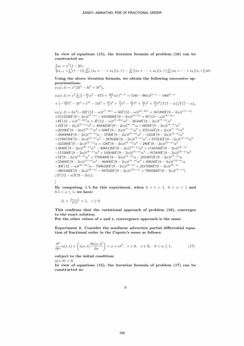
In view of equations (15), the iteration formula of problem (16) can beconstructed as:
ν0 = x2(1− 2t),
νk+1 =∫ t
0(τ − t)( ∂α
∂τα (ν0 + · · ·+ νk)(x, τ)− ∂∂x
[(ν0 + · · ·+ νk)(x, τ) ∂∂x
(ν0 + · · ·+ νk)(x, τ)])dτ.
Using the above iteration formula, we obtain the following successive ap-proximations:ν1(x, t) = x2(2t4 − 4t3 + 3t2),
ν2(x, t) = x2 415
[(− 45
2α2 − 675 + 495
2α)t4−α + (540− 90α)t5−α − 180t6−α
+(− 120
7t7 − 5t9 + t10 − 15t3 + 87
4t6 + 75
4t4 − 45
2t5 + 45
4t2 + 45
4t8
)Γ(7− α)]/Γ(7− α),
ν3(x, t) = 6x2(−32Γ(12− α)t(7−2α) + 56Γ(12− α)t(6−2α) + 161280Γ(9− 2α)t(11−α)
+5512320Γ(9− 2α)t(7−α) − 8316000Γ(9− 2α)t(4−α) + 8Γ(12− α)t(8−2α)
+8Γ(12− α)t(7−2α)α + 4Γ(12− α)t(6−2α)α2 − 26448Γ(9− 2α)t(7−α)α3
+24Γ(9− 2α)t(5−α)α6 + 4044032Γ(9− 2α)t(6−α)α + 6650Γ(9− 2α)t(4−α)α5
+20160Γ(9− 2α)t(9−α)α2 + 696Γ(9− 2α)t(7−α)α4 + 375144Γ(9− 2α)t(7−α)α2
−5880096Γ(9− 2α)t(5−α)α− 5760Γ(9− 2α)t(6−α)α4 − 1224Γ(9− 2α)t(5−α)α5
+1788576Γ(9− 2α)t(5−α)α2 − 287640Γ(9− 2α)t(5−α)α3 + 672245Γ(9− 2α)t(4−α)α3
−423360Γ(9− 2α)t(9−α)α + 128Γ(9− 2α)t(6−α)α5 − 280Γ(9− 2α)t(4−α)α6
+3840Γ(9− 2α)t(8−α)α3 − 3088120Γ(9− 2α)t(4−α)α2 + 1148160Γ(9− 2α)t(8−α)
−115200Γ(9− 2α)t(8−α)α2 + 103040Γ(9− 2α)t(6−α)α3 − 915840Γ(9− 2α)t(6−α)α2
+5Γ(9− 2α)t(4−α)α7 + 7788300Γ(9− 2α)t(4−α)α− 2353872Γ(9− 2α)t(7−α)α+25800Γ(9− 2α)t(5−α)α4 − 86800Γ(9− 2α)t(4−α)α4 + 80640Γ(9− 2α)t(10−α)α−30Γ(12− α)t(6−2α)α− 7096320Γ(9− 2α)t(6−α) + 2217600Γ(9− 2α)t(9−α)
−3801600Γ(9− 2α)t(8−α) − 887040Γ(9− 2α)t(10−α) + 7983360Γ(9− 2α)t(5−α))/(Γ(12− α)Γ(9− 2α)),...By computing βi’s for this experiment, when 0 < t < 1, 0 < x < 1 and0.5 < α ≤ 1, we have:
βi =‖νi+1‖‖νi‖ < 1, i ≥ 0.
This confirms that the variational approach of problem (16), convergesto the exact solution.For the other values of x and t, convergence approach is the same.
Experiment 2. Consider the nonlinear advection partial differential equa-tion of fractional order in the Caputo’s sense as follows:
∂α
∂tαu(x, t) +
(u(x, t)
∂u(x, t)
∂x
)= x + xt2, t > 0, x ∈ R, 0 < α ≤ 1, (17)
subject to the initial condition:u(x, 0) = 0.In view of equations (15), the iteration formula of problem (17) can beconstructed as:
9
ZANDY, AMINATAEI: PDE OF FRACTIONAL ORDER
165

ν0 = 0,
νk+1 = − ∫ t
0( ∂α
∂τα (ν0 + · · ·+ νk)(x, τ) + [(ν0 + · · ·+ νk)(x, τ) ∂∂x
(ν0 + · · ·+ νk)(x, τ)]− x− xτ2)dτ.
Using the above iteration formula, we obtain the following successive ap-proximations:
ν1(x, t) = x(t + t3
3),
ν2(x, t) = −x(
t2−α
Γ(3−α)+ 2t4−α
Γ(5−α)+ t7
63+ 2t5
15− t
),
ν3(x, t) = − 8x59535
[− 595352
((α− 3)(α− 5)2(−6 + α)2(α− 7)2(α− 8)2(α− 4)2Γ(7− 2α)
−8(α− 52)Γ(9− α)2)(α− 10)(α− 3)(α− 12)(α− 9
2)(α− 7
2)t(5−2α) + (α− 5
2)
(−119070Γ(7− 2α)(α− 10)(α− 8)2(α− 3)(α− 7)2(α− 12)(α− 92)(α− 4)(α− 5)2
(α− 6)2t(7−2α) + (−119070Γ(7− 2α)(α− 10)(α− 12)(α− 5)2(α− 6)2(α− 7)2(α− 8)2
t(9−2α)+(119070Γ(7−2α)(α−12)(α−3)(α−4)(α−5)(α−6)(α−7)(α−8)(α−10)t(2−α)
−1890Γ(7− 2α)(α− 8)(α− 7)(α− 12)(α2 − 7α + 1445
)(α− 5)(α− 6)t(10−α)
238140(α− 52)Γ(7− 2α)(α− 8)(α− 7)(α− 12)(α− 5)(α− 6)t(4−α)
+39690Γ(7− 2α)(α− 12)(α− 7)(α− 8)(α3 − 12α + 59α− 144)t(6−α)
−15876Γ(7− 2α)(α− 12)(α5 − 25α4 + 240α3 − 1085α2 + 2219α− 1170)t(8−α)
−3780Γ(7−2α)(α−5)(α−6)(α−7)(α−8)t(12−α)+(476280(α− 52)(α−3)(α−2)t(3−2α)
+Γ(7− 2α)t(t14 + 25213
t12 + 15876t4 + 214255
t10 − 1008t8 − 3591t6 + 59535t2 − 59535))Γ(9− α)(α− 12))(α− 10))Γ(9− α)(α− 9
2))(α− 7
2))]/
((α− 10)(α− 12)Γ(9− α)2(2α + 5)(2α− 9)(2α− 7)Γ(7− 2α)),...By computing βi’s for this experiment, when 0 < t < 1, 0 < x < 1 and0.5 < α ≤ 1, we have:
βi =‖νi+1‖‖νi‖ < 1, i ≥ 0.
This confirms that the variational approach of problem (17), convergesto the exact solution.For the other values of x and t, convergence approach is the same.
7 Conclusion
There are two main goals that we aimed in this paper. The first ispresenting an alternative approach of the variational iteration method tohandle nonlinear partial differential equations with fractional derivative inthe Caputo’s sense. The second is studying the convergence analysis andaddressing the sufficient condition for convergence. These two goals areachieved. We have studied the convergence of the presented approach andthe main results are given in theorems 1-3. Furthermore, we have exam-ined the convergence condition of VIM solution for the nonlinear problems.The VIM gives several successive approximations through using the iter-ation of the correction functional without any restrictive assumptions ortransformation and hence the procedure is direct and straightforward. TheVIM proved to be easy to use and provides an efficient method for handlingnonlinear problems, where a few approximation can be used to achieve thehigher order accuracy. Moreover, VIM reduces the size of calculations and
10
ZANDY, AMINATAEI: PDE OF FRACTIONAL ORDER
166

facilitates the computational work when compared with Adomian decom-position method or perturbation techniques.
References
[1] J. H. He, Approximate solution of nonlinear differential equations withconvolution product nonlinearities, Comput. Methods Appl. Mech.Eng., 167,69-73(1998).
[2] J. H. He, Approximate analytical solution for seepage flow with frac-tional derivatives in porous media, Comput. Methods Appl. Mech.Eng., 167, 57-68(1998).
[3] J. H. He, Variational iteration method- a kind of nonlinear analyt-ical technique: Some examples, Int. J. Nonlinear Mech., 34, 699-708(1999).
[4] J. H. He, Variational iteration method for autonomous ordinary dif-ferential systems, Appl. Math. Comput., 114, 115-123(2000).
[5] J. H. He, Variational principles for some nonlinear partial differentialequations with variable coefficients, Chaos, Solitons & Fractals, 19,847-851(2004).
[6] J. H. He, Some asymptotic methods for strongly nonlinear equations,Inter. J. Modern Phys. B, 20, 1141-1199(2006).
[7] J. H. He, Variational iteration method- some recent results and newinterpretations, J. Comput. Appl. Math., 207, 3-17(2007).
[8] J. H. He and X. H. Wu, Variational iteration method: New develop-ment and applications, J. Appl. Comput. Math., 54, 881-894(2007).
[9] M. A. Abdou and A. A. Soliman, Variational iteration method forsolving burger’s and coupled Burger’s equations, J. Appl. Comput.Math., 181, 245-251(2005).
[10] E. M. Abulwafa , M. A. Abdou and A. A. Mahmoud, The solutionof nonlinear coagulation problem with mass loss, Chaos, Solitons &Fractals, 29, 313-330(2006).
[11] S. Momani and Z. Odibat, Analytical approach to linear fractionalpartial differential equation arising in fluid mechanics, Phys. Lett. A,355, 271-279(2006).
[12] A. M. Wazwaz, A comparison between the variational iterationmethod and Adomian decomposition method, J. Appl. Comput.Math., 207, 129-136(2007).
[13] A. M. Wazwaz, The variational iteration method : A reliable tool forsolving linear and nonlinear wave equations, J. Comput. Math. Appl.,54,926-932(2007).
[14] A. M. Wazwaz, The variational iteration method for solving linearand nonlinear systems of PDEs, J. Appl. Comput. Math., 54, 895-902(2007).
11
ZANDY, AMINATAEI: PDE OF FRACTIONAL ORDER
167

[15] A. M. Wazwaz, The variational iteration method: A powerful schemefor handling linear and nonlinear diffusion equations, J. Appl. Com-put. Math., 54, 933-939(2007).
[16] A. M. Wazwaz, The variational iteration method for analytic treat-ment for linear and nonlinear ODEs, J. Appl. Comput. Math., 212,120-134(2009).
[17] S. Momani and S. Abuasad, Application of He’s variational iterationmethod to Helmholtz equation, Chaos, Solitons & Fractals, 27, 1119-1123(2006).
[18] M. A. Abdou and A. A. Soliman, New applications of variational it-eration method, Physica D, 211, 1-8(2005).
[19] J. H. He and X. H. Wu, Construction of solitary solution andcompacton-like solution by variational iteration method, Chaos, Soli-tons & Fractals, 29, 108-113(2006).
[20] M. Inc, Numerical simulation of kdv and mkdv equations with initialconditions by the variational iteration method, Chaos, Solitons &Fractals, 34, 1075-1081(2007).
[21] A. M. Wazwaz, The variational iteration method for rational solutionsfor kdv, k(2,2), Burgers, and cubic Boussinesq equations, J. Appl.Comput. Math., 207, 18-23(2007).
[22] M. A. Abdou and A. A. Soliman, Numerical solution of nonlinear evo-lution equations using variational iteration method, J. Appl. Comput.Math., 207 111-120(2007).
[23] Z. Odibat, Construction of solitary for nonlinear dispersive equationsby variational iteration method, Phys. Lett. A, 372, 4045-4052(2008).
[24] Z. Odibat and S. Momani, Application of variational iteration methodto nonlinear differential equations of fractional order, Inter. J. Non-linear Sci. Numer. Simul., 7, 27-34(2006).
[25] S. Abbasbandy, Approximation solution of a nonlinear equation withRiemann-Liouville’s fractional derivatives by He’s variational iterationmethod, J. Appl. Comput. Math., 207, 53-58(2007).
[26] Z. Odibat and S. Momani, Numerical comparison of methods for solv-ing linear differential equations of fractional order, Chaos, Solitons &Fractals, 31, 1248-1255(2007).
[27] Z. Odibat and S. Momani, Numerical approach to differential equa-tions of fractional order, J. Appl. Comput. Math., 207, 96-110(2007).
[28] Z. Odibat and S. Momani, Comparison between homotopy pertur-bation method and the variational iteration method for linear frac-tional partial differential equations, J. Appl. Comput. Math., 54,910-919(2007).
[29] Z. Odibat and S. Momani, Numerical methods for solving nonlinearpartial differential equations of fractional order, J. Appl. Comput.Math., 32, 28-39(2008).
12
ZANDY, AMINATAEI: PDE OF FRACTIONAL ORDER
168

[30] Z. Odibat and S. Momani, Applications of variational iteration andhomotopy perturbation methods to fractional evolution equations,Topol. Methods Nonlinear Anal., 31, 227-234(2008).
[31] Z. Odibat and S. Momani, Analytical comparison between the ho-motopy perturbation and variational iteration method for differen-tial equations of fractional order, Inter. J. Modern Phys. B, 22, 1-18(2008).
[32] S. Das, Solution of fractional vibration equation by the variationaliteration method and modified decomposition method, Inter. J. Non-linear Sci. Numer. Simul., 9, 361-366(2008).
[33] S. Das, Analytical solution of a fractional diffusion equation by varia-tional iteration method, J. Appl. Comput. Math., 57, 361-366(2009).
[34] Z. Odibat and S. Momani, The variational iteration method: An ef-ficient scheme for handling fractional partial differential equations influid mechanics, J. Appl. Comput. Math., 58, 2199-2208(2009).
[35] G. E. Draganescu and V. Capalnasan, Nonlinear relaxation phenom-ena in polycrystalline solids, Inter. J. Nonlinear Sci. Numer. Simul.,4, 219-225(2003).
[36] M. D’Acunto, Self-excited systems: Analytical determination of limitcycles, Chaos, Solitons & Fractals, 30, 719-724(2006).
[37] E. M. Abulwafa, M. A. Abdou and A. A. Mahmoud, Nonlinear fluidflows in pipe-like domain problem using variational iteration method,Chaos, Solitons & Fractals, 32, 1384-1397(2007).
[38] L. Xu, He’s parameter-expanding methods for strongly nonlinear os-cillators, J. Appl. Comput. Math., 207, 148-154(2007).
[39] D. D. Ganji and A. sadighi, Application of homotopy perturbation andvariational iteration methods to nonlinear heat transfer and porousmedia equations, J. Appl. Comput. Math., 207, 24-34(2007).
[40] N. H. Sweilam and M. M. Khader, Variational iteration method for onedimentional nonlinear thermoelasticity, Chaos, Solitons & Fractals,33, 145-149(2007).
[41] Z. M. Odibat, A study on the convergence of He’s variational iterationmethod, Math. & Comput. Modelling, preprint(2010).
[42] I. Podlubny, Fractional Differential Equations, Academic Press, NewYork(1999).
[43] R. Gorenflo and F. Mainardi, Fractional calculus: Integral and differ-ential equations of fractional order, in: Carpinteri, Mainardi (Eds),Fractals and Fractional Calculus, New York(1997).
[44] M. Caputo, Linear models of dissipation whose Q is almost frequencyindependent, Part 2, J. R. Astron. Soc: 13, 529-539(1967).
[45] M. Tatari and M. Dehghan, He’s variational iteration method for com-puting a control parameter in a semi-linear inverse parabolic equation,Chaos, Solitons & Fractals, 33, 671-677(2007).
[46] M. Tatari and M. Dehghan, On the convergence of He’s variationaliteration method, J. Appl. Comput. Math., 207, 121-128(2008).
13
ZANDY, AMINATAEI: PDE OF FRACTIONAL ORDER
169

JAFA
LATTICTIC RANDOM STABILITY OF AN ADDITIVE-QUADRATICFUNCTIONAL EQUATION BY FIXED POINT METHOD
CHOONKIL PARK AND REZA SAADATI∗
Abstract. In [39], Th.M. Rassias proved that the norm defined over a real vector space
V is induced by an inner product if and only if for a fixed positive integer l
2l
∥∥∥∥∥1
2l
2l∑i=1
xi
∥∥∥∥∥
2
+
2l∑i=1
∥∥∥∥∥xi − 1
2l
2l∑j=1
xj
∥∥∥∥∥
2
=
2l∑i=1
‖xi‖2
holds for all x1, · · · , x2l ∈ V . For the above equality, we can define the following func-
tional equation
2lf
(1
2l
2l∑i=1
xi
)+
2l∑i=1
f
(xi − 1
2l
2l∑j=1
xj
)=
2l∑i=1
f(xi). (1)
Using the fixed point method, we prove the generalized Hyers-Ulam stability of the
functional equation (1) in complete lattictic random normed spaces.
1. Introduction
Probability theory is a powerful hand set for modeling uncertainty and vagueness in
various problems arising in the field of science and engineering. It has also very useful
applications in various fields, e.g. population dynamics, chaos control, computer program-
ming, nonlinear dynamical systems, nonlinear operators, statistical convergence, etc. The
random topology proves to be a very useful tool to deal with such situations where the use
of classical theories breaks down. The usual uncertainty principle of Werner Heisenberg
leads to a generalized uncertainty principle, which has been motivated by string theory
and non-commutative geometry. In strong quantum gravity regime space-time points
are determined in a random manner. Thus impossibility of determining the position of
particles gives the space-time a random structure. Because of this random structure, posi-
tion space representation of quantum mechanics breaks down and therefore a generalized
normed space of quasi-position eigenfunction is required. Hence, one needs to discuss on
a new family of random norms. There are many situations where the norm of a vector is
not possible to be found and the concept of random norm seems to be more suitable in
2000 Mathematics Subject Classification. Primary 54E40; Secondary 39B82, 46S50, 46S40.
Key words and phrases. Stability; Random normed space; fixed point; generalized Hyers-Ulam stability;
fixed point, functional equation related to inner product space; quadratic mapping; additive mapping;
Lattice.0The corresponding author: [email protected] (Reza Saadati)
1
170
JOURNAL OF APPLIED FUNCTIONAL ANALYSIS, VOL.7, NO’S 1-2,170-184,COPYRIGHT 2012 EUDOXUS PRESS,LLC
2 PARK AND SAADATI
such cases, that is, we can deal with such situations by modeling the inexactness through
the random norm.
The stability problem of functional equations was originated from a question of Ulam
[52] concerning the stability of group homomorphisms. Hyers [15] gave a first affirmative
partial answer to the question of Ulam for Banach spaces. Hyers’ Theorem was generalized
by Aoki [2] for additive mappings and by Th.M. Rassias [38] for linear mappings by con-
sidering an unbounded Cauchy difference. The paper of Th.M. Rassias [38] has provided
a lot of influence in the development of what we call the generalized Hyers-Ulam stabil-
ity or the Hyers-Ulam-Rassias stability of functional equations. A generalization of the
Th.M. Rassias theorem was obtained by Gavruta [14] by replacing the unbounded Cauchy
difference by a general control function in the spirit of the Th.M. Rassias’ approach.
The functional equation
f(x + y) + f(x− y) = 2f(x) + 2f(y)
is called a quadratic functional equation. In particular, every solution of the quadratic
functional equation is said to be a quadratic mapping. A generalized Hyers-Ulam stabil-
ity problem for the quadratic functional equation was proved by Skof [51] for mappings
f : X → Y , where X is a normed space and Y is a Banach space. Cholewa [9] no-
ticed that the theorem of Skof is still true if the relevant domain X is replaced by an
Abelian group. Czerwik [10] proved the generalized Hyers-Ulam stability of the quadratic
functional equation. The stability problems of several functional equations have been
extensively investigated by a number of authors and there are many interesting results
concerning this problem (see [16], [18], [19], [35]–[37], [40]–[47]).
In [?], Park, Lee and Shin proved that an even mapping f : V → W satisfies the
functional equation (1) if and only if the even mapping f : V → W is quadratic. Moreover,
they proved the generalized Hyers-Ulam stability of the quadratic functional equation (1)
in real Banach spaces.
Let X be a set. A function d : X ×X → [0,∞] is called a generalized metric on X if d
satisfies
(1) d(x, y) = 0 if and only if x = y;
(2) d(x, y) = d(y, x) for all x, y ∈ X;
(3) d(x, z) ≤ d(x, y) + d(y, z) for all x, y, z ∈ X.
We recall a fundamental result in fixed point theory.
Theorem 1.1. [4, 12] Let (X, d) be a complete generalized metric space and let J : X → X
be a strictly contractive mapping with Lipschitz constant L < 1. Then for each given
element x ∈ X, either
d(Jnx, Jn+1x) = ∞for all nonnegative integers n or there exists a positive integer n0 such that
171

LATTICTIC RANDOM STABILITY OF AN AQ FUNCTIONAL EQUATION 3
(1) d(Jnx, Jn+1x) < ∞, ∀n ≥ n0;
(2) the sequence Jnx converges to a fixed point y∗ of J ;
(3) y∗ is the unique fixed point of J in the set Y = y ∈ X | d(Jn0x, y) < ∞; (4)
d(y, y∗) ≤ 11−Ld(y, Jy) for all y ∈ Y .
In 1996, G. Isac and Th.M. Rassias [17] were the first to provide applications of stability
theory of functional equations for the proof of new fixed point theorems with applications.
By using fixed point methods, the stability problems of several functional equations have
been extensively investigated by a number of authors (see [5], [6], [30], [32], [33], [34]).
2. Preliminaries
The theory of random normed spaces (RN-spaces) is important as a generalization of
deterministic result of linear normed spaces and also in the study of random operator
equations. The RN-spaces may also provide us the appropriate tools to study the ge-
ometry of nuclear physics and have important application in quantum particle physics.
The generalized Hyers-Ulam stability of different functional equations in random normed
spaces, RN-spaces and fuzzy normed spaces has been recently studied by Alsina [1], Mir-
mostafaee, Mirzavaziri and Moslehian [29, 30], Mihet and Radu [23], Mihet, Saadati and
Vaezpour [24, 25], Baktash et. al [3] and Saadati et. al. [48].
Let L = (L,≥L) be a complete lattice, i.e., a partially ordered set in which every
nonempty subset admits supremum and infimum, and 0L = inf L, 1L = supL. The space
of latticetic random distribution functions, denoted by ∆+L , is defined as the set of all
mappings F : R ∪ −∞,+∞ → L such that F is left continuous and non-decreasing on
R, F (0) = 0L, F (+∞) = 1L.
D+L ⊆ ∆+
L is defined as D+L = F ∈ ∆+
L : l−F (+∞) = 1L, where l−f(x) denotes the
left limit of the function f at the point x. The space ∆+L is partially ordered by the usual
point-wise ordering of functions, i.e., F ≥ G if and only if F (t) ≥L G(t) for all t in R. The
maximal element for ∆+L in this order is the distribution function given by
ε0(t) =
0L, if t ≤ 0,
1L, if t > 0.
Definition 2.1. ([8]) A triangular norm (t–norm) on L is a mapping T : (L)2 −→ L
satisfying the following conditions:
(a) (∀x ∈ L)(T (x, 1L) = x) (boundary condition);
(b) (∀(x, y) ∈ (L)2)(T (x, y) = T (y, x)) (commutativity);
(c) (∀(x, y, z) ∈ (L)3)(T (x, T (y, z)) = T (T (x, y), z)) (associativity);
(d) (∀(x, x′, y, y′) ∈ (L)4)(x ≤L x′ and y ≤L y′ =⇒ T (x, y) ≤L T (x′, y′)) (monotonic-
ity).
172

4 PARK AND SAADATI
Let xn be a sequence in L converges to x ∈ L (equipped order topology). The t-norm
T is said to be a continuous t–norm if
limn→∞ T (xn, y) = T (x, y),
for each y ∈ L.
Definition 2.2. ([8]) A continuous t–norm T on L = [0, 1]2 is said to be continuous t–
representable if there exist a continuous t–norm ∗ and a continuous t–conorm ¦ on [0, 1]
such that, for all x = (x1, x2), y = (y1, y2) ∈ L,
T (x, y) = (x1 ∗ y1, x2 ¦ y2).
For example,
T (a, b) = (a1b1,mina2 + b2, 1)and
M(a, b) = (mina1, b1,maxa2, b2)for all a = (a1, a2), b = (b1, b2) ∈ [0, 1]2 are continuous t–representable.
Define the mapping T∧ from L2 to L by:
T∧(x, y) =
x, if y ≥L x,
y, if x ≥L y.
Recall (see [20], [21]) that if xn is a given sequence in L, (T∧)ni=1xi is defined recurrently
by (T∧)1i=1xi = x1 and (T∧)ni=1xi = T∧((T∧)n−1
i=1 xi, xn) for n ≥ 2.
A negation on L is any decreasing mapping N : L → L satisfying N (0L) = 1L and
N (1L) = 0L. If N (N (x)) = x, for all x ∈ L, then N is called an involutive negation. In
the following L is endowed with a (fixed) negation N .
Definition 2.3. A latticetic random normed space is a triple (X,µ, T∧), where X is a
vector space and µ is a mapping from X into D+L such that the following conditions hold:
(LRN1) µx(t) = ε0(t) for all t > 0 if and only if x = 0;
(LRN2) µαx(t) = µx
(t|α|
)for all x in X, α 6= 0 and t ≥ 0;
(LRN3) µx+y(t + s) ≥L T∧(µx(t), µy(s)) for all x, y ∈ X and t, s ≥ 0.
We note that from (LRN2) it follows µ−x(t) = µx(t) (x ∈ X, t ≥ 0).
Example 2.4. Let L = [0, 1]× [0, 1] and operation ≤L be defined by:
L = (a1, a2) : (a1, a2) ∈ [0, 1]× [0, 1] and a1 + a2 ≤ 1,
(a1, a2) ≤L (b1, b2) ⇐⇒ a1 ≤ b1, a2 ≥ b2, ∀a = (a1, a2), b = (b1, b2) ∈ L.
Then (L,≤L) is a complete lattice (see [8]). In this complete lattice, we denote its
units by 0L = (0, 1) and 1L = (1, 0). Let (X, ‖ · ‖) be a normed space. Let T (a, b) =
173

LATTICTIC RANDOM STABILITY OF AN AQ FUNCTIONAL EQUATION 5
(mina1, b1,maxa2, b2) for all a = (a1, a2), b = (b1, b2) ∈ [0, 1] × [0, 1] and µ be a
mapping defined by
µx(t) =( t
t + ‖x‖ ,‖x‖
t + ‖x‖), ∀t ∈ R+, .
Then (X,µ, T ) is a latticetic random normed spaces.
If (X,µ, T∧) is a latticetic random normed space, then
V = V (ε, λ) : ε >L 0L, λ ∈ L \ 0L, 1L, V (ε, λ) = x ∈ X : Fx(ε) >L N (λ)
is a complete system of neighborhoods of null vector for a linear topology on X generated
by the norm F .
Definition 2.5. Let (X,µ, T∧) be a latticetic random normed spaces.
(1) A sequence xn in X is said to be convergent to x in X if, for every t > 0 and
ε ∈ L \ 0L, there exists a positive integer N such that µxn−x(t) >L N (ε) whenever
n ≥ N .
(2) A sequence xn in X is called Cauchy sequence if, for every t > 0 and ε ∈ L\0L,there exists a positive integer N such that µxn−xm(t) >L N (ε) whenever n ≥ m ≥ N .
(3) A latticetic random normed spaces (X,µ, T∧) is said to be complete if and only if
every Cauchy sequence in X is convergent to a point in X.
Theorem 2.6. If (X, µ, T∧) is a latticetic random normed space and xn is a sequence
such that xn → x, then limn→∞ µxn(t) = µx(t).
Proof. The proof is the same as classical random normed spaces, see [49]. ¤
3. Generalized Hyers-Ulam stability of the functional equation (1): an odd
case
For a given mapping f : X → Y , we define
Cf(x1, · · · , x2l) := 2lf
(12l
2l∑
i=1
xi
)+
2l∑
i=1
f
xi − 1
2l
2l∑
j=1
xj
−
2l∑
i=1
f(xi)
for all x1, · · · , x2l ∈ X.
Using the fixed point method, we prove the generalized Hyers-Ulam stability of the
functional equation Cf(x1, · · · , x2l) = 0 in complete LRN-space: an odd case.
Theorem 3.1. Let X be a linear space, (Y, µ, T∧) a complete LRN-space and Φ a mapping
from X2l to D+L (Φ(x1, ..., x2l) is denoted by Φx1,...,x2l
) and
Ψx := Φx, · · · , x︸ ︷︷ ︸l times
,0, · · · , 0︸ ︷︷ ︸l times
174

6 PARK AND SAADATI
be functions such that there exists an R < 1 with
Φx1,··· ,x2l
(R
2t
)≥L Φ2x1,··· ,2x2l
(t)
for all x1, · · · , x2l ∈ X. Let f : X → Y be an odd mapping satisfying
µCf(x1,··· ,x2l)(t) ≥L Φx1,··· ,x2l(t) (2)
for all x1, · · · , x2l ∈ X and all t > 0. Then A(x) := limn→∞ 2nf(
x2n
)exists for each
x ∈ X and defines an additive mapping A : X → Y such that
µf(x)−A(x)(t) ≥L Ψx((l − lR)t) (3)
for all x ∈ X and all t > 0.
Proof. Letting x1 = · · · = xl = x and xl+1 = · · · = x2l = 0 in (2), we get
µ2lf(x2 )−lf(x)(t) ≥L Φx, · · · , x︸ ︷︷ ︸
l times
,0, · · · , 0︸ ︷︷ ︸l times
(t) = Ψx(t) (4)
for all x ∈ X.
Consider the set
S := g : X → Y and introduce the generalized metric on S:
d(g, h) = infr ∈ R+ : µg(x)−h(x)(rt) ≥L Ψx(t), ∀x ∈ X, ∀t > 0,
where, as usual, inf ∅ = +∞. It is easy to show that (S, d) is complete. (See the proof of
Lemma 2.1 of [23].)
Now we consider the linear mapping J : S → S such that
Jg(x) := 2g(x
2
)
for all x ∈ X.
Let g, h ∈ S be given such that d(g, h) = ε. Then
µg(x)−h(x)(εt) ≥L Ψx(t)
for all x ∈ X and all t > 0. Hence
µJg(x)−Jh(x)(Rεt) = µ2g(x2 )−2h(x
2 )(Rεt)
= µg(x2 )−h(x
2 )
(R
2εt
)
≥L Ψx2
(Rt
2
)≥L Ψx
(Rt
2
)
= Ψx(t)
for all x ∈ X and all t > 0. So d(g, h) = ε implies that d(Jg, Jh) ≤ Rε. This means that
d(Jg, Jh) ≤ Rd(g, h)
175

LATTICTIC RANDOM STABILITY OF AN AQ FUNCTIONAL EQUATION 7
for all g, h ∈ S.
It follows from (4) that d(f, Jf) ≤ 1l .
By Theorem 1.1, there exists a mapping A : X → Y satisfying the following:
(i) A is a fixed point of J , i.e.,
A(x
2
)=
12A(x) (5)
for all x ∈ X. Since f : X → Y is odd, A : X → Y is an odd mapping. The mapping A is
a unique fixed point of J in the set
M = g ∈ S : d(f, g) < ∞.
This implies that A is a unique mapping satisfying (5) such that there exists a r ∈ (0,∞)
satisfying
µf(x)−A(x)(rt) ≥L Ψx(t)
for all x ∈ X;
(ii) d(Jnf,A) → 0 as n →∞. This implies the equality
limn→∞ 2nf
( x
2n
)= A(x)
for all x ∈ X;
(iii) d(f,A) ≤ 11−Rd(f, Jf), which implies the inequality
d(f, A) ≤ 1l − lR
.
This implies that the inequality (2) holds.
By (1),
µ2nCf( x12n ,··· , x2l
2n )(2nt) ≥L Φ x1
2n ,··· , x2l2n
(t)
for all x1, · · · , x2l ∈ X, all t > 0 and all n ∈ N. So
µ2nCf( x12n ,··· , x2l
2n )(t) ≥L Φx1,··· ,x2l
(t
Rn
)
for all x1, · · · , x2l ∈ X, all t > 0 and all n ∈ N. Since
limn→∞Φx1,··· ,x2l
(t
Rn
)= 1L
for all x1, · · · , x2l ∈ X and all t > 0,
µCA(x1,··· ,x2l)(t) = 1L
for all x1, · · · , x2l ∈ X and all t > 0. Thus CA(x1, · · · , x2l) = 0. Since A is odd, it follows
from Lemma 2.1 of [?] that the mapping A : X → Y is additive, as desired. ¤
176
8 PARK AND SAADATI
Corollary 3.2. Let θ ≥ 0 and let p be a real number with p > 1. Let X be a normed
vector space with norm ‖ · ‖ and let (X, µ,min) be a a complete LRN-space in which µ is
a distribution function on D+[0,1] = D+ i.e., L = [0, 1] (see [49]). Let f : X → X be an odd
mapping satisfying
µCf(x1,··· ,x2l)(t) ≥t
t + θ∑2l
j=1 ‖xj‖p(6)
for all x1, · · · , x2l ∈ X and all t > 0. Then A(x) := limn→∞ 2nf(
x2n
)exists for each
x ∈ X and defines an additive mapping A : X → Y such that
µf(x)−A(x)(t) ≥(2p − 2)t
(2p − 2)t + 2pθ‖x‖p
for all x ∈ X and all t > 0.
Proof. The proof follows from Theorem 3.1 by taking
Φx1,··· ,x2l(t) :=
t
t + θ∑2l
j=1 ‖xj‖p
for all x1, · · · , x2l ∈ X. Then we can choose R = 21−p and we get the desired result. ¤
Theorem 3.3. Let X be a linear space, (Y, µ, T∧) a complete LRN-space and Φ a mapping
from X2l to D+L (Φ(x1, ..., x2l) is denoted by Φx1,...,x2l
) and
Ψx := Φx, · · · , x︸ ︷︷ ︸l times
,0, · · · , 0︸ ︷︷ ︸l times
be functions such that there exists an R < 1 with
Φx1,··· ,x2l(2Rt) ≥L Φx1
2,··· , x2l
2(t)
for all x1, · · · , x2l ∈ X. Let f : X → Y be an odd mapping satisfying
µCf(x1,··· ,x2l)(t) ≥L Φx1,··· ,x2l(t) (7)
for all x1, · · · , x2l ∈ X and all t > 0. Then A(x) := limn→∞ 12n f(2nx) exists for each
x ∈ X and defines an additive mapping A : X → Y such that
µf(x)−A(x)(t) ≥L Ψx
((l − lR)
Rt
)(8)
for all x ∈ X and all t > 0.
Proof. Let (S, d) be the generalized metric space defined in the proof of Theorem 3.1.
Consider the linear mapping J : S → S such that
Jg(x) :=12g (2x)
for all x ∈ X.
It follows from (7) that
µ2lf(x)−lf(2x)(t) ≥L Ψ2x(t)
177
LATTICTIC RANDOM STABILITY OF AN AQ FUNCTIONAL EQUATION 9
for all x ∈ X and all t > 0. Thus
µf(x)− 12f(2x)
(2R
2lt
)≥L Ψx(t)
for all x ∈ X and all t > 0. So d(f, Jf) ≤ Rl .
The rest of the proof is similar to the proof of Theorem 3.1. ¤
Corollary 3.4. Let θ ≥ 0 and let p be a real number with 0 < p < 1. Let X be a normed
vector space with norm ‖ · ‖ and let (X, µ,min) be a a complete LRN-space in which µ is
a distribution function on D+[0,1] = D+ i.e., L = [0, 1] (see [49]). Let f : X → X be an
odd mapping satisfying (6). Then A(x) := limn→∞ 12n f (2nx) exists for each x ∈ X and
defines an additive mapping A : X → X such that
µf(x)−A(x)(t) ≥(2− 2p)t
(2− 2p)t + 2pθ‖x‖p
for all x ∈ X and all t > 0.
Proof. The proof follows from Theorem 3.3 by taking
Φx1,··· ,x2l(t) :=
t
t + θ∑2l
j=1 ‖xj‖p
for all x1, · · · , x2l ∈ X. Then we can choose R = 2p−1 and we get the desired result. ¤
4. Generalized Hyers-Ulam stability of the functional equation (1): an even
case
In this section, using the fixed point method, we prove the generalized Hyers-Ulam
stability of the functional equation Cf(x1, · · · , x2l) = 0 in complete LRN-spaces: an even
case.
Theorem 4.1. Let X be a linear space, (Y, µ, T∧) a complete LRN-space and Φ a mapping
from X2l to D+L (Φ(x1, ..., x2l) is denoted by Φx1,...,x2l
) and
Ψx := Φx, · · · , x︸ ︷︷ ︸l times
,0, · · · , 0︸ ︷︷ ︸l times
be functions such that there exists an R < 1 with
Φx1,··· ,x2l
(R
4t
)≥L Φ2x1,··· ,2x2l
(t)
for all x1, · · · , x2l ∈ X. Let f : X → Y be an even mapping satisfying f(0) = 0 and (2).
Then Q(x) := limn→∞ 4nf(
x2n
)exists for each x ∈ X and defines a quadratic mapping
Q : X → Y such that
µf(x)−Q(x)(t) ≥L Ψx((l − lR)t) (9)
for all x ∈ X and all t > 0.
178
10 PARK AND SAADATI
Proof. Letting x1 = · · · = xl = x and xl+1 = · · · = x2l = 0 in (2), we get
µ4lf(x2 )−lf(x)(t) ≥L Φx, · · · , x︸ ︷︷ ︸
l times
,0, · · · , 0︸ ︷︷ ︸l times
(t) = Ψx(t) (10)
for all x ∈ X.
Let (S, d) be the generalized metric space defined in the proof of Theorem 3.1.
Now we consider the linear mapping J : S → S such that
Jg(x) := 4g(x
2
)
for all x ∈ X.
Let g, h ∈ S be given such that d(g, h) = ε. Then
µg(x)−h(x)(εt) ≥L Ψx(t)
for all x ∈ X and all t > 0. Hence
µJg(x)−Jh(x)(Rεt) = µ4g(x2 )−4h(x
2 )(Rεt)
= µg(x2 )−h(x
2 )
(R
4εt
)≥L Ψx
2
(Rt
4
)
≥L Ψx(t)
for all x ∈ X and all t > 0. So d(g, h) = ε implies that d(Jg, Jh) ≤ Rε. This means that
d(Jg, Jh) ≤ Rd(g, h)
for all g, h ∈ S.
It follows from (10) that d(f, Jf) ≤ 1l .
By Theorem 1.1, there exists a mapping Q : X → Y satisfying the following:
(i) Q is a fixed point of J , i.e.,
Q(x
2
)=
14Q(x) (11)
for all x ∈ X. Since f : X → Y is even, Q : X → Y is an even mapping. The mapping Q
is a unique fixed point of J in the set
M = g ∈ S : d(f, g) < ∞.
This implies that Q is a unique mapping satisfying (11) such that there exists a r ∈ (0,∞)
satisfying
µf(x)−Q(x)(rt) ≥L Ψx(t)
for all x ∈ X;
(ii) d(Jnf,Q) → 0 as n →∞. This implies the equality
limn→∞ 4nf
( x
2n
)= Q(x)
for all x ∈ X;
179

LATTICTIC RANDOM STABILITY OF AN AQ FUNCTIONAL EQUATION 11
(iii) d(f,Q) ≤ 11−Rd(f, Jf), which implies the inequality
d(f, Q) ≤ 1l − lR
.
This implies that the inequality (9) holds.
The rest of the proof is similar to the proof of Theorem 3.1. ¤
Corollary 4.2. Let θ ≥ 0 and let p be a real number with p > 2. Let Y be a normed
vector space with norm ‖ · ‖ and let (X, µ,min) be a a complete LRN-space in which µ is
a distribution function on D+[0,1] = D+ i.e., L = [0, 1] (see [49]). Let f : X → Y be an
even mapping satisfying f(0) = 0 and (6). Then Q(x) := limn→∞ 4nf(
x2n
)exists for each
x ∈ X and defines a quadratic mapping Q : X → Y such that
µf(x)−Q(x)(t) ≥(2p − 4)t
(2p − 4)t + 2pθ‖x‖p
for all x ∈ X and all t > 0.
Proof. The proof follows from Theorem 4.1 by taking
Φx1,··· ,x2l(t) :=
t
t + θ∑2l
j=1 ‖xj‖p
for all x1, · · · , x2l ∈ X. Then we can choose R = 22−p and we get the desired result. ¤
Similarly, we can obtain the following. We will omit the proof.
Theorem 4.3. Let X be a linear space, (Y, µ, T∧) a complete LRN-space and Φ a mapping
from X2l to D+L (Φ(x1, ..., x2l) is denoted by Φx1,...,x2l
) and
Ψx := Φx, · · · , x︸ ︷︷ ︸l times
,0, · · · , 0︸ ︷︷ ︸l times
be functions such that there exists an R < 1 with
Φx1,··· ,x2l(4Rt) ≥L Φx1
2,··· , x2l
2(t)
for all x1, · · · , x2l ∈ X. Let f : X → Y be an even mapping satisfying f(0) = 0 and (2).
Then Q(x) := limn→∞ 14n f (2nx) exists for each x ∈ X and defines a quadratic mapping
Q : X → Y such that
µf(x)−Q(x)(t) ≥L Ψx((l − lR)t)
for all x ∈ X and all t > 0.
Corollary 4.4. Let θ ≥ 0 and let p be a real number with 0 < p < 2. Let Y be a normed
vector space with norm ‖ · ‖ and let (X, µ,min) be a a complete LRN-space in which µ
is a distribution function on D+[0,1] = D+ i.e., L = [0, 1] (see [49]). Let f : X → Y be
180

12 PARK AND SAADATI
an even mapping satisfying f(0) = 0 and (6). Then Q(x) := limn→∞ 14n f (2nx) exists for
each x ∈ X and defines a quadratic mapping Q : X → Y such that
µf(x)−Q(x)(t) ≥(4− 2p)t
(4− 2p)t + 2pθ‖x‖p
for all x ∈ X and all t > 0.
Proof. The proof follows from Theorem 4.3 by taking
Φx1,··· ,x2l(t) :=
t
t + θ∑2l
j=1 ‖xj‖p
for all x1, · · · , x2l ∈ X. Then we can choose R = 2p−2 and we get the desired result. ¤
5. Conclusion
Remark 5.1. Let f : X → Y be an odd mapping for which there exists a function
ϕ : X2n → [0,∞) satisfying (2) in which
Φx1,··· ,x2n(t) :=t
t + ϕ(x1, · · · , x2n),
and
µx(t) =t
t + ‖x‖ .
By a similar method to the proof of Theorem 3.3, one can show that if there exists an
R < 1 such that
ϕ(x, · · · , x︸ ︷︷ ︸n times
, 0, · · · , 0︸ ︷︷ ︸n times
) ≤ 2Rϕ
x
2, · · · ,
x
2︸ ︷︷ ︸n times
, 0, · · · , 0︸ ︷︷ ︸n times
for all x ∈ X, then there exists a unique Jensen additive mapping A : X → Y satisfying
‖f(x)−A(x)‖ ≤ R
n− nRϕ(x, · · · , x︸ ︷︷ ︸
n times
, 0, · · · , 0︸ ︷︷ ︸n times
)
for all x ∈ X.
Remark 5.2. Let f : X → Y be an even mapping for which there exists a function
ϕ : X2n → [0,∞) satisfying (2) in which
Φx1,··· ,x2n(t) :=t
t + ϕ(x1, · · · , x2n),
µx(t) =t
t + ‖x‖ .
and f(0) = 0 such that∞∑
j=0
14j
ϕ(2jx1, · · · , 2jx2n) < ∞
181

LATTICTIC RANDOM STABILITY OF AN AQ FUNCTIONAL EQUATION 13
for all x1, · · · , x2n ∈ X. By a similar method to the proof of Theorem 4.3, one can show
that if there exists an R < 1 such that
ϕ(x, · · · , x︸ ︷︷ ︸n times
, 0, · · · , 0︸ ︷︷ ︸n times
) ≤ 4Rϕ
x
2, · · · ,
x
2︸ ︷︷ ︸n times
, 0, · · · , 0︸ ︷︷ ︸n times
for all x ∈ X, then there exists a unique Jensen type quadratic mapping Q : X → Y
satisfying
‖f(x)−Q(x)‖ ≤ R
n− nRϕ(x, · · · , x︸ ︷︷ ︸
n times
, 0, · · · , 0︸ ︷︷ ︸n times
)
for all x ∈ X.
Acknowledgement
The first author was supported by Basic Science Research Program through the Na-
tional Research Foundation of Korea funded by the Ministry of Education, Science and
Technology (NRF-2009-0070788).
References
[1] C. Alsina, On the stability of a functional equation arising in probabilistic normed spaces, in: General
Inequalities, vol. 5, Oberwolfach, 1986, Birkhauser, Basel, 1987, pp. 263–271.
[2] T. Aoki, On the stability of the linear transformation in Banach spaces, J. Math. Soc. Japan 2 (1950),
64–66.
[3] E. Baktash, Y.J. Cho, M. Jalili, R. Saadati and S.M. Vaezpour, On the stability of cubic mappings
and quadratic mappings in random normed spaces, J. Inequal. Appl. 2008, Art. ID 902187 (2008).
[4] L. Cadariu and V. Radu, Fixed points and the stability of Jensen’s functional equation, J. Inequal.
Pure Appl. Math. 4, no. 1, Art. ID 4 (2003).
[5] L. Cadariu and V. Radu, On the stability of the Cauchy functional equation: a fixed point approach,
Grazer Math. Ber. 346 (2004), 43–52.
[6] L. Cadariu and V. Radu, Fixed point methods for the generalized stability of functional equations in a
single variable, Fixed Point Theory and Applications 2008, Art. ID 749392 (2008).
[7] S.S. Chang, Y.J. Cho and S.M. Kang, Nonlinear Operator Theory in Probabilistic Metric Spaces,
Nova Science Publishers, Inc., New York, 2001.
[8] G. Deschrijver and E. E. Kerre. On the relationship between some extensions of fuzzy set theory,
Fuzzy Sets and Systems 23 (2003), 227–235.
[9] P.W. Cholewa, Remarks on the stability of functional equations, Aequationes Math. 27 (1984), 76–86.
[10] S. Czerwik, On the stability of the quadratic mapping in normed spaces, Abh. Math. Sem. Univ.
Hamburg 62 (1992), 59–64.
[11] P. Czerwik, Functional Equations and Inequalities in Several Variables, World Scientific Publishing
Company, New Jersey, Hong Kong, Singapore and London, 2002.
[12] J. Diaz and B. Margolis, A fixed point theorem of the alternative for contractions on a generalized
complete metric space, Bull. Amer. Math. Soc. 74 (1968), 305–309.
[13] Z. Gajda, On stability of additive mappings, Internat. J. Math. Math. Sci. 14 (1991), 431–434.
182
14 PARK AND SAADATI
[14] P. Gavruta, A generalization of the Hyers-Ulam-Rassias stability of approximately additive mappings,
J. Math. Anal. Appl. 184 (1994), 431–436.
[15] D.H. Hyers, On the stability of the linear functional equation, Proc. Nat. Acad. Sci. U.S.A. 27 (1941),
222–224.
[16] D.H. Hyers, G. Isac and Th.M. Rassias, Stability of Functional Equations in Several Variables,
Birkhauser, Basel, 1998.
[17] G. Isac and Th.M. Rassias, Stability of ψ-additive mappings: Appications to nonlinear analysis, In-
ternat. J. Math. Math. Sci. 19 (1996), 219–228.
[18] S. Jung, Hyers-Ulam-Rassias Stability of Functional Equations in Mathematical Analysis, Hadronic
Press lnc., Palm Harbor, Florida, 2001.
[19] S. Jung, Approximation of analytic functions by Hermite functions, Bull. Sci. Math. 133 (2009),
756–764.
[20] O. Hadzic and E. Pap, Fixed Point Theory in PM Spaces, Kluwer Academic Publishers, Dordrecht,
2001.
[21] O. Hadzic, E. Pap and M. Budincevic, Countable extension of triangular norms and their applications
to the fixed point theory in probabilistic metric spaces, Kybernetica 38 (2002), 363–381.
[22] D. Mihet, The fixed point method for fuzzy stability of the Jensen functional equation, Fuzzy Sets and
Systems 160 (2009), 1663–1667.
[23] D. Mihet and V. Radu, On the stability of the additive Cauchy functional equation in random normed
spaces, J. Math. Anal. Appl. 343 (2008), 567–572.
[24] D. Mihet, R. Saadati and S.M. Vaezpour, The stability of the quartic functional equation in random
normed spaces, Acta Appl. Math. 110 (2010), 797–803.
[25] D. Mihet, R. Saadati and S.M. Vaezpour, The stability of an additive functional equation in Menger
probabilistic ϕ-normed spaces, Math. Slovak (in press).
[26] A.K. Mirmostafaee, A fixed point approach to almost quartic mappings in quasi fuzzy normed spaces,
Fuzzy Sets and Systems 160 (2009), 1653–1662.
[27] A.K. Mirmostafaee, M. Mirzavaziri and M.S. Moslehian, Fuzzy stability of the Jensen functional equa-
tion, Fuzzy Sets and Systems 159 (2008), 730–738.
[28] A.K. Mirmostafaee and M.S. Moslehian, Fuzzy versions of Hyers-Ulam-Rassias theorem, Fuzzy Sets
and Systems 159 (2008), 720–729.
[29] A.K. Mirmostafaee and M.S. Moslehian, Fuzzy approximately cubic mappings, Inform. Sci. 178 (2008),
3791–3798.
[30] M. Mirzavaziri and M.S. Moslehian, A fixed point approach to stability of a quadratic equation, Bull.
Braz. Math. Soc. 37 (2006), 361–376.
[31] A.K. Mirmostafaee and M.S. Moslehian, Fuzzy stability of additive mappings in non-Archimedean
fuzzy normed spaces, Fuzzy Sets and Systems 160 (2009), 1643–1652.
[32] C. Park, Fixed points and Hyers-Ulam-Rassias stability of Cauchy-Jensen functional equations in
Banach algebras, Fixed Point Theory and Applications 2007, Art. ID 50175 (2007).
[33] C. Park, Generalized Hyers-Ulam-Rassias stability of quadratic functional equations: a fixed point
approach, Fixed Point Theory and Applications 2008, Art. ID 493751 (2008).
[34] V. Radu, The fixed point alternative and the stability of functional equations, Fixed Point Theory 4
(2003), 91–96.
[35] J.M. Rassias, On approximation of approximately linear mappings by linear mappings, Bull. Sci. Math.
108 (1984), 445–446.
[36] J.M. Rassias, Refined Hyers-Ulam approximation of approximately Jensen type mappings, Bull. Sci.
Math. 131 (2007), 89–98.
183
LATTICTIC RANDOM STABILITY OF AN AQ FUNCTIONAL EQUATION 15
[37] J.M. Rassias and M.J. Rassias, Asymptotic behavior of alternative Jensen and Jensen type functional
equations, Bull. Sci. Math. 129 (2005), 545–558.
[38] Th.M. Rassias, On the stability of the linear mapping in Banach spaces, Proc. Amer. Math. Soc. 72
(1978), 297–300.
[39] Th.M. Rassias, New characterizations of inner product spaces, Bull. Sci. Math. 108 (1984), 95–99.
[40] Th.M. Rassias, Problem 16; 2, Report of the 27th International Symp. on Functional Equations,
Aequationes Math. 39 (1990), 292–293; 309.
[41] Th.M. Rassias, On the stability of the quadratic functional equation and its applications, Studia Univ.
Babes-Bolyai XLIII (1998), 89–124.
[42] Th.M. Rassias, The problem of S.M. Ulam for approximately multiplicative mappings, J. Math. Anal.
Appl. 246 (2000), 352–378.
[43] Th.M. Rassias, On the stability of functional equations in Banach spaces, J. Math. Anal. Appl. 251
(2000), 264–284.
[44] Th.M. Rassias, On the stability of functional equations and a problem of Ulam, Acta Appl. Math. 62
(2000), 23–130.
[45] Th.M. Rassias and P. Semrl, On the behaviour of mappings which do not satisfy Hyers-Ulam stability,
Proc. Amer. Math. Soc. 114 (1992), 989–993.
[46] Th.M. Rassias and P. Semrl, On the Hyers-Ulam stability of linear mappings, J. Math. Anal. Appl.
173 (1993), 325–338.
[47] Th.M. Rassias and K. Shibata, Variational problem of some quadratic functionals in complex analysis,
J. Math. Anal. Appl. 228 (1998), 234–253.
[48] R. Saadati, S.M. Vaezpour and Y.J. Cho, A note on the ”On the stability of cubic mappings and
quadratic mappings in random normed spaces”, J. Inequal. Appl. 2009, Art. ID 214530 (2009)
[49] B. Schweizer and A. Sklar, Probabilistic Metric Spaces, Elsevier, North Holand, New York, 1983.
[50] A.N. Serstnev, On the notion of a random normed space, Dokl. Akad. Nauk SSSR 149 (1963) 280–283
(in Russian).
[51] F. Skof, Proprieta locali e approssimazione di operatori, Rend. Sem. Mat. Fis. Milano 53 (1983),
113–129.
[52] S. M. Ulam, A Collection of the Mathematical Problems, Interscience Publ. New York, 1960.
E-mail address: [email protected]
Choonkil Park
Department of Mathematics, Research Institute for Natural Sciences, Hanyang University,
Seoul 133-791, South Korea
Reza Saadati
Department of Mathematics, Science and Research Branch, Islamic Azad University, Tehran,
Iran.
E-mail address: [email protected]
184
ON mIg-NORMAL SPACES
HAINING LI AND ZHAOWEN LI
Abstract. In this paper, characterizations and properties of mIg-normal
space are given. Moreover, Urysohn’s Lemma on mIg-normal spaces is proved.
1. Introduction and preliminaries
Ideals were studied by Kuratowski [6] and Vaidyanathaswamy [15]. Their appli-cations have been researched intensively (see [2], [4]).
The concept of minimal spaces was introduced by Popa and Noiri [13], whichis a generalization of topological spaces. They given some characterizations andproperties of m-regular spaces and m-normal spaces. The concept of ideal minimalspaces was studied by Ozbakir and Yildirim [9]. They introduced mIg-closed setsin ideal minimal spaces and investigated some basic properties.
The purpose of this paper is to study separation properties in ideal minimalspaces. We introduce the concept of mIg-normal spaces and give their character-izations and properties. In addition, we prove Urysohn’s lemma on mIg-normalspaces.
Throughout this paper, spaces always mean minimal spaces or ideal minimalspaces on which no separation axiom is assumed, and maps are onto. N denotesthe set of all natural integers. 2X denotes the power set of X. If U ⊂ 2X , Y ⊂ Xand x ∈ X, UY denotes U ⋂
Y : U ∈ U, U(x) denotes U ∈ U : x ∈ U, Uc
denotes X − U : U ∈ U.2. Preliminaries
Let X be a set and I,M ⊂ 2X . I is called an ideal on X if I satisfies thefollowing conditions:
(1) A ∈ I and B ⊂ A implies B ∈ I;(2) A ∈ I and B ∈ I implies A ∪B ∈ I.
M is called a minimal structure on X if ∅, X ∈ M. By (X,M), we denotea set X with a minimal structure M on X. Simply we call (X,M) a minimalspace (briefly m-space) [13]. Elements in M are called m-open subsets and thecomplements are called m-closed subsets.
Let (X,M) be a m-space. For A ⊂ X, the m-closure of A and the m-interior ofA are defined as the following [6]:
intm(A) =⋃U : U ⊂ A,U ∈M,
2000 Mathematics Subject Classification. 54A05, 54C08.Key words and phrases. Ideal m-spaces; mIg-closed sets; mIg-normal spaces; Urysohn’s
lemma.This work is supported by the National Natural Science Foundation of China (No.11061004),
the Natural Science Foundation of Guangxi Province in China (No.2011GXNSFA018125) and the
Science Research Project of Guangxi University for Nationalities (No.2010ZD009).
1
185
JOURNAL OF APPLIED FUNCTIONAL ANALYSIS, VOL.7, NO’S 1-2,185-193,COPYRIGHT 2012 EUDOXUS PRESS,LLC

2 HAINING LI AND ZHAOWEN LI
clm(A) =⋂F : F ⊃ A,X − F ∈M.
Definition 2.1 ([3]). A m-space (X,M) is called having property [U ] if the unionof every subfamily of M belongs to M.
If I is an ideal on X and M is a minimal structure on X, then (X,M, I) iscalled an ideal m-space.
Let (X,M, I) be an ideal m-space. A set operator (.)∗ : 2X −→ 2X , called alocal map [1] of A with respect to M and I, is defined as follows: for any A ⊂ X,
A∗(I,M) = x ∈ X : V ∩A 6∈ I for every V ∈M(x).For A ⊂ X, the m-closure of A and the m-interior of A in X are defined as the
following [6]:cl∗m(A) = A ∪A∗(I,M),int∗m(A) = X − cl∗m(X −A).
When there is no chance for confusion, we will simply write imA for intm(A),cmA for clm(A), A∗ for A∗(I,M), i∗mA for int∗m(A) and c∗mA for cl∗m(A), respec-tively.
Lemma 2.2 ([3], [12]). Let (X,M) be a m-space and A,B ⊂ X. Then the followingproperties hold.
(1) If A ⊂ B, then cmA ⊂ cmB and imA ⊂ imB.(2) cm∅ = ∅, cmX = X, im∅ = ∅ and imX = X.(3) If A ∈M, then imA ⊂ A; if A ∈Mc, then A ⊂ cmA.(4) imimA = imA and cmcmA = cmA.(5) X − cmA = im(X −A) and X − imA = cm(X −A).(6) im(A ∩B) = imA ∩ imB and im(A ∪B) ⊃ imA ∪ imB.(7) cm(A ∪B) = cmA ∪ cmB and cm(A ∩B) ⊂ cmA ∩ cmB.(8) x ∈ clm(A) if and only if U ∩A 6= ∅ for every U ∈M(x).
Lemma 2.3 ([14]). Let (X,M) be a m-space and A ⊂ X, where (X,M) has theproperty [U ]. Then the following properties hold.
(1) imA = A if and only if A ∈M.(2) cmA = A if and only if A ∈Mc.(3) imA ∈M and cmA ∈Mc.
Definition 2.4 ([9]). Let (X,M) be a m-space and A ⊂ X. Then A is called(1) mg-closed in X if cmA ⊂ U whenever U is m-open and A ⊂ U .(2) mg-open in X if X −A is mg-closed in X.
Definition 2.5 ([9]). Let (X,M, I) be an ideal m-space and A ⊂ X. Then A iscalled
(1) m∗-closed in X if c∗mA = A, and m∗-open in X if X −A is m∗-closed in X.(2) mIg-closed in X if A∗m ⊂ U whenever U is m-open and A ⊂ U , and mIg-
open in X if X −A is mIg-closed in X.
Obviously, m-closed sets ⇒ m∗-closed sets andm-closed sets ⇒ mg-closed sets ⇒ mIg-closed sets ⇐ m∗-closed sets.
Definition 2.6. A function f : (X,M) → (Y,N ) is called(1) m-continuous [7] if f−1(V ) is m-open in X for each V ∈ N .(2) m-closed [11] if f(F ) is m-closed in Y for any X − F ∈M.
186
ON mIg-NORMAL SPACES 3
Definition 2.7 ([11]). A m-space (X,M) is called m-normal (resp. mg-normal)if for each pair consisting of disjoint m-closed subsets (resp. mg-closed subsets) Aand B, there exist disjoint m-open subsets U and V such that A ⊂ U and B ⊂ V .
3. On mIg-normal spaces
Definition 3.1. A ideal m-space (X,M, I) is called mIg-normal, if for each pairconsisting of disjoint mIg-closed subsets A and B, there exist disjoint m-open sub-sets U and V such that A ⊂ U and B ⊂ V .
Clearly, if I = ∅, then mIg-normal spaces and mg-normal spaces coincide.Every mIg-normal space is m-normal. But the following Example 3.2 illustrates
that m-normal spaces need not be mIg-normal.
Example 3.2. Let X = a, b, c, d, M = ∅, b, a, b, a, c, d, X and I =∅, a, c, a, c. Then Mc = ∅, b, c, d, a, c, d, X.
Pick A = b and B = c, d (resp. A = b and B = a, c, d), then there existdisjoint m-open subsets U = a, b and V = a, c, d such that A ⊂ U and B ⊂ V .Hence X be m-normal space.
Put C = b, c and D = a, d, then we have C∗m = b and D∗m = c, d. This
implies that C and D are disjoint mIg-closed subsets of X. But there not existsm-open subset containing C. Hence X be not mIg-normal space.
The following Theorem 3.3 gives some characterizations of mIg-normal spaces.
Theorem 3.3. Let (X,M, I) be an ideal m-space. Then the following are equiva-lent.
(1) X is mIg-normal;(2) For each mIg-closed subset A and mIg-open subset U containing A, there
exists m-open subset V containing A such that A ⊂ V ⊂ cmV ⊂ U ;(3) For each pair consisting of disjoint mIg-closed subsets A and B, there exists
m-open subsets U containing A such that cmU ∩B = ∅;(4) For each pair consisting of disjoint mIg-closed subsets A and B, there exist
a m-open subset U containing A and a m-open subset V containing B such thatcmU ∩ cmV = ∅.Proof. (1)⇒ (2). Let A be a mIg-closed set and U be a mIg-open set containingA. Then we have X − U is mIg-closed set and A ∩ (X − U) = ∅. Since X is amIg-normal space, then there exist disjoint m-open subsets U1 and V1 such thatA ⊂ U1 and X − U ⊂ V1. This implies that X − V1 ⊂ U . Since U1 ∩ V1 = ∅, thenwe obtain cmU1 ⊂ X − V1. Set V = U1, then cmV ⊂ X − V1 ⊂ U . Therefore,A ⊂ V ⊂ cmV ⊂ X − V1 ⊂ U .
(2)⇒ (3). Let A and B are disjoint mIg-closed subsets of X. Then we haveA ⊂ X−B and X−B is mIg-open. By (2), there exists m-open subset U containingA such that A ⊂ U ⊂ cmU ⊂ X −B. Therefore, cmU ∩B = ∅.
(3)⇒ (4). Let A and B are disjoint mIg-closed subsets of X. By (3), thereexists m-open subset U containing A such that cmU∩B = ∅. Since cmU is m-closedin X, then cmU is mIg-closed. By (3), there exists m-open subsets V containingB such that cmU ∩ cmV = ∅.
(4)⇒ (1). This is obvious. ¤
If I = ∅ in Theorem 3.3, then we have the following Corollary 3.4.
187
4 HAINING LI AND ZHAOWEN LI
Corollary 3.4. Let (X,M) be a m-space. Then the following are equivalent.(1) X is mg-normal;(2) For each mg-closed subset A and mg-open subset U containing A, there exists
m-open subset V containing A such that A ⊂ V ⊂ cmV ⊂ U ;(3) For each pair consisting of disjoint mg-closed subsets A and B, there exists
m-open subsets U containing A such that cmU ∩B = ∅;(4) For each pair consisting of disjoint mg-closed subsets A and B, there exist
a m-open subset U containing A and a m-open subset V containing B such thatcmU ∩ cmV = ∅.Lemma 3.5. Let (X,M, I) be a mIg-normal space. For each pair consisting ofdisjoint mIg-closed subsets A and B, there exist disjoint m-open subsets U and Vsuch that c∗mA ⊂ U and c∗mB ⊂ V .
Proof. Let A and B are disjoint mIg-closed subsets of X. By Theorem 3.3, thereexist a m-open subsets U containing A and a m-open subsets V containing B suchthat cmU ∩ cmV = ∅. Since A is mIg-closed, then we have A∗m ⊂ U . HenceA∗m ∪A = c∗mA ⊂ U . Similarly c∗mB ⊂ U . ¤
Theorem 3.6. Let (X,M, I) be a mIg-normal space. For each mIg-closed subsetA and mIg-open subset U containing A, there exists m-open subset V such thatA ⊂ c∗mA ⊂ V ⊂ i∗mU ⊂ U .
Proof. Let A be a mIg-closed and U be a mIg-open containing A in X. ThenA and X − U are disjoint mIg-closed in X. By Lemma 3.5, there exist disjointm-open subsets V1 and V2 such that c∗mA ⊂ V1 and c∗m(X−U) ⊂ V2. Thus we haveX − i∗mU = c∗m(X − U) ⊂ V2. Hence X − V2 ⊂ i∗mU . Since V1 ∩ V2 = ∅, then weobtain V1 ⊂ X − V2. Therefore, A ⊂ c∗mA ⊂ V1 ⊂ X − V2 ⊂ i∗mU ⊂ U . ¤
If I = ∅ in Theorem 3.6, then we have the following Corollary 3.7.
Corollary 3.7. Let (X,M) be a mg-normal space. For each mg-closed subsetA and mg-open subset U containing A, there exists m-open subset V such thatA ⊂ cmA ⊂ V ⊂ imU ⊂ U .
4. Properties of mIg-normal spaces
Recall that if I is an ideal of (X,M) and Y ⊂ X, then IY is an ideal of (Y,MY )(see [8]). So (Y,MY , IY ) is also an ideal m-space. Thus, (Y,MY , IY ) is called asubspace of (X,M, I).
Lemma 4.1. Let (X,M, I) be an ideal m-space and A ⊂ Y ⊂ X. Then
A∗m(IY ,MY ) = A∗m(I,M) ∩ Y.
Proof. Let y ∈ A∗m(I,M) ∩ Y , for every V ∈ MY (y). Then there exists U ∈ Msuch that V = U ∩ Y . Thus we have U ∈ M(y). This implies that U ∩ A 6∈ I.Since IY ⊂ I and U ∩ Y ∩ A = U ∩ A, then we obtain V ∩ A = U ∩ Y ∩ A 6∈ IY .Hence y ∈ A∗m(IY ,MY ) and A∗m(I,M) ∩ Y ⊂ A∗m(IY ,MY ).
Conversely. Since A∗m(IY ,MY ) = y ∈ Y : V ∩A 6∈ IY for every V ∈MY (y),then A∗m(IY , τY ) ⊂ Y . Let y ∈ A∗m(IY ,MY ), for every U ∈ M(y). Then U ∩ Y ∈MY (y). This implies that (U ∩ Y ) ∩A 6∈ IY . Since (U ∩ Y ) ∩A = U ∩A, then wehave U ∩A 6∈ I. Hence y ∈ A∗m(I,M) and A∗m(IY ,MY ) ⊂ A∗m(I,M) ∩ Y . ¤
188
ON mIg-NORMAL SPACES 5
Lemma 4.2. Let (X,M, I) be an ideal m-space and A ⊂ Y ⊂ X. If A is am(IY )g-closed subset of (Y,MY , IY ) and Y is m∗-closed in X, then A is a mIg-closed subset of (X,M, I).
Proof. Let A ⊂ U ∈ M, then A ⊂ U ∩ Y ∈ MY . Since A is m(IY )g-closed in Y ,then A∗m(IY ,MY ) ⊂ U ∩ Y . By Lemma 4.1, we have A∗m(I,M) ∩ Y ⊂ U ∩ Y .Since A ⊂ Y and Y is m∗-closed in X, then A∗m(I,M) ⊂ c∗mA ⊂ c∗mY = Y . Thuswe obtain A∗m(I,M) ⊂ U ∩ Y . Therefore A∗m(I,M) ⊂ U and A is mIg-closed inX. ¤
Theorem 4.3. Let (X,M, I) be a mIg-normal space and Y ⊂ X. If Y be am∗-closed subset of X, then (Y,MY , IY ) is a m(IY )g-normal space.
Proof. Let A and B are disjoint m(IY )g-closed subsets of Y . Since Y be a m∗-closedin X, then A and B are disjoint mIg-closed subsets of X by Lemma 4.2. Since(X,M, I) is mIg-normal space, then there exist disjoint m-open subsets U and Vsuch that A ⊂ U and B ⊂ V . Hence, A ⊂ U ∩ Y ∈ MY and B ⊂ V ∩ Y ∈ MY .Note that (U∩Y )∩(V ∩Y ) = ∅. Therefore (Y,MY ,J ) is m(IY )g-normal space. ¤
Lemma 4.4. Let (X,M, I) be an ideal m-space satisfying the property [U ] andB, Y ⊂ X. If B is a mIg-closed in X and Y is m-open and m-closed in X, thenB ∩ Y is a m(IY )g-closed subset of (Y,MY , IY ).
Proof. Let B ∩ Y ⊂ U ∈ MY , then B ⊂ U ∪ (X − Y ). U ∈ MY and Y ∈ Mimply U ∈ M. Since Y is also a m-closed in X, then U ∪ (X − Y ) ∈ M. SinceX has property [U ] and B is a mIg-closed in X, then B∗
m(I,M) ⊂ U ∪ (X − Y ).By Lemma 4.1, (B ∩ Y )∗m(IY ,MY ) = (B ∩ Y )∗m(I,M) ∩ Y ⊂ B∗
m(I,M) ∩ Y ⊂(U ∪ (X − Y )) ∩ Y = U . Therefore B ∩ Y is m(IY )g-closed in Y . ¤
Lemma 4.5 ([5]). If every Iα is an ideal of Xα, then ⋃α∈∧ Iα : Iα ∈ Iα is an
ideal of⋃
α∈∧ Xα.
Let (Xα,Mα) : α ∈ Λ be a family of pairwise disjoint m-space, i.e., Xα∩Xα′ =∅ for α 6= α′. Put X =
⋃α∈Λ
Xα, M = ⋃α∈Λ
Aα : Aα ∈ Mα. Obviously, ∅, X ∈ M.
So M is a minimal structure on X.For A ⊂ X, we claim A ∈ M if and only if A ∩ Xα ∈ Mα for each α ∈ ∧
.In fact. Suppose A ∈ M. Then A =
⋃β∈∧ Aβ , where Aβ ∈ Mβ (β ∈ Λ). So
for each α ∈ ∧, A ∩ Xα = (
⋃β∈∧ Aβ) ∩ Xα =
⋃β∈∧(Aβ ∩ Xα). If β 6= α, then
Aβ ∩ Xα ⊂ Xβ ∩ Xα = ∅. Thus A ∩ Xα = Aα ∩ Xα = Aα ∈ Mα. On the otherhand. A = A ∩ X = A ∩ (
⋃α∈∧ Xα) =
⋃α∈∧(A ∩ Xα). By A ∩ Xα ∈ Mα, A ∈ M.
Thus, the m-space (X,M) is called the mini sum of (Xα,Mα) : α ∈ Λ. Wedenote (X,M) by
⊕α∈∧ Xα.
It is easy to prove that every Xα are both m-open and m-closed in⊕
α∈∧ Xα.
Obviously, if every m-space (Xα,Mα) satisfies the property [U ], then⊕
α∈∧ Xα
also satisfies the property [U ].
189
6 HAINING LI AND ZHAOWEN LI
Let (Xα,Mα, Iα) : α ∈ ∧ be a family of pairwise disjoint ideal m-spaces,i.e., Xα ∩ Xα′ = ∅ for α 6= α′. Put X =
⋃α∈Λ
Xα, M = ⋃α∈Λ
Aα : Aα ∈ Mα,I = ⋃
α∈∧ Iα : Iα ∈ Iα. By Lemma 4.5, (X,M, I) is a ideal m-space. For A ⊂ X,
A ∈ M if and only if A ∩Xα ∈ Mα for each α ∈ ∧. Thus, 〈X,M, I〉 is called the
ideal mini sum of (Xα,Mα, Iα) : α ∈ Λ. We also denote (X,M, I) by⊕
α∈∧ Xα.
Theorem 4.6. Let (Xα,Mα, Iα) : α ∈ Λ be a family of pairwise disjoint idealm-spaces satisfying the property [U ] and let I = ⋃
α∈∧ Iα : Iα ∈ Iα. Then⊕
α∈∧ Xα
is a mIg-normal space if and only if every Xα is a m(Iα)g-normal space.
Proof. The proof of Necessity follows from Theorem 4.3.Sufficiency. Denote X =
⊕α∈∧ Xα.
Let A and B be disjoint mIg-closed subsets of X. Then for any α ∈ Λ, A ∩Xα
and B ∩ Xα are disjoint mIg-closed subsets of Xα by Lemma 4.4. Since Xα ism(Iα)g-normal, then there exist disjoint m-open subsets Uα and Vα of Xα suchthat A ∩Xα ⊂ Uα and B ∩Xα ⊂ Vα.
Clearly,A = A
⋂(
⋃α∈∧ Xα) ⊂ U =
⋃α∈∧ Uα,
B = B⋂
(⋃
α∈∧ Xα) ⊂ V =⋃
α∈∧ Vα.
If α 6= β, then Uα ∩ Vβ ⊂ Xα ∩ Xβ = ∅. Thus for any α, β ∈ Λ, Uα ∩ Vβ = ∅.Hence U
⋂V =
⋂α, β∈Λ
(Uα ∩ Vβ) = ∅.Since every Xα is m-open in X and X has property [U ], then U and V are
m-open in X. Therefore X is mIg-normal. ¤Lemma 4.7 ([10]). If f : X → Y is a map, A ⊂ X and B ⊂ Y , then f−1(B) ⊂ Aif and only if B ⊂ Y − f(X −A).
Lemma 4.8. Let f : (X,M, I) → (Y,N ,J ) be a map with f−1(J ) ⊂ I. Then(1) If f is a m-continuous map, then f−1(B)∗m(I,M) ⊂ f−1(B∗
m(J ,N )) forany B ⊂ Y .
(2) If f is a m-continuous and m-closed map and B is a mJg-closed subset ofY , then f−1(B) is a mIg-closed subset of X.
Proof. (1) Suppose that f(f−1(B)∗m(I,M))−B∗m(J ,N ) 6= ∅, pick
y ∈ f(f−1(B)∗m(I,M))−B∗m(J ,N ).
Thus we have y ∈ f(f−1(B)∗m(I,M)). This implies that y = f(x) for somex ∈ f−1(B)∗m(I,M). Since y 6∈ B∗
m(J ,N ), then V ∩ B ∈ J for some V ∈N (y). Since f is m-continuous, then f−1(V ) ∈ N (x). Thus f−1(V ) ∩ f−1(B) 6∈ I.But, V ∩ B ∈ J implies that f−1(V ) ∩ f−1(B) = f−1(V ∩ B) ∈ f−1(J ) ⊂ I.This is a contradiction. Hence f(f−1(B)∗m(I,M)) − B∗
m(J ,N ) = ∅. Therefore,f(f−1(B)∗m(I,M)) ⊂ B∗
m(J ,N ) and f−1(B)∗m(I,M) ⊂ f−1(B∗m(J ,N )).
(2) Let f−1(B) ⊂ U ∈ M, then B ⊂ Y − f(X − U) by Lemma 4.7. Since f ism-closed, then Y − f(X −U) ∈ N . Since B is mJg-closed in Y , then B∗
m(J ,N ) ⊂Y − f(X − U). By Lemma 4.7, f−1(B∗
m(J ,N )) ⊂ U . By (1), f−1(B)∗m(I,M) ⊂f−1(B∗
m(J ,N )). Hence f−1(B)∗m(I,M) ⊂ U . Therefore, f−1(B) is mIg-closed inX. ¤
190
ON mIg-NORMAL SPACES 7
Theorem 4.9. Let f : (X,M, I) → (Y,N ,J ) be a m-continuous and m-closedmap with f−1(J ) ⊂ I. If X is mIg-normal, then Y is mJg-normal.
Proof. Let A and B are disjoint mJg-closed subsets of Y , then f−1(A) and f−1(B)are disjoint mIg-closed subsets of X by Lemma 4.8. Since X is mIg-normal, thenexist disjoint m-open subsets U and V of X such that f−1(A) ⊂ U and f−1(B) ⊂ V .By Lemma 4.7, A ⊂ Y −f(X−U) and B ⊂ Y −f(X−V ). Note that Y −f(X−U)and Y − f(X − V ) are disjoint m-open subsets of Y . Hence Y is mJg-normal. ¤
If I = ∅ in Theorem 4.9, then we have the following Corollary 4.10.
Corollary 4.10. If X is mg-normal and f : (X,M) → (Y,N ) is a m-continuousand m-closed map, then Y is mg-normal.
5. Urysohn’s lemma on mIg-normal spaces.
Below we give Urysohn’s lemma on mIg-normal spaces.
Theorem 5.1. An ideal m-space (X,M, I) is mIg-normal if and only if for eachpair of disjoint mIg-closed subsets A and B of X, there exists a m-continuousmapping f : X → [0, 1] such that f(A) = 0 and f(B) = 1.Proof. Sufficiency. Suppose for each pair of disjoint mIg-closed subsets A and B ofX, there exists a m-continuous mapping f : X → [0, 1] such that f(A) = 0 andf(B) = 1. Put U = f−1([0, 1/2)), V = f−1((1/2, 1]), then U and V are disjointm-open subsets of X such that A ⊂ U and B ⊂ V . Hence X is mIg-normal.
Necessity. Suppose X is mIg-normal. For each pair of disjoint mIg-closedsubsets A and B of X, A ⊂ X − B, where A is mIg-closed and X − B in X ismIg-open in X. By Theorem 3.3, there exists an m-open subset U1/2 of X suchthat
A ⊂ U1/2 ⊂ cmU1/2 ⊂ X −B.Since A ⊂ U1/2, A is mIg-closed in X and U1/2 is mIg-open in X, then there
exists an m-open subset U1/4 of X such that A ⊂ U1/4 ⊂ cmU1/4 ⊂ U1/2 byTheorem 3.3. Since cmU1/2 ⊂ X − B, cmU1/2 is mIg-closed in X and X − B ismIg-open in X, then there exists an m-open subset U3/4 of X such that cmU1/2 ⊂U3/4 ⊂ cmU3/4 ⊂ X − B by Theorem 3.3. Thus, there exist two m-open subsetsU1/2 and U3/4 of X such that
A ⊂ U1/4 ⊂ cmU1/4 ⊂ U1/2 ⊂ cmU1/2 ⊂ U3/4 ⊂ cmU3/4 ⊂ X −B.We get a family Um/2n : 1 ≤ m < 2n, n ∈ N of m-open subsets of X, denotes
Um/2n : 1 ≤ m < 2n, n ∈ N by Uα : α ∈ Γ. Uα : α ∈ Γ satisfies the followingcondition:
(1) A ⊂ Uα ⊂ cmUα ⊂ X −B,(2) if α < α′, then cmUα ⊂ Uα′ .
We define f : X → [0, 1] as follows:
f(x) =
infα ∈ Γ : x ∈ Uα, if x ∈ Uα for some α ∈ Γ,1, if x 6∈ Uα for any α ∈ Γ.
For each x ∈ A, x ∈ Uα for any α ∈ Γ by (1), so f(x) = infα ∈ Γ : x ∈ Uα =infΓ = 0. Thus, f(A) = 0.
For each x ∈ B, x 6∈ X − B implies x 6∈ Uα for any α ∈ Γ by (1), so f(x) = 1.Thus, f(B) = 1.
We have to show f is m-continuous.
191

8 HAINING LI AND ZHAOWEN LI
For x ∈ X and α ∈ Γ, we have the following Claim:Claim 1: if f(x) < α , then x ∈ Uα.Suppose f(x) < α, then infα ∈ Γ : x ∈ Uα < α, so there exists α1 ∈ α ∈
Γ : x ∈ Uα such that α1 < α. By (2), cmUα1 ⊂ Uα.Notice that x ∈ Uα1 . Hencex ∈ Uα.
Claim 2: if f(x) > α , then x 6∈ cmUα.Suppose f(x) > α, then there exists α1 ∈ Γ such that α < α1 < f(x). Notice
that α1 ∈ α ∈ Γ : x ∈ Uα implies α1 ≥ infα ∈ Γ : x ∈ Uα = f(x). Thus,α1 6∈ α ∈ Γ : x ∈ Uα. So x 6∈ Uα1 . By (2), cmUα ⊂ Uα1 . Hence x 6∈ cmUα.
Claim 3: if x 6∈ cmUα, then f(x) ≥ α.Suppose x 6∈ cmUα, we claim that α < β for any β ∈ α ∈ Γ : x ∈ Uα.
Otherwise, there exists β ∈ α ∈ Γ : x ∈ Uα such that α ≥ β. x 6∈ cmUα
implies α 6∈ α ∈ Γ : x ∈ Uα. So α 6= β. Thus α > β. By (2), cUβ ⊂ Uα. Sox 6∈ β, contridiction. Therefore α < β for any β ∈ α ∈ Γ : x ∈ Uα. Henceα ≤ infα ∈ Γ : x ∈ Uα = f(x).
For x0 ∈ X, if f(x0) ∈ (0, 1), suppose V is an m-open neighborhood of f(x0)in [0, 1], then there exists ε > 0 such that (f(x0)− ε, f(x0) + ε) ⊂ V
⋂(0, 1). Pick
α′, α” ∈ Γ such that0 < f(x0)− ε < α′ < f(x0) < α” < f(x0) + ε < 1.
By Claim 1 and Claim 2, x0 ∈ Uα”, x0 6∈ cmU ′α. Put U = Uα”− cmU ′
α, thenU is an m-open neighborhood of x0 in X.
We will prove that f(U) ⊂ (f(x0) − ε, f(x0) + ε). if y ∈ f(U), then y = f(x)for some x ∈ U . x ∈ U implies that x ∈ Uα” and x 6∈ cmU ′
α. Since x ∈ Uα”, thenα” ∈ α ∈ Γ : x ∈ Uα. Thus, α” ≥ infα ∈ Γ : x ∈ Uα = f(x). Notice thatα” < f(x0) + ε. Therefore f(x) < f(x0) + ε. Since x 6∈ cmU ′
α, then f(x) ≥ α′
by Claim 3. Notice that f(x0) − ε < α′. Therefore f(x) > f(x0) − ε. Hence,f(U) ⊂ (f(x0)− ε, f(x0) + ε).
Therefore, f(U) ⊂ V . This implies f is m-continuous at x0.if f(x0) = 0, or 1, the proof that f is m-continuous at x0 is similar. ¤
If I = ∅ in Theorem 5.1, then we have the following Corollary 5.2.
Corollary 5.2. A m-space (X,M) is mg-normal if and only if for each pair ofdisjoint mg-closed subsets A and B of X, there exists a m-continuous mappingf : X → [0, 1] such that f(A) = 0 and f(B) = 1.
References
1. D.Jankovic and T.R.Hamlett, New topologies from old via ideals, Amer. Math. Monthly,97(1990), 295-310.
2. F.G.Arenas, J.Dontchev and M.L.Puertas, Idealization of some weak separation axioms. Acta
Math.Hungar., 89(1-2)(2000), 47-53.3. H. Maki, K.C.Rao, A. Nagoor Gani, On generalizing semi-open and preopen sets, Pure Appl.
Math. Sci., 49(1999), 17-29.4. J.Dontchev, M.Ganster and D. Rose, Ideal resolvability, TopologyAppl., 93(1999), 1-16.5. J.Dontchev, On Hausdorff spaces via topological ideals and I-irresolute functions, in: Papers
on General Topology and Applications, Ann. New York Acad. Sci., 767(1995), 28-38.6. K.Kuratowski, Topology, Academic press, New York, 1966.
7. M.Alimohammady, M.Roohi, Fixed point in minimal Spaces, Nonlinear Analysis: Modelling
and Control, 10(2005), 305-314.8. R.L.Newcomb, Topologies which are compact modulo an ideal, Ph.D. thesis, University of
Cal. at Santa Barbara, 1967.
192

ON mIg-NORMAL SPACES 9
9. O.B.Ozbakir, E.D.Yildirim, On some closed sets in ideal minimal spaces, Acta Math. Hungar.,
125(2009), 227-235.
10. S.Lin, Metric spaces and topology of funtion spaces, Chinese Scientific Publ., Beijing, 2004.11. T.Noiri, V.Popa, A unified theory of closed functions, Bull. Math. Soc. Sci. Math. Roumanie
Tome, 4(2006), 371-382.
12. V.Popa, T.Noiri, On m-continuous functions, Anal. Univ. ”Dunarea de Jos” Galati, Ser. Mat.Fiz. Mec. Teor., 18(2000), 31-41.
13. V.Popa, T.Noiri, On the definitions of some genralized forms of continuity under minimal
conditions, Mem. Fac. Sci. Kochi Univ. Ser. A, 22(2001), 9-18.14. V.Popa, T.Noiri, On weakly (τ, m)-continuous functions, Rend. Circ. Mat. Palermo, 51(2002),
295-316.15. R.Vaidyanathaswamy, The localization theory in set topology, Proc. Indian Acad. Sci.,
20(1944), 51-61.
College of Mathematics and Computer Science, Guangxi University for Nationali-
ties, Nanning, Guangxi 530006, P.R.ChinaE-mail address: [email protected]
College of Mathematics and Computer Science, Guangxi University for Nationali-ties, Nanning, Guangxi 530006, P.R.China
E-mail address: [email protected]
193

194

TABLE OF CONTENTS, JOURNAL OF APPLIED FUNCTIONAL
ANALYSIS, VOL. 7, NO.’S 1-2, 2012
Matrix–Valued Wavelets and Multiresolution Analysis, A. San Antolin and R. A. Zalik,…….…………………………………………………………………………………….13
The Random Motion on the Sphere Generated by the Laplace-Beltrami Operator, Dimitra Kouloumpou and Vassilis G. Papanicolaou,……….………………………………………… 26
Quantitative Estimates in the Overconvergence of Some Multivariate Singular Integrals, George A. Anastassiou and Sorin G. Gal,……………………………………………………………..42
A Note on Strong Differential Superordinations Using Sălăgean and Ruscheweyh Operators, Alina Alb Lupaş,……………………………………………………………………………...54
Certain Strong Differential Superordinations Using a Generalized Sălăgean Operator and Ruscheweyh Operator, Alina Alb Lupaş,……………………………………………………..62
A New Fixed Point Theorem for m Mapings On m Complete Metric Spaces, Luljeta Kikina and Kristaq Kikina,………………………………………………………………………………...69
Direct and Converse Theorems for Generalized Bernstein Polynomials Based on the q-Integers, İbrahim Büyükyazici,……………………………………………………………………….....81
A New Non-Unique Fixed Point Theorem, Erdal Karapinar,………………………………....92
A Simple Proof of the Nadler’s Contraction Principle, M. Eshaghi Gordji, H. Baghani and S. Davoudi,……………………………………………………………………………………......98
Some New Ostrowski Type Inequalities, W. T. Sulaiman,…………………………………...102
Logarithmic Order and Type on Some Weighted Function Spaces, A. El-Sayed Ahmed and A. Kamal,………………………………………………………………………………………...108
Some Fixed Point Theorem for Mapping on Complete G-Cone Metric Spaces, Duran Turkoglu and Nurcan Bilgili,…………………………………………………………………………....118
Stability of an Additive–Quadratic Functional Equation in Menger Probabilistic Normed Spaces, M. Eshaghi Gordji, M. Bavand Savadkouhi and S. M. Vaezpour,…………………………...138
On New Classes of Double Sequence Spaces Defined by Orlicz Function, Ayhan Esi,……..148
195
TABLE OF CONTENTS, JOURNAL OF APPLIED FUNCTIONAL
ANALYSIS, VOL. 7, NO.’S 1-2, 2012 (continued)
On the Convergence of Variational Iteration Method for the Solution of Partial Differential Equations of Fractional Order, M. Zandy and A. Aminataei,……………………………….157
Lattictic Random Stability of an Additive-Quadratic Functional Equation by Fixed Point Method, Choonkil Park and Reza Saadati,…………………………………………………..170
On mIg-Normal Spaces, Haining Li and Zhaowen Li,……………………………………….185
196
Volume 7, Number 3 July 2012 ISSN:1559-1948 (PRINT), 1559-1956 (ONLINE) EUDOXUS PRESS,LLC
JOURNAL OF APPLIED FUNCTIONAL ANALYSIS
197
SCOPE AND PRICES OF
JOURNAL OF APPLIED FUNCTIONAL ANALYSIS A quartely international publication of EUDOXUS PRESS,LLC ISSN:1559-1948(PRINT),1559-1956(ONLINE) Editor in Chief: George Anastassiou Department of Mathematical Sciences The University of Memphis Memphis, TN 38152,USA E mail: [email protected] Assistant to the Editor:Dr.Razvan Mezei,Lander University,SC 29649, USA. -------------------------------------------------------------------------------- The purpose of the "Journal of Applied Functional Analysis"(JAFA) is to publish high quality original research articles, survey articles and book reviews from all subareas of Applied Functional Analysis in the broadest form plus from its applications and its connections to other topics of Mathematical Sciences. A sample list of connected mathematical areas with this publication includes but is not restricted to: Approximation Theory, Inequalities, Probability in Analysis, Wavelet Theory, Neural Networks, Fractional Analysis, Applied Functional Analysis and Applications, Signal Theory, Computational Real and Complex Analysis and Measure Theory, Sampling Theory, Semigroups of Operators, Positive Operators, ODEs, PDEs, Difference Equations, Rearrangements, Numerical Functional Analysis, Integral equations, Optimization Theory of all kinds, Operator Theory, Control Theory, Banach Spaces, Evolution Equations, Information Theory, Numerical Analysis, Stochastics, Applied Fourier Analysis, Matrix Theory, Mathematical Physics, Mathematical Geophysics, Fluid Dynamics, Quantum Theory. Interpolation in all forms, Computer Aided Geometric Design, Algorithms, Fuzzyness, Learning Theory, Splines, Mathematical Biology, Nonlinear Functional Analysis, Variational Inequalities, Nonlinear Ergodic Theory, Functional Equations, Function Spaces, Harmonic Analysis, Extrapolation Theory, Fourier Analysis, Inverse Problems, Operator Equations, Image Processing, Nonlinear Operators, Stochastic Processes, Mathematical Finance and Economics, Special Functions, Quadrature, Orthogonal Polynomials, Asymptotics, Symbolic and Umbral Calculus, Integral and Discrete Transforms, Chaos and Bifurcation, Nonlinear Dynamics, Solid Mechanics, Functional Calculus, Chebyshev Systems. Also are included combinations of the above topics. Working with Applied Functional Analysis Methods has become a main trend in recent years, so we can understand better and deeper and solve important problems of our real and scientific world. JAFA is a peer-reviewed International Quarterly Journal published by Eudoxus Press,LLC. We are calling for high quality papers for possible publication. The contributor should submit the contribution to the EDITOR in CHIEF in TEX or LATEX double spaced and ten point type size, also in PDF format. Article should be sent ONLY by E-MAIL [See: Instructions to Contributors] Journal of Applied Functional Analysis(JAFA)
is published in January,April,July and October of each year by
198

EUDOXUS PRESS,LLC, 1424 Beaver Trail Drive,Cordova,TN38016,USA, Tel.001-901-751-3553 [email protected] http://www.EudoxusPress.com visit also http://www.msci.memphis.edu/~ganastss/jafa. Webmaster:Ray Clapsadle Annual Subscription Current Prices:For USA and Canada,Institutional:Print $400,Electronic $250,Print and Electronic $450.Individual:Print $ 150, Electronic $80,Print &Electronic $200.For any other part of the world add $50 more to the above prices for Print. Single article PDF file for individual $15.Single issue in PDF form for individual $60. No credit card payments.Only certified check,money order or international check in US dollars are acceptable. Combination orders of any two from JoCAAA,JCAAM,JAFA receive 25% discount,all three receive 30% discount. Copyright©2012 by Eudoxus Press,LLC all rights reserved.JAFA is printed in USA. JAFA is reviewed and abstracted by AMS Mathematical Reviews,MATHSCI,and Zentralblaat MATH. It is strictly prohibited the reproduction and transmission of any part of JAFA and in any form and by any means without the written permission of the publisher.It is only allowed to educators to Xerox articles for educational purposes.The publisher assumes no responsibility for the content of published papers. JAFA IS A JOURNAL OF RAPID PUBLICATION
199
Journal of Applied Functional Analysis Editorial Board
Associate Editors
Editor in-Chief: George A.Anastassiou Department of Mathematical Sciences The University of Memphis Memphis,TN 38152,USA 901-678-3144 office 901-678-2482 secretary 901-751-3553 home 901-678-2480 Fax [email protected] Approximation Theory,Inequalities,Probability, Wavelet,Neural Networks,Fractional Calculus Associate Editors: 1) Francesco Altomare Dipartimento di Matematica Universita' di Bari Via E.Orabona,4 70125 Bari,ITALY Tel+39-080-5442690 office +39-080-3944046 home +39-080-5963612 Fax [email protected] Approximation Theory, Functional Analysis, Semigroups and Partial Differential Equations, Positive Operators. 2) Angelo Alvino Dipartimento di Matematica e Applicazioni "R.Caccioppoli" Complesso Universitario Monte S. Angelo Via Cintia 80126 Napoli,ITALY +39(0)81 675680 [email protected], [email protected] Rearrengements, Partial Differential Equations. 3) Catalin Badea UFR Mathematiques,Bat.M2, Universite de Lille1 Cite Scientifique F-59655 Villeneuve d'Ascq,France
23) Nikolaos B.Karayiannis Department of Electrical and Computer Engineering N308 Engineering Building 1 University of Houston Houston,Texas 77204-4005 USA Tel (713) 743-4436 Fax (713) 743-4444 [email protected] [email protected] Neural Network Models, Learning Neuro-Fuzzy Systems. 24) Theodore Kilgore Department of Mathematics Auburn University 221 Parker Hall, Auburn University Alabama 36849,USA Tel (334) 844-4620 Fax (334) 844-6555 [email protected] Real Analysis,Approximation Theory, Computational Algorithms. 25) Jong Kyu Kim Department of Mathematics Kyungnam University Masan Kyungnam,631-701,Korea Tel 82-(55)-249-2211 Fax 82-(55)-243-8609 [email protected] Nonlinear Functional Analysis,Variational Inequalities,Nonlinear Ergodic Theory, ODE,PDE,Functional Equations. 26) Robert Kozma Department of Mathematical Sciences The University of Memphis Memphis, TN 38152 USA [email protected] Neural Networks, Reproducing Kernel Hilbert Spaces, Neural Perculation Theory 27) Miroslav Krbec
200

Tel.(+33)(0)3.20.43.42.18 Fax (+33)(0)3.20.43.43.02 [email protected] Approximation Theory, Functional Analysis, Operator Theory. 4) Erik J.Balder Mathematical Institute Universiteit Utrecht P.O.Box 80 010 3508 TA UTRECHT The Netherlands Tel.+31 30 2531458 Fax+31 30 2518394 [email protected] Control Theory, Optimization, Convex Analysis, Measure Theory, Applications to Mathematical Economics and Decision Theory. 5) Carlo Bardaro Dipartimento di Matematica e Informatica Universita di Perugia Via Vanvitelli 1 06123 Perugia, ITALY TEL+390755853822 +390755855034 FAX+390755855024 E-mail [email protected] Web site: http://www.unipg.it/~bardaro/ Functional Analysis and Approximation Theory, Signal Analysis, Measure Theory, Real Analysis. 6) Heinrich Begehr Freie Universitaet Berlin I. Mathematisches Institut, FU Berlin, Arnimallee 3,D 14195 Berlin Germany, Tel. +49-30-83875436, office +49-30-83875374, Secretary Fax +49-30-83875403 [email protected] Complex and Functional Analytic Methods in PDEs, Complex Analysis, History of Mathematics. 7) Fernando Bombal Departamento de Analisis Matematico Universidad Complutense Plaza de Ciencias,3 28040 Madrid, SPAIN Tel. +34 91 394 5020 Fax +34 91 394 4726 [email protected]
Mathematical Institute Academy of Sciences of Czech Republic Zitna 25 CZ-115 67 Praha 1 Czech Republic Tel +420 222 090 743 Fax +420 222 211 638 [email protected] Function spaces,Real Analysis,Harmonic Analysis,Interpolation and Extrapolation Theory,Fourier Analysis. 28) V. Lakshmikantham Department of Mathematical Sciences Florida Institute of Technology Melbourne, FL 32901 e-mail: [email protected] Ordinary and Partial Differential Equations, Hybrid Systems, Nonlinear Analysis 29) Peter M.Maass Center for Industrial Mathematics Universitaet Bremen Bibliotheksstr.1, MZH 2250, 28359 Bremen Germany Tel +49 421 218 9497 Fax +49 421 218 9562 [email protected] Inverse problems,Wavelet Analysis and Operator Equations,Signal and Image Processing. 30) Julian Musielak Faculty of Mathematics and Computer Science Adam Mickiewicz University Ul.Umultowska 87 61-614 Poznan Poland Tel (48-61) 829 54 71 Fax (48-61) 829 53 15 [email protected] Functional Analysis, Function Spaces, Approximation Theory,Nonlinear Operators. 31) Gaston M. N'Guerekata Department of Mathematics Morgan State University Baltimore, MD 21251, USA tel:: 1-443-885-4373 Fax 1-443-885-8216 Gaston.N'[email protected] Nonlinear Evolution Equations, Abstract Harmonic Analysis, Fractional Differential Equations,
201

Operators on Banach spaces, Tensor products of Banach spaces, Polymeasures, Function spaces. 8) Michele Campiti Department of Mathematics "E.De Giorgi" University of Lecce P.O. Box 193 Lecce,ITALY Tel. +39 0832 297 432 Fax +39 0832 297 594 [email protected] Approximation Theory, Semigroup Theory, Evolution problems, Differential Operators. 9)Domenico Candeloro Dipartimento di Matematica e Informatica Universita degli Studi di Perugia Via Vanvitelli 1 06123 Perugia ITALY Tel +39(0)75 5855038 +39(0)75 5853822, +39(0)744 492936 Fax +39(0)75 5855024 [email protected] Functional Analysis, Function spaces, Measure and Integration Theory in Riesz spaces. 10) Pietro Cerone School of Computer Science and Mathematics, Faculty of Science, Engineering and Technology, Victoria University P.O.14428,MCMC Melbourne,VIC 8001,AUSTRALIA Tel +613 9688 4689 Fax +613 9688 4050 [email protected] Approximations, Inequalities, Measure/Information Theory, Numerical Analysis, Special Functions. 11)Michael Maurice Dodson Department of Mathematics University of York, York YO10 5DD, UK Tel +44 1904 433098 Fax +44 1904 433071 [email protected] Harmonic Analysis and Applications to Signal Theory,Number Theory and Dynamical Systems.
Almost Periodicity & Almost Automorphy. 32) Vassilis Papanicolaou Department of Mathematics National Technical University of Athens Zografou campus, 157 80 Athens, Greece tel:: +30(210) 772 1722 Fax +30(210) 772 1775 [email protected] Partial Differential Equations, Probability. 33) Pier Luigi Papini Dipartimento di Matematica Piazza di Porta S.Donato 5 40126 Bologna ITALY Fax +39(0)51 582528 [email protected] Functional Analysis, Banach spaces, Approximation Theory. 34) Svetlozar T.Rachev Chair of Econometrics,Statistics and Mathematical Finance School of Economics and Business Engineering University of Karlsruhe Kollegium am Schloss, Bau II,20.12, R210 Postfach 6980, D-76128, Karlsruhe,GERMANY. Tel +49-721-608-7535, +49-721-608-2042(s) Fax +49-721-608-3811 [email protected] Second Affiliation: Dept.of Statistics and Applied Probability University of California at Santa Barbara [email protected] Probability,Stochastic Processes and Statistics,Financial Mathematics, Mathematical Economics. 35) Paolo Emilio Ricci Department of Mathematics Rome University "La Sapienza" P.le A.Moro,2-00185 Rome,ITALY Tel ++3906-49913201 office ++3906-87136448 home Fax ++3906-44701007 [email protected] [email protected] Special Functions, Integral and Discrete
202

12) Sever S.Dragomir School of Computer Science and Mathematics, Victoria University, PO Box 14428, Melbourne City, MC 8001,AUSTRALIA Tel. +61 3 9688 4437 Fax +61 3 9688 4050 [email protected] Inequalities,Functional Analysis, Numerical Analysis, Approximations, Information Theory, Stochastics. 13) Paulo J.S.G.Ferreira Department of Electronica e Telecomunicacoes/IEETA Universidade de Aveiro 3810-193 Aveiro PORTUGAL Tel +351-234-370-503 Fax +351-234-370-545 [email protected] Sampling and Signal Theory, Approximations, Applied Fourier Analysis, Wavelet, Matrix Theory. 14) Gisele Ruiz Goldstein Department of Mathematical Sciences The University of Memphis Memphis,TN 38152,USA. Tel 901-678-2513 Fax 901-678-2480 [email protected] PDEs, Mathematical Physics, Mathematical Geophysics. 15) Jerome A.Goldstein Department of Mathematical Sciences The University of Memphis Memphis,TN 38152,USA Tel 901-678-2484 Fax 901-678-2480 [email protected] PDEs,Semigroups of Operators, Fluid Dynamics,Quantum Theory. 16) Heiner Gonska Institute of Mathematics University of Duisburg-Essen Lotharstrasse 65 D-47048 Duisburg Germany Tel +49 203 379 3542 Fax +49 203 379 1845 [email protected] Approximation and Interpolation Theory,
Transforms, Symbolic and Umbral Calculus, ODE, PDE,Asymptotics, Quadrature, Matrix Analysis. 36) Silvia Romanelli Dipartimento di Matematica Universita' di Bari Via E.Orabona 4 70125 Bari, ITALY. Tel (INT 0039)-080-544-2668 office 080-524-4476 home 340-6644186 mobile Fax -080-596-3612 Dept. [email protected] PDEs and Applications to Biology and Finance, Semigroups of Operators. 37) Boris Shekhtman Department of Mathematics University of South Florida Tampa, FL 33620,USA Tel 813-974-9710 [email protected] Approximation Theory, Banach spaces, Classical Analysis. 38) Rudolf Stens Lehrstuhl A fur Mathematik RWTH Aachen 52056 Aachen Germany Tel ++49 241 8094532 Fax ++49 241 8092212 [email protected] Approximation Theory, Fourier Analysis, Harmonic Analysis, Sampling Theory. 39) Juan J.Trujillo University of La Laguna Departamento de Analisis Matematico C/Astr.Fco.Sanchez s/n 38271.LaLaguna.Tenerife. SPAIN Tel/Fax 34-922-318209 [email protected] Fractional: Differential Equations-Operators- Fourier Transforms, Special functions, Approximations,and Applications. 40) Tamaz Vashakmadze I.Vekua Institute of Applied Mathematics Tbilisi State University, 2 University St. , 380043,Tbilisi, 43, GEORGIA. Tel (+99532) 30 30 40 office
203

Computer Aided Geometric Design, Algorithms. 17) Karlheinz Groechenig Institute of Biomathematics and Biometry, GSF-National Research Center for Environment and Health Ingolstaedter Landstrasse 1 D-85764 Neuherberg,Germany. Tel 49-(0)-89-3187-2333 Fax 49-(0)-89-3187-3369 [email protected] Time-Frequency Analysis, Sampling Theory, Banach spaces and Applications, Frame Theory. 18) Vijay Gupta School of Applied Sciences Netaji Subhas Institute of Technology Sector 3 Dwarka New Delhi 110075, India e-mail: [email protected]; [email protected] Approximation Theory 19) Weimin Han Department of Mathematics University of Iowa Iowa City, IA 52242-1419 319-335-0770 e-mail: [email protected] Numerical analysis, Finite element method, Numerical PDE, Variational inequalities, Computational mechanics 20) Tian-Xiao He Department of Mathematics and Computer Science P.O.Box 2900,Illinois Wesleyan University Bloomington,IL 61702-2900,USA Tel (309)556-3089 Fax (309)556-3864 [email protected] Approximations,Wavelet, Integration Theory, Numerical Analysis, Analytic Combinatorics. 21) Don Hong Department of Mathematical Sciences Middle Tennessee State University 1301 East Main St. Room 0269, Blgd KOM Murfreesboro, TN 37132-0001 Tel (615) 904-8339 [email protected] Approximation Theory,Splines,Wavelet, Stochastics, Mathematical Biology Theory.
(+99532) 30 47 84 office (+99532) 23 09 18 home [email protected] [email protected] Applied Functional Analysis, Numerical Analysis, Splines, Solid Mechanics. 41) Ram Verma International Publications 5066 Jamieson Drive, Suite B-9, Toledo, Ohio 43613,USA. [email protected] [email protected] Applied Nonlinear Analysis, Numerical Analysis, Variational Inequalities, Optimization Theory, Computational Mathematics, Operator Theory. 42) Gianluca Vinti Dipartimento di Matematica e Informatica Universita di Perugia Via Vanvitelli 1 06123 Perugia ITALY Tel +39(0) 75 585 3822, +39(0) 75 585 5032 Fax +39 (0) 75 585 3822 [email protected] Integral Operators, Function Spaces, Approximation Theory, Signal Analysis. 43) Ursula Westphal Institut Fuer Mathematik B Universitaet Hannover Welfengarten 1 30167 Hannover,GERMANY Tel (+49) 511 762 3225 Fax (+49) 511 762 3518 [email protected] Semigroups and Groups of Operators, Functional Calculus, Fractional Calculus, Abstract and Classical Approximation Theory, Interpolation of Normed spaces. 44) Ronald R.Yager Machine Intelligence Institute Iona College New Rochelle,NY 10801,USA Tel (212) 249-2047 Fax(212) 249-1689 [email protected] [email protected] Fuzzy Mathematics, Neural Networks, Reasoning, Artificial Intelligence, Computer Science.
204
22) Hubertus Th. Jongen Department of Mathematics RWTH Aachen Templergraben 55 52056 Aachen Germany Tel +49 241 8094540 Fax +49 241 8092390 [email protected] Parametric Optimization, Nonconvex Optimization, Global Optimization.
45) Richard A. Zalik Department of Mathematics Auburn University Auburn University,AL 36849-5310 USA. Tel 334-844-6557 office 678-642-8703 home Fax 334-844-6555 [email protected] Approximation Theory,Chebychev Systems, Wavelet Theory.
205

Instructions to Contributors
Journal of Applied Functional Analysis A quartely international publication of Eudoxus Press, LLC, of TN.
Editor in Chief: George Anastassiou
Department of Mathematical Sciences University of Memphis
Memphis, TN 38152-3240, U.S.A.
1. Manuscripts files in Latex and PDF and in English, should be submitted via email to the Editor-in-Chief: Prof.George A. Anastassiou Department of Mathematical Sciences The University of Memphis Memphis,TN 38152, USA. Tel. 901.678.3144 e-mail: [email protected] Authors may want to recommend an associate editor the most related to the submission to possibly handle it. Also authors may want to submit a list of six possible referees, to be used in case we cannot find related referees by ourselves. 2. Manuscripts should be typed using any of TEX,LaTEX,AMS-TEX,or AMS-LaTEX and according to EUDOXUS PRESS, LLC. LATEX STYLE FILE. (Click HERE to save a copy of the style file.)They should be carefully prepared in all respects. Submitted articles should be brightly typed (not dot-matrix), double spaced, in ten point type size and in 8(1/2)x11 inch area per page. Manuscripts should have generous margins on all sides and should not exceed 24 pages. 3. Submission is a representation that the manuscript has not been published previously in this or any other similar form and is not currently under consideration for publication elsewhere. A statement transferring from the authors(or their employers,if they hold the copyright) to Eudoxus Press, LLC, will be required before the manuscript can be accepted for publication.The Editor-in-Chief will supply the necessary forms for this transfer.Such a written transfer of copyright,which previously was assumed to be implicit in the act of submitting a manuscript,is necessary under the U.S.Copyright Law in order for the publisher to carry through the dissemination of research results and reviews as widely and effective as possible.
206

4. The paper starts with the title of the article, author's name(s) (no titles or degrees), author's affiliation(s) and e-mail addresses. The affiliation should comprise the department, institution (usually university or company), city, state (and/or nation) and mail code. The following items, 5 and 6, should be on page no. 1 of the paper. 5. An abstract is to be provided, preferably no longer than 150 words. 6. A list of 5 key words is to be provided directly below the abstract. Key words should express the precise content of the manuscript, as they are used for indexing purposes. The main body of the paper should begin on page no. 1, if possible. 7. All sections should be numbered with Arabic numerals (such as: 1. INTRODUCTION) . Subsections should be identified with section and subsection numbers (such as 6.1. Second-Value Subheading). If applicable, an independent single-number system (one for each category) should be used to label all theorems, lemmas, propositions, corollaries, definitions, remarks, examples, etc. The label (such as Lemma 7) should be typed with paragraph indentation, followed by a period and the lemma itself. 8. Mathematical notation must be typeset. Equations should be numbered consecutively with Arabic numerals in parentheses placed flush right, and should be thusly referred to in the text [such as Eqs.(2) and (5)]. The running title must be placed at the top of even numbered pages and the first author's name, et al., must be placed at the top of the odd numbed pages. 9. Illustrations (photographs, drawings, diagrams, and charts) are to be numbered in one consecutive series of Arabic numerals. The captions for illustrations should be typed double space. All illustrations, charts, tables, etc., must be embedded in the body of the manuscript in proper, final, print position. In particular, manuscript, source, and PDF file version must be at camera ready stage for publication or they cannot be considered. Tables are to be numbered (with Roman numerals) and referred to by number in the text. Center the title above the table, and type explanatory footnotes (indicated by superscript lowercase letters) below the table. 10. List references alphabetically at the end of the paper and number them consecutively. Each must be cited in the text by the appropriate Arabic numeral in square brackets on the baseline. References should include (in the following order): initials of first and middle name, last name of author(s) title of article,
207

name of publication, volume number, inclusive pages, and year of publication. Authors should follow these examples: Journal Article 1. H.H.Gonska,Degree of simultaneous approximation of bivariate functions by Gordon operators, (journal name in italics) J. Approx. Theory, 62,170-191(1990). Book 2. G.G.Lorentz, (title of book in italics) Bernstein Polynomials (2nd ed.), Chelsea,New York,1986. Contribution to a Book 3. M.K.Khan, Approximation properties of beta operators,in(title of book in italics) Progress in Approximation Theory (P.Nevai and A.Pinkus,eds.), Academic Press, New York,1991,pp.483-495. 11. All acknowledgements (including those for a grant and financial support) should occur in one paragraph that directly precedes the References section. 12. Footnotes should be avoided. When their use is absolutely necessary, footnotes should be numbered consecutively using Arabic numerals and should be typed at the bottom of the page to which they refer. Place a line above the footnote, so that it is set off from the text. Use the appropriate superscript numeral for citation in the text. 13. After each revision is made please again submit via email Latex and PDF files of the revised manuscript, including the final one. 14. Effective 1 Nov. 2009 for current journal page charges, contact the Editor in Chief. Upon acceptance of the paper an invoice will be sent to the contact author. The fee payment will be due one month from the invoice date. The article will proceed to publication only after the fee is paid. The charges are to be sent, by money order or certified check, in US dollars, payable to Eudoxus Press, LLC, to the address shown on the Eudoxus homepage. No galleys will be sent and the contact author will receive one (1) electronic copy of the journal issue in which the article appears. 15. This journal will consider for publication only papers that contain proofs for their listed results.
208
Impact of (E. A.) Property on Common Fixed Point Theorems in Fuzzy Metric Spaces
Jong Kyu Kim, M. S. Khan, M. Imdad and D. Gopal
Abstract: In this paper, it is observed that the property (E.A.) relatively relaxes the required containment of
range of one mapping into the range of other which is utilized to construct the sequence of joint iterates to
prove common fixed point theorems. As a consequence, several previously known fixed point theorems in
fuzzy metric spaces are generalized and improved.
AMS Mathematics Subject Classification: 47H10, 54H25.
Key words and phrases: Fuzzy metric space, (E. A.) property, common fixed point, fuzzy contraction, fuzzy k-
contraction, generalized fuzzy contraction.
1. Introduction and Preliminaries
It was proved to be a turning point not only for mathematics but also for applications of mathematics in
diverse real world problems when notion of fuzzy set was introduced by Zadeh [23] with a view to represent
the vagueness in everyday life. By now the fuzzy sets are generalized in several ways which includes
intutionistic fuzzy set, soft fuzzy sets and most probably some more in years to come. In mathematical
programming problems are expressed as optimizing some goal function given certain constraints suggested
by some concrete practical situation. There do exist real life problems that consider multiple objectives.
Generally, it is very difficult to get a feasible solution that brings us to the optimum of all objective functions.
A possible method of resolution that is quite useful is the one using fuzzy sets [20]. In fact the richness of
applications of fuzzy mathematics has engineered the all round development of fuzzy mathematics. The
study of fuzzy metric space has also been carried out in several ways (see [5] and [10]). George and
Veeramani [7] modified the concept of fuzzy metric space introduced by Kramosil and Michalek [11] with a
view to obtain a Hausdorff topology on fuzzy metric space which has found very fruitful applications in
quantum particle physics, particularly in connection with both string and theory (see [6] and references
cited therein). Many authors have proved fixed point and common fixed point theorems in fuzzy metric
spaces. To mention a few, we cite [2], [4], [14], [17], [18], [19], [21] and [22].
As patterned by Jungck [8], a metrical common fixed point theorem is comprised of conditions on
completeness, continuity, commutability and suitable containment of ranges of the involved mappings
besides an appropriate contraction condition. In the process of improving an existing common fixed point
theorem, the researchers of this domain are required to improve to one or more of these constituent
conditions.
209
JOURNAL OF APPLIED FUNCTIONAL ANALYSIS, VOL.7, NO. 3,209-224,COPYRIGHT 2012 EUDOXUS PRESS,LLC
In this paper, we observe that the property (E. A.) relatively relaxes the containment of range of one
mapping into the range of other required to construct the sequence of joint iterates to prove common fixed
point theorems. As a consequence, several previously known fixed point theorems in fuzzy metric spaces are
generalized and improved (e.g. [3, 14, 19, 21]).
Definition1.1. ([23]) Let X be any set. A fuzzy set G in X is a function with domain X and values in [0, 1].
Definition1.2. ([11]) A binary operation *: [0, 1] × [0, 1] [0, 1] is a continuous t- norm if it satisfies the
following conditions:
(I) is associative and commutative,
(II) is continuous,
(III) a 1 = a for every a[0, 1],
(IV) a b ≤ c d if a ≤ c and b ≤ d for all a,b,c,d [0, 1].
Definition1.3. ([7]) A triplet (X, M, ) is a fuzzy metric space whenever X is an arbitrary set, is a continuous
t- norm and M is a fuzzy set on X×X× (0, +) satisfying ( for every x, y, z X and s, t > 0) the following
conditions:
(I) M(x, y, t) > 0
(II) M(x, y, t) = 1 iff x = y,
(III) M(x, y, t) = M(y, x, t),
(IV) M(x, y, t) M(y, z, t) ≤ M(x, z, t+s),
(V) M(x, y, .) : (0, ) [0, 1] is continuous.
Note that, M (x, y, t) can be realized as the measure of nearness between x and y with respect to t. It is
known that M(x, y, .) is nondecreasing for all x, y X.
Let (X, M,) is a fuzzy metric space. For t > 0, the open ball B(x, r, t) with centre x X and radius 0 < r < 1 is
defined by B(x, r, t) = y X: M(x, y, t) > 1 – r. The collection B(x, r, t): x X, 0 < r < 1, t > 0 is a
neighbourhood system for a topology on X induced by fuzzy metric M. This topology is Hausdorff and first
countable.
Definition1.4. ([7]) A sequence xn in X converges to x if and only if for each > 0 and each t > 0 there exists
n0 N, M (xn, x, t) > 1 - for all n ≥ n0 .
KIM ET AL: FIXED POINT THEOREMS
210
Remark 1.1. ([7]). Let (X, d) be a metric space. If we define ab = ab for all a, b [0, 1] and Md(x, y, t) = t /(t +
d(x,y)) for every (x, y, t) X×X× (0, +), then (X, Md, ) is a fuzzy metric. The fuzzy metric space (X, Md,) is
complete iff the metric space (X, d) is complete.
Definition1.5. ([18]) A pair of self-mappings (f, g) defined on a fuzzy metric space (X, M,) is said to be
compatible (or asymptotically commuting) if for all t > 0,
lim n M(fgxn, gfxn, t) = 1, whenever xn is sequence in X such that lim n fxn = lim n gxn = z, for some z
X.
Definition1.6. The pair (f, g) is called non-compatible, if there exists a sequence xn in X such that lim n fxn
= lim n gxn = z, but either lim n M (fgxn, gfxn, t) ≠ 1 or the limit does not exists.
Definition1.7. ([2]) A pair of self-mappings (f, g) defined on a fuzzy metric pace (X, M,) is said to satisfy the
property (E. A) if there exists a sequence xn in X such that lim n fxn = lim n gxn = z for some z in X.
It is clear from the above definitions that a compatible as well as non-compatible pair satisfies the property
(E. A.).
For further details on the property (E. A.), one can consult [1].
Definition1.8. ([9]) A pair of self mappings (f, g) defined on a fuzzy metric space (X, M, ) is called weakly
compatible if they commute at their coincidence point i.e. fx = gx implies that fgx = gfx.
The following definitions will be utilized to state various results in Section 2.
Definition1.9. ([4]) Let (X, M,) be a fuzzy metric space and f, g: X X be a pair of maps. The map f is called
a fuzzy contraction with respect to map g if there exists an upper semi continuous function : [0,) [0,)
with () < for every > 0 such that
1
𝑀( 𝑓𝑥 ,𝑓𝑦 ,𝑡 ) − 1 ≤
1
𝑚 𝑓 ,𝑔,𝑥 ,𝑦 ,𝑡 − 1
for every x, y X and each t > 0, where m(f, g, x, y, t) = min M(gx, gy, t), M(fx, gx, t), M(fy, gy, t) .
Definition1.10. ([4]) Let (X, M,) be a fuzzy metric space and f, g: X X be a pair of maps. The map f is called
a fuzzy k-contraction with respect to g if there exists k (0, 1), such that
1
𝑀( 𝑓𝑥 ,𝑓𝑦 ,𝑡 ) − 1 ≤ 𝑘
1
𝑚 𝑓 ,𝑔,𝑥 ,𝑦 ,𝑡 − 1
for every x, y X and each t > 0, where m(f, g, x, y, t) = min M(gx, gy, t), M(fx, gx, t), M(fy, gy, t) .
KIM ET AL: FIXED POINT THEOREMS
211

Definition 1.11. Let f, g, S and T be four self mappings of a fuzzy metric space (X, M,*). Then the mappings f
and g are called a generalized fuzzy contraction with respect to S and T if there exists an upper semi
continuous function r: (0,) (0,), with r () < for every > 0, such that
1
),,(),,,(),,,(min11
),,(1
tTygyMtSxfxMtTySxMr
tgyfxM-------------(1.11.1.)
for each x, y X and t > 0.
2. Results
Using the property (E. A.), we prove the following theorem for two pairs of mappings under relatively lighter
conditions.
Theorem 2.1. Let f, g, S and T be four self mappings of a fuzzy metric space(X, M, *). Suppose that
(I) the pair (f, S) (or (g, T)) satisfies the property (E. A.),
(II) f(X)T(X) (or g(X)S(X)),
(III) S(X) (or T(X)) is a closed subset of X and
(IV) f and g are the generalized fuzzy contraction with respect to S and T.
Then
(a) the pairs (f, S) and (g, T) have a point of coincidence, whereas
(b) f, g, S, and T have a unique common fixed point provided both the pairs (f, S) and (g, T) are weakly
compatible.
Proof: If the pair (f, S) enjoys the property (E.A.), there exists a sequence nx in X such that
lim lim ,n nn n
fx Sx z
for some zX.
Since f(X) T(X), hence for every nx there exists ny in X such that n nfx Ty . Therefore,
lim limn nn n
fx Ty z
. Thus, in all we have lim nx
fx
→z, lim nx
Sx
→z and lim nx
Ty z
. Now, we assert that
lim nn
gy z
. If not, then using (1.11.1), we have
1
),,(),,,(),,,(min11
),,(1
tTygyMtSxfxMtTySxMr
tgyfxM nnnnnnnn
KIM ET AL: FIXED POINT THEOREMS
212
which on making n→∞, reduces to
1 11 1( , , ) ( , , )n n
rM z gy t M z gy t
1 1
( , , )nM z gy t
a contradiction. Hence lim nn
gy z
which implies that
XzTygySxfx nn
nn
nn
nn
limlimlimlim
Since S(X) is a closed subspace of X, therefore )(lim XSzSxnn
and henceforth there exists a point
u X such that Su = z. Now we assert that fu = Su. If not, then using (1.11.1), we have
1
),,(),,,(),,,(min11
),,(1
tTygyMtSufuMtTySuMr
tgyfuM nnnn
which on making n , reduces to
1 11 1, , , ,
rM fu z t M fu z t
for every t>0 which is a contradiction yielding thereby fu=Su. Therefore, u is a coincidence point of the pair (f,
S).
Since f(X) T(X) and ( ),fu f X there exists w X such that fu = Tw. Now, we assert that gw = Tw. If not,
then again using (1.11.1) we have
1 1 11 1 1
( , , ) ( , , ) min ( , , ), ( , , ), ( , , )r
M Tw gw t M fu gw t M Su Tw t M fu Su t M gw Tw t
1 1, ,M Tw gw t
for every t>0 which is again a contradiction as earlier. Thus, it follows that gw = Tw which shows that w is a
coincidence point of the pair (g, T). Since the pair (f, S) is weakly compatible and fu=Su, hence fz=fSu=Sfu=Sz.
KIM ET AL: FIXED POINT THEOREMS
213

Now, we assert that z is a common fixed point of the pair (f, S). Suppose that zfz , then using (1.11.1) we
have
1 11 1, , , ,
1 1min ( , , ), ( , , ), ( , , )
1 1, ,
M fz z t M fz gw t
rM Sz Tw t M fz Sz t M gw Tw t
M fz z t
for all t > 0 implying thereby fz=gw=z. Now, using the weak compatibility of the pair (g, T) together with
contractive condition (1.11.1), we get gz=z=Tz. Hence, z is a common fixed point of both the pairs (f, S) and
(g, T). Uniqueness of the common fixed point z is a consequence of contractive condition (1.11.1.).
By setting f= g and S = T, we deduces the following corollary for a pair of mappings.
Corollary 2.1. Let (f, S) be a pair of self mapping of a fuzzy metric space (X, M, *), such that
(I) the pair (f, S) satisfies the property (E.A.),
(II) f(X)S(X),
(III) S(X) is a closed subset of X and
(IV) f is the fuzzy contraction with respect to S.
Then
(a) the pair (f, S) has a point of coincidence, whereas
(b) f and S has a unique common fixed point provided that the pair (f, S) is weakly compatible
However, on the lines of Imdad and Ali [13], we can prove a more natural theorem for a pair of mappings
which runs as follows. Notice that this theorem cannot be derived from Theorem 2.1.
Theorem 2.2. Let (f, S) be a pair of self-mappings of a fuzzy metric space (X, M, *) (where * is any
continuous t-norm) such that
(I) (f, S) satisfies the property (E. A.),
(II) f is a fuzzy contraction with respect to S,
(III) f(X) is a closed subspace of X.
KIM ET AL: FIXED POINT THEOREMS
214

Then
(a) the pair (f, S) has a point of coincidence, whereas
(b) the pair (f, S) has a unique common fixed point provided it is weakly compatible.
Proof: In view of the condition (I), there exists a sequence xn in X such that
nlim nfx =
nlim nSx = z, for same zX.
Suppose f(X) is a closed subspace of X, then every convergent sequence of points in f(X) finds a limit in f(X).
Therefore
nlim nfx = z = fa =
nlim nSx ; for some a X,
which in turn yields that z = fa S(X). Now we assert that fa =Sa. Otherwise fa ≠ Sa implies M (fa, Sa, t) < 1.
Using, (II) for large value of n, t > 0, we have
1
),,,,(11
),,(1
txaSfmtfxfaM nn
Now, (by corollary 7 of Grabiec, M. [3]) lim ( , , ) ( , , )nh
M fa fx t M fa Sa t
and consequently, we get
1 11 lim 1( , , ) ( , , )
1lim 1min ( , , ), ( , , ), ( , , )
1 1( , , )
1 1( , , )
nn
nn n n
M fa Sa t M fa fx t
M Sa Sx t M fa Sa t M fx Sx t
M fa Sa t
M fa Sa t
a contradiction. Hence fa = Sa = z which shows that a is a coincidence point of the pair (f, S). Since the pair (f,
S) is weakly compatible, therefore fz = fSa = Sfa = Sz.
Now, we assert that fz = z. If not, then M (fz, z, t) < 1. On using (II), we have
KIM ET AL: FIXED POINT THEOREMS
215
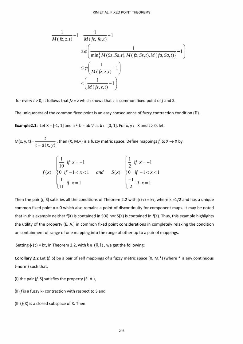
1 11 1( , , ) ( , , )
1 1min ( , , ), ( , , ), ( , , )
1 1( , , )
1 1( , , )
M fz z t M fz fa t
M Sz Sa t M fz Sz t M fa Sa t
M fz z t
M fz z t
for every t > 0, it follows that fz = z which shows that z is common fixed point of f and S.
The uniqueness of the common fixed point is an easy consequence of fuzzy contraction condition (II).
Example2.1: Let X = [-1, 1] and a b = ab a, b [0, 1]. For x, y X and t > 0, let
M(x, y, t) =),( yxdt
t
, then (X, M,) is a fuzzy metric space. Define mappings f, S: X X by
1 11 110 2
( ) 0 1 1 ( ) 0 1 11 11 111 2
if x if x
f x if x and S x if x
if x if x
Then the pair (f, S) satisfies all the conditions of Theorem 2.2 with () = k, where k =1/2 and has a unique
common fixed point x = 0 which also remains a point of discontinuity for component maps. It may be noted
that in this example neither f(X) is contained in S(X) nor S(X) is contained in f(X). Thus, this example highlights
the utility of the property (E. A.) in common fixed point considerations in completely relaxing the condition
on containment of range of one mapping into the range of other up to a pair of mappings.
Setting () = k, in Theorem 2.2, with (0,1)k , we get the following:
Corollary 2.2 Let (f, S) be a pair of self mappings of a fuzzy metric space (X, M,*) (where * is any continuous
t-norm) such that,
(I) the pair (f, S) satisfies the property (E. A.),
(II) f is a fuzzy k- contraction with respect to S and
(III) f(X) is a closed subspace of X. Then
KIM ET AL: FIXED POINT THEOREMS
216

(a) the pair (f, S) has a point of coincidence, whereas
(b) the pair (f, S) has a unique common fixed point provided it is weakly compatible.
Further, if we set
( , , )( , )t
M x y tt d x y
and ),,(),,(),,,(),,,(min tSySxMtSyfyMtSxfxMtSySxM
in Corollary 2.2, then we deduce the following result which is an improvement over a classical result
contained in Jungck [8]. A multitude of such metrical fixed point theorems is available in Imdad and Ali [14].
Corollary 2.3. Let f and S be self mappings of a metric space(X, d) such that,
(I) the pair (f, S) satisfies the property (E. A.),
(II) d (fx, fy) ≤ k d (Sx, Sy), (0,1),k
(III) f(X) is a closed subspace of X.
Then
(a) the pair (f, S) has a point of coincidence, whereas
(b) the pair (f, S) has a unique common fixed point provided it is weakly compatible.
3. Common Fixed Point Theorems via Implicit Functions
We recall the following implicit function was defined and studied by Imdad and Ali [14] and the same was
further utilized to prove some common fixed point theorems. In order to describe this implicit function, let
denote the family of all continuous functions F: [0, 1]4 R satisfying the following conditions:
1F : For every u > 0, v ≥ 0 with F(u, v, u, v) ≥ 0 or F(u, v, v, u) ≥ 0, we have u > v.
2F : F(u, u, 1, 1)< 0, u > 0.
Example 3.1: Define F: [0, 1]4 R as F(t1, t2, t3, t4) = t1 - (min t2, t3, t4). where :[0, 1] [0, 1] is a
continuous function such that (s) > s for 0 < s < 1. Then F.
Example 3.2: Define F(t1, t2, t3, t4): [0, 1]4 R as F(t1, t2, t3, t4)= t1 –k mint2, t3, t4, where k > 1.
Example 3.3: Define F(t1, t2, t3, t4): [0, 1]4 R as F(t1, t2, t3, t4)= t1 –k t2- mint3, t4, where k > 0.
Example 3.4: Define F(t1, t2, t3, t4): [0, 1]4 R as F(t1, t2, t3, t4)= t1 –a t2-bt3-c t4 where a>1 and b, c ≥ 0 (≠1).
KIM ET AL: FIXED POINT THEOREMS
217
Example 3.5: Define F(t1, t2, t3, t4): [0, 1]4 R as F(t1, t2, t3, t4)= t1 –a t2-b(t3+ t4) where a>1 and b ≥ 0 (≠1).
Example 3.6: Define F(t1, t2, t3, t4): [0, 1]4 R as F(t1, t2, t3, t4)= 31t –kt2t3t4 where k > 1.
With a view to generalize some common fixed point theorems contained in Imdad and Ali [12] , we prove
the following fixed point theorem which in turn generalizes several previously known results due to Chugh
and Kumar [3], Vasuki [22] , Turkoglu et al. [20], U. Mishra et al [21] and some others.
Theorem 3.1. Let f, g, S and T be self mapping of a fuzzy metric space(X, M, *). Suppose that
(I) the pair (f, S) (or (g, T)) satisfies the properly (E. A.),
(II) f(X)T(X) (or g(X)S(X)),
(III) S(X) (or T(X)) is a closed subset of X and
(IV) 0)),,(),,,(),,,(),,,(( tTygyMtfxSxMtTySxMtgyfxMF --------------------- (3.1.1)
for all distinct x, y X and t > 0, where F .
Then
(a) the pair (f, S) as well as (g, T) have a point of coincidence each, whereas
(b) f, g, S, and T have a unique common fixed point provided both the pairs (f, S) and (g, T) are weakly
compatible.
Proof. If the pair (f, S) enjoys the property (E.A.), then there exists a sequence nx in X such that
lim lim ,n nn n
fx Sx z
for some zX.
Since f(X) T(X), hence for each xn there exists a yn in X such that n nfx Ty . Therefore,
lim limn nn n
fx Ty z
. Thus, in all we have nfx →z, nSx →z and zTyn . Now, we assert that ngy z .
If not, then using (3.1.1), we have
0)),,(),,,(),,(),,,(( tTygyMtSxfxMtTySxMtgyfxMF nnnnnnnn ,
which on making n→∞, reduces to
(lim ( , , ),1,1, lim ( , , )) 0.n nn n
F M z gy t M gy z t
KIM ET AL: FIXED POINT THEOREMS
218

Implying thereby ),,(lim tgyzM nn
>1, a contradiction. Hence limn
ngy z and in all
lim lim lim lim .n n n nn n n n
fx Sx gy Ty z X
If S(X) is a closed subspace of X, then lim ( )nn
Sx z S X
. Therefore, there exists a point u X such that Su
= z. Now we assert that fu = Su. If not, then using (3.1.1), we have
0)),,(),,,(),,,(),,,(( tTygyMtSufuMtTySuMtgyfuMF nnnn
which on making n reduces to
0)),,(),,,(),,,(),,,(( tzzMtSufuMtzSuMtzfuMF
0)1),,,(,1),,,(( tSufuMtzfuMF
a contradiction to 1F . Hence fu=Su. Therefore, u is a coincidence point of the pair (f, S). Since f(X) T(X) and
( ),fu f X there exists w X such that fu = Tw.
Now, we assert that gw = Tw. If not, then again using (3.1.1), we have
( ( , , ), ( , , ), ( , , ), ( , , )) 0F M fu gw t M Su Tw t M fu Su t M gw Tw t
i.e.
( ( , , ),1,1, ( , , )) 0.F M Tw gw t M gw Tw t
Implying thereby, M(Tw, gw, t)>1, a contradiction. Hence Tw=gw, which shows that w is a coincidence point
of the pair (g, T). Since the pair (f, S) is weakly compatible and fu=Su, hence fz=fSu=Sfu=Sz.
Now, we assert that z is a common fixed point of the pair (f, S). Suppose fz≠z. Then using (3.1.1.),
we have
F(M(fz, gw, t),M(Sz, Tw, t),M(fz, Sz, t),M(gw, Tw, t)) ≥0
or
F(M(fz, z, t),M(fz, z, t),1,1)≥0
which contradict ( 2F ). Hence fz=z. Now, using the notion of the weak compatibility of the pair (g, T) and
inequality (3.1.1), we get gz=z=Tz. Hence z is a common fixed point of both the pairs (f, S) and (g, T).
Uniqueness of z is an easy consequence of contractive condition (3.1.1).
Example 3.7: Let (X, M,) be a fuzzy metric space as defined in the example 2.1 (above) where X = [2, 20].
Now, define mappings f, g, S and T by putting
KIM ET AL: FIXED POINT THEOREMS
219

f2 = 2, fx = 3, if x > 2, S2 = 2, Sx = 6, if x > 2
gx = 2, if x = 2 or x > 5, gx = 5, if 2 < x ≤ 5 and
T2 = 2, Tx = 12, if 2 < x ≤ 5, Tx = (x+1)/3, if x > 5.
We also define F(t1, t2, t3, t4) = t1 - (min t2, t3, t4) with (a) = (7a/3a+4) > a ( , )1
1 d Sx Ty
t
where a
. Then f, g, S
and T satisfy all the conditions of the theorem 3.1 and have a unique common fixed point x = 2.
Here it is worth noting that none of the theorems contained in (Chugh and Kumar [3], Vasuki [22] , Turkoglu
et. al [20], U. Mishra et. al [21], Imdad and Ali [12] ) can be used in the context of this example as Theorem
3.1 never require containment condition in respect of ranges ( g(X) S(X) ) of the involved mappings.
Remark 3.1. The conclusion of theorem 3.1 remains true if for all distinct x,yX, condition (3.1.1) is replaced
by one of the followings conditions:
(I) ( , , ) (min ( , , ), ( , , ), ( , , )),M Ax By t M Sx Ty t M Sx Ax t M By Ty t
where ]1,0[]1,0[: is a continuous function such that )(s > s for all 0 < s < 1.
(II) )),,,(),,,(),,,((min),,( tTyByMtAxSxMtTySxMktByAxM where k > 1.
(III) ),,,(),,,(min),,(),,( tTyByMtAxSxMtTySxkMtByAxM where k > 0.
(IV) ),,,(),,(),,(),,( tTyBycMtAxSxbMtTySxaMtByAxM where a > 1 and )1(0, cb .
(V) )],,,(),,([),,(),,( tTyByMtAxSxMbtTySxaMtByAxM where a > 1 and )1(0 b .
(VI) ),,,(),,(),,(),,( tTyByMtAxSxMtTySxkMtByAxM where k > 1.
Proof: The proof of the corollaries corresponding to contraction conditions (I)-(VI) follows from
Theorem 3.1 and Examples 3.1-3.6.
Remark 3.2: The version of Theorem 3.1 corresponding to condition (I) is a result due to Imdad and
Ali [12] whereas results corresponding to various conditions (II – VI) presents a sharpened form of
Corollary2 of Imdad and Ali [13]. Similarly, from these conditions, we can also deduce generalized
versions of certain results contained in [3, 18, 21, 22].
KIM ET AL: FIXED POINT THEOREMS
220
On the other hand, Singh and Jain [19] also utilized similar implicit function to prove some fixed point
theorems in fuzzy metric spaces. In order to describe such implicit function, let be the set of all real
continuous function : [0, 1]4 R, non decreasing in first argument and satisfying the following conditions:
1 : For u, v ≥ 0, (u, v, u, v) ≥ 0 or (u, v, v, u) ≥ 0 implies that u ≥ v.
2 : (u, u, 1, 1) ≥ 0 implies that u ≥ 1.
Example 3.8: Define (t1, t2, t3, t4) = 15t1 - 13t2 + 5t3 - 7t4. Then, .
Before stating our next result, it may be pointed out that above mentioned two classes of functions and
are independent classes. To substantiate this claim, note that implicit function F(t1, t2, t3, t4)= t1 – k mint2,
t3, t4, where k > 1 (belonging to ) does not belongs to as F (u,u,1,1) < 0 implies u > 0 whereas implicit
function (t1, t2, t3, t4) = 15t1 - 13t2 + 5t3 - 7t4 (belonging to ) does not belongs to as F(u, v, u, v)=0 implies
u=v instead of u > v.
The following theorem is a substantial improvement over Theorem 3.1 contained in Singh and Jain [19].
Theorem 3.2. Let f, g, S and T be self mappings of a fuzzy metric space (X, M, *) which satisfies the
inequalities
( , , ), ( , , ), ( , , ), ( , , ) 0M fx gy kt M Sx Ty t M fx Sx t M gy Ty kt
and
0)),,(),,,(),,,(),,,(( tTygyMktSxfxMtTySxMktgyfxM
for all distinct x, yX and t > 0, (0,1)k where .
Suppose that
(I) the pair (f, S) (or (g, T)) satisfies the properly (E.A.),
(II) f(X)T(X) (or g(X)S(X)),
(III) S(X) (or T(X)) is a closed subset of X and
(a) Then the pairs (f, S) and (g, T) have a point coincidence each, whereas
(b) f, g, S and T have a unique common fixed point provided both the pairs (f, S) and (g, T) are weakly
compatible.
KIM ET AL: FIXED POINT THEOREMS
221
Proof: The proof can be completed on the lines of Theorem 3.1 (above), hence details are omitted.
Corollary 3.1: Let f, g, S and T be four self mappings of a fuzzy metric space (X, M, *) such that pnm Sgf ,,
and qT satisfy the condition (3.1.1). If the pairs ),( pm Sf and ),( qn Tg share the common properly (E.A.)
and ( )pS X as well as )(XT q are a closed subspaces of X, then f, g, S and T have a unique common fixed
point provided the pairs ),( pm Sf and ),( qn Tg commute.
Remark.3.3. Results similar to Corollary 3.1 can be outlined in the context of Theorem 3.2.
Acknowledgement: The authors thank the referee for suggestions to improve upon the original typescript.
References
[1] M. Aamri and D. El Moutawakil: Some new common fixed point theorems under strict contractive
conditions, J. Math. Anal. Appl. 270 (2002), 181-188.
[2] M. Abbas, I. Altun, D. Gopal: Common fixed point theorems for non-compatible mappings in fuzzy metric
spaces, Bull. Math. Anal. Appl., 1(2)(2009), 47-56.
[3] R. Chugh and S. Kumar, Common fixed point theorem in fuzzy metric spaces, Bull. Calcutta Math. Soc.
94(1)(2002), 17-22.
[4] Calogerro-Vetro, Pasquale Vetro: Common fixed points for discontinuous mappings in fuzzy metric
space, Rendiconti del Circolo Matematico di Palermo, 57, (2008), 295-303.
[5] Z. K. Deng: Fuzzy pseudo-metric spaces, J. Math. Anal. Appl. 86, (1982), 74-95.
[6] M.S. El Naschie: On a fuzzy khaler – like manifold which is consistent with two slit experiment, Int. J.
Non-linear Sci. And Numerical Simulation, 6 (2005), 95-98.
[7] A. George and P. Veeramani: On some results of analysis for fuzzy metric spaces, Fuzzy Sets Systems, 90
(1997), 365-368.
[8] G. Jungck: Commuting mappings and fixed points, Amer. Math. Monthly, 83 (1976), 261-263.
[9] G. Jungck: Compatible mappings and common fixed points, Int. J. Math. Math. Sci., 9(4)(1986), 771-779.
[10] O. Kaleva and S. Seikkala: On fuzzy metric spaces, Fuzzy Sets Systems, 27 (1984), 215-229.
[11] O. Kramosil and J. Michalek: Fuzzy metric and statistical metric spaces, Kybernetika, 11 (1975), 326-334.
KIM ET AL: FIXED POINT THEOREMS
222

[12] M. Imdad and Javid Ali: Some common fixed point theorems in fuzzy metric spaces, Math.
Communications, 11(2006), 153-163.
[13] M. Imdad and Javid Ali: Jungck’s Common Fixed Point Theorem and E.A Property, Acta Math. Sinica, English
Series 24(1)(2007), 87-94.
[14] M. Imdad and Javid Ali: A general fixed point theorems in fuzzy metric spaces via implicit function, J.
Appl. Math. And Informatics, 26 (2008), 591-603.
[15] M. Imdad, Javid Ali and M. Tanveer: Coincidence and common fixed point theorems for nonlinear
contractions in Menger PM Spaces, Chaos, Solitons and Fractals, 42(2009), 3121-3129.
[16] P.P. Murthy: Important tools and possible applications of metric fixed point theory, Non-linear Analysis
(T M A) 47 (2001), 3479-3490.
[17] V. Pant: Contractive condition and common fixed points in fuzzy metric spaces, J. Fuzzy Math.
14(2)(2006), 267-272.
[18] B. Singh, M.S. Chauhan: Common fixed point of compatible maps in fuzzy metric spaces, Fuzzy Sets
Systems, 115(2000), 471-475.
[19] B. Singh, S. Jain: Semi compatibility and fixed point theorems in fuzzy metric space using implicit
relation, Int. J. Math. Math. Sci. 16(2005), 2617-2629.
[20] D. Turkoglu, B. E. Rhoades: A fixed fuzzy point for fuzzy mappings in complete metric spaces, Math.
Communications, 10(2)(2005), 115-121.
[21] U. Mishra, A.S. Ranadive, D. Gopal: Some fixed point theorems in fuzzy metric spaces, Tamkang J. of
Math. 30(2009), 419-423.
[22] Vasuki, R.: Common fixed points for R- weakly commuting maps in fuzzy metric spaces, Indian J. Pure
Appl. Math. 39, 4(2008), 309-316.
[23] Zadeh, L.A.: Fuzzy Sets, Inform. & Control, 8(1965), 338-353.
Jong Kyu Kim Department of Mathematics Education Kyungnam University Masan, 631-701, Korea E-mail: [email protected]
KIM ET AL: FIXED POINT THEOREMS
223

M. S. Khan M. Imdad
Department of Mathematics and Statistics Department of Mathematics College of Science, Sultan Qaboos University Aligarh Muslim University, Aligath - 202002 PO Box 36, PCode 123, Al-khod, India Muscat Sultan of Oman Email : [email protected]
Email: [email protected]
D. Gopal
Department of Mathematics and Humanities National Institute of Technology, Surat, Gujarat, India, 395007 Email: [email protected]
KIM ET AL: FIXED POINT THEOREMS
224

Best pSimultaneous Approximaton inLp (;X) :
Eyad Abu-SirhanDepartment of Mathematics,Tala Technical University,
Tala, Jordan
E-mail address: [email protected]
Abstract
Let X be a Banach space and G be a closed subspace of X. Letus denote Lp (;X) ; 1 p < 1; the Banach space of all Xvaluedstrongly measurable functions f on a measure space (;; ) such thatR
kf (s)kp d < 1: In this paper we show that if G is separable and
(;; ) is nte complete measure space, then Lp (;G) is simultane-ously proximinal in Lp (;X) if and only if G is simultaneously proximinalin X:
Math. Subject Classication : 41A28
Keywords : Simultaneous approximation, Banach spaces
1 Introduction
Let X be a Banach space, G a closed subspace of X, and (;; ) be a measurespace.
Denition 1.1 Let (M;d) be a metric space. A Borel measurable functionfrom to M is called strongly measurable if it is the pointwise limit of asequence of simple Borel measurable functions from to M:For 1 p < 1; Lp (;X) is the Banach space consisting of (equivalent
classes of ) strongly measurable functions f : ! X such thatR
kf (s)kp d is
nite, with the usual norm
kfkp =
0@Z
kf (s)kp d
1A 1p
:
1
225
JOURNAL OF APPLIED FUNCTIONAL ANALYSIS, VOL.7, NO. 3,225-235,COPYRIGHT 2012 EUDOXUS PRESS,LLC
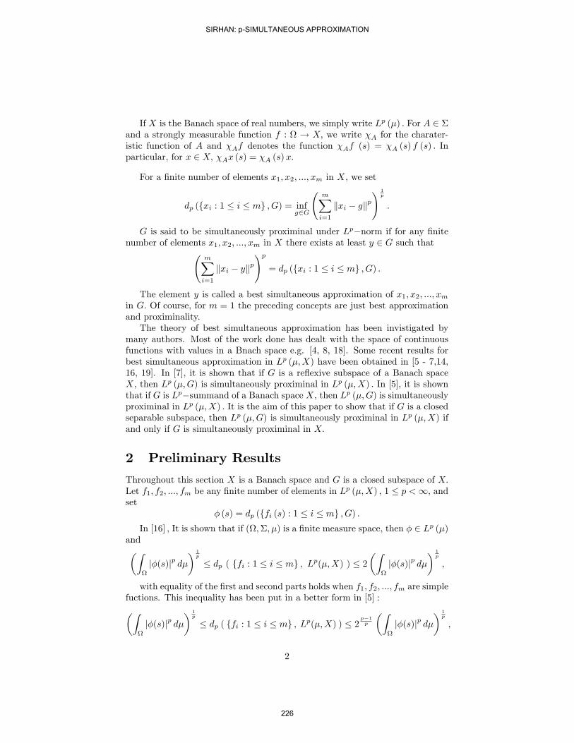
If X is the Banach space of real numbers, we simply write Lp () : For A 2 and a strongly measurable function f : ! X; we write A for the charater-istic function of A and Af denotes the function Af (s) = A (s) f (s) : Inparticular, for x 2 X; Ax (s) = A (s)x:
For a nite number of elements x1; x2; :::; xm in X, we set
dp (fxi : 1 i mg ; G) = infg2G
mXi=1
kxi gkp! 1
p
:
G is said to be simultaneously proximinal under Lpnorm if for any nitenumber of elements x1; x2; :::; xm in X there exists at least y 2 G such that
mXi=1
kxi ykp!p
= dp (fxi : 1 i mg ; G) :
The element y is called a best simultaneous approximation of x1; x2; :::; xmin G: Of course, for m = 1 the preceding concepts are just best approximationand proximinality.The theory of best simultaneous approximation has been invistigated by
many authors. Most of the work done has dealt with the space of continuousfunctions with values in a Bnach space e.g. [4, 8, 18]. Some recent results forbest simultaneous approximation in Lp (;X) have been obtained in [5 - 7,14,16, 19]. In [7], it is shown that if G is a reexive subspace of a Banach spaceX, then Lp (;G) is simultaneously proximinal in Lp (;X) : In [5], it is shownthat if G is Lpsummand of a Banach space X, then Lp (;G) is simultaneouslyproximinal in Lp (;X) : It is the aim of this paper to show that if G is a closedseparable subspace, then Lp (;G) is simultaneously proximinal in Lp (;X) ifand only if G is simultaneously proximinal in X:
2 Preliminary Results
Throughout this section X is a Banach space and G is a closed subspace of X:Let f1; f2; :::; fm be any nite number of elements in Lp (;X) ; 1 p <1; andset
(s) = dp (ffi (s) : 1 i mg ; G) :In [16] ; It is shown that if (;; ) is a nite measure space, then 2 Lp ()
andZ
j(s)jp d 1
p
dp ( ffi : 1 i mg ; Lp(;X) ) 2Z
j(s)jp d 1
p
;
with equality of the rst and second parts holds when f1; f2; :::; fm are simplefuctions. This inequality has been put in a better form in [5] :Z
j(s)jp d 1
p
dp ( ffi : 1 i mg ; Lp(;X) ) 2p1p
Z
j(s)jp d 1
p
;
2
SIRHAN: p-SIMULTANEOUS APPROXIMATION
226
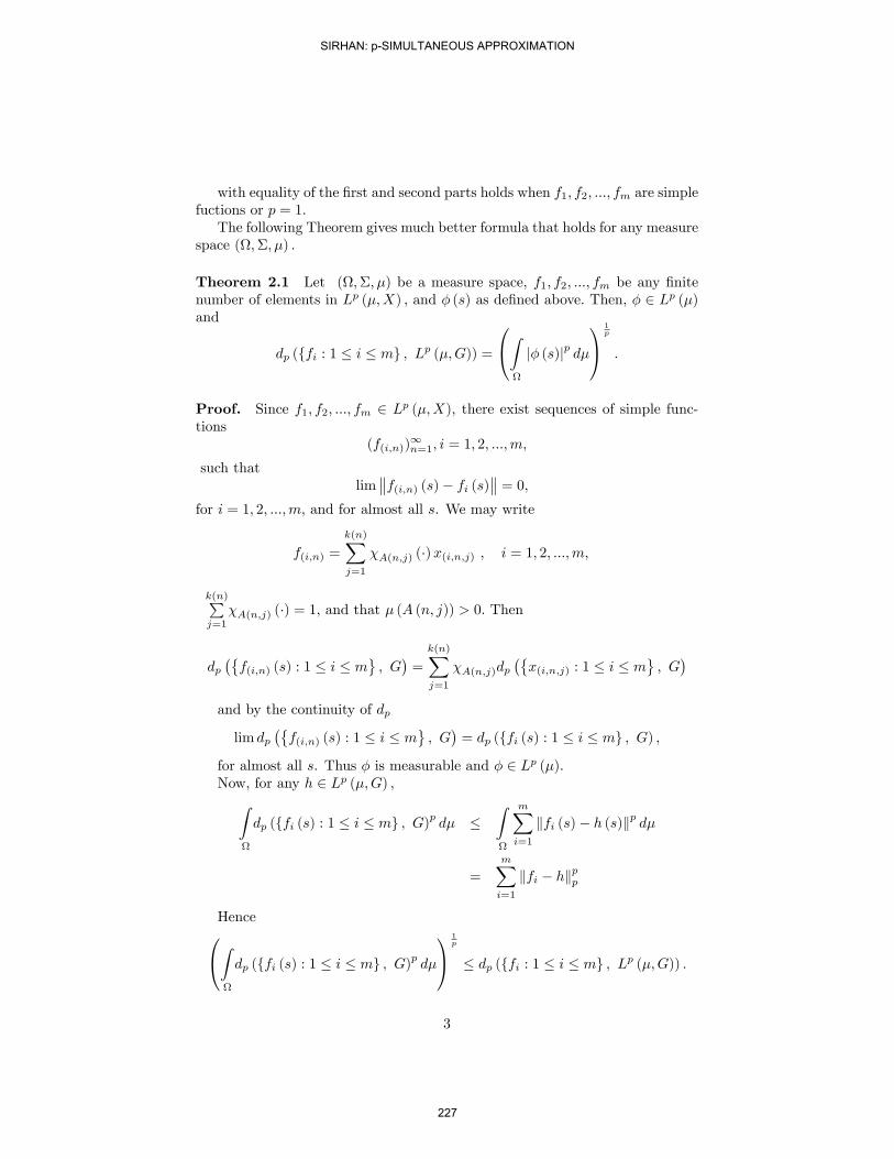
with equality of the rst and second parts holds when f1; f2; :::; fm are simplefuctions or p = 1:The following Theorem gives much better formula that holds for any measure
space (;; ) :
Theorem 2.1 Let (;; ) be a measure space, f1; f2; :::; fm be any nitenumber of elements in Lp (;X) ; and (s) as dened above: Then, 2 Lp ()and
dp (ffi : 1 i mg ; Lp (;G)) =
0@Z
j (s)jp d
1A 1p
:
Proof. Since f1; f2; :::; fm 2 Lp (;X), there exist sequences of simple func-tions
(f(i;n))1n=1; i = 1; 2; :::;m;
such thatlim f(i;n) (s) fi (s) = 0;
for i = 1; 2; :::;m; and for almost all s. We may write
f(i;n) =
k(n)Xj=1
A(n;j) ()x(i;n;j) ; i = 1; 2; :::;m;
k(n)Pj=1
A(n;j) () = 1; and that (A (n; j)) > 0: Then
dpf(i;n) (s) : 1 i m
; G=
k(n)Xj=1
A(n;j)dpx(i;n;j) : 1 i m
; G
and by the continuity of dp
lim dpf(i;n) (s) : 1 i m
; G= dp (ffi (s) : 1 i mg ; G) ;
for almost all s. Thus is measurable and 2 Lp ().Now, for any h 2 Lp (;G) ;Z
dp (ffi (s) : 1 i mg ; G)p d Z
mXi=1
kfi (s) h (s)kp d
=mXi=1
kfi hkpp
Hence0@Z
dp (ffi (s) : 1 i mg ; G)p d
1A 1p
dp (ffi : 1 i mg ; Lp (;G)) :
3
SIRHAN: p-SIMULTANEOUS APPROXIMATION
227

To prove the reverse inequality, let > 0 be given and wi; i = 1; 2; :::;m; besimple functions in Lp (;X) such that
kfi wikp <
3m1p
:
We may write wi =P`
k=1 Ak() x(i;k);
Pk=1
Ak() = 1; and that (Ak) > 0:
Since wi 2 Lp (;X) for all i; we have x(i;k) (Ak) < 1 for all k and i: If
(Ak) <1; select hk 2 G so thatmXi=1
x(i;k) hk p < dp x(i;k) : 1 i m ; Gp + p
3p (Ak);
for all k: If (Ak) =1; put hk = 0:Let g =
P`k=1 Ak
()hk: It is clear that g 2 Lp (;G) : Then
dp (ffi : 1 i mg ; Lp (;G))
mXi=1
kfi gkpp
! 1p
=
mXi=1
kfi wi + wi gkpp
! 1p
mXi=1
kfi wikpp
! 1p
+
mXi=1
kwi gkpp
! 1p
<
mXi=1
p
3pm
! 1p
+
mXi=1
kwi gkpp
! 1p
=
3+
mXi=1
Xk=1
(Ak) x(i;k) hk p
! 1p
=
3+
Xk=1
mXi=1
(Ak) x(i;k) hk p
! 1p
=
3+
Xk=1
(Ak)mXi=1
x(i;k) hk p! 1
p
3+
Xk=1
(Ak) dpx(i;k) : 1 i m
; Gp+p
3p
! 1p
4
SIRHAN: p-SIMULTANEOUS APPROXIMATION
228

3+
Xk=1
(Ak) dpx(i;k) : 1 i m
; Gp! 1
p
+
p
3p
1p
=2
3+
0@Z
Xk=1
Ak(s) dp
x(i;k) : 1 i m
; Gpd
1A 1p
=2
3+
0@Z
dp (fwi (s) : 1 i mg ; G)p d
1A 1p
2
3+
0@Z
24dp (ffi (s) : 1 i mg ; G) + mXi=1
kfi (s) wi (s)kp! 1
p
35p d1A
1p
Using triangle inequality in Lp () so that the right hand side becomes
2
3+
26664R
dp (ffi (s) : 1 i mg ; G)p d 1
p
+
R
Pmi=1 kfi (s) wi (s)k
pd
1p
37775
2
3+
0@Z
dp (ffi (s) : 1 i mg ; G)p d
1A 1p
+
mXi=1
kfi wikpp
! 1p
2
3+
0@Z
dp (ffi (s) : 1 i mg ; G)p d
1A 1p
+
3
+
0@Z
dp (ffi (s) : 1 i mg ; G)p d
1A 1p
:
This ends the proof.
Corollary 2.2 Let (;; ) be a measure space, f1; f2; :::; fm be any nitenumber of elements in Lp (;X) : Let g : ! G be a measurable functionsuch that g (s) is a best simultaneous approximation of f1 (s) ; f2 (s) ; :::; fn (s)for almost all s: Then g is a best simultaneous approximation of f1; f2; :::; fn inLp (;G) ( and therefore g 2 Lp (;G)):
5
SIRHAN: p-SIMULTANEOUS APPROXIMATION
229
Proof. Assume that g (s) is a best simultaneous approximation of f1 (s) ; f2 (s) ; :::; fm (s)for almost all s:Then
mXi=1
kfi (t) g (t)kp! 1
p
mXi=1
kfi (t) zkp! 1
p
;
for almost all s, and for all z 2 G: Then, set z = 0 and use triangle inequalityof Lpnorm,
mXi=1
kg (t)kp! 1
p
2
mXi=1
kfi (t)kp! 1
p
;
for almost all s; therefore g 2 Lp (;G) : By Theorem 2.1,
dp (ffi : 1 i mg ; Lp (;G))p =
Z
dp (ffi (s) : 1 i mg ; G)p d
=
Z
mXi=1
kfi (s) g (s)kp d
=
mXi=1
kfi gkpp :
Therefore g is a best simultaneous approximation for f1; f2; ::; fm in Lp (;G) :
The condition in Corollary 2.2 is su¢ cient ; g (s) is a best simultaneousapproximation of f1 (s) ; f2 (s) ; :::; fm (s) for almost all s in G; implies g is abest simultaneous approximation of f1; f2; :::; fm in Lp (;G) : In fact we havethe following theorem :
Theorem 2.3. Let (;; ) be a measure space. Then, Lp (;G) is simulta-neously proximinal in Lp (;X) if and only if for any nite number of elementsf1; f2; :::; fm in Lp (;X) ; there exists g 2 Lp (;G) such that g (s) is a bestsimultaneous approximation of f1 (s) ; f2 (s) ; :::; fn (s) for almost all s:
Proof. Su¢ ciency of the condition is an immediate consequence of Corollary2.2. We will show the necessity. Assume that Lp (;G) is simultaneously prox-iminal in Lp (;X) and let f1; f2; :::; fm be any nte number of elements inLp (;X) : Then, there exists g 2 Lp (;G) such that
mXi=1
kfi gkpp = dp (ffi : 1 i mg ; Lp (;G))p
=
Z
dp (ffi (s) : 1 i mg ; G)p d;
6
SIRHAN: p-SIMULTANEOUS APPROXIMATION
230
henceZ
mXi=1
kfi (s) g (s)kp dp (ffi (s) : 1 i mg ; G)p!d = 0:
ThusmXi=1
kfi (s) g (s)kp = dp (ffi (s) : 1 i mg ; G)p ;
for allmost all s:
3 Main Result.
Let (;; ) be a measure space and X be a Banach space: We say that f : ! X is measurable in the classical sense if f1 (O) is measurable for everyopen set O X:The following lemmas will be used to prove our main result.
Lemma 3.1 [21] . Let (;; ) be a complete measure space and X be aBanach space. If f is a strongly measurable functon from to X; then f ismeasurable in the classical sense.
Lemma 3.2 [21] . Let (;; ) be a complete measure space and X be aBanach space. If f : ! X is measurable in the classical sense and hasessetially seprable range, then f is srongly measurable.
Let be a set-valued mapping, taking each piont of a measurable space into a subset of a metric space X:We say that is weakly measurable if 1(O)is measurable in whenever O is open in X: Here we have put, for any A X;
1(A) = fs 2 : (s) \A 6= g:
The following theorem is due to Kuratowski [15], it is known as MeasurableSelection Theorem.
Theorem 3.3 [15] . Let be a weakly measurable set-valued map whichcarries each piont of a measurable space to a closed nonvoid subset of acomplete seprable metric space X. Then has a measurable selection; i.e.,there exists a function f : ! X such that f(s) 2 (s) for each s andf1(O) is measurable in whenever O is open in X:
7
SIRHAN: p-SIMULTANEOUS APPROXIMATION
231
Theorem 3.4. Let X be a Banach space and G be a closed seprable subspaceof X; and (;; ) is nite complete measure space. Then the following areequivalent :
1. G is simultaneously proximinal in X:
2. Lp (;G) is simultaneously proximinal in Lp (;X) :
Proof. (2) ) (1) : Let x1; x2; :::; xm be any nite number of elements in X:Since (;; ) is nite, we can assume that = [
n2NAn such that (An) <
1 for all n 2 N: Then there must be k0 2 N such that 0 < (Ak0) <1: Denefxi : ! X; i = 1; 2; :::;m; by
fxi (s) = (Ak0)1p1 Ak0
(s)xi;
for all s 2 : Then fxi 2 Lp (;X) for all i: By the assumption, there existsf0 2 Lp (;G) such that
mXi=1
kfxi f0kpp
!1=p= dp (ffxi : 1 i mg ; Lp (;G)) :
Then mXi=1
kfxi f0kpp
!1=p
mXi=1
fxi (Ak0) 1p1 Ak0g pp
!1=p
= (Ak0)1p1
mXi=1
Ak0xi Ak0
g pp
!1=p
= (Ak0)1p1
0B@ZAk0
mXi=1
kxi gkp!d
1CA1=p
= (Ak0)2p1
mXi=1
kxi gkp!1=p
;
for all g 2 G: By Theorem 2.3 , f0 (s) is a best simultaneous approximationof fx1 (s) ; fx2 (s) ; :::; fxm (s) for almost all s: Then
mXi=1
kfxi (s) f0 (s)kp
!1=p
mXi=1
kfxi (s) h (s)kp
!1=p;
for almost all s and for any strongly measurable function h : ! G; hence
8
SIRHAN: p-SIMULTANEOUS APPROXIMATION
232

f0 = Ak0f0: Put x0 =
RAk0
f0 (s) d: Then
mXi=1
xi x0
(Ak0)1p
p!1=p
= (Ak0) 1p
0B@ mXi=1
ZAk0
fxi (s) dZAk0
f0 (s) d
p1CA
1=p
(Ak0) 1p
0B@ mXi=1
0B@ZAk0
kfxi (s) f0 (s)k d
1CAp1CA
1=p
(Ak0) 1p
2664 mXi=1
0BB@0B@Z
Ak0
kfxi (s) f0 (s)kpd
1CA1=p
( (Ak0))11=p
1CCAp3775
1=p
= (Ak0)1 2
p
mXi=1
kfxi f0kpp d
!1=p
mXi=1
kxi gkp!1=p
;
for all g 2 G: Hence 1
(Ak0)1px0 is a best simultaneous approximation of
x1; x2; :::; xm in G:(1) ) (2) : Let f1; f2; :::; fm be any nite number of elements in Lp (;X) :
For each s 2 dene
(s) =
8<:g 2 G :
mXi=1
kfi (s) gkp!1=p
= dp (ffi (s) : 1 i mg ; G)
9=; :For each s 2 ; (s) is closed, bounded, and nonvoid subset of G: We shall
show that is weakly measurable. Let O be an open set in X; the set
1(O) = fs 2 : (s) \O 6= g
can be also be described as
1(O) = fs 2 : infg2G
mXi=1
kfi (s) gkp!1=p
= infg2O
mXi=1
kfi (s) gkp!1=p
g:
Since (;; ) is complete, fi is measurable in the classical sence for i =1; 2; :::;m by Lemma 3.1. Since subtraction in G; sum; and the norm in X arecontinuous, then the map
s! infg2A
mXi=1
kfi (s) gkp!1=p
9
SIRHAN: p-SIMULTANEOUS APPROXIMATION
233

is measurable for any set A: It follows that 1(O) is measurable. ByTheorem 3.3, has a measurable selection; i.e., there exists a function f :! G such that f(s) 2 (s) for each s and f is measurable in the classicalsense. By Lemma 3.2, f is strongly measurable. Hence f is a best simultaneousapproximation for f1; f2; :::; fm in Lp (;G) by Corollary 2.2.
References
[1] A.P. Bosznoy, A remark on simultaneous approximation , J. Approx. The-ory 28 (1978), 296-298.
[2] A.S. Holland, B.N. Sahney, and J.Tzimbalario, On best Simultaneous Ap-proximation , J. Indian Math. Soc. 40 (1976),69-73.
[3] C. B. Dunham, Simultaneous Chebyshev Approximation of Functions onan Interval, Proc. Amer. Math. Soc.18 (1967), 472-477.
[4] Chong Li, On Best Simultaneous Approximation, J. Approx. Theory 91,(1998) 332-348.
[5] E. Abu-Sirhan, Best simultaneous approximation in Lp (I;X) ; Inter. J.Math. Analysis, vol. 3, no. 24, (2009) 1157-1168.
[6] E. Abu-Sirhan and R. Khalil, Best Simultaneous Approximation in Func-tion Spaces, Inter. J. Math. Analysis, vol. 2, no. 5, (2008) 207-212.
[7] Fathi B. Saidi, Deep Hussein, and R. Khalil, Best Simultaneous Approxi-mation in Lp(I; E), J. Approx. Theory 116 (2002), 369-379.
[8] G. A. Watson, A Charaterization of Best Simultaneous approximation, J.Approx. Theory 75, (1998) 175-182.
[9] JarosLav Mach, Best Simultaneous Approximation of Bounded Functionswith Values in Certain Banach Spaces, Math. Ann. 240, 157-164 (1979).
[10] J. Diestel and J.R. Uhl, Vector Measures, Math. Serveys Monograghs.Vol.15, Amer. Math. Soc., Providence, RI, 1977.
[11] J.B. Diaz and H.W. McLaughlin, On simultaneous Chebyshev Approxi-mation and Chebyshev Approximation with an additive weight function,J.Approx. Theory 6 (1972),68-71.
[12] J.B. Diaz and H.W. McLaughlin, Simultaneous Approximation of a Set ofBounded Real Functions, Math. Comp. 23 (1969),583-593.
[13] J. Mendoza, Proximinality in Lp (;X) ; J. Approx. Theory 93, 331-343(1998).
10
SIRHAN: p-SIMULTANEOUS APPROXIMATION
234

[14] J. Mendoza and Tijani Pakhrou, Best Simultaneous Approximation inL1 (;X) , J. Approx. Theory 145, (2007) 212-220.
[15] K. Kuratowiski and C. Ryll-Nardzewski, A General Theorem on Selectors,Bull. Acad. Polonaise Sciences, Serie des Sciences Math. Astr. Phys. 13(1965), 379-403 MR 32. #6421.
[16] M. Khandaqji and W. Shatanawi,Best pSimultaneous Approximation insome Metric Space, Turk. J. Math. 32 (2008) ; 1 9
[17] Mun Bae Lee and Sung Ho Park, Proximity Maps for Certain Spaces,Korean Math. Soc. 34 No. 2 (1997) ; 259-271.
[18] Shinji Tanimoto, On Simultaneous Approximation, Math. Japanica 48, No.2 (2007) 275-279.
[19] Tijani Pakhrou, Best Simultaneous Approximation in L1 (;X) ; Math.Nacher. 281, No. 3, (2008) 396-401:
[20] W.A Light, Proximinality in Lp(I;X),J. Approx. Theory 19 (1989), 251-259.
[21] W.A Light and E.W. Cheney, Approximation Theory in Tensor ProductSpaces, Lecture Notes in Mathematics,1169, Spinger-Verlag, Berlin Heidel-berg New York Tokyo(1985).
11
SIRHAN: p-SIMULTANEOUS APPROXIMATION
235
WHEN AN EXPOSED POINT OF A CONVEX SET IS AREMOTAL POINT
KHALIL, R. 1 AND AL-HAWAWSHA, L.2
Abstract. Let X be a Banach space and Y be a closed bounded subset ofX: We call Y remotal in X if for every x 2 X there exists some y 2 Y suchthat kx yk kx zk 8z 2 Y: It is called uniquely remotal in X if forevery x 2 X there is a unique y 2 Y such that kx yk kx zk 8z 2 Y: Inthis paper we study the remotality of exposed points of convex sets in Banachspaces.
1. Introduction
Let X be a Banach space and E be a closed bounded set of X: For x 2 X, let
D(x;E) = supe2E
kx ek :
This supremum need not be attained. If 8x 2 X; there exists some e 2 E suchthat D(x;E) = kx ek ; then E is called remotal. Forx 2 X, we set
F (x;E) = fe 2 E : kx ek = D(x;E)gThe point e is called a farthest point of E from x: The study of remotal
sets goes back to the sixties. Edelstein (1966) showed that if X is a uniformlyconvex Banach space, then the set of points in X that has farthest points in Eare dense in X: The importance of the study of remotal sets comes from its ties togeometry of Banach spaces. Such study is little di¢ cult and less developed. Onthe contrary, closest points are well studied and well established. The problem ofremotality in Lp(I;X) 1 p <1; was initiated by Khalil and Al-Sharif [2]. Thenit was developed by Sababhah and Khalil [5]. One of the standing conjecturesin the theory of remotal sets is "Every uniquely remotal set in a Banach spaceis a singleton". So much work was done to solve such a conjecture, We referto Astaneh [1], Narang [3], and Sababhah and Khalil [6,7] and , for more andreferences on such a problem.Another problem in the theory of remotal sets is" When is a boundary point
of a set a farthest point from some point in X?" It is the object of this paper tostudy such a problem.
2000 Mathematics Subject Classication. 41A65, 41A28.Key words and phrases. Remotal sets, Approximation theory in Banach spaces.
1
236
JOURNAL OF APPLIED FUNCTIONAL ANALYSIS, VOL.7, NO. 3,236-240,COPYRIGHT 2012 EUDOXUS PRESS,LLC

2 KHALIL, R. AND AL-HAWAWSHA, L.
2. Remotality Of Exposed Points
In this section we introduce new results that partially answer the followingprimary question " when an exposed point must be a farthest point from somepoint in X ?".
Lemma 2.1 : There exist convex sets with extreme points that are not remotalpoints.Proof :
Let X = R2. Let S1 be the unit circle in X when endowed with the Euclidiannorm and let S2 be the unit circle in X when endowed with the sup norm. Let Ebe the convex hull of the union of f(x; y) 2 S1 : x 0g and f(x; y) 2 S2 : x 0g.It is clear that the point A(0; 1) is an extreme point of E. We assert that A isnot a remotal point. That is, we show that A =2 F (x;E) for any x 2 X, X beingendowed with the Euclidian norm. To do so, we use Lemma 2.1. Thus, supposeon the way of contrary that a circle x2 + y2 + ax + by + c = 0 exists such thatA belongs to the circle and such that E is inside the circle. For A to be on thecircle, we need to have c = b 1. Hence, the equation of the circle becomesx2+ y2+ ax+ by = b+1. Since E lies inside the circle, B(1; 1); C(1;1) andD(1; 0) must be inside the circle. Now, for Bto be inside the circle we must havea 1 and for D to be inside the circle we need to have a b. Now let (x; y)be any point on the right half of the unit circle. That is x2 + y2 = 1 and x 0.The question is Does (x; y) lie inside the circle x2 + y2 + ax + by = b + 1?Thatis Does (x; y) satisfy x2 + y2 + ax + by b + 1?. Since x2 + y2 = 1, we need tocheck whether ax + by b or not. Thus the question reduces to: What is themaximum value of ax+ by subject to the conditions x2+ y2 = 1and x 0? If weuse the method of Lagrange multipliers we nd that the point( ap
a2+b2, bpa2+b2
) is on the right half of the unit circle which lies outside thecircle x2 + y2 + ax+ by = b+ 1.This shows that no circle passing through A cansatisfy the conditions of Lemma 2.1. Hence, A is not a remotal point of E.
Denition 2.2 : an exposed point e of a convex set E is a boundary point ofE such that a functionalf 2 X exists with the properties f(e) = and f(x) < 8x 2 Enfeg.In other words, it means that a hyperplane H exists such that e is the only
element of E that belongs to H , and E lies entirely on one side of H.
Lemma 2.3 : There are closed bounded convex sets in Hilbert spaces whoseexposed points are not necessarily remotal points.
Proof : Let X be R2 endowed with Euclidean norm and letE0 = f( 1
n; 1n3) : n 2 Ng
If E is the closed convex hull of E0, then clearly E lies above the x-axis whichtouches E uniquely at (0; 0). That is, (0; 0) is an exposed point of E. We assertthat (0; 0) is not a remotal point for E. Observe that if (x; y) 2 X then
237
UNIQUELY REMOTAL SETS 3
k (x; y) ( 1n; 1n3) k2= (x2 + y2) + ( 1
n2+ 1
n6) + ( 2
nx 2
n3y)
= (x2 + y2) + ( 1n6 2
nx) + ( 1
n2 2
n3y):
Observe that n 2 N can be chosen so that ( 1n2 2
n3y) > 0 for a given y: As for
( 1n6 2
nx);one can manage to have the plus or the minus n, according to whether
x is negative or positive, in order to make ( 1n6 2
nx) > 0: These observations
together tell us that
k (x; y) ( 1n; 1n3) k2> x2 + y2 =k (x; y) (0; 0) k :
That is, (0; 0) cannot be a farthest point in E from (x; y). In other words,(0; 0) is not a remotal point of E.
Denition 2.4 Let X be a normed space and E be a bounded closed subsetof X. For e 2 @E(in spanE), we dene C(E; e) = f(x e) : > 0; x 2 Xg:This is called the cone generated by with E vertex e.
Example 2.5: Let E = f(x; y) : 0 x 1; 0 y 1g. Then C(E; (0; 0)) isthe rst quadrant.
Example 2.6: Let E = f(x; y) : x2 + y2 = 1g: Then C(E; (0; 0)) = R2:
Remark 2.7.We should remark that any two dimensional normed space Xhave an equivalent norm that makes it isometricallyisomorphic to R2 with the Euclidean norm. The angle between two rays in X,
is the angle between them when X is mapped ontoR2 isometrically.
Denition 2.8. Let X be a normed space and E be a bounded closed subsetof X. If e is an exposed point of E dene
(C(E; e); H) = inf f(x; y) : x 2 H , y 2 C(E; e)gwhere H is the hyper plane exists by e, and (x; y) is the angle between the
two segment [e; x;] and [e; y;] as in Remark 4.3.:
Denition 2.9: Let E be a closed convex bounded set of a Banach space X,and e be an exposed point of E. The point e is called cone remotal if and onlyif there is a subset B of E and x in E such that D(x;E) = D(x;B = kx ekand (C(B; e); H) > 0:
Remark 2.10: It is obvious from denition that if e is a cone remotal pointthen e is a remotal point.Theorem 2.11: Let E be a closed bounded convex set of a Banach space X.
Assume that e is a remotal exposed point of E. Then e is cone remotal.Proof:Assume that e is a remotal exposed point of E. Thus there exits x in X
such that D(x;E) = kx ek : Consider [x; e] \ E: Then B = [z; e] E: Now,
238

4 KHALIL, R. AND AL-HAWAWSHA, L.
any hyper plane supporting E at e has a positive angle with [z; e]. Hence(C(B; e); H) > 0:Since D(x;E) = D(x;B) = kx ek ; then e is cone remo-tal. This completes the proof.
Lemma 2.12: Let X be a reexive Banach space, and H = fz : f(z) = 0gfor some f 2 X: Then there exits an x 2 X such that kxk = d(x;H):Proof. Let z be any element inX: SinceX is reexive, thenH is proximinal.
Hence there exists y 2 H such that kz yk kz hk for all h 2 H: Now, letx = z y: Since H is a subspace, then y + w 2 H for all w 2 H: hencekxk = kz yk kz (y + w)k = kx wk for all w 2 H: Hence kxk = d(x;H):
Lemma 2.13 : Let X be any normed space, and T : X ! X be dened byT (x) = x + a for some xed a in X: Then T preserves extreme and exposedpoints of convex sets of X:Proof. We prove the case of extreme points. So, let E be a closed convex set
in a normed space X; and e be an extreme point of E:We claim that e+ a is an extreme point of E + a = fx+ a : x 2 Eg: Indeed,
if possible, assume e+ a is not an extreme point of E + a: Thene+ a = 1
2[(x+ a) + (y + a)] for some x; y 2 E: But that implies e = 1
2(x+ y);
and e is not an extreme point.
Theorem 2.14. Let X be a uniformly convex Banach space, and E bea closed bounded convex set of X: If e is an exposed point of E such that(C(E; e); H) > 0; for some hyperplane supporting E at e, then e is a remotalpoint of E:Proof. Since e is an exposed point of E; there is at least one hyperplane H
that supports E at e only. That is H \ E = feg: However, since X is reexive,one can use Lemma 4.1, and Lemma 4.2 to assume without any loss of generalitythat e = 0:Again, since X is reexive, then H is proximinal. Further, being a subspace,
then for every point z 2 H; there exists a point x 2 Xsuch that kx zk = d(x;H): Thus, there is some x 2 H such that kxk =
d(x;H): Further, we can choose the x on the same side of the set ENow, kxk kx zk for all z 2 H: But this implies that ktxk ktx zk for
all z 2 H and all t > 0: Indeed ktxk = t kxk t kx zk = ktx tzk for allz 2 HSince H is a subspace, then tz 2 H: Further, and w 2 H is of the form
w = twt= tz for some z 2 H: Hence ktxk ktx zk for all z 2 H: Now
consider, B[tx; ktxk]: These balls touches the hyperplane H at 0 for all t > 0:Now, if for some t > 0; E B[tx; ktxk]; then E is remotal.If possible assume that there is no t > 0; such that E B[tx; ktxk]: This
implies there is a sequence tn such that for each n; there issome en 2 E and ktnx enk > ktnxk : Further, since X is uniformly convex,
d(en; H)! 0; for otherwise, some ball B[tx; ktxk] (for some t; will contain all ofthe e;sn ): But in this case, (C(E; e); H) = 0:This contradicts the assumption. Hence E is remotal.
239

UNIQUELY REMOTAL SETS 5
We end this paper with the following questionsQuestion1. Can one give a necessary and su¢ cient conditions for an exposed
point in reexive spaces to be remotal?Question 2. Can one prove Theorem 2.14 in general Banach spaces?Question 3. When a boundary point in a closed convex bounded set in a Banach
space is a remotal point?Question 4. Can one improve Theorem 2.14?
REFERENCES[1] Astaneh, A., On Uniquely Remotal Subsets of Hilbert spaces, Indian Jour-
nal Of Pure and Applied Mathematics. 14(10)(1983), pp. 1311-1317.
[2] Khalil, R. and Al-Sharif, Sh., Remotal sets in vector valued function spaces,Scientiae Mathematicae Japonica, 63(2007), no. 3, pp.433-441.
[3] Narang, T.D., On singletoness of uniquely remotal sets, Periodica Math-ematika Hungarica. 21(1990), pp. 17-19.
[4] Narang, T. D. A study of farthest points, Nieuw Arch. Wish. 2(1977)54-79.[5] Sababheh, M. and Khalil, R.Remarks on remotal sets in vector valued func-
tion spaces.The Journal of Nonlinear Sciences and Applications Vol. 2No. 1, (2009) pp. 1-10.[6] Sababheh, M. and Khalil, R. New results on remotality of sets in Banach
spaces. Italian J. of Pure and Applied Mathematics. To appear.
[7] Sababheh, M., Khalil, R., Remotality of closed bounded convex sets in re-exive spaces, Numerical Functional analysis and optimization, 29 (2008),pp.1166-1170.
1 Department of Mathematics, Jordan University, Al Jubaiha, Amman 11942,Jordan.E-mail address: [email protected]
240
DOUBLE MULTIPLIER SEQUENCE SPACES OF FUZZY NUMBERS
DEFINED BY A SEQUENCE OF ORLICZ FUNCTION
KULDIP RAJ, AJAY K. SHARMA, ANIL KUMAR AND SUNIL K. SHARMA
Abstract. In this paper we introduce some double sequence spaces of Fuzzy numbers
defined by a sequence of Orlicz function M = (Mkl) and a multiplier function u =(ukl). We also make an efforts to prove some topological properties and inclusion
relations between these spaces.
1. Introduction
Fuzzy set theory, compared to other mathematical theories, is perhaps the most easilyadaptable theory to practice. The main reason is that a Fuzzy set has the property ofrelativity, variability and inexactness in the definition of its elements. Instead of definingan entity in calculus by assuming that its role is exactly known, we can use Fuzzy setsto define the same entity by allowing possible deviations and inexactness in its role. Thisrepresentation suits well the uncertainties encountered in practical life, which make Fuzzysets a valuable mathematical tool. The concepts of Fuzzy sets and Fuzzy set operationswere first introduced by Zadeh [7] and subsequently several authors have discussed vari-ous aspects of the theory and applications of Fuzzy sets such as Fuzzy topological spaces,similarity relations and Fuzzy orderings, Fuzzy measures of Fuzzy events, Fuzzy mathe-matical programming. Matloka [9] introduced bounded and convergent sequences of Fuzzynumbers and studied some of their properties.In particular the concept of Fuzzy topology has very important applications in quantumparticle physics, especially in the connections with both string and ε∞ theory which weregiven and studied by El Naschie [8]. In [12], Nanda studied on sequences of Fuzzy numbersand showed that the set of all convergent sequences of Fuzzy numbers forms a completemetric space.The idea of statistical convergence of a sequence was introduced by Fast [5]. Statisticalconvergence was generalized by Buck [11] and studied by other authors, using a regularnonnegative summability matrix A in place of Cesaro matrix. The existing literature onstatistical convergence appears to have been restricted to real or complex analysis, butat the first time Nurray and Savas [4] extended the idea to apply the sequences of Fuzzynumbers. For more details on Fuzzy sequence spaces see ([2], [3]) and references therein.
2. Definitions and preliminaries
An Orlicz function is a functionM : [0,∞)→ [0,∞) which is continuous, non decreasingand convex with M(0) = 0, M(x) > 0 for x > 0 and M(x)→∞ as x→∞.Lindenstrauss and Tzafriri [6] used the idea of Orlicz function to define the following
2000 Mathematics Subject Classification. Primary 40H05; Secondary 40C05.Key words and phrases. Fuzzy numbers, Orlicz function, de La Vallee-Poussin means, statistical con-
vergence, multiplier function.
1
241
JOURNAL OF APPLIED FUNCTIONAL ANALYSIS, VOL.7, NO. 3,241-247,COPYRIGHT 2012 EUDOXUS PRESS,LLC

2 KULDIP RAJ, AJAY K. SHARMA, ANIL KUMAR AND SUNIL K. SHARMA
sequence space. Let w be the space of all real or complex sequences x = (xk), then
lM =x ∈ w :
∞∑k=1
M( |xk|ρ
)<∞
which is called as an Orlicz sequence space. Also lM is a Banach space with the norm
‖x‖ = infρ > 0 :
∞∑k=1
M( |xk|ρ
)≤ 1.
Also, it was shown in [6] that every Orlicz sequence space lM contains a subspace iso-morphic to lp(p ≥ 1). The ∆2-condition is equivalent to M(Lx) ≤ LM(x), for all L with0 < L < 1. An Orlicz function M can always be represented in the following integral form
M(x) =
∫ x
0
η(t)dt
where η is known as the kernel of M , is right differentiable for t ≥ 0, η(0) = 0, η(t) > 0, ηis non-decreasing and η(t)→∞ as t→∞.A Fuzzy number is a Fuzzy set on the real axis, i.e., a mapping X : Rn → [0, 1] whichsatisfies the following four conditions :
(1) X is normal, i.e., there exist an x0 ∈ Rn such that X(x0) = 1;(2) X is Fuzzy convex, i.e., for x, y ∈ Rn and 0 ≤ λ ≤ 1, X(λx + (1 − λ)y) ≥
min[X(x), X(y)];(3) X is upper semi-continuous;(4) the closure of x ∈ Rn : X(x) > 0, denoted by [X]0, is compact.
The set of all upper-semi continuous, normal, convex Fuzzy real numbers is denoted byR(I).
Let C(Rn) = A ⊂ Rn : A compact and convex . The spaces C(Rn) has a linearstructure induced by the operations
A+B = a+ b, a ∈ A, b ∈ B
and
λA = λa, λ ∈ Afor A,B ∈ C(Rn) and λ ∈ R. The Hausdorff distance between A and B of C(Rn) is definedas
δ∞(A,B) = maxsupa∈A
infb∈B‖a− b‖, sup
b∈Binfa∈A‖a− b‖
where ‖.‖ denotes the usual Euclidean norm in Rn. It is well known that (C(Rn), δ∞) is acomplete (not separable) metric space.For 0 < α ≤ 1, the α-level set
Xα = x ∈ Rn : X(x) ≥ α
is a nonempty compact convex, subset of Rn, as is the support X0. Let L(Rn) denote theset of all Fuzzy numbers. The linear structure of L(Rn) induces addition X+Y and scalarmultiplication λX, λ ∈ R, in terms of α-level sets, by
[X + Y ]α = [X]α + [Y ]α
and
[λX]α = λ[X]α
FUZZY NUMBERS...ORLICZ FUNCTION
242
3
for each 0 ≤ α ≤ 1. Define for each 1 ≤ q <∞
dq(X,Y ) =∫ 1
0
δ∞(Xα, Y α)qdα 1
q
and d∞(X,Y ) = sup0≤α≤1
δ∞(Xα, Y α). Clearly d∞(X,Y ) = limq→∞
dq(X,Y ) with dq ≤ dr if
q ≤ r. Moreover dq is a complete, separable and locally compact metric space [10].In this paper, d will denote dq with 1 ≤ q ≤ ∞.
A Fuzzy double sequence is a double infinite array of Fuzzy numbers. We denote a Fuzzydouble sequence by (Xmn), where Xmn’s are Fuzzy numbers for each m,n ∈ N. By s′′(F )we denote the set of all double sequences of Fuzzy numbers.
Definition ([1]) A double sequence X = (Xkl) of Fuzzy numbers is said to be convergentin the Pringsheim’s sense or P -convergent to a Fuzzy number X0, if for every ε > 0 thereexists N ∈ N such that
d(Xkl, X0) < ε for k, l > N,
where N is the set of natural numbers, and we denote by P − limX = X0. The numberX0 is called the Pringsheim limit of Xkl.More exactly we say that a double sequence (Xkl) converges to a finite number X0 if Xkl
tend to X0 as both k and l tends to ∞ independently of one another.
Let M = (Mkl) be a sequence of Orlicz function, p = (pkl) be a factorable double se-quence of strictly positive real numbers and u = (ukl) be any double sequence of positivereal numbers. We now define the following classes of sequences in this paper:
W ′′(M, u, p, F ) =X = (Xkl) ∈ s′′(F ) : P−lim
m,n
1
mn
m,n∑k,l=1,1
ukl
(Mkl
(d(Xkl, X0)
ρ
))pkl
= 0,
for some ρ > 0 and X0 ∈ R(I),
W ′′0 (M, u, p, F ) =X = (Xkl) ∈ s′′(F ) : P − lim
m,n
1
mn
m,n∑k,l=1,1
ukl
(Mkl
(d(Xkl, 0)
ρ
))pkl
= 0,
for some ρ > 0
and
W ′′∞(M, u, p, F ) =X = (Xkl) ∈ s′′(F ) : sup
m,n
1
mn
m,n∑k,l=1,1
ukl
(Mkl
(d(Xkl, 0)
ρ
))pkl
<∞,
for some ρ > 0.
where
0(t) =
1, if t = 0,
0, otherwise
If X ∈ W ′′(M, u, p, F ) we say that X is double strongly convergent with respect to thesequences of Orlicz function M. In this case we write Xkl → X0(W ′′(M, u, p, F )). When
FUZZY NUMBERS...ORLICZ FUNCTION
243

4 KULDIP RAJ, AJAY K. SHARMA, ANIL KUMAR AND SUNIL K. SHARMA
M(X) = X, then the family of sequences defined above become W ′′[u, p, F ],W ′′0 [u, p, F ] and W ′′∞[u, p, F ] respectively, which are presented as follows:
W ′′[u, p, F ] =X = (Xkl) ∈ s′′(F ) : P − lim
m,n
1
mn
m,n∑k,l=1,1
ukl
(d(Xkl, X0)
ρ
)pkl
= 0,
for some ρ > 0 and X0 ∈ R(I),
W ′′0 [u, p, F ] =X = (Xkl) ∈ s′′(F ) : P − lim
m,n
1
mn
m,n∑k,l=1,1
ukl
(d(Xkl, 0)
ρ
)pkl
= 0,
for some ρ > 0
and
W ′′∞[u, p, F ] =X = (Xkl) ∈ s′′(F ) : sup
m,n
1
mn
m,n∑k,l=1,1
ukl
(d(Xkl, 0)
ρ
)pkl
<∞,
for some ρ > 0.
(i) If pkl = 1 for all k, l ∈ N, thenW ′′(M, u, p, F ) = W ′′(M, u, F ),W ′′0 (M, u, p, F ) = W ′′0 (M, u, F ), and W ′′∞(M, u, p, F ) =W ′′∞(M, u, F ),
(ii) If M = Mkl(x) = x for all k, l and pkl = 1 for all k, l ∈ N, thenW ′′(M, u, p, F ) = W ′′(u, F ),W ′′0 (M, u, p, F ) = W ′′0 (u, F ), andW ′′∞(M, u, p, F ) = W ′′∞(u, F ),
(iii) If pkl = 1 for all k, l ∈ N, and ukl = 1 for all k, l thenW ′′(M, u, p, F ) = W ′′(M, F ),W ′′0 (M, u, p, F ) = W ′′0 (M, F ), and W ′′∞(M, u, p, F ) =W ′′∞(M, F ).
In this paper we introduce some double multiplier sequence spaces of Fuzzy numbersdefined by a sequence of Orlicz function.
3. Main Results
Theorem 3.1. Let the sequence (pkl) be bounded, then
W ′′0 (M, u, p, F ) ⊂W ′′(M, u, p, F ) ⊂W ′′∞(M, u, p, F ).
Proof. The inclusion W ′′0 (M, u, p, F ) ⊂W ′′(M, u, p, F ) is easy and is therefore omitted.Let X ∈W ′′(M, u, p, F ). Then we have
1
mn
mn∑k,l=1,1
ukl
(Mkl
(d(Xkl, 0)
2ρ
))pkl
≤ D
mn
mn∑k,l=1,1
1
2pklukl
(Mkl
(d(Xkl, X0)
ρ
))pkl
+D
mn
mn∑k,l=1,1
1
2pklukl
(Mkl
(d(X0, 0)
ρ
))pkl
≤ D
mn
mn∑k,l=1,1
ukl
(Mkl
(d(Xkl, X0)
ρ
))pkl
+ Dmax(
1, supukl
(Mkl
(d(Xkl, 0)
ρ
))H),
FUZZY NUMBERS...ORLICZ FUNCTION
244

5
where sup pkl = H and D = max(1, 2H−1). Thus we have X ∈W ′′∞(M, u, p, F ).
Theorem 3.2. If pkl > 0 and X is double strongly convergent to X0, with respectto the sequence of Orlicz function M, that is Xkl → X0(W ′′(M, u, p, F )), then X0 isunique.
Proof. Let lim pkl = l > 0 and suppose that Xkl → X0(W ′′(M, u, p, F )), and Xkl →X1(W ′′(M, u, p, F )). Then there exists ρ1 and ρ2 such that
P − limm,n
1
mn
m,n∑k,l=1,1
ukl
(Mkl
(d(Xkl, X0)
ρ1
))pkl
= 0
and
P − limm,n
1
mn
m,n∑k,l=1,1
ukl
(Mkl
(d(Xkl, X0)
ρ2
))pkl
= 0.
Let ρ = max(2ρ1, 2ρ2). Then we have
1
mn
m,n∑k,l=1,1
ukl
(Mkl
(d(X1, X0)
ρ
))pkl
≤ D
mn
m,n∑k,l=1,1
ukl
(Mkl
(d(Xkl, X0)
ρ1
))pkl
+D
mn
m,n∑k,l=1,1
ukl
(Mkl
(d(Xkl, X1)
ρ2
))pkl
→ 0, (m,n→∞)
where sup pkl = H and D = max(1, 2H−1). Thus
P − limm,n
1
mn
m,n∑k,l=1,1
ukl
(Mkl
(d(X1, X0)
ρ
))pkl
= 0.
Also, since clearly
P − limk,l
ukl
(Mkl
(d(X1, X0)
ρ
))pkl
= ukl
(Mkl
(d(X1, X0)
ρ
))l= 0,
we have
ukl
(Mkl
(d(X1, X0)
ρ
))l= 0.
Finally, we get X0 = X1. This completes the proof.
Theorem 3.3. (i) If 0 < inf pkl < pkl < 1, then W ′′(M, u, p, F ) ⊂W ′′(M, u, F ).(ii) If 1 ≤ pkl ≤ sup
k,lpkl <∞, then W ′′(M, u, F ) ⊂W ′′(M, u, p, F ).
Proof. (i) Let X ∈W ′′(M, u, p, F ). Since 0 < inf pkl ≤ 1, we obtain the following:
1
mn
m,n∑k,l=1,1
ukl
(Mkl
(d(Xkl, X0)
ρ
))≤ 1
mn
m,n∑k,l=1,1
ukl
(Mkl
(d(Xkl, X0)
ρ
))pkl
.
Thus X ∈W ′′(M, u, F ).(ii) Let pkl ≥ 1 for each (k, l) and sup
k,lpkl <∞. Also let X ∈W ′′(M, u, F ), then for each
0 < ε < 1 there exists a positive integer N such that
1
mn
m,n∑k,l=1,1
ukl
(Mkl
(d(Xkl, X0)
ρ
))≤ ε < 1
FUZZY NUMBERS...ORLICZ FUNCTION
245
6 KULDIP RAJ, AJAY K. SHARMA, ANIL KUMAR AND SUNIL K. SHARMA
for all m,n ≥ N. This implies that
1
mn
m,n∑k,l=1,1
ukl
(Mkl
(d(Xkl, X0)
ρ
))pkl
≤ 1
mn
m,n∑k,l=1,1
ukl
(Mkl
(d(Xkl, X0)
ρ
)).
Thus we have X ∈W ′′(M, u, p, F ).
Theorem 3.4. If 0 < inf pkl < pkl ≤ supk,l
pkl <∞, then W ′′(M, u, p, F ) = W ′′(M, u, F ).
Proof. The proof is trivial.
Theorem 3.5. Let 0 ≤ pkl ≤ qkl and let qkl
pklbe bounded. Then
W ′′(M, u, q, F ) ⊂W ′′(M, u, p, F ).
Proof. It is easy to prove so we omit the details.
4. Statistical convergence.
Let K ⊂ N × N be a two dimensional set of positive integers and let Km,n be thenumbers of (i, j) in K such that i ≤ n and j ≤ m. Then the lower asymptotic density ofK is defined as
P − limm,n
infKm,n
mn= δ2(K).
In the case the double sequence (Km,n
mn )∞,∞m,n=1,1 has a limit in the Pringsheim’s sense thenwe say that K has a double natural density as
P − limm,n
Km,n
mn= δ2(K).
For example, let K = (i2, j2) : i, j ∈ N. Then
δ2(K) = P − limm,n
Km,n
mn≤ P − lim
m,n
√m√n
mn= 0
(i.e. the set K has double natural density zero).In [3] Savas and Mursaleen defined the statistical analogue for double sequences X = (Xkl)of Fuzzy numbers as follows:
Definition A double sequence X = (Xkl) of Fuzzy numbers is said to be statisticallyconvergent to X0 provided that for each ε > 0
P − limm,n
1
nm|(j, k); j ≤ m and k ≤ n : d(Xkl, X0) ≥ ε| = 0.
In this case, we write st2− limk,lXkl = X0 and we denote the set of all double statisticallyconvergent sequences of Fuzzy numbers by st2(F ) and denote the set of P -statisticallynull sequence by (st2)0(F ).
Theorem 4.1. If M is a sequence of Orlicz function then W ′′(M, u, F ) ⊂ (st2)(F ).
Proof. Suppose X ∈ W ′′(M, u, F ) and ε > 0, then for every n and m, we obtain the
FUZZY NUMBERS...ORLICZ FUNCTION
246
7
following inequality:m,n∑
k,l=1,1
ukl
(Mkl
(d(Xkl, X0)
ρ
))≥
m,n∑d(Xkl,X0)≥ε&k,l=1,1
ukl
(Mkl
(d(Xkl, X0)
ρ
))≥ M(ε)|k ≤ m, l ≤ n : d(Xkl, X0) ≥ ε|
from which it follows that X ∈ (st2)(F ).
Theorem 4.2. If M is a sequence of Orlicz function then W ′′(M, u, F ) = (st2)(F ).
Proof. By theorem (4.1), it is sufficient to show that W ′′(M, u, F ) ⊃ (st2)(F ).Let X ∈ (st2)(F ) and ε > 0, then for every n and m, we have
m,n∑k,l=1,1
ukl
(Mkl
(d(Xkl, X0)
ρ
))=
m,n∑d(Xkl,X0)<ε&k,l=1,1
ukl
(Mkl
(d(Xkl, X0)
ρ
))≤ M(ε)|k ≤ m, l ≤ n : d(Xkl, X0) < ε|
from which it follows that X ∈W ′′(M, u, F ).
References
[1] A. Pringsheim, Zur theorie der zweifach unendlichen Zahlenfolgen, Mathematische Annalen 53(1900), 289-321.
[2] E. Savas, New Double sequence spaces of Fuzzy numbers, Quaestiones Mathematicae 33 (2010),449-456.
[3] E. Savas and M. Mursaleen, On statistically convergent double sequences of Fuzzy numbers,Information Sciences 162 (2004), 183-192.
[4] F. Nurray and E. Savas, Statistical convergence of Fuzzy numbers, Math. Slovaca, 45 (3) (1995),
269-273.
[5] H. Fast, Sur La Convergence statistiue, Colloq. Math, 2 (1951), 241-244.
[6] J. Lindenstrauss and L. Tzafriri, On Orlicz sequence spaces, Israel J. Math. 10 (1971), 379-390.
[7] L. A. Zadeh, Fuzzy sets, Information and control, 8 (1965), 338-353.
[8] M. S. El Naschie, A review of ε∞, theory and the mass spectrum of high energy particle physics,
Chaos, solutions, Frac. 19 (1)(2004), 209-236.
[9] M. Matloka, Sequences of Fuzzy numbers, BUSEFAL, 28 (1986), 28-37.
[10] P. Diamond and P. Kloeden, Metric spaces of Fuzzy sets, Fuzzy Sets and Systems, 33 (1989), 123-126.
[11] R. C. Buck, Generalized Asymptote Density , Amer J. of Math, 75 (1953), 335-346.
[12] S. Nanda, On Sequences of Fuzzy numbers, Fuzzy sets and Systems, 33 (1989), 123-126.
School of Mathematics Shri Mata Vaishno Devi University, Katra-182320, J & K (India)E-mail address: kuldipraj68 @gmail.com
E-mail address: kuldeepraj68 @rediffmail.com
FUZZY NUMBERS...ORLICZ FUNCTION
247

Nonresonance on the boundary and strong solutions of elliptic
equations with nonlinear boundary conditions
N. Mavinga
Department of Mathematics & Statistics, Swarthmore College,Swarthmore, PA 19081-1390
E-mail: [email protected]
M.N. Nkashama
Department of Mathematics, University of Alabama at Birmingham,Birmingham, AL 35294-1170
E-mail: [email protected]
Abstract
We deal with the solvability of linear second order elliptic partial differential equationswith nonlinear boundary conditions by imposing asymptotic nonresonance conditions ofnonuniform type with respect to the Steklov spectrum on the boundary nonlinearity.Unlike some recent approaches in the literature for problems with nonlinear boundaryconditions, we cast the problem in terms of nonlinear compact perturbations of the iden-tity on appropriate trace spaces in order to prove the existence of strong solutions. Theproofs are based on a priori estimates for possible solutions to a homotopy on suitabletrace spaces and topological degree arguments.
1 Introduction
This paper is concerned with existence results for strong solutions of second order ellipticpartial differential equations with nonlinear boundary conditions of the form
−∆u+ c(x)u = 0 a.e. in Ω,∂u
∂ν= g(x, u) on ∂Ω,
(1.1)
where Ω ⊂ RN , N ≥ 2, is a bounded domain with boundary ∂Ω of class C2, ∂/∂ν := ν · ∇is the outward (unit) normal derivative on ∂Ω, c ∈ Lp(Ω), p > N , where c(x) ≥ 0 a.e. in Ωwith strict inequality on a subset of Ω of positive measure, and g : ∂Ω × R → R is a locallyLipschitz continuous function with at most linear growth (see below). The case where c ≡ 0(the original Steklov problem concerning harmonic functions) will also be considered; thereader is referred to Remarks 3 and 4 at the end of the paper.As aforementioned, throughout this paper the boundary nonlinearity g : ∂Ω × R → R isassumed to satisfy the following two conditions.
1
248
JOURNAL OF APPLIED FUNCTIONAL ANALYSIS, VOL.7, NO. 3,248-257,COPYRIGHT 2012 EUDOXUS PRESS,LLC

Nonuniform nonresonance on the boundary for elliptic equations 2
For every constant r > 0, there is a constant K = K(r) > 0 such that
|g(x, u)− g(y, v)| ≤ K (|x− y|+ |u− v|) (1.2)
for all x, y ∈ ∂Ω and all u, v ∈ R with u, v ∈ [−r, r].There are constants a, b > 0 such that
|g(x, u)| ≤ a+ b|u| (1.3)
for all (x, u) ∈ ∂Ω× R.By a (strong) solution to Eq.(1.1) we mean a function u ∈ W 2
p (Ω) which satisfies (1.1) (thesecond equality in (1.1) being satisfied in the sense of trace). The reader is referred forinstance to [2, 3, 4, 5, 6, 14] for the definitions and properties of Sobolev trace-spaces usedin this paper.We are mainly interested in the case when the boundary nonlinearity g interacts in somesense with two consecutive eigenvalues of the linear problem
−∆u+ c(x)u = 0 a.e. in Ω,∂u
∂ν= µu on ∂Ω,
(1.4)
where µ ∈ R is a spectral parameter on the boundary which was first introduced on a disk in[15] and, more recently, significantly extended in [1, 9]. More specifically, we consider the casewhen the nonlinear ratio g(x, u)/u asymptotically stays between two consecutive eigenvalues,but need not be uniformly bounded away from these eigenvalues as was previously requiredin the literature (see e.g. [1] for the linear case and [10, 11] for both the linear and nonlinearproblems, and references therein). To the best of our knowledge this appears to be the firsttime this sort of conditions are considered between any consecutive Steklov eigenvalues whenone has a trace-nonlinearity, unlike the case when one has a reaction nonlinearity in thedifferential equation (see e.g. [13] and references therein). It should be pointed out that, inthis case, we work in a completely different setting since trace-spaces are considered in orderto obtain the required a priori estimates for the nonlinear problem.Unlike some recent approaches in the literature for problems with nonlinear boundary con-ditions, we cast the problem in terms of nonlinear compact perturbations of the identity onappropriate trace spaces in order to prove the existence of strong solutions. In Section 2below, we state the main result and introduce the nonlinear functional analytic setting. Theproofs are based on a priori estimates (derived herein) for possible solutions to a homotopyon suitable trace spaces and topological degree arguments. Remarks are given at the end ofthe paper to shed more light on the main result and discuss its variants.
2 Nonuniform Nonresonance
In this section we impose conditions on the asymptotic behavior of the ‘slopes’ of the boundarynonlinearity g(x, u), i.e., on g(x, u)/u as |u| → ∞. These conditions are of nonuniform typesince the asymptotic ratio g(x, u)/u need not be (uniformly) bounded away from consecutiveSteklov eigenvalues. We mention that in all the results below, the boundary nonlinearityg(x, u) may be replaced by g(x, u) + h(x) where h ∈W 1−1/p
p (∂Ω) ⊂ C(∂Ω).
MAVINGA, NKASHAMA
249

Nonuniform nonresonance on the boundary for elliptic equations 3
In order to prove our results, we take a different approach which is based on topological degreetheory on suitable boundary-trace spaces. This is in contrast with some recent approacheswhere variational methods were used for problems with nonlinear boundary conditions. Themain result of this paper is given in the following existence theorem. (The case c ≡ 0 will bediscussed at the end of the paper; see Remarks 3 and 4.)
Theorem 1 (Nonuniform nonresonance between consecutive Steklov eigenvalues)Assume there are functions α, β ∈ L∞(∂Ω) such that
µj ≤ α(x) ≤ lim inf|u|→∞
g(x, u)u
≤ lim sup|u|→∞
g(x, u)u
≤ β(x) ≤ µj+1
uniformly for a.e. x ∈ ∂Ω with∮(α(x)− µj)ϕ2 > 0 ∀ϕ ∈ Ej \ 0 and
∮(µj+1 − β(x))ψ2 > 0 ∀ψ ∈ Ej+1 \ 0,
where, for i ∈ N, Ei denotes the (finite-dimensional) Steklov nullspace associated with theSteklov eigenvalue µi. Then, the nonlinear equation (1.1) has at least one (strong) solutionu ∈W 2
p (Ω).
In contrast to some recent approaches in the literature for problems with nonlinear boundaryconditions, we first cast the problem in terms of nonlinear compact perturbations of theidentity on appropriate boundary-trace spaces as follows.Set σ := (µj + µj+1)/2, we consider the homotopy
−∆u+ c(x)u = 0 a.e. in Ω,∂u
∂ν− σu = λ[−σu+ g(x, u)] on ∂Ω,
(2.1)
where λ ∈ [0, 1]; or equivalently,
−∆u+ c(x)u = 0 a.e. in Ω,∂u
∂ν= (1− λ)σu+ λg(x, u) on ∂Ω.
(2.2)
Note that for λ = 0 we have a linear problem which admits only the trivial solution since σis in the resolvent of the linear Steklov problem (see e.g. [1, 9]). Whereas, for λ = 1, we haveEq.(1.1).We define the linear (Steklov) boundary operator
B : Dom(B) ⊂W 2p (Ω) b W 1−1/p
p (∂Ω) →W 1−1/pp (∂Ω) by
Bu :=∂u
∂ν− σu,
whereDom(B) := u ∈W 2
p (Ω)) : −∆u+ c(x)u = 0 a.e. in Ω.
MAVINGA, NKASHAMA
250
Nonuniform nonresonance on the boundary for elliptic equations 4
Here, the compact ‘containment’ W 2p (Ω) b W
1−1/pp (∂Ω) must be understood in the sense of
trace; i.e., the trace operator W 2p (Ω) → W
1−1/pp (∂Ω) is a compact linear operator (see e.g.
[5]).We now define the nonlinear (Nemytskıi) operator
N : W 1−1/pp (∂Ω) ⊂ C(∂Ω) →W 1−1/p
p (∂Ω)
byNu = −σu+ g(·, u).
Eq.(1.1) is then equivalent to finding u ∈ Dom(B) such that
Bu = Nu. (2.3)
Whereas the homotopy Eq.(2.1) is equivalent to
Bu = λNu, λ ∈ [0, 1], u ∈ Dom(B). (2.4)
From the above definitions, we deduce the following properties for the linear operator B andthe nonlinear operator N . Observe first that Dom(B) := u ∈ W 2
p (Ω)) : −∆u + c(x)u =0 a.e. in Ω is a closed linear subspace of W 2
p (Ω), and that the linear operator B : Dom(B) →W
1−1/pp (∂Ω) is continuous, one-to-one and onto. Thus, it is a Fredholm operator of index
zero since the nullspace Ker(B) = 0 and the range R(B) = W1−1/pp (∂Ω). Owing to the
compactness of the trace operator Dom(B) →W1−1/pp (∂Ω), we deduce that
K := B−1 : W 1−1/pp (∂Ω) → Dom(B) →W 1−1/p
p (∂Ω)
is a compact linear operator from W1−1/pp (∂Ω) into W 1−1/p
p (∂Ω).Since the function g is locally Lipschitz and W 1−1/p
p (∂Ω) ⊂ C(∂Ω) (through the surjectivityof the trace operator W 1
p (Ω) → W1−1/pp (∂Ω) and the imbedding W 1
p (Ω) ⊂⊂ C(Ω) for p >
n), it follows that the nonlinear operator N : W 1−1/pp (∂Ω) → W
1−1/pp (∂Ω) is continuous,
and therefore KN : W 1−1/pp (∂Ω) → W
1−1/pp (∂Ω) is a nonlinear compact (i.e., completely
continuous) operator. Thus, Eq.(2.4) is equivalent to
u = λKNu, with λ ∈ [0, 1] and u ∈W 1−1/pp (∂Ω); (2.5)
which shows that, for each λ ∈ [0, 1], the operator λKN is a nonlinear compact perturbationof the identity onW 1−1/p
p (∂Ω). It suffices to show that KN has a fixed point u inW 1−1/pp (∂Ω).
(Notice that, by the properties of K, it follows that such a fixed point u belongs necessarilyto Dom(B). Hence, u ∈W 2
p (Ω) and is a (strong) solution of the nonlinear equation (1.1).)For this purpose, we show that all possible solutions to the homotopy (2.1) (equivalently,(2.2) and (2.4)) are uniformly bounded in W
1−1/pp (∂Ω) independently of λ ∈ [0, 1] (actually
we show that they are bounded in W 2p (Ω) also), and then use topological degree theory
to show existence of a strong solution. We first prove the following lemma which providesintermediate a priori estimates.
MAVINGA, NKASHAMA
251

Nonuniform nonresonance on the boundary for elliptic equations 5
Lemma 1 Assume that the conditions in Theorem 1 are met. Then all possible solutions tothe homotopy (2.2) are (uniformly) bounded in H1(Ω) independently of λ ∈ [0, 1].
Proof. Suppose the conclusion of the lemma does not hold. Then, there are sequencesun ⊂ H1(Ω) and λn ⊂ [0, 1] such that ||un||c →∞ and∫
∇un∇v +∫c(x)unv =
∮(1− λn)σunv +
∮λng(x, un)v for all v ∈ H1(Ω). (2.6)
Set vn =un
||un||c. One sees that vn is bounded in H1(Ω). Therefore, there exists a subsequence
(relabeled) vn which converges weakly to v0 in H1(Ω), and vn converges strongly to v0 inL2(∂Ω). Without loss of generality λn → λ0 ∈ [0, 1]. Due to the at most linear growth
condition on the boundary nonlinearity g, it follows thatg(x, un)||un||c
is bounded in L2(∂Ω).
Using the fact that L2(∂Ω) is a reflexive Banach space, we get thatg(x, un)||un||c
converges weakly
to g0 in L2(∂Ω). Dividing (2.6) by ||un||c we get that∫∇vn∇v +
∫c(x)vnv = (1− λn)σ
∮vnv + λn
∮g(x, un)||un||c
v for all v ∈ H1(Ω). (2.7)
Going to the limit as n→∞, we have that∫∇v0∇v +
∫c(x)v0v = (1− λ0)σ
∮v0v + λ0
∮g0v for all v ∈ H1(Ω), (2.8)
Taking v = v0 in (2.8) we get
||v0||2c = (1− λ0)σ∮v20 + λ0
∮g0v0. (2.9)
Now, taking v =un
||un||cin (2.7), we get that 1 = ||vn||2c = (1− λn)σ
∮v2n + λn
∮g(x, un)||un||c
vn.
Taking the limit as n → ∞ and using (2.9) and the fact thatg(x, un)||un||c
converges weakly to
g0 in L2(∂Ω) and vn converges strongly to v0 in L2(∂Ω), we have that
||v0||2c = (1− λ0)σ∮v20 + λ0
∮g0v0 = 1. (2.10)
Now, we want to show that v0 = 0; which will lead to a contradiction. From (2.7), noticethat v0 is a weak solution of the following linear equation−∆u+ c(x)u = 0 a.e. in Ω,
∂u
∂ν= (1− λ0)σu+ λ0g0 on ∂Ω.
(2.11)
Let us mention here that Eq.(2.11) implies that λ0 6= 0. Otherwise, since σ is in the Steklovresolvent, we deduce that v0 = 0; which contradicts the fact that ||v0||2c = 1.
MAVINGA, NKASHAMA
252

Nonuniform nonresonance on the boundary for elliptic equations 6
In order to bring out all the properties of the function v0, we need to analyze a little bit morecarefully the function (1 − λ0)σv0(x) + λ0g0(x). Let us denote by k(x) the function definedby
k(x) =
(1− λ0)σ + λ0g0(x)v0(x)
if v0(x) 6= 0,
0 if v0(x) = 0.
From the definition of σ and the conditions in Theorem 1, it turns out that
µj ≤ α(x) ≤ k(x) ≤ β(x) ≤ µj+1 for v0(x) 6= 0. (2.12)
Therefore, v0 is a weak solution to the linear equation−∆u+ c(x)u = 0 a.e. in Ω,∂u
∂ν= k(x)u on ∂Ω,
(2.13)
that is; ∫∇v0∇v +
∫c(x)v0v =
∮k(x)v0v for all v ∈ H1(Ω). (2.14)
We claim that this implies that either v0 ∈ Ej or v0 ∈ Ej+1 only (see Lemma 2 below). Letus assume for the time being that this holds and finish the proof.
If v0 ∈ Ej , then taking v = v0 in (2.14) we have that µj
∮v20 = ||v0||2c =
∮k(x)v2
0. Using
(2.12), we get that∮
(α(x)− µj)v20 ≤ 0. Since
∮(α(x)− µj)ϕ2 > 0 for all ϕ ∈ Ej \ 0, we
conclude that v0 = 0; which contradicts the fact that ||v0||2c = 1.
Similarly, if v0 ∈ Ej+1, then taking again v = v0 in (2.14), we get that∮
(µj+1−β(x))v20 ≤ 0.
Since∮
(µj+1−β(x))ψ2 > 0 for all ϕ ∈ Ej+1\0, we conclude that v0 = 0; which contradicts
the fact that ||v0||2c = 1 again.Thus, all possible solutions of the homotopy (2.2) are (uniformly) bounded in H1(Ω) inde-pendently of λ ∈ [0, 1]. The proof is complete.The following lemma provide some useful information about the function v0 that was usedin the proof of the preceding lemma.
Lemma 2 If u is a (nontrivial) weak solution of Eq.(2.13) with µj ≤ α(x) ≤ k(x) ≤ β(x) ≤µj+1, then either u ∈ Ej or u ∈ Ej+1.
Proof. Since u is (also) a weak solution, it satisfies∫∇u∇v +
∫c(x)uv =
∮k(x)uv for all v ∈ H1(Ω). (2.15)
Observe that u ∈ [H10 (Ω)]⊥. Hence, u = θ + ω, where θ ∈ ⊕l≤jEl and θ ∈ ⊕l≥j+1El. We
know from the properties of the Steklov eigenfunctions (see e.g. [1, 9]) that
||θ||2c ≤ µj
∮θ2 for all θ ∈ ⊕l≤jEl and ||ω||2c ≥ µj+1
∮ω2 for all ω ∈ ⊕l≥j+1El. (2.16)
MAVINGA, NKASHAMA
253
Nonuniform nonresonance on the boundary for elliptic equations 7
Taking v = θ − ω in (2.15), we get that∫|∇θ|2 + c(x)θ2 −
∫|∇ω|2 + c(x)ω2 =
∮k(x)θ2 −
∮k(x)ω2. (2.17)
Using (2.16), we obtain that∮
(k(x)− µj)θ2 +∮
(µj+1 − k(x))ω2 ≤ 0. Therefore,
∮(k(x)− µj)θ2 = 0 and
∮(µj+1 − k(x))ω2 = 0.
Let S1 := x ∈ ∂Ω : θ(x) 6= 0 and S2 := x ∈ ∂Ω : ω(x) 6= 0. It follows that
k(x) = µj a.e. on S1 and k(x) = µj+1 a.e on S2. (2.18)
If meas(S1 ∩ S2) > 0, we have that µj = k(x) = µj+1 for a.e. x ∈ S1 ∩ S2, which cannothappen since µj 6= µj+1.Now assume that meas(S1 ∩ S2) = 0; that is; ω(x) = 0 a.e. on S1 and θ(x) = 0 a.e. on S2. Ifθ 6≡ 0, then taking v = θ in (2.15) and using the c-orthogonality, we get that∫
|∇θ|2 + c(x)θ2 =∮k(x)θ2 +
∮k(x)ωθ =
∮k(x)θ2.
Since k(x) ≥ µj , we have that ||θ||2c ≥ µj
∮θ2. It follows from (2.16) that ||θ||2c = µj
∮θ2;
which implies that θ ∈ Ej .Similarly, if ω 6≡ 0, then taking v = ω in (2.15) and using the c-orthogonality, we get that∫
|∇ω|2 + c(x)ω2 =∮k(x)ω2 +
∮k(x)ωθ =
∮k(x)ω2.
Since k(x) ≤ µj+1, we have that ||ω||2c ≤ µj+1
∮ω2. It follows from (2.16) that ||ω||2c =
µj+1
∮ω2; which implies that ω ∈ Ej+1. Thus, u = θ + ω with θ ∈ Ej and ω ∈ Ej+1.
Finally, we claim that the function u cannot be written in the form u = θ+ω where θ ∈ Ej\0and ω ∈ Ej+1\0. Indeed, suppose that this does not hold; that is, u = θ+ω with θ ∈ Ej\0and ω ∈ Ej+1 \ 0. Then, by taking v = θ − ω in (2.15), we again get (2.17). Since θ ∈ Ej
and ω ∈ Ej+1 and α(x) ≤ k(x) ≤ β(x) a.e. on ∂Ω, we deduce that∮(α(x)− µj)θ2 ≤ 0 and
∮(µj+1 − β(x))ω2 ≤ 0;
which contradicts the fact that∮
(α(x) − µj)ϕ2 > 0 for all ϕ ∈ Ej \ 0 and∮
(µj+1 −
β(x))ψ2 > 0 for all ψ ∈ Ej+1 \ 0. Thus, either u ∈ Ej or u ∈ Ej+1. The proof is complete.We are now in a position to prove the main result stated above.Proof of Theorem 1 Let (λ, u) ∈ [0, 1]×W 1−1/p
p (∂Ω) be a solution to the homotopy (2.5)
(equivalently (2.2)). Since∫∇u∇v +
∫c(x)uv = 0 for all v ∈ C1
0 (Ω), and the trace of
MAVINGA, NKASHAMA
254
Nonuniform nonresonance on the boundary for elliptic equations 8
u ∈ W1−1/pp (∂Ω) ⊂ C(∂Ω), it follows from Theorem 13.1 in [6, pp. 199-200] (also see [3, 4])
that there is a constant c0 > 0 (independent of u) such that supΩ|u(x)| ≤ c0|u|H1(Ω), and
so maxΩ
|u(x)| ≤ c0|u|H1(Ω) by continuity of u on Ω. From Lemma 1 above and the (local
Lipschitz) continuity of g we deduce that that max∂Ω
|∂u/∂ν| = max∂Ω
|(1 − λ)σu + λg(·, u)| is
bounded independently of u and λ. Actually, we deduce from Theorem 2 in [7, p. 1204]that |u|C1(Ω) is bounded (independently of u and λ). Therefore, the continuity of the trace
operator C1(Ω) ⊂W 1p (Ω) →W
1−1/pp (∂Ω) and Lemma 1 herein imply that there is a constant
c1 > 0 (independent of u and λ) such that
|u|W
1−1/pp (∂Ω)
< c1, (2.19)
for all possible solutions to the homotopy (2.5) (or equivalently (2.2)).Now, by the homotopy invariance property of the topological degree (see e.g. [8, 12]), itfollows that
1 = deg(I,Bc1(0), 0) = deg(I −KN , Bc1(0), 0) 6= 0,
where Bc1(0) ⊂W1−1/pp (∂Ω) is the ball of radius c1 > 0 centered at the origin. Thus, by the
existence property of the topological degree (see e.g. [8, 12]), the (nonlinear) operator KNhas a fixed point in W
1−1/pp (∂Ω) (which is also in W 2
p (Ω) as aforementioned). The proof iscomplete.
Remark 1 Notice that, since g is locally Lipschitz, it follows from (2.19) and the boundarycondition in the homotopy (2.2) that |u|
W2−1/pp (∂Ω)
≤ c2 for some constant c2 > 0 independentof u and λ. Therefore, |u|W 2
p (Ω) ≤ c3 for some constant c3 > 0.
Remark 2 The case µj = µ1 more clearly illustrates the fact that the nonresonance condi-tions in Theorem 1 are genuinely of nonuniform type. Indeed, in this case E1 \ 0 containsonly (continuous) functions which are either positive or negative on Ω. The condition that
α(x) ≥ µ1 a.e. on ∂Ω with∮
(α(x) − µ1)ϕ2 > 0 for all ϕ ∈ E1 \ 0 is equivalent to saying
that α(x) ≥ µ1 a.e. on ∂Ω with strict inequality on a subset of ∂Ω of positive measure. Thusα(x) need not be (uniformly) bounded away from µ1.
Remark 3 Our main result, Theorem 1 herein, still holds true when c ≡ 0. (This Laplace’sequation is the original linear equation which was considered by Steklov on a disk in [15].)Indeed, a modification is needed in the proof of Lemma 1 as follows. We proceed as inthat proof with || · ||c replaced by || · ||1 (here || · ||1 denotes the standard H1(Ω)-norm), andvn = un/||un||1 up to the equation (2.8). Taking v = v0 in (2.8) we now get∫
|∇v0|2 = (1− λ0)σ∮v20 + λ0
∮g0v0. (2.20)
Now, taking v = un/||un||1 in (2.7) where ||un||c is replaced by ||un||1, we get that∫|∇vn|2 = (1− λn)σ
∮v2n + λn
∮g(x, un)||un||1
vn. (2.21)
MAVINGA, NKASHAMA
255
Nonuniform nonresonance on the boundary for elliptic equations 9
Taking the limit as n→∞ and using (2.20) and the fact thatg(x, un)||un||1
converges weakly to
g0 in L2(∂Ω) and vn converges strongly to v0 in L2(∂Ω), we have that
limn→∞
∫|∇vn|2 = (1− λ0)σ
∮v20 + λ0
∮g0v0 =
∫|∇v0|2.
This implies that
||v0||21 =∫|∇v0|2 +
∫v20 = lim
n→∞
(∫|∇vn|2 +
∫v2n
)= lim
n→∞||vn||21 = 1. (2.22)
We now proceed as in the proof of Lemma 1 after Eq.(2.10) to show that v0 = 0; which is acontradiction with (2.22).The proof of Lemma 2 also needs to be modified as follows. The norm || · ||c is now replacedby the H1(Ω)-equivalent norm || · || defined by
||u||2 :=∫|∇u|2 +
∮u2 for u ∈ H1(Ω).
(See e.g. [1, pp. 333–334].) By using the decomposition of H1(Ω) given in [1, Theorem 7.3,p. 337], we now proceed with the arguments used in the proof of Lemma 2 herein to reachits conclusion.
Remark 4 Note that the case c ≡ 0 even more clearly illustrates the fact that the nonreso-nance conditions in Theorem 1 are genuinely of nonuniform type. Indeed, in this case µ1 = 0and E1 contains only constant functions. The condition that α(x) ≥ µ1 a.e. on ∂Ω with∮
(α(x) − µ1)ϕ2 > 0 for all ϕ ∈ E1 \ 0 is equivalent to α(x) ≥ 0 a.e. on ∂Ω with strict
inequality on a subset of ∂Ω of positive measure. Thus α(x) need not be (uniformly) boundedaway from µ1 = 0. Actually, a careful analysis of the proofs of lemmas 1 and 2 shows that,in this case, one can drop the requirement that α(x) ≥ 0 a.e. on ∂Ω and require only that∮α(x) > 0. Thus, a ‘crossing’ of the zero eigenvalue on a subset of ∂Ω of positive measure
is allowed; that is, α(x) could be negative on a subset of ∂Ω of positive measure.
Remark 5 Our main result remains valid if one considers an equation with a more generallinear part with variable coefficients; that is,
−n∑
i,j=1
∂
∂xj
(aij(x)
∂u
∂xi
)+ c(x)u = 0 a.e. in Ω,
∂u
∂ν= g(x, u) on ∂Ω,
(2.23)
where now ∂/∂ν := ν · A∇ is the (unit) outward conormal derivative. The matrix A(x) :=(aij(x)
)is symmetric with aij ∈ C0,1(Ω) such that there is a constant γ > 0 such that for all
ξ ∈ Rn,〈A(x)ξ, ξ〉 ≥ γ|ξ|2 on Ω.
MAVINGA, NKASHAMA
256
Nonuniform nonresonance on the boundary for elliptic equations 10
References
[1] G. Auchmuty, Steklov eigenproblems and the representation of solutions of elliptic boun-dary value problems, Numer. Funct. Anal. Optim. 25, Nos. 3&4 (2004), 321-348.
[2] H. Brezis, Analyse fonctionnelle: Theorie et applications, 2 e tirage, Masson, Paris, 1987.
[3] L. C. Evans, Partial Differential Equations, Second Edition, American MathematicalSociety, Providence, RI, 2010.
[4] D. Gilbarg and N. S. Trudinger, Elliptic Partial Differential Equations of Second Order,Second Edition, Springer-Verlag, New York, 1983.
[5] A. Kufner, O. John and S. Fucık, Function Spaces, Noordhoff International Publishing,Leyden, The Netherlands, 1977.
[6] O.A. Ladyzhenskaya and N.N. Uralt’seva, Linear and Quasilinear Elliptic Equations,Academic Press, New York, 1968.
[7] G.M. Lieberman, Boundary regularity for solutions of degenerate elliptic equations, Non-linear Analysis, TMA 12 (1988), 1203-1219.
[8] N.G. Lloyd, Degree Theory, Cambridge University Press, Cambridge, 1978.
[9] N. Mavinga, Generalized eigenproblem and nonlinear elliptic equations with nonlinearboundary conditions, Proc. R. Soc. Edinb. A141 (2011), 1-17.
[10] N. Mavinga and M.N. Nkashama, Steklov spectrum and nonresonance for elliptic equa-tions with nonlinear boundary conditions, Electron. J. Diff. Eqns, Conf. 19 (2010), 197-205.
[11] N. Mavinga and M.N. Nkashama, Steklov-Neumann Eigenproblems and nonlinear ellipticequations with nonlinear boundary conditions, J. Diff. Eqns 248 (2010), 1212-1229.
[12] J. Mawhin, Topological Degree Methods in Nonlinear Boundary Value Problems, CBMSRegional Conference Series in Mathematics, Vol. 40, Amer. Math. Soc., Providence,1979.
[13] J. Mawhin, Nonresonance conditions of non-uniform type in nonlinear boundary valueproblems, in Dynamical Systems II (Bednarek & Cesari, Editors), Academic Press, NY,1982, pp. 255–276.
[14] J. Necas, Les methodes directes en theorie des equations elliptiques, Masson, Paris, 1967.
[15] M.W. Steklov, Sur les problemes fondamentaux de la physique mathematique, Ann. Sci.Ecole Norm. Sup. 19 (1902), 455-490.
MAVINGA, NKASHAMA
257
On Hybrid (A, η,m)-proximal Point AlgorithmFrameworks for Solving General Operator
Inclusion Problems1
Heng-you LanDepartment of Mathematics,
Sichuan University of Science & Engineering,
Zigong, Sichuan 643000, P. R. China
E-Mail: [email protected]
Abstract. The purpose of this paper is to introduce and study a new classof hybrid (A, η,m)-proximal point algorithms with errors for solving generalnonlinear operator inclusion problems in Hilbert spaces based on (A, η,m)-monotonicity framework. Furthermore, by using the generalized resolventoperator technique associated with the (A, η,m)-monotone operators, wediscuss the approximation solvability of the operator inclusion problemsand the convergence rate of iterative sequences generated by the algorithm.Key Words: (A, η,m)-monotonicity, hybrid (A, η,m)-proximal point algo-rithm, nonlinear operator inclusion problem, generalized resolvent operatortechnique, convergence rate.2000 MR Subject Classification 49J40, 47S40, 47H19
1 Introduction
In 2006, Lan [1] first introduced a new concept of (A, η)-monotone (so called(A, η,m)-maximal monotone [2]) operators, which generalizes the (H, η)-monotonicity,A-monotonicity and other existing monotone operators as special cases, and stud-ied some properties of (A, η)-monotone operators and defined resolvent operatorsassociated with (A, η)-monotone operators. Further, some (systems of) variationalinequalities, nonlinear (random or parametric) operator inclusions, nonlinear (set-valued) inclusions, complementarity problems and equilibrium problems have beenstudied by some authors in recent years because of their close relations to Nashequilibrium problems. See, for example, [1-16] and the references therein.
On the other hand, Pennanen [17] has shown using the over-relaxed proximalpoint algorithm and applying a similar approach to Rockafellar [18] by restrictingM−1 to be locally Lipschitz continuous and by strengthening error tolerance that thesequence converges linearly to a solution of the following general nonlinear operatorinclusion problem in Hilbert space X : Find x ∈ X such that
0 ∈ M(x), (1.1)
where M : X → 2X is a set-valued operator and 2X denotes the family of all thenonempty subsets of X .
1This work was supported by the Sichuan Youth Science and Technology Foundation (08ZQ026-008), the Open Foundation of Artificial Intelligence of Key Laboratory of Sichuan Province(2009RZ001) and the Scientific Research Fund of Sichuan Provincial Education Department(10ZA136).
258
JOURNAL OF APPLIED FUNCTIONAL ANALYSIS, VOL.7, NO. 3,258-266,COPYRIGHT 2012 EUDOXUS PRESS,LLC
H.Y. Lan
We remark that for appropriate and suitable choices of M and X , one can knowthat a number of known variational inequalities, variational inclusions and corre-sponding optimization problems can be unified into the special cases of the problem(1.1), which provide us a general and unified framework for studying a wide rangeof interesting and important problems arising in mathematics, physics, engineeringsciences, optimal control and economics finance, etc. For more details, see [1-7, 9,10, 13-16] and the references therein, and the following examples.
Example 1.1. Suppose that A : X → X is r-strongly η-monotone, and f : X →R is locally Lipschitz such that ∂f , the subdifferential, is m-relaxed η-monotone withr −m > 0. Clearly, we have
⟨x− y, η(x, y)⟩ ≥ (r −m)∥x− y∥2,
where x ∈ A(x) + ∂f(x) and y ∈ A(y) + ∂f(y) for all x, y ∈ X . Thus, A + ∂fis η-pseudomonotone, which is indeed, η-maximal monotone. This is equivalent tostating that A+ ∂f is (A, η,m)-monotone and the problem (1.1) becomes to findingx ∈ X such that
0 ∈ A(x) + ∂f(x).
Example 1.2. Consider the following convex optimization problem with boundconstraints:
min f(x),s.t. x ∈ Ω,
(1.2)
where Ω = x ∈ Rl| d ≤ x ≤ h, R = (−∞,+∞) and f : Ω → R is convex andcontinuously differentiable. From the Karush-Kuhn-Tucher conditions, we see thatx∗ is an optimal solution to the problem (1.2) if and only if x∗ satisfies
∂f/∂x∗i ≥ 0, x∗
i = di,∂f/∂x∗
i = 0, x∗i ∈ (di, hi),
∂f/∂x∗i ≤ 0, x∗
i = hi.(1.3)
The problem (1.3) is equivalent to the following variational inequality:
(x− x∗)T∇f(x∗) ≥ 0, ∀x ∈ Ω,
where ∇f(x) is the gradient of f .
Recently, Verma [14] developed a general framework for a hybrid proximal pointalgorithm using the notion of (A, η)-monotonicity and explored convergence analysisfor this algorithm in the context of solving the nonlinear inclusion problem (1.1) alongwith some results on the resolvent operator corresponding to (A, η)-monotonicity.Verma [13, 15] introduced a general framework for the over-relaxed A-proximal pointalgorithm based on the A-maximal monotonicity and pointed out “the over-relaxedA-proximal point algorithm is of interest in the sense that it is quite application-oriented, but nontrivial in nature”. Very recently, Xia and Huang [16] investigated ageneral iterative algorithm, which consists of an inexact proximal point step followedby a suitable orthogonal projection onto a hyperplane and proved the convergenceof the algorithm for a pseudomonotone mapping with weakly upper semicontinuityand weakly compact and convex values. Further, the authors also analyzed theconvergence rate of the iterative sequence under some suitable conditions.
259
On Hybrid (A, η,m)-Proximal Point Algorithm Frameworks
Motivated and inspired by the above works, in this paper, we introduce andstudy a new class of hybrid (A, η,m)-proximal point algorithms with errors for solv-ing the general nonlinear operator inclusion problem (1.1) in Hilbert spaces basedon (A, η,m)-monotonicity framework. Furthermore, by using the generalized resol-vent operator technique associated with the (A, η,m)-monotone operators, we shalldiscuss the approximation solvability of the operator inclusion problems and theconvergence rate of iterative sequences generated by the algorithm.
2 Preliminaries
Definition 2.1. Let A : X → X and η : X × X → X be two single valuedoperators. Then
(i) A is δ-strongly monotone, if there exists a positive constant δ such that
⟨A(x)−A(y), x− y⟩ ≥ δ∥x− y∥2, ∀x, y ∈ X ;
(ii) A is r-strongly η-monotone, if there exists a positive constant r such that
⟨A(x)−A(y), η(x, y)⟩ ≥ r∥x− y∥2, ∀x, y ∈ X ;
(iii) A is κ-Lipschitz continuous, if there exists a constant κ > 0 such that
∥A(x)−A(y)∥ ≤ κ∥x− y∥2, ∀x, y ∈ X ;
(iv) η is said to be τ -Lipschitz continuous if there exists a constant τ > 0 suchthat
∥η(x, y)∥ ≤ τ∥x− y∥, ∀x, y ∈ X .
Definition 2.2. Let η : X × X → X and A : X → X be two single-valuedoperators. Then set-valued operator M : X → 2X is said to be
(i) m-relaxed η-monotone if there exists a constant m > 0 such that
⟨x− y, η(x, y)⟩ ≥ −m∥x− y∥2, ∀x, y ∈ X , x ∈ M(x), y ∈ M(y);
(ii) (A, η,m)-maximal monotone if M is m-relaxed η-monotone and R(A+ρM) =X for every ρ > 0.
Remark 2.1. (A, η,m)-monotonicity (so-called (A, η)-monotonicity [1], (A, η)-maximal relaxed monotonicity [5, 14]) includes (H, η)-monotonicity, H-monotonicity,A-monotonicity, maximal η-monotonicity, classical maximal monotonicity (see [1-5,7, 9, 12-16]). Further, we note that the idea of this extension is so close to the ideaof extending convexity to invexity introduced by Hanson in [19], and the problemstudied in this paper can be used in invex optimization and also for solving thevariational-like inequalities as a direction for further applied research, see, relatedworks in [11, 12] and the references therein.
260
H.Y. Lan
Lemma 2.1. ([1]) Let η : X × X → X be τ -Lipschitz continuous, A : X → Xbe r-strongly η-monotone and M : X → 2X be (A, η,m)-maximal monotone. Thenthe resolvent operator defined by
RA,ηρ,M (x) = (A+ ρM)−1(x), ∀x ∈ X
is τr−ρm -Lipschitz continuous.
3 Proximal Point Algorithms and Convergence
In this section, we shall introduce a new class of hybrid (A, η,m)-proximal pointalgorithms for solving the problem (1.1).
Definition 3.1. An operator M−1, the inverse of M : X → X , is (ι, t)-Lipschitzcontinuous at 0 if for any t ≥ 0, there exist a constant ι ≥ 0 and a solution x∗ of0 ∈ M(x) (equivalently x∗ ∈ M−1(0)) such that
∥x− x∗∥ ≤ ι∥w − 0∥, ∀x ∈ M−1(w) and w ∈ Bt = w| ∥w∥ ≤ t, w ∈ X , t > 0.
Lemma 3.1. Let X be a real Hilbert space, A : X → X be r-strongly η-monotoneand M : X → 2X be (A, η,m)-maximal monotone. Then the following statementsare mutually equivalent:
(i) An element x ∈ X is a solution to (1.1).
(ii) For x ∈ X , we have
x = RA,ηρ,MA(x),
where RA,ηρn,M
(x) = (A+ ρM)−1(x).
Algorithm 3.1. Step 1. Choose an arbitrary initial point x0 ∈ X .
Step 2. Choose sequences αn, ϵn and ρn such that for n ≥ 0, αn, ϵnand ρn are three sequences in [0,∞) satisfying
∞∑i=0
σi < ∞, α = lim supn→∞
αn < 1, ρn → ρ ∈ (0,r
m),
and en is error sequence in X to take into account a possible inexact computationof the operator point, which satisfies
∑∞n=0 ∥en∥ < ∞.
Step 3. Let xn ⊂ X be generated by the following iterative procedure
A(xn+1) = (1− αn)A(xn) + αnyn + en, (3.1)
and yn satisfies
∥yn −A(RA,ηρn,M
(A(xn)))∥ ≤ ϵn∥yn −A(xn)∥,
where n ≥ 0, RA,ηρn,M
= (A+ ρnM)−1 and ρn > 0 is a constant.
261
On Hybrid (A, η,m)-Proximal Point Algorithm Frameworks
Step 5. If xn, yn and en (n = 0, 1, 2, · · · ) satisfy (3.2) to sufficient accuracy, stop;otherwise, set k := k + 1 and return to Step 2.
Remark 3.1. We note that Algorithm 3.1 is differ from the algorithm of Theorem3.4 associated with (A, η)-maximal monotonicity in [14].
Theorem 3.1. Let M and X be the same as in problem (1.1). If, in addition,
(i) A : X → X is r-strongly η-monotone and κ-Lipschitz continuous, and η :X × X → X is τ -Lipschitz continuous;
(ii) the iterative sequence xn generated by Algorithm 3.1 is bounded;
(iii) there exists a constant ρ such that
0 < ρ <r − κτ
m,
then the sequence xn converges linearly to a solution x∗ of the problem (1.1) withconvergence rate
θ = 1− α(1− κτ
r − ρm) < 1.
Proof. Let x∗ be a solution of problem (1.1). Then for all ρn > 0 and n ≥ 0, byLemma 3.1, now we know
A(x∗) = (1− αn)A(x∗) + αnA(RA,η
ρn,M(A(x∗))), (3.2)
Let
A(zn+1) = (1− αn)A(xn) + αnA(RA,ηρn,M
(A(xn))) + en,∀n ≥ 0.
It follows from the assumptions of the theorem, Lemma 2.1 and (3.2) that
∥A(zn+1)−A(x∗)∥= ∥(1− αn)A(xn) + αnA(RA,η
ρn,M(A(xn))) + en
−(1− αn)A(x∗)− αnA(RA,η
ρn,M(A(x∗)))∥
≤ (1− αn)∥A(xn)−A(x∗)∥+αnκ∥RA,η
ρn,M(A(xn))−RA,η
ρn,M(A(x∗))∥+ ∥en∥
≤ (1− αn)∥A(xn)−A(x∗)∥+ αnκτ
r − ρnm∥A(xn)−A(x∗)∥+ ∥en∥
= θn∥A(xn)−A(x∗)∥+ ∥en∥, (3.3)
whereθn = 1− αn +
αnκτ
r − ρnm.
Since A(xn+1) = (1−αn)A(xn)+αnyn+en, A(xn+1)−A(xn) = αn[yn−A(xn)]+en. Thus, we have
∥A(xn+1)−A(zn+1)∥ = αn∥yn −A(RA,ηρn,M
(A(xn)))∥≤ αnϵn∥yn −A(xn)∥= ϵn∥A(xn+1)−A(xn)− en∥≤ ϵn∥A(xn+1)−A(xn)∥+ ϵn∥en∥. (3.4)
262
H.Y. Lan
Next, we estimate using (3.3) and (3.4) that
∥A(xn+1)−A(x∗)∥≤ ∥A(xn+1)−A(zn+1)∥+ ∥A(zn+1)−A(x∗)∥≤ ϵn∥A(xn+1)−A(xn)∥+ θn∥A(xn)−A(x∗)∥+ (1 + ϵn)∥en∥≤ ϵn∥A(xn+1)−A(x∗)∥+ (ϵn + θn)∥A(xn)−A(x∗)∥+ (1 + ϵn)∥en∥.
This implies that
∥A(xn+1)−A(x∗)∥ ≤ θn + ϵn1− ϵn
∥A(xn)−A(x∗)∥+ 1 + ϵn1− ϵn
∥en∥. (3.5)
Since A is κ-Lipschitz continuous and r-strongly η-monotone (and hence, ∥A(x)−A(y)∥ ≥ r
τ ∥x − y∥,∀x, y ∈ X ), it follows from (3.5) and∑∞
n=0 ∥en∥ < ∞ that thexn converges linearly to a solution x∗ for θn.
Hence, we have
lim supn→∞
θn + ϵn1− ϵn
= lim supn→∞
θn = 1− α(1− κτ
r − ρm),
where α = lim supn→∞ αn, ρn → ρ. This completes the proof. Theorem 3.2. Assume that A,M, η and X are the same as in Theorem 3.1 and
condition (ii) in Theorem 3.1 holds. If, in addition,
(iv) M−1 is (ι, t)−Lipschitz continuous at 0;
(v) for γ > 12 , n ≥ 0 and x∗ ∈ X ,
⟨A(RA,ηρ,M (A(xn)))−A(RA,η
ρ,M (A(x∗))), A(xn)−A(x∗)⟩
≥ γ∥A(RA,ηρ,M (A(xn)))−A(RA,η
ρ,M (A(x∗)))∥2,
(vi) there exists a constant ρ such that
ι√κ2 − r2τ−2(2γ − 1) < ρ <
r
m, κτ > r
√2γ − 1,
then the sequence xn converges linearly to a solution x∗ of (1.1) with convergencerate
θ = 1− α+ ακd < 1,
where d = τι√r2ι2(2γ−1)+τ2ρ2
.
Proof. Let x∗ be a zero ofM. we infer from Lemma 3.1 that any solution of (1.1) is
a fixed point of RA,ηρn,M
A, i.e., RA,ηρn,M
(A(x∗)) = x∗. For Jρn = A−ARA,ηρn,M
A, and
under the assumptions (including (vi) ), it follows that A(xn)−A(RA,ηρn,M
(A(xn))) →0. Since ρ−1
n Jρn(xn) ∈ M(RA,ηρn,M
(A(xn))), this impliesRA,ηρn,M
(A(xn)) ∈ M−1(ρ−1n Jρn(xn)).
Thus, applying the Lipscitz continuity of M−1 by setting w = ρ−1n Jρn(xn) and
z = ρ−1n Jρn(xn) ∈ M(RA,η
ρn,M(A(xn))), we have
∥RA,ηρn,M
(A(xn))− x∗∥ ≤ ι∥ρ−1n Jρn(xn)∥. (3.6)
263
On Hybrid (A, η,m)-Proximal Point Algorithm Frameworks
On the other hand, since Jρn(x∗) = A(x∗)−A(RA,η
ρn,M(A(x∗))) = A(x∗)−A(x∗) =
0, ρ−1n Jρn(x
∗) = 0 and it follows from condition (v) the r-strong η-monotonicity ofA (and hence, A being r
τ -expanding) that
∥Jρn(xn)− Jρn(x∗)∥2 = ∥A(RA,ηρ,M (A(xn)))−A(RA,η
ρ,M (A(x∗)))− (A(xn)−A(x∗))∥2
≤ ∥A(RA,ηρ,M (A(xn)))−A(RA,η
ρ,M (A(x∗))∥2 + ∥A(xn)−A(x∗)∥2
−2⟨A(RA,ηρ,M (A(xn)))−A(RA,η
ρ,M (A(x∗)), A(xn)−A(x∗)⟩
≤ −(2γ − 1)∥A(RA,ηρ,M (A(xn)))−A(RA,η
ρ,M (A(x∗))∥2 + ∥A(xn)−A(x∗)∥2
≤ −r2(2γ − 1)
τ2∥RA,η
ρn,M(A(xn))−RA,η
ρn,M(A(x∗))∥2 + ∥A(xn)−A(x∗)∥2
= ∥A(xn)−A(x∗)∥2 − r2(2γ − 1)
τ2∥RA,η
ρn,M(A(xn))− x∗∥2. (3.7)
Combining (3.6) with (3.7), we have
∥RA,ηρn,M
(A(xn))− x∗∥2
≤ ι2
ρ2n∥Jρn(xn)− Jρn(x
∗)∥2
≤ ι2
ρ2n∥A(xn)−A(x∗)∥2 − r2ι2(2γ − 1)
τ2ρ2n∥RA,η
ρn,M(A(xn))− x∗∥2,
i.e.,
∥RA,ηρn,M
(A(xn))−RA,ηρn,M
(A(x∗))∥ = ∥RA,ηρn,M
(A(xn))− x∗∥≤ dn(∥A(xn)−A(x∗)∥, (3.8)
wheredn =
τι√r2ι2(2γ − 1) + τ2ρ2n
.
On the other hand, let
A(zn+1) = (1− αn)A(xn) + αnA(RA,ηρn,M
(A(xn))) + en,∀n ≥ 0.
Then, from (3.3) and (3.8), it follows that
∥A(zn+1)−A(x∗)∥= ∥(1− αn)A(xn) + αnA(RA,η
ρn,M(A(xn))) + en
−(1− αn)A(x∗)− αnA(RA,η
ρn,M(A(x∗)))∥
≤ (1− αn)∥A(xn)−A(x∗)∥+ αnκ∥RA,ηρn,M
(A(xn))−RA,ηρn,M
(A(x∗))∥+ ∥en∥≤ θn∥A(xn)−A(x∗)∥+ ∥en∥,
whereθn = 1− αn + αnκdn.
The rest of proof can be obtained from (3.5) and the proof of Theorem 3.1 andso it is omitted.
264

H.Y. Lan
Remark 3.2. (1) We note that the conditions in Theorems 3.1 and 3.2 aresimple and satisfied lightly. Further, if κ = 1 in Theorems 3.1 and 3.2 or γ = 1 inTheorem 3.2, that is, A is nonexpansive, or en = 0 (n ≥ 0) in Algorithm 3.1, thenthe conclusions of Theorems 3.1 and 3.2 also hold.
(2) By the same methods as in Theorem 3.2 of [15], we can obtain the corre-sponding conclusions of Theorem 3.2 when en = 0 (n ≥ 0) in Algorithm 3.1 withαn ≥ 0(n ≥ 1), which can be found in other research.
Remark 3.3. The corresponding results can be shown when M is (H, η)-monotonicity, H-monotonicity, A-monotonicity, maximal η-monotonicity and clas-sical maximal monotonicity, respectively. That is, the results presented in this paperimprove and generalize the corresponding results of recent works.
References
[1] H.Y. Lan, A class of nonlinear (A, η)-monotone operator inclusion problems with relaxedcocoercive mappings, Adv. Nonlinear Var. Inequal. 9(2) (2006), 1-11.
[2] H.Y. Lan, Sensitivity analysis for generalized nonlinear parametric (A, η,m)-maximalmonotone operator inclusion systems with relaxed cocoercive type operators, NonlinearAnal. TMA. 74(2) (2011), 386-395.
[3] R.P. Agarwal, R.U. Verma, General implicit variational inclusion problems based onA-maximal (m)-relaxed monotonicity (AMRM) frameworks, Appl. Math. Comput. 215(2009), 367-379.
[4] R.P. Agarwal and R.U. Verma, Role of relative A-maximal monotonicity in overrelaxedproximal point algorithm with applications, J. Optim. Theory Appl. 143(1) (2009),1-15.
[5] R.P. Agarwal, R.U. Verma, General system of (A, η)-maximal relaxed monotone varia-tional inclusion problems based on generalized hybrid algorithms, Commun. NonlinearSci. Num. Sim. 15(2) (2010), 238-251.
[6] L.C. Cai, H.Y. Lan and Y.Z. Zou, Perturbed algorithms for solving nonlinear relaxedcocoercive operator equations with general A-monotone operators in Banach spaces,Commun. Nonlinear Sci. Numer. Simul. 16(10) (2011), 3923-3932.
[7] Y.P. Fang and N.J. Huang, H-Monotone operator and resolvent operator technique forvariatonal inclusions, Appl. Math. Comput. 145 (2003), 795-803.
[8] H.Y. Lan, Iterative schemes with mixed errors for general nonlinear resolvent operatorequations, J. Appl. Funct. Anal., 1(2) (2006), 153-164.
[9] H.Y. Lan, Approximation solvability of nonlinear random (A, η)-resolvent operatorequations with random relaxed cocoercive operators, Comput. Math. Appl. 57(4)(2009), 624-632.
[10] N. Petrot, A resolvent operator technique for approximate solving of generalized sys-tem mixed variational inequality and fixed point problems, Appl. Math. Letters 23(4)(2010), 440-445.
265

On Hybrid (A, η,m)-Proximal Point Algorithm Frameworks
[11] M. Soleimani-damaneh, Generalized invexity in separable Hilbert spaces, Topology48(2-4) (2009), 66-79.
[12] M. Soleimani-damaneh, Infinite (semi-infinite) problems to characterize the optimalityof nonlinear optimization problems, European J. Oper. Res. 188(1) (2008), 49-56.
[13] R.U. Verma, General over-relaxed A-proximal point algorithms and applications tononlinear variational inclusions, J. Appl. Funct. Anal. 5(1) (2010), 73-84.
[14] R.U. Verma, A hybrid proximal point algorithm based on the (A, η)-maximal mono-tonicity framework, Appl. Math. Lett. 21 (2008), 142-147.
[15] R.U. Verma, A general framework for the over-relaxed A-proximal point algorithm andapplications to inclusion problems, Appl. Math. Lett. 22 (2009), 698-703.
[16] F.Q. Xia and N.J. Huang, A projection-proximal point algorithm for solving general-ized variational inequalities, J. Optim. Theory Appl. 150(1) (2011), 98-117.
[17] T. Pennanen, Local convergence of the proximal point algorithm and multiplier meth-ods without monotonicity, Mathematics of Operations Research 27(1) (2002), 170-191.
[18] R.T. Rockafellar, Monotone operators and the proximal point algorithm, SIAM Journalof Control and Optimization 14 (1976), 877-898.
[19] M.A. Hanson, On sufficiency of Kuhn-Tucker Conditions, J. Math. Anal. Appl. 80(2)(1981), 545-550.
266

ON WEIGHTED VARIABLE EXPONENT LORENTZ-KARAMATA
SPACES
ILKER ERYILMAZ
Abstract. In this paper, a characterization of the non-singular measurable
transformations T from X into itself and complex-valued measurable functions
u on X inducing weighted composition operators is obtained and subsequentlytheir compactness and closedness of the range on the weighted variable expo-
nent Lorentz-Karamata spaces Lwp(·),q(·);b (X,Σ, µ) are completely identified
where (X,Σ, µ) is a σ−finite measure space and p (t) , q (t) are variable expo-
nents.
1. Introduction and Preliminaries
A new generalization of Lebesgue, Lorentz, Zygmund, Lorentz-Zygmund andgeneralized Lorentz-Zygmund spaces was studied by D.E.Edmunds, R.Kerman andL.Pick in [EKP]. By using Karamata theory, they introduced Lorentz-Karamataspaces and compared quasinorms on these spaces. Also J.S.Neves studied Lorentz-Karamata (L−K) spaces Lp,q;b (R,µ) in [N] where p, q ∈ (0,∞] , b is a slowly varyingfunction on [1,∞) and (R,µ) is a measure space. These spaces cover the generalizedLorentz-Zygmund spaces Lp,q;α1,...αm
(R) (introduced in [EGO]), Lorentz-Zygmundspaces Lp,q (logL)
α(R) (introduced in [BR]), Zygmund spaces Lp (logL)
α(R) (in-
troduced in [BS,Z]), Lorentz spaces Lp,q (R) and Lebesgue spaces Lp (R) underconvenient choices of slowly varying functions and parameters p, q. In [EE,N], it isproved that Lp,q;b (R,µ) space endowed with a convenient norm, is a rearrangment-invariant Banach function space and has an associate space Lp′,q′;b−1 (R,µ) if (R,µ)is a resonant measure space, p ∈ (1,∞) and q ∈ [1,∞]. Also it is showed that whenp ∈ (1,∞) and q ∈ [1,∞), L−K spaces have absolutely continuous norm.
For any two non-negative expressions (i.e. functions or functionals), A and B,the symbol A - B means that A ≤ cB, for some positive constant c independentof the variables in the expressions A and B. If A - B and B - A, we will writeA ≈ B and say that A and B are equivalent.
Definition 1. A positive and Lebesgue measurable function b is said to be slowlyvarying (s.v.) on (0,∞) in the sense of Karamata if, for each ε > 0, tεb (t) isequivalent to a non-decreasing function and t−εb (t) is equivalent to a non-increasingfunction on (0,∞).
2010 Mathematics Subject Classification. Primary 47B33, 47B38; Secondary 46E30, 26A12.Key words and phrases. variable exponent, weighted Lorentz-Karamata space, weighted com-
position operator, multiplication operator.
1
267
JOURNAL OF APPLIED FUNCTIONAL ANALYSIS, VOL.7, NO. 3,267-274,COPYRIGHT 2012 EUDOXUS PRESS,LLC
2 ILKER ERYILMAZ
Given a s.v. function b on (0,∞), we denote by γb the positive function definedby
(1.1) γb (t) = b
(max
t,
1
t
)for all t > 0.
It is known that any slowly varying function b on (0,∞) is equivalent to a slowly
varying continuous function b on (0,∞). Consequently, without loss of generality,we assume that all slowly varying functions in question are continuous functions in(0,∞) [GO]. We shall need the following property of s.v. functions, for which werefer to [N, Lemma 3.1].
Lemma 1. Let b be a slowly varying function on (0,∞).(i) Let r ∈ R. Then br is a slowly varying function on (0,∞) and γrb (t) = γbr (t)for all t > 0.(ii) Given positive numbers ε and κ, γb(κt) ≈ γb(t),i.e., there are positive constantscε and Cε such that
(1.2) cεminκ−ε, κεγb(t) ≤ γb(κt) ≤ Cεmaxκ−ε, κεγb(t)
for all t > 0.
(iii) Let α > 0. Then
(1.3)
∫ t
0
τα−1γb(τ)dτ ≈ tαγb(t) and
∫ ∞t
τ−α−1γb(τ)dτ ≈ t−αγb(t)
for all t > 0.
The detailed study of Karamata theory, properties and examples of slowly vary-ing functions can be found in [EKP, EE, N, S].
Let (X,Σ, µ) stand for a σ-finite measure space, w be a weight function , i.e. ameasurable, locally bounded function on X, satisfying w (x) ≥ 1 for all x ∈ X andχA be characteristic function of a set A.
In [EKS], the authors introduced Lorentz spaces p(·),q(·) with variable exponentsp (t) , q (t) and proved the boundedness of singular integral and fractional type op-erators in these spaces. They also showed the fundamental properties of (weighted)variable exponent Lorentz spaces. According to the notation of this paper, let p (t)be a measurable function with 0 ≤ a < p− = inf
t∈[0,∞]p (t) ≤ p+ = sup
t∈[0,∞]
p (t) < ∞
and Pa be the class of these functions. By ℘ ([0,∞]), they denote the class of allfunctions p ∈ L∞ ([0,∞]) such that there exist the limits
p (0) = limt→0
p (t) and p (∞) = limt→∞
p (t)
and the (decay) conditions of log-type
|p (t)− p (0)| ≤ C
ln |t|for |t| ≤ 1
2, |p (t)− p (∞)| ≤ C
ln (e+ |t|)are satisfied with a constant C > 0. They also denote ℘a ([0,∞]) = ℘ ([0,∞])∩Pa.
Now, let us take the measure wdµ. Let f be a complex-valued measurable func-tion defined on σ-finite measure space (X,Σ, wdµ). Then the distribution functionof f is defined as
(1.4) µf,w (s) = w x ∈ X : |f (x)| > s =x∈X: |f(x)|>s w (x) dµ (x) , s ≥ 0.
268
ON WEIGHTED VARIABLE EXPONENT LORENTZ-KARAMATA SPACES 3
The nonnegative rearrangement of f is given by
(1.5) f∗w (t) = sup s > 0 : µf,w (s) > t , t ≥ 0,
where we assume that supφ = 0. Also the average (maximal) function of f on(0,∞) is given by
(1.6) f∗∗w (t) =1
t
t
0f∗w (s) ds.
Note that λf,w (·) , f∗w (·) and f∗∗w (·) are nonincreasing and right continuous func-tions.
Definition 2. Let p, q ∈ P0 ([0,∞]) and let b be a slowly varying function on(0,∞). The weighted variable exponent Lorentz-Karamata space Lwp(·),q(·);b (X,Σ, µ)
is defined to be the set of all functions such that
(1.7) ‖f‖wp(·),q(·);b :=∥∥∥t 1
p(t)− 1
q(t) γb (t) f∗∗w (t)∥∥∥q(·);(0,∞)
is finite. Here ‖·‖q(·);(0,∞) stands for variable exponent Lq(·) norm over the interval
(0,∞).
After this point, Lwp(·),q(·);b (X) will be used for Lwp(·),q(·);b (X,Σ, µ). It is easy to
show that (by the same argument in [EE,Theorem 3.4.41], [EKS], [N]) Lwp(·),q(·);b (X)
space endowed with a convenient norm (1.7), is a rearrangment-invariant Ba-nach function space and have absolutely continuous norm when p, q ∈ ℘1 ([0,∞]) ,p (0) > 1 and p (∞) > 1. It is clear that, Lwp(·),q(·);b (X) spaces contain the charac-
teristic functions of every measurable subset of X with finite measure and hence,by linearity, every wdµ−simple function. In this case, with a little thought, it iseasy to obtain that the set of simple functions is dense in Lwp(·),q(·);b (X) spaces since
these spaces have absolutely continuous norm.Let T : X → X be a measurable (T−1 (E) ∈ Σ, for any E ∈ Σ) and non-
singular transformation (w(T−1 (E)
)= 0 whenever w (E) = 0) and u a complex-
valued function defined on X. We define a linear transformation W = Wu,T onLwp(·),q(·);b (X) spaces into the linear space of all complex-valued measurable func-
tions by
(1.8) Wu,T (f) (x) = u (T (x)) f (T (x))
for all x ∈ X and f ∈ Lwp(·),q(·);b (X). If W is bounded with range in Lwp(·),q(·);b (X),
then it is called a weighted composition operator on Lwp(·),q(·);b (X). If u ≡ 1, then
W ≡ CT : f → f T is called a composition operator induced by T . If T is theidentity mapping, then W ≡Mu : f → u · f is a multiplication operator induced byu. The study of these operators acting on Lebesgue and Lorentz spaces has beenmade in [C, JP, SM] and [ADV1, ADV2, KK1, KK2], respectively.
In the next part of this paper, we will characterize the boundedness, compactnessand closedness of the range of the weighted composition operators on Lwp(·),q(·);b (X)
spaces for p, q ∈ ℘1 ([0,∞]) , p (0) > 1 and p (∞) > 1.
2. Results
Theorem 1. Let (X,Σ, wdµ) be a σ-finite measure space and u : X → C a mea-surable function. Let T : X → X be a non-singular measurable transformation such
269
4 ILKER ERYILMAZ
that the Radon-Nikodym derivative fT = wdµ(T−1
)/wdµ is in L∞ (µ). Then
(2.1) Wu,T : f → u T · f Tis bounded on Lwp(·),q(·);b (X) if u ∈ L∞ (µ).
Proof. Suppose that ‖fT ‖∞ = k. The distribution function of Wf = Wu,T (f) =u T · f T is found that
µWf,w (s) = w x ∈ X : |u (T (x)) f (T (x))| > s(2.2)
≤ wT−1 x ∈ X : ‖u‖∞ |f (x)| > s≤ kw x ∈ X : ‖u‖∞ |f (x)| > s = kµ‖u‖∞ f,w (s) .
Hence for each t ≥ 0, by (2.2) we get
(2.3)
s > 0 : µ‖u‖∞ f,w (s) ≤ t
k
⊆ s > 0 : µWf,w (s) ≤ t
and
(Wf)∗w (t) = inf s > 0 : µWf,w (s) ≤ t(2.4)
≤ inf
s > 0 : µ‖u‖∞ f,w (s) ≤ t
k
= inf
s > 0 : w x ∈ X : ‖u‖∞ |f (x)| > s ≤ t
k
= ‖u‖∞ f∗w
(t
k
).
Also, we write that (Wf)∗∗w (t) ≤ ‖u‖∞ f∗∗w
(tk
)by (2.4). Therefore,
‖Wf‖wp(·),q(·);b =∥∥∥t 1
p(t)− 1
q(t) γb (t) (Wf)∗∗w (t)
∥∥∥q(·);(0,∞)
(2.5)
≤∥∥∥∥t 1
p(t)− 1
q(t) γb (t) ‖u‖∞ f∗∗w
(t
k
)∥∥∥∥q(·);(0,∞)
. ‖u‖∞ k1
p−
∥∥∥t 1p(t)− 1
q(t) γb (t) f∗∗w (t)∥∥∥q(·);(0,∞)
= k1
p− ‖u‖∞ ‖f‖wp(·),q(·);b
can be written by (1.2). Consequently, W is a bounded operator on Lwp(·),q(·);b (X)
and ‖W‖ . k1
p− ‖u‖∞ by (2.5).
Remark 1. The above theorem is also valid for u ∈ L∞(w(T−1
)), i.e. u T ∈
L∞ (µ).
Theorem 2. Let u be a complex-valued measurable function and T : X → X be anon-singular measurable transformation such that T (Eε) ⊆ Eε for all ε > 0, whereEε = x ∈ X : |u (x)| > ε. If Wu,T is bounded on Lwp(·),q(·);b (X), then u ∈ L∞ (µ).
Proof. Let us assume that u /∈ L∞ (µ). Then the set En = x ∈ X : |u (x)| > nhas a positive measure for all n ∈ N. Since T (En) ⊆ En or equivalently χEn
≤χT−1(En), we write that
x ∈ X : |χEn (x)| > s ⊆x ∈ X :
∣∣χT−1(En) (x)∣∣ > s
(2.6)
⊆x ∈ X :
∣∣u (T (x))χT−1(En) (x)∣∣ > ns
270

ON WEIGHTED VARIABLE EXPONENT LORENTZ-KARAMATA SPACES 5
and so
(WχEn)∗w (t) = inf
s > 0 : µWχEn ,w
(s) ≤ t(2.7)
= inf s > 0 : w x ∈ X : |WχEn(x)| > s ≤ t
= inf s > 0 : w x ∈ X : |u (T (x))χEn (T (x))| > s ≤ t= n inf
s > 0 : w
x ∈ X :
∣∣u (T (x))χT−1(En) (x)∣∣ > ns
≤ t
≥ n inf s > 0 : w x ∈ X : |χEn(x)| > s ≤ t = n (χEn
)∗w (t) .
Thus we have (WχEn)∗∗w (t) ≥ n (χEn
)∗∗w (t) for all t > 0 by (2.7). This gives us the
contradiction that ‖WχEn‖wp(·),q(·);b ≥ n ‖χEn
‖wp(·),q(·);b.
If we combine Theorem 1 and Theorem 2, then we have the following theorem.
Theorem 3. Let u be a complex-valued measurable function and T : X → X bea non-singular measurable transformation such that the Radon-Nikodym derivativefT = wdµ
(T−1
)/wdµ is in L∞ (µ) and T (Eε) ⊆ Eε for all ε > 0, where Eε =
x ∈ X : |u (x)| > ε. Then Wu,T is bounded on Lwp(·),q(·);b (X) if and only if u ∈L∞ (µ).
Now, we are ready to discuss the compactness and the closed range of theweighted composition operator W = Wu,T : f → uT ·fT on Lwp(·),q(·);b (X) spaces.
Let T : X → X be a non-singular measurable transformation with the Radon-Nikodym derivative fT = wdµ
(T−1
)/wdµ. If fT ∈ L∞ (µ) with ‖fT ‖∞ = k, then
we get
(Wf)∗w (kt) = inf s > 0 : µWf,w (s) ≤ kt(2.8)
= inf s > 0 : w x ∈ X : |u (T (x)) f (T (x))| > s ≤ kt= inf
s > 0 : wT−1 x ∈ X : |(u · f) (x)| > s ≤ kt
≤ inf s > 0 : w x ∈ X : |(u · f) (x)| > s ≤ t = (Muf)
∗w (t)
and similarly (Wf)∗∗w (kt) ≤ (Muf)
∗∗w (t) for all f ∈ Lwp(·),q(·);b (X) and t > 0.
Therefore, by (1.2), we obtain
‖Wf‖wp(·),q(·);b =∥∥∥z 1
p(z)− 1
q(z) γb (z) (Wf)∗∗w (z)
∥∥∥q(·);(0,∞)
(2.9)
. k1
p−
∥∥∥t 1p(t)− 1
q(t) γb (t) (Muf)∗∗w (t)
∥∥∥q(·);(0,∞)
= k1
p− ‖Muf‖wp(·),q(·);b .
Now, if fT is bounded away from zero on S, i.e. fT > δ almost everywhere for someδ > 0, then
(2.10) w(T−1 (E)
)=
∫E
fTwdµ ≥ δw (E)
for all E ∈ Σ, E ⊆ S, where S = x : u (x) 6= 0. Therefore, we have
(2.11) ‖Wf‖wp(·),q(·);b ≥ δ1p ‖Muf‖wp(·),q(·);b .
Hence for each f ∈ Lwp(·),q(·);b (X), we have
(2.12) ‖Wf‖wp,q;b ≈ ‖Muf‖wp,q;b
271

6 ILKER ERYILMAZ
whenever fT ∈ L∞ (µ) and bounded away from zero. By [HKK, Theorem 2.4] and(2.12), we can write the following theorem:
Theorem 4. Let T : X → X be a non-singular measurable transformation suchthat fT ∈ L∞ (µ) and is bounded away from zero. Let u be a complex-valued mea-surable function and Wu,T is bounded on Lwp(·),q(·);b (X) spaces. Then the following
are equivalent:(i) Wu,T is compact,(ii) Mu is compact,(iii) Lwp(·),q(·);b (u, ε) are finite dimensional for each ε > 0, where
Lwp(·),q(·);b (u, ε) =fχ(u,ε) : f ∈ Lwp(·),q(·);b (X)
and (u, ε) = x ∈ X : |u (x)| ≥ ε .
We know that Wu,T = CTMu and wdµ is atomic. Therefore, if we use [KK1,Theorem 3.1] for Wu,T on Lwp(·),q(·);b (X) spaces, then we get the following theorem:
Theorem 5. Let T : X → X be a non-singular measurable transformation suchthat fT ∈ L∞ (µ) and u be a complex-valued measurable function with u ∈ L∞ (µ).Let Ann∈N be all the atoms of X with w (An) > 0 for all n ∈ N. Then Wu,T iscompact on Lwp(·),q(·);b (X) spaces if wdµ is purely atomic and
cn =w(T−1 (An)
)w (An)
→ 0.
Theorem 6. If wdµ is non-atomic and Wu,T is bounded on Lwp(·),q(·);b (X) spaces,
then Wu,T is compact if and only if u · fT = 0 almost everywhere.
Proof. Let us assume that W = Wu,T is compact. If u · fT 6= 0 a.e., then thereexists c ≥ 1, such that the set
(2.13) E =
x ∈ X : |u (x)| and fT (x) >
1
c
has positive measure. Since wdµ is non- atomic, we can find a decreasing sequenceEnn∈N of measurable subsets of E such that w (En) = a
2n , 0 < a < w (E). Now,
if we construct a sequence such that en =χEn
‖χEn‖wp(·),q(·);b
, then it is easy to see that
enn∈N is bounded in Lwp(·),q(·);b (X). For m,n ∈ N, let m = 2n. Then we have
(Wen −Wem)∗w
(t
c
)= inf
s > 0 : µWen−Wem,w (s) ≤ t
c
= inf
s > 0 : w x ∈ X : |u (T (x)) en (T (x))− u (T (x)) em (T (x))| > s ≤ t
c
= inf
s > 0 : wT−1 z ∈ En : |u (z)| |en (z)− em (z)| > s ≤ t
c
≥ inf s > 0 : w z ∈ En : |en (z)− em (z)| > sc ≤ t
=1
cinf s > 0 : w z ∈ En : |en (z)− em (z)| > s ≤ t
≥ 1
cinf s > 0 : w z ∈ En\Em : |en (z)− em (z)| > s ≤ t
for all t ≥ 0. This gives us that
(2.14) (Wen −Wem)∗w
(t
c
)≥(χEn\Em
)∗w
(t)
c ‖χEn‖wp(·),q(·);b
272

ON WEIGHTED VARIABLE EXPONENT LORENTZ-KARAMATA SPACES 7
and so
(2.15) ‖Wen −Wem‖wp(·),q(·);b &1
c2
(w (En\Em)
w (En)
) 1p+
≥ ε
for some ε > 0 and large values of n by (ii) and (iii) of Lemma 1. Thus thesequence Wenn∈N doesn’t admit a convergent subsequence which conradicts thecompactness of W . Hence u · fT = 0 a.e.The converse implication is obvious.
Theorem 7. Let T : X → X be a non-singular measurable transformation withfT in L∞ (µ) and bounded away from zero. Let u be a complex-valued measurablefunction such that Wu,T is bounded on Lwp(·),q(·);b (X) spaces. Then Wu,T has closed
range if and only if there exists a δ > 0 such that |u (x)| ≥ δ a.e. on the support ofu.
Proof. Suppose that W = Wu,T has closed range. Therefore there exists an ε >0 such that ‖Wf‖wp(·),q(·);b ≥ ε ‖f‖wp(·),q(·);b for all f ∈ Lwp(·),q(·);b (S) where S is
the support of u and Lwp(·),q(·);b (S) =fχS : f ∈ Lwp(·),q(·);b (X)
. Now, let us
choose δ > 0 such that k1
p− δ < ε where k = ‖fT ‖∞. Assume that the set E =x ∈ X : |u (x)| < δ has positive measure, i.e. 0 < w (E) < ∞. Then χE ∈Lwp(·),q(·);b (S) and
‖WχE‖wp(·),q(·);b . k1
p− ‖u · χE‖wp(·),q(·);b ≤ k1
p− δ ‖χE‖wp(·),q(·);b< ε ‖χE‖wp(·),q(·);b
by (2.9). This conradiction says that |u (x)| ≥ δ a.e. on the support of u.Conversely, assume that there exists a δ > 0 such that |u (x)| ≥ δ a.e. on S. SincefT is bounded away from zero, we can write that fT > m for some m > 0. Byusing this fact and (2.11), we get
(2.16) ‖Wf‖wp(·),q(·);b ≥ m1
p+ ‖u · f‖wp(·),q(·);b ≥ m1
p+ δ ‖f‖wp(·),q(·);b
for all f ∈ Lwp(·),q(·);b (S). Therefore W has closed range because ker(W ) =
Lwp(·),q(·);b (X).
Corollary 1. If T−1 (Eε) ⊆ Eε for each ε > 0 and Wu,T has closed range, then|u (x)| ≥ δ a.e. on S, the support of u for some δ > 0.
Using the equivalence (2.12) and [ADV1, Theorem 4.1], we can state the followingtheorem:
Theorem 8. Let T : X → X be a non-singular measurable transformation suchthat fT ∈ L∞ (µ) and is bounded away from zero. Let u be a complex-valued mea-surable function such that Wu,T is bounded on Lwp(·),q(·);b (X) spaces. Then the
following are equivalent:(i) Wu,T has closed range,(ii) Mu has closed range,(iii) |u (x)| ≥ δ a.e. for some δ > 0 on S, the support of u.
273
8 ILKER ERYILMAZ
References
[ADV1] S.C.Arora, G.Datt and S.Verma, Multiplication operators on Lorentz spaces, Indian J.
Math. 48 (2006), no. 3, 317-329, .[ADV2] S.C.Arora, G.Datt and S.Verma, Weighted composition operators on Lorentz spaces, Bull.
Korean Math. Soc. 44 (2007), no. 4, 701-708.[BR] C,Bennett, K.Rudnick, On Lorentz-Zygmund spaces, Dissertationes Mathematicae, 175
(1980).
[BS] C,Bennett, R.Sharpley, Interpolation of operators, Pure and Applied Math., 129, Aca-demic Press, New York, 1988.
[C] J.T.Chan, A note on compact weighted composition operators on Lp (), Acta Sci. Math.
(Szeged) 56 (1992), no. 2, 165-168.[EGO] D.E.Edmunds, P.Gurka and B.Opic, On embeddings of Bessel potential spaces, J. Funct.
Anal., 146 (1997), 116-150.
[EKP] D.E.Edmunds, R.Kerman and L.Pick, Optimal Sobolev imbeddings involvingrearrangement-invariant quasinorms, J. Funct. Anal., 170 (2000), 307-355.
[EE] D.E.Edmunds, W.D.Evans, Hardy operators, function spaces and embeddings, Springer
Berlin, 2004.[EKS] L.Ephremidze, V.Kokilashvili and S.Samko, Fractional maximal and singular operators
in variable exponent Lorentz spaces, Frac. Calculus and Applied Analysis, 11 (2008), no.4, 407-420.
[GO] A.Gogatishvili, B.Opic, Optimality of embeddings of Bessel-potential-type spaces into
Lorentz-Karamata spaces, Proc. Royal Soc. of Edinburgh, 134 (2004), 1127-1147.[HKK] H.Hudzik, R.Kumar and R.Kumar, Matrix multiplication operators on Banach function
spaces, Proc. Indian Acad. Sci. Math. Sci. 116 (2006), no. 1, 71-81.
[JP] M.R.Jabbarzadeh, E.Pourreza, A note on weighted composition operators on Lp-spaces,Bull. Iranian Math. Soc. 29 (2003), 47-54.
[K] J.Karamata, Sur un mode de croissance reguliere des fonctions, Mathematica (Cluj), 4
(1930), 38-53.[KK1] R.Kumar, R.Kumar, Composition operators on Banach function spaces, Proc. Amer.
Math. Soc. 133 (2005), no. 7, 2109-2118.
[KK2] R.Kumar, R.Kumar, Compact composition operators on Lorentz spaces, Mat. Vesnik 57(2005), no. 3-4, 109-112.
[N] J.S.Neves, Lorentz-Karamata spaces, Bessel and Riesz potentials and embeddings, Dis-
sertationes Mathematicae, 405 (2002).[S] E.Seneta, Regularly varying functions, Lecture Notes in Mathematics, 508, Springer-
Verlag, Berlin, 1976.[SM] R.K.Singh, J.S.Manhas, Composition operators on function spaces, North-Holland Math.
Studies, 179, North-Holland publishing co., Amsterdam, 1971.
[Z] A.Zygmund, Trigonometric series, volume 1, Cambridge Univ. Press, Cambridge, 1957.
ONDOKUZ MAYIS UNIVERSITY, FACULTY OF ARTS AND SCIENCES, DEPART-MENT OF MATHEMATICS, 55139, KURUPELIT SAMSUN-TURKEY
E-mail address: [email protected], [email protected]
274
AN ANALYTICAL APPROACH TO THE STUDY OF THEFRACTAL BEHAVIOR OF TCP TRAFFIC
YINGDONG LU
Abstract. We propose an analytical approach for the study of fractal be-havior of telecommunication traffic following Transmission Control Protocol(TCP) through a mathematical model proposed by Gilbert and Karloff [7].Through this approach, we are able to calculate the Hausdorff dimensions ofsome traffic data sets under mild conditions, thus partially answers the con-jectures in Gilbert and Karloff [7].
1. Introduction
Fractal behavior of TCP (Transmission Control Protocol) traffic has drawn con-siderable attentions recently in efforts to better understand the dynamics of commu-nication networks. Many phenomena related to fractal sets, such as self-similarityand chaotic behavior, are observed from TCP traffic data, see, e.g. [4] and [13] andreferences therein for related theoretical developments and experimental illustra-tions. In Gilbert & Karloff [7], a simple mathematical model is proposed for thepurpose of capturing two important features of TCP, the additive-increase, multi-plicative decrease (AIMD) mechanism and feedback control. It is a two-parameter( the depletion rate and the buffer size) model for the dynamics of the transit ratesof two resources that are competing for a common buffer under TCP. The mainresult in [7] is that, for many selected parameters, the state space of the system,which is formed by the transition rates of different sources, has fractal box countingdimension, hence is a fractal. It is conjectured that this should hold for almost allparameters. Although it is simple, the model does capture the key dynamic featuresof the TCP traffic. It can shed light into more sophisticated study of the complexnature of TCP, and also serve as a building block for further hierarchical study ofthe TCP behaviors. In this note, we will try to partially answer this conjecture. Tobe specific, we consider a conceptually same mathematical model, but will take arather different approach. Instead of estimate the lower and upper box dimensiondirectly as in the case of Gilbert & Karloff [7], we calculate the Hausdorff dimensionof the attractor through an analytical approach. More specifically, we identify thecontraction maps that cause the self-similar behavior, then use covering arguments,a basic technique in geometric measure theory to compute the Hausdorff dimensionof the self-similar set.
It is well-known that the box counting dimension and the Hausdorff dimensionare not equivalent, although they coincide in many cases. In general, we know that,
Date: February 2011.2000 Mathematics Subject Classification. Primary: Classical Analysis; Secondary: Operations
Research.Key words and phrases. keywords.
1
275
JOURNAL OF APPLIED FUNCTIONAL ANALYSIS, VOL.7, NO. 3,275-281,COPYRIGHT 2012 EUDOXUS PRESS,LLC
2 YINGDONG LU
for any set E,
dimHausdorff(E) ≤ dimboxlower(E) ≤ dimboxupper(E)
where dimHausdorff(E) denotes the Hausdorff dimension of E, dimboxlower(E)and dimboxupper(E) denote the lower and upper box counting dimension of E,respectively. However, for the purpose of categorizing the fractal behavior of theTCP traffics, we believe that the it is adequate to show that the Hausdorff dimensionof the state space is fractional.
Furthermore, this establishes connection between the study of fractal behavior ofthe TCP with the rich and fast-growing field of geometric analysis, it should inducenot only many more study on the behavior of TCP, but the analysis of actions uponTCP.
In Sec. 2, we will describe in detail the mathematical model for TCP, and presentthe statement of our main result; in Sec. 3, we will present the detailed analysisrelate to the calculation of the Hausdorff dimension of the attractor.
2. The TCP Model
Let us introduce in detail the mathematical model of TCP. It is a two-parametermodel. A (B, d)-model refers to a system of the following: a recipient of traffic withbuffer size B and depleting rate d; the contents are created by two sources, labeled1 and 2, at rates of r1 and r2 respectively. At each time unit, the following eventswill take place chronically,
• Depletion: (d ∧B) units of buffer will be drained at the recipient;• Additive-increase: ri = ri + 1.• Randomly select i ∈ 1, 2.• Multiplicative-decrease(I): if b+ri > B, then ri = ri/2, otherwise, b = b+ri.• Multiplicative-decrease(II): let j = 3 − i, if b + rj > B, then rj = rj/2,
otherwise, b = b + rj .
There are some slight differences between our model and the one studied in Gilbert& Karloff [7]. In our model, when a source sends the contents to the recipient,which is called “fire”, if the buffer is full, the content will be lost, instead of storedpartially as in [7]. There are many different implementations for TCP, see, e.g.[6], both models can be found in practical treatment of unsuccessfully transmittedcontent, however, in most of the implements, the partially transmitted content willdiscard it like we modeled here. Mathematically, to model the original Gilbert &Karloff model precisely will add a small nonlinear perturbation to our model, andthe main results can still be expected to hold.
Let Ω denote the set of all possible values of (r1, r2). It is conjectured in [7] thatwhen B > d and d > 2, Ω has fractal box counting dimension, hence, is fractal. Tofacilitate the analysis, we want to equip Ω with a self-similar structure.
Now consider the quadruplet (r1, r2, b, I), where I is an indicator function forthe event that source 1 fires first. Each iteration is equivalent to apply the following
276

AN ANALYTICAL APPROACH TO THE STUDY OF THE FRACTAL BEHAVIOR OF TCP TRAFFIC3
piece-wise linear map upon [1, B)× [1, B)× (0, B]× 0, 1,
T (r1, r2, b, I) =
( r12 , r2, b + r2, I) r1 + b > B, r2 + b ≤ B, I = 1
∪r1 + r2 + b > B, r2 + b ≤ B, I = 0(r1,
r22 , b + r1, I) r1 + b ≤ B, r1 + r2 + b > B, I = 1
∪r1 + b ≤ B, r2 + b > B, I = 0(x2 , y
2 , b, I) r1 + b > B, r2 + b > B(r1, r2, b + r1 + r2, I) r1 + r2 + b ≤ B
Note that, for the ease of exposition, our coordinate is different from that in [7] bya translation, this, evidently, will not affect the validity of the result.
There are usually noises and measurement errors involved in studying networkbehaviors, therefore, we add a small displacement at each coordinate to extend ourbasic model. So our self-similar map can be as general as the following
T ε(r1, r2, b, I) =
( r12 + ε1, r2, b + r2, I) r1 + b > B, r2 + b ≤ B, I = 1
∪r1 + r2 + b > B, r2 + b ≤ B, I = 0(r1,
r22 + ε2, b + r1, I) r1 + b ≤ B, r1 + r2 + b > B, I = 1
∪r1 + b ≤ B, r2 + b > B, I = 0( r1
2 + ε3,r22 + ε4, b, I) r1 + b > B, r2 + b > B
(r1 + ε5, r2 + ε6, b + r1 + r2, I) r1 + r2 + b < B.In [7], statistics of (r1, r2) are taken after a large number of buffer filling, 100 is
the exact number presented in the paper. Similarly, we will only observe a subset ofΩ. Therefore, our goal is to calculate the Hausdorff dimension for Ω, the self-similarset under map (T ε)K , for a large constant K whose value is to be determined inthe following section. Our main result is,
Theorem 1. The Hausdorff dimension of Ω is s, 2 < s < 3.
Notice that our state space includes the buffer size, instead of just the transitionrates as in Gilbert & Karloff. For the purpose of demonstrating the fractal behaviorof TCP, this result is adequate.
3. Calculation of the Hausdorff Dimension
3.1. Results from Geometric Measure Theory. The following definition ofthe Hausdorff dimension is taking from Kigami [8]. For further details on relatedgeometric measure theory, please see the rest of the book and standard referencesin the area, such as, [3], [12] and [10].
Definition 2. Let (X, d) be a metric space. For any compact set K, the diameterof K, denoted by diam(K) := supx,y∈K d(x, y). For any bounded set A ⊂ X, define,
Hsδ(A) = inf
∑
i≥1
diam(Ei)s : A ⊂ ∪i≥1Ei, diam(Ei) ≤ δ,
and
Hs(A) = lim supδ↓0
Hsδ(A).
It can be easily shown that,
sups : Hs(E) = ∞ = infs : Hs(E) = 0,
277
4 YINGDONG LU
and it is called the Hausdorff dimension of E, and denoted as dimH E.
The key to the calculation of the Hausdorff dimension is the following classicresult first proved by Moran[11] and then rediscovered by Hutchinson[5]. It ispresented in the same form as that on pp. 30 of [8]. First, we need to define somenotations.
Definition 3. For a natural number N , define the set of words of length m as
Wm = w1, w2 . . . wm : wi ∈ 1, 2, . . . , N.For any w = w1w2 . . . wm ∈ Wm, Kw = fw1 fw2 · · · fwm(K). W∗ = ∪m≥0Wm
with W0 = ∅.Definition 4. For a vector r = (r1, r2, . . . , rN ), satisfies ri ∈ (0, 1) for all i =1, 2, . . . , N and a ∈ (0, 1), let,
Λ(r, a) = w : w = w1w2 . . . , wm ∈ W∗, rw1w2...wm−1 > a ≥ rm,where rv = rv1rv2 . . . rvk
for v = v1v2 . . . vk ∈ Wk.
We also use B(K, d) to denote the Borel algebra of K with metric topologydefined by the metric d.
Theorem 5. Suppose that there exist r = (r1, r2, · · · , rN ) with 0 < ri < 1, andpositive constants c1, c2, C∗ and M such that,
diam(Kw) ≤ c1rw,(1)
for all w ∈ W∗ and
#w : w ∈ Λ(ra), d(x,Kw) ≤ c2a ≤ M,(2)
for any x ∈ K and any a ∈ (0, c∗). Then there exist constants c3, c4 > 0 such thatfor any A ∈ B(K, d),
c3ν(A) ≤ Hα(A) ≤ c4ν(A),(3)
where ν is a self-similar measure on K with weight rαi and α is the unique positive
number that satisfies∑N
i=1 rαi = 1. In particular, 0 < Hα(K) < ∞ and dimH(K, d).
Remark: These two conditions are quite intuitive. Condition (1) reflects thenature of the contraction, that is the diameter of the image of a map of word wcan always be bounded by rw; condition (2) roughly says that for all w ∈ Λ(ra),except a finite few(≤ M), there are always points that can be away from Kw, henceguarantees that the images of the maps do not cluster together.
3.2. Hausdorff Dimension Calculation through Projection. We will use thetechniques similar to that in Sec. 3 of [2] to compute the Hausdorff dimension.Since the map involved are all linear, we can apply a linear change of coordinatesto guarantee that all the maps are from [0, 1]× [0, 1] to [0, 1]× [0, 1].
First, consider the following maps,
T1(x, y) = (x
2, y), T2(x, y) = (x,
y
2), T3(x, y) = (
x
2,y
2).
Theorem 5 enables us to compute the Hausdorff dimension of the invariant setunder these three maps.
278
AN ANALYTICAL APPROACH TO THE STUDY OF THE FRACTAL BEHAVIOR OF TCP TRAFFIC5
Proposition 6. The Hausdorff dimension of the invariant set under Ti, i = 1, 2, 3,is s, which satisfies,
(12
)s
+ 2
(√58
)s
= 1.(4)
Proof Since the maps are linear, the two conditions in Theorem 5 are very easyto verify. From the set-up of the mapping, we can see that
√5/8,
√5/8 and 1/2
are the proper choices of ci, i = 1, 2, 3, respectively. ¤
Remark Notice that equation (4) implies s ≈ 3.37944. In the arguments below, wewill need to study the projection of this set, for that purpose, we need to study aset that has Hausdorff dimension that is lower than that of the space it is embeddedin, which is 2. This can be achieved by extracting a subset in the following way.
For an integer K > 0, we consider the K-th convolution of maps Ti, i = 1, 2, 3,thus, we have (K+3)(K+2)
2 different maps T(K)ij , i = 0, 1, · · ·K, j = 0, 1 · · · ,K − i,
withrij = (1/2)i(
√5/8
j)(
√5/8
K−i−j) = (1/2)i(
√5/8
K−i).
After some simple algebra, we can see that there exists an integer K0, when K ≥ K0,∑rsi = 1 will have roots in the interval of (1, 2). Because,
∑rsij =
K∑
i=0
(K − i)(1/2)is(√
5/8)s(K−i),
is decreasing with respect to K, and we can easily identify K0 such that
∑r2ij =
K0∑
i=0
(K0 − i)(1/4)i(5/8)(K0−i) < 1.
Following the same argument in [2], it can be seen that the result also holdsfor maps with some small displacement, that is, if we are considering the followingmaps,
T(K)ij = T
(K)ij + cij ,
for cij > 0 such that T(K)ij ([0, 1]× [0, 1]) ⊂ [0, 1]× [0, 1]. Therefore,
Proposition 7. There exists an integer K0 such that for any K ≥ K0, the Haus-dorff dimension of the invariant set under T
(K)ij , i = 1, 2, 3 is s(K) and 1 < s(K) < 2.
Now recall the definition of T ε(r1, r2, b, I), when (r1, r2, b) sits in the followingthree domains,
• r1 + b > B, r2 + b ≤ B, I = 1 ∪ r1 + r2 + b > B, r2 + b ≤ B, I = 0,• r1 + b ≤ B, r1 + r2 + b > B, I = 1 ∪ r1 + b ≤ B, r2 + b > B, I = 0,• r1 + b > B, r2 + b > B,
the maps T ε is in the same form of those of Ti(x, y) + ai for some displacementsai, respectively, again after a linear transformation of the underlying domain. Inthe fourth domain, Ω = r1 + r2 + b < B, T ε is essentially just a displacement.Furthermore, it is easy to see that there exists M0 > 0, such that for each pointx ∈ Ω, there exists M ≤ M0, and (T ε)M (x) /∈ Ω. Therefore, there exist K1 > 0,
279

6 YINGDONG LU
in fact, K1 > M0 ∗K0, such that for any K > K1, (T ε)K are the piecewise linearmaps of the form T
(K)ij .
In addition, we observe that the structure for the case of I = 1 and I = 0 isessentially the same.
Combined the above two facts, we can see that, for I = 0 and I = 1, theself-similar set of the map (T ε)K , K > K1 is the same as that of the following map.
T (x, y, z) = T (K)ij (x, y), z + aix + biy, (x, y, z) ∈ Dij,(5)
where z represents the content level in the buffer, and Dij is the subset to whichTK
ij applies. Hence, our problem is reduced to that of calculating the Hausdorffdimension of the self-similar set (attractor) of these maps.
Now define the following maps on [0, 1]5,
S(x, y, z, w1, w2) = T (K)ij (x, y), z + aix + biy, T
(K)ij (w1, w2), (x, y, z) ∈ Dij.
For each value z, the image of the above mapping is the the effect of the threemaps, Theorem 5 can be applied, hence, and the image has Hausdorff dimension ofs.
Define Ut1,t2(x, y, z, w1, w2) = (x + t1w1, y + t2w2, z). Let D = [0, 1]2 × [1, B]×[0, 1]2 and D′ = [0, 1]2 × [1, B]; then the following diagram is commutative,
D D
D′ D′
-S(x,y,z,w1,w2)
?Ut1,t2
?Ut1,t2
-T (x,y,z)
Thus, letting F be the attractor of S, Ut(F ) is the attractor of T , and cij =ait1 + bjt2. Since ai, bj , t1 and t2 can be arbitrary selected, we can always makethis hold. By properties of Hausdorff dimension under projection, we can concludethat, for any fixed z0, dimH(Ut1,t2(F ) ∩ z = z0) = s.
Theorem 8. (Falconer [1], Theorem 5.12) Let A ⊂ Rn and B ⊂ Rm, then,
Hs+t(A×B) ≥ bHs(A)Ht(B),
for a constant b > 0.
An immediate consequence of the theorem is that for any subsets A and B of R,
dimH(A×B) ≥ dimH(A) + dimH(B).
From the above theorem, we can conclude that dimH(Ut1,t2(F )) ≥ 1 + s for almostall t. Meanwhile, a direct covering argument, along with the definition of theHausdorff dimension, can imply that dimH(Ut1,t2(F )) ≤ 1+s. To be more specific,for any integer j, the attractor can be covered by 3j sets, which are in the form ofEk × [0, 1], k = 1, 2, · · · , 3j , and Ek has area λ1, λ2, · · · , λ3j . From the definitionof the Hausdorff dimension and the fact that dimH(Ut1,t2(F ) ∩ z = z0) = s,we know that
∑3j
k=1 λsk ≤ 1 for j large enough. Therefore, we can conclude that,
dimH(Ut1,t2(F )) ≤ 1 + s. This concludes that, overall, the Hausdorff dimension ofUt1,t2(F ) is 1 + s.
Theorem 9. The Hausdorff dimension of the attractor for map T (x, y, z) is 1+ s.
280

AN ANALYTICAL APPROACH TO THE STUDY OF THE FRACTAL BEHAVIOR OF TCP TRAFFIC7
References
[1] Falconer, K. J. The Geometry of Fractal Sets. Cambridge University Press, 1985.
[2] Falconer, K. J. The Hausdorff Dimension of Some Fractals and Attractors of Overlapping
Construction, Journal of Statistical Physics, Vol 47, 123-132, 1987.
[3] Federer, H. Geometric Measure Theory, Springer-Verlag, Berlin-Heidelberg-New York,
1969.
[4] Boccelli, F. and Hong, Y. AIMD, Fairness and Fractal Scaling of TCP Traffic, Proc.
INFOCOM 2002.
[5] Hutchinson, J.E. Fractals and self similarity, Indiana Univ. Math. J., 30, 713-747, 1981.
[6] Comer, D. Internetworking with TCP/IP. Principles, Protocols, and Architectures, Pren-
tice Hall, 2000.
[7] Gilbert, A. and Karloff H. On the Fractal Behavior of TCP, STOC ’03.
[8] Kigami, J. Analysis on Fractals, Cambridge University Press, 2001.
[9] Marstrand, J. M. Some Fundamental Geometric Properties of Plane Sets of Fractional
Dimensions. Proc. Lond. Math. Soc. 4(3), 257-302,(1954).
[10] Mattila, P. Geometry of Sets and Measures in euclidean Spaces: Fractals and rectifiability,
Cambridge University Press, 1995.
[11] Moran, P.A.P. Additive Functions of Intervals and Hausdorff Measure, Proc. Cambridge
Phil. Soc. 42, 15-23, 1946.
[12] Simon, L. Lectures on Geometric Measure Theory, Proceddings of the Center for Mathe-
matical Analysis, Australia National University, 3, 1983.
[13] Veres, and Boda The Chaotic Nature of TCP Congestion Control, Proc. INFOCOM 2000.
IBM T.J. Watson Research Center, Yorktown Heights, NY 10598,
281
UNIFORM CONTINUITY OF THE ABSTRACT WAVELET
TRANSFORM
JAIME NAVARRO
Universidad Autonoma Metropolitana
Departamento de Ciencias Basicas
P. O. Box 16-306, Mexico City, 02000 Mexico
SALVADOR ARELLANO-BALDERAS
Universidad Autonoma Metropolitana
Departamento de Ciencias Basicas
P. O. Box 16-306, Mexico City, 02000 Mexico
Abstract. Given two abstract locally compact topological groups A and B , where A
is Abelian, the abstract wavelet transform for a function f 2 L2.A/ with respect to an
admissible function h 2 L2.A/ is defined so that the left and right uniform continuity of
the wavelet transform holds because of the left and right uniform continuity of f .
Key words and phrases: left and right uniform continuity, admissible function, abstract
wavelet transform, inversion formula, convolution.
2000 AMS Mathematics Subject Classification 42A38, 42C40, 44A05
1. Introduction
The continuous wavelet transform with respect to an “admissible” function has been used
to detect singularities of functions in the Hilbert space L2.R/, see [3]. In higher dimensions,
see [4].
In this paper, we follow the locally compact topological groups point of view to define
the wavelet transform, where our group G is given as the product of two locally compact
topological groups A and B, by means of a square integrable, irreducible, and unitary1
282
JOURNAL OF APPLIED FUNCTIONAL ANALYSIS, VOL.7, NO. 3,282-301,COPYRIGHT 2012 EUDOXUS PRESS,LLC

2 JAIME NAVARRO
representation acting on the Hilbert space L2.A/, where this representation depends of two
parameters a 2 A, and b 2 B so that the inversion formula is obtained for a given function
f 2 L2.A/. In this case, the left and right uniform continuity of f 2 L2.A/ implies the left
and right uniform continuity of the abstract wavelet transform. Also, under the existence
of lim.a;b/!.a1;eB/.Lhf /.a; b/ for any a1 in a neighborhood of eA, we have the left and right
uniform continuity of f 2 L2.A/, where eA is the identity in A and eB is the identity in B.
In order to prove these results we apply must of the theory given in [5]. So, for the reader’s
convenience, we summarize this theory in the following section.
2. Notations and definitions
Let us begin by defining a homomorphism for an Abelian locally compact topological
group. So, consider two locally compact topological groups A and B where A is Abelian.
Now, for each b 2 B consider the map b W A ! A, such that for a 2 A, a ! b.a/ is a
homeomorphism. Note that the homomorphism from B into the group of all
automorphisms of A given by .a; b/ ! b.a/ is continuous on A B to A.
Definition 1. Define G as the product of A and B. That is, consider G D A B D
f.a; b/ j a 2 A; and b 2 Bg, and in G define
.a; b/.a0; b0/ D .ab.a0/; bb0/: (1)
Then with this product G becomes a group, where eG D .eA; eB/ is the identity (eA is
the identity in A and eB is the identity in B), and where .a; b/1 D .b1.a1/; b1/ is the
inverse of .a; b/ in G.
Note also that G D A B is a locally compact topological group. Then we will denote
by dG.a; b/ the left Haar measure on G, the left Haar measure on A by dA.a/ and the
left Haar measure in B by dB.b/.
Then we have the following Lemma.
Lemma 1. The function W G A ! A given by .a; b/ x D ab.x/ is an action of G on
A where .a; b/ 2 G and x 2 A.
283

UNIFORM CONTINUITY OF THE ABSTRACT WAVELET TRANSFORM 3
Proof. See [5].
In our case (see [5]), for G D A B, there is a positive continuous homomorphism
W G ! .0;1/ so that for any h 2 C0.A/ we have
Z
A
h.a; b/1 x
dA.x/ D .a; b/
Z
A
h.x/dA.x/: (2)
Formula (2) can be extended for all h 2 L1.A/, see [6]. So, from now on consider
W G ! .0;1/ satisfying (2) for h 2 L1.A/.
Definition 2. For h 2 L2.A/ define the following operators
1/ .Jah/.x/ D1p
.a; eB/hŒ.a; eB/
1 x;
where .a; eB/ 2 G; x 2 A, and a 2 A:
2/ .Tbh/.x/ D1p
.eA; b/hŒ.eA; b/
1 x;
where .eA; b/ 2 G; x 2 A; and b 2 B:
Then we have the following Lemma.
Lemma 2. For the operators Ja and Tb,
1/ J a D J1
a D Ja1; where a 2 A:
2/ T b
D T 1b
D Tb1 ; where b 2 B:
Proof. See [5].
Definition 3. Let G be a locally compact topological Abelian group, and let
T D fz 2 C j jzj D 1g. We say that the function W G ! T is a character on G if is
a continuous homomorphism.
Definition 4. Given a locally compact topological Abelian group G, we define the dual group
of G as
bG D f W G ! T j is a characterg
In this case we denote .g/ D hg; i where g 2 G and 2 bG:
284
4 JAIME NAVARRO
Note that bG is clearly an Abelian group under pointwise multiplication
.12/.g/ D 1.g/2.g/. Its identity element is the constant function 1 and the inverse
element is 1.g/ D .g/ D .g1/.
The dual group of a locally compact topological Abelian group is used to define an
abstract version of the Fourier transform.
Definition 5. Given h 2 L1.G/, the Fourier transform of h is the function bh W bG ! C
defined by
bh./ D
Z
G
h.g/.g/dG.g/; (3)
where the integral is relative to the left Haar measure on G.
Definition 6. For .a; b/ in G D A B, define the two parameter family of operators
U.a; b/ D JaTb. Note that U.a; b/ acts on the Hilbert space L2.A/ by:
.U.a; b/h/.x/ D .JaTbh/.x/ D .Ja.Tbh//.x/ D1p
.a; eB/.Tbh/
.a; eB/
1 x
D1p
.a; eB/
1p.eA; b/
h.ea; b/
1.a; eB/1 x
D1p
..a; eB/.eA ; b//h..a; eB /.eA ; b//
1 x
D1p.a; b/
h.a; b/1 x
:
Lemma 3. The left Haar measure on G D A B is given by :
d.a; b/ D1
.a; b/dA.a/dB .b/:
Proof. See [5].
Definition 7. A function h in L2.A/ is said to be admissible if
Z
G
j hh; U.a; b/hi j2d.a; b/ < 1:
Lemma 4. Let h be in L1.A/ \L2.A/. If .B/ < 1, then
Ch
Z
B
jbh. ı b/j2dB.b/
285
UNIFORM CONTINUITY OF THE ABSTRACT WAVELET TRANSFORM 5
is uniformly bounded for 2 yA:
Proof. See [5].
Definition 8. Given .a; b/ in G D A B and h admissible in L2.A/, the abstract wavelet
transform with respect to h is defined as the linear operator
Lh.a; b/ W L2.A; dA/ ! L2.G; d.a; b//
such that for any f in L2.A/ we have
.Lhf /.a; b/ D hf; U.a; b/hiL2.A/ :
That is,
.Lhf /.a; b/ D
Z
A
f .x/.U.a; b/h/ .x/dA.x/ D
Z
A
f .x/1p.a; b/
h..a; b/1 x/dA.x/: (4)
Now, in order to get back the function f from the abstract wavelet transform .Lhf /.a; b/,
we will apply the Grossmann-Morlet-Paul theorem [2], where the hypotheses for the rep-
resentation U.a; b/ are: unitary, irreducible and strongly continuous. In this case, our
representation satisfies these conditions (see [5]).
Lemma 5. For any f in L2.A/ and an admissible non-zero function h in L2.A/, we have
the following identity in the weak sense (see [5]).
f D1
Ch
Z
G
.Lhf /.a; b/U.a; b/h d.a; b/: (5)
Definition 9. If f; g 2 L1.A/, then the convolution of f and g is defined as the function
.f g/.x/ D
Z
A
f .y/g.y1x/dA.y/; (6)
where x; y 2 A
Lemma 6. If h 2 C0.A/ is admissible and f 2 L2.A/, then
.Lhf /.a; b/ D1p
.a; eB/
hf .Tbh/
i.a/; (7)
286
6 JAIME NAVARRO
where means .x/ D .x1/.
Proof. See [5].
3. Left and right uniformly continuous
Definition 10. For a function h W A ! C, define the left and right translations of h by
.Iyh/.x/ D h.y1x/ and .Ryh/.x/ D h.xy/; where y; x 2 A:
Definition 11. For a function h W A ! C, we say that:
a) h is left uniformly continuous if for any > 0 there is an open neighborhood U of eA
such that for any y 2 U , we have j.Iyh/.x/ h.x/j < for any x 2 A.
b) h is right uniformly continuous if for any > 0 there is an open neighborhood U of eA
such that for any y 2 U , we have j.Ryh/.x/ h.x/j < for any x 2 A.
Definition 12. We say that the wavelet transform .Lhf /.a; b/ is
a) left uniformly continuous on A if for any > 0 there is an open neighborhood U of eA
such that if y 2 U , then j.LhIyf /.a; b/ .Lhf /.a; b/j < for any a 2 A.
b) right uniformly continuous A if for any > 0 there is an open neighborhood U of eA
such that if y 2 U , then j.LhRyf /.a; b/ .Lhf /.a; b/j < for any a 2 A.
Since the left and right uniformly continuous of f W A ! C under the wavelet transform
.Lhf /.a; b/ act on a 2 A, we have the following result.
Lemma 7. Given f 2 L2.A/ and h admissible in C0.A/, for any y 2 A,
a) .LhIyf /.a; b/ Dp.y; eB/ .Lhf /.y
1a; b/
b) .LhRyf /.a; b/ Dp.y1; eB/ .Lhf /.ay; b/
Proof.
a) On one hand, by Lemma 2 and since Ja1a2D Ja1
Ja2(see [5]), then
p.y; eB/ .Lhf /.y
1a; b/ Dp.y; eB/
˝f; Jy1aTbh
˛
Dp.y; eB/
˝f; Jy1JaTbh
˛Dp.y; eB/
˝Jyf; JaTbh
˛
Dp.y; eB/ .LhJyf /.a; b/:
287
UNIFORM CONTINUITY OF THE ABSTRACT WAVELET TRANSFORM 7
But on the other hand, by Definition 2
.Jyf /.x/ D1p
.y; eB/f ..y; eB/
1 x/
D1p
.y; eB/f ..e1
B
.y1/; e1B / x/
D1p
.y; eB/f ..y1; eB/ x/
D1p
.y; eB/f .y1x/ D
1p.y; eB/
.Iyf /.x/:
This proves part a). Part b) can be proved in a similar way.
This completes the proof of Lemma 7.
4. Main Results
We will see first that by using (7) we will have the continuity of the abstract wavelet
transform Lhf . So, we have the following result.
Theorem 1. Suppose f 2 L1.A/ \ L2.A/ and h 2 C0.A/ is admissible. Then Lhf is
continuous at .a; b/ 2 G.
Proof. Note that from Lemma 6,
.Lhf /.a; b/ D1p
.a; eB/
hf .Tbh/
i.a/; (8)
and since W G ! .0;1/ is continuous, f 2 L1.A/ and h 2 L1.A/, it follows from
Proposition 2.39 [1] that f .Tbh/ is continuous.
Hence Lhf is continuous at .a; b/ 2 G.
Before we give our next main result we need the following two Lemmas.
Lemma 8. If h 2 L2.A/ is admissible, and f 2 L2.A/, then the abstract wavelet transform
can be written as
.Lhf /.a; b/ D
Z
A
f ..a; b/ x/1p
Œ.a; b/1h.x/ dA.x/: (9)
288
8 JAIME NAVARRO
Proof. Note that since T b
D T 1b
D Tb1 and J a D J1
a D Ja1 (Lemma 2), it follows
that
.Lhf /.a; b/ D hf; U.a; b/hi D hf; JaTbhi D hJ a f; Tbhi
D˝T
b Ja f; h
˛D˝T 1
b J1a f; h
˛D hTb1Ja1f; hi :
Hence,
.Lhf /.a; b/ D hTb1Ja1f; hi
D
Z
A
.Tb1Ja1f / .x/h.x/dA.x/ D
Z
A
Tb1 .Ja1f / .x/h.x/dA.x/
D
Z
A
1p.eA; b1/
.Ja1f /.eA; b
1/1 xh.x/dA.x/
D
Z
A
1p.eA; b1/
1p.a1; eB/
f.a1; eB/
1.eA; b1/1 x
h.x/dA.x/
D
Z
A
1pŒ.a; b/1
fh.eA; b
1/.a1 ; eB/1
xih.x/dA.x/
D
Z
A
1pŒ.a; b/1
fheAb1.a1/; b1eB
1 xih.x/dA.x/
D
Z
A
1pŒ.a; b/1
fhb1.a1/; b1
1 xih.x/dA.x/
D
Z
A
1pŒ.a; b/1
f Œ.a; b/ x h.x/dA.x/:
Lemma 9. If h 2 L2.A/ is admissible, and f 2 L2.A/, then for any y 2 A,
1/ Iy .Lhf /.a; b/ D Lh.Iyf /.a; b/
2/ Ry.Lhf /.a; b/ D Lh.Ryf /.a; b/
Proof.
1) Note that from (7),
Iy .Lhf /.a; b/ D Iy
1p.a; eB/
hf .Tbh/
i.a/:
289
UNIFORM CONTINUITY OF THE ABSTRACT WAVELET TRANSFORM 9
Since Iy.f1 f2/ D .Iyf1 f2/ see [1], it follows that
Iy.Lhf /.a; b/ D1p
.a; eB/
hIyf .Tbh/
i.a/ D Lh.Iyf /.a; b/:
2) The result holds since A is Abelian.
The following result shows that the left and right uniform continuity of a function f
implies the left and right uniform continuity of the abstract wavelet transform Lhf .
Theorem 2. Suppose that h 2 C0.A/ is admissible, and for f 2 L2.A/ consider
.Whf /.a; b/ D Œ.a; b/1
2 .Lhf /.a; b/. If f is left uniformly continuous on A, then
.Whf /.a; b/ is left uniformly continuous on A, and if f is right uniformly continuous,
then .Whf /.a; b/ is right uniformly continuous on A.
Proof. We give the proof for left uniformly continuous, the argument for right uniformly
continuous is similar.
Let > 0 be given. Since f 2 L2.A/ is left uniformly continuous on A, there is an open
neighborhood U of eA such that for any y 2 U , it follows that j.Iyf /.x/ f .x/j < for
any x 2 A. Then for y in U we have from (4),
ˇ.WhIyf /.a; b/ .Whf /.a; b/
ˇ
D Œ.a; b/1
2
ˇ.LhIyf /.a; b/ .Lhf /.a; b/
ˇ
D Œ.a; b/1
2
ˇˇˇ
1p.a; b/
Z
A
Œ.Iyf /.x/ f .x/ h.a; b/1 x
dA.x/
ˇˇˇ
<
.a; b/
Z
A
ˇh..a; b/1 x/
ˇdA.x/:
It follows from [5] that since jhj 2 C0.A/,
j.WhIyf /.a; b/ .Whf /.a; b/j <
.a; b/.a; b/
Z
A
jh.x/j dA.x/ D khk1:
290

10 JAIME NAVARRO
In the previous result if we drop the condition that h 2 C0.A/, so that if h 2 L1.A/\L2.A/,
then we have the existence of the limit of j.Whf /.a; b/j as .a; b/ ! .a1; eB/ for any a1 in
an open neighborhood of eA. That is, we have the following result.
Theorem 3. Suppose that h 2 L1.A/ \ L2.A/ is admissible, and for f 2 L2.A/, consider
.Whf /.a; b/ D Œ.a; b/1
2 .Lhf /.a; b/. If f is left or right uniformly continuous on A, then
lim.a;b/!.a1; eB/
j.Whf /.a; b/j exists for any a1 in an open neighborhood of eA:
Proof. Let > 0 be given. Since f 2 L2.A/ is left uniformly continuous on A, there is
an open neighborhood U of eA such that for any y 2 U , it follows that j.Iyf /.x/f .x/j <
for any x 2 A.
On the other hand from (9),
.Lhf /.a; b/ D
Z
A
f ..a; b/ x/1
Œ.a; b/1
2
h.x/ dA.x/:
Hence, for a; a1 and x in U ,
j.Whf /.a; b/j
Z
A
ˇfa1ab.x/
f .ab.x//
ˇjh.x/j dA.x/
C
Z
A
jf .b.x// f .b.a//j jh.x/j dA.x/
C
Z
A
jf .b.a//j jh.x/j dA.x/:
Note that since f 2 L2.A/ is left uniformly continuous on A, it follows that the first
integral is less than khk1. For the second integral note that since f ı b is continuous on
A, it follows that for a; x in U , this integral is also less than khk1. Finally note that the
third integral converges to jf .a1/j khk1 as .a; b/ ! .a1; eB/. Thus,
lim.a;b/!.a1; eB /
j.Whf /.a; b/j exists for any a1 in a neighborhood of eA:
The proof for right uniformly continuous is similar.
291
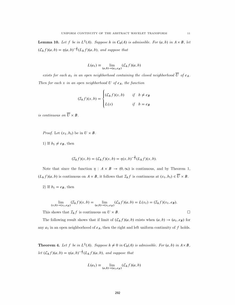
UNIFORM CONTINUITY OF THE ABSTRACT WAVELET TRANSFORM 11
Lemma 10. Let f be in L2.A/. Suppose h in C0.A/ is admissible. For .a; b/ in AB, let
.Lhf /.a; b/ D .a; b/3
2 .Lhf /.a; b/, and suppose that
L.a1/ lim.a;b/!.a1;eB /
.Lhf /.a; b/
exists for each a1 in an open neighborhood containing the closed neighborhood U of eA.
Then for each x in an open neighborhood U of eA, the function
.Ihf /.x; b/ D
8ˆ<ˆ:
.Lhf /.x; b/ if b ¤ eB
L.x/ if b D eB
is continuous on U B.
Proof. Let .x1; b1/ be in U B.
1) If b1 ¤ eB , then
.Ihf /.x; b/ D .Lhf /.x; b/ D .x; b/3
2 .Lhf /.x; b/:
Note that since the function W A B ! .0;1/ is continuous, and by Theorem 1,
.Lhf /.a; b/ is continuous on A B, it follows that Ihf is continuous at .x1; b1/ 2 U B.
2) If b1 D eB , then
lim.x;b/!.x1 ;eB /
.Ihf /.x; b/ D lim.a;b/!.x1;eB /
.Lhf /.a; b/ D L.x1/ D .Ihf /.x1; eB/:
This shows that Ihf is continuous on U B.
The following result shows that if limit of .Lhf /.a; b/ exists when .a; b/ ! .a1; eB/ for
any a1 in an open neighborhood of eA, then the right and left uniform continuity of f holds.
Theorem 4. Let f be in L2.A/. Suppose h ¤ 0 in C0.A/ is admissible. For .a; b/ in AB,
let .Lhf /.a; b/ D .a; b/3
2 .Lhf /.a; b/, and suppose that
L.a1/ lim.a;b/!.a1;eB /
.Lhf /.a; b/
292

12 JAIME NAVARRO
exists for each a1 in an open neighborhood containing the closed neighborhood U of eA. Then
if
Z
U
Z
BnV
1
Œ.a; b/3
2
dB.b/dA.a/ exists in an open neighborhood containing the closed
neighborhood V of eB, and where supp h U , then f is right and left uniformly continuous.
Proof. Since h in L2.A/ has compact support, there is an open neighborhood U of eA
such that supp h..a; b/1 x/ U , and because the inversion formula (5),
f .x/ D1
Ch
Z
U
Z
B
.Lhf /.a; b/1
.a; b/3
2
h.a; b/1 x
dB.b/dA.a/;
for the proper convergence of f , where x 2 A.
Now, we will split the integral over B into two parts so that for a closed neighborhood
V of eB ,
f .x/ D1
Ch
Z
U
Z
V
.Lhf /.a; b/1
.a; b/3
2
h.a; b/1 x
dB.b/dA.a/
C1
Ch
Z
U
Z
BnV
.Lhf /.a; b/1
.a; b/3
2
h.a; b/1 x
dB.b/dA.a/
Note that since h in L2.A/ has compact support, it follows that h is right and left
uniformly continuous (see [1]). Then for any > 0 there is a neighborhood W of eA such
that for any y 2 W and since h ı b1 is left uniformly continuous, it follows that
jf .xy/ f .x/j
1
Ch
Z
U
Z
V
j.Lhf /.a; b/j1
.a; b/3
2
ˇh.a; b/1 xy
h
.a; b/1 x
ˇdB.b/dA.a/
C1
Ch
Z
U
Z
BnV
j.Lhf /.a; b/j1
.a; b/3
2
ˇh.a; b/1 xy
h
.a; b/1 x
ˇdB.b/dA.a/
<
Ch
Z
U
Z
V
j.Lhf /.a; b/j1
.a; b/3
2
dB.b/dA.a/
C
Ch
Z
U
Z
BnV
kf k2 khk2
1
.a; b/3
2
dB.b/dA.a/
D
Ch
Z
U
Z
V
j.Ihf /.a; b/jdB .b/dA.a/
C
Ch
kf k2 khk2
Z
U
Z
BnV
1
.a; b/3
2
dB.b/dA.a/
!:
293

UNIFORM CONTINUITY OF THE ABSTRACT WAVELET TRANSFORM 13
Since Ihf is continuous on U V (see Lemma 10), and by hypothesisZ
U
Z
BnV
1
.a; b/3
2
dB.b/dA.a/ < 1, it follows that f is right uniformly continuous.
The proof for left uniformly continuous is similar.
Finally, if we drop the condition of the existence of limit of .Lhf /.a; b/ when
.a; b/ ! .a1; eB/ and instead we have that .Lhf /.a; b/ is right and left uniformly con-
tinuous, then f is right and left uniformly continuous. That is, we have the following
result.
Theorem 5. Let f be in L2.A/. Suppose h ¤ 0 in C0.A/ is admissible, and for .a; b/ in
A B, let .Lhf /.a; b/ D Œ.a; b/3
2 .Lhf /.a; b/. If .Lhf /.a; b/ is right and left uniformly
continuous on A and
Z
U
Z
BnV
1
Œ.a; b/3
2
dB.b/dA.a/ exists in an open neighborhood con-
taining the closed neighborhood V of eB , and where supp hŒ.a; b/1 x U for some closed
neighborhood U of eA, then f is right and left uniformly continuous.
Proof. Because the inversion formula (5),
f .x/ D1
Ch
Z
U
Z
B
.Lhf /.a; b/1
Œ.a; b/3
2
h.a; b/1 x
dB.b/dA.a/;
for the proper convergence of f , where x 2 A, and where supp hŒ.a; b/1 x U for
some open neighborhood containing the closed neighborhood U of eA.
Now, for a closed neighborhood V of eB , we split the integral over b 2 B into two parts
to get
f .x/ D1
Ch
Z
U
Z
V
.Lhf /.a; b/1
Œ.a; b/3
2
h.a; b/1 x
dB.b/dA.a/
C1
Ch
Z
U
Z
BnV
.Lhf /.a; b/1
Œ.a; b/3
2
h.a; b/1 x
dB.b/dA.a/:
For the first double integral, consider the change of variable w D .a; b/1 x. Then
.a; b/ w D x, which means ab.w/ D x. Hence, a D xb1.w/. Thus, dA.a/ D
dA.b1 .w// since dA is left invariant. Hence,
294
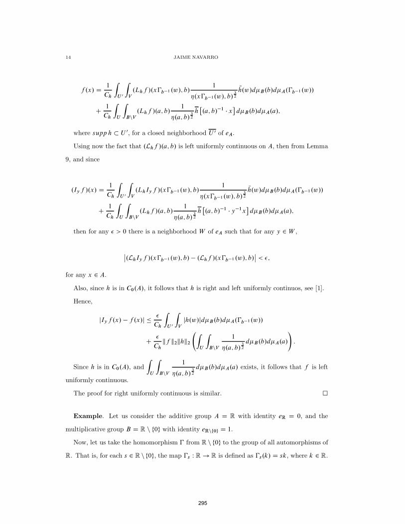
14 JAIME NAVARRO
f .x/ D1
Ch
Z
U 0
Z
V
.Lhf /.xb1 .w/; b/1
.xb1.w/; b/3
2
Nh.w/dB.b/dA.b1.w//
C1
Ch
Z
U
Z
BnV
.Lhf /.a; b/1
.a; b/3
2
h.a; b/1 x
dB.b/dA.a/;
where supp h U 0, for a closed neighborhood U 0 of eA.
Using now the fact that .Lhf /.a; b/ is left uniformly continuous on A, then from Lemma
9, and since
.Iyf /.x/ D1
Ch
Z
U 0
Z
V
.LhIyf /.xb1.w/; b/1
.xb1.w/; b/3
2
Nh.w/dB.b/dA.b1.w//
C1
Ch
Z
U
Z
BnV
.Lhf /.a; b/1
.a; b/3
2
h.a; b/1 y1x
dB.b/dA.a/;
then for any > 0 there is a neighborhood W of eA such that for any y 2 W ,
ˇ.LhIyf /.xb1.w/; b/ .Lhf /.xb1 .w/; b/
ˇ< ;
for any x 2 A.
Also, since h is in C0.A/, it follows that h is right and left uniformly continuos, see [1].
Hence,
jIyf .x/ f .x/j
Ch
Z
U 0
Z
V
jh.w/jdB.b/dA.b1.w//
C
Ch
kf k2khk2
Z
U
Z
BnV
1
.a; b/3
2
dB.b/dA.a/
!:
Since h is in C0.A/, and
Z
U
Z
BnV
1
.a; b/3
2
dB.b/dA.a/ exists, it follows that f is left
uniformly continuous.
The proof for right uniformly continuous is similar.
Example. Let us consider the additive group A D R with identity eR D 0, and the
multiplicative group B D R n f0g with identity eRnf0g D 1.
Now, let us take the homomorphism from R n f0g to the group of all automorphisms of
R. That is, for each s 2 R n f0g, the map s W R ! R is defined as s.k/ D sk, where k 2 R.
295

UNIFORM CONTINUITY OF THE ABSTRACT WAVELET TRANSFORM 15
In this case, the product in G D R R n f0g D f.k; s/jk 2 R; s 2 R n f0gg is defined as
.k; s/.k0; s0/ D .k C s.k0/; ss0/ D .k C sk0; ss0/:
Note that with this product, G becomes a locally compact topological group where the
identity is eG D .eR; eRnf0g/ D .0; 1/, and where the inverse of .k; s/ is given by
.k; s/1 D .s1 .k/; s1/ D .s1k; s1/:
Moreover, G acts on R with the following action W G R ! R given by
.k; s/ x D k C s.x/ D k C sk; where x 2 R:
On the other hand, the function W G ! .0;1/ satisfying
Z
R
h..k; s/1 x/dR.x/ D .k; s/
Z
R
h.x/dR.x/
is given by .k; s/ D jsj, where h 2 L1.R/.
Also note that the left Haar measure is given by dR.x/ D dx, and .k; s/1 x means
.k; s/1 x D .s1k; s1/ x D s1k C s1x Dx k
s:
Now, for .k; s/ 2 G define the family of two operator U.k; s/ D JkTs , where for h 2 L2.R/
1) .Jkh/.x/ D 1p.k;1/
h..k; 1/1 x/ D h.x k/; where x 2 R and k 2 R, and
2) .Tsh/.x/ D 1p.0;s/
h..0; s/1 x/ D 1pjsjh
xs
, where x 2 R and s 2 R n f0g.
Then U.k; s/ is a unitary representation of G acting on L2.R/ by
ŒU.k; s/h.x/ D .JkTsh/.x/ D .Tsh/.x k/ D1pjsjh
x k
s
:
Moreover since the left Haar measure on R n f0g is dRnf0g D 1jsjds, it follows that the
left Haar measure on G is
d.k; s/ D1
.k; s/dR.k/dRnf0g.s/ D
1
jsjdk
1
jsjds D
1
s2dkds:
296

16 JAIME NAVARRO
Then, the admissibility condition for h 2 L2.R/ becomes
Ch D
Z
Rnf0gjbh. ı s/j
2dRC.s/ D
Z
Rnf0gjbh.s/j21
sds;
where 2 R. Thus, if we take y D s, we get
Ch D
Z
Rnf0gjbh.y/j2 1
jyjdy:
Hence, for .k; s/ 2 G and h admissible in L2.R/, the continuous wavelet transform for
f 2 L2.R/ with respect to h is given by
.Lhf /.k; s/ D hf; JkTshi D
Z
R
f .x/1
jsj1
2
Nh
x k
s
dx;
and the inverse formula is given by
f D1
Ch
Z
G
.Lhf /.k; s/U.k; s/hd.k; s/;
where the equality holds in the weak sense.
1) Then because of Lemma 10 we have the following result.
Suppose f 2 L2.R/, and that h in C0.R/ is admissible. For .k; s/ in G D R RC, let
.Lhf /.k; s/ D .k; s/3
2 .Lhf /.k; s/ D s 3
2 .Lhf /.k; s/, and suppose that
L.k1/ lim.k;s/!.k1;1/
.Lhf /.k; s/
exists for each k1 in an open neighborhood containing the closed neighborhood U of 0.
Then for each x 2 U , the function
.Ihf /.x; s/ D
8ˆ<ˆ:
.Lhf /.x; s/ if s ¤ 1
L.x/ if s D 1
is continuous on U R n f0g.
This shows an example of Lemma 10.
297
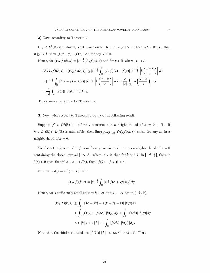
UNIFORM CONTINUITY OF THE ABSTRACT WAVELET TRANSFORM 17
2) Now, according to Theorem 2
If f 2 L2.R/ is uniformly continuous on R, then for any > 0, there is ı > 0 such that
if jyj < ı, then jf .x y/ f .x/j < for any x 2 R.
Hence, for .Whf /.k; s/ D jsj1
2 .Lhf /.k; s/ and for y 2 R where jyj < ı,
j.WhIyf /.k; s/ .Whf /.k; s/j jsj1
2
Z
R
j.Iyf /.x/ f .x/j jsj1
2
ˇˇhx k
s
ˇˇ dx
D jsj1
2
Z
R
jf .x y/ f .x/j jsj1
2
ˇˇhx k
s
ˇˇ dx <
jsj
Z
R
ˇˇhx k
s
ˇˇ dx
D
jsj
Z
R
jh .z/j jsjdz D khk1:
This shows an example for Theorem 2.
3) Now, with respect to Theorem 3 we have the following result.
Suppose f 2 L2.R/ is uniformly continuous in a neighborhood of x D 0 in R. If
h 2 L1.R/ \ L2.R/ is admissible, then lim.k;s/!.k1;1/ j.Whf /.k; s/j exists for any k1 in a
neighborhood of x D 0.
So, if > 0 is given and if f is uniformly continuous in an open neighborhood of x D 0
containing the closed interval Œ;, where > 0, then for k and k1 in Œ 2;
2, there is
ı./ > 0 such that if jk k1j < ı./, then jf .k/ f .k1/j < :
Note that if y D s1.x k/, then
.Whf /.k; s/ D jsj1
2
Z
R
jsj1
2 f .k C sy/h.y/dy:
Hence, for s sufficiently small so that k C sy and k1 C sy are in Π2;
2,
j.Whf /.k; s/j
Z
R
jf .k C sy/ f .k C sy k/j jh.y/dy
C
Z
R
jf .sy/ f .sk/j jh.y/jdy C
Z
R
jf .sk/j jh.y/jdy
< khk1 C khk1 C
Z
R
jf .sk/j jh.y/kdy:
Note that the third term tends to jf .k1/j khk1 as .k; s/ ! .k1; 1/. Thus,
298
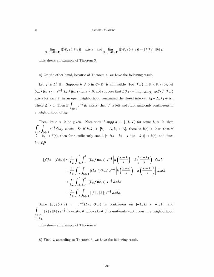
18 JAIME NAVARRO
lim.k;s/!.k1;1/
j.Whf /.k; s/j exists and lim.k;s/!.k1;1/
j.Whf /.k; s/j D jf .k1/j khk1:
This shows an example of Theorem 3.
4) On the other hand, because of Theorem 4, we have the following result.
Let f 2 L2.R/. Suppose h ¤ 0 in C0.R/ is admissible. For .k; s/ in R R n f0g, let
.Lhf /.k; s/ D s 3
2 .Lhf /.k; s/ for s ¤ 0, and suppose that L.k1/ lim.k;s/!.k1 ;1/.Lhf /.k; s/
exists for each k1 in an open neighborhood containing the closed interval Œk0 ; k0 C,
where > 0. Then if
Z
jsj>1
s 3
2 ds exists, then f is left and right uniformly continuous in
a neighborhood of k0.
Then, let > 0 be given. Note that if supp h ŒL;L for some L > 0, thenZ L
L
Z
jsj>1
s 3
2 dsdy exists. So if k; k1 2 Œk0 ; k0 C , there is ı./ > 0 so that if
jk k1j < ı./, then for s sufficiently small, js1.x k/ s1.x k1/j < ı./, and since
h 2 C10 ,
jf .k/ f .k1/j 1
Ch
Z L
L
Z 1
1
j.Lhf /.k; s/js 3
2
ˇˇhx k
s
h
x k1
s
ˇˇ dsdk
C1
Ch
Z L
L
Z
jsj>1
j.Lhf /.k; s/js 3
2
ˇˇhx k
s
h
x k1
s
ˇˇ dsdk
<
Ch
Z L
L
Z 1
1
j.Lhf /.k; s/js 3
2 dsdk
C
Ch
Z L
L
Z
jsj>1
kf k2 khk2s 3
2 dsdk:
Since .Lhf /.k; s/ D s 3
2 .Lhf /.k; s/ is continuous on ŒL;L Œ1; 1, andZ
jsj>1
kf k2 khk2 s 3
2 ds exists, it follows that f is uniformly continuous in a neighborhood
of k0.
This shows an example of Theorem 4.
5) Finally, according to Theorem 5, we have the following result.
299
UNIFORM CONTINUITY OF THE ABSTRACT WAVELET TRANSFORM 19
Suppose that f 2 L2.R/ and consider h admissible in C0.R/. For .k; s/ in
R .R n f0g/, let .Lhf /.k; s/ D s 3
2 .Lhf /.k; s/. If .Lhf /.k; s/ is uniformly continuous
on R, then f is uniformly continuous on R. To see that this result holds, choose L > 0 such
that supp h.s1.x k// ŒL;L. Then because of the inversion formula (5), the function
f can be written as
f .x/ D1
Ch
Z L
L
Z 1
1
.Lhf /.k; s/ jsj3
2 h
x k
s
ds dk
C1
Ch
Z L
L
Z
jsj>1
.Lhf /.k; s/ jsj3
2 h
x k
s
ds dk
For the first double integral consider the change of variable k D x sw. Then
f .x/ D1
Ch
Z xL
jsj
xCL
jsj
Z 1
1
.Lhf /.x sw; s/ jsj3
2 h.w/ ds .jsj/dw
C1
Ch
Z L
L
Z
jsj>1
.Lhf /.k; s/ jsj3
2 h
x k
s
ds dk
On the other hand, if .Lhf /.k; s/ is uniformly continuous on R, then for any > 0 there
is ı > 0 such that if jyj < ı, then j.Lhf /.x y sw; s/ .Lhf /.x sw; s/ < for any
x 2 R. Also, since h 2 C0.R/, it follows that h is uniformly continuous on R. Hence, for
y 2 R such that jyj < ı,
jf .x y/ f .x/j
1
Ch
Z xCL
jsj
xL
jsj
Z 1
1
j.LhIyf /.x sw; s/ .Lhf /.x sw; s/j jsj3
2 jh.w/j ds .jsj/dw
C1
Ch
Z L
L
Z
jsj>1
j.Lhf /.k; s/j jsj3
2
ˇˇhx y k
s
h
x k
s
ˇˇ ds dk:
Because of the definition of .Lhf /.k; s/, we have
jf .x y/ f .x/j
Ch
Z xCL
jsj
xL
jsj
Z 1
1
jh.w/j ds .jsj/dw
C
Ch
kf k2 khk2
Z L
L
Z
jsj>1
jsj3
2 ds dk:
Since both double integrals exist, it follows that f is uniformly continuous on R.
300
20 JAIME NAVARRO
This shows an example of Theorem 5.
References
[1] G. Folland, A course in Abstract Harmonic Analysis, CRC Press, 2000.
[2] A. Grossmann, J. Morlet, and T. Paul, Transforms associated to square integrable group representations,
I. General Results, J. Math. Phys., 26, pp. 2473-2479, (1985).
[3] J. Navarro, The Wavelet Transform of Distributions, Memorias del XXVII Congreso Nacional de la
Sociedad Matematica Mexicana, 16, pp. 145-154, (1995).
[4] J. Navarro, Use of the Wavelet Transform in Rn to find singularities of functions in L2.Rn/, Revista
Colombiana de Matematicas, Vol. 32, No.2, pp. 93-99, (1998).
[5] J. Navarro, The abstract wavelet transform, Journal of applied functional analysis, Vol. 5, pp. 266-289,
(2010).
[6] H. Reiter, Classical Harmonic Analysis and Locally Compact Groups, Oxford University Press, 2000.
301
TABLE OF CONTENTS, JOURNAL OF APPLIED FUNCTIONAL
ANALYSIS, VOL. 7, NO. 3, 2012
Impact of (E.A.) Property on Common Fixed Point Theorems in Fuzzy Metric Spaces, Jong Kyu Kim, M. S. Khan, M. Imdad and D. Gopal,…………………………………………………209
Best p-Simultaneous Approximaton in Lp(μ,X), Eyad Abu-Sirhan,……….………………..225
When an Exposed Point of a Convex Set is a Remotal Point, R. Khalil and L. Al-
Hawawsha,………………………………………………………………………………….. 236
Double Multiplier Sequence Spaces of Fuzzy Numbers Defined by a Sequence of Orlicz
Function, Kuldip Raj, Ajay K. Sharma, Anil Kumar and Sunil K. Sharma,………………... 241
Nonresonance on the Boundary and Strong Solutions of Elliptic Equations with Nonlinear Boundary Conditions, N. Mavinga and M.N. Nkashama,…………………………………...248
On Hybrid (A, η, m)-proximal Point Algorithm Frameworks for Solving General Operator Inclusion Problems, Heng-you Lan,…………………………………………………………258
On Weighted Variable Exponent Lorentz-Karamata Spaces, Ilker Eryilmaz,………………267
An Analytical Approach to the Study of the Fractal Behavior of TCP Traffic, Yingdong
Lu,…………………………………………………………………………………………...275
Uniform Continuity of the Abstract Wavelet Transform, Jaime Navarro and Salvador Arellano-Balderas,………………......................................................................................................... 282
302
Volume 7, Number 4 October 2012 ISSN:1559-1948 (PRINT), 1559-1956 (ONLINE) EUDOXUS PRESS,LLC
JOURNAL OF APPLIED FUNCTIONAL ANALYSIS
303

SCOPE AND PRICES OF
JOURNAL OF APPLIED FUNCTIONAL ANALYSIS A quartely international publication of EUDOXUS PRESS,LLC ISSN:1559-1948(PRINT),1559-1956(ONLINE) Editor in Chief: George Anastassiou Department of Mathematical Sciences The University of Memphis Memphis, TN 38152,USA E mail: [email protected] Assistant to the Editor:Dr.Razvan Mezei,Lander University,SC 29649, USA. -------------------------------------------------------------------------------- The purpose of the "Journal of Applied Functional Analysis"(JAFA) is to publish high quality original research articles, survey articles and book reviews from all subareas of Applied Functional Analysis in the broadest form plus from its applications and its connections to other topics of Mathematical Sciences. A sample list of connected mathematical areas with this publication includes but is not restricted to: Approximation Theory, Inequalities, Probability in Analysis, Wavelet Theory, Neural Networks, Fractional Analysis, Applied Functional Analysis and Applications, Signal Theory, Computational Real and Complex Analysis and Measure Theory, Sampling Theory, Semigroups of Operators, Positive Operators, ODEs, PDEs, Difference Equations, Rearrangements, Numerical Functional Analysis, Integral equations, Optimization Theory of all kinds, Operator Theory, Control Theory, Banach Spaces, Evolution Equations, Information Theory, Numerical Analysis, Stochastics, Applied Fourier Analysis, Matrix Theory, Mathematical Physics, Mathematical Geophysics, Fluid Dynamics, Quantum Theory. Interpolation in all forms, Computer Aided Geometric Design, Algorithms, Fuzzyness, Learning Theory, Splines, Mathematical Biology, Nonlinear Functional Analysis, Variational Inequalities, Nonlinear Ergodic Theory, Functional Equations, Function Spaces, Harmonic Analysis, Extrapolation Theory, Fourier Analysis, Inverse Problems, Operator Equations, Image Processing, Nonlinear Operators, Stochastic Processes, Mathematical Finance and Economics, Special Functions, Quadrature, Orthogonal Polynomials, Asymptotics, Symbolic and Umbral Calculus, Integral and Discrete Transforms, Chaos and Bifurcation, Nonlinear Dynamics, Solid Mechanics, Functional Calculus, Chebyshev Systems. Also are included combinations of the above topics. Working with Applied Functional Analysis Methods has become a main trend in recent years, so we can understand better and deeper and solve important problems of our real and scientific world. JAFA is a peer-reviewed International Quarterly Journal published by Eudoxus Press,LLC. We are calling for high quality papers for possible publication. The contributor should submit the contribution to the EDITOR in CHIEF in TEX or LATEX double spaced and ten point type size, also in PDF format. Article should be sent ONLY by E-MAIL [See: Instructions to Contributors] Journal of Applied Functional Analysis(JAFA)
is published in January,April,July and October of each year by
304

EUDOXUS PRESS,LLC, 1424 Beaver Trail Drive,Cordova,TN38016,USA, Tel.001-901-751-3553 [email protected] http://www.EudoxusPress.com visit also http://www.msci.memphis.edu/~ganastss/jafa. Webmaster:Ray Clapsadle Annual Subscription Current Prices:For USA and Canada,Institutional:Print $400,Electronic $250,Print and Electronic $450.Individual:Print $ 150, Electronic $80,Print &Electronic $200.For any other part of the world add $50 more to the above prices for Print. Single article PDF file for individual $15.Single issue in PDF form for individual $60. No credit card payments.Only certified check,money order or international check in US dollars are acceptable. Combination orders of any two from JoCAAA,JCAAM,JAFA receive 25% discount,all three receive 30% discount. Copyright©2012 by Eudoxus Press,LLC all rights reserved.JAFA is printed in USA. JAFA is reviewed and abstracted by AMS Mathematical Reviews,MATHSCI,and Zentralblaat MATH. It is strictly prohibited the reproduction and transmission of any part of JAFA and in any form and by any means without the written permission of the publisher.It is only allowed to educators to Xerox articles for educational purposes.The publisher assumes no responsibility for the content of published papers. JAFA IS A JOURNAL OF RAPID PUBLICATION
305

Journal of Applied Functional Analysis Editorial Board
Associate Editors
Editor in-Chief: George A.Anastassiou Department of Mathematical Sciences The University of Memphis Memphis,TN 38152,USA 901-678-3144 office 901-678-2482 secretary 901-751-3553 home 901-678-2480 Fax [email protected] Approximation Theory,Inequalities,Probability, Wavelet,Neural Networks,Fractional Calculus Associate Editors: 1) Francesco Altomare Dipartimento di Matematica Universita' di Bari Via E.Orabona,4 70125 Bari,ITALY Tel+39-080-5442690 office +39-080-3944046 home +39-080-5963612 Fax [email protected] Approximation Theory, Functional Analysis, Semigroups and Partial Differential Equations, Positive Operators. 2) Angelo Alvino Dipartimento di Matematica e Applicazioni "R.Caccioppoli" Complesso Universitario Monte S. Angelo Via Cintia 80126 Napoli,ITALY +39(0)81 675680 [email protected], [email protected] Rearrengements, Partial Differential Equations. 3) Catalin Badea UFR Mathematiques,Bat.M2, Universite de Lille1 Cite Scientifique F-59655 Villeneuve d'Ascq,France
23) Nikolaos B.Karayiannis Department of Electrical and Computer Engineering N308 Engineering Building 1 University of Houston Houston,Texas 77204-4005 USA Tel (713) 743-4436 Fax (713) 743-4444 [email protected] [email protected] Neural Network Models, Learning Neuro-Fuzzy Systems. 24) Theodore Kilgore Department of Mathematics Auburn University 221 Parker Hall, Auburn University Alabama 36849,USA Tel (334) 844-4620 Fax (334) 844-6555 [email protected] Real Analysis,Approximation Theory, Computational Algorithms. 25) Jong Kyu Kim Department of Mathematics Kyungnam University Masan Kyungnam,631-701,Korea Tel 82-(55)-249-2211 Fax 82-(55)-243-8609 [email protected] Nonlinear Functional Analysis,Variational Inequalities,Nonlinear Ergodic Theory, ODE,PDE,Functional Equations. 26) Robert Kozma Department of Mathematical Sciences The University of Memphis Memphis, TN 38152 USA [email protected] Neural Networks, Reproducing Kernel Hilbert Spaces, Neural Perculation Theory 27) Miroslav Krbec
306
Tel.(+33)(0)3.20.43.42.18 Fax (+33)(0)3.20.43.43.02 [email protected] Approximation Theory, Functional Analysis, Operator Theory. 4) Erik J.Balder Mathematical Institute Universiteit Utrecht P.O.Box 80 010 3508 TA UTRECHT The Netherlands Tel.+31 30 2531458 Fax+31 30 2518394 [email protected] Control Theory, Optimization, Convex Analysis, Measure Theory, Applications to Mathematical Economics and Decision Theory. 5) Carlo Bardaro Dipartimento di Matematica e Informatica Universita di Perugia Via Vanvitelli 1 06123 Perugia, ITALY TEL+390755853822 +390755855034 FAX+390755855024 E-mail [email protected] Web site: http://www.unipg.it/~bardaro/ Functional Analysis and Approximation Theory, Signal Analysis, Measure Theory, Real Analysis. 6) Heinrich Begehr Freie Universitaet Berlin I. Mathematisches Institut, FU Berlin, Arnimallee 3,D 14195 Berlin Germany, Tel. +49-30-83875436, office +49-30-83875374, Secretary Fax +49-30-83875403 [email protected] Complex and Functional Analytic Methods in PDEs, Complex Analysis, History of Mathematics. 7) Fernando Bombal Departamento de Analisis Matematico Universidad Complutense Plaza de Ciencias,3 28040 Madrid, SPAIN Tel. +34 91 394 5020 Fax +34 91 394 4726 [email protected]
Mathematical Institute Academy of Sciences of Czech Republic Zitna 25 CZ-115 67 Praha 1 Czech Republic Tel +420 222 090 743 Fax +420 222 211 638 [email protected] Function spaces,Real Analysis,Harmonic Analysis,Interpolation and Extrapolation Theory,Fourier Analysis. 28) V. Lakshmikantham Department of Mathematical Sciences Florida Institute of Technology Melbourne, FL 32901 e-mail: [email protected] Ordinary and Partial Differential Equations, Hybrid Systems, Nonlinear Analysis 29) Peter M.Maass Center for Industrial Mathematics Universitaet Bremen Bibliotheksstr.1, MZH 2250, 28359 Bremen Germany Tel +49 421 218 9497 Fax +49 421 218 9562 [email protected] Inverse problems,Wavelet Analysis and Operator Equations,Signal and Image Processing. 30) Julian Musielak Faculty of Mathematics and Computer Science Adam Mickiewicz University Ul.Umultowska 87 61-614 Poznan Poland Tel (48-61) 829 54 71 Fax (48-61) 829 53 15 [email protected] Functional Analysis, Function Spaces, Approximation Theory,Nonlinear Operators. 31) Gaston M. N'Guerekata Department of Mathematics Morgan State University Baltimore, MD 21251, USA tel:: 1-443-885-4373 Fax 1-443-885-8216 Gaston.N'[email protected] Nonlinear Evolution Equations, Abstract Harmonic Analysis, Fractional Differential Equations,
307
Operators on Banach spaces, Tensor products of Banach spaces, Polymeasures, Function spaces. 8) Michele Campiti Department of Mathematics "E.De Giorgi" University of Lecce P.O. Box 193 Lecce,ITALY Tel. +39 0832 297 432 Fax +39 0832 297 594 [email protected] Approximation Theory, Semigroup Theory, Evolution problems, Differential Operators. 9)Domenico Candeloro Dipartimento di Matematica e Informatica Universita degli Studi di Perugia Via Vanvitelli 1 06123 Perugia ITALY Tel +39(0)75 5855038 +39(0)75 5853822, +39(0)744 492936 Fax +39(0)75 5855024 [email protected] Functional Analysis, Function spaces, Measure and Integration Theory in Riesz spaces. 10) Pietro Cerone School of Computer Science and Mathematics, Faculty of Science, Engineering and Technology, Victoria University P.O.14428,MCMC Melbourne,VIC 8001,AUSTRALIA Tel +613 9688 4689 Fax +613 9688 4050 [email protected] Approximations, Inequalities, Measure/Information Theory, Numerical Analysis, Special Functions. 11)Michael Maurice Dodson Department of Mathematics University of York, York YO10 5DD, UK Tel +44 1904 433098 Fax +44 1904 433071 [email protected] Harmonic Analysis and Applications to Signal Theory,Number Theory and Dynamical Systems.
Almost Periodicity & Almost Automorphy. 32) Vassilis Papanicolaou Department of Mathematics National Technical University of Athens Zografou campus, 157 80 Athens, Greece tel:: +30(210) 772 1722 Fax +30(210) 772 1775 [email protected] Partial Differential Equations, Probability. 33) Pier Luigi Papini Dipartimento di Matematica Piazza di Porta S.Donato 5 40126 Bologna ITALY Fax +39(0)51 582528 [email protected] Functional Analysis, Banach spaces, Approximation Theory. 34) Svetlozar T.Rachev Chair of Econometrics,Statistics and Mathematical Finance School of Economics and Business Engineering University of Karlsruhe Kollegium am Schloss, Bau II,20.12, R210 Postfach 6980, D-76128, Karlsruhe,GERMANY. Tel +49-721-608-7535, +49-721-608-2042(s) Fax +49-721-608-3811 [email protected] Second Affiliation: Dept.of Statistics and Applied Probability University of California at Santa Barbara [email protected] Probability,Stochastic Processes and Statistics,Financial Mathematics, Mathematical Economics. 35) Paolo Emilio Ricci Department of Mathematics Rome University "La Sapienza" P.le A.Moro,2-00185 Rome,ITALY Tel ++3906-49913201 office ++3906-87136448 home Fax ++3906-44701007 [email protected] [email protected] Special Functions, Integral and Discrete
308

12) Sever S.Dragomir School of Computer Science and Mathematics, Victoria University, PO Box 14428, Melbourne City, MC 8001,AUSTRALIA Tel. +61 3 9688 4437 Fax +61 3 9688 4050 [email protected] Inequalities,Functional Analysis, Numerical Analysis, Approximations, Information Theory, Stochastics. 13) Paulo J.S.G.Ferreira Department of Electronica e Telecomunicacoes/IEETA Universidade de Aveiro 3810-193 Aveiro PORTUGAL Tel +351-234-370-503 Fax +351-234-370-545 [email protected] Sampling and Signal Theory, Approximations, Applied Fourier Analysis, Wavelet, Matrix Theory. 14) Gisele Ruiz Goldstein Department of Mathematical Sciences The University of Memphis Memphis,TN 38152,USA. Tel 901-678-2513 Fax 901-678-2480 [email protected] PDEs, Mathematical Physics, Mathematical Geophysics. 15) Jerome A.Goldstein Department of Mathematical Sciences The University of Memphis Memphis,TN 38152,USA Tel 901-678-2484 Fax 901-678-2480 [email protected] PDEs,Semigroups of Operators, Fluid Dynamics,Quantum Theory. 16) Heiner Gonska Institute of Mathematics University of Duisburg-Essen Lotharstrasse 65 D-47048 Duisburg Germany Tel +49 203 379 3542 Fax +49 203 379 1845 [email protected] Approximation and Interpolation Theory,
Transforms, Symbolic and Umbral Calculus, ODE, PDE,Asymptotics, Quadrature, Matrix Analysis. 36) Silvia Romanelli Dipartimento di Matematica Universita' di Bari Via E.Orabona 4 70125 Bari, ITALY. Tel (INT 0039)-080-544-2668 office 080-524-4476 home 340-6644186 mobile Fax -080-596-3612 Dept. [email protected] PDEs and Applications to Biology and Finance, Semigroups of Operators. 37) Boris Shekhtman Department of Mathematics University of South Florida Tampa, FL 33620,USA Tel 813-974-9710 [email protected] Approximation Theory, Banach spaces, Classical Analysis. 38) Rudolf Stens Lehrstuhl A fur Mathematik RWTH Aachen 52056 Aachen Germany Tel ++49 241 8094532 Fax ++49 241 8092212 [email protected] Approximation Theory, Fourier Analysis, Harmonic Analysis, Sampling Theory. 39) Juan J.Trujillo University of La Laguna Departamento de Analisis Matematico C/Astr.Fco.Sanchez s/n 38271.LaLaguna.Tenerife. SPAIN Tel/Fax 34-922-318209 [email protected] Fractional: Differential Equations-Operators- Fourier Transforms, Special functions, Approximations,and Applications. 40) Tamaz Vashakmadze I.Vekua Institute of Applied Mathematics Tbilisi State University, 2 University St. , 380043,Tbilisi, 43, GEORGIA. Tel (+99532) 30 30 40 office
309

Computer Aided Geometric Design, Algorithms. 17) Karlheinz Groechenig Institute of Biomathematics and Biometry, GSF-National Research Center for Environment and Health Ingolstaedter Landstrasse 1 D-85764 Neuherberg,Germany. Tel 49-(0)-89-3187-2333 Fax 49-(0)-89-3187-3369 [email protected] Time-Frequency Analysis, Sampling Theory, Banach spaces and Applications, Frame Theory. 18) Vijay Gupta School of Applied Sciences Netaji Subhas Institute of Technology Sector 3 Dwarka New Delhi 110075, India e-mail: [email protected]; [email protected] Approximation Theory 19) Weimin Han Department of Mathematics University of Iowa Iowa City, IA 52242-1419 319-335-0770 e-mail: [email protected] Numerical analysis, Finite element method, Numerical PDE, Variational inequalities, Computational mechanics 20) Tian-Xiao He Department of Mathematics and Computer Science P.O.Box 2900,Illinois Wesleyan University Bloomington,IL 61702-2900,USA Tel (309)556-3089 Fax (309)556-3864 [email protected] Approximations,Wavelet, Integration Theory, Numerical Analysis, Analytic Combinatorics. 21) Don Hong Department of Mathematical Sciences Middle Tennessee State University 1301 East Main St. Room 0269, Blgd KOM Murfreesboro, TN 37132-0001 Tel (615) 904-8339 [email protected] Approximation Theory,Splines,Wavelet, Stochastics, Mathematical Biology Theory.
(+99532) 30 47 84 office (+99532) 23 09 18 home [email protected] [email protected] Applied Functional Analysis, Numerical Analysis, Splines, Solid Mechanics. 41) Ram Verma International Publications 5066 Jamieson Drive, Suite B-9, Toledo, Ohio 43613,USA. [email protected] [email protected] Applied Nonlinear Analysis, Numerical Analysis, Variational Inequalities, Optimization Theory, Computational Mathematics, Operator Theory. 42) Gianluca Vinti Dipartimento di Matematica e Informatica Universita di Perugia Via Vanvitelli 1 06123 Perugia ITALY Tel +39(0) 75 585 3822, +39(0) 75 585 5032 Fax +39 (0) 75 585 3822 [email protected] Integral Operators, Function Spaces, Approximation Theory, Signal Analysis. 43) Ursula Westphal Institut Fuer Mathematik B Universitaet Hannover Welfengarten 1 30167 Hannover,GERMANY Tel (+49) 511 762 3225 Fax (+49) 511 762 3518 [email protected] Semigroups and Groups of Operators, Functional Calculus, Fractional Calculus, Abstract and Classical Approximation Theory, Interpolation of Normed spaces. 44) Ronald R.Yager Machine Intelligence Institute Iona College New Rochelle,NY 10801,USA Tel (212) 249-2047 Fax(212) 249-1689 [email protected] [email protected] Fuzzy Mathematics, Neural Networks, Reasoning, Artificial Intelligence, Computer Science.
310

22) Hubertus Th. Jongen Department of Mathematics RWTH Aachen Templergraben 55 52056 Aachen Germany Tel +49 241 8094540 Fax +49 241 8092390 [email protected] Parametric Optimization, Nonconvex Optimization, Global Optimization.
45) Richard A. Zalik Department of Mathematics Auburn University Auburn University,AL 36849-5310 USA. Tel 334-844-6557 office 678-642-8703 home Fax 334-844-6555 [email protected] Approximation Theory,Chebychev Systems, Wavelet Theory.
311
Instructions to Contributors
Journal of Applied Functional Analysis A quartely international publication of Eudoxus Press, LLC, of TN.
Editor in Chief: George Anastassiou
Department of Mathematical Sciences University of Memphis
Memphis, TN 38152-3240, U.S.A.
1. Manuscripts files in Latex and PDF and in English, should be submitted via email to the Editor-in-Chief: Prof.George A. Anastassiou Department of Mathematical Sciences The University of Memphis Memphis,TN 38152, USA. Tel. 901.678.3144 e-mail: [email protected] Authors may want to recommend an associate editor the most related to the submission to possibly handle it. Also authors may want to submit a list of six possible referees, to be used in case we cannot find related referees by ourselves. 2. Manuscripts should be typed using any of TEX,LaTEX,AMS-TEX,or AMS-LaTEX and according to EUDOXUS PRESS, LLC. LATEX STYLE FILE. (Click HERE to save a copy of the style file.)They should be carefully prepared in all respects. Submitted articles should be brightly typed (not dot-matrix), double spaced, in ten point type size and in 8(1/2)x11 inch area per page. Manuscripts should have generous margins on all sides and should not exceed 24 pages. 3. Submission is a representation that the manuscript has not been published previously in this or any other similar form and is not currently under consideration for publication elsewhere. A statement transferring from the authors(or their employers,if they hold the copyright) to Eudoxus Press, LLC, will be required before the manuscript can be accepted for publication.The Editor-in-Chief will supply the necessary forms for this transfer.Such a written transfer of copyright,which previously was assumed to be implicit in the act of submitting a manuscript,is necessary under the U.S.Copyright Law in order for the publisher to carry through the dissemination of research results and reviews as widely and effective as possible.
312

4. The paper starts with the title of the article, author's name(s) (no titles or degrees), author's affiliation(s) and e-mail addresses. The affiliation should comprise the department, institution (usually university or company), city, state (and/or nation) and mail code. The following items, 5 and 6, should be on page no. 1 of the paper. 5. An abstract is to be provided, preferably no longer than 150 words. 6. A list of 5 key words is to be provided directly below the abstract. Key words should express the precise content of the manuscript, as they are used for indexing purposes. The main body of the paper should begin on page no. 1, if possible. 7. All sections should be numbered with Arabic numerals (such as: 1. INTRODUCTION) . Subsections should be identified with section and subsection numbers (such as 6.1. Second-Value Subheading). If applicable, an independent single-number system (one for each category) should be used to label all theorems, lemmas, propositions, corollaries, definitions, remarks, examples, etc. The label (such as Lemma 7) should be typed with paragraph indentation, followed by a period and the lemma itself. 8. Mathematical notation must be typeset. Equations should be numbered consecutively with Arabic numerals in parentheses placed flush right, and should be thusly referred to in the text [such as Eqs.(2) and (5)]. The running title must be placed at the top of even numbered pages and the first author's name, et al., must be placed at the top of the odd numbed pages. 9. Illustrations (photographs, drawings, diagrams, and charts) are to be numbered in one consecutive series of Arabic numerals. The captions for illustrations should be typed double space. All illustrations, charts, tables, etc., must be embedded in the body of the manuscript in proper, final, print position. In particular, manuscript, source, and PDF file version must be at camera ready stage for publication or they cannot be considered. Tables are to be numbered (with Roman numerals) and referred to by number in the text. Center the title above the table, and type explanatory footnotes (indicated by superscript lowercase letters) below the table. 10. List references alphabetically at the end of the paper and number them consecutively. Each must be cited in the text by the appropriate Arabic numeral in square brackets on the baseline. References should include (in the following order): initials of first and middle name, last name of author(s) title of article,
313

name of publication, volume number, inclusive pages, and year of publication. Authors should follow these examples: Journal Article 1. H.H.Gonska,Degree of simultaneous approximation of bivariate functions by Gordon operators, (journal name in italics) J. Approx. Theory, 62,170-191(1990). Book 2. G.G.Lorentz, (title of book in italics) Bernstein Polynomials (2nd ed.), Chelsea,New York,1986. Contribution to a Book 3. M.K.Khan, Approximation properties of beta operators,in(title of book in italics) Progress in Approximation Theory (P.Nevai and A.Pinkus,eds.), Academic Press, New York,1991,pp.483-495. 11. All acknowledgements (including those for a grant and financial support) should occur in one paragraph that directly precedes the References section. 12. Footnotes should be avoided. When their use is absolutely necessary, footnotes should be numbered consecutively using Arabic numerals and should be typed at the bottom of the page to which they refer. Place a line above the footnote, so that it is set off from the text. Use the appropriate superscript numeral for citation in the text. 13. After each revision is made please again submit via email Latex and PDF files of the revised manuscript, including the final one. 14. Effective 1 Nov. 2009 for current journal page charges, contact the Editor in Chief. Upon acceptance of the paper an invoice will be sent to the contact author. The fee payment will be due one month from the invoice date. The article will proceed to publication only after the fee is paid. The charges are to be sent, by money order or certified check, in US dollars, payable to Eudoxus Press, LLC, to the address shown on the Eudoxus homepage. No galleys will be sent and the contact author will receive one (1) electronic copy of the journal issue in which the article appears. 15. This journal will consider for publication only papers that contain proofs for their listed results.
314
Invariant Sets for The Systems of Di¤erence Equations
Iryna Volodymyrivna Komashynska
Mathematics Department, University of Jordan, Amman 11942, Jordan, E-mail address:[email protected].
Abstract
In this work we establish the connection between the invariant sets of the systems of di¤erentialequations and the corresponding systems of di¤erence equations in terms of the zeros of positivelydenite Lyapunovs functions.Keywords:Di¤erence equations, Lyapunovs function, Invariant set, Stability.
Mathematics Subject Classication (2000): 34H05, 49J15, 93B52.
1 Introduction
The results of the existence of invariant sets for systems of di¤erential equations in terms of thezeros of non-negatively denite Lyapunovs functions have been established in the monograph ofA.M.Samoilenko [1]. Later these results were generalized for the systems of non-autonomous di¤er-ential equations and the equations with random perturbations [2],[3]. As shown in these works, thezeros of some non-negatively denite Lyapunovs function V (t; x) , t 0 , x 2 D Rm comprise aninvariant set under the condition that their projection on Rn is compact in D and the derivative ofV (t; x) with respect to the system is non-positive denite. The work [4] addressed the issue whetherthe existence of a non-negative denite Lyapunovs function is a su¢ cient condition of the existenceand stability of invariant sets. The reverse Samoilenkos theorems have been obtained, which arethe analogies of the reverse Lyapunovs theorems in the stability theory [5].
In this paper we will establish similar results for the di¤erence equations. The connectionbetween the invariant sets of the systems of di¤eretial and corresponding di¤erence equations interms of the zeros of positive denite Lyapunovs functions has been studied as well.
2 Main result
Consider the system of di¤erential equations :
dx
dt= X(t; x) (1)
and the corresponding system of di¤erence equations
xn+1 = xn +X(n; x); (2)
where n 2 Z+; x 2 D Rm. The function X(n; x) is dened forx 2 D; n 2 Z+, continuous andLipschitz with respect to x. Let M Z+ Rm; and Mn0 be the cut of M with the hyperplanen = n0; n0 2 Z+:
Denition .1 A set M is called the positively invariant set of the system (2) if the solution xn(x)of (2) such that xn(x0) 2Mn0 possesses the property: xn(x) 2Mn for n 2 Z+:
315
JOURNAL OF APPLIED FUNCTIONAL ANALYSIS, VOL.7, NO. 4,315-320,COPYRIGHT 2012 EUDOXUS PRESS,LLC
2
Denition .2 A positive invariant set M of the system (2) is called stable for n n0 if for any > 0 there exists = (; n) > 0 such that
(xn0 ;Mn0) < ;
implies(xn(x);Mn) <
for n 2 Z+;where (xn(x);Mn) = miny2Mn
kxn(x) yk is the distance of xn(x) to Mn:
Let D1 be a bounded domain, contained in D together with its neighborhood, and D1 be theclosure of D1:
Denition .3 The function V (x); dened on D1 is said to be of a sign-constant in D1 if for anyx 2 D1; the nonzero values of the function V (x) are of the same sign. A sign-constant function inD1 is called sign -denite in D1 if the set of its zeros is nonempty and compact in D1.
Denote xn(n0; x) to be the solution of the system (2) such that xn0(n0; x) = x; xn(n0; x) 2 D forany n 2 Z+:The following theorem holds.
Theorem .1 Suppose the system (2) has a positive denite stable manifold M for n 0; x 2 Dsuch that PrRmM is compact in D:
Then in some neighborhood D1 of the set M , there exists a sequence of functions Vn(x) with theproperties:
1) Vn(x) is positive denite uniformly in n 0 :
infk0;x:(x;Mk)>Vk(x) = V > 0; (3)
for any > 0 .
2) Vn(x) is negative semidenite:
Vn(x) = Vn+1(xn+1) Vn(xn) 0;
for n 0; x 2 D1 .
3) The set of zeros of Vn(x) coincides with M , that is ,
M = f(n; x) : Vn(x) = 0; n 0; x 2 D1g :
Proof. Consider the following sequence of functions
Vn(x) = supkn
2(xk(n; x);Mk);
Then
infk0;x:(x;Mk)>
Vk(x) = infk0;x:(x;Mk)>
supnk
2(xn(k; x);Mn) infk0;x:(x;Mk)>
2(xn(k; x);Mn) 2 > 0:
KOMASHYNSKA: SYSTEMS OF DIFFERENCE EQUATIONS
316

3
Thus, we haveinf
k0;x:(x;Mk)>Vk(x) = V > 0 for any > 0:
Then
4Vn(x) = Vn+1(xn+1) Vn(xn) = supkn+1
2(xk(n; x);Mk) supkn
2(xk(n; x);Mk) 0
since the second set contains more elements.To show (3) we use the fact that M is a positively stable manifold. Then for any k 0 , wehave
(xk(n; x);Mk) = 0:
Therefore Vn(x) = 0. Furthermore, if Vn(x) = 0 , then
supkn
2(xk(n; x);Mk) = 0;
so,supkn
(xk(n; x);Mk) = 0:
Then xk(n; k) 2 Mk for any k 0 , and hence M is a positively stable set.This concludes theproof of the theorem.
The further analysis is devoted to the study of the connection between the invariant sets ofthe di¤erential and the corresponding di¤erence equations. The work [4] gave the conditions on theexistence and the stability of the invariant set for the system of di¤erential equations in the terms ofthe sign constant Lyapunovs functions for the system of di¤erence equations. In the present workwe consider the reverse problem.That is, we obtain the conditions of the existence and the stabilityof an invariant set for the system of di¤erence equations in terms of the sign constant Lyapunovsfunctions for the system of di¤erential equations.
Consider an autonomous system of di¤erential equations
dx
dt= X(x) (4)
and the corresponding system of di¤erence equations
xn+1 = xn + hX(xn); (5)
where n 0; x 2 D Rm; h > 0 is the step of the di¤erence equation, and the function X(x) isbounded and Lipschitz in D.Then the following theorem holds.
Theorem .2 Suppose that there exists a positive denite smooth function V = V (x) such that@V@x is Lipschitz and
V =
V (x) =
@V (x)
@xX(x)
is non-positive denite function in D. Then the system (5) has a positive denite stable set if the
functions V (x) andV (x) are of di¤erent signs.
KOMASHYNSKA: SYSTEMS OF DIFFERENCE EQUATIONS
317
4
Proof. Suppose we have V (x) 0 andV (x) 0 for x 2
D1. It follows from ([1],p.68) that the set
V (x) = 0; x 2 D1;
is a positively invariant set for the system (4).Since V (x) is positive denite, the set of its zeros is nonempty and compact. The set of the
zeros ofV (x) is nonempty and compact as well, since
V (x) is non-positive denite in D:
Consider the following function
Vh(x) =
8<: V (x);V (x) < 0
0;V (x) = 0
9=; : (6)
Denote byNh0 = fx : Vh(x) = 0g
the set of zeros of Vh(x) .Due to the choice of Vh(x);
Nh0 = fx : V (x) = 0 g [
x :
V (x) = 0
:
Then it follows from [1, p.66] that
Nh0 = fx : Vh(x) = 0 g =
x :
V (x) = 0
:
Since V (x) 2 C1(D1), it has a derivative in any direction and at any point:
limh!0
V (x+ hX(x)) V (x)h
0
for any x 2 D1:This implies that there exists a step h0 > 0 , such that for any h < h0 the following inequality holds
4V (x) = V (x+ hX(x)) V (x) 0:
Note that we have a pointwise convergence, that is
V (x+ hX(x)) V (x)h
!V (x); as h! 0:
Now, we show that the step h0 is independent of x . Let
fh(x) =V (x+ hX(x)) V (x)
h:
Since the function V (x) is Lipschitz and X(x) is bounded, we get an estimate for jfh(x)j , that is
jfh(x)j =V (x+ hX(x)) V (x)h
= 1
hjV (x+ hX(x)) V (x)j jX(x)j C:
KOMASHYNSKA: SYSTEMS OF DIFFERENCE EQUATIONS
318

5
Moreover, since@V
@xis Lipschitz and X(x) is bounded, we get the estimate
@f
@x=
1
h
@V (x+ hX(x))
@x(I + h
@X
@x) @V (x)
@x
=
1
h
(@V (x+ hX(x))
@x @V (x)
@x) + h
@V (x+ hX(x))
@x
@X
@x)
C1:
Since h can be chosen arbitrary small,we conclude that x+ hX(x) 2 D for x 2 D1:Suppose fh(x) which satises the Lipschitz condition, is pointwise convergent and equicontinu-
ous. Then the function fh(x) is uniformly convergent,that is:
fh(x)! f(x); as h! 0;
that is, 8 > 0, 9N = N() 2 N , 8n N and 8x 2 D, we have
jfhn(x) f(x)j < :
Assume on the contrary that fh(x) is not uniformly convergent. This means that there existsan > 0 and the sequence fxng ; xn ! x0; n!1 , such that
jfhn(xn) f(xn)j :
On the other hand ,we have:
jfhn(xn) f(xn)j = jfhn(xn) fhn(x0) + fhn(x0) f(x0) + f(x0) f(xn)j jfhn(xn) fhn(x0)j+ jfhn(x0) f(x0)j+ jf(x0) f(xn)j :
Now, we give estimate of the terms in the last inequality. Since fh(x) is Lipschitz continuous,and xn ! x0; n!1; we have
jfhn(xn) fhn(x0)j L jxn x0j ! 0:
Similary, we getjf(xn) f(x0)j L jxn x0j :
But the pointwise convergence implies that the second term converges to zero, which is a contra-diction.Hence [6] implies that the system (5) has a positively invariant stable set, and the statment of thetheorem follows.
References
[1] Samoilenko.A.M. Elements of the mathematical theory of multifrequency oscillations. Moscow,Nauka, 1987.
[2] Ignatev.A.O. On the existence of a Lyapunovs function in the problem of stability of intergalsets.Ukr. Math. Jour.1993, Vol.45, No.7,PP.932-941.
[3] Stanzhytskyj.O.M. Investigation of invariant sets of systems with random perturbations byusing Lyapunovs functions.Ukr. Math.Jour.1998, Vol.50, No.2, PP.309-312.
KOMASHYNSKA: SYSTEMS OF DIFFERENCE EQUATIONS
319
6
[4] Tkachuk.A.M. Relationship between invariant sets of systems of di¤erential equations and cor-responding di¤erence equations. Nonlinear Oscillations 2006, Vol.9, No.2, PP.280-285.
[5] Demidovich.B.P. Lectures on mathematical theory of stability. Moscow, Nauka,1967.
[6] Tkachuk.A.M. Invariant sets of di¤erence systems and their stability.Nonlinear Oscillations 2005,Vol.8, No.2, PP.258-264.
[7] Ateiwi.A.M. On Reducibility of Linear Di¤erence Systems . Le Matematiche. 2007, Vol.LX11,Fasc.1, PP.41-46.
KOMASHYNSKA: SYSTEMS OF DIFFERENCE EQUATIONS
320
VORONOVSKAYA TYPE RESULT FOR q-DERIVATIVE OFq-BASKAKOV OPERATORS
ALI ARAL AND TUNCER ACAR
Abstract. The present article deals with the obtaining a Voronovskaya typeresult for q-derivative of q-Baskakov operators attached to functions in polyno-mial weighted space. For this aim, we give the central moments for q-Baskakovoperators. By using these results and some properties of q-calculus we givelimits of some central moments.
1. Introduction
Let f be a real valued function dened on [0; 1). In [2], a new q-analogue ofBaskakov operators belonging to f introduced as follows,
Bn;q(f; x) =1Xk=0
n+ k 1
k
q
qk(k1)
2xk
(1 + x)n+kq
f
[k]q
qk1[n]q
=1Xk=0
Pn;k (q; x) f
[k]qqk1[n]q
:(1.1)
where
Pn;k (q; x) =n+ k 1
k
q
qk(k1)
2xk
(1 + x)n+kq
:
for q > 0 and each positive integer n:While for q = 1 these operators coincide with the classical ones, for q 6= 1 the
new operators possess interesting properties. As in the classical Baskakov operators,the q-Baskakov operators have some shape-preserving properties and monotonicityproperty for convex function. In spite of the fact that the q-Baskakov operators arenot polynomials, they preserve the linear space of polynomials of degree m. Also,the operator Bn;q(f) becomes an approximation process, that is Bn;q(f) convergesto f uniformly on any compact subinterval of the semi-axis [0; 1) and have rateof convergence in weighted space, (see [2]). Direct global estimates for q-Baskakovoperators, using Ditzian-Totik modulus of smoothness, proved in [12]. All the abovementioned properties of these new operators motivate us for the current work.In this paper we rstly obtain a recurrence formula, including q-derivative for the
q-Baskakov operators which used to calculate q-central moment and obtain an esti-mate for the q-central moments of the q-Baskakov operators in the case q > 0. Thenusing these q-central moments, a Voronovskaya-type theorem for q-derivative of q-Baskakov operators is given. Central moment theorem for q-Bernstein operatorswas established by Videnskii [11]. These moments were generalized by Mahmudov
2000 Mathematics Subject Classication. Primary 41A25, 41A35.Key words and phrases. q-Baskakov operators, Voronovskaya-type theorem, q-derivative.
1
321
JOURNAL OF APPLIED FUNCTIONAL ANALYSIS, VOL.7, NO. 4,321-331,COPYRIGHT 2012 EUDOXUS PRESS,LLC

2 ALI ARAL AND TUNCER ACAR
[10]. The central moments and their estimates for classical linear positive oper-ators can be found [5]. Also, Voronovskaya-type theorems for derivatives of theBernstein-Chlodowsky polynomials and the Szasz-Mirakyan operators given in [7].In 2009 Aral and Gupta [3] introduced another generalization of Baskakov operatorsbased on the q-integers called q-Baskakov operators.
2. Definitions and preliminary results
Let us now recall the denition of a q-integer. Given a value of q > 0 and anynon-negative integer n, we dene [n]q as
[n]q =
(1 qn) = (1 q) ; q 6= 1n ; q = 1
:
and call [n]q a q-integer. Note that [n]q is a continuous function of q. We nextdene [n]q!, where n is a non-negative integer, as
[n]q! =
[n]q[n 1]q:::[1]q ; n = 1; 2; :::1 ; n = 0
and call [n]q! a q-factorial. The q-binomial coe¢ cientnk
is dened by
nk
q
:=[n]q!
[k]q! [n k]q!
for n k 1; and has the value 1 when k = 0 and value zero otherwise (see [1]).Note that [n]q is a polynomial in q and, less obviously,the q-binomial coe¢ cientsare also polynomials, known as Gaussian polynomials.We recall that the qderivative operator Dq is given by
(2.1) Dqf (x) :=f (qx) f (x)(q 1)x ; x 6= 0
and Dqf (x)jx=0 := f 0 (0).Higher qderivatives are
D0qf := f; Dnq f := DDn1q f
; n = 1; 2; 3; : : : :
Note that
(2.2) limq!1
Dnq f (x)) = f (n) (x) ; n = 1; 2; 3; : : : :
if f is n times di¤erentiable.The qanalogue of Leibnitz rule is
(2.3) Dq (f (x) g (x)) = g (x)Dqf (x) + f (qx)Dqg (x)
and as a symmetrically, we can write the this rule in the form
Dq (f (x) g (x)) = g (qx)Dqf (x) + f (x)Dqg (x) :
Also qderivative of a quotient is
(2.4) Dqf (x)
g (x)
=g (x)Dqf (x) f (x)Dqg (x)
g (x) g (qx):
322

q-BASKAKOV OPERATORS 3
For a 2 R, qanalogue of (a+ x)n is given by
(a+ x)nq =
n1Ys=0
(a+ qsx):
Also qderivative of (a+ x)nq is
Dq (a+ x)nq = [n]q (a+ qx)n1:
From the above denition it is obvious that a continuous function on an interval,which does not include 0 is continuous q-di¤erentiable. We say that a function fis q-di¤erentiable on a real I if for any q 2 (0; 1) the q-derivative of f exists and isnite in every x 2 I.For details see [6].
Lemma 1. ([2])For n; k 0; we have
(2.5) Dq
"xk
(1 + x)n+kq
#= [k]q
xk1
(1 + x)n+kq
qk [n+ k]qxk
(1 + x)n+k+1q
:
Lemma 2. Let m 2 N: If we dene the central moment as
Ln;m (x; q) = Bn;q((t x)mq ; x)
then we have
Ln;0 (x; q) = 1; Ln;1 (x; q) = 0; Ln;2 (x; q) =x
[n]q
1 +
1
qx
and the recurrence relations:
Ln;m+1 (qx; q) =qX
[n]qDqLn;m (x; q)
+q[m]q[n]q
xn(1 + x) x[n]q[m 1]q (1 q)2
oLn;m1 (qx; q)
+x1 q2
[m]qLn;m (qx; q) ;
where X = x (1 + x) :
Proof. It is easy to show that Ln;0 (x; q) = 1; Ln;1 (x; q) = 0; Ln;2 (x; q) = x[n]q
1 + 1
qx
by using the denition of Ln;m (x; q) : Based on (2.3) we have
DqLn;m (x; q) =1Xk=0
[m]q Pn;k (q; qx)
[k]qqk1[n]q
qxm1q
+1Xk=0
DqPn;k (q; x)
[k]qqk1[n]q
xmq
:(2.6)
From (2.5) we can write
DqPn;k (q; x) =[k]qxPn;k (q; x)
[n+ k]q(1 + x)
Pn;k (q; qx)
323
4 ALI ARAL AND TUNCER ACAR
and
x1 + qn+kx
DqPn;k (q;x) = [k]q
1 + qn+kx
Pn;k (q; x) qkx [n+ k]q Pn;k (q; x)
=[k]q xq
k [n]q
Pn;k (q; x) :
Thus
(2.7) XDqPn;k (q; x) =
[k]qqk [n]q
x![n]q Pn;k (q; qx) :
Substituting (2.7) into the (2.6), we can write:
XDqLn;m (x; q) = X1Xk=0
[m]q Pn;k (q; qx)
[k]qqk1[n]q
qxm1q
+
1Xk=0
Pn;k (q; qx) [n]q
[k]qqk1[n]q
xmq
[k]qqk [n]q
x!:
Since [k]qqk [n]q
x!=1
q
[k]q
qk1 [n]q qx qmx+ qmx
!we have
XDqLn;m (x; q) = X1Xk=0
[m]q Pn;k (q; qx)
[k]qqk1[n]q
qxm1q
+1
q
1Xk=0
Pn;k (q; qx) [n]q
[k]qqk1[n]q
xm+1q
+xqm1 1
1Xk=0
Pn;k (q; qx) [n]q
[k]qqk1[n]q
xmq
:
On the other hand, using the equality[k]q
qk1[n]q xmq
=
[k]q
qk1[n]q qx
mq
+
[k]q
qk1[n]q qx
m1q
x (qm 1)
we get
XDqLn;m (x; q) = X1Xk=0
[m]q Pn;k (q; qx)
[k]qqk1[n]q
qxm1q
+1
q
1Xk=0
Pn;k (q; qx) [n]q
[k]qqk1[n]q
qxm+1q
+1
qxqm+1 1
1Xk=0
Pn;k (q; qx) [n]q
[k]qqk1[n]q
qxmq
+xqm1 1
1Xk=0
Pn;k (q; qx) [n]q
[k]qqk1[n]q
qxmq
+x2 (qm 1)qm1 1
1Xk=0
Pn;k (q; qx) [n]q
[k]qqk1[n]q
qxm1q
:
324
q-BASKAKOV OPERATORS 5
If we rewrite the equality we have
XDqLn;m (x; q) = X [m]q Ln;m1 (qx; q) +[n]qqLn;m+1 (qx; q)
+[n]qqxqm+1 1
Ln;m (qx; q) + x
qm1 1
[n]q Ln;m (qx; q)
+x2 (qm 1)qm1 1
[n]q Ln;m1 (qx; q)
and
Ln;m+1 (qx; q) =q
[n]qXDqLn;m (x; q)
+q[m]q[n]q
xn(1 + x) x[n]q[m 1]q (1 q)2
oLn;m1 (qx; q)
+x1 q2
[m]qLn;m (qx; q) :
For m = 2 and m = 3; we have following results:Now we may present explicit formula for q-central moments of orders 3 and 4:
Corollary 1. The following equalities hold :
i) Ln;3 (x; q) = Xq
h1 + x
q (1+qq + q(1 qn)(1 + 2q + q2)
iii) Ln;4 (qx; q) = Xq
n1[n]q
+ [2]q x
1q2[n]q
(1 + q) + [3]qx
q5[n]q
+(1 + 1
q )([3]qx
2
q3 [3]qx2
q +[2]qx
q ) + [3]q xh(1 + x
q )xq (1 q
n)1 q2
i+xq (q1 q2
+1 q4
)h1 + x
q (1+qq + (1 qn)(1 + 2q + q2)
io;
where Xq = x[n]2q(1 + x
q ):
Lemma 3. Assume that qn 2 (0; 1) ; qn ! 1 and qnn ! a as n ! 1: For everyx 2 [0; 1) ; there hold
i) limn!11
qnXqn
D2qnf(x)
[2]qnLn;3 (x; qn) =
1+2x(32a)2 limn!1D2qnf (x) ;
ii) limn!11
qnXqn
D3qnf(x)
[3]qn !Ln;4 (x; qn) = x (1 + x) limn!1D3qnf (x) ;
iii) limn!11
qnXqnxq2n 1
Ln;2 (x; qn)
D2qnf(x)
[2]qn= x (1 a) limn!1D2qnf (x) ;
iv) limn!11
qnXqnxq3n 1
Ln;3 (x; qn)
D3qnf(x)
[3]qn != 0:
Proof. We only calculate i). Others are similar.i) Using the Lemma 2, it follows that
limn!1
1
qnXqn
D2qnf (x)[2]qn
Ln;3 (x; qn)
= limn!1
1
qn
D2qnf (x)[2]qn
1 +
x
qn(1 + qnqn
+ qn(1 qnn)(1 + 2qn + q2n)
=1 + 2x (3 2a)
2limn!1
D2qnf (x) :
325
6 ALI ARAL AND TUNCER ACAR
Using (2.2), we have following results:
Corollary 2. Assume that f00(x) and f
(3)
(x) exist for x 2 [0; 1) and qn 2 (0; 1); qn ! 1 and qnn ! a as n!1: For every x 2 [0; 1) ; there hold
i) limn!11
qnXqn
D2qnf(x)
[2]qnLn;3 (x; qn) =
1+2x(32a)2 f
00(x) ;
ii) limn!11
qnXqn
D3qnf(x)
[3]qn !Ln;4 (x; qn) = x (1 + x) f
(3)
(x) ;
iii) limn!11
qnXqnxq2n 1
Ln;2 (x; qn)
D2qnf(x)
[2]qn= x (1 a) f 00 (x) ;
iv) limn!11
qnXqnxq3n 1
Ln;3 (x; qn)
D3qnf(x)
[3]qn != 0:
Lemma 4. For a xed m 2 N; Bn;q((t x)mq ; x) is a polynomial in x of degree lessthan or equal to m in 1
[n]q. The minimum degree of 1
[n]qism+12
: Moreover it can
be written in the following form
Ln;m (x; q) =1
[n]bm+12 c
q
mXk=0
ak;m;n (q)xk;
Proof. By Lemma 2 it is true form = 1: Assuming that it is true. By the recurrenceformula in Lemma 2 we have
Ln;m+1 (qx; q) =qX
[n]qDq
0@ 1
[n]bm+12 c
q
mXk=0
ak;m;n (q)xk
1A+q[m]q[n]q
x(1 + x) x (1 qn)
1 qm1
Ln;m1 (qx; q)
+xq1 qm1
+1 qm+1
Ln;m (qx; q)
=qX
[n]qDq
0@ 1
[n]bm+12 c
q
mXk=0
ak;m;n (q)xk
1A+q[m]q[n]q
xn(1 + x) x [n]q [m 1]q (1 q)
2o 1
[n]bm2 c
q
m1Xk=0
ak;m1;n (q) qkxk
+x [2]q [m]q (1 q)1
[n]bm+12 c
q
mXk=0
ak;m;n (q) qkxk
326

q-BASKAKOV OPERATORS 7
and
Ln;m+1 (qx; q) =qX
[n]bm+12 c+1
q
mXk=0
ak;m;n (q) [k]q xk1
+[m]q
[n]1+bm2 cq
m1Xk=0
ak;m1;n (q) qk+1xk+1
+n1 [n]q [m 1]q (1 q)
2o [m]q
[n]1+bm2 cq
m1Xk=0
ak;m1;n (q) qk+1xk+2
+ [2]q [m]q (1 q)1
[n]bm+12 c
q
mXk=0
ak;m;n (q) qkxk+1:
Using the xq place of x we obtain
Ln;m+1 (x; q) =1
[n]bm+12 c+1
q
mXk=0
ak;m;n (q) [k]qxk
qk1
+1
[n]bm+12 c+1
q
m+1Xk=1
ak1;m;n (q) [k 1]qxk
qk1
+[m]q
[n]1+bm2 cq
mXk=1
ak1;m1;n (q)xk
+n1 [n]q [m 1]q (1 q)
2o [m]q
[n]1+bm2 cq
m+1Xk=2
ak2;m1;n (q)xk
q
+ [2]q [m]q (1 q)1
[n]bm+12 c
q
m+1Xk=1
ak1;m;n (q)xk
q
: =1
[n]bm+22 c
q
m+1Xk=0
ak;m+1;n (q)xk
ak;m+1;n (q) =1
[n] ak;m;n (q)
[k]qqk1
+1
[n] ak1;m;n (q)
[k 1]qqk1
+[m]q[n]
q
ak1;m1;n (q) +[m]qq [n]
q
n1 [n]q [m 1]q (1 q)
2oak2;m1;n (q)
+[m]qq [n]
q
[2]q (1 q) ak1;m;n (q) ;
where
a1;m;n (q) = a1;m1;n (q) = a2;m1;n (q) = 0; 0 k m+ 1;
am+1;m;n (q) = am;m1;n (q) = 0; = 1 +
m+ 1
2
m+ 2
2
= 0 or = 1:
which proves the lemma.
327
8 ALI ARAL AND TUNCER ACAR
3. Voronovskaya type theorem for q-derivatives
The following is the main convergence result of this paper. Theorem 1 is devotedto the Voronovskaya-type theorem for the q-derivative of the q-Baskakov operators.We consider the weighted space
C2 [0;1) :=f 2 C [0;1) : lim
x!1
f (x)
1 + x2uniformly continuous and bounded on [0;1)
and
Cr2 [0;1) :=f 2 C2 [0;1) : Dr
qf 2 C2 [0;1)
where C [0;1) is the space of continuous function on [0;1) : The norm in thisspace is
kfk2 := supx0
jf (x)j1 + x2
Theorem 1. Let q = qn satises 0 < qn < 1 also let qn ! 1 and qnn ! a asn!1: For each f 2 C32 [0;1) and for every x 0 we have
limn!1
[n]qn
DqnBn;qn(f;
x
qn) Dqnf (x)
qn
=1 + 2x (3 2a)
2limn!1
D2qnf (x)+x (1 + x) limn!1D3qnf (x) :
Proof. Using q-derivative, we can write
DqBn;q(f; x) = [n]q1Xk=0
qkPqn+1;k (x)f
[k + 1]qqk[n]q
f
[k]q
qk1[n]q
:
We will consider two cases. For x = 0, we have
DqBn;q(f; 0) = [n]qf
1
[n]q
f (0)
:
Since
limn!1
[n]qn
([n]qn
f
1
[n]qn
f (0)
f
0(0)
qn
)=f00(0)
2
we have desired result for x = 0:So let x > 0: By simple calculations we have
Dq1
1 + xq
n+kq
= [n+k]q
q (1 + x)n+k1q1 + x
q
n+kq
(1 + x)n+kq
= [n+ k]qq
11 + x
q
n+k+1q
:
328
q-BASKAKOV OPERATORS 9
Then by (2.3) it follows that
DqBn;q(f;x
q) =
1Xk=1
n+ k 1
k
q
qk(k1)
2 k [k]qxk1
1 + xq
n+kq
f
[k]q
qk1[n]q
1Xk=0
n+ k 1
k
q
qk(k1)
2
[n+ k]qq
xk1 + x
q
n+k+1q
f
[k]q
qk1[n]q
=1Xk=0
Pn;kq;x
q
[k]qxqk1 [n+ k]q1 + qn+k1x
!f
[k]q
qk1[n]q
:
Using the equalities
[n+ k]q = [n]q + qn [k]q
and
qk1 +
x
q
Pn;k
q;x
q
=1 + qn+k1x
Pn;k (q; x)
we can write
DqBn;q(f;x
q) =
1Xk=0
Pn;kq;x
q
[k]q xqk1 [n]qx (1 + qn+k1x)
!f
[k]q
qk1[n]q
=
1Xk=0
Pn;k (q; x)
0@ [k]q xqk1 [n]qqkx
1 + x
q
1A f [k]q
qk1[n]q
=[n]q
qx1 + x
q
1Xk=0
Pn;k (q; x)
[k]qqk1 [n]q
x!f
[k]q
qk1[n]q
=[n]q
qx1 + x
q
Bn;q((t x) f (t) ; x):(3.1)
Using the q-Taylors formula
f (t) =3Xj=0
Djqf (x)q (j + 1)
(t x)jq + (t x)3q h (t; x; q)
= f (x) + (t x)Dqf (x) + (t x) (t qx)D2qf (x)[2]q
+ (t x) (t qx)t q2x
D3qf (x)[3]q!
+ (t x)3q h (t; x; q)
we can write
(t x) f (t) = (t x) f (x) + (t x)2q Dqf (x) + x (q 1) (t x)Dqf (x)
+ (t x)3qD2qf (x)[2]q!
+ xq2 1
(t x)2q
D2qf (x)[2]q
329

10 ALI ARAL AND TUNCER ACAR
+(t x)4qD3qf (x)[3]q!
+ xq3 1
(t x)3q
D3qf (x)[3]q!
+ (t x)4q h (t; x; q) + xq3 1
(t x)3q h (t; x; q) :
where h (; x; q) 2 C32 [0;1) and limt!x h (t; x; q) = 0:Using this equality and (3.1) we have
DqBn;q(f;x
q) =
[n]q
qx1 + x
q
Bn;q((t x) f (t) ; x)=
[n]q
qx1 + x
q
Dqf (x)Ln;2 (x; q)
+[n]q
qx1 + x
q
D2qf (x)[2]q
Ln;3 (x; q) +[n]q
qx1 + x
q
x q2 1Ln;2 (x; q) D2qf (x)[2]q
+[n]q
qx1 + x
q
D3qf (x)[3]q!
Ln;4 (x; q) +[n]q
qx1 + x
q
x q3 1Ln;3 (x; q) D3qf (x)[3]q!
+[n]q
qx1 + x
q
Bn;q((t x)4q h (t; x; q) ; x) + x q3 1 [n]q
qx1 + x
q
Bn;q((t x)3q h (t; x; q) ; x); x)Since Ln;2 (x; q) = x
[n]q
1 + 1
qxwe can write
[n]q
DqBn;q(f;
x
q) Dqf (x)
q
=
[n]2q
qx1 + x
q
Dqf (x)(Ln;2 (x; q) x
[n]q
1 +
x
q
)
+[n]
2q
qx1 + x
q
D2qf (x)[2]q!
Ln;3 (x; q) +[n]
2q
qx1 + x
q
x q2 1Ln;2 (x; q) D2qf (x)[2]q!
+[n]
2q
qx1 + x
q
D3qf (x)[3]q!
Ln;4 (x; q) +[n]
2q
qx1 + x
q
x q3 1Ln;3 (x; q) D3qf (x)[3]q!
+Kn (x; q) ;
where
Kn (x; q)
=[n]
2q
qx1 + x
q
Bn;q (t x)4q h (t; x; q) ; x+ [n]2q
q1 + x
q
q3 1Bn;q (t x)3q h (t; x; q) ; x :Based on the Corollary 1, in order to complete the proof we need to show that wehave for x > 0
limn!1
Kn (x; qn) = 0:
330

q-BASKAKOV OPERATORS 11
From Cauchy -Schwarz inequality we can write
Kn (x; q)
=[n]
2q
qx1 + x
q
Bn;q (t x)4q h (t; x; q) ; x+ [n]2q
q1 + x
q
q3 1Bn;q (t x)3q h (t; x; q) ; x
qBn;q (h2 (t; x; q) ; x)
vuuut [n]4q
q2x21 + x
q
2Bn;q (t x)4q (t x)4q ; x
+qBn;q (h2 (t; x; q) ; x)
vuuut [n]4q
q21 + x
q
2 (q3 1)2Bn;q (t x)3q (t x)3q ; x:We know from [2] that
limn!1
Bn;qnh2 (t; x; qn) ; x
= 0:
We note that (t x)4q (t x)4q can be rewrite as a summation of (t x)
4q ; ::; (t x)
8q :
Using Lemma 2 we can show that the limit of[n]4qn
q2nx2(1+ x
qn)2Bn;qn
(t x)4qn (t x)
4qn; x
is nite for each x > 0: Similar situation is true for the last term of above inequality.This proves the theorem.
References
[1] G. E.Andrews, R. Askey and R. Roy, Special Functions, Cambridge Univ. Press, 1999.[2] A.Aral and V. Gupta, Generalized q Baskakov operators, Math Slovaca, (accepted)[3] A.Aral and V. Gupta, On q-Baskakov type operators, Demonstratio Math. Vol. XLII, (2009),
109-122[4] V. A. Baskakov, An example of sequence of linear positive operators in the space of continuous
functions, Dokl. Akad. Nauk. SSSR 113 (1957), 259-251.[5] Z. Ditzian and V. Totik, Moduli of Smoothness. Springer, New York (1987)[6] T. Ernst, The history of q-calculus and a new method, U.U.D.M Report 2000, 16, ISSN
1101-3591, Department of Mathematics, Upsala University, 2000.[7] P. L. Butzer and H. Karsl¬, Voronovskaya-Type Theorems for Derivatives of the Bernstein-
Chlodovsky Polynomials and the Szasz-Mirakyan Operator, Commentationes MathematicaeVol. 49, No. 1 (2009), 33-57
[8] V. Gupta and A. Aral, Generalized Baskakov-Beta operators, Rocky Mauntain Journal ofMath. (In press)
[9] V. Gupta, A note on modifed Baskakov operators, Approximation Theory Appl., 10 (3) 1994,74-78.
[10] N. Mahmudov, The moments for q-Bernstein operators in the case 0 < q < 1; Numer Algor53 (2010) ,439450.
[11] V.S. Videnskii, On some classes of q-parametric positive operators, Operator Theory Adv.Appl. 158 (2005), pp. 213222.178.
[12] Z. Finta and V. Gupta, Approximation properties of q-Baskakov operators, Cent. Eur. J.Math, 8 (2010), pp. 199-211.
K¬r¬kkale Universty, Faculty of Science and Arts, Department of Mathematics,YahSihan, K¬r¬kkale, TurkeyE-mail address : [email protected]
K¬r¬kkale Universty, Faculty of Science and Arts, Department of Mathematics,YahSihan, K¬r¬kkale, TurkeyE-mail address : [email protected]
331

SEMIGROUP ALGEBRAS AND THEIR WEAK MODULE
AMENABILITY
ABASALT BODAGHI
Abstract. In the present paper, the weak module amenability for a Banach
algebra is investigated and it is proven that for an inverse semigroup S with
the set of idempotents E, `1(S) is `1(E)-weakly module amenable. Also, itis shown that C∗(S), the enveloping C∗-algebra of `1(S), is weakly module
amenable as a C∗(E)-module with trivial left action.
1. Introduction
The concept of weak amenability was first introduced by Bade, Curtis and Dalesin [5], who termed a commutative Banach algebra A“weakly amenable” if everycontinuous derivation fromA into a symmetric BanachA-bimodule is zero. Johnsonin [13] generalized this notion for arbitrary Banach algebras and showed that forany locally compact group G, the group algebra L1(G) is weakly amenable (referto [8] for a short proof). This fact is not true for semigroups though. For instance,if C is the bicyclic inverse semigroup, then `1(C) is not weakly amenable [6].
The notion of weak module amenability of Banach algebras is defined in [4] andstudied for their second dual in [2]. The main result of [4] is that, `1(S) is weaklymodule amenable as an `1(E)-module when S is commutative. It is also proved in[2] that if E is an upward directed set and `1(E) acts on `1(S) trivially from left,then `1(S) is weakly module amenable.
In this paper, we modified the definition of the weak module amenability for aBanach algebra A which is a Banach module over Banach algebra O, and we showthat upward directed condition (the condition D1 of Duncan and Namioka [10])for E is strong and in fact, it is redundant for the inverse semigroup algebra `1(S)to be weakly module amenable as an `1(E)-module. Also, we find the relationbetween weak module amenability of A and weak amenability of A/J , where Jis the closed ideal of A generated by elements of the form (a · α)b − a(α · b), fora, b ∈ A and α ∈ O. If C∗(S) is the enveloping C∗-algebra of `1(S), then C∗(S) isweakly module amenable as a C∗(E)-module. As an example, we show that Cliffordsemigroup algebra `1(C) is `1(EC)-weakly module amenable.
2. Notations
Throughout this paper, A and O are Banach algebras such that A is a BanachO-bimodule with compatible actions, that is
α · (ab) = (α · a)b, (ab) · α = a(b · α) (a, b ∈ A, α ∈ O).
02010 Mathematics Subject Classification: Primary 46H25, 46H20; Secondary 46H35.0Keywords and phrases: Banach modules, module derivation, weak module amenability, inverse
semigroup
332
JOURNAL OF APPLIED FUNCTIONAL ANALYSIS, VOL.7, NO. 4,332-338,COPYRIGHT 2012 EUDOXUS PRESS,LLC

Let X be a Banach A-bimodule and a Banach O-bimodule with compatibleactions, that is
α·(a·x) = (α·a)·x, a·(α·x) = (a·α)·x, (α·x)·a = α·(x·a) (a ∈ A, α ∈ O, x ∈ X)
with similar actions for the right or two-sided. Then we say that X is a BanachA-O-module. If moreover
α · x = x · α (α ∈ O, x ∈ X)
then X is called a commutative A-O-module. Note that when A acts on itself byalgebra multiplication, it is not in general a Banach A-O-module, as we have notassumed the compatibility condition
a · (α · b) = (a · α) · b (α ∈ O, a, b ∈ A).
If A is a commutative O-module and acts on itself by multiplication from bothsides, then it is also a Banach A-O-module.
A bounded map D : A −→ X is called a O-module derivation if
D(α · a) = α ·D(a), D(a · α) = D(a) · αand
D(a± b) = D(a)±D(b), D(ab) = D(a) · b+ a ·D(b),
for all α ∈ O and a, b ∈ A. If X is a commutative A-O-module, then each x ∈ Xdefines a module derivation Dx(a) = a · x − x · a for all a ∈ A. These are calledthe inner module derivations. The Banach algebra A is called module amenable(as an O-module) if for any commutative Banach A-O-module X, each O-modulederivation D : A −→ X∗ is inner [1].
Consider the module projective tensor product A⊗OA which is isomorphic to thequotient space (A⊗A)/I, where I is the closed ideal of the projective tensor productA⊗A generated by elements of the form a·α⊗b−a⊗α·b for α ∈ O, a, b ∈ A [16]. Alsoconsider the closed ideal J of A generated by elements of the form (a·α)b−a(α·b) forα ∈ O, a, b ∈ A. Then I and J are A-submodules and O-submodules of A⊗A andA respectively, and the quotients A⊗OA and A/J are A-modules and O-modules.Also, A/J is a Banach A-O-modules with the compatible actions when A acts onA/J canonically.
3. Main results
Definition 3.1. The Banach algebra A is called weakly module amenable (asan O-module) if for any subset Y of A∗ which is A-submodule and commutativeBanach O-submodule, each module derivation from A to Y is inner.
In the following result, we find an equivalent definition for weak module amenabil-ity when A/J is a commutative A-O-module.
Proposition 3.2. If A/J is a commutative Banach O-module, then the followingare equivalent:
(i) Every module derivation from A to J⊥ is inner.(ii) A is weakly module amenable.Proof. (i)⇒ (ii): For each α ∈ O, a, b ∈ A, y ∈ Y , we have
〈y, (a · α)b− a(α · b)〉 = 〈y, (a · α)b〉 − 〈y, a(α · b)〉 = 〈b · y, a · α〉 − 〈y · a, α · b〉
BODAGHI: SEMIGROUP ALGEBRAS
333

= 〈α · (b ·y), a〉−〈(y ·a) ·α, b〉 = 〈(b ·y) ·α, a〉−〈α · (y ·a), b〉= 〈b · (y · α), a〉 − 〈(α · y) · a, b〉 = 〈y · α, ab〉 − 〈α · y, ab〉= 〈y · α− α · y, ab〉 = 0.
We have used the commutativity of A-submodule Y in the above equalities. Itfollows from the linearity and continuity of y as a functional on A that Y ⊆ J⊥.(ii) ⇒ (i): This follows from the fact that Y = J⊥ is a commutative Banach sub-module of A∗. ∆
Note that if O = C (the set of complex numbers), then J = 0 and so, theabove definition and Johnson’s definition [13] in the classical case for the weakamenability of Banach algebras coincide.
Let O be a commutative Banach algebra with character space ΦO and let A bea commutative Banach O-bimodule with compatible actions. Let ϕ ∈ ΦO ∪ 0.Then O is an O-bimodule with actions:
α · β = β · α = ϕ(α)β (α, β ∈ O).
Now consider the linear map ψ : A −→ O such that
ψ(ab) = ψ(a)ψ(b), ψ(a · α) = ϕ(α)ψ(a) (a ∈ A, α ∈ O).
The map ψ induces an A-module structure on O by the following action:
α · a = a · α = ϕ ψ(a)α (a ∈ A, α ∈ O).
With the above structures O becomes a commutative Banach A-O-module andwe denote it by O(ϕ,ψ). A bounded module derivation from A into O(ϕ,ψ) is calleda point module derivation on A at (ϕ,ψ).
It is proved in [7, Proposition 1.3] that if there is a non-zero, continuous pointderivation on the Banach algebra A, then it is to be failed weak amenability. Thefollowing result is its module version.
Proposition 3.3. Let A be a commutative O-module and let O be a commutativeBanach algebra. If A is weakly module amenable, then there is no non-zero boundedmodule point derivation on A.
Proof. Let ϕ and ψ be as above. By [4, Proposition 2.4] there is no non-zerobounded point derivation at (ϕ,ψ) on A when ϕ = 0. Now assume that ϕ 6= 0and d : A −→ O(ϕ,ψ) is a non-zero bounded module point derivation at (ϕ,ψ).Then the map D : A −→ A∗ defined by D(a) = d(a) · (ϕ ψ) is a bounded modulederivation because for each a, b, c ∈ A we get
〈D(ab), c〉 = 〈d(ab) · (ϕ ψ), c〉= ϕ ψ(a)ϕ ψ(c)d(b) + ϕ ψ(b)ϕ ψ(c)d(a)= 〈D(a) · b, c〉+ 〈a ·D(b), c〉.
Since D is a module derivation, there exists f ∈ A∗ such that for every a ∈ A,we have
d(a)(ϕ ψ)(a) = 〈D(a), a〉 = 〈a · f − f · a, a〉 = 〈f, a2 − a2〉 = 0.
BODAGHI: SEMIGROUP ALGEBRAS
334
Hence d = 0 on the set K = a ∈ A : ψ(a) /∈ Ker(ϕ). If a ∈ A\K and b ∈ K, then2d(ψ(a)) = d(ψ(a+b))+d(ψ(a−b)) = 0. Therefore d = 0 which is a contradiction.∆
We say that O acts trivially on A from left (right) if for each α ∈ O and a ∈ A,α · a = f(α)a (a · α = f(α)a), where f is a continuous linear functional on O. Thefollowing lemma is proved in [3, Lemma 3.1].
Lemma 3.4. Let A be a Banach algebra and Banach O-module with compatibleactions, and J0 be a closed ideal of A such that J ⊆ J0. If A/J0 has a left or rightidentity e+J0, then for each α ∈ O and a ∈ A we have a ·α−α ·a ∈ J0, i.e., A/J0is a commutative Banach O-module.
The above Lemma shows that when O acts on A trivially from left or right, thenthe actions of O on A/J from both sides are trivial, that is
α · (a+ J) = (a+ J) · α = f(α)a+ J, (a ∈ A, α ∈ O).
Thus the actions of O on A/J are trivial.
Recall that a left Banach A-module X is called a left essential A-module if thelinear span of A · X = a · x : a ∈ A, x ∈ X is dense in X. Right essentialA-modules and (two-sided) essential A-bimodules are defined similarly.
Theorem 3.5. Let A be a Banach O-module and Y be a commutative A-O-submodule of A∗, and let A/J has a left or right identity and O acts trivially on Afrom left. Consider the following statements:
(i) Every bounded derivation D : A −→ Y is inner;(ii) Every module derivation D : A −→ Y is inner;
(iii) Every module derivation D : A/J −→ Y is inner;(iv) A/J is weakly amenable;(v) A is weakly module amenable.
Then (ii) is equivalent to (iii) and (iv) is equivalent to (v). In addition, if A is aright essential O-module, then (i) implies (ii).
Proof. Since A is an essential right O-module then for each a ∈ A, there is a
sequence (En) ⊆ A·O such that limnEn = a. Suppose that En =∑Kn
m=1 an,m ·αn,mfor some finite sequences (an,m)m=Kn
m=1 ⊆ A and (αn,m)m=Knm=1 ⊆ O. Let λ ∈ C. Then
for each module derivation D : A −→ Y , we have
D(λEn) = D(λ∑Kn
m=1 an,m · αn,m) =∑Kn
m=1D(an,m · (λαn,m))
=∑Kn
m=1D(an,m) · (λαn,m) =∑Kn
m=1 λD(an,m · αn,m) = λD(En)
and so by the continuity of D, D(λa) = λD(a). Thus (i) implies (ii).(ii) ⇐⇒ (iii): The O-commutativity of Y and the compatibility of actions of Aand O on Y show that J · Y = Y · J = 0. Hence, the following module actions
(a+ J) · y := a · y, y · (a+ J) := y · a (y ∈ Y, a ∈ A),
are well-defined and so, Y is a Banach A/J-module. Assume that D : A −→ Y is
a module derivation. Define D : A/J −→ Y via D(a+ J) = D(a). For each α ∈ O
BODAGHI: SEMIGROUP ALGEBRAS
335
and a, b ∈ A we have
D((a · α)b− a(α · b)) = D((a · α)b)−D(a(α · b))= D(a · α) · b+ (a · α) ·D(b)−D(a) · (α · b)− a ·D(α · b)= (D(a) ·α) ·b−D(a) ·(α ·b)+(a ·α) ·D(b)−a ·(α ·D(b)) = 0.
On the other hand, since J is a closed ideal, the restriction of D to J is zero.
Therefore D is well-defined. By hypothesis, that is inner, and so D is inner. Now,
if D : A/J −→ Y is a module derivation, then the module derivation D : A −→ Y
defined by D(a) = D(a+ J) is inner.
(v) =⇒ (iv): Let D : A/J −→ (A/J)∗ = J⊥ and let D : A −→ J⊥ be defined by
D(a) = D(a+ J) for a ∈ A. By Lemma 3.4, for each α ∈ O and a, b ∈ A, we get
D(α · a) = D(α · a+ J) = D(f(α)a+ J) = f(α)D(a+ J) = α · D(a).
Similarly, we can obtain D(a · α) = D(a) · α. Also for a, b ∈ A we have D(a± b) =
D(a) ± D(b) and D(ab) = D(a) · b + a · D(b). Thus D is a module derivation.
Hence, there exists y ∈ Y such that D(a) = a · y − y · a. Therefore D(a + J) =(a+ J) · y − y · (a+ J) and so, D is inner.(iv) =⇒ (v): Since A/J is a O-module commutative, it is enough to prove that
each module derivation D : A −→ J⊥ is inner. Now, we define D : A/J −→ (A/J)∗
via D(a+ J) = D(a). By the proof of the part (i) =⇒ (ii), D is C-linear and thus,D is inner. ∆
One should remember that an inverse semigroup is a discrete semigroup S suchthat for each s ∈ S, there is a unique element s∗ ∈ S with ss∗s = s and s∗ss∗ = s∗.Elements of the form ss∗ are called idempotents of S and denoted by ES or E, ifthere is no risk of confusion. In this section we show that if S is an inverse semi-group with the set of idempotents E, then `1(S) is weakly module amenable (as an`1(E)-module). Suppose that S is an inverse semigroup with the set idempotentsE, endowed with the partial order
e ≤ d⇐⇒ ed = e (e, d ∈ E).
Theorem V.1.2 of [12] shows that E is a commutative subsemigroup of S . Thus`1(E) could be regarded as a subalgebra of `1(S), and thereby `1(S) is a Banachalgebra and a Banach `1(E)-module with compatible actions [1]. Here we let `1(E)acts on `1(S) by multiplication from right and trivially from left, that is
δe · δs = δs, δs · δe = δse = δs ∗ δe (s ∈ S, e ∈ E). (3.1)
In this case, the ideal J (see section 2) is the closed linear span of δset − δst :s, t ∈ S, e ∈ E. Now, we consider an equivalence relation on S as follows:
s ≈ t⇐⇒ δs − δt ∈ J (s, t ∈ S).
For an inverse semigroup S, the quotient S/≈ is a discrete group (see [3] and[14]). As in [15, Theorem 3.3], we may observe that `1(S)/J is isomorphic to`1(S/ ≈). One can see that `1(S)/J is a commutative `1(E)-bimodule with the
BODAGHI: SEMIGROUP ALGEBRAS
336
following actions:
δe · (δs + J) = δs + J, (δs + J) · δe = δse + J (s ∈ S, e ∈ E).
It is proved in [4, Theorem 3.1] that if S is a commutative inverse semigroup,then `1(S) is always weakly module amenable as an `1(E)-module when `1(E) actson `1(S) with the usual actions.
Recall that C is a Clifford semigroup if it is an inverse semigroup in which everyidempotent is central, that is es = se for all s ∈ C and e ∈ EC .
Example 3.6. Let C be a Clifford semigroup. Then `1(C) is `1(EC)-modulewith the following actions:
δe · δs = δs · δe = δes (s ∈ C, e ∈ EC).By [4, Theorem 3.1], `1(C) is weakly module amenable. Note that in the proof
of [4, Theorem 3.1], it is just used the fact that each idempotent is central.
In the upcoming theorem, we prove Amini and Bagha’s result [4, Theorem 3.1]but without the condition of commutativity for S, where we consider `1(S) as an`1(E)-module with trivial left action. In fact, we show that the hypothesis on Ebeing upward directed in [2, Corollary 3.5] can be eliminated and `1(S) is alwaysweakly module amenable.
Theorem 3.7. Let S be an inverse semigroup with the set of idempotents E.Then `1(S) is weakly module amenable.
Proof. With the actions `1(E) on `1(S) considered in (3.1), A = `1(S) is alwaysa right essential `1(E)-module. Indeed if f ∈ `1(S), we have
f =∑s∈S
f(s)δs =∑s∈S
f(s)δs ∗ δs∗s =∑s∈S
f(s)δs · δs∗s,
which belongs to the closed linear span of `1(S) · `1(E) = δs · δe : e ∈ E, s ∈ S.Since S/≈ is a discrete group, the group algebra `1(S/ ≈) has an identity. By using[8, Theorem 1] and Theorem 3.5 we can obtain the desired result. ∆
Let S be an inverse semigroup with the set of idempotents E. If C∗(S) is theenveloping C∗-algebra of `1(S) (see [9] and [11]), then by continuity of the action of`1(E) on `1(S) extends to an action of C∗(E) on C∗(S), we have the following result.
Theorem 3.8. Let S be an inverse semigroup with the set of idempotents E,then C∗(S) is weakly module amenable as a C∗(E)-module with trivial left action.
Proof. The C∗-algebra C∗(S) is weakly amenable [7, Theorem 2.1]. Also, it hasa bounded approximate identity and so, it is a right essential C∗(E)-module. Now,the result follows from the proof of the part (i) =⇒ (ii) of Theorem 3.5. ∆
Example 3.9. Let C be the bicyclic inverse semigroup generated by a and b,that is
C = ambn : m,n ≥ 0, (ambn)∗ = anbm.
The set of idempotents of C is EC = anbn : n = 0, 1, ... with the following order:
anbn ≤ ambm ⇐⇒ m ≤ n.
BODAGHI: SEMIGROUP ALGEBRAS
337
It is shown in [3] that `1(C) is `1(EC)-module amenable, and so it is weakly moduleamenable, but it is not even weakly amenable [6, Theorem 2.8].
References
[1] M. Amini, Module amenability for semigroup algebras, Semigroup Forum 69 (2004), 243–254.
[2] M. Amini and A. Bodaghi, Module amenability and weak module amenability for second dualof Banach algeras, Chamchuri J. Math. 2 (2010), no. 1, 57–71.
[3] M. Amini, A. Bodaghi and D. Ebrahimi Bagha, Module amenability of the second dual andmodule topological center of semigroup algebras, Semigroup Forum 80 (2010), 302–312.
[4] M. Amini and D. Ebrahimi Bagha, Weak module amenability for semigroup algebras, Semi-
group Forum 71 (2005), 18–26.[5] W. G. Bade, P. C. Curtis and H. G. Dales, Amenability and weak amenability for Beurling
and Lipschits algebra, Proc. London Math. Soc. (3) 55 (1987), 359–377.
[6] S. Bowling and J. Duncan, Order cohomology of Banach semigroup algebras, SemigroupForum 56 (1998), 130–145.
[7] H. G. Dales, F. Ghahramani and N. Grønbæk, Derivatios into iterated duals of Banach
algebras, Stud. Math. 128 (1) (1998), 19–54.[8] M. Despic and F. Ghahramani, Weak amenability of group algebras of locally compact groups,
Canad. Math. Bull. 37 (2)(1994), 165–167.
[9] J. Dixmier, C∗-algebras, Translated from the French by Francis Jellett, North-Holland Math-ematical Library, Vol. 15, North-Holland, Amsterdam, 1977.
[10] J. Duncan, I. Namioka, Amenability of inverse semigroups and their semigroup algebras,Proc. Roy. Soc. Edinburgh 80A (1988), 309–321.
[11] J. Duncan and A. L. T. Paterson, C∗-algebras of inverse semigroups, Proc. Roy. Soc. Edin-
burgh Soc. 28 (1985), 41–58.[12] J. M. Howie, An Introduction to Semigroup Theory, Academic Press, London, 1976.
[13] B. E. Johnson, Weak amenability of group algebras, Bull. London Math. Soc. 23 (3)(1991),
281–284.[14] H. Pourmahmood-Aghababa, (Super) Module amenability, module topological center and
semigroup algebras, Semigroup Forum, 81 (2010), 344–356.
[15] R. Rezavand, M. Amini, M. H. Sattari, and D. Ebrahimi Bagha, Module Arens regularity forsemigroup algebras, Semigroup Forum 77 (2008), 300–305.
[16] M.A.Rieffel, Induced Banach representations of Banach algebras and locally compact groups,
J. Funct. Anal. 1 (1967), 443-491.
Department of Mathematics, Islamic Azad University, Garmsar Branch, Garmsar,
Iran
E-mail address: [email protected]
BODAGHI: SEMIGROUP ALGEBRAS
338

The stability of solution for a class of third order
nonlinear vector differential equations
Muzaffer Ateş
Van Technical School, Yüzüncü Yıl University, 65080, Van –Turkey
E-mail: [email protected]
Abstract: In this paper , the stability of trivial solution for a class of third order
nonlinear vector differential equations is studied by using the Lyapunov’s second
method. Some sufficient conditions are given ensuring the stability of the zero
solution of this equation.
1. Introduction
In 2007, Yan ]1[ investigated the stability of solutions to nonlinear third order
differential equations:
0)()( =+++ xgxfxax &&&&&&
and
0)()( =+++ xgxbxfx &&&&&&& ,
and in the same year, Zhang and Si ]2[ studied asymptotic stability of the zero solution
of scalar differential equation
0)(),()( =+++ xhxxfxxgx &&&&&&& .
More recently, Tunç and Ateş ]4,3[ investigate the stability and boundedness of
solutions of non-linear vector differential equations:
),,,()()(),,( XXXtPXHXtBXXXXFX &&&&&&&&&&&& =+++
and
),,,()(),,,( XXXtPcXXGXXXXtFX &&&&&&&&&&&& =+++ ,
respectively.
________
Keywords: Stability, Lyapunov function, Differential equations of third order.
AMS (MOS) Subject Classifications: 34C11, 34D05, 34D20, 34D40.
339
JOURNAL OF APPLIED FUNCTIONAL ANALYSIS, VOL.7, NO. 4,339-344,COPYRIGHT 2012 EUDOXUS PRESS,LLC
We discusse here stability of the trivial solution 0=X of vector differential
equation of the form:
0)(),()( =+++ XHXXFXXGX &&&&&&& . )1(
The associated system of )1( is
,)(),()(
,
−−−=
==
XHYXFZYGZ
ZYYX
&
&&
)2(
where nRX ∈ , G is a continuous symmetric matrix function; F , H are −n vector
functions, ,0)0,( =XF and 0)0( =H . Let )(XJ H denote the Jacobian matrix
corresponding to the function )(XH , that is
)()( jiH xhXJ ∂∂= , ),...,2,1,( nji = ,
where ),...,,( 21 nxxx and ),...,,( 21 nhhh are the components of X and H , respectively. The
symbol ⟩⟨ YX , corresponding to any pair YX , in nR stands for the usual scalar product
∑ =
n
i ii yx1
.
It should be noted that our equation, )1( , is an −n dimensional generalization of
equation studied by Zhang and Si ]2[ .
2. Preliminaries
Before introducing our main result, we state some basic information which will
be required in future. Consider the non-autonomous differential system
),( xtFdt
dx= , )3(
where x is an n -vector, [ )∞∈ ,0t . Suppose that ),( xtF is continuous in ),( xt on DI × ,
where I denotes the interval ∞<≤ t0 and D is a connected open set in nℜ , nℜ denotes Euclidean n -space.
ATES: 3RD ORDER VECTOR DIFFERENTIAL EQUATIONS
340
Theorem 1. Suppose that 0)0,( =tF in (3) and there exists a Lyapunov function
),( xtVV = defined on ∞<≤ t0 , Hx < , 0>H , which satisfies the following
conditions;
(i) 0)0,( =tV ,
(ii) ),()( xtVxc ≤ , where CIPrc ∈)( CIP( denotesthe families of continuous
increasing and positive definite functions).
(iii) 0),( ≤xtV& .
Then, the solution 0)( ≡tx of system (3) is stable.
Proof: See Yoshizawa ]5[ .
Lemma. Let A be a real symmetric nn × -matrix. Then for any nX ℜ∈
22, XXAXX aa ∆≤⟩⟨≤δ ,
where aδ and
a∆ are respectively, the least and greatest eigenvalues of the matrix A .
Proof. See Bellman ]6[ .
3. Main result
Theorem 2. Let all the basic assumptions imposed on G , F and H hold. In
addition, we assume that there exist positive constants a and b such that the following
conditions hold:
))((2
YGa
iλ≤ , ∑∑ ==≤
n
i ii
n
i i yYXFyb
11
2),(
2 ,
abXJ Hi ≤< ))((0 λ and 0)),(( ≤XYXJ Fiλ
),...,2,1( ni = .
Then, the solution 0=X of Eq. )1( is stable.
Proof. To prove Theorem 2, we introduce a Lyapunov function ),,,( ZYXVV =
which is defined by:
⟩++⟨+⟩⟨+⟩⟨= ∫ ZaYZaYYXHdXXHaZYXV ,2
1),(),(),,(
1
0
σσ
⟩⟨−⟩⟨+ ∫ aYaYdYYYGa ,2
1,)(
1
0
σσσ ∫ ⟩⟨+
1
0
),,( σσσ dYYXF .
ATES: 3RD ORDER VECTOR DIFFERENTIAL EQUATIONS
341

This function can be rearranged as the following;
⟩⟨−⟩⟨= ∫ )(),(2
1),(),,(
1
0
XHXHb
dXXHaZYXV σσ ⟩++⟨+ )(1
),(1
2XH
bYXH
bY
b
⟩++⟨+⟩−⟨+ ∫ ZaYZaYdYIYb
YXF ,2
1),
2),((
1
0
σσσ
∫ ⟩−⟨+
1
0
,)2
)(( σσ dYYIa
YGa . )4(
It is clear from )4( that
.0)0,0,0( =V
On the other hand, since
0)0( =H , XXJXH H )()( σσσ
=∂
∂,
then
σσ XdXJXH H )()(
1
0
∫= .
By using the assumption ,))((0 abXJ Hi ≤< λ it follows that
∫ ∫ ∫ ⟩⟨=⟩⟨1
0
1
0
1
0
12211 ,)(),( σσσσσσσ ddXXXJadXXHa H
∫ ∫ =⟩⟨=⟩⟨≤
1
0
1
0
222
121 ,, XbaXXbaddXabXa σσσ
and
σσσ dXXJXXJb
XHXHb
HH∫ ⟩⟨=⟩⟨1
0
)(,)(2
1)(),(
2
1
∫ =⟩⟨≤
1
0
222
2
1,
2
1XbadXXba σ .
In view of Theorem 2 and the above discussion, we obtain
+++≥222
2
1
2
1ZaYXbaV
21 )(
2XHbY
b −+ 0≥ .
Now, let ))(),(),(( tZtYtX be any solution of system )2( .
Differentiating the function ),,( ZYXV with respect to t along system )2( , we get
ATES: 3RD ORDER VECTOR DIFFERENTIAL EQUATIONS
342

⟩⟨+⟩⟨−⟩⟨+⟩−⟨= YYXJaYYXFZaZZZYGV H ,)(),,(,,)(&
∫ ⟩⟨+
1
0
,)|),(( σσσ dYYXYXJ F .
Recall that
∫ ∫∫ ⟩⟨+⟩⟨=⟩⟨1
0
1
0
1
0
),(,)(),( σσσσσσσ dYXHdXYXJdXXHdt
dH
= ∫ ∫ ⟩⟨+⟩⟨∂
∂1
0
1
0
),(),( σσσσσ
σ dYXHdYXH
⟩⟨=⟩⟨= YXHYXH ),(),( 1
0σσ ,
∫ ∫ ⟩⟨=⟩⟨1
0
1
0
,)(,)( σσσσσσ dYZYGdYYYGdt
d
∫ ∫ ⟩⟨+⟩⟨+1
0
1
0
2 ,)(,)( σσσσσσ dZYYGdYYZYJ G
∫ ∫ ⟩⟨∂
∂+⟩⟨=
1
0
1
0
,)(,)( σσσσ
σσσσ dYZYGdYZYG
⟩⟨=⟩⟨= YZYGYZYG ,)(,)( 1
0
2 σσ
and
∫ =⟩⟨1
0
),,( σσσ dYYXFdt
d∫ ⟩⟨1
0
),,(( σσσ dZYXF
∫ ⟩⟨+
1
0
,)|),(( σσσ dYYXYXJ F ∫ ⟩⟨+
1
0
2,)|),(( σσσ dZYYYXJ F
+⟩⟨= ∫1
0
),,(( σσσ dZYXF ∫ ⟩⟨1
0
,)|),(( σσσ dYYXYXJ F
∫ ⟩⟨∂
∂+
1
0
),,( σσσ
σ dZYXF
ATES: 3RD ORDER VECTOR DIFFERENTIAL EQUATIONS
343
1
0),,( ⟩⟨= ZYXF σσ ∫ ⟩⟨+
1
0
,)|),(( σσσ dYYXYXJ F
⟩⟨= ZYXF ),,( ∫ ⟩⟨+
1
0
,)|),(( σσσ dYYXYXJ F .
In view of the assumptions of Theorem 2 and the above discussion, we get,
[ ]aYGV i −−≤ ))((λ&2
Z [ ]))(( XJab Hiλ−−2
Y
∫ ≤⟩+
1
0
0,)|),(( σσσ dYYXYXJ F .
Thus, all the conditions of Theorem 1 holds.
Then, the solution 0=X of Eq. )1( is stable.
References
[1] Cheng-zi Yan, The stability of the solution of a kind third order quasilinear
differential equation with two nonlinear terms. Chinese Journal of Engineering
Mathematics. 24 (2007), no. 2, 369-372.
[2] Zhang, L. and Si,L.,Globally asymptotic stability of a class of third order nonlinear
system. Acta Mathematicae Applicate Sinica, 30(2007), no.1, 99-103.
[3] Tunç, C. and Ateş, M., Stability and boundedness results for solutions of certain
third order nonlinear vector differential equations. Nonlinear Dynamics. 45 (2006), no. 3,
273-281.
[4] Tunç, C. and Ateş, M., Boundedness and stability of solutions to a kind of
nonlinear third order differential equations. Journal of Applied Functioal Aanalysis, 5
(2006), no. 3, 242-250.
[5] Yoshizawa, T., Stability theory by Lyapunov’s second method, The Mathematical
Society of Japan, Tokyo, 1966.
[6] Bellman, R., Introduction to matrix analysis. Reprint of the second (1970) edition.
With a foreword by Gene Golub. Classics in Applied Mathematics, 19. Society for
Industrial and Applied Mathematics (SIAM), Philadelphia, PA, 1997.
ATES: 3RD ORDER VECTOR DIFFERENTIAL EQUATIONS
344
SQUARE-MEAN ALMOST PERIODIC SOLUTIONS TO SOMECLASSES OF NONAUTONOMOUS STOCHASTIC
EVOLUTION EQUATIONS WITHFINITE DELAY
PAUL BEZANDRY AND TOKA DIAGANA
Abstract. In this paper, using the well-known Krasnoselskii fixed point theo-
rem, we obtain the existence of a square-mean almost periodic solution to some
classes of nonautonomous stochastic evolution equations with finite delay.
1. Introduction
Let (H, ‖·‖, 〈·, ·〉) be a real separable Hilbert space and let (Ω,F ,P) be a completeprobability space equipped with a normal filtration Ft : t ∈ R, that is, a right-continuous, increasing family of sub σ-algebras of F .
In recent years, the existence of almost periodic (respectively, periodic) solutionsto semilinear evolution equations has received much attention by many authors (see,e.g. [3], [8], [16], and [33] and the references therein) due to their significance andapplications in physics, mathematical biology, control theory, and others. Thisinterest also arises from a need to extend well-known results on stochastic ordinarydifferential equations to a class of stochastic partial differential equations.
In their recent paper [9], the authors studied the existence of square-mean almostperiodic solutions to the class of nonautonomous stochastic differential equations
dX(t) = A(t)X(t) dt + M(t, X(t)) dt + N(t, X(t)) dW(t), t ∈ R,(1.1)
where (A(t))t∈R is a family of densely defined closed linear operators, M : R ×L2(Ω, H) → L2(Ω, H) and N : R × L2(Ω, H) → L2(Ω, L0
2) are jointly continu-ous satisfying some additional conditions, and W is a Wiener process. For that,Bezandry and Diagana assumed that the family of linear operators A(t) satisfythe well-known Acquistapace-Terreni conditions [3], which in fact do guarantee theexistence of an evolution family T = V (t, s)t≥s associated with the family of lin-ear operators A(t). The main result in [9] was then subsequently utilized to studythe existence of square-mean almost periodic solutions to some parabolic stochasticpartial differential equations.
In this paper, our approach to this problem is somewhat different from thatused in [9]. We consider a more general setting, that is, we make extensive use ofintermediate space techniques and the Krasnoselskii fixed point theorem to studyand obtain the existence of square-mean almost periodic solutions to the class of
1991 Mathematics Subject Classification. 34K50; 35R60; 43A60; 34B05; 34C27; 42A75; 47D06;
35L90.Key words and phrases. stochastic evolution equation; stochastic processes; square-mean al-
most periodic; Wiener process; sectorial operator; evolution family; exponential dichotomy; Ac-quistapace and Terreni conditions; Krasnoselskii fixed point theorem.
1
345
JOURNAL OF APPLIED FUNCTIONAL ANALYSIS, VOL.7, NO. 4,345-366,COPYRIGHT 2012 EUDOXUS PRESS,LLC

2 PAUL BEZANDRY AND TOKA DIAGANA
nonautonomous stochastic differential equations with finite delay given by
(1.2) d[X(t) + F1(t, Xt)
]= A(t)X(t)dt + F2(t, Xt)dt + F3(t, Xt)dW(t)
where (A(t))t∈R is a family of closed linear operators on H satisfying Acquistapace-Terreni conditions, the history Xt defined by Xt(θ) := X(t+θ) for each θ ∈ [−τ, 0],and the functions F1 : R × L2(Ω, Cτ ) → L2(Ω, Ht
β) (0 ≤ α < 0.5 < β < 1),Fi(i = 2, 3) : R × L2(Ω, Cτ ) 7→ L2(Ω, H) are jointly continuous satisfying someadditional conditions, and W is a R-valued Brownian motion with the real numberline as time parameter. (Here Ht
β is an interpolation space and for 0 ≤ α < 1,Cτ, α := C([−τ, 0], Hα) is the Banach space of all continuous functions from [−τ, 0]in Hα.)
In view of the above, there exists an evolution family U = U(t, s)t≥s associ-ated with the family of closed linear operators A(t). Assuming that the evolutionfamily U = U(t, s)t≥s is exponentially dichotomic (hyperbolic) and under someadditional assumptions, it will be shown that Eq. (1.2) has a square-mean al-most periodic solution. It is worth mentioning that the main result of this papergeneralizes, to some extent, most of known results on square-mean almost peri-odic solutions to autonomous and nonautonomous differential equations, especiallythose in [8], [9], and [10].
The paper is organized as follows: Section 2 is devoted to preliminaries factsrelated to the existence of an evolution family. Some preliminary results on in-termediate spaces are also stated there. In Section 3, basic definitions and resultson the concept of square-mean almost periodic functions are given. In Section 4,we first state a key technical lemma due to Diagana [14] and next make use ofit to prove the main result. In Section 5, we illustrate our main result by study-ing the existence of square-mean almost periodic solutions to the one-dimensionalstochastic heat equation with finite delay.
2. Preliminaries
In this section, we introduce some notations and collect some preliminary resultsfrom Diagana [14] that will be used later. Throughout the rest of this paper,(H, ‖ · ‖, 〈·, ·〉) stands for a real separable Hilbert space, A(t) for t ∈ R is a familyof closed operators on D(A(t)) satisfying the Acquistapace-Terreni conditions (see(H.1)). Moreover, the operators A(t) are not necessarily densely defined. Thefunctions F1 : R×Cτ → Ht
β (0 ≤ α < 0.5 < β < 1), and Fi(i = 2, 3) : R×Cτ → Hare respectively jointly continuous satisfying some additional assumptions.
If L is a linear operator on H, then ρ(L), σ(L), D(L), ker(L), R(L) stand respec-tively for the resolvent set, spectrum, domain, kernel, and range of L. Moreover,one sets R(λ, L) = (λI − L)−1 for all λ ∈ ρ(L).
Throughout the rest of the paper, we set Q(t) = I − P (t), if P (t) is a family ofprojections. If B1, B2 are Banach spaces, then the notation B(B1, B2) stands forthe Banach space of bounded linear operators from B1 into B2. When B1 = B2,this is simply denoted B(B1).
In the present work we study operators A(t) on H subject to the followinghypotheses.Hypothesis (H.1). The family of closed linear operators A(t) for t ∈ R on Hwith domain D = D(A(t)) (possibly not densely defined) satisfy the so-called Ac-quistapace and Terreni conditions, that is:
346

SQUARE-MEAN ALMOST PERIODIC SOLUTIONS 3
there exist constants ζ ∈ R, θ ∈ (π2 , π), L > 0 and µ, ν ∈ (0, 1] with µ + ν > 1 such
that
Σθ ∪0⊂ ρ(A(t)− ζ) 3 λ,
∥∥∥R(λ,A(t)− ζ
)∥∥∥ ≤ K
1 + |λ|(2.1)
and ∥∥∥(A(t)− ζ
)R
(λ,A(t)− ζ
)[R
(ζ,A(t)
)−R
(ζ,A(s)
)]∥∥∥ ≤ L∣∣t− s
∣∣µ∣∣λ∣∣−ν(2.2)
for t, s ∈ R, λ ∈ Σθ :=
λ ∈ C\0 :∣∣argλ
∣∣ ≤ θ
.In the particular case when A(t) has a constant domain D = D(A(t)), Eq. (2.2)
can be replaced with the following: there exist constants L and 0 < µ ≤ 1 suchthat ∥∥∥(
A(t)−A(s))R
(ζ,A(r)
)∥∥∥ ≤ L∣∣t− s
∣∣µ, s, t, r ∈ R.
It should be mentioned that (H.1) was introduced in the literature by Acquistapaceand Terreni [3] for ζ = 0. Among other things, it ensures that there exists a uniqueevolution family U = U(t, s) on H satisfying
(a) U(t, s)U(s, r) = U(t, r) for t ≥ s ≥ r ∈ R;(b) U(t, t) = I(c) (t, s) → U(t, s) ∈ B(H) is continuous for t > s;
(d) U(·, s) ∈ C1((s,∞), B(H)),∂U
∂t(t, s) = A(t)U(t, s) and
∥∥A(t)kU(t, s)∥∥ ≤
C(t− s)−k for 0 < t− s ≤ 1, k = 0, 1; and(e) ∂+
s U(t, s)x = −U(t, s)A(s)x for t > s and x ∈ D(A(s)) with A(s)x ∈D(A(s).
It should also be mentioned that the above-mentioned properties were mainlyestablished in [1, Theorem 2.3] and [35, Theorem 2.1], see also [3, 34]. In this casewe say that A(·) generates the evolution family U(·, ·).
Definition 2.1. We say that an evolution family U(t, s) has an exponential di-chotomy (or is hyperbolic) if there are projections P (t), t ∈ R, being uniformlybounded and strongly continuous in t and constants δ > 0 and N ≥ 1 such that
(1) U(t, s)P (s) = P (t)U(t, s),(2) the restriction UQ(t, s) : Q(s)H → Q(t)H of U(t, s) is invertible (and we set
UQ(s, t) := UQ(t, s)−1),(3)
∥∥U(t, s)P (s)∥∥ ≤ Ne−δ(t−s) and
∥∥UQ(s, t)Q(t)∥∥ ≤ Ne−δ(t−s) for t ≥ s and
t, s ∈ R.
Here and below Q = I − P for a projection P . Under Acquistpace-Terreniconditions, the family of operators defined by
Γ(t, s) =
U(t, s)P (s), if t ≥ s, t, s ∈ R
−UQ(t, s)Q(s), if t < s, t, s ∈ R
are called Green function corresponding to U and P (·). If P (t) = I for t ∈ R, thenU is exponentially stable.
This setting requires some estimates related to U(t, s). For that, we introducethe interpolation spaces for A(t). For details, we refer the reader to Lunardi [24].
347
4 PAUL BEZANDRY AND TOKA DIAGANA
Definition 2.2. A linear operator A : D(A) ⊂ H → H (not necessarily denselydefined) is said to be sectorial if the following hold: there exist constants ζ ∈ R,θ ∈
(π
2, π
), and M > 0 such that Sθ,ζ ⊂ ρ(A),
Sθ,ζ :=λ ∈ C : λ 6= ζ,
∣∣arg(λ− ζ)∣∣ < θ
and
∥∥R(λ,A)∥∥ ≤ M∣∣λ− ζ
∣∣ , λ ∈ Sθ,ζ
where R(λ,A) = (λI −A)−1 for each λ ∈ ρ(A).
LetA be a sectorial operator on H and let α ∈ (0, 1). Define the real interpolationspace
HAα :=
x ∈ H :∥∥x
∥∥Aα
:= supr>0
∥∥rα(A− ζ)R(r,A− ζ)x∥∥ < ∞
,
which is a Banach space when endowed with the norm∥∥ · ∥∥A
α. For convenience we
further write
HA0 := H,∥∥x
∥∥A0
:=∥∥x
∥∥, HA1 := D(A) and∥∥x
∥∥A1
:=∥∥(ζ −A)x
∥∥.
Moreover, let HA := D(A) of H. In particular, we will frequently be using thefollowing continuous embedding
D(A) → HAβ → D((ζ −A)α
)→ HAα → HA ⊂ H,(2.3)
for all 0 < α < β < 1, where the fractional powers are defined in the usual way.In general, D(A) is not dense in the spaces HAα and H. However, we have the
following continuous injection
HAβ → D(A)
∥∥·∥∥Aα(2.4)
for 0 < α < β < 1.Given the family of linear operators A(t) for t ∈ R, satisfying (H.1), we set
Htα := HA(t)
α , Ht := HA(t)
for 0 ≤ α ≤ 1 and t ∈ R, with the corresponding norms.The embedding in (2.3) hold with constants independent of t ∈ R. These inter-
polation spaces are of class Jα (see [24]) and hence there is a constant c(α) suchthat ∥∥y
∥∥t
α≤ c(α)
∥∥y∥∥1−α∥∥A(t)y
∥∥α, y ∈ D(A(t)).(2.5)
we have the following estimates for the evolution family U .
Lemma 2.3. [7, 14] For x ∈ H, 0 ≤ α ≤ 1, and t > s, the following hold
(i) There is a constant c(α) such that∥∥∥U(t, s)P (s)x∥∥∥t
α≤ c(α)e−
δ2 (t−s)(t− s)−α
∥∥x∥∥.(2.6)
(ii) There is a constant m(α) such that∥∥∥UQ(s, t)Q(s)x∥∥∥s
α≤ m(α)e−δ(t−s)
∥∥x∥∥.(2.7)
348

SQUARE-MEAN ALMOST PERIODIC SOLUTIONS 5
In addition to above, we also need the following assumptions:Hypothesis (H.2). The domain D(A(t) = D is constant in t ∈ R. Moreover, theevolution family U generated by A(·) has an exponential dichotomy with constantsN , δ > 0 and dichotomy projections P (t) for t ∈ R. Furthermore, 0 ∈ ρ(A(t)) foreach t ∈ R and the following holds
supt, s∈R
∥∥∥A(s)A−1(t)∥∥∥
B(H,Hα)< c0 .(2.8)
If 0 ≤ µ < α < β < 1, then the nonnegative constants k(α), k, k′,, and k2 denoterespectively the bounds of the embedding Hβ → Hα, Hα → H, Hβ → H, andHµ → H.
3. Square-Mean Almost periodic Stochastic Processes
For details on this section, we refer the reader to [8, 11] and the referencestherein. In this paper, we assume that (Ω,F ,P) is a probability space. Let W be aBrownian motion on R. It is worth mentioning that W can be obtained as follows:let Wi(t), t ∈ R+, i = 1, 2, be independent R-valued Brownian motions, then
W(t) =
W1(t) if t ≥ 0,
W2(−t) if t ≤ 0,
is a Brownian motion with the real number line as time parameter. We then letFt = σW(s), s ≤ t.
Let (B, ‖ · ‖) be a Banach space. This setting requires the following preliminarydefinitions.
Definition 3.1. A stochastic process X : R → L2(Ω; B) is said to be continuouswhenever
limt→s
E∥∥∥X(t)−X(s)
∥∥∥2
= 0.
Definition 3.2. A continuous stochastic process X : R → L2(Ω; B) is said to besquare-mean almost periodic if for each ε > 0 there exists l(ε) > 0 such that anyinterval of length l(ε) contains at least a number τ for which
supt∈R
E∥∥∥X(t + τ)−X(t)
∥∥∥2
< ε.
The collection of all stochastic processes X : R → L2(Ω; B) which are quadraticmean almost periodic is then denoted by AP (R; L2(Ω; B)).
The next lemma provides some properties of square-mean almost periodic pro-cesses.
Lemma 3.3. If X belongs to AP (R;L2(Ω; B)), then
(i) the mapping t → E∥∥X(t)
∥∥2 is uniformly continuous;(ii) there exists a constant M > 0 such that E
∥∥X(t)∥∥2 ≤ M , for all t ∈ R.
Let CUB(R; L2(Ω; B)) denote the collection of all stochastic processes X : R →L2(Ω; B), which are continuous and uniformly bounded. It is then easy to checkthat CUB(R; L2(Ω; B)) is a Banach space when it is equipped with the norm:∥∥X
∥∥∞ = sup
t∈R
(E‖X(t)‖2
) 12.
349

6 PAUL BEZANDRY AND TOKA DIAGANA
Lemma 3.4. AP (R; L2(Ω; B)) ⊂ CUB(R; L2(Ω; B)) is a closed subspace.
In view of the above, the space AP (R; L2(Ω; B)) of square-mean almost periodicprocesses equipped with the norm
∥∥ · ∥∥∞ is a Banach space.Let (B1,
∥∥·∥∥B1) and (B2,
∥∥·∥∥B2) be Banach spaces and let L2(Ω; B1) and L2(Ω; B2)
be their corresponding L2-spaces, respectively.
Definition 3.5. A function F : R × L2(Ω; B1) → L2(Ω; B2)), (t, Y ) 7→ F (t, Y ),which is jointly continuous, is said to be square-mean almost periodic in t ∈ Runiformly in Y ∈ K where K ⊂ L2(Ω; B1) is any compact subset if for any ε > 0,there exists l(ε, K) > 0 such that any interval of length l(ε, K) contains at least anumber τ for which
supt∈R
E∥∥∥F (t + τ, Y )− F (t, Y )
∥∥∥2
B2
< ε
for each stochastic process Y : R → K.
Theorem 3.6. Let F : R× L2(Ω; B1) → L2(Ω; B2), (t, Y ) 7→ F (t, Y ) be a square-mean almost periodic process in t ∈ R uniformly in Y ∈ K, where K ⊂ L2(Ω; B1)is compact. Suppose that F is Lipschitz in the following sense:
E∥∥∥F (t, Y )− F (t, Z)
∥∥∥2
B2
≤ M E∥∥∥Y − Z
∥∥∥2
B1
for all Y, Z ∈ L2(Ω; B1) and for each t ∈ R, where M > 0. Then for any square-mean almost periodic process Φ : R → L2(Ω; B1), the function t 7→ F (t,Φ(t)) issquare-mean almost periodic.
The present setting requires the following composition of square-mean almostperiodic processes.
Theorem 3.7. Let F : R× L2(Ω; B1) → L2(Ω; B2), (t, Y ) 7→ F (t, Y ) be a square-mean almost periodic process in t ∈ R uniformly in Y ∈ K, where K ⊂ L2(Ω; B1)is any compact subset. Suppose that F (t, ·) is uniformly continuous on boundedsubsets K ′ ⊂ L2(Ω; B1) in the following sense: for all ε > 0 there exists δε > 0 such
that X, Y ∈ K ′ and E∥∥∥X − Y
∥∥∥2
B1
< δε, then
E∥∥∥F (t, X)− F (t, Y )
∥∥∥2
B2
< ε, ∀t ∈ R.
Then for any square-mean almost periodic process Φ : R → L2(Ω; B1), the functiont 7→ F (t,Φ(t)) is square-mean almost periodic.
Proof. Since Φ : R → L2(Ω; B1) is a square-mean almost periodic process, for allε > 0 there exists lε > 0 such that every interval of length lε > 0 contains a τ withthe property that
E∥∥∥Φ(t + τ)− Φ(t)
∥∥∥2
B1
< ε, ∀t ∈ R.(3.1)
In addition, Φ : R → L2(Ω; B1) is bounded, that is, supt∈R
E∥∥∥Φ(t)
∥∥∥2
B1
< ∞. Let
K ′′ ⊂ L2(Ω; B1) be a bounded subset such that Φ(t) ∈ K ′′ for all t ∈ R.Now
350
SQUARE-MEAN ALMOST PERIODIC SOLUTIONS 7
E∥∥∥F (t + τ,Φ(t + τ))− F (t,Φ(t))
∥∥∥2
B2
≤ 2E∥∥∥F (t + τ,Φ(t + τ))− F (t + τ,Φ(t))
∥∥∥2
B2
+ 2E∥∥∥F (t + τ,Φ(t))− F (t,Φ(t))
∥∥∥2
B2
.
Taking into account Eq. (3.1) (take δε = ε) and using the uniform continuity of Fon bounded subsets of L2(Ω; B1) it follows that
supt∈R
E∥∥∥F (t + τ,Φ(t + τ))− F (t + τ,Φ(t))
∥∥∥2
B2
<ε
4.(3.2)
Similarly, using the square-mean almost periodicity of F it follows that
supt∈R
E∥∥∥F (t + τ,Φ(t))− F (t,Φ(t))
∥∥∥2
B2
<ε
4.(3.3)
Combining Eq. (3.2) and Eq. (3.3) one obtains that
supt∈R
E∥∥∥F (t + τ,Φ(t + τ))− F (t,Φ(t))
∥∥∥2
B2
< ε,
and hence the function t 7→ F (t,Φ(t)) is square-mean almost periodic.
4. Existence of Square-Mean Almost Periodic Solutions
This section is devoted to the existence of a square-mean almost periodic solutionto the nonautonomous stochastic differential equation Eq. (1.2).
In the sequel, we denote for brevity that for 0 ≤ α < 1, Cτ, α = C([−τ, 0], Hα),the space of all continuous functions from [−τ, 0] into Hα, equipped with the supnorm given by ∥∥z
∥∥τ, α
:=[
sup−τ≤θ≤0
∥∥z(θ)∥∥2
α
]1/2
.
Definition 4.1. A continuous random function, X : R 7→ L2(Ω; Cτ, α) is said tobe a bounded solution of Eq.(1.2) on R provided that s → A(s)Γ(t, s)F1(s,Xs) isintegrable on (−∞, t) and, s → A(s)Γ(t, s)F1(s,Xs) is integrable on (t,∞), and
X(t) = −F1(t, Xt)−∫ t
−∞A(s)Γ(t, s) F1(s,Xs) ds +
∫ ∞
t
A(s)Γ(t, s) F1(s,Xs) ds
+∫ t
−∞Γ(t, s) F2(s,Xs) ds−
∫ ∞
t
Γ(t, s) F2(s,Xs) ds
+∫ t
−∞Γ(t, s) F3(s,Xs) dW(s)−
∫ ∞
t
Γ(t, s) F3(s,Xs) dW(s)
for each t ≥ s and for all t, s ∈ R.
In this paper, Γ1, Γ2, Γ3, Γ4, Γ5, and Γ6 stand respectively for the nonlinearintegral operators defined by
(Γ1X)(t) :=∫ t
−∞A(s)Γ(t, s) Ψ1(s) ds, (Γ2X)(t) :=
∫ ∞
t
A(s)Γ(t, s) Ψ1(s) ds,
(Γ3X)(t) :=∫ t
−∞Γ(t, s) Ψ2(s) ds, (Γ4X)(t) :=
∫ ∞
t
Γ(t, s) Ψ2(s) ds,
351
8 PAUL BEZANDRY AND TOKA DIAGANA
(Γ5X)(t) :=∫ t
−∞Γ(t, s) Ψ3(s) dW(s), (Γ6X)(t) :=
∫ ∞
t
Γ(t, s) Ψ3(s) dW(s),
where Ψ1(s) = F1(s,Xs), Ψ2(s) = F2(s,Xs), and Ψ3(s) = F3(s,Xs).To discuss the existence of square-mean almost periodic solution to Eq. (1.2) we
need some additional assumptions. First of all, note that for 0 < α < β < 1, then
L2(Ω, Hβ) → L2(Ω, Hα) → L2(Ω; H)
are continuously embedded and hence therefore exist constants k1 > 0, k(α) > 0such that
E∥∥X
∥∥2 ≤ k1E∥∥X
∥∥2
αfor each X ∈ L2(Ω, Hα) and
E∥∥X
∥∥2
α≤ k(α)E
∥∥X∥∥2
βfor each X ∈ L2(Ω, Hβ).
(H.3) R(ζ,A(·)) ∈ B(AP (R;L2(Ω; Hα))
). Moreover, there exists a function γ :
[0,∞) → [0,∞) with γ ∈ L1[0,∞) such that for every ε > 0 there existsl(ε) such that every interval of length l(ε) contains a τ with the property∥∥∥A(t + τ)Γ(t + τ, s + τ)−A(t)Γ(t, s)
∥∥∥B(Hα,H)
≤ εγ(∣∣t− s
∣∣)for all s, t ∈ R.
(H.4) Let 0 ≤ α < 0.5 < β < 1. Let F1 : R×L2(Ω;Cτ,α) → L2(Ω, Hβ) be square-mean almost periodic in t ∈ R uniformly in X ∈ O (O ⊂ L2(Ω;Cτ,α) beingany compact subset). Moreover, F1 is Lipschitz in the following sense: thereexists K1 > 0 for which
E∥∥∥F1(t, X)− F1(t, Y )
∥∥∥2
β≤ K1 E
∥∥∥X − Y∥∥∥2
τ,α
for all random variables X, Y ∈ L2(Ω;Cτ,α) and t ∈ R;(H.5) Let Fi(i = 2, 3) : R × L2(Ω; Cτ,α) → L2(Ω, H) be square-mean almost
periodic in t ∈ R uniformly in X ∈ Oi (Oi ⊂ L2(Ω; Cτ,α)) being anycompact subset). Moreover, Fi(R × B) is precompact for each boundedsubset B of L2(Ω; Cτ,α), and locally uniformly continuous, that is, for eachr, ε > 0, there is η(r, ε) such that E‖Fi(t, X) − Fi(t, Y )‖2 ≤ ε whenevert ∈ R and X, Y ∈ L2(Ω;Cτ,α) with E‖X‖2
τ,α < r, E‖Y ‖2τ,α < r and
E‖X − Y ‖2τ,α < η;
(H.6) For i = 2, 3 and for any ε > 0, there is a > 0 such that E‖Fi(t, X)‖2 ≤εE‖X‖2
τ,α for all t ∈ R and X ∈ L2(Ω;Cτ,α) with E‖X‖2τ,α ≥ a.
The main result of the present paper will be based upon the use of the well-knownfixed point theorem of Krasnoselskii given as follows:
Theorem 4.2. Let C be a closed, convex, and nonempty subset of a Banach spaceB. Suppose the (possibly nonlinear) operators L and M map C into B satisfying
(a) for all u, v ∈ C, then Lu + Mv ∈ C;(b) the operator L is a contraction;(c) the operator M is continuous and M(C) is contained in a compact set.
Then there exists u ∈ C such that u = Lu + Mu.
To prove the main result (Theorem 4.9) we need the technical Lemma 4.3 dueto Diagana. For the sake of clarity and completeness, we reproduce its proof here.
352
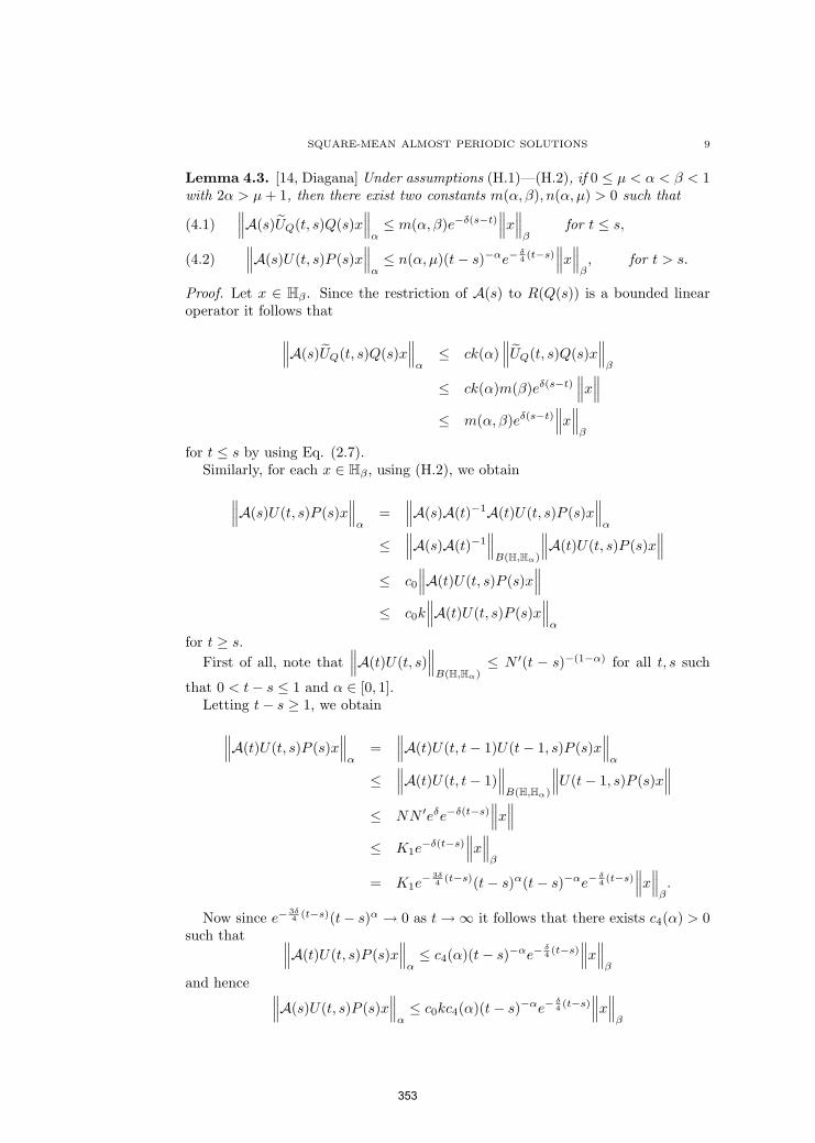
SQUARE-MEAN ALMOST PERIODIC SOLUTIONS 9
Lemma 4.3. [14, Diagana] Under assumptions (H.1)—(H.2), if 0 ≤ µ < α < β < 1with 2α > µ + 1, then there exist two constants m(α, β), n(α, µ) > 0 such that∥∥∥A(s)UQ(t, s)Q(s)x
∥∥∥α≤ m(α, β)e−δ(s−t)
∥∥∥x∥∥∥
βfor t ≤ s,(4.1) ∥∥∥A(s)U(t, s)P (s)x
∥∥∥α≤ n(α, µ)(t− s)−αe−
δ4 (t−s)
∥∥∥x∥∥∥
β, for t > s.(4.2)
Proof. Let x ∈ Hβ . Since the restriction of A(s) to R(Q(s)) is a bounded linearoperator it follows that∥∥∥A(s)UQ(t, s)Q(s)x
∥∥∥α
≤ ck(α)∥∥∥UQ(t, s)Q(s)x
∥∥∥β
≤ ck(α)m(β)eδ(s−t)∥∥∥x
∥∥∥≤ m(α, β)eδ(s−t)
∥∥∥x∥∥∥
β
for t ≤ s by using Eq. (2.7).Similarly, for each x ∈ Hβ , using (H.2), we obtain∥∥∥A(s)U(t, s)P (s)x
∥∥∥α
=∥∥∥A(s)A(t)−1A(t)U(t, s)P (s)x
∥∥∥α
≤∥∥∥A(s)A(t)−1
∥∥∥B(H,Hα)
∥∥∥A(t)U(t, s)P (s)x∥∥∥
≤ c0
∥∥∥A(t)U(t, s)P (s)x∥∥∥
≤ c0k∥∥∥A(t)U(t, s)P (s)x
∥∥∥α
for t ≥ s.First of all, note that
∥∥∥A(t)U(t, s)∥∥∥
B(H,Hα)≤ N ′(t − s)−(1−α) for all t, s such
that 0 < t− s ≤ 1 and α ∈ [0, 1].Letting t− s ≥ 1, we obtain∥∥∥A(t)U(t, s)P (s)x
∥∥∥α
=∥∥∥A(t)U(t, t− 1)U(t− 1, s)P (s)x
∥∥∥α
≤∥∥∥A(t)U(t, t− 1)
∥∥∥B(H,Hα)
∥∥∥U(t− 1, s)P (s)x∥∥∥
≤ NN ′eδe−δ(t−s)∥∥∥x
∥∥∥≤ K1e
−δ(t−s)∥∥∥x
∥∥∥β
= K1e− 3δ
4 (t−s)(t− s)α(t− s)−αe−δ4 (t−s)
∥∥∥x∥∥∥
β.
Now since e−3δ4 (t−s)(t− s)α → 0 as t →∞ it follows that there exists c4(α) > 0
such that ∥∥∥A(t)U(t, s)P (s)x∥∥∥
α≤ c4(α)(t− s)−αe−
δ4 (t−s)
∥∥∥x∥∥∥
β
and hence ∥∥∥A(s)U(t, s)P (s)x∥∥∥
α≤ c0kc4(α)(t− s)−αe−
δ4 (t−s)
∥∥∥x∥∥∥
β
353
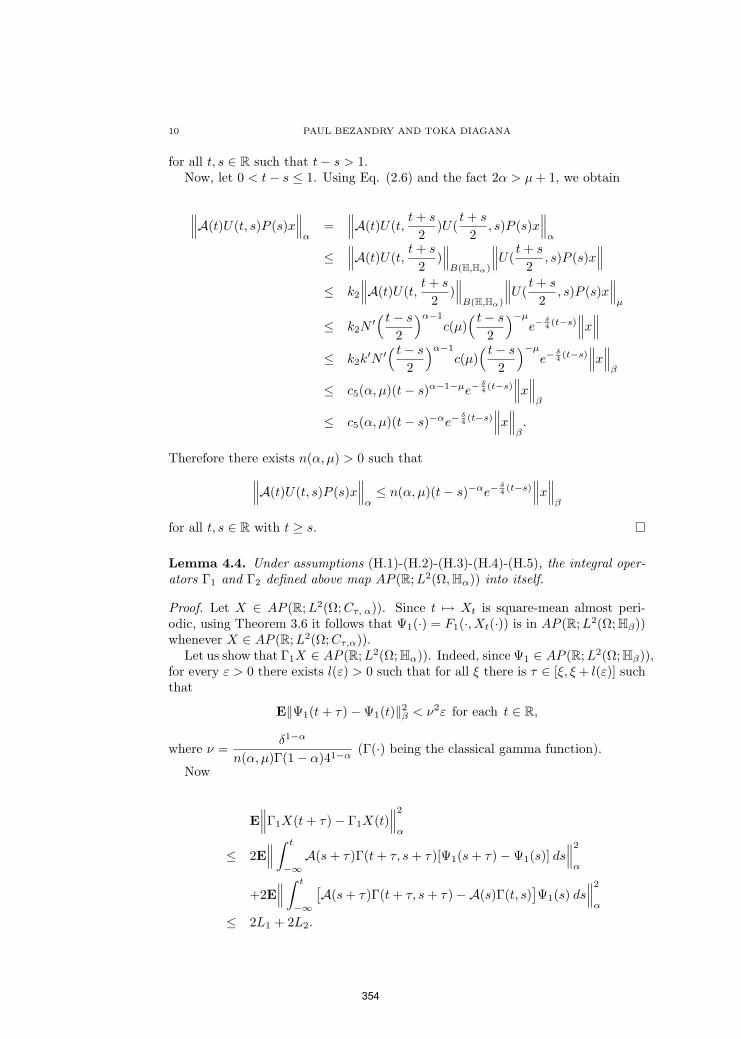
10 PAUL BEZANDRY AND TOKA DIAGANA
for all t, s ∈ R such that t− s > 1.Now, let 0 < t− s ≤ 1. Using Eq. (2.6) and the fact 2α > µ + 1, we obtain
∥∥∥A(t)U(t, s)P (s)x∥∥∥
α=
∥∥∥A(t)U(t,t + s
2)U(
t + s
2, s)P (s)x
∥∥∥α
≤∥∥∥A(t)U(t,
t + s
2)∥∥∥
B(H,Hα)
∥∥∥U(t + s
2, s)P (s)x
∥∥∥≤ k2
∥∥∥A(t)U(t,t + s
2)∥∥∥
B(H,Hα)
∥∥∥U(t + s
2, s)P (s)x
∥∥∥µ
≤ k2N′( t− s
2
)α−1
c(µ)( t− s
2
)−µ
e−δ4 (t−s)
∥∥∥x∥∥∥
≤ k2k′N ′
( t− s
2
)α−1
c(µ)( t− s
2
)−µ
e−δ4 (t−s)
∥∥∥x∥∥∥
β
≤ c5(α, µ)(t− s)α−1−µe−δ4 (t−s)
∥∥∥x∥∥∥
β
≤ c5(α, µ)(t− s)−αe−δ4 (t−s)
∥∥∥x∥∥∥
β.
Therefore there exists n(α, µ) > 0 such that∥∥∥A(t)U(t, s)P (s)x∥∥∥
α≤ n(α, µ)(t− s)−αe−
δ4 (t−s)
∥∥∥x∥∥∥
β
for all t, s ∈ R with t ≥ s.
Lemma 4.4. Under assumptions (H.1)-(H.2)-(H.3)-(H.4)-(H.5), the integral oper-ators Γ1 and Γ2 defined above map AP (R; L2(Ω, Hα)) into itself.
Proof. Let X ∈ AP (R;L2(Ω;Cτ, α)). Since t 7→ Xt is square-mean almost peri-odic, using Theorem 3.6 it follows that Ψ1(·) = F1(·, Xt(·)) is in AP (R; L2(Ω; Hβ))whenever X ∈ AP (R;L2(Ω;Cτ,α)).
Let us show that Γ1X ∈ AP (R; L2(Ω; Hα)). Indeed, since Ψ1 ∈ AP (R; L2(Ω; Hβ)),for every ε > 0 there exists l(ε) > 0 such that for all ξ there is τ ∈ [ξ, ξ + l(ε)] suchthat
E‖Ψ1(t + τ)−Ψ1(t)‖2β < ν2ε for each t ∈ R,
where ν =δ1−α
n(α, µ)Γ(1− α)41−α(Γ(·) being the classical gamma function).
Now
E∥∥∥Γ1X(t + τ)− Γ1X(t)
∥∥∥2
α
≤ 2E∥∥∥∫ t
−∞A(s + τ)Γ(t + τ, s + τ)[Ψ1(s + τ)−Ψ1(s)] ds
∥∥∥2
α
+2E∥∥∥∫ t
−∞
[A(s + τ)Γ(t + τ, s + τ)−A(s)Γ(t, s)
]Ψ1(s) ds
∥∥∥2
α
≤ 2L1 + 2L2.
354

SQUARE-MEAN ALMOST PERIODIC SOLUTIONS 11
Using the estimate in Eq. (4.2) yields
L1 ≤ E ∫ t
−∞
∥∥∥A(s + τ)Γ(t + τ, s + τ)[Ψ1(s + τ)−Ψ1(s)]∥∥∥ ds
2
≤ n(α, µ)2 E ∫ t
−∞(t− s)−α e−
δ4 (t−s)
∥∥∥Ψ1(s + τ)−Ψ1(s)∥∥∥ ds
2
≤ n(α, µ)2( ∫ t
−∞(t− s)−αe−
δ4 (t−s) ds
)2
supt
E∥∥∥Ψ1(t + τ)−Ψ1(t)
∥∥∥2
β
≤ n(α, µ)2(
Γ(1− α)41−α
δ1−α
)2
supt
E∥∥∥Ψ1(t + τ)−Ψ1(t)
∥∥∥2
β< ε.
Similarly, using assumption (H.3), it follows that
L2 ≤ E ∫ t
−∞
∥∥∥A(s + τ)Γ(t + τ, s + τ)−A(s)Γ(t, s)∥∥∥ ∥∥∥Ψ1(s)
∥∥∥α
ds
2
≤ ε2
∫ t
−∞γ(t− s) ds
∫ t
−∞γ(t− s)E
∥∥∥Ψ1(s)∥∥∥2
αds
≤ ε2
( ∫ t
−∞γ(t− s) ds
)2
supt
E∥∥∥Ψ1(s)
∥∥∥2
α= ε2k(α)
∥∥γ∥∥2
L1 KΨ1 .
Therefore,
E∥∥∥Γ1X(t + τ)− Γ1X(t)
∥∥∥2
α≤
(2 + 2k(α)
∥∥γ∥∥2
L1 KΨ1ε
)ε,
for each t ∈ R, and hence Γ1X ∈ AP (R; L2(Ω; Hα)).The proof for Γ2X(·) is omitted as it follows along the same line as that of
Γ1X.
Lemma 4.5. Under assumptions (H.1)-(H.2)-(H.3)-(H.4)-(H.5), the integral oper-ators Γ3 and Γ4 defined above map AP (R; L2(Ω; Hα)) into itself.
Proof. The proof for the square-mean almost periodicity of Γ4X is similar to thatof Γ3X and hence will be omitted. Note, however, that for Γ4X, we make use ofEq. (2.7 ) rather than Eq. (2.6 ).
Let X ∈ AP (R;L2(Ω, Cτ,α)). Clearly, Xt ∈ AP (R; L2(Ω, Cτ,α)). Setting Ψ2(t) =F2(t, Xt) and using Theorem 3.7 it follows that Ψ2 ∈ AP (R;L2(Ω, H)).
We now show that Γ3X ∈ AP (R; L2(Ω, Hα)). Indeed, since Ψ2 ∈ AP (R; L2(Ω, H)),for every ε > 0 there exists l(ε) > 0 such that for all ξ there is τ ∈ [ξ, ξ + l(ε)] with
E∥∥∥Ψ2(t + τ)−Ψ2(t)
∥∥∥2
< κ2 · ε for each t ∈ R,
where κ =δ1−α
c(α)21−αΓ(1− α)(Γ(·) being the classical gamma function).
355

12 PAUL BEZANDRY AND TOKA DIAGANA
Now
E∥∥∥(Γ3X)(t + τ)− (Γ3X)(t)
∥∥∥2
α
= E∥∥∥∥∫ t
−∞Γ(t + τ, s + τ)Ψ2(s + τ) ds−
∫ t
−∞Γ(t, s)Ψ2(s) ds
∥∥∥∥2
α
≤ 3E∥∥∥∥∫ ∞
0
Γ(t + τ, t− s + τ)[Ψ2(t− s + τ)−Ψ2(t− s)] ds
∥∥∥∥2
α
+3E∥∥∥∥∫ ∞
ε
[Γ(t + τ, t− s + τ)− Γ(t, t− s)
]Ψ2(t− s) ds
∥∥∥∥2
α
+3E∥∥∥∥∫ ε
0
[Γ(t + τ, t− s + τ)− Γ(t, t− s)
]Ψ2(t− s) ds
∥∥∥∥2
α
≤ 3L′1 + 3L′2 + 3L′3.
Using Eq. (2.6), it follows that
L′1 ≤ E ∫ ∞
0
∥∥∥Γ(t + τ, t− s + τ)[Ψ2(t− s + τ)−Ψ2(t− s)]∥∥∥
αds
2
≤ c(α)2E ∫ ∞
0
s−αe−δ2 s
∥∥∥Ψ2(t− s + τ)−Ψ2(t− s)∥∥∥ ds
2
≤ c(α)2( ∫ ∞
0
s−αe−δ2 s ds
)2
supt
E∥∥∥Ψ2(t + τ)−Ψ2(t)
∥∥∥≤ c(α)2
(Γ(1− α)21−α
δ1−α
)2
supt
E∥∥∥Ψ2(t + τ)−Ψ2(t)
∥∥∥ ≤ ε .
For L′2, we use [25, Proposition 4.4] to obtain
L′2 ≤ E ∫ ∞
ε
∥∥∥[Γ(t + τ, t− s + τ)− Γ(t, t− s)
]Ψ2(t− s)
∥∥∥α
ds
2
≤ 4δ2
ε2 supt∈R
E∥∥∥Ψ2(t)
∥∥∥2
.
The evaluation of the last term is straightforward. We obtain:
L′3 ≤ E ∫ ε
0
∥∥∥[Γ(t + τ, t− s + τ)− Γ(t, t− s)
]Ψ2(t− s)
∥∥∥α
ds
2
≤ 4 M2 ε2 supt∈R
E∥∥∥Ψ2(t)
∥∥∥2
.
Combining these evaluations, we conclude that Γ3X ∈ AP (R; L2(Ω; Hα)).
Lemma 4.6. Under assumptions (H.1)-(H.2)-(H.3)-(H.4)-(H.5), the integral oper-ators Γ5 and Γ6 defined above map AP (R; L2(Ω; Hα)) into itself.
Proof. Let X ∈ AP (R; L2(Ω;Cτ,α)). Setting Ψ3(t) = F3(t, Xt) and using Theorem3.7 it follows that Ψ3 ∈ AP (R; L2(Ω; H)). We claim that Γ5X ∈ AP (R; L2(Ω; Hα)).Indeed, since Ψ3 ∈ AP (R;L2(Ω; H)), for every ε > 0 there exists l(ε) > 0 such thatfor all ξ there is τ ∈ [ξ, ξ + l(ε)] with
E‖Ψ3(t + τ)−Ψ3(t)‖2 < ζ · ε for each t ∈ R,(4.3)
356
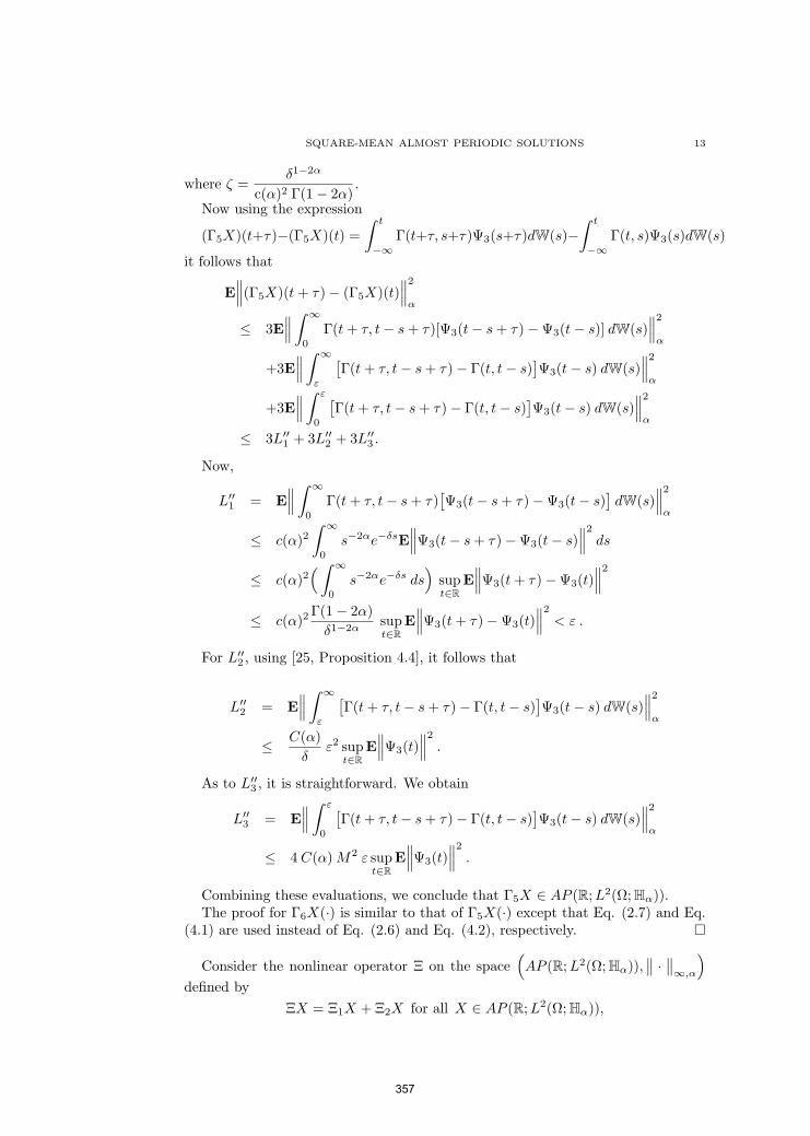
SQUARE-MEAN ALMOST PERIODIC SOLUTIONS 13
where ζ =δ1−2α
c(α)2 Γ(1− 2α).
Now using the expression
(Γ5X)(t+τ)−(Γ5X)(t) =∫ t
−∞Γ(t+τ, s+τ)Ψ3(s+τ)dW(s)−
∫ t
−∞Γ(t, s)Ψ3(s)dW(s)
it follows that
E∥∥∥(Γ5X)(t + τ)− (Γ5X)(t)
∥∥∥2
α
≤ 3E∥∥∥∫ ∞
0
Γ(t + τ, t− s + τ)[Ψ3(t− s + τ)−Ψ3(t− s)] dW(s)∥∥∥2
α
+3E∥∥∥∫ ∞
ε
[Γ(t + τ, t− s + τ)− Γ(t, t− s)
]Ψ3(t− s) dW(s)
∥∥∥2
α
+3E∥∥∥∫ ε
0
[Γ(t + τ, t− s + τ)− Γ(t, t− s)
]Ψ3(t− s) dW(s)
∥∥∥2
α
≤ 3L′′1 + 3L′′2 + 3L′′3 .
Now,
L′′1 = E∥∥∥∫ ∞
0
Γ(t + τ, t− s + τ)[Ψ3(t− s + τ)−Ψ3(t− s)
]dW(s)
∥∥∥2
α
≤ c(α)2∫ ∞
0
s−2αe−δsE∥∥∥Ψ3(t− s + τ)−Ψ3(t− s)
∥∥∥2
ds
≤ c(α)2( ∫ ∞
0
s−2αe−δs ds)
supt∈R
E∥∥∥Ψ3(t + τ)−Ψ3(t)
∥∥∥2
≤ c(α)2Γ(1− 2α)
δ1−2αsupt∈R
E∥∥∥Ψ3(t + τ)−Ψ3(t)
∥∥∥2
< ε .
For L′′2 , using [25, Proposition 4.4], it follows that
L′′2 = E∥∥∥∫ ∞
ε
[Γ(t + τ, t− s + τ)− Γ(t, t− s)
]Ψ3(t− s) dW(s)
∥∥∥2
α
≤ C(α)δ
ε2 supt∈R
E∥∥∥Ψ3(t)
∥∥∥2
.
As to L′′3 , it is straightforward. We obtain
L′′3 = E∥∥∥∫ ε
0
[Γ(t + τ, t− s + τ)− Γ(t, t− s)
]Ψ3(t− s) dW(s)
∥∥∥2
α
≤ 4 C(α) M2 ε supt∈R
E∥∥∥Ψ3(t)
∥∥∥2
.
Combining these evaluations, we conclude that Γ5X ∈ AP (R; L2(Ω; Hα)).The proof for Γ6X(·) is similar to that of Γ5X(·) except that Eq. (2.7) and Eq.
(4.1) are used instead of Eq. (2.6) and Eq. (4.2), respectively.
Consider the nonlinear operator Ξ on the space(AP (R;L2(Ω; Hα)),
∥∥ · ∥∥∞,α
)defined by
ΞX = Ξ1X + Ξ2X for all X ∈ AP (R; L2(Ω; Hα)),
357

14 PAUL BEZANDRY AND TOKA DIAGANA
where
(Ξ1X)(t) = −F1(t, Xt)−∫ t
−∞A(s)Γ(t, s) F1(s,Xs) ds +
∫ ∞
t
A(s)Γ(t, s) F1(s,Xs)) ds
(Ξ2X)(t) =∫ t
−∞Γ(t, s) F2(s,Xs)) ds−
∫ ∞
t
Γ(t, s) F2(s,Xs) ds
+∫ t
−∞Γ(t, s) F3(s,Xs) dW(s)−
∫ ∞
t
Γ(t, s) F3(s,Xs) dW(s).
In view of Lemma 4.4, Lemma 4.5, and Lemma 4.6, it follows that Ξ mapsAP (R;L2(Ω; Hα)) into itself. In order to apply Krasnoselskii’s fixed point theorem,we need to construct two mappings: a contraction map and a compact map.
Lemma 4.7. The operator Ξ1 is a contraction provided K(α, β, δ, µ, K1) < 1.
Proof. Let X, Y ∈ AP (R; L2(Ω; Hα)). Using (H.1)-(H4), we obtain
E∥∥∥F1(t, Xt)− F1(t, Yt)
∥∥∥2
α≤ k(α)K1E
∥∥∥Xt − Yt
∥∥∥2
τ,α
≤ k(α) ·K1
∥∥∥X − Y∥∥∥2
∞,α,
which yields
∥∥∥F1(·, X·)− F1(·, Y·)∥∥∥∞,α
≤ k′(α) ·K ′1
∥∥∥X − Y∥∥∥∞,α
.
Now for Γ1 and Γ2, we have the following evaluations
E∥∥∥(Γ1X)(t)− (Γ1Y )(t)
∥∥∥2
α
≤ E( ∫ t
−∞
∥∥∥A(s)Γ(t, s)[F1(s,Xs)− F1(s, Ys)]∥∥∥
αds
)2
≤ n(α, µ)2( ∫ t
−∞(t− s)−αe−
δ4 (t−s) ds
)×
×( ∫ t
−∞(t− s)−αe−
δ4 (t−s)E
∥∥∥F1(s,Xs)− F1(s, Ys)∥∥∥2
βds
)≤ n(α, µ)2 K1
( ∫ t
−∞(t− s)−αe−
δ4 (t−s) ds
)2 ∥∥∥X − Y∥∥∥2
∞,α,
and hence
∥∥∥Γ1X − Γ1Y∥∥∥∞,α
≤ n(α, µ) ·K ′1
41−αΓ(1− α))δ1−α
∥∥∥X − Y∥∥∥∞,α
.
358

SQUARE-MEAN ALMOST PERIODIC SOLUTIONS 15
Similarly,
E∥∥∥(Γ2X)(t)− (Γ2Y )(t)
∥∥∥2
α
≤ E( ∫ ∞
t
∥∥∥A(s)Γ(t, s)[F1(s,Xs)− F1(s, Ys)]∥∥∥
αds
)2
≤ m(α, β)2( ∫ ∞
t
e−δ(s−t) ds)×
×( ∫ ∞
t
e−δ(s−t)E‖F1(s,Xs)− F1(s, Ys)‖2β ds
)≤ m(α, β)2 k(α) K1
( ∫ ∞
t
e−δ(s−t) ds)2 ∥∥∥X − Y
∥∥∥2
∞,α,
and hence, ∥∥∥Γ2X − Γ2Y∥∥∥∞,α
≤ m(α, β) · k′(α) ·K ′1
δ
∥∥∥X − Y∥∥∥∞,α
.
Lemma 4.8. The nonlinear operator Ξ2 is continuous. Moreover, its image iscontained in a compact set.
Proof. Let us consider the set V =X ∈ AP (R;L2(Ω, Hα)) : ‖X‖2
∞,α ≤ R′
forsome fixed R′ > 0. For the continuity, let Xn ∈ AP (R;L2(Ω, Hα)) be a sequencewhich converges to some X ∈ AP (R;L2(Ω, Hα)), that is, ‖Xn − X‖∞,α → 0 asn →∞. It follows from the estimates in Lemma 2.3 that
E∥∥∥∫ t
−∞Γ(t, s)[F2(s,Xn
s )− F2(s,Xs)] ds∥∥∥2
α
≤ E
[ ∫ t
−∞c(α)(t− s)−αe−
δ2 (t−s)
∥∥∥F2(s,Xns )− F2(s,Xs)
∥∥∥ ds
]2
.
Now, using the continuity of F2 and the Lebesgue Dominated Convergence Theoremwe obtain that
E∥∥∥∫ t
−∞Γ(t, s)[F2(s,Xn
s )− F2(s,Xs)] ds∥∥∥2
α→ 0 as n →∞ .
By similar arguments, we can also show that
E∥∥∥∫ ∞
t
Γ(t, s)[F2(s,Xns )− F2(s,Xs)] ds
∥∥∥2
α→ 0 as n →∞ .
For the term containing the Brownian motion W, we use the estimates (4.1) and(4.2) to obtain
E∥∥∥∫ t
−∞Γ(t, s)[F3(s,Xn
s )− F3(s,Xs)] dW(s)∥∥∥2
α
≤ C(α)2∫ t
−∞(t− s)−2αe−δ (t−s)E
∥∥∥F3(s,Xns )− F3(s,Xs)
∥∥∥2
ds .
359

16 PAUL BEZANDRY AND TOKA DIAGANA
Now, using the continuity of F3 and the Lebesgue Dominated Convergence Theoremwe obtain that
E∥∥∥∫ t
−∞Γ(t, s)[F3(s,Xn
s )− F3(s,Xs)] dW(s)∥∥∥2
α→ 0 as n →∞ .
By similar arguments, we can also show that
E∥∥∥∫ ∞
t
Γ(t, s)[F3(s,Xns )− F3(s,Xs)] dW(s)
∥∥∥2
α→ 0 as n →∞ .
Therefore, ∥∥∥Ξ2Xn − Ξ2X
∥∥∥∞,α
→ 0 as n →∞.
We now show that Ξ2 maps V into a compact set; in particular, we show thatΞ2(V ) is an equicontinuous set. Indeed, let ε > 0, t1 < t2, and X ∈ V be arbitrary.
Now
E∥∥∥(Ξ2X)(t2)− (Ξ2X)(t1)
∥∥∥2
α
≤ 4E∥∥∥(Γ3X)(t2)− (Γ3X)(t1)
∥∥∥2
α+ 4E
∥∥∥(Γ4X)(t2)− (Γ4X)(t1)∥∥∥2
α
+4E∥∥∥(Γ5X)(t2)− (Γ5X)(t1)
∥∥∥2
α+ 4E
∥∥∥(Γ6X)(t2)− (Γ6X)(t1)∥∥∥2
α.
We have
E∥∥∥(Γ3X)(t2)− (Γ3X)(t1)
∥∥∥2
α
≤ 2E∥∥∥∫ t2
t1
U(t2, s)P (s) Ψ2(s) ds∥∥∥2
α+ 2E
∥∥∥∫ t1
−∞[U(t2, s)− U(t1, s)]P (s) Ψ2(s) ds
∥∥∥2
α
= 2E∥∥∥∫ t2
t1
U(t2, s)P (s) Ψ2(s) ds∥∥∥2
α+ 2E
∥∥∥∫ t1
−∞
( ∫ t2
t1
∂U(τ, s)∂τ
dτ)P (s) Ψ2(s) ds
∥∥∥2
α
= 2E∥∥∥∫ t2
t1
U(t2, s)P (s) Ψ2(s) ds∥∥∥2
α+ 2E
∥∥∥∫ t1
−∞
( ∫ t2
t1
A(τ)U(τ, s)P (s) Ψ2(s) dτ)
ds∥∥∥2
α
= 2N1 + 2N2.
Clearly,
N1 ≤ E∫ t2
t1
∥∥∥U(t2, s)P (s) Ψ2(s)∥∥∥
αds
2
≤ c(α)2E∫ t2
t1
(t2 − s)−αe−δ2 (t2−s)
∥∥∥Ψ2(s)∥∥∥ ds
2
.
Similarly,
N2 ≤ E∫ t1
−∞
( ∫ t2
t1
∥∥∥A(τ)U(τ, s)P (s) Ψ2(s)∥∥∥
αdτ
)ds
2
≤ c20 E
∫ t1
−∞
( ∫ t2
t1
∥∥∥A(s)U(τ, s)P (s) Ψ2(s)∥∥∥
αdτ
)ds
2
≤ c20 n(α, µ)2 E
∫ t1
−∞
( ∫ t2
t1
(τ − s)−αe−δ2 (τ−s)
∥∥∥Ψ2(s)∥∥∥
βdτ
)ds
2
.
360

SQUARE-MEAN ALMOST PERIODIC SOLUTIONS 17
Therefore,
E∥∥∥(Γ3X)(t2)− (Γ3X)(t1)
∥∥∥2
α
≤ 2 c(α)2E∫ t2
t1
(t2 − s)−αe−δ2 (t2−s)
∥∥∥Ψ2(s)∥∥∥ ds
2
+2 c20 n(α, µ)2 E
∫ t1
−∞
( ∫ t2
t1
(τ − s)−αe−δ2 (τ−s)
∥∥∥Ψ2(s)∥∥∥
βdτ
)ds
2
≤ K(α, δ, µ) (t2 − t1)2 supt∈R
E∥∥∥Ψ2(t)
∥∥∥2
,
where K(α, δ, µ) is a positive constant.Similar computations show that
E∥∥∥(Γ4X)(t2)− (Γ4X)(t1)
∥∥∥2
α
≤ 2 c(α)2E∫ t2
t1
e− δ(s−t1)∥∥∥Ψ2(s)
∥∥∥ ds2
+2 c20 m(α, β)2 E
∫ ∞
t2
( ∫ t2
t1
e− δ(s−τ)∥∥∥Ψ2(s)
∥∥∥β
dτ)
ds2
≤ K(α, δ, β) (t2 − t1)2 supt∈R
E∥∥∥Ψ2(t)
∥∥∥2
,
where K(α, δ, β) is a positive constant.Let us now evaluate Γ5X. We have
E∥∥∥(Γ5X)(t2)− (Γ5X)(t1)
∥∥∥2
α
≤ 2E∥∥∥∫ t2
t1
U(t2, s)P (s) Ψ3(s) dW(s)∥∥∥2
α
+2E∥∥∥∫ t1
−∞[U(t2, s)− U(t1, s)]P (s) Ψ3(s) dW(s)
∥∥∥2
α
= 2N ′1 + 2N ′
2.
Let us start with the first term. By Ito isometry identity, we have
N ′1 ≤ c(α)2
∫ t2
t1
(t2 − s)−2αe− δ(t2−s)E∥∥∥Ψ3(s)
∥∥∥2
ds
≤ c(α)2( ∫ t2
t1
(t2 − s)−2αe− δ (t2−s) ds)
sups∈R
E∥∥∥Ψ3(s)
∥∥∥2
.
361
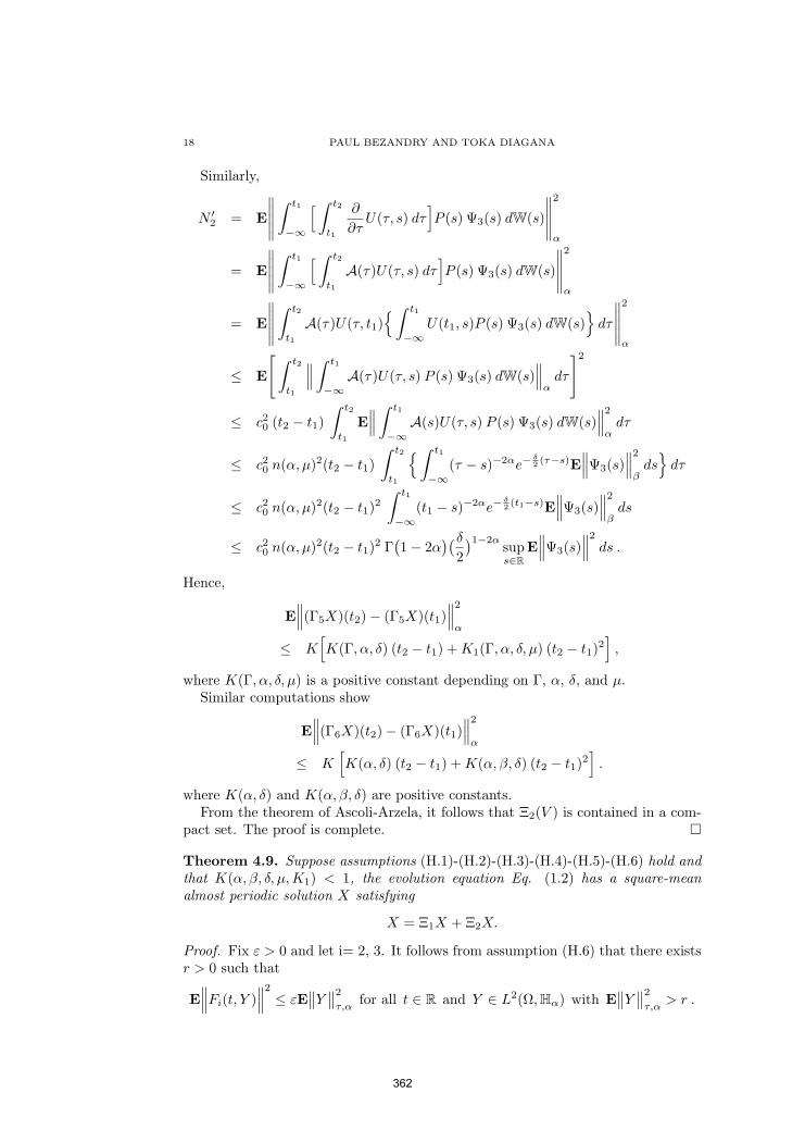
18 PAUL BEZANDRY AND TOKA DIAGANA
Similarly,
N ′2 = E
∥∥∥∥∥∫ t1
−∞
[ ∫ t2
t1
∂
∂τU(τ, s) dτ
]P (s) Ψ3(s) dW(s)
∥∥∥∥∥2
α
= E
∥∥∥∥∥∫ t1
−∞
[ ∫ t2
t1
A(τ)U(τ, s) dτ]P (s) Ψ3(s) dW(s)
∥∥∥∥∥2
α
= E
∥∥∥∥∥∫ t2
t1
A(τ)U(τ, t1)∫ t1
−∞U(t1, s)P (s) Ψ3(s) dW(s)
dτ
∥∥∥∥∥2
α
≤ E
[ ∫ t2
t1
∥∥∥∫ t1
−∞A(τ)U(τ, s) P (s) Ψ3(s) dW(s)
∥∥∥α
dτ
]2
≤ c20 (t2 − t1)
∫ t2
t1
E∥∥∥∫ t1
−∞A(s)U(τ, s) P (s) Ψ3(s) dW(s)
∥∥∥2
αdτ
≤ c20 n(α, µ)2(t2 − t1)
∫ t2
t1
∫ t1
−∞(τ − s)−2αe−
δ2 (τ−s)E
∥∥∥Ψ3(s)∥∥∥2
βds
dτ
≤ c20 n(α, µ)2(t2 − t1)2
∫ t1
−∞(t1 − s)−2αe−
δ2 (t1−s)E
∥∥∥Ψ3(s)∥∥∥2
βds
≤ c20 n(α, µ)2(t2 − t1)2 Γ
(1− 2α
)(δ
2)1−2α sup
s∈RE
∥∥∥Ψ3(s)∥∥∥2
ds .
Hence,
E∥∥∥(Γ5X)(t2)− (Γ5X)(t1)
∥∥∥2
α
≤ K[K(Γ, α, δ) (t2 − t1) + K1(Γ, α, δ, µ) (t2 − t1)2
],
where K(Γ, α, δ, µ) is a positive constant depending on Γ, α, δ, and µ.Similar computations show
E∥∥∥(Γ6X)(t2)− (Γ6X)(t1)
∥∥∥2
α
≤ K[K(α, δ) (t2 − t1) + K(α, β, δ) (t2 − t1)2
].
where K(α, δ) and K(α, β, δ) are positive constants.From the theorem of Ascoli-Arzela, it follows that Ξ2(V ) is contained in a com-
pact set. The proof is complete.
Theorem 4.9. Suppose assumptions (H.1)-(H.2)-(H.3)-(H.4)-(H.5)-(H.6) hold andthat K(α, β, δ, µ, K1) < 1, the evolution equation Eq. (1.2) has a square-meanalmost periodic solution X satisfying
X = Ξ1X + Ξ2X.
Proof. Fix ε > 0 and let i= 2, 3. It follows from assumption (H.6) that there existsr > 0 such that
E∥∥∥Fi(t, Y )
∥∥∥2
≤ εE∥∥Y
∥∥2
τ,αfor all t ∈ R and Y ∈ L2(Ω, Hα) with E
∥∥Y∥∥2
τ,α> r .
362
SQUARE-MEAN ALMOST PERIODIC SOLUTIONS 19
Setting
Mi = supE
∥∥∥Fi(t, Y )∥∥∥2
: t ∈ R, E∥∥Y
∥∥2
τ,α≤ r
.
Therefore,
E∥∥∥Fi(t, Y )
∥∥∥2
≤ Mi + εE∥∥Y
∥∥2
τ,αfor all (t, Y ) ∈ R× L2(Ω, Cτ,α) .(4.4)
Also, using Lemma 2.3 , Eq. (4.1), Eq. (4.2), Eq. (4.4), and assumption (H.4) wecan show that
E∥∥∥(Ξ1X)(t) + (Ξ2Y )(t)
∥∥∥2
α
≤ 12[1 + n(α, µ)2
(Γ(1− α) 21−α
δ1−α
)2
+(m(α, β)
δ
)2](K1
∥∥X∥∥∞,α
+ supt∈R
∥∥∥F1(t, 0)∥∥∥2)
+ 8c(α)2[[(Γ(1− α) 21−α
δ1−α
)2
+(m(α)
δ
)2](M2 + ε
∥∥Y∥∥∞,α
)+
[K(α)
Γ(1− 2α)δ1−2α
+K(α, β)
2δ
] (M3 + ε
∥∥Y∥∥∞,α
)]
= c1(α, β, δ, µ, Γ)(K1
∥∥X∥∥∞,α
+ supt∈R
∥∥∥F1(t, 0)∥∥∥2)
+ c2(α, β, δ, Γ)(M2 + ε
∥∥Y∥∥∞,α
)+ c3(α, β, δ, Γ)
(M3 + ε
∥∥Y∥∥∞,α
).
Now, for ε, K1 small enough, choose R such that
c1(α, β, δ, µ, Γ)(K1R+a
)+c2(α, β, δ, Γ)
(M2+εR
)+c3(α, β, δ, Γ)
(M3+εR
)≤ R
where a = supt∈R
∥∥∥F1(t, 0)∥∥∥2
, c1(α, β, δ, µ, Γ) and ci(α, β, δ, Γ) (i = 2, 3) are constants
depending on α, β , δ, and the classical gamma function Γ(·).
Let W =
Z ∈ AP (R;L2(Ω; Hα) :
∥∥Z∥∥∞,α
≤ R
. For X, Y ∈ W , we have
E∥∥∥(Ξ1X)(t) + (Ξ2Y )(t)
∥∥∥2
α≤ R .
Thus (Ξ1X)(t) + (Ξ2Y )(t) ∈ W . In view of Lemma 4.4, Lemma 4.5, Lemma 4.6,Lemma 4.7, and Lemma 4.8, the proof can be completed by using the Krasnoselskii’sfixed point theorem (Theorem 4.2).
5. Example
Throughout the rest of this paper, we suppose 0 < α < 0.5 < β < 1.
Example 5.1. Fix T > 0. Let H = L2[0, π] equipped with its natural topology.Here, for µ ∈ (0, 1), we take Hµ =
(L2[0, π], H1
0[0, π] ∩H2[0, π])
µ,∞equipped with
its µ-norm ‖ · ‖µ.
363
20 PAUL BEZANDRY AND TOKA DIAGANA
To illustrate our main result, we study the existence of square-mean almostperiodic solutions to the one-dimensional stochastic heat equation with finite delaygiven by(5.1)
∂
[Φ + F1(t,Φt)
]=
[∂2Φ∂x2
+ a(t, x)Φ + F2(t,Φt)
]∂t + F3(t,Φt)dW(t), R× [0, π]
Φ(t, 0) = Φ(t, π) = 0, t ∈ R
where a : R × [0, π] 7→ R is T -periodic in t ∈ R uniformly in x ∈ [0, π], andF1 : R×L2(Ω; Bα) 7→ L2(Ω, Hβ) and Fi(i = 2, 3) : R×L2(Ω,Bα) → L2(Ω, L2[0, π])are square-mean almost periodic processes.
Define the corresponding linear operator A(t) on L2(Ω, L2[0, π]) as follows:
A(t)Φ =∂2Φ∂x2
+ a(t, x)Φ for all Φ ∈ D(A(t)) = L2(Ω, H10[0, π] ∩H2[0, π]),
where a : R × [0, π] 7→ R, in addition of being T -periodic satisfies: there existδ0 ∈ (0, 1) such that
a(t, x) ≤ δ0
for all t ∈ R and x ∈ [0, π].Clearly, A(t+T ) = A(t) for all t ∈ R. Moreover, it is then easy to check that the
evolution family U(t, s) associated with A(t) is exponentially stable, which yieldsdichotomy with dichotomy projections P (t) = I and Q(t) = 0. Indeed,
U(t, s) = T (t− s)e
∫ t
s
a(τ, x)dτfor all t ≥ s,
where T (t) is the analytic semigroup associated with the second-order differentialoperator
AΦ =∂2Φ∂x2
with D(A) = L2(Ω, H10[0, π] ∩H2[0, π]).
Now
‖U(t, s)Φ‖ ≤ e−(1−δ0)(t−s)‖Φ‖, t ≥ s.
Moreover, U(t + T, s + T ) = U(t, s) for all t ≥ s. Now since Q(t) = 0, it followsthat Γ(t, s) = U(t, s) and hence
A(t + T )Γ(t + T, s + T ) = A(t)Γ(t, s).
We have
Theorem 5.2. Under previous assumptions, then the heat equation Eq. (5.1) hasa solution Φ ∈ AP (R, L2([0, π], Hα)).
Acknowledgment. The authors express their thanks to the referees for carefulreading of the manuscript and insightful comments, which greatly helped to improvethe paper.
364

SQUARE-MEAN ALMOST PERIODIC SOLUTIONS 21
References
1. P. Acquistapace, Evolution operators and strong solutions of abstract linear parabolic equa-
tions, Differential Integral Equations 1 (1988), 433–457.
2. P. Acquistapace, F. Flandoli, B. Terreni, Initial boundary value problems and optimal control
for nonautonomous parabolic systems. SIAM J. Control Optim. 29 (1991), 89–118.
3. P. Acquistapace, B. Terreni, A unified approach to abstract linear nonautonomous parabolic
equations, Rend. Sem. Mat. Univ. Padova 78 (1987), 47–107.
4. H. Amann, Linear and Quasilinear Parabolic Problems, Birkhauser, Berlin 1995.
5. B. Amir and L. Maniar, Existence and some asymptotic behaviors of solutions to semilinear
Cauchy problems with non dense domain via extrapolation spaces, Rend. Circ. Mat. Palermo
(2000) 481-496.
6. L. Arnold and C. Tudor, Stationary and Almost Periodic Solutions of Almost Periodic Affine
Stochastic Differential Equations, Stochastics and Stochastic Reports 64 (1998), 177-193.
7. M. Baroun, S. Boulite, T. Diagana, and L. Maniar, Almost periodic solutions to some semi-
linear non-autonomous thermoelastic plate equations. J. Math. Anal. Appl. 349(2009), no. 1,
74–84.
8. P. Bezandry and T. Diagana; Existence of Almost Periodic Solutions to Some Stochastic
Differential Equations. Applicable Anal. 86 (2007), no. 7, pages 819-827.
9. P. Bezandry and T. Diagana, Square-mean almost periodic solutions nonautonomous stochas-
tic differential equations. Electron. J. Diff. Equ. Vol. 2007(2007), No. 117, pp. 1-10.
10. P. Bezandry and T. Diagana, Existence of quadratic-mean almost periodic solutions to some
stochastic hyperbolic differential equations. Electron. J. Diff. Equ. Vol. 2009(2009), No. 111,
pp. 1-10.
11. C. Corduneanu, Almost Periodic Functions, 2nd Edition, Chelsea-New York, 1989.
12. G. Da Prato and P. Grisvard, Equations d’evolution abstraites non lineaires de type
parabolique. Ann. Mat. Pura Appl. (4) 120 (1979), pp. 329–396.
13. G. Da Prato and C. Tudor, Periodic and Almost Periodic Solutions for Semilinear Stochastic
Evolution Equations, Stoch. Anal. Appl. 13(1) (1995), 13–33.
14. T. Diagana, Pseudo-Almost Automorphic Solutions to Some Classes of Nonautonomous Par-
tial Evolution Equations. Differ. Equ. Appl. 1 (2009), no. 4, pp. 561-582.
15. T. Diagana, Pseudo almost periodic functions in Banach spaces. Nova Science Publishers,
Inc., New York, 2007.
16. A. Ya. Dorogovtsev and O. A. Ortega, On the Existence of Periodic Solutions of a Stochastic
Equation in a Hilbert Space. Visnik Kiiv. Univ. Ser. Mat. Mekh. No. 30 (1988), 21-30, 115
17. K. J. Engel and R. Nagel, One Parameter Semigroups for Linear Evolution Equations, Grad-
uate texts in Mathematics, Springer Verlag 1999.
18. A. M. Fink, Almost Periodic Differential Equations, Lecture Notes in Mathematics 377,
Springer-Verlag, New York-Berlin, 1974.
19. E. Hernandez and H. R. Henrıquez, Existence of Periodic Solutions of Partial neutral Func-
tional Differential Equations with Unbounded Delay. J. Math. Anal. Appl 221 (1998), no. 2,
pp. 499–522.
20. E. Hernandez, Existence Results for Partial Neutral Integro-differential Equations with Un-bounded Delay. J. Math. Anal. Appl 292 (2004), no. 1, pp. 194–210.
21. Y. Hino, T. Naito, N. V. Minh, and J. S. Shin, Almost Periodic Solutions of Differential
Equations in Banach Spaces. Stability and Control: Theory, Methods and Applications, 15.Taylor and Francis, London, 2002.
22. A. Ichikawa, Stability of Semilinear Stochastic Evolution Equations. J. Math. Anal. Appl. 90
(1982), no.1, 12-44.
23. T. Kawata, Almost Periodic Weakly Stationary Processes. Statistics and probability: essays
in honor of C. R. Rao, pp. 383–396, North-Holland, Amsterdam-New York, 1982.24. A. Lunardi, Analytic Semigroups and Optimal Regularity in Parabolic Problems, PNLDE Vol.
16, Birkhaauser Verlag, Basel, 1995.
25. L. Maniar, R. Schnaubelt, Almost periodicity of inhomogeneous parabolic evolution equations,Lecture Notes in Pure and Appl. Math. vol. 234, Dekker, New York (2003), 299-318.
26. M. G. Naso, A. Benabdallah, Thermoelastic plate with thermal interior control, Mathematical
models and methods for smart materials (Cortona, 2001), 247–250, Ser. Adv. Math. Appl.
Sci., 62, World Sci. Publ., River Edge, NJ, 2002.
365
22 PAUL BEZANDRY AND TOKA DIAGANA
27. A. Pazy, Semigroups of linear operators and applications to partial differential equations,
Applied Mathematical Sciences, 44. Springer-Verlag, New York, 1983.
28. J. Pruss, Evolutionary Integral Equations and Applications, Birkhauser, 1993.
29. R. Schnaubelt, Sufficient conditions for exponential stability and dichotomy of evolution equa-
tions, Forum Math. 11(1999), 543-566.
30. R. Schnaubelt, Asymptotically autonomous parabolic evolution equations, J. Evol. Equ. 1
(2001), 19–37.
31. R. Schnaubelt, Asymptotic behavior of parabolic nonautonomous evolution equations, in: M.
Iannelli, R. Nagel, S. Piazzera (Eds.), Functional Analytic Methods for Evolution Equations,
in: Lecture Notes in Math., 1855, Springer-Verlag, Berlin, 2004, 401–472.
32. R. J. Swift, Almost Periodic Harmonizable Processes, Georgian Math. J. 3 (1996), no. 3,
275–292.
33. C. Tudor, Almost Periodic Solutions of Affine Stochastic Evolutions Equations, Stochastics
and Stochastics Reports 38 (1992), 251-266.
34. A. Yagi, Parabolic equations in which the coefficients are generators of infinitely differentiable
semigroups II, Funkcial. Ekvac. 33 (1990), 139–150.
35. A. Yagi, Abstract quasilinear evolution equations of parabolic type in Banach spaces, Boll.
Un. Mat. Ital. B (7) 5 (1991), 341–368.
36. S. Zaidman, Topics in Abstract Differential Equations, Pitman Research Notes in Mathemat-
ics Ser. II John Wiley and Sons, New York, 1994–1995.
Department of Mathematics, Howard University, 2441 6th Street N.W., Washington,
D.C. 20059 - USA
E-mail address: [email protected]
Department of Mathematics, Howard University, 2441 6th Street N.W., Washington,
D.C. 20059 - USA
E-mail address: [email protected]
366
Application of homotopy analysis method to fractional order generalizedHuxley equation
K. Hemida1 and M. S. Mohamed2, 1
Mathematics Department, Faculty of Science, Al-Azhar University, Nasr City 11884, Cairo, Egypt
Mathematics Department, Faculty of Science, Taif University, Taif, Saudi Arabia.
Abstract: Based on the homotopy analysis method, a scheme is developed to obtain approximation solution
of a fractional order generalized Huxley equation. The fractional derivatives are described by Caputo’s sense.
Exact and /or approximate analytical solutions of this equations are obtained. The solutions of our model
equation are calculated in the form of convergent series with easily computable components.
Key words : Fractional order-nonlinear PDE; Huxley equation; Homotopy analysis method; Homotopy per-
turbation method; Adomian decomposition method.
Mathematics Subject Classification ˉcation 2010: 14F35, 26A33, 34A08.
1. Introduction
Nonlinear partial differential equations (NPDEs) are encountered in such various fields as physics, chemistry,
biology, mathematics and engineering,. Most nonlinear models of real life problems are still very difficult to
solve, either numerically or theoretically. The fractional order generalized Huxley equation
Dαt u− uxx = βu(1− uδ)(uδ − γ), 0 ≤ x ≤ 1, t ≥ 0, 0 < α ≤ 1 (1)
with the initial condition of
u (x, 0) = [γ
2+γ
2tanh (σγx)]
1δ (2)
describes nerve pulse propagation in nerve fibres and wall motion in liquid crystals. The exact solution of this
equation was derived by Wang et al. [1],using nonlinear transformations and is given by
u (x, t) = [γ
2+γ
2tanh
(
σγ(x+
(1 + δ − γ) ρ2 (1 + δ)
t
)
)]1δ , (3)
where σ = δρ4(1+δ) and ρ =
√4β (1 + δ).
Many researchers have used various numerical methods to solve equation (1) numerically. Hashim et al.
investigated the generalized Huxley equation, using Adomian decomposition method (ADM) [2] and Wazwaz
studied the generalized forms of Burgers, Burgers-Kdv and Burgers-Huxley equations [3]. Hashem et al. studied
the generalized Burger’s-Huxley equation [4], and Estevez investigated non-classical symmetries and the singular
modified Burger’s and Burger’s-Huxley equation [5]. Hashemi et al. solved the generalized Huxley equation
by He’s homotopy perturbation method (HPM) [6]. Batiha et al. solved the generalized Huxley equation by
variational iteration method (VIM) [7].
In this paper, i solve the fractional order generalized Huxley equation by homotopy analysis method (HAM)
[8-14]. The results are compared with the available exact solutions and those were obtained by the (ADM) [2]
and homotopy perturbation method (HPM) [6].
2. Basic definitions
In this sections, we give some defintions and properties of the fractional calculus. The fractional calculus
is a name for the theory of integrals and derivatives of arbitrary order. There are many books [15-18] that
develop fractional calculus and various definitions of fractional integration and differentiation, such as Grunwald-
Letnikov’s definition, Riemann-Liouville definition, Caputo’s definition and generalized function approach. For
1E-mail: m−s− [email protected]
1
367
JOURNAL OF APPLIED FUNCTIONAL ANALYSIS, VOL.7, NO. 4,367-372,COPYRIGHT 2012 EUDOXUS PRESS,LLC

the purpose of this paper, the Caputo’s definition of the fractional differentiation will be used, taking the
advantage of Caputo’s approach that the initial conditions for fractional differential equation with Caputo’s
derivatives take on the traditional form as for integer-order differential equation.
Definition 1. A real function h(t), t > 0, is said to be in the space Cμ, μ ∈ R, if there exists a real number
p > μ,such that h(t) = tph1(t), where h1(t) ∈ C(0,∞),and it is said to be in the space Cnμ if and only if
h(n) ∈ Cμ, n ∈ N.
Definition 2. The Riemann-Liouville fractional integral operator (Jα) of order α ≥ 0, of a function
h ∈ Cμ, μ ≥ −1, is defined as
Jαh(t) =1
Γ(α)
∫ t
0
(t− τ)α−1h(τ)dτ (α > 0)J0h(t) = h(t) (4)
Γ(α) is the well- known Gamma function. Some of the properties of the operator Jα, which we will need here,
are as follows:
(1) JαJβh(t) = Jα+βh(t),
(2) JαJβh(t) = JβJαh(t),
(3) Jαtγ = Γ(γ+1)Γ(α+γ+1) t
α+γ .
Definition 3. The fractional derivative (Dα) of h(t) in the Caputo’s sense is defined as
Dαh(t) =1
Γ(n− α)
∫ t
0
(t− τ)n−α−1h(n)(τ)dτ , for n− 1 < α ≤ n, n ∈ N , t > 0, h ∈ Cn−1. (5)
The following are two basic properties of Caputo’s fractional Derivative [18]:
(1) Let h ∈ Cn−1, n ∈ N. Then Dαh, 0 ≤ α ≤ n is well defined and Dαh ∈ C−1.
(2) Let n− 1 < α ≤ n, n ∈ N and h ∈ Cnμ , μ ≥ −1. Then
(JαDα)h(t) = h(t)−n−1∑
k=0
h(k)(0+)tk
k!. (6)
3. The homotopy analysis method (HAM)
We apply the HAM [8-14] to Huxley equation with initial conditions. We consider the following differential
equation
N [u(x, t)] = 0, (7)
where N is a nonlinear operator for this problem, x and t denote independent variables, u(x, t) is an unknown
function. By means of the HAM, one first construct zero-order deformation equation
(1− q)(φ(x, t; q)− u0(x, t)) = qhH(t)N [φ(x, t, q)], (8)
where q ∈ [0, 1] is the embedding parameter, h 6= 0 is an auxiliary parameter, H(t) 6= 0 is an auxiliary function,
is an auxiliary linear operator, u0(x, t) is an initial guess. Obviously, when q = 0 and q = 1, it holds
φ(x, t; 0) = u0(x, t), φ(x, t; 1) = u(x, t). (9)
Liao [8-14] expanded φ(x, t; q) in Taylor series with respect to the embedding parameter q, as follows:
φ(x, t; q) = u0(x, t) +∞∑
m=1
um(x, t)qm, (10)
where
um(x, t) =1
m!
∂mφ(x, t; q)
∂qm|q=0 (11)
2
HEMIDA,MOHAMED: FRACTIONAL HUXLEY EQUATION
368
Assume that the auxiliary linear operator, the initial guess, the auxiliary parameter h and the auxiliary
function H(t) are selected such that the series (10) is convergent at q = 1, then we have from (10)
u(x, t) = u0(x, t) +
∞∑
m=1
um(x, t). (12)
Let us define the vector
u→n (t) = u0(x, t), u1(x, t), u2(x, t), ....., un(x, t). (13)
Differentiating (8) m times with respect to q, then setting q = 0 and dividing then by m!, we have the
mth-order deformation equation
$(um(x, t)− κmum−1(x, t)) = hH(t)Rm(u→m−1), (14)
where
Rm(u→m−1) =
1
(m− 1)!∂m−1N [φ(x, t; q)]
∂qm−1|q=0, (15)
and
κm =
0 m ≤ 1,
1 m > 1.(16)
The mth-order deformation Eq. (14) is linear and thus can be easily solved, especially by means of symbolic
computation software such as Mathematica, Maple, MathLab.
4. Analysis of the method by the HAM
To solve Eq. (1) with an initial condition (2) by means of HAM, we choose the linear operator
[φ(x, t; q)] =∂φ(x, t; q)
∂t, (17)
with property [c] = 0, where c is a constant. We define a nonlinear operator as
N [φ(x, t; q)] =∂φ(x, t; q)
∂t−∂2φ(x, t; q)
∂x2− β(1 + γ)φδ+1(x, t; q) + βφ2δ+1(x, t; q) + βγφ(x, t; q). (18)
We construct the zeroth-order deformation equation
(1− q)(φ(x, t; q)− u0(x, t)) = qhH(t)N [φ(x, t, q)].
For q = 0 and q = 1, we can write
φ(x, t; 0) = u0(x, t) = u(x, 0), φ(x, t; 1) = u(x, t). (19)
Thus, we obtain the mth-order deformation equations
$(um(x, t)− κmum−1(x, t)) = hH(t)Rm(u→m−1),
where
Rm(u→m−1) =
∂φm−1(x, t; q)
∂t−∂2φm−1(x, t; q)
∂x2+βφ2δ+1m−1 (x, t; q)−β(1+ γ)φ
δ+1m−1(x, t; q)+βγφm−1(x, t; q). (20)
In order to obey both the rule of solution expression and the rule of the coefficient ergodicity [12], the auxiliary
function can be determined uniquely H(t) = 1.
Now the solution of the mth -order deformation equations (20) for m ≥ 1 become
um(x, t) = κmum−1(x, t) + h jαRm(u
→m−1). (21)
3
HEMIDA,MOHAMED: FRACTIONAL HUXLEY EQUATION
369

So, a few terms of series solution are as follows:
u0 (x, t) = [γ
2+γ
2tanh (σγx)]
1δ , (22)
u1 (x, t) =−h
δ2Γ(α+ 1)((1 + tanh (σγx))
1δ (2(−
1δ )γ(
1+2δδ )σ2 tanh2 (σγx) + 2(−
1δ )γ(
1+2δδ )σ2
+2(−1δ )γ(
1+2δδ )σ2 tanh2 (σγx) δ − 2(
−1+δδ )γ(
1+2δδ )σ2 tanh (σγx)
+2(−1δ )γ(
1+δδ )β(2(
1δ )γ(
1δ )((1 + tanh (σγx))
1δ )δδ2 − 2(−
1δ )γ(
1+δδ )βδ2
−2(−1δ )γ(
1+2δδ )σ2δ + 2(−
1δ )γ(
1δ )β(2(
−1δ )γ(
1δ )((1 + tanh (σγx))
1δ )δδ2 (23)
−2(−1δ )γ(
1δ )β(2(
−1δ )γ(
1δ )((1 + tanh (σγx))
1δ )2δδ2)tα).
According to the HAM, we can conclude that
u (x, t) = u0 (x, t) + u1 (x, t) + ...... (24)
Therefore, substituting the values of u0 (x, t) and u1 (x, t) from Eqs. (22), (23) into. Eq. (24) yields:
u (x, t) =−h
δ2Γ(α+ 1)((1 + tanh (σγx))
1δ (2(−
1δ )γ(
1+2δδ )σ2 tanh2 (σγx) + 2(−
1δ )γ(
1+2δδ )σ2
+2(−1δ )γ(
1+2δδ )σ2 tanh2 (σγx) δ − 2(
−1+δδ )γ(
1+2δδ )σ2 tanh (σγx)
+2(−1δ )γ(
1+δδ )β(2(
1δ )γ(
1δ )((1 + tanh (σγx))
1δ )δδ2 − 2(−
1δ )γ(
1+δδ )βδ2
−2(−1δ )γ(
1+2δδ )σ2δ + 2(−
1δ )γ(
1δ )β(2(
−1δ )γ(
1δ )((1 + tanh (σγx))
1δ )δδ2 (25)
−2(−1δ )γ(
1δ )β(2(
−1δ )γ(
1δ )((1 + tanh (σγx))
1δ )2δδ2)tα) + [
γ
2+γ
2tanh (σγx)]
1δ .
When h = −1 and α = 1, we obtain
u (x, t) =1
δ2((1 + tanh (σγx))
1δ (2(−
1δ )γ(
1+2δδ )σ2 tanh2 (σγx) + 2(−
1δ )γ(
1+2δδ )σ2
+2(−1δ )γ(
1+2δδ )σ2 tanh2 (σγx) δ − 2(
−1+δδ )γ(
1+2δδ )σ2 tanh (σγx)
+2(−1δ )γ(
1+δδ )β(2(
1δ )γ(
1δ )((1 + tanh (σγx))
1δ )δδ2 − 2(−
1δ )γ(
1+δδ )βδ2
−2(−1δ )γ(
1+2δδ )σ2δ + 2(−
1δ )γ(
1δ )β(2(
−1δ )γ(
1δ )((1 + tanh (σγx))
1δ )δδ2 (26)
−2(−1δ )γ(
1δ )β(2(
−1δ )γ(
1δ )((1 + tanh (σγx))
1δ )2δδ2)t) + [
γ
2+γ
2tanh (σγx)]
1δ ,
which the same as the solution obtained by [6] and [19]. Then find at h = −1,and α = 1
u (x, t)HAM = u (x, t)ADM = u (x, t)HPM .
Now we shall illustrate the accuracy and efficiency of HAM applied to Eq. (1) compared to the ADM [2]
and HPM[6]. For this purpose, i consider the same parameter values for the generalized Huxley equation (1) as
considered specifically in [2].
4
HEMIDA,MOHAMED: FRACTIONAL HUXLEY EQUATION
370

Table 1: Approximate solution of (1) for some α using the 2−term HAM approximation with h = −0.3, h =
−0.7, β = 1, γ = 0.001 and δ = 1.
h = −0.3 h = −0.7
x t Exact α = 0.2 α = 0.75 α = 0.2 α = 0.75
0.1 0.05 5.00030E-4 4.99973E-4 5.00009E-4 4.99913E-4 4.99998E-4
0.1 5.00043E-4 4.99966E-4 5.00003E-4 4.99897E-4 4.99984E-4
1 5.00268E-4 4.99936E-4 4.99936E-4 4.99827E-4 4.99827E-4
0.5 0.05 5.00101E-4 5.00044E-4 5.00080E-4 4.99984E-4 5.00068E-4
0.1 5.00113E-4 5.00037E-4 5.00074E-4 4.99968E-4 5.00055E-4
1 5.00338E-4 5.00007E-4 5.00007E-4 4.99898E-4 4.99898E-4
0.9 0.05 5.00172E-4 5.00114E-4 5.00150E-4 5.00054E-4 5.00139E-4
0.1 5.00184E-4 5.00108E-4 5.00145E-4 5.00039E-4 5.00125E-4
1 5.00409E-4 5.00077E-4 5.00078E-4 4.99969E-4 4.99969E-4
Table 2: Approximate solution of (1) for some α using the 2−term HAM approximation with h = −0.3, h =
−0.7, β = 1, γ = 0.001 and δ = 3.
h = −0.3 h = −0.7
x t Exact α = 0.2 α = 0.75 α = 0.2 α = 0.75
0.1 0.05 7.93740E-2 7.93649E-2 7.93707E-2 7.93554E-2 7.93688E-2
0.1 7.93760E-2 7.93639E-2 7.93697E-2 7.93530E-2 7.93667E-2
1 7.94117E-2 7.93591E-2 7.93591E-2 7.93418E-2 7.93418E-2
0.5 0.05 7.93820E-2 7.93729E-2 7.93780E-2 7.93634E-2 7.93768E-2
0.1 7.93839E-2 7.93718E-2 7.93777E-2 7.93609E-2 7.93746E-2
1 7.94196E-2 7.93670E-2 7.93670E-2 7.93497E-2 7.93498E-2
0.9 0.05 7.93899E-2 7.93808E-2 7.93865E-2 7.93713E-2 7.93847E-2
0.1 7.93919E-2 7.93797E-2 7.93856E-2 7.93688E-2 7.93825E-2
1 7.94275E-2 7.93749E-2 7.93750E-2 7.93577E-2 7.93577E-2
5. Conclusion
In this paper, the homotopy analysis method HAM was implemented to derive exact and approximate
analytical solutions for both linear and nonlinear partial differential equations of fractional order. HAM contains
a certain auxiliary parameter h which provides us with a simple way to adjust and control the convergence
region and rate of convergence of the series solution. It was also demonstrated that the Adomian decomposition
method ADM and Homotopy perturbation method HPM are a special cases of HAM. Mathematica has been
used for computations in this paper.
References
[1] X.Y.Wang, Z. S. Zhu, Y. K. Lu, Solitary wave solutions of the generalized Burgers-Huxley equation, Phys.
Lett. A. 23(1990)271-274.
[2] I. Hashim, M. S. M. Noorani, and B. Batiha, “A note on the Adomian decomposition method for the
generalized Huxley equation,” Applied Mathematics and Computation, 181(2)(2006)1439–1445.
[3] A.M.Wazwaz, Travelling wave solutions of generalized forms of Burgers-Kdv and Burgers-Huxley equations,
App. Math. Comput. 169(2005)639-656.
5
HEMIDA,MOHAMED: FRACTIONAL HUXLEY EQUATION
371
[4] I. Hashim, M.S.M. Noorani, M.R. said, Solving the generalized burgers-Huxley equation using the Adomian
decomoposition method, Math. Comput. Modell. 43(2006)1404-1411.
[5] P.G Estevez, Non-classical symmetries and the singular modified Burger’s and Burger’s-Huxley equation,
Phys. Lett. A 27(1994)2113-2127.
[6] S. H. Hashemi, H. R. Mohammadi Daniali, D. D. Ganji, Numerical simulation of the generalized Huxley
equation by He’s homotopy perturbation method, Appl. Math. and Comp. 92(2007)157-161.
[7] B. Batiha, M.S.M. Noorani, I. Hashim, Numerical simulation of the generalized Huxley equation by He’s
variational iteration method , Appl. Math. and Comp.186(2007)1322-1325.
[8] SJ Liao, The proposed homotopy analysis technique for the solution of nonlinear problem. Ph.D thesis,
Shanghai Jiao Tong University;1992.
[9] SJ Liao, An approximate solution technique which does not depend upon small parameters: a special
example. Int. J. Nonlinear Mech. 30(1995)371-380.
[10] SJ Liao, An approximate solution technique which does not depend upon small parameters (II): an appli-
cation in fluid mechanics, Int. J. Nonlinear Mech. 32(1997)815-822.
[11] SJ Liao, An explicit, totally analytic approximation of Blasius viscous flow problems, Int. J. Nonlinear
Mech. 34(4)(1999)759-778.
[12] SJ Liao, Beyond perturbation: introduction to the homotopy analysis method,CRC Press, Boca Raton:
Chapman& Hall, 2003.
[13] SJ Liao, On the homotopy analysis method for nonlinear problems, Appl Math Comput.147(2004)499-513.
[14] SJ Liao, Notes on the homotopy analysis method: Some defintions and theorems, Commun Nonlinear Sci
Numer Simulat.
[15] K. B. Oldham, J. Spanier, The fractional calculus, Academic press, New York 1974.
[16] K. S. Miller, B. Ross, An introduction to the fractional and fractional differential equations, John Wiley
and Sons, New York, 1993.
[17] Y. Luchko, R. Gorenflo, The initial-value problem for some fractional differential equations with Caputo
derivative, Preprint Series A08-98, Fachbereich Mathematik and Informatic, Freie Universitat,Berlin, 1998.
[18] I. Podlubny, Fractional differential equations, Academic press, New York,1999. 14(2009)983-997.
[19] K. M. Hemida, M. S. Mohamed, Numerical simulation of the generalized Huxley equation by homotopy
analysis method, Journal of Applied Functional Analysis,5(4)(2010)344-350.
6
HEMIDA,MOHAMED: FRACTIONAL HUXLEY EQUATION
372
ε-Pair proximity in normed spaces
S. A. M. MohsenalhosseiniFaculty of Mathematics, Valiasr Rafsanjan University, Rafsanjan, Iran
[email protected]. Mazaheri
Faculty of Mathematics, Yazd University, Yazd, [email protected]
M.A. DehghanFaculty of Mathematics, Valiasr Rafsanjan University, Rafsanjan, Iran
Abstract
Let A and B be nonempty subsets of a metric space X and also T : A∪B →A ∪B and S : A ∪B → A ∪B, T (A) ⊆ B, S(B) ⊆ A and ε > 0. We are goingto consider element x ∈ A and y ∈ B that is d(Tx, Sy) ≤ ε. We call (x, y) anε-pair proximity.
MSC (2000): 46A32, 46M05, 41A17.
Keywords: ε-Pair proximity, ε-Pair contraction maps, ε-Approximately com-pact.
1 Introduction
Let T be a self map of a metric space (X, d). Let us look for an approximate so-lution of Tx = x. If there exists a point z ∈ X such that d(Tz, z) ≤ ε, whereε is a positive number, then z is called an approximate solution of the equationTx = x, or equivalently,z ∈ X is an approximate fixed point (or ε-fixed point ) ofT . In many situations of practical utility, the mapping under consideration may nothave an exact fixed point due to some tight restriction on the space or the map, oran approximate fixed point is more than enough, an approximate solution plays animportant role in such situations. The theory of fixed points and consequently of ap-proximate fixed points finds application in mathematical economics, noncooperativegame theory, dynamic programming, nonlinear analysis, variational calculus, theoryof integro-differential equation and serval other areas of applicable analysis (see, forinstance, [5], [9], [10], [14], [15] ). Cromme and Diener [7] have found approximatefixed points by generalizing Brouwers fixed point theorem to a discontinuous map,Hou and Chen [11] have extended their results to set valued maps.Espinola andKirK [10] obtained interesting results in product spaces. Tijs er al [15] have dis-cussed approximate fixed point theorems for contractive and non-expensive mapsby weakening the conditions on the spaces. R. Branzei et al [5] further extended
373
JOURNAL OF APPLIED FUNCTIONAL ANALYSIS, VOL.7, NO. 4,373-380,COPYRIGHT 2012 EUDOXUS PRESS,LLC
2
these results to multifunctions in Banach space. Recently M. Berinde [4] obtainedapproximate fixed point theorems for operators satisfying Kannan, Chatterjea andZamfirescu type of conditions on metric spaces. In this paper we study some basicε-pair proximity results in generalized metric spaces. Also we want to obtain rela-tions ε-pair proximity and ε -fixed point. Throught the paper, suppose X is a metricspace and A,B are two nonempty subsets of X.
Definition 1.1. Let T : X −→ X and ε > 0 and x ∈ X. Then an elementx0 ∈ X is an approximate fixed point (or ε -fixed point) of T if d(Tx0, x0) < ε.
2 Main Results
In this section we consider ε-pair proximity for two maps T : A ∪ B → A ∪ B andS : A ∪B → A ∪B.
Definition 2.1. Let T : A∪B → A∪B and S : A∪B → A∪B be two maps, suchthat T (A) ⊆ B, S(B) ⊆ A and ε > 0. A point (x, y) in A×B is said to be an ε-pairproximity point for (T, S), if
d(Tx, Sy) ≤ ε.
We say (T, S) has the ε-pair proximity property if for every ε > 0, P ε(T,S)(A,B) 6= ∅where
P ε(T,S)(A,B) = (x, y) ∈ A×B : d(Tx, Sy) ≤ ε.
Proposition 2.2. Let T : A ∪ B → A ∪ B and S : A ∪ B → A ∪ B be two maps,such that T (A) ⊆ B, S(B) ⊆ A and ε > 0. If for every (x, y) ∈ A×B
d(Tn(x), Sn(y))→ 0
then (T, S) has the ε-pair proximity property .
Proof: Suppose (x, y) ∈ A×B. Since d(Tn(x), Sn(y))→ 0, for every ε > 0
∃n0 > 0 s.t. ∀n ≥ n0 : d(Tn(x), Sn(y)) < ε
Then d(T (Tn−1(x), S(Sn−1(y)) < ε for every n ≥ n0. Put x0 = Tn0−1(x) andy0 = Sn0−1(y)). Hence d(T (x0), S(y0)) ≤ ε and P ε(T,S)(A,B) 6= ∅.
Proposition 2.3. Let T : A ∪ B → A ∪ B and S : A ∪ B → A ∪ B be two maps,such that T (A) ⊆ B, S(B) ⊆ A and ε > 0. Also for every (x, y) ∈ A×B
d(Tx, Sy) ≤ αd(x, y), 0 < α < 1 (∗)
If x ∈ A is an ε-fixed point for T or y ∈ B is an ε-fixed point for S, then (T, S) hasthe ε-pair proximity property.
Mohsenalhosseini et al : e-pair proximity
374

3
Proof: Suppose x ∈ A and y ∈ B
d(T (x), S(Tx)) ≤ αd(x, Tx) and d(S(y), T (Sy)) ≤ αd(y, Sy)
Therefore, if x is an ε-fixed point for T , or y is an ε-fixed point for S, then forall ε > 0, P ε(T,S)(A,B) 6= ∅.
Proposition 2.4. Let T : A ∪ B → A ∪ B and S : A ∪ B → A ∪ B be two maps,such that T (A) ⊆ B, S(B) ⊆ A and ε > 0. For every (x, y) ∈ A×B
d(Tx, Sy) ≤ αd(x, y), 0 < α < 1 (∗)
then for every ε > 0, P ε(T,S)(A,B) 6= ∅. Moreover, if x ∈ A is an ε-fixed point T ,y ∈ B is an ε-fixed point S and (T, S) satisfy in (*) then d(x, y) ≤ 2ε
1−α .
Proof: Suppose x ∈ A and y ∈ B
d(Tn(x), Sn(y)) = d(T (Tn−1(x), S(Sn−1(y)))≤ αd(Tn−1(x), Sn−1(y))≤ .....
≤ αn−1d(Tx, Sy)≤ αnd(x, y).
Therefore d(Tn(x), Sn(y)) → 0 as n → ∞. From Proposition 2.3, (T, S) has theε-pair proximity property. Since
d(x, y) ≤ d(x, Tx) + d(Tx, Sy) + d(y, Sy)≤ 2ε+ αd(x, y).
Then d(x, y) ≤ 2ε1−α .
Proposition 2.5. Let T : A ∪ B → A ∪ B and S : A ∪ B → A ∪ B be two maps,such that T (A) ⊆ B , S(B) ⊆ A and ε > 0. For every (x, y) ∈ A×B
d(Tx, Sy) ≤ β[d(x, Tx) + d(y, Sy)],
where β ≥ 0 and 2β < 1. Then
a) if x is an ε-fixed point for T , or y is an ε-fixed point for S, then for all ε > 0,P ε(T,S)(A,B) 6= ∅.
b) if xn has a convergent subsequence. Then for every ε > 0, P ε(T,S)(A,B) 6= ∅.
Proof. Part a): Suppose (x, y) ∈ A×B
d(Tx, S(Tx)) ≤ β[d(x, Tx) + d(Tx, S(Tx))]d(T (Sy), Sy) ≤ β[d(Sy, T (Sy)) + d(y, Sy)].
Mohsenalhosseini et al : e-pair proximity
375
4
Therefore
d(Tx, S(Tx)) ≤ β
1− βd(x, Tx) ≤ d(x, Tx) (∗)
d(Sy, T (Sy)) ≤ β
1− βd(y, Sy) ≤ d(y, Sy).
Since x is an ε-fixed point for T , or y is an ε-fixed point for S, for every ε > 0,P ε(T,S)(A,B) 6= ∅.
Part b): Suppose (x0, y0) ∈ A×B and define
xn+1 = Syn, yn+1 = Txn, n ∈ N.
Now in the part (*) we set x = xn and y = yn+1. Then
d(yn+1, xn+2) ≤ kd(xn, yn+1).
Also there exists s ∈ R such that k = s2. Therefore
d(yn+1, xn+2) ≤ s2d(xn, yn+1)≤ s4d(xn−2, yn+1)≤ s6d(xn−4, yn+1)≤ .....
≤ sn+2d(x0, yn+1) if n even and sn+1d(x1, yn+1) if n odd.
It follows that d(yn+1, xn+2) = d(T (xn), S(yn+1)) −→ 0. If subsequence xnk
converges to x. Then d(T (xnk), S(ynk+1
)) −→ 0. Then
∀ε > 0 ∃n0 ∈ N such that d(T (x), S(ynk0+1) < ε.
Therefore P ε(T,S)(A,B) 6= ∅.
Definition 2.6. Let T : A∪B → A∪B and S : A∪B → A∪B be two maps, suchthat T (A) ⊆ B , S(B) ⊆ A and ε > 0. A pair maps (T,S) is said to be a powercontraction if for some k ∈ R,
d(Tx, Sy) ≤ k2d(A,B) + (1− k)kd(x, y) x ∈ A, y ∈ B. (∗)
For example, let A = (x, 0) : x ∈ [0, 1] and B = (x, 1) : x ∈ [0, 1]. Definemaps T, S by T (x, 0) = (1
2 , 1) and S(x, 1) = (12 , 0). We show that (T, S) is a power
contraction map.
If x ∈ A and y ∈ B, then d(x, y) ≥ 1, by archimedean property there exists ak ∈ N such that k(d(x, y)− 1) ≥ 1. Since d(A,B) = 1 and d(Tx, Sy) = 1
d(Tx, Sy) ≤ k2d(A,B) + (1− k)kd(x, y).
Mohsenalhosseini et al : e-pair proximity
376

5
Proposition 2.7. Let T : A ∪B → A ∪B , S : A ∪B → A ∪B be two maps, suchthat T (A) ⊆ B , S(B) ⊆ A and ε > 0, also pair (T, S) be a power contraction mapwith 0 < k < 1. Then for all ε > 0, P ε(T,S)(A,B) 6= ∅.
Proof. Suppose ε > 0, x ∈ A and y ∈ B. Then
d(Tx, Sy) ≤ k2d(A,B) + kd(x, y)− k2d(x, y)= k2(d(A,B)− d(x, y)) + kd(x, y)≤ kd(x, y).
From Proposition 2.4, for all ε > 0, P ε(T,S)(A,B) 6= ∅.
Proposition 2.8. Let T : A ∪ B → A ∪ B , S : A ∪ B → A ∪ B be two maps,such that T (A) ⊆ B , S(B) ⊆ A and ε > 0, also (T, S) be a power contraction with0 < k < 1, (x0, y0) ∈ A×B and T is a continues map and define
xn+1 = Syn, yn+1 = Txn, n ∈ N.
Suppose xn has a convergent subsequence in A. Then there exists x ∈ A such thatd(x, Tx) = k2
1−k(1−k)dist(A,B).
Proof.
d(xn+1, yn+1) = d(Txn, Syn)≤ k2d(A,B) + k(1− k)d(xn, yn)≤ ...
≤ (k2 + ...+ kn(1− k)n)d(A,B) + kn(1− k)nd(x0, y0).
Therfore if n −→∞, we have d(xn+1, yn+1)→ k2
1−k(1−k)dist(A,B). Then
d(x, Tx) =k2
1− k(1− k)dist(A,B).
Definition 2.9. Let T : A ∪ B → A ∪ B , S : A ∪ B → A ∪ B be two mapssuch that T (A) ⊆ B , S(B) ⊆ A, and ε > 0, we say that B is an ε-approximatelycompact for (T, S), if for all x ∈ A from the fact that yn ∈ B n = 1, 2, ... andlimn→∞d(Tx, Syn) ≤ ε there follows the possibility of selecting from yn a subse-quence converging to some y ∈ B.
Proposition 2.10. Let T : A∪B → A∪B , S : A∪B → A∪B be two maps suchthat T (A) ⊆ B , S(B) ⊆ A , 0 < λ < 1, A
⋂B = ∅ and
d(Tx, Sz) ≤ λd(x, Sz) + λdist(B,Sz)
for every (x, z) ∈ A × B. If dist(Sz,B) ≤ 1 − λ. Then there exists a sequencexn ⊆ A such that
limn→∞
d(Txn, Sy) ≤ λ.
Mohsenalhosseini et al : e-pair proximity
377

6
Proof. Starting with any x0 ∈ A and consider xn+1 = Txn, x = 0, 1, 2, · · ·. Then
d(xn+1, Sy) = d(Txn, Sy)≤ λ(d(xn, Sy) + λdist(Sy,B))≤ λ2(d(xn−1, Sy) + (λ+ λ2)dist(Sy,B))≤ · · ·≤ λnd(x0, Sy) + (λ+ λ2 + · · ·+ λn)dist(Sy,B)
≤ λnd(x0, Sy) +λ
1− λdist(Sy,B).
Thereforelimn→∞
d(Txn, Sy) ≤ λ.
Corollary 2.11. Let T : A ∪ B → A ∪ B , S : A ∪ B → A ∪ B be two maps suchthat T (A) ⊆ B , S(B) ⊆ A, 0 < λ < 1, A
⋂B = ∅ and
d(Tx, Sz) ≤ λd(x, Sz) + λdist(B,Sz)
for every (x, z) ∈ A×B. If dist(Sz,B) ≤ 1−λ. If λ < ε and A is an ε-approximatelycompact for (T, S). Then there exists an a ∈ A, such that (a, y) ∈ P ε(T,S)(A,B).
Proposition 2.12. Let T : A ∪ B → A ∪ B , S : A ∪ B → A ∪ B be continuesmaps such that T (A) ⊆ B , S(B) ⊆ A, B is an ε-approximately compact for (T, S)and ε > 0. Define set-value function U : A→ 2B
Ux = y ∈ B : d(Tx, Sy) ≤ ε.
Then U is upper semicontinuous.
Proof. Suppose N is a closed set in B. We show that D = x ∈ A : Ux ∩N 6= ∅is closed. If xn ⊂ D such that xn → x ∈ X. Therefore there exists sequencegn ⊂ B such that for n = 1, 2, ..., gn ∈ Uxn ∩N . Since gn ∈ Uxn then
d(Tx, Sgn) ≤ d(Tx, Txn) + d(Txn, Sgn)= d(Tx, Txn) + ε.
Since limn→∞ xn = x and T is continous, then limn→∞ d(Tx, Sgn) ≤ ε. Since B isε-approximately compact for (T, S). There exists gnk
→ g0 ∈ B and so
d(Tx, Sg0) = d(Tx, limSgnk) = lim d(Tx, Sgnk
) ≤ ε.
Thus g0 ∈ Ux. Hence g0 ∈ Ux ∩N i.e. x ∈ D. Therefore D is closed.
Definition 2.13. Let T : A ∪B → A ∪B , S : A ∪B → A ∪B be continues mapssuch that T (A) ⊆ B , S(B) ⊆ A and ε > 0. We define diameter P ε(T,S)(A,B) by
diam(P ε(T,S)(A,B)) = supd(x, y) : d(Tx, Ty) ≤ ε.
Mohsenalhosseini et al : e-pair proximity
378
7
Example 2.14. Suppose A = (X, 0) : 0 ≤ x ≤ 1, B = (x, 1) : 0 ≤x ≤ 1, T (x, 0) = (1
2 , 1) and S(x, 1) = (12 , 0). Then P r(T,S)(A,B) = ∅ if r ≤ 1 and
P r(T,S)(A,B) = A×B if r > 1. Also d(T (x, 0), S(y, 1)) = 1 and diam(P r(T,S)(A,B)) =diam(A×B) =
√2.
Theorem 2.15. Let T : A ∪ B → A ∪ B , S : A ∪ B → A ∪ B be continues mapssuch that T (A) ⊆ B , S(B) ⊆ A and ε > 0. If there exists k ∈ [0, 1]
d(x, Tx) + d(Sy, y) ≤ kd(x, y).
Thendiam(P ε(T,S)(A,B)) ≤ ε
1− k.
Proof. If (x, y) ∈ P ε(T,S)(A,B), then
d(x, y) ≤ d(x, Tx) + d(Tx, Sy) + d(Sy, y)≤ ε+ kd(x, y).
Therefore d(x, y) ≤ ε1−k . Then diam(P ε(T,S)(A,B)) ≤ ε
1−k .
References
[1] V. Berinde, On the approximation of fixed points of weak contractive map-pings, Carpathian J. Math. 19 (2003), no. 1, 7-22.
[2] V. Berinde, Approximating fixed points of weak contractions using Picarditeration, Nonlinear Anal. Forum, 9 (2004), no. 1, 43-53.
[3] V. Berinde, A convergence theorem for Mann iteration in the class of Zam-firescu operators. An. Univ. Vest Timi c s. Ser. Mat.-Inform. 45 (2007), no. 1,33-41.
[4] M. Berinde, Approximate Fixed Point Theorems, Stud. Univ. Babes Bolyai,Math. 51 (2006), no. 1, 11-25.
[5] R. Branzei, J. Morgan, V. Scalzo and S. Tijs, Approximate fixed point the-orems in Banach spaces with application in game theory, J. Math. Anal. Appl.285 (2003) 619-628.
[6] F. E. Browder and W. V. Petryshyn, The solution by iteration of nonlinearfunctional equations in Banach spaces, Bull. Amer. Math.Soc. 72 (1966), 571-575.
[7] L. J. Cromme and I Diener, Fixed point theorems for discontinuous map-ping, Math. Programming 51(1991) no. 2, (Ser. A), 257-267.
[8] S. Czerwik, Nonlinear set-valued contraction mappings in b-metric spaces,Atti Sem. Mat. Fis. Univ. Modena 46 (1998), No. 2, 263-276.
Mohsenalhosseini et al : e-pair proximity
379

8
[9] J. Dugundji and A. Granas, Fixed point Theory, PWN-Polish Scientific Pub-lishers, Warsaw (1982).
[10] R. Espinola and W. A. Kirk, Fixed points and approximate fixed point inproduct spaces, Taiwanese J. Math. 5(2) (2001), 405-416.
[11] S. H. Hou, G. Ya Chen, Approximate fixed points for discontinuous set-valued mappings, Math. Meth. Oper. Res. (1998) 48: 201-206 .
[12] B. E. Rhoades, A comparision of various definitions of contractive map-pings, Proc. Amer. Math. Soc. 226 (1977), 257-290.
[13] S. L. Singh, B. Prasad, Some coincidence theorems and stability of iterativeprocedures, Comput. Math. Appl. 55 (2008), 2512-2520.
[14] S. L. Singh, B. P. Chamola, Quasi-Contractions and Approximate FixedPoints, J. Natur. Phys. Sci. Vol. 16 (1-2) (2002) 105-107.
[15] S. Tijs, A. Torre and R. Branzei, Approximate fixed point theorems, Lib-ertas Math. 23 (2003), 35-39.
[16] T. Zamfirescu, Fix point theorems in metric spaces, Arch. Math. (Basel),23 (1972), 292-298.
Mohsenalhosseini et al : e-pair proximity
380

A Recent Note On The Absolute Riesz Summability Factor Of Infinite Series
W. T. Sulaiman
Department of Computer engineering College of Engineering
University of Mosul, Iraq. [email protected]
Abstract. In this note we prove a new result concerning absolute summability factor of an infinite series via quasi
- f -power increasing sequence, improving some conditions used by Bor [2] and Leindler [4] in recent results. In fact we are giving two improvements to the result of Leindler. .
Key words : Infinite series, absolute summability, summability factor. 2000 (MSC) : 40A05, 40D15, 40F05.
1. Introduction
A positive sequence ( )nb is said to be almost increasing if exist a positive increasing sequence ( )nc and two positive constants A and B such that .nnn BcbAc ≤≤ A positive sequence ( )naa = is said to be quasi −β power increasing if there exists a constant ( ) 1, ≥= aKK β such that
mn amanK ββ ≥ (1.0) holds for all .mn ≥ If (1.0) stays with 0=β then a is called a quasi increasing seq- uence . It should be noted that every almost increasing sequence is a quasi −β power increasing sequence for any nonnegative ,β but the converse need not be true as can be seen by taking .β−= nan A positive sequence )( nαα = is said to be a quasi −− f power increasing sequence,
)( nff = , if there exits a constant ),( fKK α= such that mmnn ffK αα ≥ holds for 1≥≥ mn (see [5]). Clearly if α is quasi-f-power increasing sequence, then fα is quasi increasing sequence. By nt we denote the nth (C,1) mean of the sequence ( )nna . The series ∑ na is said to
be summable ,1,1, ≥kCk
if (see[3])
381
JOURNAL OF APPLIED FUNCTIONAL ANALYSIS, VOL.7, NO. 4,381-387,COPYRIGHT 2012 EUDOXUS PRESS,LLC

.11
∞<∑∞
=
kn
nt
n
A series ∑ na with partial sums ns is said to be summable ,1,, ≥kpNkn if (see[1])
,11
1
∞<−⎟⎟⎠
⎞⎜⎜⎝
⎛−
∞
=
−
∑ knn
n
k
n
n TTpP
where ( )np is a sequence of positive numbers such that
∞→∞→=∑=
naspPn
vvn
0
and
.10∑=
=n
vvv
nn sp
PT
The following results are proved Theorem 1.1 [2]. Let ( )nX be a quasi −β power increasing sequence for some ,10 << β and ( )nλ be a real sequence. If the conditions
)(11
mn
m
nPP
nΟ=∑
=
(1.1)
,)1(Ο=nn Xλ (1.2)
)(11
mk
n
m
n
Xtn
Ο=∑=
, (1.3)
)(1
mk
n
m
n n
n XtPp
Ο=∑=
, (1.4)
and
( )12
1
2 , +
∞
=
∆−∆=∆∞<∆∑ nnnn
nnXn λλλλ (1.5)
are satisfied, then the series ∑ nna λ is summable .1,, ≥kpNkn
Theorem 1.2[4]. If the sequence ( )nX is quasi −β power increasing for some
,10 <≤ β ( )nλ satisfies the conditions
( )mm
nn ολ =∑
=1
, (1.6)
and
( ),1
mm
nm ολ =∆∑
=
(1.7)
further the conditions
( ) ,1
∞<∆∆∑∞
=n
nnXn λβ (1.8)
SULAIMAN: ABSOLUTE RIESZ SUMMABILITY
382
(1.3) and (1.4) holds, where ( ) ( ) 1,log,max +−=∆= nnnnn nXnX λλλβ β , then the series
∑ nna λ is summable .1,, ≥kpNkn
2. Lemmas
Lemma 2.1. Let ( )nX be a quasi −− f power increasing sequence, )( nff = ( )nn γβ log= such that the conditions
0→nλ as ,∞→n (2.1)
,1
∞<∆∆∑∞
=nn
nXn λ (2.2)
are satisfied. Then ( ),1Ο=∆ nnXn λ (2.3)
,1
∞<∆∑=
n
m
nnX λ (2.4)
Proof. As ,0→∆ nλ and nXnn γβ log is non-decreasing, we have
( ) vv
nv
nvvnnn
Xvvnn
XnnnnnX
λ
λλ
γβγβ
γβγβ
∆∆Ο=
∆∆=∆
∑
∑∞
=
−−
∞
=
−−
loglog1
loglog
1
1
( )
( ) ).1(1
loglog1 1
Ο=∆∆Ο=
∆∆Ο=
∑
∑∞
=
∞
=
−−
vnv
v
vnv
v
vX
vXvvv
λ
λγβγβ
This proves (2.3). To prove (2.4), we observe that
m
m
vv
m
vv
v
rrv
m
vv XXX λλλ ∆⎟
⎠
⎞⎜⎝
⎛+∆∆⎟
⎠
⎞⎜⎝
⎛=∆ ∑∑ ∑∑
=
−
= == 1
1
1 11
( )
( ) mv
m
v
v
m
v
v
rr
vXvvv
rXrrr
λ
λ
γβγβ
γβγβ
∆⎟⎠
⎞⎜⎝
⎛Ο+
∆∆⎟⎠
⎞⎜⎝
⎛Ο=
∑
∑ ∑
=
−−
−
= =
−−
loglog1
loglog1
1
1
1 1
( )
( ) βλ
λ
γβγβ
γβγβ
−∈<∆Ο+
∆∆Ο=
∈
=
−∈−−
∈
=
−∈−−−
=
∑
∑∑
1,loglog1
loglog1
1
1
1
1
vvvmXm
rrrXvv
m
vmm
v
rvv
m
v
SULAIMAN: ABSOLUTE RIESZ SUMMABILITY
383
( )
( ) ∑
∑∑
=
∈−−−∈
=
∈−−−∈−
=
∆Ο+
∆∆Ο=
m
vmm
v
rvv
m
v
vmmmXm
rvvXvv
1
1
1
1
loglog1
loglog1
βγγβ
βγγβ
λ
λ
( )
( ) ⎟⎟⎠
⎞⎜⎜⎝
⎛∆Ο+
⎟⎟⎠
⎞⎜⎜⎝
⎛∆∆Ο=
∫
∫∑
∈−−∈+
∈−−
=
∈+
duuXm
duuXv
m
mm
v
vv
m
v
1
11
1
1
ββ
ββ
λ
λ
( ) ( ) mmv
m
vv XmXv λλ ∆Ο+∆∆Ο= ∑
=
111
).1(Ο=
3. Main Result We state and prove the following new result Theorem 3.1. If the sequences : ( )nX is quasi −− f power increasing, ( )== nff ( )nn γβ log . ,0,10 ≥<≤ γβ ( )nλ is a sequence of constants both satisfying conditions (2.1), (2.2) and ,)1(Ο=nn Xλ (3.0)
( ),11
1 mk
nn
kn
XtXn
Ο=∑∞
=− (3.1)
( )mk
nn
knn
n XtXP
pΟ=∑
∞
=−
11
1 . (3.2)
Then the series ∑ nna λ is summable .1,, ≥kpN
kn .
Lemma 3.2. Conditions (3.1) and (3.2) where nX is non-decreasing are weaker than conditions (1.3) and (1.4) respectively. Proof. If (1.3) holds, then we have
( )mk
n
m
nk
m
nkn
kn Xs
nXnXs
Ο=⎟⎟⎠
⎞⎜⎜⎝
⎛Ο= ∑∑
=−
=−
11
111
11 ,
while if (23) is satisfied then,
1
11
1
11 −
=−
=∑∑ = k
n
m
n
knk
n
m
n
kn Xs
nXs
n
SULAIMAN: ABSOLUTE RIESZ SUMMABILITY
384
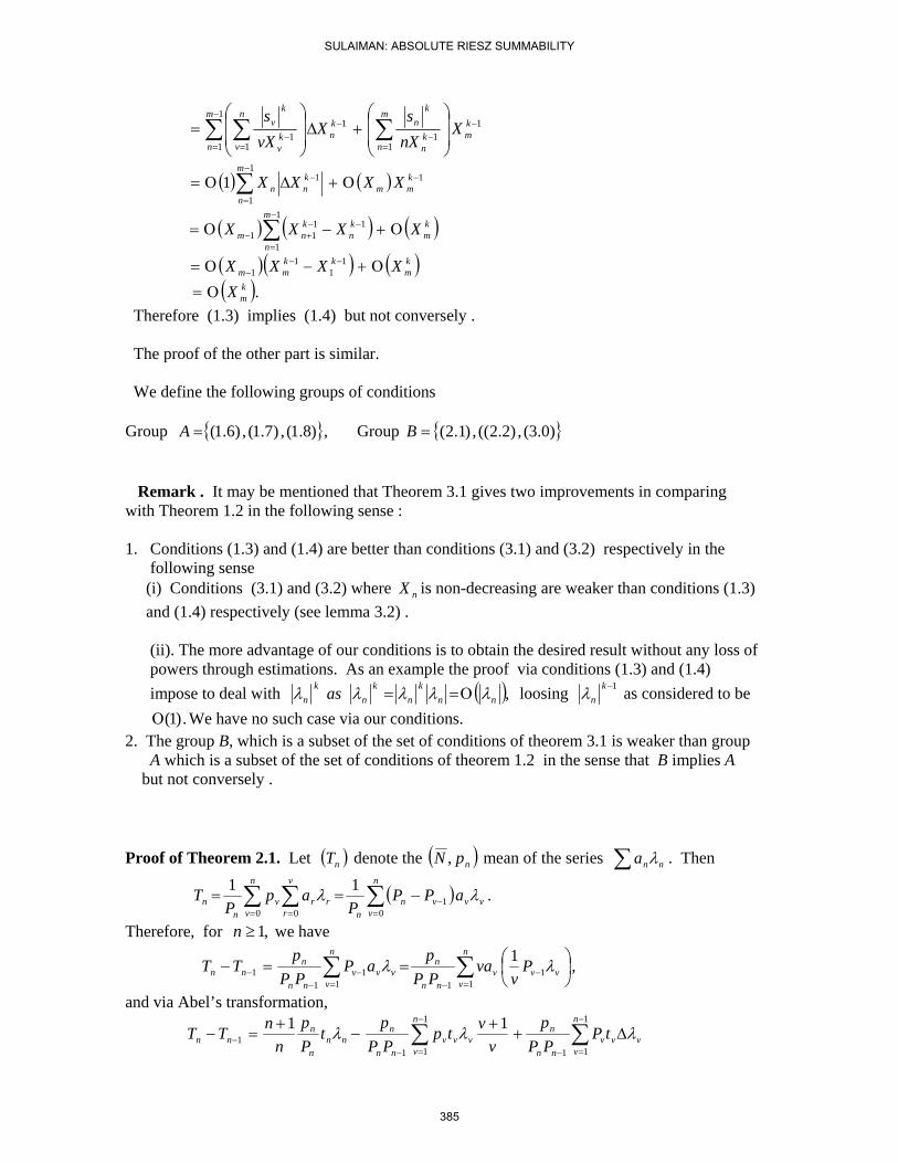
1
11
1
1
1
11
−
=−
−
=
−
=− ⎟
⎟
⎠
⎞
⎜⎜
⎝
⎛+∆
⎟⎟
⎠
⎞
⎜⎜
⎝
⎛= ∑∑ ∑ k
m
m
nkn
kn
m
n
kn
n
vkv
kv X
nXs
XvXs
( ) ( ) 111
1
1 −−−
=
Ο+∆Ο= ∑ kmm
kn
m
nn XXXX
( ) ( ) ( )km
m
n
kn
knm XXXX Ο+−Ο= ∑
−
=
−−+−
1
1
1111
( )( ) ( )km
kkmm XXXX Ο+−Ο= −−
−1
11
1 ( ).k
mXΟ= Therefore (1.3) implies (1.4) but not conversely . The proof of the other part is similar. We define the following groups of conditions Group )8.1(,)7.1(,)6.1(=A , Group )0.3(,)2.2((,)1.2(=B
Remark . It may be mentioned that Theorem 3.1 gives two improvements in comparing with Theorem 1.2 in the following sense : 1. Conditions (1.3) and (1.4) are better than conditions (3.1) and (3.2) respectively in the
following sense (i) Conditions (3.1) and (3.2) where nX is non-decreasing are weaker than conditions (1.3) and (1.4) respectively (see lemma 3.2) .
(ii). The more advantage of our conditions is to obtain the desired result without any loss of powers through estimations. As an example the proof via conditions (1.3) and (1.4) impose to deal with ( ),nn
kn
kn
kn as λλλλλ Ο== loosing 1−k
nλ as considered to be .)1(Ο We have no such case via our conditions.
2. The group B, which is a subset of the set of conditions of theorem 3.1 is weaker than group A which is a subset of the set of conditions of theorem 1.2 in the sense that B implies A but not conversely .
Proof of Theorem 2.1. Let ( )nT denote the ( )npN , mean of the series ∑ nna λ . Then
( ) .110
100
vv
n
vvn
n
v
rrr
n
vv
nn aPP
Pap
PT λλ ∑∑∑
=−
==
−==
Therefore, for ,1≥n we have
⎟⎠⎞
⎜⎝⎛==− −
=−=−
−− ∑∑ vv
n
vv
nn
nn
vvvv
nn
nnn P
vva
PPp
aPPPp
TT λλ 1111
11
11 ,
and via Abel’s transformation,
∑∑−
=−
−
=−− ∆+
+−
+=−
1
11
1
111
11 n
vvvv
nn
nn
vvvv
nn
nnn
n
nnn tP
PPp
vvtp
PPp
tPp
nnTT λλλ
SULAIMAN: ABSOLUTE RIESZ SUMMABILITY
385
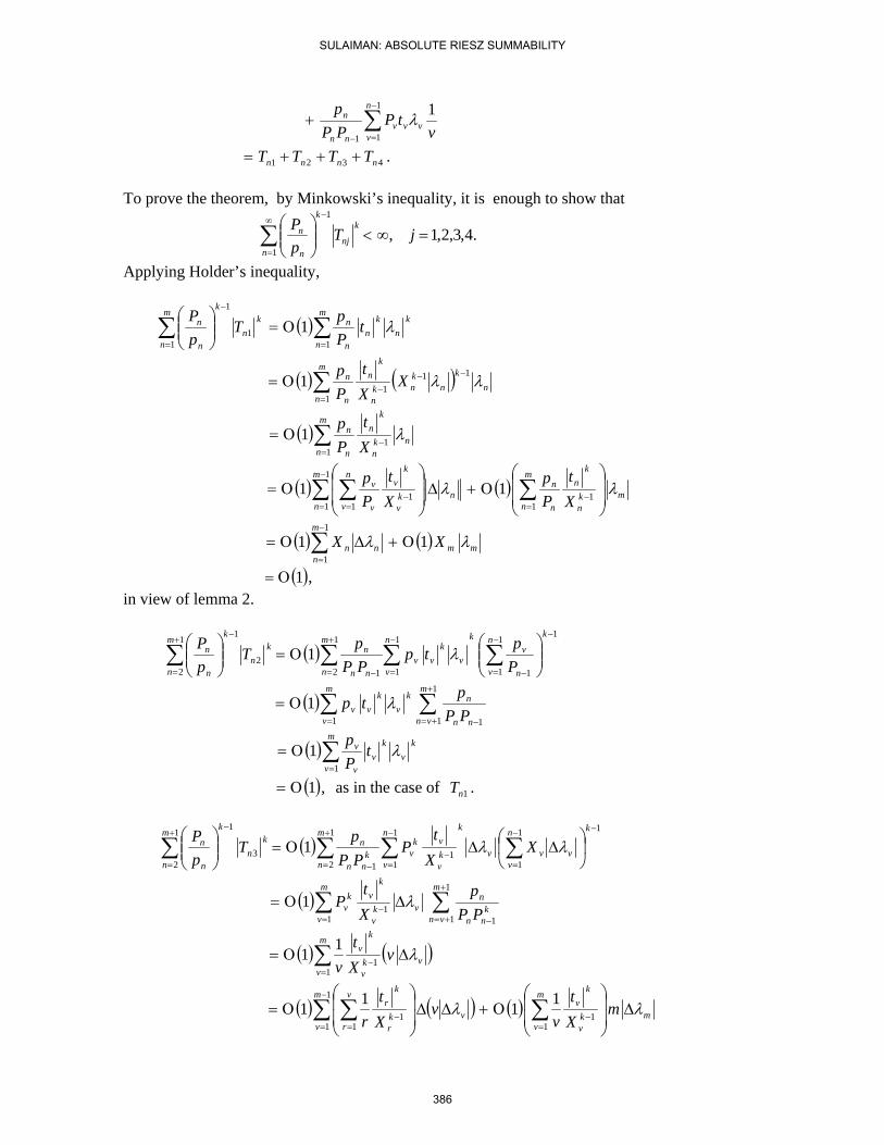
∑−
=−
+1
11
1n
vvvv
nn
n
vtP
PPp
λ
.4321 nnnn TTTT +++= To prove the theorem, by Minkowski’s inequality, it is enough to show that
.4,3,2,1,1
1
=∞<⎟⎟⎠
⎞⎜⎜⎝
⎛−
∞
=∑ jT
pP k
nj
k
n n
n
Applying Holder’s inequality,
( ) kn
kn
m
n n
nm
n
kn
k
n
n tPp
TpP
λ∑∑==
−
Ο=⎟⎟⎠
⎞⎜⎜⎝
⎛
111
1
1
( ) ( ) nk
nknk
n
kn
m
n n
n XXt
Pp
λλ11
11
1 −−−
=∑Ο=
( ) nkn
kn
m
n n
n
Xt
Pp
λ11
1 −=∑Ο=
( ) ( ) mkn
kn
m
n n
nn
m
n
n
vkv
kv
v
v
Xt
Pp
Xt
Pp
λλ⎟⎟
⎠
⎞
⎜⎜
⎝
⎛Ο+∆
⎟⎟
⎠
⎞
⎜⎜
⎝
⎛Ο= −
=
−
= =− ∑∑ ∑ 1
1
1
1 11 11
( ) ( ) mmn
m
nn XX λλ 11
1
1
Ο+∆Ο= ∑−
=
( ),1Ο= in view of lemma 2.
( )11
1 1
1
1
1
2 1
1
22
1
1−
−
= −
−
=
+
= −
+
=
−
⎟⎟⎠
⎞⎜⎜⎝
⎛Ο=⎟⎟
⎠
⎞⎜⎜⎝
⎛∑∑∑∑
kn
v n
vkn
vv
kvv
m
n nn
nm
n
kn
k
n
n
Pp
tpPPp
TpP
λ
( ) ∑∑+
+= −=
Ο=1
1 11
1m
vn nn
nkv
m
v
kvv PP
ptp λ
( ) kv
kv
m
v v
v tPp
λ∑=
Ο=1
1
( ),1Ο= as in the case of .1nT
( )11
1
1
11
1
2 13
1
2
1
1−−
=
−
=−
+
= −
+
=
−
⎟⎠
⎞⎜⎝
⎛∆∆Ο=⎟⎟
⎠
⎞⎜⎜⎝
⎛∑∑∑∑
k
v
n
vvv
kn
vkv
vkv
m
nk
nn
nkn
m
n
k
n
n XXt
PPPp
TpP
λλ
( ) ∑∑+
+= −−
=
∆Ο=1
1 11
1
1m
vnk
nn
nvk
v
kv
m
v
kv PP
pXt
P λ
( ) ( )v
m
vkv
kv v
Xt
vλ∆Ο= ∑
=−
11
11
( ) ( ) ( ) m
m
vkv
kv
v
m
v
v
rkr
kr m
Xt
vv
Xt
rλλ ∆
⎟⎟
⎠
⎞
⎜⎜
⎝
⎛Ο+∆∆
⎟⎟
⎠
⎞
⎜⎜
⎝
⎛Ο= ∑∑ ∑
=−
−
= =−
11
1
1 11
1111
SULAIMAN: ABSOLUTE RIESZ SUMMABILITY
386

( ) ( )( ) ( ) mmvv
m
vv mXvX λλλ ∆Ο+∆∆++∆−Ο= ∑
−
=
1111
1
( ) ( ) ( ) mm
m
vvvv
m
vv mXvXX λλλ ∆Ο+∆∆Ο+∆Ο= ∑∑
==
11111
( ).1Ο=
( )1`1
1
1
1
1
2 14
11
2
1−−
=
−
=
+
= −
−+
=
⎟⎠
⎞⎜⎝
⎛Ο=⎟⎟
⎠
⎞⎜⎜⎝
⎛∑∑∑∑
kn
v
vkv
kv
n
v
vm
nk
nn
nkn
km
n n
n
vP
tv
PPPp
TpP
λ
( ) ∑∑+
+= −=
Ο=1
1 111
m
vn nn
nkv
kv
m
v
v
PPp
tv
Pλ
( ) ∑∑+
+= −=
Ο=1
1 111
m
vn nn
nkv
kv
m
v
v
PPp
tv
Pλ
( )1Ο= ( ) vk
vvkv
kv
m
vX
Xt
vλλ
1
11
1 −
−=∑
( ) vkv
kv
m
v Xt
vλ1
1
11 −=∑Ο=
( ) ( ) mkv
kv
m
vv
m
v
v
rkr
kr
Xt
vXt
rλλ
⎟⎟
⎠
⎞
⎜⎜
⎝
⎛Ο+∆
⎟⎟
⎠
⎞
⎜⎜
⎝
⎛Ο= −
=
−
= =− ∑∑ ∑ 1
1
1
1 11
1111
( ) ( ) mmv
m
vv XX λλ 11
1Ο+∆Ο= ∑
=
( ).1Ο= This completes the proof of the theorem .
References [1] H. Bor, A note on two summability methods, Proc. Amer. Math. Soc. 98 (1986), 81-84. [2] H. Bor and L. Debnath, Quasi −β power increasing sequences, Internal. J. And Math. Sci., 44 (2004), 2371-2376. [3] T. M. Flett, On an extension of absolute summability and some theorems of Littlewood and Paley, Proc. London Math. Soc. 7 (1957) 113- 141. [4] L. Leindler, A recent note on the absolute Riesz summability factors, J. Ineq. Pure Appl. Math. Volume 7, Issue 2, Article 44, 2006. [5] W. T. Sulaiman, Extension on absolute summability factors of infinite series, J. Math. Anal. Appl. 322 (2006), 1224-1230.
SULAIMAN: ABSOLUTE RIESZ SUMMABILITY
387
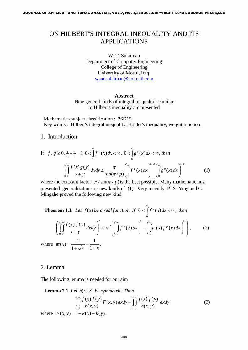
ON HILBERT'S INTEGRAL INEQUALITY AND ITS APPLICATIONS
W. T. Sulaiman
Department of Computer Engineering College of Engineering
University of Mosul, Iraq. [email protected]
Abstract New general kinds of integral inequalities similar
to Hilbert's inequality are presented Mathematics subject classification : 26D15. Key words : Hilbert's integral inequality, Holder's inequality, weight function.
1. Introduction
If thendxxgdxxfgf qpqp ,)(0,)(0,1,0,
00
11 ∞<<∞<<=+≥ ∫∫∞∞
q
q
p
p dxxgdxxfp
dxdyyx
ygxf/1
0
/1
00 0
)()()/sin(
)()(⎟⎟⎠
⎞⎜⎜⎝
⎛⎟⎟⎠
⎞⎜⎜⎝
⎛≤
+ ∫∫∫ ∫∞∞∞ ∞
ππ (1)
where the constant factor )/sin(/ pππ is the best possible. Many mathematicians presented generalizations or new kinds of (1). Very recently P. X. Ying and G. Mingzhe proved the following new kind
Theorem 1.1. Let )(xf be a real function. If ,)(00
2 ∞<< ∫∞
dxxf then
⎟⎟
⎠
⎞
⎜⎜
⎝
⎛⎟⎟⎠
⎞⎜⎜⎝
⎛−⎟⎟
⎠
⎞⎜⎜⎝
⎛<⎟⎟
⎠
⎞⎜⎜⎝
⎛
+ ∫∫∫ ∫∞∞∞ ∞ 2
0
2
0
2
2
0 0
)()()()()( dxxfxdxxfdxdyyx
yfxf pp ϖπ , (2)
where .1
11
1)(xx
x+
−+
=ϖ
2. Lemma The following lemma is needed for our aim Lemma 2.1. Let ),( yxh be symmetric. Then
dxdyyxh
yfxfdxdyyxFyxh
yfxf∫ ∫∫ ∫∞ ∞∞ ∞
=0 00 0 ),(
)()(),(),(
)()( (3)
where .)()(1),( ykxkyxF +−=
388
JOURNAL OF APPLIED FUNCTIONAL ANALYSIS, VOL.7, NO. 4,388-393,COPYRIGHT 2012 EUDOXUS PRESS,LLC
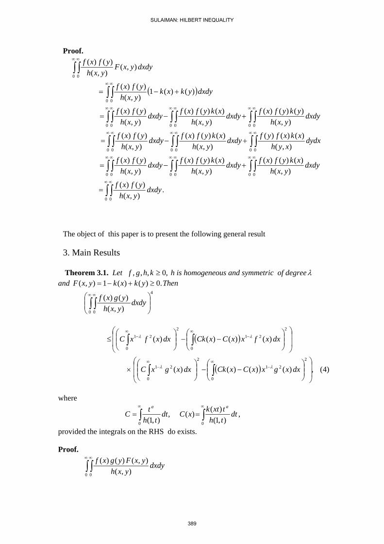
Proof.
dxdyyxFyxh
yfxf ),(),(
)()(
0 0∫ ∫∞ ∞
( )dxdyykxkyxh
yfxf )()(1),(
)()(
0 0
+−= ∫ ∫∞ ∞
dxdyyxh
ykyfxfdxdyyxh
xkyfxfdxdyyxh
yfxf∫ ∫∫ ∫∫ ∫∞ ∞∞ ∞∞ ∞
+−=0 00 00 0 ),(
)()()(),(
)()()(),(
)()(
dydxxyh
xkxfyfdxdyyxh
xkyfxfdxdyyxh
yfxf∫ ∫∫ ∫∫ ∫∞ ∞∞ ∞∞ ∞
+−=0 00 00 0 ),(
)()()(),(
)()()(),(
)()(
dxdyyxh
xkyfxfdxdyyxh
xkyfxfdxdyyxh
yfxf∫ ∫∫ ∫∫ ∫∞ ∞∞ ∞∞ ∞
+−=0 00 00 0 ),(
)()()(),(
)()()(),(
)()(
.),(
)()(
0 0
dxdyyxh
yfxf∫ ∫∞ ∞
=
The object of this paper is to present the following general result 3. Main Results
Theorem 3.1. Let ,0,,, ≥khgf h is homogeneous and symmetric of degreeλ and .0)()(1),( ≥+−= ykxkyxF Then
4
0 0 ),()()(
⎟⎟⎠
⎞⎜⎜⎝
⎛∫ ∫∞ ∞
dxdyyxh
ygxf
( )
( ) )4(,)()()()(
)()()()(
2
21
0
2
0
21
2
21
0
2
0
21
⎟⎟
⎠
⎞
⎜⎜
⎝
⎛⎟⎟⎠
⎞⎜⎜⎝
⎛−−⎟⎟
⎠
⎞⎜⎜⎝
⎛×
⎟⎟
⎠
⎞
⎜⎜
⎝
⎛⎟⎟⎠
⎞⎜⎜⎝
⎛−−⎟⎟
⎠
⎞⎜⎜⎝
⎛≤
−∞∞
−
−∞∞
−
∫∫
∫∫
dxxgxxCxCkdxxgxC
dxxfxxCxCkdxxfxC
λλ
λλ
where
,),1(
)()(,),1( 00
dtthtxtkxCdt
thtC
aa
∫∫∞∞
==
provided the integrals on the RHS do exists. Proof.
dxdyyxh
yxFygxf∫ ∫∞ ∞
0 0 ),(),()()(
SULAIMAN: HILBERT INEQUALITY
389

dxdyyxh
yxFygyxh
yxFxf),(
),()(),(
),()(
0 0
×= ∫ ∫∞ ∞
2/1
0 0
22/1
0 0
2
),(),()(
),(),()(
⎟⎟⎠
⎞⎜⎜⎝
⎛⎟⎟⎠
⎞⎜⎜⎝
⎛≤ ∫ ∫∫ ∫
∞ ∞∞ ∞
dxdyyxh
yxFygdxdyyxh
yxFxf
.NM=
dxdyyx
yxhyxFxf
xy
yxhyxFxf
Maa 2/
0 0
2/
),(),()(
),(),()(
⎟⎟⎠
⎞⎜⎜⎝
⎛×⎟
⎠⎞
⎜⎝⎛= ∫ ∫
∞ ∞
2/1
0 0
22/1
0 0
2
),(),()(
),(),()(
⎟⎟
⎠
⎞
⎜⎜
⎝
⎛⎟⎟⎠
⎞⎜⎜⎝
⎛⎟⎟⎠
⎞⎜⎜⎝
⎛⎟⎠⎞
⎜⎝⎛≤ ∫ ∫∫ ∫
∞ ∞∞ ∞
dxdyyx
yxhyxFxfdxdy
xy
yxhyxFxf
aa
.21 MM=
( ) dxdyxy
yxhykxkxfM
a
⎟⎠⎞
⎜⎝⎛+−
= ∫ ∫∞ ∞
0 0
2
1 ),()()(1)(
( ) ( ) ( ) dydxyxh
xyykxfdydxyxh
xyxkxfaa
∫∫∫∫∞∞∞∞
+−=00
2
00
2
),(/)()(
),(/)(1)(
( ) dudxuh
uxfxkxa
∫∫∞∞
− −=00
21
),1()()(1λ
dudxuhxukuxfx
a
∫∫∞∞
−+00
21
),1()()(λ
( ) .)()()()( 21
00
21 dxxfxxCxCkdxxfxC λλ −∞∞
− ∫∫ −−=
Similarly,
( ) .)()()()( 21
00
212 dxxfxxCxCkdxxfxCM λλ −
∞∞− ∫∫ −+=
Therefore
( ) ,)()()()(2
21
0
2
0
212⎟⎟⎠
⎞⎜⎜⎝
⎛−−⎟⎟
⎠
⎞⎜⎜⎝
⎛= −
∞∞− ∫∫ dxxfxxCxCkdxxfxCM λλ
and
( ) .)()()()(2
21
0
2
0
212⎟⎟⎠
⎞⎜⎜⎝
⎛−−⎟⎟
⎠
⎞⎜⎜⎝
⎛= −
∞∞− ∫∫ dxxgxxCxCkdxxgxCN λλ
Applying lemma 2.1 to have
4
0 0
4
0 0 ),(),()()(
),()()(
⎟⎟⎠
⎞⎜⎜⎝
⎛=⎟⎟
⎠
⎞⎜⎜⎝
⎛∫ ∫∫ ∫∞ ∞∞ ∞
dxdyyxh
yxFygxfdxdyyxh
ygxf
SULAIMAN: HILBERT INEQUALITY
390
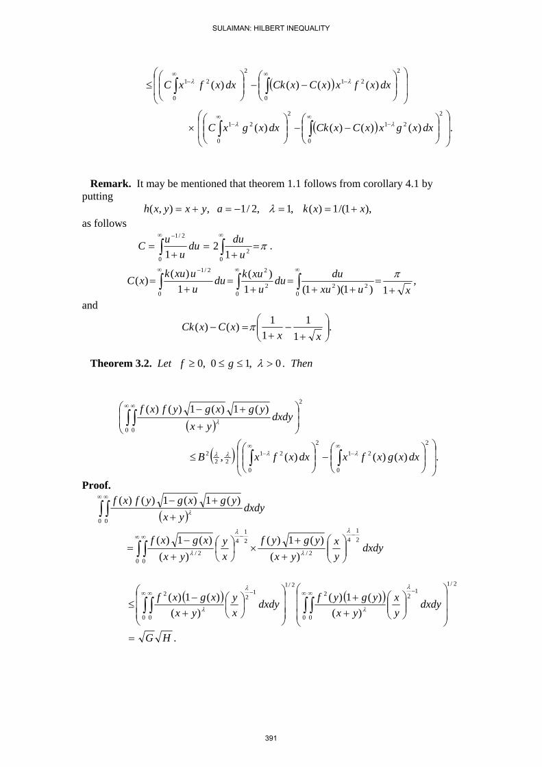
( )
( ) .)()()()(
)()()()(
2
21
0
2
0
21
2
21
0
2
0
21
⎟⎟
⎠
⎞
⎜⎜
⎝
⎛⎟⎟⎠
⎞⎜⎜⎝
⎛−−⎟⎟
⎠
⎞⎜⎜⎝
⎛×
⎟⎟
⎠
⎞
⎜⎜
⎝
⎛⎟⎟⎠
⎞⎜⎜⎝
⎛−−⎟⎟
⎠
⎞⎜⎜⎝
⎛≤
−∞∞
−
−∞∞
−
∫∫
∫∫
dxxgxxCxCkdxxgxC
dxxfxxCxCkdxxfxC
λλ
λλ
Remark. It may be mentioned that theorem 1.1 follows from corollary 4.1 by putting ),1/(1)(,1,2/1,),( xxkayxyxh +==−=+= λ as follows
π=+
=+
= ∫∫∞∞ −
02
0
2/1
12
1 ududu
uuC .
,1)1)(1(1
)(1
)()(0
220
2
2
0
2/1
xuxududu
uxukdu
uuxukxC
+=
++=
+=
+= ∫∫∫
∞∞∞ − π
and
.1
11
1)()( ⎟⎟⎠
⎞⎜⎜⎝
⎛+
−+
=−xx
xCxCk π
Theorem 3.2. Let 0,10,0 >≤≤≥ λgf . Then
( )
2
0 0
)(1)(1)()(⎟⎟⎠
⎞⎜⎜⎝
⎛
+
+−∫ ∫∞ ∞
dxdyyx
ygxgyfxfλ
( ) .)()()(,2
0
21
2
0
2122
2
⎟⎟
⎠
⎞
⎜⎜
⎝
⎛⎟⎟⎠
⎞⎜⎜⎝
⎛−⎟⎟
⎠
⎞⎜⎜⎝
⎛≤ ∫∫
∞−
∞− dxxgxfxdxxfxB λλλλ
Proof.
( )
dxdyyx
ygxgyfxf∫ ∫∞ ∞
++−
0 0
)(1)(1)()(λ
dxdyyx
yxygyf
xy
yxxgxf 2
14
2/
21
4
0 02/ )(
)(1)()(
)(1)( −−∞ ∞
⎟⎟⎠
⎞⎜⎜⎝
⎛+
+×⎟
⎠⎞
⎜⎝⎛
+−
= ∫ ∫λ
λ
λ
λ
( ) ( )2/1
0 0
122
2/1
0 0
122
)()(1)(
)()(1)(
⎟⎟⎟
⎠
⎞
⎜⎜⎜
⎝
⎛
⎟⎟⎠
⎞⎜⎜⎝
⎛++
⎟⎟⎟
⎠
⎞
⎜⎜⎜
⎝
⎛⎟⎠⎞
⎜⎝⎛
+−
≤ ∫ ∫∫ ∫∞ ∞ −∞ ∞ −
dxdyyx
yxygyfdxdy
xy
yxxgxf
λ
λ
λ
λ
.HG=
SULAIMAN: HILBERT INEQUALITY
391
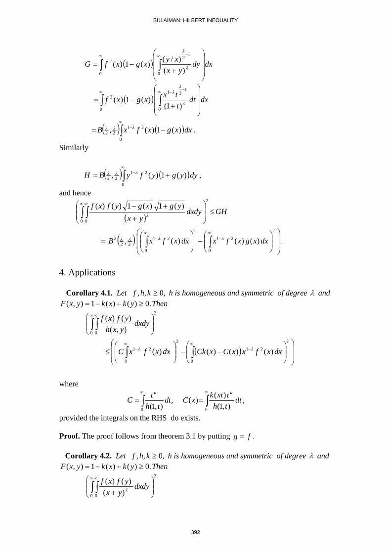
( ) dxdyyx
xyxgxfG⎟⎟⎟
⎠
⎞
⎜⎜⎜
⎝
⎛
+−= ∫∫
∞ −∞
0
12
0
2
)()/()(1)( λ
λ
( ) dxdtttxxgxf
⎟⎟⎟
⎠
⎞
⎜⎜⎜
⎝
⎛
+−= ∫∫
∞ −−∞
0
121
0
2
)1()(1)( λ
λλ
( ) ( )∫∞
− −=0
2122 )(1)(, dxxgxfxB λλλ .
Similarly
( ) ( )∫∞
− +=0
2122 )(1)(, dyygyfyBH λλλ ,
and hence
( )
( ) .)()()(,
)(1)(1)()(
2
0
21
2
0
2122
2
2
0 0
⎟⎟
⎠
⎞
⎜⎜
⎝
⎛⎟⎟⎠
⎞⎜⎜⎝
⎛−⎟⎟
⎠
⎞⎜⎜⎝
⎛=
≤⎟⎟⎠
⎞⎜⎜⎝
⎛
+
+−
∫∫
∫ ∫∞
−∞
−
∞ ∞
dxxgxfxdxxfxB
GHdxdyyx
ygxgyfxf
λλλλ
λ
4. Applications Corollary 4.1. Let ,0,, ≥khf h is homogeneous and symmetric of degree λ and
.0)()(1),( ≥+−= ykxkyxF Then
2
0 0 ),()()(
⎟⎟⎠
⎞⎜⎜⎝
⎛∫ ∫∞ ∞
dxdyyxh
yfxf
( ) ⎟
⎟
⎠
⎞
⎜⎜
⎝
⎛⎟⎟⎠
⎞⎜⎜⎝
⎛−−⎟⎟
⎠
⎞⎜⎜⎝
⎛≤ −
∞∞− ∫∫
2
21
0
2
0
21 )()()()( dxxfxxCxCkdxxfxC λλ
where
,),1(
)()(,),1( 00
dtthtxtkxCdt
thtC
aa
∫∫∞∞
==
provided the integrals on the RHS do exists. Proof. The proof follows from theorem 3.1 by putting .fg = Corollary 4.2. Let ,0,, ≥khf h is homogeneous and symmetric of degree λ and
.0)()(1),( ≥+−= ykxkyxF Then
2
0 0 )()()(
⎟⎟⎠
⎞⎜⎜⎝
⎛
+∫ ∫∞ ∞
dxdyyx
yfxfλ
SULAIMAN: HILBERT INEQUALITY
392
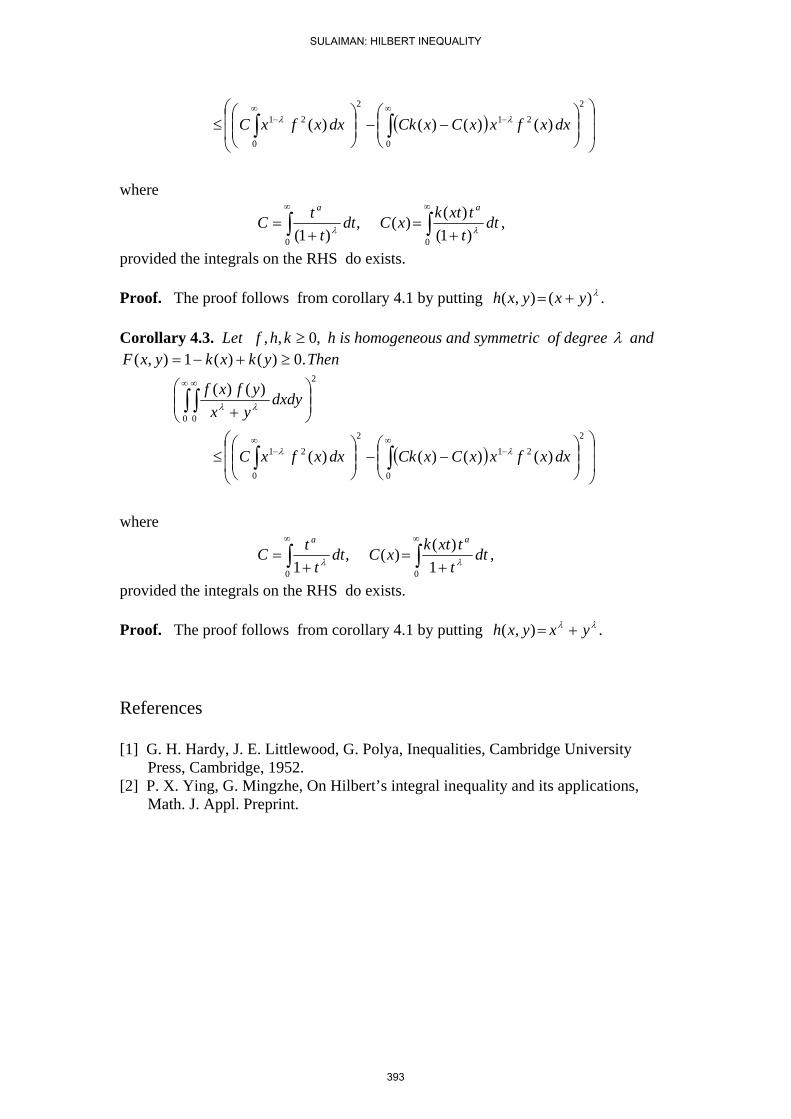
( ) ⎟
⎟
⎠
⎞
⎜⎜
⎝
⎛⎟⎟⎠
⎞⎜⎜⎝
⎛−−⎟⎟
⎠
⎞⎜⎜⎝
⎛≤ −
∞∞− ∫∫
2
21
0
2
0
21 )()()()( dxxfxxCxCkdxxfxC λλ
where
,)1(
)()(,)1( 00
dtttxtkxCdt
ttC
aa
∫∫∞∞
+=
+= λλ
provided the integrals on the RHS do exists. Proof. The proof follows from corollary 4.1 by putting .)(),( λyxyxh += Corollary 4.3. Let ,0,, ≥khf h is homogeneous and symmetric of degree λ and
.0)()(1),( ≥+−= ykxkyxF Then
2
0 0
)()(⎟⎟⎠
⎞⎜⎜⎝
⎛
+∫ ∫∞ ∞
dxdyyx
yfxfλλ
( ) ⎟
⎟
⎠
⎞
⎜⎜
⎝
⎛⎟⎟⎠
⎞⎜⎜⎝
⎛−−⎟⎟
⎠
⎞⎜⎜⎝
⎛≤ −
∞∞− ∫∫
2
21
0
2
0
21 )()()()( dxxfxxCxCkdxxfxC λλ
where
,1
)()(,1 00
dtttxtkxCdt
ttC
aa
∫∫∞∞
+=
+= λλ
provided the integrals on the RHS do exists. Proof. The proof follows from corollary 4.1 by putting .),( λλ yxyxh +=
References [1] G. H. Hardy, J. E. Littlewood, G. Polya, Inequalities, Cambridge University Press, Cambridge, 1952. [2] P. X. Ying, G. Mingzhe, On Hilbert’s integral inequality and its applications, Math. J. Appl. Preprint.
SULAIMAN: HILBERT INEQUALITY
393

Optimal Source for Maximum Distinguishability in Optical Imaging
Bonnie Jacob∗ Bangti Jin† Taufiquar Khan∗ Peter Maass†
December 15, 2010
Abstract
In this paper, we formulate an optimal source problem for optical imaging by maximizingeight different distinguishability criteria. Each distinguishability criterion represents one of theeight pairs of function spaces considered. We extend the general concept of finding an optimalcurrent for a particular distinguishability criterion, as in electrical impedance imaging, to anoptimal source in optical imaging.
The optimal source depends on the distinguishability criterion which in turn depends onthe choice of the function space pairs. We shall provide an analytic framework for computingall these eight different choices of distinguishability criteria. In particular, the adjoints of therelevant linear operators involved in the criteria are derived.
Numerically, we employ the power method to compute the optimal sources, i.e. the dominanteigenfunctions of the associated operators. Numerical experiments are presented to demonstratethe efficacy of different criteria, and a localization measure is used to determine the optimalsource profile best discriminating inhomogeneities from a known background.
Keywords: distinguishability criteria, abstract function spaces, optimal source, optical imag-ing, biomedical imaging
1 Introduction
In optical imaging of highly scattering media such as biological tissue, the media is illuminated bylow-energy visible (wavelength from 380 to 750 nm) or near-infrared light (wavelength from 700to 1200 nm). Light penetrates the medium and interacts with it. The predominant effects areabsorption and scattering [12, 3, 10, 16]. The widely accepted photon transport model is the radia-tive transfer equation [5, 19], an integro-differential equation for the radiance, involving spatiallyvarying scattering and absorption parameters. In practice, a low order diffusion approximationto the radiative transfer equation is often adopted. The approximation is a parabolic differentialequation in the time-dependent case, while in the steady-state case or frequency domain, it is anelliptic differential equation [1, 2]. Most existing computational methods for photon transport inhighly scattering media such as photon migration in biological tissues are based on the diffusionapproximation because of its simplicity compared to the full blown radiative transfer equation[4, 17].
In the experimental setup of non-invasive diffuse optical imaging such as optical tomographyand other similar non-invasive imaging modalities, e.g. electrical impedance imaging, one has verylittle control over the parameters in the domain other than the boundary source. Therefore, the idea∗Department of Mathematical Sciences, Clemson University, Clemson, SC 29634-0975, USA ([email protected]).†Center for Industrial Mathematics, University of Bremen, D-28334 Bremen, Germany ([email protected]
bremen.de).
1394
JOURNAL OF APPLIED FUNCTIONAL ANALYSIS, VOL.7, NO. 4,394-412,COPYRIGHT 2012 EUDOXUS PRESS,LLC

of using an optimal source to maximize the distinguishability is an important step. For examplesuppose that Λ(q+)[f ] : X → Y is the source to data map where q+ represents the true parametersand Λ(q)[f ] : X → Y is the source to simulated data map for a guess q of the parameters. Then onemay use the following natural distinguishability criterion [18, 7], δXY (f) = ‖Λ(q)[f ]− Λ(q+)[f ]‖Yto find the best f that will discriminate between the simulated model and the measured data bysolving the following problem,
maxf∈X
δXY (f) = ‖Λ(q)[f ]− Λ(q+)[f ]‖Y (1)
where Λ : X → Y . The selection of an optimal source by maximizing a particular distinguishabilitycriterion has potential to lead to the following benefits:
(i) to improve image reconstruction in diffuse optical imaging applications. For example, thereexist numerous studies in electrical impedance tomography (EIT) that indicate that optimal cur-rents have the potential to improve the image reconstruction [18, 6, 22, 7]. It is expected thatthe above mentioned developments in EIT will have a similar impact for optical tomography (OT)[9, 14];
(ii) in formulating a statistical hypothesis testing problem to address the question of whetherthere is a tumor present or not. For example, one of the criteria studied in this paper correspondsto the maximum likelihood ratio test. Therefore our framework will also have applications in signaland image reconstruction [26];
(iii) for extracting features of the source-to-data operator using the outer product of the firstfew largest eigenvectors as an approximation of the operator. In addition, the characteristic profileof the optimal source may also correlate to the type of inhomogeneity present in the interior;
(iv) in developing a general framework to find optimal source for hybrid imaging modalities.It is expected that hybrid imaging techniques involving optical sources will develop rapidly in thecoming decade [15, 29, 28].
Therefore, the problem of finding an optimal source with maximum distinguishability is animportant and timely subject in optical imaging. In addition, the laser sources in optical imagingare more flexible in terms of tunability and adaptability [24, 25] than, for example, current sourcesin electrical impedance imaging. Hence, we expect an even stronger impact of using optimal sourcesin optical imaging. Furthermore, the tremendous growth and intense research in laser sources makea wide range of sources realistically achievable and consequently might improve image resolution[24, 25].
The idea of distinguishability criteria for optimal currents in EIT has been around for more thana decade [18, 13, 6, 22, 7]. However, a thorough investigation in a functional analytic frameworkinvolving all of the relevant function space pairs and numerical comparison of respective optimalcurrents are only getting attention very recently [20]. A careful reading of some of the literaturereferenced above both in electrical impedance and optical imaging indicate that most of thesepapers mention the general setup for various appropriate function spaces but then typically chooseone of them without fully analyzing the general case. It seems that this is done mainly to avoidcumbersome analytic calculations required to compute the optimal source.
In this paper we will formulate the distinguishability criteria for all eight relevant pairs of thefunction spaces for the operator of choice and demonstrate the general framework on how to handlethem both theoretically and computationally. In the numerical section we will then determine thefunction space setting most suitable in designing optimal sources for optical tomography experi-ments.
Let us summarize the current state of the art of optimal sources in diffuse optical imaging.There exist past and recent studies on how to optimize wavelength and frequency in optical image
2
JACOB ET AL: OPTIMAL SOURCE...OPTICAL IMAGING
395

reconstruction [9, 14], as well as on how to optimize location and power for sources and detectors[26]. However, none of these studies simultaneously consider all of the relevant function spaces pairs,and heuristic analysis is carried out on the discretized problem without analyzing the involvedfunction spaces. In this paper, we shall treat the infinite dimensional model and propose analgorithm to compute the optimal source with a finite dimensional approximation for every plausiblefunction space setting in a mathematically rigorous manner. In particular, we shall extend thedistinguishability criteria for optimal currents in impedance imaging to optimal sources in diffuseoptical imaging, systematically investigate the influence of function spaces on optimal sources bothanalytically and numerically, and determine the most effective pair of function spaces using alocalization measure.
The analytical work and the computational simulations presented in this paper involve eightfunction space pairs. Therefore in this paper, we have concentrated on the details of the appro-priate formulation relevant to our computational setup. We have presented relevant simulationsto demonstrate that the solutions for the different distinguishability criteria corresponding to thevarious function spaces differ. For convenience, in this paper, we only considered the Neumannand Dirichlet boundary conditions; however the analysis can be easily extended to any boundaryconditions including Robin boundary conditions. We note that the there are several questions thatrequire further analysis and are beyond the scope of this manuscript: (i) since distinguishabilityis a local measure, a theoretical and numerical sensitivity analysis of how the solution varies fromregion to region in the parameter space will be taken up in the future, (ii) the simulations presentedin the paper involve mainly model error due to discretization; however we do not take up the issueof effects due to finite dimensional projection or approximation, or the issue of uncertainty analysis.
The rest of the paper is organized as follows. We introduce relevant mathematical models anddescribe important function spaces in Section 2. In Section 2.2, we discuss the optimal source prob-lem. To numerically calculate the optimal sources of these distinguishability criteria, we determinethe adjoint of appropriate operators in Section 3, and in Section 4 we demonstrate the efficacy ofour approach using two-dimensional examples of optical imaging source optimization.
2 Mathematical Model and Distinguishability Criteria
In this section, we describe the mathematical model and introduce distinguishability criteria aswell as the functional analytical framework for properly formulating these models.
2.1 Mathematical model
Let Ω ⊂ IRd(d = 2, 3) be an open bounded domain with Lipschitz boundary ∂Ω. The diffusionapproximation model in the frequency domain for optical tomography can be written as
−∇ · (D∇u) + (µ+ ik)u = h in Ω,γ1u = f on ∂Ω,
(2)
where k = ω/c is the wave number with ω and c representing the frequency of laser modulationand light speed, respectively, and γ1 is the Neumann trace map, i.e. γ1u = D ∂u
∂ν . We furtherassume that D ∈ L∞(Ω) is the diffusion coefficient with 0 < D0 ≤ D(x) ≤ D1 < ∞ for positivereal constants D0 and D1, µ ∈ L∞(Ω) is the absorption coefficient with 0 < µ0 ≤ µ(x) ≤ µ1 < ∞for positive real constants µ0 and µ1, and f is a source function. We denote by q = (D,µ) theparameters, and by F (k,q)
N (h, f) the solution, which physically represents the photon density.
3
JACOB ET AL: OPTIMAL SOURCE...OPTICAL IMAGING
396
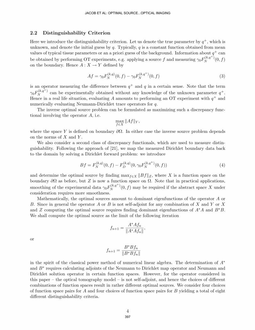
2.2 Distinguishability Criterion
Here we introduce the distinguishability criterion. Let us denote the true parameter by q+, which isunknown, and denote the initial guess by q. Typically, q is a constant function obtained from meanvalues of typical tissue parameters or an a priori guess of the background. Information about q+ canbe obtained by performing OT experiments, e.g. applying a source f and measuring γ0F
(k,q+)N (0, f)
on the boundary. Hence A : X → Y defined by
Af = γ0F(k,q)N (0, f)− γ0F
(k,q+)N (0, f) (3)
is an operator measuring the difference between q+ and q in a certain sense. Note that the termγ0F
(k,q+)N can be experimentally obtained without any knowledge of the unknown parameter q+.
Hence in a real life situation, evaluating A amounts to performing an OT experiment with q+ andnumerically evaluating Neumann-Dirichlet trace operators for q.
The inverse optimal source problem can be formulated as maximizing such a discrepancy func-tional involving the operator A, i.e.
maxf∈X‖Af‖Y ,
where the space Y is defined on boundary ∂Ω. In either case the inverse source problem dependson the norms of X and Y .
We also consider a second class of discrepancy functionals, which are used to measure distin-guishability. Following the approach of [21], we map the measured Dirichlet boundary data backto the domain by solving a Dirichlet forward problem: we introduce
Bf = F(k,q)N (0, f)− F (k,q)
D (0, γ0F(k,q+)N (0, f)) (4)
and determine the optimal source by finding maxf∈X ‖Bf‖Z , where X is a function space on theboundary ∂Ω as before, but Z is now a function space on Ω. Note that in practical applications,smoothing of the experimental data γ0F
(k,q+)N (0, f) may be required if the abstract space X under
consideration requires more smoothness.Mathematically, the optimal sources amount to dominant eigenfunctions of the operator A or
B. Since in general the operator A or B is not self-adjoint for any combination of X and Y or Xand Z computing the optimal source requires finding dominant eigenfunctions of A∗A and B∗B.We shall compute the optimal source as the limit of the following iteration
fn+1 =A∗Afn‖A∗Afn‖
,
or
fn+1 =B∗Bfn‖B∗Bfn‖
in the spirit of the classical power method of numerical linear algebra. The determination of A∗
and B∗ requires calculating adjoints of the Neumann to Dirichlet map operator and Neumann andDirichlet solution operator in certain function spaces. However, for the operator considered inthis paper – the optical tomography model – is not self-adjoint, and hence the choices of differentcombinations of function spaces result in rather different optimal sources. We consider four choicesof function space pairs for A and four choices of function space pairs for B yielding a total of eightdifferent distinguishability criteria.
4
JACOB ET AL: OPTIMAL SOURCE...OPTICAL IMAGING
397

2.3 Sesquilinear Weak Formulation
We shall use the following sesquilinear form
a(k,q)(u, v) =∫
ΩD∇u · ∇v + (µ+ ik)uvdx.
The weak formulation of the Neumann forward problem (2) now reads: find u ∈ H1(Ω) such thatfor all v ∈ H1(Ω)
a(k,q)(u, v) =∫
Ωhvdx+
∫∂Ωfγ0vds. (5)
The measurement g is modeled as the photon density u at the boundary, i.e.,
g = u|∂Ω = γ0u (6)
where γ0 : H1(Ω)→ H1/2(∂Ω) denotes the Dirichlet trace operator. With the measurement g, wecan define a nonhomogeneous Dirichlet boundary value problem as follows,
−∇ · (D∇u) + (µ+ ik)u = h in Ω,γ0u = g on ∂Ω.
(7)
We denote the Dirichlet solution u by F (k,q)D (h, g). Its weak formulation is given by: find u ∈ H1(Ω)
with γ0u = g such that
a(k,q)(u, v) =∫
Ωhvdx ∀v ∈ H1
0 (Ω). (8)
Observe that F (k,q)D (h, g) = F
(k,q)N (h, γ1F
(k,q)D (h, g)), and thus by the weak formulation of F (k,q)
N ,there holds: for any v ∈ H1(Ω)
a(k,q)(F (k,q)D (h, g), v) =
∫Ωhvdx+
∫∂Ωγ1F
(k,q)D (h, g)vds.
This formula will be used several times in Section 3.We mainly consider boundary value problems (2) and (7) with vanishing h, and the correspond-
ing weak formulations (5) and (8). We will at times consider these boundary value problems butwith k = 0 or opposite signs for k, which shall be denoted by e.g. F (0,q)
N (h, f) and F(−k,q)N (h, f).
Finally, we let L(k,q)u = −∇ · (D∇u) + (µ+ ik)u.
2.4 Function spaces
To investigate the mathematical models, we shall utilize a Hilbert space framework [11, 8]. Firstwe equip the space H1
q (Ω) with an inner product
〈u, v〉H1q (Ω) =
∫ΩD∇u · ∇v + µuvdx (9)
where the bar denotes taking complex conjugate. The dual of H1q (Ω) will be denoted by H−1
q (Ω).
Then we define an inner product for H1/2q (∂Ω) by
〈f, g〉H
1/2q (∂Ω)
= 〈F (0,q)D (0, f), F (0,q)
D (0, g)〉H1q (Ω).
5
JACOB ET AL: OPTIMAL SOURCE...OPTICAL IMAGING
398
By appealing to the weak formulation of F (0,q)D (0, f) = F
(0,q)N (0, γ1F
(0,q)D (0, f)), we can equivalently
write〈f, g〉H1/2(∂Ω) =
∫∂Ωγ1F
(0,q)D (0, f)gds =
∫∂Ωfγ1F
(0,q)D (0, g)ds.
Similarly, we define the H−1/2q (∂Ω) inner product by
〈f, g〉H−1/2q (∂Ω)
= 〈F (0,q)N (0, f), F (0,q)
N (0, g)〉H1q (Ω)
and equivalently
〈f, g〉H−1/2q (∂Ω)
=∫∂Ωfγ0F
(0,q)N (0, g)ds =
∫∂Ωγ0F
(0,q)N (0, f)gds.
We would like to point out that the spaces H1/2q (∂Ω) and H−1/2
q (∂Ω) defined above are dual toeach other, and thus the integrals on the boundary can be understood as duality pairings as usual.
2.5 Riesz representation of the sesquilinear form
The following Riesz representation of the sesquilinear form a(k,q)(u, v) in (5) will be needed in thesubsequent sections. By virtue of the Riesz representation theorem for sesquilinear functionals [8],we deduce that there exists a unique continuous bijection S : H1
q (Ω) → H1q (Ω) such that for any
u, v ∈ H1q (Ω) there holds
a(k,q)(u, v) = 〈Su, v〉H1q (Ω) = 〈u, S∗v〉H1
q (Ω). (10)
The operator S depends on q and k, and the dependence is often suppressed. The representationoperator S and its adjoint S∗ can be explicitly characterized. The operator S will play a crucialrole in deriving the adjoints of various operators below.
Lemma 1. The operator S and its adjoint S∗ are given by Su = F(0,q)N (L(k,q)u, γ1u) and S∗v =
F(0,q)N (L(−k,q)v, γ1v), respectively. In particular, w = Su satisfies
−∇ · (D∇w) + µw = −∇ · (D∇u) + (µ+ ik)uγ1w = γ1u.
Proof. Let w = F(0,q)N (L(k,q)u, γ1u). By the definition of the H1(Ω) norm and its weak formulation
we have that for any v ∈ H1q (Ω)
〈w, v〉H1q (Ω) =
∫ΩL(k,q)uvdx+
∫∂Ωγ1uvds = a(u, v).
Thus Su = w = F(0,q)N (L(k,q)u, γ1u). The assertion for S∗ can be shown similarly.
The operators S and S∗ have some interesting properties. For a detailed discussion see [23]. Insubsequent sections we will need the following properties.
Lemma 2. Let u, v ∈ H1q (Ω), f, f ∈ H1/2
q (∂Ω), g ∈ H−1/2q (∂Ω) and h ∈ H−1
q (Ω). There hold
a) S∗F(−k,q)N (h, g) =F (0,q)
N (h, g) = SF(k,q)N (h, g),
b) γ1Su =γ1u = γ1S∗u,
c) 〈Su, S∗−1v〉H1q (Ω) =〈u, v〉H1
q (Ω),
d) f = γ0S−1(F (0,q)
D (0, f)) ⇐⇒ f = γ0SF(k,q)D (0, f).
6
JACOB ET AL: OPTIMAL SOURCE...OPTICAL IMAGING
399
Proof. The first two lines follow directly from Lemma 1, and c) follows from the definition of S andS∗. To see d), we observe from the characterization of S that f = γ0SF
(k,q)D (0, f) is equivalent to
f = γ0F(0,q)N (LkF (k,q)
D (0, f), γ1F(k,q)D (0, f)) = γ0F
(0,q)N (0, γ1F
(k,q)D (0, f)),
which consequently gives
F(0,q)D (0, f) = F
(0,q)N (0, γ1F
(k,q)D (0, f)) = SF
(k,q)D (0, f),
i.e.F
(k,q)D (0, f) = S−1F
(0,q)D (0, f).
Upon taking Dirichlet trace, it gives the desired assertion. The remaining parts follow similarly.
3 Adjoint Operators
The aim of this paper is to determine optimal source profiles for applications in optical imaging.To this end we compare measurements for the true parameter q+ with simulated measurementsobtained with an a priori guess q. As explained in Section 2, we use a functional analytic frameworkfor characterizing the optimal sources. This leads to the task of solving the problem,
max‖f‖X=1
‖Af‖Y
ormax‖f‖X=1
‖Bf‖Z
or equivalently of finding the largest eigenvalue of A∗A and B∗B. Here A measures the differencebetween the Neumann-to-Dirichlet maps for q+ and q. Similarly, B measures the difference betweenthe Dirichlet solution, in the full domain, corresponding to the experimental Neumann-to-Dirichletdata for q+ and the simulated solution, in the full domain, corresponding to a given guess q.
As we have seen already, we can use different function spaces for the domain of A : X → Y ,i.e. X = L2(∂Ω) or X = H−1/2(∂Ω), and two choices for the range of A, i.e. X = L2(∂Ω)or X = H1/2(∂Ω). Similarly, we can use different function spaces for the domain and range ofB : X → Z, i.e. X = L2(∂Ω) or X = H−1/2(∂Ω) and Z = L2(Ω) or Z = H1(Ω). The adjoint
A∗ : Y → X ,
which is determined via its defining relation 〈Af, g〉Y = 〈f,A∗g〉, depends on the choice of functionspaces and accordingly the resulting optimal sources will differ considerably, when computed forthose different function space settings. The same holds for the operator B.
First, in Section 3.1. we determine the adjoint operators for the two most natural function spacesettings for A. The general case for both A and B is discussed in Section 3.2. The computation ofadjoint operators is a standard exercise in functional analysis; however, our choice of norms, e.g.H1q (Ω), depends on the parameters q or q+, which leads to some subtle computations even for the
trivial embedding operators.
7
JACOB ET AL: OPTIMAL SOURCE...OPTICAL IMAGING
400
3.1 Adjoint operators for the classical functionals
In this section we address the computation of the adjoint operators for evaluating the distinguisha-bility criterion based on comparing the Neumann-to-Dirichlet maps for q and q+, as described in(3):
‖Af‖Y = ‖γ0F(k,q)N (0, f)− γ0F
(k,q+)N (0, f)‖Y .
We use the two natural function space settings
γ0F(k,q)N (0, ·) : L2(∂Ω)→ L2(∂Ω)
andγ0F
(k,q)N (0, ·) : H−1/2
q (∂Ω)→ H1/2q (∂Ω) .
In the second case, theH±1/2q norms depend in q, hence we have to consider the embedding operators
e− : H−1/2q (∂Ω)→ H
−1/2q+
(∂Ω) and e+ : H1/2q+
(∂Ω)→ H1/2q (∂Ω)
between spaces with parameters q = (D,µ) and q+ = (D+, µ+).Accordingly we must compute the adjoints of γ0F
(k,q)N (0, ·) and e+ γ0F
(k,q+)N (0, ·) e− before
obtaining a closed expression for A∗. This adjoint is then used in Section 4 for computing theoptimal sources.
We start by computing the adjoints of the Neumann-to-Dirichlet maps.
Lemma 3. Let Λ(k, q) = γ0F(k,q)N (0, ·) denote the Neumann-to-Dirichlet map. The adjoint of
Λ(k, q) : X → Y is given by
(a) Λ(k, q)∗g = γ0F(−k,q)N (0, g) for X = L2(∂Ω) and Y = L2(∂Ω);
(b) Λ(k, q)∗g = γ1F(0,q)D (0, γ0S
∗−1F(0,q)D (0, g)) for X = H
−1/2q (∂Ω) and Y = H
1/2q (∂Ω).
Proof. For the first case, we consider 〈Λ(k, q)f, g〉L2(∂Ω). By the weak formulations of F (−k,q)N (0, g)
and F(0,q)N (0, f), we derive
〈Λ(k, q)f, g〉L2(∂Ω) = 〈g,Λ(k, q)f〉L2(∂Ω)
= a(−k,q)(F (−k,q)N (0, g), F (k,q)
N (0, f))
= a(k,q)(F (k,q)N (0, f), F (−k,q)
N (0, g))
= 〈f, γ0F(−k,q)N (0, g)〉L2(∂Ω).
Hence we obtain Λ(k, q)∗ = Λ(−k, q).For proving the second case, we start with 〈Λ(k, q)f, g〉
H1/2q (∂Ω)
and use the definition of the norm
in H1/2q (∂Ω). Moreover, we apply the identity F (0,q)
D (0, γ0F(k,q)N (0, f)) = F
(k,q)N (0, f), which follows
from observing that the Dirichlet traces as well as the vanishing source terms coincide:
〈Λ(k, q)f, g〉H
1/2q (∂Ω)
= 〈F (0,q)D (0, γ0F
(k,q)N (0, f)), F (0,q)
D (0, g)〉H1q (Ω)
= 〈F (k,q)N (0, f), F (0,q)
D (0, g)〉H1q (Ω)
= a(0,q)(F (k,q)N (0, f), F (0,q)
D (0, g)).
8
JACOB ET AL: OPTIMAL SOURCE...OPTICAL IMAGING
401
We now apply the definition of S, see (10), and the weak formulation for F (k,q)N (0, f) to obtain
〈Λ(k, q)f, g〉H
1/2q (∂Ω)
= a(k,q)(F (k,q)N (0, f), S∗−1F
(0,q)D (0, g))
=∫∂Ωfγ0S∗−1F
(0,q)D (0, g)ds.
Finally we prepare to use the definition of the norm in H−1/2 as follows
〈Λ(k, q)f, g〉H
1/2q (∂Ω)
=∫∂Ωfγ0S∗−1F
(0,q)D (0, g)ds
= 〈F (0,q)N (0, f), F (0,q)
D (0, γ0S∗−1F
(0,q)D (0, g))〉H1
q (Ω)
= 〈F (0,q)N (0, f), F (0,q)
N (0, γ1F(0,q)D (0, γ0S
∗−1F(0,q)D (0, g)))〉H1
q (Ω)
= 〈f, γ1F(0,q)D (0, γ0S
∗−1F(0,q)D (0, g))〉
H−1/2q (∂Ω)
.
This proves the second assertion.
In the next lemma, we explicitly compute the adjoints of the embedding operators.
Lemma 4. The adjoints of the embedding operators e− and e+ are given by
e∗−g = γ1F(0,q)D (0, γ0F
(0,q+)N (0, g)),
e∗+g = γ0F(0,q+)N (0, γ1F
(0,q)D (0, g)).
Proof. The definition of the H−1/2q+
(∂Ω) inner product and the weak formulations of F (0,q+)N (0, f)
and F(0,q)N (0, f) give
〈e−f, g〉H−1/2
q+(∂Ω)
= 〈F (0,q+)N (0, f), F (0,q+)
N (0, g)〉H1q+
(Ω)
=∫∂Ωfγ0F
(0,q+)N (0, g)ds
= 〈F (0,q)N (0, f), F (0,q)
D (0, γ0F(0,q+)N (0, g))〉H1
q (Ω)
= 〈F (0,q)N (0, f), F (0,q)
N (0, γ1F(0,q)D (0, γ0F
(0,q+)N (0, g)))〉H1
q (Ω)
= 〈f, γ1F(0,q)D (0, γ0F
(0,q+)N (0, g))〉
H−1/2q (∂Ω)
.
Now the definition of the H1/2q (∂Ω) inner product and the weak formulations of F (0,q)
D (0, g) =
F(0,q)N (0, γ1F
(0,q)D (0, g)) and F
(0,q+)N (0, γ1F
(0,q)D (0, g)) imply
〈e−f, g〉H1/2q (∂Ω)
= 〈F (0,q)D (0, f), F (0,q)
D (0, g)〉H1q (Ω)
=∫∂Ωfγ1F
(0,q)D (0, g)ds
= 〈F (0,q+)D (0, f), F (0,q+)
N (0, γ1F(0,q)D (0, g))〉H1
q+(Ω)
= 〈F (0,q+)D (0, f), F (0,q+)
D (0, γ0F(0,q+)N (0, γ1F
(0,q)D (0, g)))〉H1
q+(Ω)
9
JACOB ET AL: OPTIMAL SOURCE...OPTICAL IMAGING
402
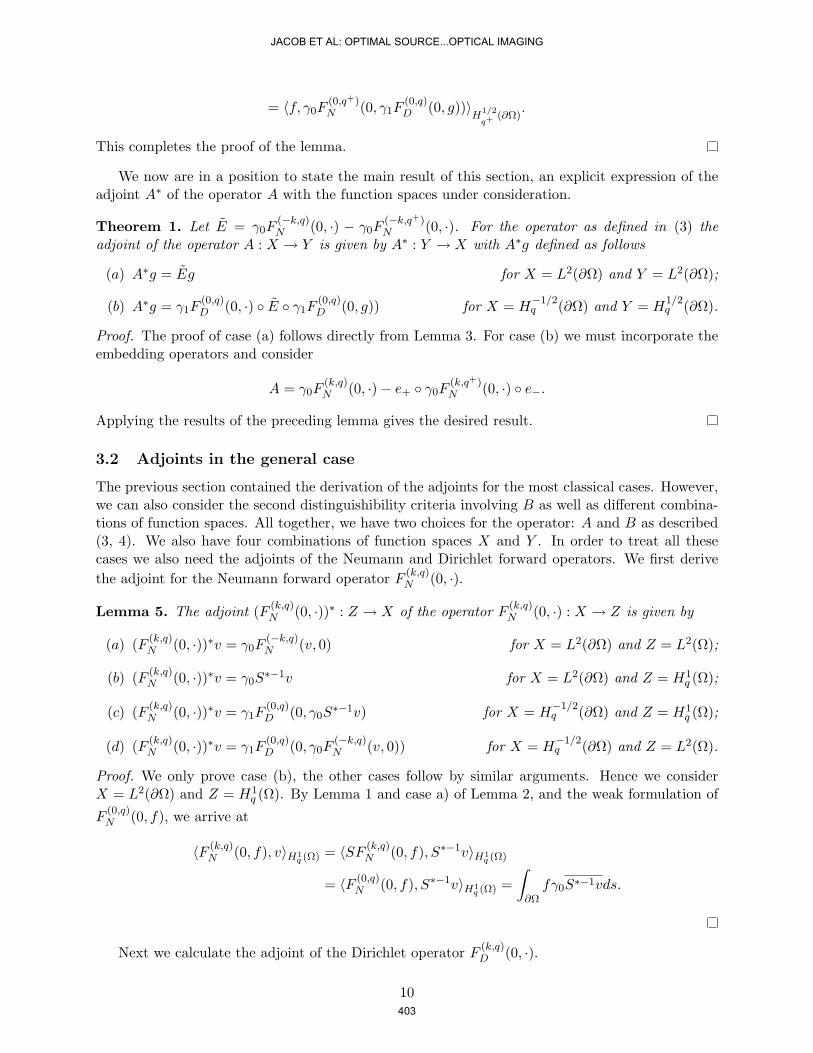
= 〈f, γ0F(0,q+)N (0, γ1F
(0,q)D (0, g))〉
H1/2
q+(∂Ω)
.
This completes the proof of the lemma.
We now are in a position to state the main result of this section, an explicit expression of theadjoint A∗ of the operator A with the function spaces under consideration.
Theorem 1. Let E = γ0F(−k,q)N (0, ·) − γ0F
(−k,q+)N (0, ·). For the operator as defined in (3) the
adjoint of the operator A : X → Y is given by A∗ : Y → X with A∗g defined as follows
(a) A∗g = Eg for X = L2(∂Ω) and Y = L2(∂Ω);
(b) A∗g = γ1F(0,q)D (0, ·) E γ1F
(0,q)D (0, g)) for X = H
−1/2q (∂Ω) and Y = H
1/2q (∂Ω).
Proof. The proof of case (a) follows directly from Lemma 3. For case (b) we must incorporate theembedding operators and consider
A = γ0F(k,q)N (0, ·)− e+ γ0F
(k,q+)N (0, ·) e−.
Applying the results of the preceding lemma gives the desired result.
3.2 Adjoints in the general case
The previous section contained the derivation of the adjoints for the most classical cases. However,we can also consider the second distinguishibility criteria involving B as well as different combina-tions of function spaces. All together, we have two choices for the operator: A and B as described(3, 4). We also have four combinations of function spaces X and Y . In order to treat all thesecases we also need the adjoints of the Neumann and Dirichlet forward operators. We first derivethe adjoint for the Neumann forward operator F (k,q)
N (0, ·).
Lemma 5. The adjoint (F (k,q)N (0, ·))∗ : Z → X of the operator F (k,q)
N (0, ·) : X → Z is given by
(a) (F (k,q)N (0, ·))∗v = γ0F
(−k,q)N (v, 0) for X = L2(∂Ω) and Z = L2(Ω);
(b) (F (k,q)N (0, ·))∗v = γ0S
∗−1v for X = L2(∂Ω) and Z = H1q (Ω);
(c) (F (k,q)N (0, ·))∗v = γ1F
(0,q)D (0, γ0S
∗−1v) for X = H−1/2q (∂Ω) and Z = H1
q (Ω);
(d) (F (k,q)N (0, ·))∗v = γ1F
(0,q)D (0, γ0F
(−k,q)N (v, 0)) for X = H
−1/2q (∂Ω) and Z = L2(Ω).
Proof. We only prove case (b), the other cases follow by similar arguments. Hence we considerX = L2(∂Ω) and Z = H1
q (Ω). By Lemma 1 and case a) of Lemma 2, and the weak formulation of
F(0,q)N (0, f), we arrive at
〈F (k,q)N (0, f), v〉H1
q (Ω) = 〈SF (k,q)N (0, f), S∗−1v〉H1
q (Ω)
= 〈F (0,q)N (0, f), S∗−1v〉H1
q (Ω) =∫∂Ωfγ0S∗−1vds.
Next we calculate the adjoint of the Dirichlet operator F (k,q)D (0, ·).
10
JACOB ET AL: OPTIMAL SOURCE...OPTICAL IMAGING
403
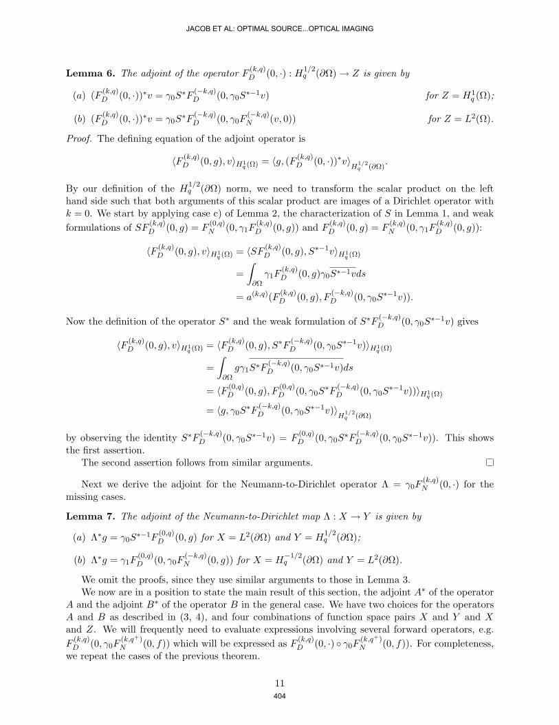
Lemma 6. The adjoint of the operator F (k,q)D (0, ·) : H1/2
q (∂Ω)→ Z is given by
(a) (F (k,q)D (0, ·))∗v = γ0S
∗F(−k,q)D (0, γ0S
∗−1v) for Z = H1q (Ω);
(b) (F (k,q)D (0, ·))∗v = γ0S
∗F(−k,q)D (0, γ0F
(−k,q)N (v, 0)) for Z = L2(Ω).
Proof. The defining equation of the adjoint operator is
〈F (k,q)D (0, g), v〉H1
q (Ω) = 〈g, (F (k,q)D (0, ·))∗v〉
H1/2q (∂Ω)
.
By our definition of the H1/2q (∂Ω) norm, we need to transform the scalar product on the left
hand side such that both arguments of this scalar product are images of a Dirichlet operator withk = 0. We start by applying case c) of Lemma 2, the characterization of S in Lemma 1, and weakformulations of SF (k,q)
D (0, g) = F(0,q)N (0, γ1F
(k,q)D (0, g)) and F
(k,q)D (0, g) = F
(k,q)N (0, γ1F
(k,q)D (0, g)):
〈F (k,q)D (0, g), v〉H1
q (Ω) = 〈SF (k,q)D (0, g), S∗−1v〉H1
q (Ω)
=∫∂Ωγ1F
(k,q)D (0, g)γ0S∗−1vds
= a(k,q)(F (k,q)D (0, g), F (−k,q)
D (0, γ0S∗−1v)).
Now the definition of the operator S∗ and the weak formulation of S∗F (−k,q)D (0, γ0S
∗−1v) gives
〈F (k,q)D (0, g), v〉H1
q (Ω) = 〈F (k,q)D (0, g), S∗F (−k,q)
D (0, γ0S∗−1v)〉H1
q (Ω)
=∫∂Ωgγ1S∗F
(−k,q)D (0, γ0S∗−1v)ds
= 〈F (0,q)D (0, g), F (0,q)
D (0, γ0S∗F
(−k,q)D (0, γ0S
∗−1v))〉H1q (Ω)
= 〈g, γ0S∗F
(−k,q)D (0, γ0S
∗−1v)〉H
1/2q (∂Ω)
by observing the identity S∗F(−k,q)D (0, γ0S
∗−1v) = F(0,q)D (0, γ0S
∗F(−k,q)D (0, γ0S
∗−1v)). This showsthe first assertion.
The second assertion follows from similar arguments.
Next we derive the adjoint for the Neumann-to-Dirichlet operator Λ = γ0F(k,q)N (0, ·) for the
missing cases.
Lemma 7. The adjoint of the Neumann-to-Dirichlet map Λ : X → Y is given by
(a) Λ∗g = γ0S∗−1F
(0,q)D (0, g) for X = L2(∂Ω) and Y = H
1/2q (∂Ω);
(b) Λ∗g = γ1F(0,q)D (0, γ0F
(−k,q)N (0, g)) for X = H
−1/2q (∂Ω) and Y = L2(∂Ω).
We omit the proofs, since they use similar arguments to those in Lemma 3.We now are in a position to state the main result of this section, the adjoint A∗ of the operator
A and the adjoint B∗ of the operator B in the general case. We have two choices for the operatorsA and B as described in (3, 4), and four combinations of function space pairs X and Y and Xand Z. We will frequently need to evaluate expressions involving several forward operators, e.g.F
(k,q)D (0, γ0F
(k,q+)N (0, f)) which will be expressed as F (k,q)
D (0, ·) γ0F(k,q+)N (0, f)). For completeness,
we repeat the cases of the previous theorem.
11
JACOB ET AL: OPTIMAL SOURCE...OPTICAL IMAGING
404

Theorem 2. Let E = γ0F(−k,q)N (0, ·) − γ0F
(−k,q+)N (0, ·). For the operator A as defined in (3), the
adjoint of the operator A : X → Y is given by A∗ : Y → X with A∗g defined as follows
(A1) A∗g = Eg for X = L2(∂Ω) and Y = L2(∂Ω);
(A2) A∗g = E γ1F(0,q)D (0, g) for X = L2(∂Ω) and Y = H
1/2q (∂Ω);
(A3) A∗g = γ1F(0,q)D (0, ·) Eg for X = H
−1/2q (∂Ω) and Y = L2(∂Ω);
(A4) A∗g = γ1F(0,q)D (0, ·) E γ1F
(0,q)D (0, g)) for X = H
−1/2q (∂Ω) and Y = H
1/2q (∂Ω).
Let E = I − γ0F(−k,q+)N (0, ·) γ1F
(−k,q)D (0, ·). For the operator B as defined in (4), the adjoint
of the operator B : X → Z is given by B∗ : Z → X with B∗v defined as follows
(B1) B∗v = E γ0F(−k,q)N (v, 0) for X = L2(∂Ω) and Z = L2(Ω);
(B2) B∗v = E γ0S∗−1v for X = L2(∂Ω) and Z = H1
q (Ω);
(B3) B∗v = γ1F(0,q)D (0, ·) E γ0F
(−k,q)N (v, 0) for X = H
−1/2q (∂Ω) and Z = L2(Ω);
(B4) B∗v = γ1F(0,q)D (0, ·) E γ0S
∗−1v for X = H−1/2q (∂Ω) and Z = H1
q (Ω).
4 Numerical Simulations
In this section, we present numerical results on the optimal sources obtained by maximizing thediscrepancy functionals introduced in (3) and (4) in Section 2. Our computational program is animplementation of the power method on the operator A∗A and B∗B for the cases presented inTheorem 2.
Let us recall the underlying reasoning for computation of the optimal source for maximizingdistinguishability criteria. In a given experiment, the true physical parameters q+ are unknown andwe are given an a priori guess q. The distinguishability criteria test whether q can be distinguishedfrom q+, by searching for a source distribution, which maximizes the “difference” between q+ andq. We use (3) or (4) as a measure for this difference. Further potential applications of such optimalsource designs were discussed in the introduction.
Given the above setup and using different function space configurations we have eight differentmeasures of type (3) or (4). In the following we will present numerical experiments for these casesand develop an ad hoc criterion to select the best optimal source strategy.
4.1 Numerical computation of optimal sources
We use test problems, which consist of a homogeneous background with small inclusions. Thedomain Ω is a disk of radius 4.3 cm with background diffusion coefficient D0 = 5.5 cm−1 andbackground absorption coefficient µ0 = 0.06 cm−1, which are representative values for soft tissues[27, 1]. The value of k is taken to be 108/299792458 cm−1 [1]. Given the background values we havesimulated both single and multiple circular inclusions corresponding to q+ of radius rt centered at(rc, θc). We have used constant background values plus some multiple of the background values asa constant over the inclusion. Given the inclusion q+, we simulated the “synthetic” data. Thenwe chose the background values as a particular guess for q and computed the distinguishabilityoperator both A and B and their adjoints A∗ and B∗ to form A∗A and B∗B for the power iterationto find the optimal source fn at the nth iteration. We have tested the computation of optimal
12
JACOB ET AL: OPTIMAL SOURCE...OPTICAL IMAGING
405
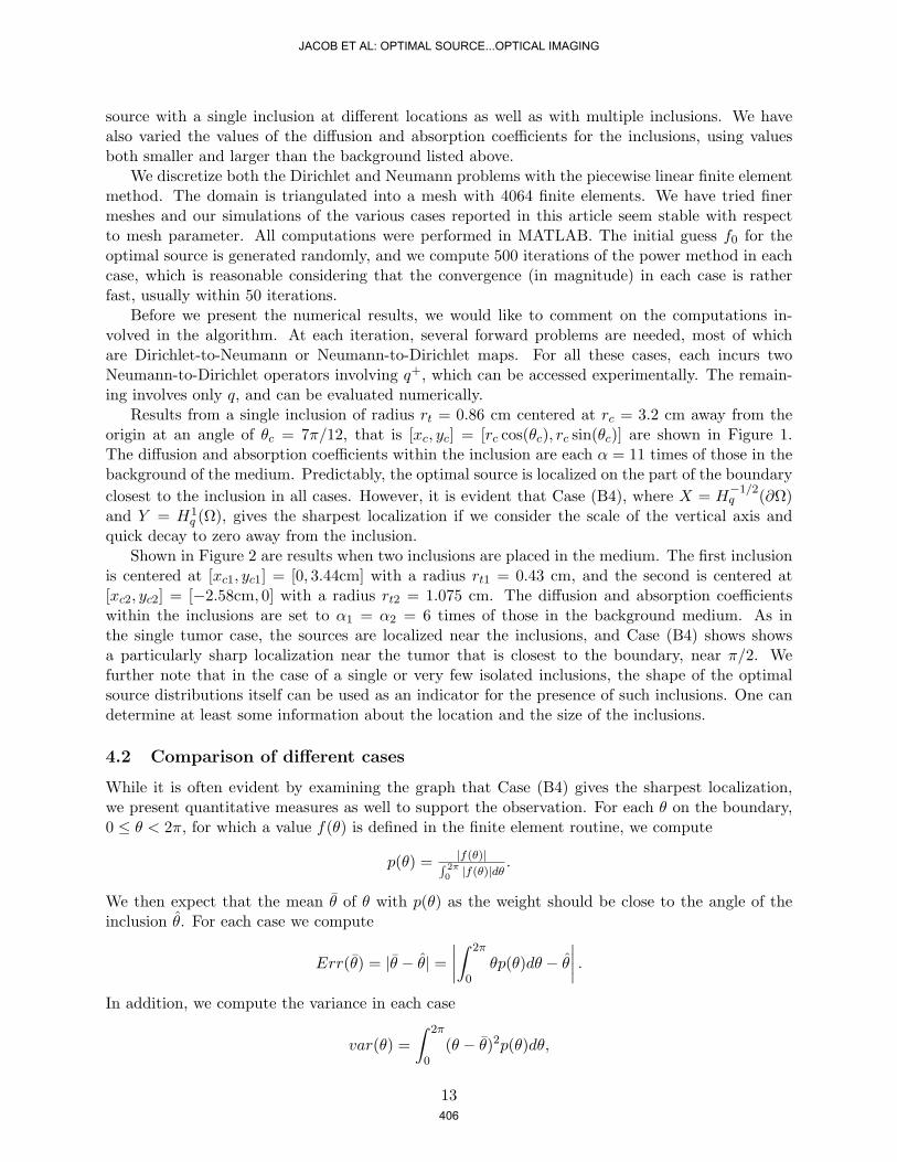
source with a single inclusion at different locations as well as with multiple inclusions. We havealso varied the values of the diffusion and absorption coefficients for the inclusions, using valuesboth smaller and larger than the background listed above.
We discretize both the Dirichlet and Neumann problems with the piecewise linear finite elementmethod. The domain is triangulated into a mesh with 4064 finite elements. We have tried finermeshes and our simulations of the various cases reported in this article seem stable with respectto mesh parameter. All computations were performed in MATLAB. The initial guess f0 for theoptimal source is generated randomly, and we compute 500 iterations of the power method in eachcase, which is reasonable considering that the convergence (in magnitude) in each case is ratherfast, usually within 50 iterations.
Before we present the numerical results, we would like to comment on the computations in-volved in the algorithm. At each iteration, several forward problems are needed, most of whichare Dirichlet-to-Neumann or Neumann-to-Dirichlet maps. For all these cases, each incurs twoNeumann-to-Dirichlet operators involving q+, which can be accessed experimentally. The remain-ing involves only q, and can be evaluated numerically.
Results from a single inclusion of radius rt = 0.86 cm centered at rc = 3.2 cm away from theorigin at an angle of θc = 7π/12, that is [xc, yc] = [rc cos(θc), rc sin(θc)] are shown in Figure 1.The diffusion and absorption coefficients within the inclusion are each α = 11 times of those in thebackground of the medium. Predictably, the optimal source is localized on the part of the boundaryclosest to the inclusion in all cases. However, it is evident that Case (B4), where X = H
−1/2q (∂Ω)
and Y = H1q (Ω), gives the sharpest localization if we consider the scale of the vertical axis and
quick decay to zero away from the inclusion.Shown in Figure 2 are results when two inclusions are placed in the medium. The first inclusion
is centered at [xc1, yc1] = [0, 3.44cm] with a radius rt1 = 0.43 cm, and the second is centered at[xc2, yc2] = [−2.58cm, 0] with a radius rt2 = 1.075 cm. The diffusion and absorption coefficientswithin the inclusions are set to α1 = α2 = 6 times of those in the background medium. As inthe single tumor case, the sources are localized near the inclusions, and Case (B4) shows showsa particularly sharp localization near the tumor that is closest to the boundary, near π/2. Wefurther note that in the case of a single or very few isolated inclusions, the shape of the optimalsource distributions itself can be used as an indicator for the presence of such inclusions. One candetermine at least some information about the location and the size of the inclusions.
4.2 Comparison of different cases
While it is often evident by examining the graph that Case (B4) gives the sharpest localization,we present quantitative measures as well to support the observation. For each θ on the boundary,0 ≤ θ < 2π, for which a value f(θ) is defined in the finite element routine, we compute
p(θ) = |f(θ)|∫ 2π0 |f(θ)|dθ
.
We then expect that the mean θ of θ with p(θ) as the weight should be close to the angle of theinclusion θ. For each case we compute
Err(θ) = |θ − θ| =∣∣∣∣∫ 2π
0θp(θ)dθ − θ
∣∣∣∣ .In addition, we compute the variance in each case
var(θ) =∫ 2π
0(θ − θ)2p(θ)dθ,
13
JACOB ET AL: OPTIMAL SOURCE...OPTICAL IMAGING
406
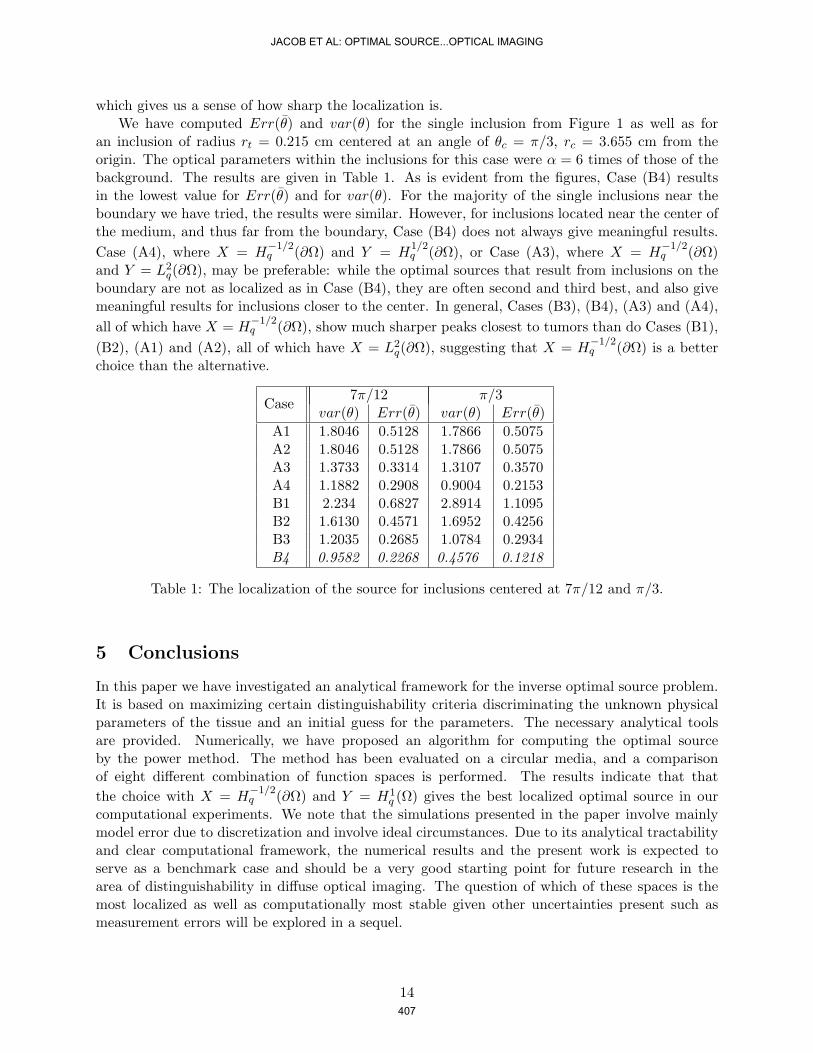
which gives us a sense of how sharp the localization is.We have computed Err(θ) and var(θ) for the single inclusion from Figure 1 as well as for
an inclusion of radius rt = 0.215 cm centered at an angle of θc = π/3, rc = 3.655 cm from theorigin. The optical parameters within the inclusions for this case were α = 6 times of those of thebackground. The results are given in Table 1. As is evident from the figures, Case (B4) resultsin the lowest value for Err(θ) and for var(θ). For the majority of the single inclusions near theboundary we have tried, the results were similar. However, for inclusions located near the center ofthe medium, and thus far from the boundary, Case (B4) does not always give meaningful results.Case (A4), where X = H
−1/2q (∂Ω) and Y = H
1/2q (∂Ω), or Case (A3), where X = H
−1/2q (∂Ω)
and Y = L2q(∂Ω), may be preferable: while the optimal sources that result from inclusions on the
boundary are not as localized as in Case (B4), they are often second and third best, and also givemeaningful results for inclusions closer to the center. In general, Cases (B3), (B4), (A3) and (A4),all of which have X = H
−1/2q (∂Ω), show much sharper peaks closest to tumors than do Cases (B1),
(B2), (A1) and (A2), all of which have X = L2q(∂Ω), suggesting that X = H
−1/2q (∂Ω) is a better
choice than the alternative.
Case7π/12 π/3
var(θ) Err(θ) var(θ) Err(θ)A1 1.8046 0.5128 1.7866 0.5075A2 1.8046 0.5128 1.7866 0.5075A3 1.3733 0.3314 1.3107 0.3570A4 1.1882 0.2908 0.9004 0.2153B1 2.234 0.6827 2.8914 1.1095B2 1.6130 0.4571 1.6952 0.4256B3 1.2035 0.2685 1.0784 0.2934B4 0.9582 0.2268 0.4576 0.1218
Table 1: The localization of the source for inclusions centered at 7π/12 and π/3.
5 Conclusions
In this paper we have investigated an analytical framework for the inverse optimal source problem.It is based on maximizing certain distinguishability criteria discriminating the unknown physicalparameters of the tissue and an initial guess for the parameters. The necessary analytical toolsare provided. Numerically, we have proposed an algorithm for computing the optimal sourceby the power method. The method has been evaluated on a circular media, and a comparisonof eight different combination of function spaces is performed. The results indicate that thatthe choice with X = H
−1/2q (∂Ω) and Y = H1
q (Ω) gives the best localized optimal source in ourcomputational experiments. We note that the simulations presented in the paper involve mainlymodel error due to discretization and involve ideal circumstances. Due to its analytical tractabilityand clear computational framework, the numerical results and the present work is expected toserve as a benchmark case and should be a very good starting point for future research in thearea of distinguishability in diffuse optical imaging. The question of which of these spaces is themost localized as well as computationally most stable given other uncertainties present such asmeasurement errors will be explored in a sequel.
14
JACOB ET AL: OPTIMAL SOURCE...OPTICAL IMAGING
407

Acknowledgments
The second and third authors are partially supported by the Alexander-von-Humboldt Foundation.The third author thanks the National Science Foundation for supporting the work on this projectby grant No. DMS-0915214, and the fourth author thanks the German Science Foundation forsupporting the work on this project by grant MA 1657/18-1.
References
[1] S. R. Arridge. Optical tomography in medical imaging. Inverse Problems, 15(2):R41–R93,1999.
[2] Simon R Arridge and John C Schotland. Optical tomography: forward and inverse problems.Inverse Problems, 25(12):123010 (59pp), 2009.
[3] B. Chance and R. R. Alfano, editors. Photon Migration and Imaging in Random Media andTissues, volume 1888 of (SPIE) Conference Series, September 1993.
[4] B. Chance and R. R. Alfano, editors. Optical Tomography, Photon Migration, and Spectroscopyof Tissue and Model Media: Theory, Human Studies, and Instrumentation, volume 2389 ofSPIE Conference Series, May 1995.
[5] S. Chandrasekhar. Radiative Transfer. Dover, New York, 1960.
[6] M. Cheney and D. Isaacson. Distinguishability in impedance imaging. IEEE Trans. Biomed.Eng., 39(8):852–860, 1992.
[7] Margaret Cheney, David Isaacson, and Jonathan C. Newell. Electrical impedance tomography.SIAM Rev., 41(1):85–101 (electronic), 1999.
[8] John B. Conway. A Course in Functional Analysis, volume 96 of Graduate Texts in Mathe-matics. Springer-Verlag, New York, second edition, 1990.
[9] Alper Corlu, Regine Choe, Turgut Durduran, Kijoon Lee, Martin Schweiger, Simon R. Arridge,Elizabeth M. C. Hillman, and Arjun G. Yodh. Diffuse optical tomography with spectralconstraints and wavelength optimization. Appl. Opt., 44(11):2082–2093, 2005.
[10] D. T. Delpy and M. Cope. Quantification in tissue near-infrared spectroscopy. Phil. Trans. R.Soc. Lond. Ser. B, 352:649–659, June 1997.
[11] Lawrence C. Evans. Partial Differential Equations, volume 19 of Graduate Studies in Mathe-matics. American Mathematical Society, Providence, RI, 1998.
[12] A P Gibson, J C Hebden, and S R Arridge. Recent advances in diffuse optical imaging. Physicsin Medicine and Biology, 50(4):R1–R43, 2005.
[13] D. G. Gisser, D. Isaacson, and J. C. Newell. Electric current computed tomography andeigenvalues. SIAM J. Appl. Math., 50(6):1623–1634, 1990.
[14] Gultekin Gulsen, Bin Xiong, Ozlem Birgul, and Orhan Nalcioglu. Design and implementa-tion of a multifrequency near-infrared diffuse optical tomography system. J. Biomed. Optics,11(1):014020, 2006.
15
JACOB ET AL: OPTIMAL SOURCE...OPTICAL IMAGING
408
[15] Murat Guven, Birsen Yazici, Xavier Intes, and Britton Chance. Diffuse optical tomographywith a priori anatomical information. Physics in Medicine and Biology, 50(12):2837–2858,2005.
[16] Jeremy C Hebden, Simon R Arridge, and David T Delpy. Optical imaging in medicine: I.experimental techniques. Phys. Med. Biol., 42(5):825–840, 1997.
[17] Andreas H Hielscher, Raymond E Alcouffe, and Randall L Barbour. Comparison of finite-difference transport and diffusion calculations for photon migration in homogeneous and het-erogeneous tissues. Phys. Med. Biol., 43(5):1285–1302, 1998.
[18] D. Isaacson. Distinguishability of conductivities by electric current computed tomography.IEEE Trans. Medical Imaging, 5(2):91–95, 1986.
[19] A. Ishimaru. Single Scattering and Transport Theory: Wave Propogation and Scattering inRandom Media I. Academic Press, New York, 1978.
[20] Bangti Jin, Taufiquar Khan, Peter Maass, and Michael Pidcock. Function spaces and optimalcurrents in impedance tomography. Technical report, preprint 17, DFG-Schwerpunktprogramm1324, 2009. http://www.dfg-spp1324.de/download/preprints/preprint017.pdf.
[21] Ian Knowles. A variational algorithm for electrical impedance tomography. Inverse Problems,14(6):1513–1525, 1998.
[22] Ian Knowles. An optimal current functional for electrical impedance tomography. Technicalreport, Department of Mathematics, University of Alabama at Birmingham, 2004. http://www.math.uab.edu/knowles/papers/dnopt.pdf.
[23] Bonnie McAdoo Jacob. Source optimization in abstract function spaces for maximizing distin-guishability: Applications to the optical tomography inverse problem, volume 3402529 of PhDDissertation. Clemson University, Clemson, SC, 2010.
[24] Takefumi Ohta, Norihiko Nishizawa, Tetsuya Ozawa, and Kazuyoshi Itoh. High-speed, high-resolution, and large-scanning-range three-dimensional optical measurement system using awavelength-tunable orthogonally polarized ultrashort twin pulse source. J. Opt. Soc. Am. B,27(1):141–147, 2010.
[25] Guotao Quan, Kun Bi, Shaoqun Zeng, and Qingming Luo. Overcoming ill-posedness of diffuseoptical tomography in steady-state domain. Frontiers of Optoelectronics in China, 1(1):44–49,2008.
[26] Ahmed Serdaroglu, Birsen Yazici, and Kiwoon Kwon. Optimum source design for detection ofheterogeneities in diffuse optical imaging. volume 6139, page 61391A. SPIE, 2006.
[27] Yong Xu, Xuejun Gu, Taufiquar Khan, and Huabei Jiang. Absorption and scattering images ofheterogeneous scattering media can be simultaneously reconstructed by use of dc data. Appl.Opt., 41(25):5427–5437, 2002.
[28] Zhen Yuan, Qizhi Zhang, and Huabei Jiang. Simultaneous reconstruction of acoustic andoptical properties of heterogeneous media by quantitative photoacoustic tomography. Opt.Express, 14(15):6749–6754, 2006.
16
JACOB ET AL: OPTIMAL SOURCE...OPTICAL IMAGING
409

[29] Quing Zhu, Chen Xu, Mark Kane, Yasaman Ardeshirpour, Laura Mariano, Nancy Baccaro,Malini Iyers, Poornima Hegde, Susan Tannenbaum, Scott Kurtzman, and Peter Deckers. Tu-mor angiogenesis of carcinoma in situ, early-stage invasive and larger breast cancers imaged byoptical tomography with ultrasound localization. In Biomedical Optics, page BTuD5. OpticalSociety of America, 2008.
17
JACOB ET AL: OPTIMAL SOURCE...OPTICAL IMAGING
410

(a) Case (A1) (b) Case (A2) (c) Case (A3)
(d) Case (A4) (e) Case (B1) (f) Case (B2)
(g) Case (B3) (h) Case (B4)
Figure 1: Optimal source results from a single inclusion of radius rt = 0.86 cm centered at rc = 3.2cm away from the origin at an angle of θc = 7π/12 are shown. The diffusion and absorptioncoefficients within the inclusion are each α = 11 times of those in the background of the medium.Predictably, the optimal source is localized on the part of the boundary closest to the inclusion inall cases. However, it is evident that Case (B4), where X = H
−1/2q (∂Ω) and Z = H1
q (Ω), gives thesharpest localization if we consider the scale of the vertical axis and quick decay to zero away fromthe inclusion.
18
JACOB ET AL: OPTIMAL SOURCE...OPTICAL IMAGING
411
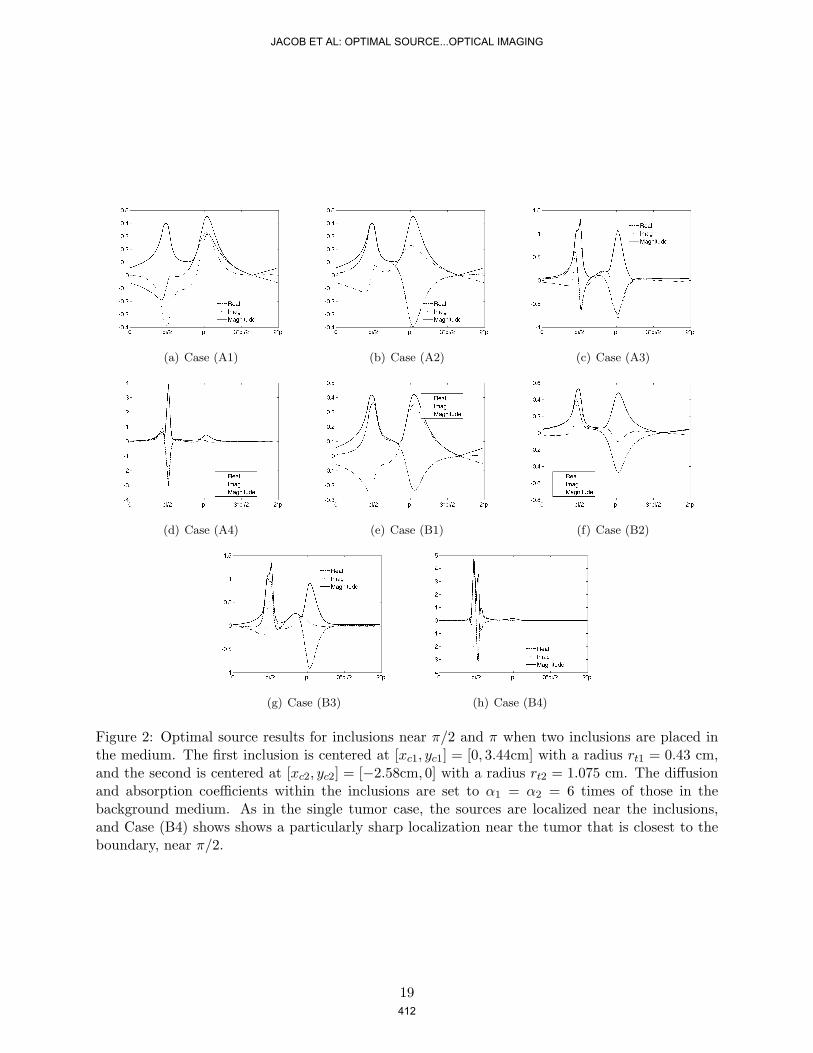
(a) Case (A1) (b) Case (A2) (c) Case (A3)
(d) Case (A4) (e) Case (B1) (f) Case (B2)
(g) Case (B3) (h) Case (B4)
Figure 2: Optimal source results for inclusions near π/2 and π when two inclusions are placed inthe medium. The first inclusion is centered at [xc1, yc1] = [0, 3.44cm] with a radius rt1 = 0.43 cm,and the second is centered at [xc2, yc2] = [−2.58cm, 0] with a radius rt2 = 1.075 cm. The diffusionand absorption coefficients within the inclusions are set to α1 = α2 = 6 times of those in thebackground medium. As in the single tumor case, the sources are localized near the inclusions,and Case (B4) shows shows a particularly sharp localization near the tumor that is closest to theboundary, near π/2.
19
JACOB ET AL: OPTIMAL SOURCE...OPTICAL IMAGING
412

MULTIRESOLUTION ANALYSIS AND HARR-LIKE
WAVELET BASES ON LOCALLY COMPACT GROUPS
Qingde Yang
Department of Mathematics and Statistics, University of Saskatchewan
Saskatoon, SK S7N 5E6 Canada, [email protected]
Keith F. Taylor
Department of Mathematics and Statistics, Dalhousie University
Halifax, NS B3H 3J5 Canada, [email protected]
Abstract. The multiresolution analysis (MRA) on certain non-abelian locally
compact groups G is considered. Characterizations for a refinable function to
generate an MRA in L2(G) are given. Here, no regularity properties or decay
conditions are placed on the scaling functions. MRAs for L2(G) generated by
a self-similar tile as a scaling function are shown and Haar-like wavelet bases
are constructed. Concrete examples related to Heisenberg group are provided
to illustrate the theorems.
Keywords: multiresolution analysis, non-abelian locally compact group,
scaling function, Haar-like wavelet base, Heisenberg group.
1. INTRODUCTION
The theory of wavelets in the Hilbert space L2(Rd) has been studied extensively
in recent decades. The principal framework for constructing and understanding
wavelet bases for the Hilbert space L2(Rd) is the concept of multiresolution analysis
(MRA) [4, 8, 10]. For a general Hilbert space H, the notion of MRA can be
formulated with respect to a distinguished affine structure (Π, σ) in the following
way [1]. Let Π be a countable, discrete subgroup of the group of unitary operators1
413
JOURNAL OF APPLIED FUNCTIONAL ANALYSIS, VOL.7, NO. 4,413-439,COPYRIGHT 2012 EUDOXUS PRESS,LLC
2 MRA ON LOCALLY COMPACT GROUPS
on H and σ be another unitary operator on H satisfying σ−1Πσ⊆Π and 1 < [Π :
σ−1Πσ] < ∞. An MRA with the scaling vector (or function) φ∈H for the affine
structure (Π, σ) is a doubly infinite sequence Vj : j∈Z of closed subspaces of H
with the following properties:
(i) uφ : u∈Π is an orthonormal basis for V0;
(ii) Vj = σjV0, for all j∈Z;
(iii) Vj⊆Vj+1, for all j∈Z;
(iv)⋂
j∈Z Vj = 0 (the triviality of the intersection);
(v)⋃
j∈Z Vj = H (the density of the union).
A scaling vector φ∈H is called refinable if φ∈< σ(uφ) : u∈Π >, the closure
of the finite linear combinations of the functions from < σ(uφ) : u∈Π >. If φ
is refinable, condition (iii) in the above definition is satisfied. Using the unitary
operator σ and the space V0, we get a sequence Vj : j∈Z of nested closed subspaces
of H. In order to construct an MRA, the triviality of the intersection and the
density of the union become two crucial conditions. We will see in section 3 that
the triviality of the intersection is a direct consequence of conditions (i), (ii), and
(iii). The question now is: when does the density of the union hold? To answer
this question, let us first take a look at the Hilbert space L2(Rd).
In L2(Rd), the above mentioned affine structure is Π = Tk : k∈Zd and
σ = σD, where Tx is the translation operator defined by Txf(·) := f(· − x) for any
f∈L2(Rd) and σD is the dilation operator defined by σDf(·) = δ1/2D f(D·) for any
f∈L2(Rd) with D being the dilation matrix and δD = |det(D)|. A special dilation
matrix is D = 2I, where I is the identity matrix. Suppose φ∈L2(Rd). Define
V (φ) as Tkφ : k∈Zd. Then V (φ) is the smallest closed shift invariant subspace
generated by φ, that is, Tkf∈V (φ) for any f∈V (φ) and any k∈Zd. Now define
Vj = σ2IjV (φ) for any j∈Z. The sequence of the closed subspaces Vj : j∈Z
is nested if φ is refinable. A scaling function must be a refinable function. But
the other way around is not true. Boor, DeVore and Ron [2] showed that the
refinability of φ alone is not enough for φ to generate an MRA. For a refinable
function to generate an MRA, additional conditions are required. They proved
414

QINGDE YANG AND KEITH F. TAYLOR 3
that⋃
j∈ZVj = L2(Rd) if and only if φ is refinable and⋃
j∈Zsupp(φj) = Rd modulo
a null-set, where φj(·) := σ2Ijφ(·) = 2dj/2φ(2j ·), φj is the Fourier transform of
φj , and supp(φj) := ξ∈Rd : φj(ξ)6=0 . They also gave a sufficient condition
for the density of the union:⋃
j∈ZVj = L2(Rd) if φ is refinable and φ is nonzero
a.e. in some neighborhood of the origin. This sufficient condition can be easily
proven. If φ is nonzero a.e. in some neighborhood of the origin, then we see that⋃j∈Zsupp(φj) = Rd because φj(·) = φ(·/2j).
In this paper, we are interested in MRA defined over a more abstract Hilbert
space. More specifically, we are interested in MRA defined over Hilbert spaces of the
form L2(G), whereG is some locally compact group. In the case thatG is an abelian
locally compact group, Dahlke has successfully extended the concept of MRA to
L2(G) [3]. The main purpose of this paper is to develop some characterizations
of functions which can serve as scaling functions in the more general case where
the Hilbert space is L2(G), where G is a locally compact group, but may or may
not be abelian. From the abstract harmonic analysis point of view, [2] uses the
information on the Plancherel side to describe the qualities of a refinable function
that can generate an MRA for the space L2(Rd). For a general locally compact
group G, it may be impossible to determine the Plancherel measure on the dual
space G. Thus, the information on the Plancherel side is not available in general
in this case. In contrast to [2], we only use the concepts coming within the space
L2(G) to develop characterizations of functions that can serve as scaling functions
without looking at the Plancherel side. Here, we note that we do not need to
assume that the scaling functions have regularity properties, nor impose any decay
conditions. To make the argument more general, we only assume that the scaling
functions are elements in the space L2(G).
Analogous to the construction of MRA in the space L2(Rd), to build an MRA
on a general group G, the group G must have a uniform lattice subgroup Γ and a
dilative automorphism α such that α(Γ)⊆Γ and 1 < [Γ : α(Γ)] < ∞ (see section
2 for the precise definition). We call (Γ, α) a scaling system. The corresponding
affine structure on L2(G) is then provided by (Π, σα), where Π = λG(Γ), λG is the
415
4 MRA ON LOCALLY COMPACT GROUPS
left regular representation of G, σα is the unitary operator defined by σαf(x) =
δ1/2α f(α(x)) and δα is the factor by which α scales the Haar measure on G.
An important example is G = H, the three dimensional nilpotent Lie group.
H is realized as follows: H = (p, q, t) : p, q, t∈R with group product given by
(p, q, t)(p′, q′, t′) = (p+p′, q+ q′, t+ t′+ 12 (pq′− qp′)). A choice for a uniform lattice
in H is Γ = (m,n, l/2) : m,n, l∈Z and a compatible dilative automorphism is
α(p, q, t) = (2p, 2q, 22t), for all (p, q, t)∈H. This example and variations on it will
be used to illustrate our main results later on.
For any locally compact group G and a subset F⊆L2(G), we say that the family
F is a left zero divisor in L2(G) if there exists a g∈L2(G), g 6=0, such that f∗g = 0,
for all f∈F . If α is an automorphism of G, a single function f∈L2(G) is called
α-substantial if σjαf(·) : j∈Z is not a left zero divisor in L2(G).
If G = R and F⊆L2(G), then F is a left zero divisor in L2(G) if and only
if there exists a measurable subset E of R, of positive Lebesque measure, such
that f(ω) = 0, for all f∈F and almost all ω∈E. If α is the automorphism given
by α(t) = 2t, for all t∈R, then a function f∈L2(R) is α-substantial if and only
if there exists a measurable subset A⊆R such that f(ω)6=0, for almost all ω∈A
and⋃
j∈Z 2jA = R. In the particular case that f(ω)6=0 for almost all ω in a
neighborhood of the origin, then⋃
j∈Z 2jsupp(f) = R. So any such function f is
α-substantial.
Despite the lack of tools from Fourier analysis to help us to recognize α-
substantial functions in the case of a general locally compact group G, we are
able to show that if α is dilative, f∈L2(G), f≥0, f 6=0 and is of compact support,
then f is α-substantial. This is done in section 3.
Consider a locally compact group G. A subspace X of L2(G) is called left shift
invariant if λG(γ)X⊆X, for all γ∈Γ. For φ∈L2(G), let V (φ) denote the smallest
left shift invariant closed subspace of L2(G) containing φ. Define Vj = σjα V (φ),
for all j∈Z. Then the fact that φ is refinable implies that V0⊆V1 (then Vj⊆Vj+1,
for all j∈Z). Define φj(x) = σjαφ(x) = δ
j/2α φ(αj(x)), for any x∈G, j∈Z.
416

QINGDE YANG AND KEITH F. TAYLOR 5
The main results of this paper are summarized in the following theorems.
Theorem 3.1(Triviality of the intersection): Let G be a locally compact group
with a scaling system (Γ, α). Let φ be a refinable function of L2(G) and Vj, j∈Z
defined as above. Suppose that the shifts of φ, that is, Lγφ : γ∈Γ , constitute an
orthonormal basis for V0, then⋂
j∈ZVj = 0.
Theorem 3.5 (Density of the union): Let φ be a refinable function in L2(G)
and Vj, j∈Z defined as above. Then the following are equivalent:
(a)⋃
j∈ZVj = L2(G)
(b) φjj∈Z is a left nonzero divisor in L2(G)
(c) φ is α−substantial.
Theorem 4.3: Let G be a locally compact group and (Γ, α) a scaling system
on G. Suppose that there exists a self-similar tile T for (Γ, α) on G. Then φ = χT
will generate an MRA for the space L2(G).
Theorem 4.6: The MRA generated by a self-similar tile will always guarantee
a Haar-like orthonormal wavelet basis for the space L2(G).
The rest of the paper is arranged as follows. Section 2 provides the basic
concepts, definitions of the terms and some basic results on a scaling system and its
corresponding affine structure. In section 3, we first prove the intersection triviality
theorem. Then we prove several propositions that lead to the proof of theorem 3.5
as stated above. Section 4 concerns with refinable functions of self-similar tile in
the space L2(G), MRAs generated by using these refinable functions as scaling
functions, and Haar-like wavelet bases associated with these MRAs. In section 5,
we turn to the examples of the Heisenberg group. We draw upon the idea of [12]
to give an explicit construction of refinable function on the Heisenberg group. This
construction will provide examples to illustrate our theorems established in sections
3 and 4.
2. BASIC CONCEPTS
Let G be a locally compact group with left Haar measure mG. Integration
with respect to mG will be denoted simply by∫
Gf(x) dx, for any appropriate
417

6 MRA ON LOCALLY COMPACT GROUPS
complex-value function f on G. Let L2(G) denote the Hilbert space of (equivalence
classes of) square integrable complex-valued functions on G with inner product:
< f, g >=∫
Gf(x)g(x) dx, for f, g∈L2(G). The left regular representation of G
is the faithful homomorphism λG of G into the unitary group on L2(G) given by
λG(x)f(y) = f(x−1y), ∀x, y ∈ G, f∈L2(G). If the group of unitary operators on
L2(G) is endowed with the strong operator topology, then λG is continuous. If α is
an automorphism (topological homomorphism and algebraic automorphism) of G,
then f→∫
Gf(α(x)) dx is a left invariant integral so there exists a positive constant
δα so that∫
Gf(x) dx = δα
∫Gf(α(x)) dx, for any appropriate function f onG. This
means that α induces a unitary operator σα on L2(G) by σαf(x) = δ1/2α f(α(x)),
for all x∈G, f∈L2(G). Note that, for any j∈Z, αj is an automorphism of G and
σαjf(x) = δj/2
α f(αj(x)), for all x∈G, f∈L2(G).
An automorphism α of G is called dilative if, for any compact K⊆G and any
neighborhood U of the identity e of G, there exists an n0∈N such that K⊆αn(U),
for all n≥n0. Note that α is dilative implies that δα > 1 but the converse is not
true.
A subgroup Γ of G is called a uniform lattice in G if Γ is discrete, countable
and G/Γ is compact. Suppose Γ is a uniform lattice in G and α is a dilative
automorphism of G such that α(Γ)⊆Γ and 1 < [Γ : α(Γ)] < ∞. Then we will call
(Γ, α) a scaling system (based on G).
For many of the results of this paper, we assume that (Γ, α) is a scaling system.
This condition imposes strong restrictions on the group G and the discrete subgroup
Γ. We will not fully investigate these restrictions here, but we need to make a few
observations.
Proposition 2.1. Let (Γ, α) be a scaling system. Then the following conditions
hold.
(a) G is a unimodular group;
(b) Γ is not an open subgroup of G;
(c) mG(Γ) = 0;
418

QINGDE YANG AND KEITH F. TAYLOR 7
(d) For any j0∈Z,⋃
j≥j0α−j(Γ) is dense in G.
Proof. (a) follows from numbers 1.8 to 1.11 on page 21 in [11] for example.
To see (b), suppose Γ were an open subgroup of G. Then it is a neighborhood
containing the e. Since α(Γ)⊆Γ, if n≥1, then αn(Γ)⊆Γ. Since 1 < [Γ : α(Γ)] and α
is an automorphism of G, Γ is not all of G. Taking U = Γ and K = x for some
x∈G\Γ, then we would have that K = x⊆αn(Γ)⊆Γ by the dilative property of
α, which is a contradiction to the fact that x∈G\Γ. Then (c) follows from (b).
For (d), choose a compact subset K of G such that G =⋃
γ∈ΓKγ; this is
possible because Γ is a uniform lattice in G. For any x∈G and any neighborhood
W of x, let U be a symmetric (U−1 = U) neighborhood of e such that Ux⊆W .
Since α is dilative, there exists n0∈N such that j≥n0 implies K⊆αj(U); that is,
α−j(K)⊆U . Then
G = α−j(G) =⋃γ∈Γ
α−j(Kγ) =⋃γ∈Γ
α−j(K)α−j(γ)⊆⋃γ∈Γ
Uα−j(γ).
Thus, there exists a γ∈Γ such that x∈Uα−j(γ). Hence, x = uα−j(γ), for some u∈U
and α−j(γ) = u−1x∈Ux⊆W . Therefore, W⋂α−j(Γ)6=∅, for any j≥n0. Because
α−j(Γ)⊆α−(j+1)(Γ) for all j,⋃
j≥j0α−j(Γ) is dense in G for any fixed j0∈Z.
If (Γ, α) is a scaling system and φ∈L2(G), we use φ to generate a family of
closed subspaces of L2(G) in analogy with the role played by a scaling vector in an
MRA. Let V (φ) denote the closed linear span of λG(γ)φ : γ∈Γ. For each j∈Z, let
Vj = σαjV (φ). A function of the form λG(γ)φ is called a shift of φ, so the shifts of
φ forms an orthonormal basis exactly when λG(γ)φ : γ∈Γ forms an orthonormal
basis of V (φ). Moreover, the fact that φ is refinable exactly means V0⊆V1. So
Vj⊆Vj+1, for all j∈Z.
Proposition 2.2. Let (Γ, α) be a scaling system and φ∈L2(G). Then the
following conditions hold.
(a) σαjλG(γ)σα
−j = λG(α−j(γ)), for all j∈Z, γ∈Γ,
(b) If Π = λG(Γ), then (Π, σα) is an affine structure on L2(G),
(c) Vj = < λG(ν)σαjφ : ν∈α−j(Γ) >, for j∈Z.
419
8 MRA ON LOCALLY COMPACT GROUPS
Proof. For f∈L2(G) and x∈G, compute
σαjλG(γ)σα
−jf(x) = δj/2α λG(γ)σα
−jf(αj(x)) = δj/2α σα
−jf(γ−1αj(x))
= f(α−j(γ−1)x) = λG(α−j(γ))f(x).
This establishes (a). In particular, σα−1λG(γ)σα = λG(α(γ)). So, if Π = λG(Γ),
then σα−1Πσα = λG(α(Γ)). Since λG is a faithful homomorphism, [Π : σα
−1Πσα] =
[Γ : α(Γ)] and (Π, σα) is an affine structure in the sense of [1]. So (b) holds and (c)
also follows from (a) and the definition of Vj .
3. THE CHARACTERIZATIONS OF A SCALING FUNCTION
In this section, the first two theorems stated in the introduction are proven.
We first prove the triviality of the intersection because it is the direct consequence
of refinability and orthogonal shifts. Then we establish the density of the union by
considering several propositions. Finally, we show that the space L2(G) provides
an abundant supply of α-substantial functions.
Theorem 3.1. (Triviality of the intersection) Let G be a locally compact group
with scaling system (Γ, α). Let φ be a refinable function of L2(G) and define
Vj = σjαV (φ) for j∈Z. Suppose that the shifts of φ, that is, Γγφ : γ∈Γ, constitutes
an orthogonal basis for V0, then⋂
j∈Z Vj = 0.
Proof. Since φ is refinable, Vj⊆Vj+1, for all j∈Z, so⋂j∈Z
Vj =⋂n∈N
V−n.
Since φ is a unit vector with orthogonal shifts and σ is unitary, for each j∈Z,
σj(λG(γ)φ) : γ∈Γ is a orthonormal basis for Vj . The orthogonal projection Pj of
L2(G) onto Vj is given by
Pjf =∑γ∈Γ
< f, σj(λG(γ)φ) > σj(λG(γ)φ), ∀f∈L2(G).
Let f∈⋂
j∈Z Vj ; so Pjf = f , for all j∈Z. Let ε > 0 be arbitrary. Select a
continuous function of compact support, f1, so that ‖f − f1‖2 < ε. Then ‖f −
Pjf1‖2 = ‖Pj(f − f1)‖2 < ε and so ‖f‖2≤‖Pjf1‖2 + ε, for any j∈Z.
420
QINGDE YANG AND KEITH F. TAYLOR 9
Let K be a compact subset of G so that supp(f1)⊆K and let M = sup|f1(x)| :
x∈K. Let W be a neighborhood of e in G such that W⋂
Γ = e. Let U be
another neighborhood of e such that UU−1⊆W . Then, for any γ1, γ2∈Γ, γ1 6=γ2
implies γ−11 U
⋂γ−12 U = ∅.
Since α is dilative, there exists n0∈N such that K⊆αn(U) for any n≥n0; that
is α−n(K)⊆U if n≥n0. Therefore, for γ1, γ2∈Γ, with γ1 6=γ2 and n≥n0, we have
γ−11 α−n(K)
⋂γ−12 α−n(K) = ∅. Let E−n =
⋃γ∈Γ γ
−1α−n(K). If n≥n0, we have
additivity of the characteristic functions,
χE−n =∑γ∈Γ
χγ−1α−n(K).
Now, fix a point x∈G\Γ. Since Γ is discrete in the relative topology of G, it is
a closed subgroup. Thus, there exists a symmetric neighborhood V of e such that
xV⋂
Γ = ∅. Then x is not in γ−1V , for any γ∈Γ. Using the dilative nature of α
again, there exists n1≥n0 such that n≥n1 implies α−n(K)⊆V . So, for any n≥n1,
χE−n(x) = 0. Therefore, the sequence (χE−n
)∞n=1 converges to 0 pointwise on G\Γ,
so it converges to 0 pointwise almost everywhere on G, since mG(Γ) = 0. For n≥n1,
‖P−nf1‖22 =
∑γ∈Γ
| < f1, σ−n(λG(γ)φ) > |2
=∑γ∈Γ
δ−nα |
∫G
f1(x)φ(γ−1α−n(x)) dx|2
≤∑γ∈Γ
δ−nα (
∫G
|f1(x)||φ(γ−1α−n(x))| dx)2
≤ M2∑γ∈Γ
δ−nα (
∫G
|χK(x)||φ(γ−1α−n(x))| dx)2
≤ M2mG(K)2∑γ∈Γ
δ−nα
∫K
|φ(γ−1α−n(x))|2 dx
= M2mG(K)2∑γ∈Γ
∫γ−1α−n(K)
|φ(y)|2 dy
= M2mG(K)2∫
G
χE−n(x)|φ(y)|2 dy−→0, as n→∞,
by the Lebesque Dominated Convergence Theorem. The last inequality in the above
calculation is an application of the Cauch-Schartz inequality. Since ‖f‖2≤‖P−nf1‖2+
421
10 MRA ON LOCALLY COMPACT GROUPS
ε, for all n, ‖f‖2≤ε and ε > 0 being arbitrary, we conclude that f = 0. Therefore,⋂j∈Z Vj = 0.
Remark 3.2. In Theorem 3.1, one can replace the assumption of orthogonal
shifts with the assumption that the shifts of φ constitute a frame in V0, as for
the L2(Rd) situation, but we preferred to write out the clearer argument with the
stronger assumption since we need orthogonal shifts elsewhere.
A subspace X of L2(G) is called left translation invariant if λG(x)f∈X, for all
f∈X and x∈G. For a family of functions F⊆L2(G). Let X(F ) denote the smallest
closed left translation invariant subspace of L2(G) which contains F . Obviously,
X(F ) = < λG(x)f : x∈G, f∈F > = λG(x)f : x∈G, f∈F⊥⊥.
Recall that we call F a left zero divisor in L2(G) if there exists a nonzero g in L2(G)
such that f∗g = 0, for all f∈F .
Proposition 3.3. Let G be a unimodular locally compact group and let F⊆L2(G).
Then X(F ) = L2(G) if and only if F is not a left zero divisor in L2(G).
Proof. For g∈L2(G), let g∗(x) = g(x−1), for all x∈G. Then g−→g∗ is a norm
preserving conjugate linear bijection of L2(G) (this is where unimodularity of G is
used). Now, for f, g∈L2(G) and x∈G, the following is a standard calculation,
f∗g(x) =∫
G
f(y)g(y−1x) dy
=∫
G
f(y)g∗(x−1y) dy
=∫
G
f(xy)g∗(y) dy
= < λG(x−1)f, g∗ > .
Thus, f∗g = 0, for all f∈F if and only if g∗∈λG(z)f : z∈G, f∈F⊥ = X(F )⊥.
Therefore, X(F ) = L2(G) if and only if F is not a left zero divisor in L2(G).
We are most concerned about the nature of X(F ) where F = σαjφ : j∈Z
and φ is a refinable function associated with a scaling system.
422

QINGDE YANG AND KEITH F. TAYLOR 11
Proposition 3.4. Let (Γ, α) be a scaling system and let φ be a refinable func-
tion in L2(G). Then X(σαjφ : j∈Z) =
⋃j∈Z Vj.
Proof. According to Proposition 2.2 (c), for any k∈Z, Vk is generated by
λG(ν)σαkφ : ν∈α−k(Γ). Thus, Vk⊆X(σα
jφ : j∈Z), for all k∈Z. There-
fore,⋃
j∈Z Vj⊆X(σαjφ : j∈Z). Let f∈
⋃j∈Z Vj . Then f∈Vk, for some k, so
λG(ν)f∈Vk, for all ν∈α−k(Γ). But then f∈Vj , for any j≥k, so λG(ν)f∈⋃
j≥k Vj ,
for any ν∈⋃
j≥k α−j(Γ). Because of the nesting properties,
⋃j∈Z Vj is invariant un-
der left translations from⋃
j∈Z α−j(Γ). Therefore,
⋃j∈Z Vj is also invariant under
left translations from⋃
j∈Z α−j(Γ).
Now, for any f∈⋃
j∈Z Vj and any x∈G, use Proposition 2.1 (d) to select a net
(νβ) of elements from⋃
j∈Z α−j(Γ) such that νβ→x in G. Since λG is continu-
ous with respect to the strong operator topology, λG(νβ)f−→λG(x)f . Therefore,
λG(x)f∈⋃
j∈Z Vj , for all x∈G. Hence, X(σαjφ : j∈Z) =
⋃j∈Z Vj .
We are now ready for the main theorem characterizing scaling functions for a
scaling system (Γ, α). Recall that, for φ∈L2(G) and j∈Z, σαjφ(x) = δ
j/2α φ(αj(x))
and φ is α-substantial if and only if σαjφ : j∈Z is not a left zero divisor in L2(G).
Combining Proposition 3.3 and 3.4 gives us that⋃
j∈Z Vj = L2(G) if and only if φ
is refinable and α-substantial. Thus we have the following theorem.
Theorem 3.5. (Density of the union) Let φ be a refinable function in L2(G)
and Vj , j∈Z defined as above. Then the following are equivalent:
(a)⋃
j∈ZVj = L2(G)
(b) φjj∈Z is a left nonzero divisor in L2(G)
(c) φ is α-substantial.
Next we show that the condition of being α-substantial is not really that im-
posing.
Proposition 3.6. Let G be a locally compact group with a dilative automor-
phism α. Let f∈L2(G) satisfy f≥0, f 6=0 and there exists a compact subset K of G
such that f(x) = 0, for almost all x∈G\K. Then f is α-substantial.
423
12 MRA ON LOCALLY COMPACT GROUPS
Proof. Since f is compactly supported, it is actually in L1(G). Without loss
of generality, assume ‖f‖1 = 1. For each n∈N, define fn(x) = δnαf(αn(x)) =
δn/2α σα
nf(x), for all x∈G. Then∫
Gfn(x) dx = 1, for all n∈N. Therefore, for any
g∈L2(G),
fn∗g(y)− g(y) =∫
G
fn(x)[λG(x)g(y)− g(y)]dx,
for all y∈G. Using a version of Minkowski’s inequality for integrals instead of sum,
see [5], VI.11.13 on page 530, we get
‖fn∗g − g‖2 = ∫
G
|fn∗g(y)− g(y)|2dy1/2
= ∫
G
|∫
G
[λG(x)g(y)− g(y)]fn(x) dx|2dy1/2
≤∫
G
∫
G
|λG(x)g(y)− g(y)|2dy1/2fn(x)dx
=∫
G
‖λG(x)g − g‖2fn(x)dx.
For any ε > 0, there exists a neighborhood U of e such that ‖λG(x)g − g‖2 < ε,
for all x∈U (this is just the strong operator continuity of λG again). Since α is
dilative, there exists n0∈N such that α−n(K)⊆U , for all n≥n0. The support of
fn is contained in α−n(K), so n≥n0 and fn(x)6=0 implies ‖λG(x)g − g‖2 < ε, for
almost every x∈G. Therefore, n≥n0 implies
‖fn∗g − g‖2≤∫
G
‖λG(x)g − g‖2fn(x) dx≤ε∫
G
fn(x) dx = ε.
Thus, fn : n = 1, 2, 3, · · · forms a left approximate identity for the module action
of L2(G) on L2(G) by convolution.
Clearly σαnf∗g = 0 implies fn∗g = 0. So σα
nf∗g = 0, for all n∈N implies
g = 0, for all g∈L2(G). Thus, σαjf : j∈Z is not a left zero divisor in L2(G).
That is, f is α-substantial.
4. MRAS GENERATED BY SELF-SIMILAR TILES AND
HAAR-LIKE WAVELET BASES
This section concerns refinable functions that arise from self-similar tiles in
the space L2(G), the MRAs generated by a self-similar tile as its scaling function
424
QINGDE YANG AND KEITH F. TAYLOR 13
and Haar-like wavelet bases associated with the MRAs. Grochenig and Madych
[7] considered the scaling system (Zd, D) on the group Rd, where D is a matrix
with integer entries with all eigenvalues of which have absolute values bigger than
1. They established a connection between self-similar tilings and MRAs that are
generated by a characteristic function for its scaling function. Besides developing
the basic properties of self-similar tiles for (Zd, D), they looked at a variety of
interesting examples by choosing different integer matrices in R2. For example,
the matrix D =
1 −1
1 1
has the fractal set known as the twin dragon as a
self-similar tile. Self-similar tiles are very often fractal in nature. Following Meyer’s
recipe, [7] also constructed Haar-like wavelet bases using the MRAs generated by
self-similar tiles. We have been very much inspired by the results in [7].
Let Γ be a uniform lattice in a locally compact group G. A measurable subset
T of G is called a tile for G if mG(T ) <∞, G =⋃
γ∈Γ γT and mG(γT⋂T ) = 0, for
γ∈Γ\e. Since Γ is countable, the last condition is equivalent to∑
γ∈Γ χT (γ−1x) =
1, for almost all x∈G, where χA denotes the characteristic function of a subset A
of G. The next proposition contains useful observations about tiles.
Proposition 4.1. Let Γ be a uniform lattice in a locally compact group G. Let
T be a tile in G and S a measurable subset of G such that G =⋃
γ∈Γ γS. Then (a)
mG(T ) > 0, (b) S is a tile if and only if mG(S) = mG(T ).
Proof. Since Γ is countable, mG(G) =∑
γ∈ΓmG(T ). So mG(T ) > 0. For
(b), let
f(x) =∑γ∈Γ
χS(γ−1x) =∑γ∈Γ
χγS(x)≥1,
425
14 MRA ON LOCALLY COMPACT GROUPS
for almost all x∈G. Then, for any γ′∈Γ,
mG(T ) =∫
γ′T
1 dx≤∫
γ′T
f(x)dx
=∫
G
χγ′T (x)∑γ∈Γ
χS(γ−1x)dx
=∫
G
∑γ∈Γ
χT (γ′−1γx)χS(x)dx
=∫
G
χS(x)dx = mG(S).
Thus, mG(T )≤mG(S) and mG(T ) = mG(S) if and only if f(x) = 1, for almost all
x∈γ′T , for each γ′∈Γ, so, if and only if S is a tile.
Suppose α is an automorphism of G so that (Γ, α) is a scaling system and T is a
tile for G. If α(T ) =⋃
γ∈Γ0γT , for some subset Γ0⊆Γ, then we call T a self-similar
tile for (Γ, α).
Proposition 4.2. Let (Γ, α) be a scaling system of a locally compact group G.
Suppose that there exists a self-similar tile T for (Γ, α), then the following properties
hold:
(a) If Γ0⊆Γ is such that α(T ) =⋃
γ∈Γ0γT , then Γ0 is a complete set of right
coset representatives for α(Γ) in Γ,
(b) [Γ : α(Γ)] = δα,
(c) φ = mG(T )−1/2χT is a refinable function in L2(G).
Proof. We begin by proving (b). Let γ1,· · · ,γk be a complete set of right coset
representations for α(Γ) in Γ. So Γ is the disjoint union⋃k
i=1 α(Γ)γi.
Since T is a tile for G,
G =⋃γ∈Γ
α(γ)[k⋃
i=1
γiT ].
Applying α−1, we get
G =⋃γ∈Γ
γα−1[k⋃
i=1
γiT ] =⋃γ∈Γ
γ[k⋃
i=1
α−1(γiT )].
426
QINGDE YANG AND KEITH F. TAYLOR 15
If S =⋃k
i=1 α−1(γiT ), then one easily checks thatmG(γS
⋂S) = 0 if γ 6=e. Thus S is
a tile. So mG(S) = mG(T ). On the other hand, mG(S) = kδ−1α mG(T ). Therefore,
[Γ : α(Γ)] = k = δα and (b) holds.
For (a), suppose Γ0 is the subset of Γ such that α(T ) =⋃
γ∈Γ0γT . Then
χα(T )(x) =∑
γ′∈Γ0χγ′T (x), for almost all x. Since G is “tiled” by the sets γT :
γ∈Γ, the χγT : γ∈Γ are mutually orthogonal projections in the commutative von
Newmann algebra L∞(G) (at least, that is a fancy way of thinking for the following
calculation). Each of the following equalities is true for almost every x∈G.
1 =∑γ∈Γ
χγT (x) =∑γ∈Γ
χγT (α−1(x))
=∑γ∈Γ
χα(γ)α(T )(x) =∑
ν∈α(Γ)
χνα(T )(x)
=∑
ν∈α(Γ)
χα(T )(ν−1x) =∑
ν∈α(Γ)
∑γ′∈Γ0
χγ′T (ν−1x)
=∑
ν∈α(Γ)
∑γ′∈Γ0
χ(νγ′)T (x).
Thus,∑
γ∈Γ χγT (x) =∑
ν∈α(Γ)(∑
γ′∈Γ0χ(νγ′)T (x)), for almost every x∈G. This
implies that each γ∈Γ has a unique expression of the form νγ′, with ν∈α(Γ) and
γ′∈Γ0. In other words, Γ0 is a complete set of right coset representations for α(Γ)
in Γ.
Finally, we prove part (c). If φ = mG(T )−1/2χT , then ‖φ‖2 = 1, then φ has
orthogonal shifts and we can see that φ is refinable as follows. For any x∈G,
σ−1α φ(x) = δ−1/2
α φ(α−1(x))
= δ−1/2α mG(T )−1/2χT (α−1(x))
= δ−1/2α mG(T )−1/2χαT (x)
=∑γ∈Γ0
δ−1/2α mG(T )−1/2χγT (x)
=∑γ∈Γ0
δ−1/2α mG(T )−1/2χT (γ−1x)
=∑γ∈Γ0
δ−1/2α λG(γ)φ(x).
427

16 MRA ON LOCALLY COMPACT GROUPS
So σα−1φ =
∑γ∈Γ0
δ−1/2α λG(γ)φ which implies φ =
∑γ∈Γ0
δ−1/2α σα[λG(γ)φ]. There-
fore φ is refinable.
From the proof above, we see that the number of right coset representatives for
α(Γ) in Γ is equal to δα. This number will appear later on.
Boor, DeVore and Ron in [2] showed that refinability is not enough to generate
an MRA in the space L2(Rd). Using the results from section 3, we see that whenever
we have a refinable function of self-similar tile, an MRA can always be produced
by this function as a scaling function in the space L2(G).
Theorem 4.3. Let G be a locally compact group and (Γ, α) a scaling system
on G. Suppose that there exists a self-similar tile T for (Γ, α) on G. Then φ = χT
is a scaling function, that is, it will generate an MRA for the space L2(G).
Proof. The refinability of φ guarantees that condition (iii) in the definition
holds. Define V0 = V (φ), the closure of λG(γ)φ : γ ∈ Γ. It is clear that
λG(γ)φ : γ ∈ Γ is an orthonormal basis for V0. Thus condition (i) holds. Using
the unitary operator σα, a sequence of closed subspaces Vj = σjαV0 are constructed.
Condition (iv) is trivial by Theorem 3.1. By Proposition 3.6, φ is α-substantial.
Thus the density of the union (v) is also satisfied. Therefore, an MRA for L2(G)
is generated by the self-similar tile χT as a scaling function.
Once an MRA has been built up in the space L2(G), next we want to construct
wavelet basis using the structure provided by the MRA.
Let Vj : j∈Z be an MRA in the space L2(G) with a self-similar tile χT
as its scaling function for the scaling system (Γ, α). Let Wj be the orthogonal
complement Vj in Vj+1, that is, Vj+1 = Vj
⊕Wj , j∈Z. Then we can decompose
L2(G) as⊕
j∈Z Wj . To construct an orthogonal wavelet basis for L2(G), all we need
is to construct an orthogonal basis for W0. If an orthogonal basis for W0 can be
constructed, then σjα will send this orthogonal basis for W0 to an orthogonal basis
for Wj , j∈Z. Therefore the union of all these bases would give an orthogonal basis
for L2(G) because L2(G) =⊕
j∈Z Wj . In the space L2(Rd) with a scaling system
428
QINGDE YANG AND KEITH F. TAYLOR 17
(Zd, D), if φ is a scaling function of an MRA and q = |det(D)|, [9] showed that
there exist q − 1 functions ψ1, · · · , ψq−1 such that Tkψi : k∈Zd, i = 1, · · · , q − 1
is an orthogonal basis of W0, where ψi, i = 1, · · · , q − 1 satisfy
(4.1) ψi(x) =∑k∈Zd
aik|det(D)|1/2φ(Dx− k),
with some sequences aik, i = 1, · · · , q − 1 in l2(Zd). Therefore, σjDTkψi :
k∈Zd, j∈Z, i = 1, · · · , q − 1 forms an orthogonal wavelet basis for L2(Rd). Since
V0⊂V1, there must exist a sequence ak in l2(Zd) such that
(4.2) φ(x) =∑k∈Zd
akσDTkφ(x) =∑k∈Zd
ak|det(D)|1/2φ(Dx− k).
To construct a wavelet basis following Meyer’s recipe, one first begins with an MRA
with a scaling function φ satisfying equation (4.2) and then look for wavelet basis
satisfying equation (4.1). For the MRA in L2(Rd) generated by a self-similar tile
as a scaling function, [7] constructed a piecewise constant wavelet basis associated
with the scaling system (Zd, D) following Meyer’s recipe (See [9]). It turns out that
Meyer’s recipe still works in the space L2(G) if an MRA generated by a scaling
function of self-similar tile is available.
Proposition 4.4. Let χT be a self-similar tile associated with a scaling system
(Γ, α) and Vj : j∈Z be an MRA generated by χT . Let Γ0 = γ1, γ2, · · · , γδα be
a complete set of right coset representatives for α(Γ) in Γ. Then the subspace W0
is a set of functions satisfying f(x) =∑
γ∈Γ aγσαλG(γ)χT (x) with aγ in l2(Γ)
satisfying∑
γ′∈Γ0aα(γ)γ′ = 0 for all γ∈Γ.
Proof. A function f∈W0⊂V1 can be written as
f(x) =∑γ∈Γ
aγσαλG(γ)χT (x) =∑γ∈Γ
aγδ1/2α χT (γ−1α(x)),
for some sequence aγ in l2(Γ). A function g∈V0 can be written as
g(x) =∑γ′∈Γ
bγ′λG(γ′)χT (x) =∑γ′∈Γ
bγ′χT (γ′−1x),
429

18 MRA ON LOCALLY COMPACT GROUPS
for some sequence bγ′ in l2(Γ). Then
〈f, g〉 =∫
G
∑γ∈Γ
aγδ1/2α χT (γ−1α(x))
∑γ′∈Γ
bγ′χT (γ′−1x)dx
= δ1/2α
∑γ∈Γ
∑γ′∈Γ
aγbγ′
∫G
χα−1(γT )(x)χγ′T (x)dx
= δ1/2α
∑γ∈Γ
∑γ′∈Γ
aγbγ′mG(α−1(γT )⋂γ′T )
= δ1/2α
∑γ∈Γ
∑γ′∈Γ
aγbγ′mG(α−1(γ)α−1(T )⋂γ′T ).
Since Γ =⋃δα
i=1 α(Γ)γi, which is a union of disjoint right cosets, a sum over the set
Γ is equal to the sum over the set⋃δα
i=1 α(Γ)γi. Thus the above equals
δ1/2α
∑γ∈Γ
∑γ′∈Γ
aγbγ′mG(α−1(γ)α−1(T )⋂γ′T )
= δ1/2α
∑γ∈Γ
δα∑i=1
∑γ′∈Γ
aα(γ)γibγ′mG(α−1(α(γ)γi)α−1(T )
⋂γ′T )
= δ1/2α
∑γ∈Γ
δα∑i=1
∑γ′∈Γ
aα(γ)γibγ′mG(α−1(α(γ)γiT
⋂α(γ′)α(T )))
= δ1/2α
∑γ∈Γ
δα∑i=1
∑γ′∈Γ
aα(γ)γibγ′mG(α−1(α(γ)γiT
⋂α(γ′)
δα⋃j=1
γjT ))
= δ1/2α
∑γ∈Γ
δα∑i=1
∑γ′∈Γ
aα(γ)γibγ′mG(α−1(
δα⋃j=1
(α(γ)γiT⋂α(γ′)γjT )))
= δ1/2α
∑γ∈Γ
δα∑i=1
aα(γ)γibγmG(α−1(α(γ)γiT ))
= δ1/2α
∑γ∈Γ
δα∑i=1
aα(γ)γibγmG(α−1(T ))
= δ1/2α
∑γ∈Γ
cγbγmG(α−1(T )),
where cγ =∑δα
i=1 aα(γ)γi. The third last equality is due to the following basic fact:
mG(α−1(α(γ)γiT⋂α(γ)γjT )) is either equal to 0 or mG(α−1(α(γ)γiT )) because T
is a tile. The second last equality holds because G is unimodular. Thus, 〈f, g〉 =
δ1/2α 〈c, b〉δ−1
α = δ−1/2α 〈c, b〉. Therefore, f∈W0 if and only if f can be written as
f(x) =∑
γ∈Γ aγδ1/2α χT (γ−1α(x)) and cγ =
∑δα
i=1 aα(γ)γi= 0.
430
QINGDE YANG AND KEITH F. TAYLOR 19
Proposition 4.5. Suppose that χT , (Γ, α), Vj : j∈Z, and Γ0 are the same
as in Proposition 4.4. Suppose that U = (uij) is a δα × δα unitary matrix with all
entries on the first row being the same constant δ−1/2α . Then the set of functions
ψ1, ψ2, · · · , ψδ−1 defined by
ψi−1(x) = mG(T )−1/2∑δα
j=1 uijσαλG(γj)χT (x), i = 2, · · · , δα
is a set of mother wavelets for the MRA. That is, the following set
F = λG(γ)ψi : γ∈Γ, i = 1, · · · , δα − 1
is a complete orthonormal basis for the space W0.
Proof. We first show that the set F is an orthogonal system and then prove
it is complete.
In the following, we will use Proposition 2.2 (a): λG(γ)σα = σαλG(α(γ)). For
λG(γ′)ψi−1, λG(γ′′)ψj−1∈F , then
〈λG(γ′)ψi−1, λG(γ′′)ψj−1〉
= 〈λG(γ′)mG(T )−1/2δα∑
m=1
uimσαλG(γm)χT , λG(γ′′)mG(T )−1/2δα∑
n=1
ujnσαλG(γn)χT 〉
= mG(T )−1δα∑
m=1
δα∑n=1
uimujn〈λG(γ′)σαλG(γm)χT , λG(γ′′)σαλG(γn)χT 〉
= mG(T )−1δα∑
m=1
δα∑n=1
uimujn〈λG(γ′)σαλG(γm)χT , λG(γ′′)σαλG(γn)χT 〉
= mG(T )−1δα∑
m=1
δα∑n=1
uimujn〈σαλG(α(γ′))λG(γm)χT , σαλG(α(γ′′))λG(γn)χT 〉
= mG(T )−1δα∑
m=1
δα∑n=1
uimujn〈λG(α(γ′))λG(γm)χT , λG(α(γ′′))λG(γn)χT 〉
= mG(T )−1δα∑
m=1
δα∑n=1
uimujn〈λG(α(γ′)γm)χT , λG(α(γ′′)γn)χT 〉
= mG(T )−1δα∑
m=1
δα∑n=1
uimujnmG(α(γ′)γmT ∩ α(γ′′)γnT )
= mG(T )−1δ(γ′ − γ′′)δα∑
m=1
uimujmmG(T )
= δ(γ′ − γ′′)δ(i− j).
431
20 MRA ON LOCALLY COMPACT GROUPS
Next we show that the set F is complete in W0. For any f∈W0, we want to
prove that if 〈f, λG(γ)ψi−1〉 = 0 for any γ∈Γ, i = 2, 3, · · · , δα, then f = 0. We see
that
〈f, λG(γ)ψi〉 = 〈∑γ′∈Γ
aγ′σαλG(γ′)χT , λG(γ)mG(T )−1/2δα∑
j=1
uijσαλG(γj)χT 〉
= mG(T )−1/2∑γ′∈Γ
δα∑j=1
aγ′uij〈σαλG(γ′)χT , λG(γ)σαλG(γj)χT 〉
= mG(T )−1/2∑γ′∈Γ
δα∑j=1
aγ′uij〈σαλG(γ′)χT , σαλG(α(γ))λG(γj)χT 〉
= mG(T )−1/2∑γ′∈Γ
δα∑j=1
aγ′uij〈λG(γ′)χT , λG(α(γ)γj)χT 〉
= mG(T )−1/2∑γ′∈Γ
δα∑j=1
aγ′uijmG(γ′T⋂α(γ)γjT )
= mG(T )−1/2∑γ′∈Γ
δα∑m=1
δα∑j=1
aα(γ′)γmuijmG(α(γ′)γmT
⋂α(γ)γjT )
= mG(T )−1/2δα∑
m=1
aα(γ)γmuimmG(α(γ)γmT )
= mG(T )1/2δα∑
m=1
aα(γ)γmuim.
Thus, 〈f, λG(γ)ψi−1〉 = 0 for any γ∈Γ, i = 2, 3, · · · , δα means∑δα
m=1 aα(γ)γmuim =
0 for any γ∈Γ, i = 2, 3, · · · , δα. Since f∈W0 and all entries on the first row of the
unitary matrix U = (uij) are constant, proposition 4.4 implies that∑δα
m=1 aα(γ)γmu1m =
0 for any γ∈Γ. Thus,∑δα
m=1 aα(γ)γmuim = 0 for any γ∈Γ, i = 1, 2, 3, · · · , δα. This
shows that, for any γ∈Γ, the vector (aα(γ)γ1 , aα(γ)γ2 , · · · , aα(γ)γδα) is perpendicu-
lar to all rows in the unitary matrix U . So, aα(γ)γmmust be 0 for any γ∈Γ and
m = 1, 2, · · · , δα. Therefore, aγ = 0 for any γ∈Γ. Hence f = 0. That is, The set F
is complete in W0.
Theorem 4.6. Given ψi−1, i = 2, · · · , δα that are defined in Proposition 4.5,
the set σjαψi : j∈Z, i = 1, 2, · · · , δα − 1 forms a complete orthonormal basis for
L2(G).
432

QINGDE YANG AND KEITH F. TAYLOR 21
5. EXAMPLES ON THE HEISENBERG GROUP
The theorems in sections 3 and 4 hold for general space L2(G), where G is
a locally compact group which includes the Heisenberg group as an important
example. In this section, we show examples to illustrate those theorems. All we
need to do is to construct the refinable functions of self-similar tile on the Heisenberg
group. According to the theorems in sections 3 and 4, the existence of refinable
functions of self-similar tile will automatically lead us to build MRAs, hence to
create Haar-like wavelet bases on the Heisenberg group.
Let G be the 2d + 1 dimensional Heisenberg group Hd, which is a nilpotent
Lie group with underlying manifold R2d+1. We denote points in Hd by (q, p, t)
with q, p∈Rd, t∈R, and define the group operation by (q, p, t)(q′, p′, t′) = (q +
q′, p + p′, t + t′ + 12 (p·q′ − p′·q)). Let Γ be the following uniform lattice subgroup
in Hd: Γ = (m,n, l/2) : m, n∈Zd , l∈Z. And let α be a dilative automorphism
given by α(q, p, t) := (2q, 2p, 22t). Then (Γ, α) forms a scaling system on Hd with
δ = [Γ : α(Γ)] = 22(d+1).
It is known (Folland [6]) that every automorphism α of Hd can be uniquely de-
composed as a product of four factors α1α2α3α4, with αj∈Gj (j = 1, 2, 3, 4), where
Gj is defined as follows: G1 denotes the symplectic group ps(d,R); G2 consists of
inner automorphisms: (a, b, c)(q, p, t)(a, b, c)−1 = (q, p, c+ a·p− b·q); G3 consists of
dilations δ[r] defined by δ[r](q, p, t) = (rq, rp, r2t); and G4 consists of two elements,
the identity and the automorphism i defined by i(q, p, t) = (p, q,−t).
We restrict ourself to constructing special self-similar tiles for (Γ, α) on Hd,
where α can be written as α1α3α4. That is, α(q, p, t) = (Dα(q, p), rαt), where rα is
some integer and Dα is a dilative automorphism from R2d to R2d. The fundamental
idea to construct such self-similar tiles for (Γ, α) is the following. We decompose
the process of construction into two steps: first constructing in the direction R2d,
that is, constructing self-similar tiles for the scaling system (Z2d, Dα). The work
in [7] provides us details for this. Then, based on the self-similar tile obtained
for (Z2d, Dα), we construct a self-similar tile in the direction R for (Γ, α). Such
433

22 MRA ON LOCALLY COMPACT GROUPS
a self-similar tile is called a self-similar stacked tile due to the obvious geometric
reason.
For simple notation reason, let’s use (x, t) to denote the element (q, p, t) in
the Heisenberg group, that is, x = (q, p)∈R2d. Then the group law becomes
(x, t)(x′, t′) = (x+x′, t+ t′+S(x, x′)) where S(x, x′) = ((q, p), (q′, p′)) = 1/2(p·q′−
q·p′) is a skew-symmetric bilinear form from R2d×R2d to R.
Let A be a self-similar tile for the scaling system (Z2d, Dα) on R2d. The exis-
tence of A is confirmed by [7]. Such an A is measurable. Without loss of generality,
we can assume that
A⋂
(k+A) = ∅ for k 6=0, k∈Z2d and⋃
k∈Z2d(k+A) = R2d, and Dα(A) =
⋃s
i=1(ki+A)
where k1, k2, · · ·, ks are lattice points that are representatives of distinct cosets
in Z2d/Dα(Z2d). Thus, the Lebesgue measure of A must be 1, see lemma 1 in
[7]. Since the measure of A is 1 and the disjoint union⋃
k∈Z2d(k + A) fill out the
whole space R2d, we could arrange a one to one correspondence between the lattice
points in Z2d and the tiles. Or simply speaking, we can assume that each tile only
contains one lattice point. For x∈R2d, we use [x]A to denote the lattice point that
corresponds to the tile which contains x. Let < x >A=x− [x]A∈A.
Let F be a bounded measurable real-valued function defined first on A and then
extended periodically to the whole space R2d. Thus, we have F (x) = F (< x >A).
We are going to produce a self-similar tile, denoted by T , for the scaling system
(Γ, α) as follows: T = (x, t)∈Hd : x∈A, 0≤t − F (x) < 1/2 , where F is to be
determined later. We can view F (x) as a piece of surface over A and think of T
as a solid over A bounded between two surfaces F (x) and F (x) + 1/2. Thus the
volume of T is equal to 1/2. So we can think of the “thickness” (in the direction
of t-axis) of tile T as 1/2.
For an element γ = (a, l/2)∈Γ, the image of T under the left translation by γ
is given by γT = (x, t)∈Hd : x − a∈A, 0≤t − l/2 − S(a, x − a) − F (x) < 1/2 .
To show that⋃
γ∈ΓγT is a tiling of Hd, we need to check two things. (a)⋃
γ∈ΓγT
is a disjoint union. (b)⋃
γ∈ΓγT fills out the whole space Hd. For (a), if a6=a′, then
434
QINGDE YANG AND KEITH F. TAYLOR 23
(a, l/2)T⋂
(a′, l/2)T = ∅ since the image (a, l/2)T of T is in a stack of tiles lying over
the tile (a, 0)T . If l and l′ are different integers, then (a, l/2)T and (a, l′/2)T are
two different tiles in one stack located at tile (a, 0)T , but (a, l/2)T⋂
(a, l′/2)T = ∅
since the thickness for each tile is 1/2. As for (b), for any (x, t)∈Hd, there exists a
unique element a∈Z2d such that x − a∈A. And also there exists a unique element
l∈Z with the property 0≤t− l/2− S(a, x− a)− F (x− a) < 1/2.
Now, we can start constructing a self-similar stacked tiling related to the tile
A in R2d. From the explanation above, we know that the key point is to determine
the surface described by the equation t = F (x) on A. We start by choosing
Γ0 = (ki, c) : i = 1, 2, · · ·, s, and c = 0, 1/2, 1, 3/2, · · ·, (|rα| − 1)/2 .
Then we have
Proposition 5.1. T is a self-similar stacked tile for (Γ, α) with the above
choice of the finite set Γ0 if and only if the function F (x) on A satisfies
F (x) =1|rα|
F (< Dα(x) >A) +1|rα|
S([Dα(x)]A, < Dα(x) >A).
Proof. By the choice of Γ0, we have⋃γ∈Γ0
γT (disjoint finite union)
= (x, t) : x∈⋃s
i=1(ki +A), 0≤t− S([x]A, < x >A)− F (< x >A) <
|rα|2
= (x, t) : x∈⋃s
i=1(ki +A), 0≤ 1
|rα|t− 1
|rα|S([x]A, < x >A)− 1
|rα|F (< x >A) <
12.
Geometrically speaking, there are s stacks of tiles in⋃
γ∈Γ0γT . For each stack there
are |rα| tiles with the “thickness” for each tile 1/2, so the “thickness” for each stack
is |rα|×1/2. On the other hand,
αT = α (x, t)∈Hd : x∈A, 0≤t− F (x) < 1/2
= (Dα(x), rαt)∈Hd : x∈A, 0≤t− F (x) < 1/2
= (x, t)∈Hd : Dα−1(x)∈A, 0≤ t
|rα|− F (D−1
α (x)) < 1/2
= (x, t)∈Hd : x∈Dα(A) =⋃s
i=1(ki +A) and 0≤ t
|rα|− F (D−1
α (x)) < 1/2 .
435
24 MRA ON LOCALLY COMPACT GROUPS
These two sets are equal if and only if
F (D−1α (x)) =
1|rα|
F (< x >A) +1|rα|
S([x]A, < x >A).
Or equivalently
F (x) =1|rα|
F (< Dα(x) >A) +1|rα|
S([Dα(x)]A, < Dα(x) >A).
This proposition yields the following theorem.
Theorem 5.2. For the choice of Γ0 given above, there exists a unique self-
similar stacked tile T for (Γ, α). The function F (x) is given explicitly by
F (x) =∞∑
m=1
1|rα|m
S([Dmα (x)]Amod (Dα(Z2d)), < Dm
α (x) >A),
where a lattice point k mod (Dα(Z2d)) equals the representative of the coset which
contains element k.
Proof. Define a mapping M from L∞(A) to L∞(A) by
Mf(x) =1|rα|
F (< Dα(x) >A) +1|rα|
S([Dα(x)]Amod (Dα(Z2d)), < Dα(x) >A),
where L∞(A) is a Banach space with the supermum norm. Given f, g∈L∞(A), we
have
‖Mf −Mg‖L∞(A) = ‖ 1|rα|
f(< Dα(x) >A)− 1|rα|
g(< Dα(x) >A)‖L∞(A)
≤ 1|rα|
‖f − g‖L∞(A).
So M is a contractive mapping. There exists a unique fixed point, denoted by F (x).
Especially, we have F = limm→∞Mm0. Thus,
F (x) =∞∑
m=1
1|rm
α |S([Dm
α (x)]Amod (Dα(Z2d)), < Dmα (x) >A).
Now we can provide the first example based on Theorem 5.2.
436

QINGDE YANG AND KEITH F. TAYLOR 25
Example 5.3. Consider α from Hd to Hd defined by α(q, p, t) := (2q, 2p, 22t).
It is clear that α is in G3. We can write α(q, p, t) = (Dα(q, p), rαt) = (2(q, p), 4t).
Thus, rα = 4 and Dα is the dilative automorphism on R2d. Let A = x∈R2d :
0≤xj < 1, j = 1, 2, · · ·, 2n denote the “half open and half closed” standard tile
in the Euclidean space R2d, where xj denotes the jth component of x. Then it is
obvious that⋃
a∈Z2d(A+ a) (disjoint union) fills out the whole space R2d. Clearly,
A is a self-similar tile. If we choose Γ0 = (a, b) : aj = 0 or 1, 1≤j≤2n, b =
0, 1/2, 1 or 3/2 , then by Theorem 5.2, T = (x, t)∈Hd : x∈A, 0≤t−F (x) < 1/2
is a self similar-tile for (Γ, α) with F defined by
F (x) =∞∑
m=1
14m
S([Dmα (x)]Amod (Dm
α (Z2d)), < Dmα (x) >A)
=∞∑
m=1
14m
S([2mx]mod2, < 2mx >),
where [2mx]mod 2 means ([2mx1]mod 2, [2mx2]mod 2, · · · , [2mx2n]mod 2).
Example 5.4. In this example, we choose a different dilative automorphism
on Hd which is defined as follows. α(q, p, t) := (2q, 3p, 6t). This α can be de-
composed as α = α1α3, where α1(q, p, t) := (√
23q,
√32p, t) and α3(q, p, t) :=
(√
6q,√
6p, (√
6)2t) = (√
6q,√
6p, 6t). Further, α can be written as α(q, p, t) =
(Dα(q, p), 6t), where Dα is a dilative automorphism from R2d to R2d defined by
Dα(q, p) := (2q, 3p). Thus, we have rα = 6. Still using the same Γ as the one
used in Example 5.3, we choose Γ0 as the set Γ0 = (a, c), where aj = 0 or 1 for
1≤j≤d, aj = 0, 1 or 2 for d<j≤2d and c = 0, 1/2, 1, · · ·, 5/2. So the set A in
Example 5.3 is a self-similar tile for the scaling system (Z2d, Dα) with dilated tile
by Dα consisting of 6 original tiles. With this self similar tile in R2d, by Theorem
5.2 we obtain a self-similar stacked tile in Hd:
T = (x, t)∈Hd : x∈A, 0≤t− F (x) < 1/2
with F (x) constructed by
F (x) =∞∑
m=1
16m
S([Dαmx]Amod (Dα(Z2d)), < Dα
mx >A),
437
26 MRA ON LOCALLY COMPACT GROUPS
where [Dmα x]Amod (Dα(Z2d)) means [2mx1] mod 2, [2mx2] mod 2, ..., [2mxn] mod
2 and [3mxn+1] mod 3, [3mxn+2] mod 3, ..., [3mx2n] mod 3.
Generally speaking, whenever an automorphism α from H2d to H2d can be
decomposed as α(q, p, t) = (Dα(q, p), rαt) and there exists a self similar tile A in
R2d associated with Dα, then with this A, we can always construct a self similar
tile in Hd associated with α.
The above functions F serve as scaling functions to generate MRAs for the
space L2(Hd). Since F > 0 has compact support, Proposition 3.6 shows that
F is α-substantial. Therefore, F will generate MRAs for L2(Hd) by Theorem
3.5. Theorem 4.6 guarantees the existence of Haar-like wavelet bases for the space
L2(Hd).
6. CONCLUSION
In this paper we are able to give the characterizations for a refinable function
that is capable of generating an MRA in the space L2(G), where G is a locally
compact group that does not have to be abelian. In deriving these characterizations,
we did not use any information from the Plancherel side. In fact, for a general
locally compact group, we may not be able to build the Fourier transform on it.
However, in the case that the Fourier transform can be built up in the space L2(G)
for some non-abelian locally compact groups, how can we characterize a refinable
function to have a scaling function using the information from the Plancherel side?
In particular, if G is a second countable, type I, unimodular locally compact group,
do those results obtained by [2] in the space L2(Rd) mentioned in the introduction
still hold in the space L2(G)? The authors intend to explore these questions in
their future study.
References
[1] L.Baggett, A.Carey, W.Moran and P.Ohring, General existence theorems for orthonormal
wavelets, an abstract approach. Publ.RIMS,Kyoto Univ. 31 (1995), pp.95-111.
[2] C. de Boor, R.Devore, and A.Ron, On the construction of multivariate (pre)wavelets, Con-
str. Approx. 9(1993), pp.123–166.
438
QINGDE YANG AND KEITH F. TAYLOR 27
[3] S.Dahlke, Multiresolution analysis and wavelets on locally compact Abelian groups, in
”Wavelets, Images, and Surface Fitting” (P.J.Laurent, A.Le Mehaute, and L.L.Schumaker,
Eds.), PP.141–156, A.K.Peters, Wellesley, Massachusetts, 1994.
[4] I.Daubechies, Ten lectures on wavelets, CBMF conference series in applied mathematics,
Vol.61, SIAM, Philadelphia,1992.
[5] N.Dunford and J.T.Schwartz, Linear operators, Part I: General theory, Intersience Publish-
ers, New York and London, 1972.
[6] G.B. Folland, Harmonic analysis in phase space, Princeton University Press, Princeton New
Jersey, 1989.
[7] K.Grochenig and W.R.Madych, Multiresolution analysis, Haar bases, and self-similar tilings
of Rn, IEEE Translations on information theory, 38(1992), 556–568.
[8] S.Mallat, Multiresolution approximation and wavelets, Trans.Amer.Math.Soc., 315(1989),
pp.69–88.
[9] Y.Meyer, Ondelettes, functions splines et analyses graduees,,Raport CEREMADE n.8703,
1987.
[10] Y.Meyer, Wavelets and operators, Combridge, Combridge University Press, 1992.
[11] M.S.Raghunathan, Discrete subgroups of Lie groups, Springer Verlag, Berlin, 1972.
[12] R.S.Strichartz, Self-similarity on nilpotent Lie groups, in Contemporary Mathematics,
140(1992), pp.123–157.
439

TABLE OF CONTENTS, JOURNAL OF APPLIED FUNCTIONAL
ANALYSIS, VOL. 7, NO. 4, 2012
Invariant Sets for the Systems of Difference Equations, Iryna Volodymyrivna Komashynska,………………………………………………………………………………..315
Voronovskaya Type Result for q-Derivative of q-Baskakov Operators, Ali Aral and Tuncer Acar,………………………………………………………………………………………….321
Semigroup Algebras and Their Weak Module Amenability, Abasalt Bodaghi,……………..332
The Stability of Solution for a Class of Third Order Nonlinear Vector Differential Equations, Muzaffer Ates,……………………………………………………………………………….339
Square-Mean Almost Periodic Solutions to Some Classes of Nonautonomous Stochastic Evolution Equations with Finite Delay, Paul Bezandry and Toka Diagana,………………...345
Application of Homotopy Analysis Method to Fractional Order Generalized Huxley Equation, K. Hemida and M. S. Mohamed,………………………………………………………………...367
ϵ-Pair proximity in normed spaces, S.A.M. Mohsenalhosseini, H. Mazaheri and M.A. Dehghan……………………………………………………………………………………...373
A Recent Note on the Absolute Riesz Summability Factor of Infinite Series, W. T. Sulaiman,…………………………………………………………………………………….381
On Hilbert's Integral Inequality and Its Applications, W. T. Sulaiman,…………………….388
Optimal Source for Maximum Distinguishability in Optical Imaging, Bonnie Jacob, Bangti Jin, Taufiquar Khan and Peter Maass,…………………………………………………………...394
Multiresolution Analysis and Harr-Like Wavelet Bases on Locally Compact Groups, Qingde Yang and Keith F. Taylor,…………………………………………………………………...413
440