journal of arti cial in telligence researc h 10 (1999) 291...

Journal of Arti�cial Intelligence Research 10 (1999) 291-322 Submitted 10/98; published 5/99

Variational Probabilistic Inference

and the QMR-DT Network

Tommi S. Jaakkola [email protected]

Arti�cial Intelligence Laboratory,

Massachusetts Institute of Technology,

Cambridge, MA 02139 USA

Michael I. Jordan [email protected]

Computer Science Division and Department of Statistics,

University of California,

Berkeley, CA 94720-1776 USA

Abstract

We describe a variational approximation method for e�cient inference in large-scaleprobabilistic models. Variational methods are deterministic procedures that provide ap-proximations to marginal and conditional probabilities of interest. They provide alterna-tives to approximate inference methods based on stochastic sampling or search. We describea variational approach to the problem of diagnostic inference in the \Quick Medical Ref-erence" (QMR) network. The QMR network is a large-scale probabilistic graphical modelbuilt on statistical and expert knowledge. Exact probabilistic inference is infeasible in thismodel for all but a small set of cases. We evaluate our variational inference algorithm on alarge set of diagnostic test cases, comparing the algorithm to a state-of-the-art stochasticsampling method.

1. Introduction

Probabilistic models have become increasingly prevalent in AI in recent years. Beyondthe signi�cant representational advantages of probability theory, including guarantees ofconsistency and a naturalness at combining diverse sources of knowledge (Pearl, 1988),the discovery of general exact inference algorithms has been principally responsible for therapid growth in probabilistic AI (see, e.g., Lauritzen & Spiegelhalter, 1988; Pearl, 1988;Shenoy, 1992). These exact inference methods greatly expand the range of models that canbe treated within the probabilistic framework and provide a unifying perspective on thegeneral problem of probabilistic computation in graphical models.

Probability theory can be viewed as a combinatorial calculus that instructs us in howto merge the probabilities of sets of events into probabilities of composites. The key oper-ation is that of marginalization, which involves summing (or integrating) over the valuesof variables. Exact inference algorithms essentially �nd ways to perform as few sums aspossible during marginalization operations. In terms of the graphical representation ofprobability distributions|in which random variables correspond to nodes and conditionalindependencies are expressed as missing edges between nodes|exact inference algorithmsde�ne a notion of \locality" (for example as cliques in an appropriately de�ned graph), andattempt to restrict summation operators to locally de�ned sets of nodes.

c 1999 AI Access Foundation and Morgan Kaufmann Publishers. All rights reserved.

Jaakkola & Jordan

While this approach manages to stave o� the exponential explosion of exact probabilisticcomputation, such an exponential explosion is inevitable for any calculus that explicitlyperforms summations over sets of nodes. That is, there are models of interest in which\local" is overly large (see Jordan, et al., in press). From this point of view, it is perhapsnot surprising that exact inference is NP-hard (Cooper, 1990).

In this paper we discuss the inference problem for a particular large-scale graphicalmodel, the Quick Medical Reference (QMR) model.1 The QMR model consists of a com-bination of statistical and expert knowledge for approximately 600 signi�cant diseases andapproximately 4000 �ndings. In the probabilistic formulation of the model (the QMR-DT),the diseases and the �ndings are arranged in a bi-partite graph, and the diagnosis problemis to infer a probability distribution for the diseases given a subset of �ndings. Given thateach �nding is generally relevant to a wide variety of diseases, the graph underlying theQMR-DT is dense, re ecting high-order stochastic dependencies. The computational com-plexity of treating these dependencies exactly can be characterized in terms of the size ofthe maximal clique of the \moralized" graph (see, e.g., Dechter, 1998; Lauritzen & Spiegel-halter, 1988). In particular, the running time is exponential in this measure of size. For theQMR-DT, considering the standardized \clinocopathologic conference" (CPC) cases thatwe discuss below, we �nd that the median size of the maximal clique of the moralized graphis 151.5 nodes. This rules out the use of general exact algorithms for the QMR-DT.

The general algorithms do not take advantage of the particular parametric form of theprobability distributions at the nodes of the graph, and it is conceivable that additionalfactorizations might be found that take advantage of the particular choice made by theQMR-DT. Such a factorization was in fact found by Heckerman (1989); his \Quickscorealgorithm" provides an exact inference algorithm that is tailored to the QMR-DT. Unfortu-nately, however, the run time of the algorithm is still exponential in the number of positive�ndings. For the CPC cases, we estimate that the algorithm would require an average of50 years to solve the inference problem on current computers.

Faced with the apparent infeasibility of exact inference for large-scale models such asthe QMR-DT, many researchers have investigated approximation methods. One generalapproach to developing approximate algorithms is to perform exact inference, but to do sopartially. One can consider partial sets of node instantiations, partial sets of hypotheses,and partial sets of nodes. This point of view has led to the development of algorithms forapproximate inference based on heuristic search. Another approach to developing approx-imation algorithms is to exploit averaging phenomena in dense graphs. In particular, lawsof large numbers tell us that sums of random variables can behave simply, converging topredictable numerical results. Thus, there may be no need to perform sums explicitly, eitherexactly or partially. This point of view leads to the variational approach to approximateinference. Finally, yet another approach to approximate inference is based on stochasticsampling. One can sample from simpli�ed distributions and in so doing obtain informationabout a more complex distribution of interest. We discuss each of these methods in turn.

Horvitz, Suermondt and Cooper (1991) have developed a partial evaluation algorithmknown as \bounded conditioning" that works by considering partial sets of node instan-

1. The acronym \QMR-DT" that we use in this paper refers to the \decision-theoretic" reformulation ofthe QMR by Shwe, et al. (1991). Shwe, et al. replaced the heuristic representation employed in theoriginal QMR model (Miller, Fasarie, & Myers, 1986) by a probabilistic representation.

292

Variational Probabilistic Inference and QMR-DT

tiations. The algorithm is based on the notion of a \cutset"; a subset of nodes whoseremoval renders the remaining graph singly-connected. E�cient exact algorithms exist forsingly-connected graphs (Pearl, 1988). Summing over all instantiations of the cutset, onecan calculate posterior probabilities for general graphs using the e�cient algorithm as asubroutine. Unfortunately, however, there are exponentially many such cutset instantia-tions. The bounded conditioning algorithm aims at forestalling this exponential growth byconsidering partial sets of instantiations. Although this algorithm has promise for graphsthat are \nearly singly-connected," it seems unlikely to provide a solution for dense graphssuch as the QMR-DT. In particular, the median cutset size for the QMR-DT across theCPC cases is 106.5, yielding an unmanageably large number of 2106:5 cutset instantiations.

Another approach to approximate inference is provided by \search-based" methods,which consider node instantiations across the entire graph (Cooper, 1985; Henrion, 1991;Peng & Reggia, 1987). The general hope in these methods is that a relatively small fractionof the (exponentially many) node instantiations contains a majority of the probability mass,and that by exploring the high probability instantiations (and bounding the unexploredprobability mass) one can obtain reasonable bounds on posterior probabilities. The QMR-DT search space is huge, containing approximately 2600 disease hypotheses. If, however,one only considers cases with a small number of diseases, and if the hypotheses involvinga small number of diseases contain most of the high probability posteriors, then it maybe possible to search a signi�cant fraction of the relevant portions of the hypothesis space.Henrion (1991) was in fact able to run a search-based algorithm on the QMR-DT inferenceproblem, for a set of cases characterized by a small number of diseases. These were cases,however, for which the exact Quickscore algorithm is e�cient. The more general corpus ofCPC cases that we discuss in the current paper is not characterized by a small number ofdiseases per case. In general, even if we impose the assumption that patients have a limitednumber N of diseases, we cannot assume a priori that the model will show a sharp cuto�in posterior probability after disease N . Finally, in high-dimensional search problems it isoften necessary to allow paths that are not limited to the target hypothesis subspace; inparticular, one would like to be able to arrive at a hypothesis containing few diseases bypruning hypotheses containing additional diseases (Peng & Reggia, 1987). Imposing such alimitation can lead to failure of the search.

More recent partial evaluation methods include the \localized partial evaluation" methodof Draper and Hanks (1994), the \incremental SPI" algorithm of D'Ambrosio (1993), the\probabilistic partial evaluation" method of Poole (1997), and the \mini-buckets" algorithmof Dechter (1997). The former algorithm considers partial sets of nodes, and the latter threeconsider partial evaluations of the sums that emerge during an exact inference run. Theseare all promising methods, but like the other partial evaluation methods it is yet not clear ifthey restrict the exponential growth in complexity in ways that yield realistic accuracy/timetradeo�s in large-scale models such as the QMR-DT.2

Variational methods provide an alternative approach to approximate inference. Theyare similar in spirit to partial evaluation methods (in particular the incremental SPI andmini-buckets algorithms), in that they aim to avoid performing sums over exponentially

2. D'Ambrosio (1994) reports \mixed" results using incremental SPI on the QMR-DT, for a somewhatmore di�cult set of cases than Heckerman (1989) and Henrion (1991), but still with a restricted numberof positive �ndings.

293

Jaakkola & Jordan

many summands, but they come at the problem from a di�erent point of view. From thevariational point of view, a sum can be avoided if it contains a su�cient number of termssuch that a law of large numbers can be invoked. A variational approach to inferencereplaces quantities that can be expected to be the bene�ciary of such an averaging processwith surrogates known as \variational parameters." The inference algorithm manipulatesthese parameters directly in order to �nd a good approximation to a marginal probability ofinterest. The QMR-DT model turns out to be a particularly appealing architecture for thedevelopment of variational methods. As we will show, variational methods have a simplegraphical interpretation in the case of the QMR-DT.

A �nal class of methods for performing approximate inference are the stochastic sam-pling methods. Stochastic sampling is a large family, including techniques such as rejectionsampling, importance sampling, and Markov chain Monte Carlo methods (MacKay, 1998).Many of these methods have been applied to the problem of approximate probabilistic in-ference for graphical models and analytic results are available (Dagum & Horvitz, 1993).In particular, Shwe and Cooper (1991) proposed a stochastic sampling method known as\likelihood-weighted sampling" for the QMR-DT model. Their results are the most promis-ing results to date for inference for the QMR-DT|they were able to produce reasonablyaccurate approximations in reasonable time for two of the di�cult CPC cases. We considerthe Shwe and Cooper algorithm later in this paper; in particular we compare the algorithmempirically to our variational algorithm across the entire corpus of CPC cases.

Although it is important to compare approximation methods, it should be emphasizedat the outset that we do not think that the goal should be to identify a single championapproximate inference technique. Rather, di�erent methods exploit di�erent structuralfeatures of large-scale probability models, and we expect that optimal solutions will involvea combination of methods. We return to this point in the discussion section, where weconsider various promising hybrids of approximate and exact inference algorithms.

The general problem of approximate inference is NP-hard (Dagum & Luby, 1993) andthis provides additional reason to doubt the existence of a single champion approximateinference technique. We think it important to stress, however, that this hardness result,together with Cooper's (1990) hardness result for exact inference cited above, should notbe taken to suggest that exact inference and approximate inference are \equally hard." Totake an example from a related �eld, there exist large domains of solid and uid mechanicsin which exact solutions are infeasible but in which approximate techniques (�nite elementmethods) work well. Similarly, in statistical physics, very few models are exactly solvable,but there exist approximate methods (mean �eld methods, renormalization group methods)that work well in many cases. We feel that the goal of research in probabilistic inferenceshould similarly be that of identifying e�ective approximate techniques that work well inlarge classes of problems.

2. The QMR-DT Network

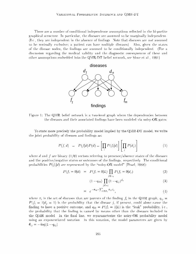
The QMR-DT network (Shwe et al., 1991) is a two-level or bi-partite graphical model (seeFigure 1). The top level of the graph contains nodes for the diseases , and the bottom levelcontains nodes for the �ndings .

294


There are a number of conditional independence assumptions re ected in the bi-partitegraphical structure. In particular, the diseases are assumed to be marginally independent.(I.e., they are independent in the absence of �ndings. Note that diseases are not assumedto be mutually exclusive; a patient can have multiple diseases). Also, given the statesof the disease nodes, the �ndings are assumed to be conditionally independent. (For adiscussion regarding the medical validity and the diagnostic consequences of these andother assumptions embedded into the QMR-DT belief network, see Shwe et al., 1991).

diseases

findings

d1 dn

f1

fm

Figure 1: The QMR belief network is a two-level graph where the dependencies betweenthe diseases and their associated �ndings have been modeled via noisy-OR gates.

To state more precisely the probability model implied by the QMR-DT model, we writethe joint probability of diseases and �ndings as:

P (f; d) = P (f jd)P (d) =

"Yi

P (fijd)

#24Y

j

P (dj)

35 (1)

where d and f are binary (1/0) vectors referring to presence/absence states of the diseasesand the positive/negative states or outcomes of the �ndings, respectively. The conditionalprobabilities P (fijd) are represented by the \noisy-OR model" (Pearl, 1988):

P (fi = 0jd) = P (fi = 0jL)Yj2�i

P (fi = 0jdj) (2)

= (1� qi0)Yj2�i

(1� qij)dj (3)

� e��i0�

Pj2�i

�ijdj ; (4)

where �i is the set of diseases that are parents of the �nding fi in the QMR graph, qij =P (fi = 1jdj = 1) is the probability that the disease j, if present, could alone cause the�nding to have a positive outcome, and qi0 = P (fi = 1jL) is the \leak" probability, i.e.,the probability that the �nding is caused by means other than the diseases included inthe QMR model. In the �nal line, we reparameterize the noisy-OR probability modelusing an exponentiated notation. In this notation, the model parameters are given by�ij = � log(1� qij).

295

Jaakkola & Jordan

3. Inference

Carrying out diagnostic inference in the QMR model involves computing the posteriormarginal probabilities of the diseases given a set of observed positive (fi = 1) and negative(fi0 = 0) �ndings. Note that the set of observed �ndings is considerably smaller than the setof possible �ndings; note moreover (from the bi-partite structure of the QMR-DT graph)that unobserved �ndings have no e�ect on the posterior probabilities for the diseases. Forbrevity we adopt a notation in which f+i corresponds to the event fi = 1, and f�i refersto fi = 0 (positive and negative �ndings respectively). Thus the posterior probabilities ofinterest are P (dj jf

+; f�), where f+ and f� are the vectors of positive and negative �ndings.

The negative �ndings f� are benign with respect to the inference problem|they can beincorporated into the posterior probability in linear time in the number of associated diseasesand in the number of negative �ndings. As we discuss below, this can be seen from thefact that the probability of a negative �nding in Eq. (4) is the exponential of an expressionthat is linear in the dj . The positive �ndings, on the other hand, are more problematic. Inthe worst case the exact calculation of posterior probabilities is exponentially costly in thenumber of positive �ndings (Heckerman, 1989; D'Ambrosio, 1994). Moreover, in practicaldiagnostic situations the number of positive �ndings often exceeds the feasible limit forexact calculations.

Let us consider the inference calculations in more detail. To �nd the posterior probabilityP (djf+; f�), we �rst absorb the evidence from negative �ndings, i.e., we compute P (djf�).This is just P (f�jd)P (d) with normalization. Since both P (f�jd) and P (d) factorize overthe diseases (see Eq. (1) and Eq. (2) above), the posterior P (djf�) must factorize as well.The normalization of P (f�jd)P (d) therefore reduces to independent normalizations overeach disease and can be carried out in time linear in the number of diseases (or negative�ndings). In the remainder of the paper, we concentrate solely on the positive �ndings asthey pose the real computational challenge. Unless otherwise stated, we assume that theprior distribution over the diseases already contains the evidence from the negative �ndings.In other words, we presume that the updates P (dj) P (dj jf

�) have already been made.

We now turn to the question of computing P (dj jf+), the posterior marginal probabilitybased on the positive �ndings. Formally, obtaining such a posterior involves marginalizingP (f+jd)P (d) across the remaining diseases:

P (dj jf+) /

Xdndj

P (f+jd)P (d) (5)

where the summation is over all the possible con�gurations of the disease variables otherthan dj (we use the shorthand summation index d n dj for this). In the QMR modelP (f+jd)P (d) has the form:

P (f+jd)P (d) =

"Yi

P (f+i jd)

#24Yj

P (dj)

35 (6)

=

"Yi

�1� e

��i0�P

j�ijdj

�#24Yj

P (dj)

35 (7)

296


which follows from Eq. (4) and the fact that P (f+i jd) = 1 � P (f�jd). To perform thesummation in Eq. (5) over the diseases, we would have to multiply out the terms 1 � ef�g

corresponding to the conditional probabilities for each positive �nding. The number ofsuch terms is exponential in the number of positive �ndings. While algorithms exist thatattempt to �nd and exploit factorizations in this expression, based on the particular patternof observed evidence (cf. Heckerman, 1989; D'Ambrosio, 1994), these algorithms are limitedto roughly 20 positive �ndings on current computers. It seems unlikely that there is su�cientlatent factorization in the QMR-DT model to be able to handle the full CPC corpus, whichhas a median number of 36 positive �ndings per case and a maximum number of 61 positive�ndings.

4. Variational Methods

Exact inference algorithms perform many millions of arithmetic operations when applied tocomplex graphical models such as the QMR-DT. While this proliferation of terms expressesthe symbolic structure of the model, it does not necessarily express the numeric structureof the model. In particular, many of the sums in the QMR-DT inference problem are sumsover large numbers of random variables. Laws of large numbers suggest that these sumsmay yield predictable numerical results over the ensemble of their summands, and this factmight enable us to avoid performing the sums explicitly.

To exploit the possibility of numerical regularity in dense graphical models we developa variational approach to approximate probabilistic inference. Variational methods are ageneral class of approximation techniques with wide application throughout applied math-ematics. Variational methods are particularly useful when applied to highly-coupled sys-tems. By introducing additional parameters, known as \variational parameters"|whichessentially serve as low-dimensional surrogates for the high-dimensional couplings of thesystem|these methods achieve a decoupling of the system. The mathematical machineryof the variational approach provides algorithms for �nding values of the variational pa-rameters such that the decoupled system is a good approximation to the original coupledsystem.

In the case of probabilistic graphical models variational methods allow us to simplify acomplicated joint distribution such as the one in Eq. (7). This is achieved via parameter-ized transformations of the individual node probabilities. As we will see later, these nodetransformations can be interpreted graphically as delinking the nodes from the graph.

How do we �nd appropriate transformations? The variational methods that we considerhere come from convex analysis (see Appendix 6). Let us begin by considering methods forobtaining upper bounds on probabilities. A well-known fact from convex analysis is thatany concave function can be represented as the solution to a minimization problem:

f(x) = min�f �Tx� f�(�) g (8)

where f�(�) is the conjugate function of f(x). The function f�(�) is itself obtained as thesolution to a minimization problem:

f�(�) = minxf �Tx� f(x) g: (9)

297

Jaakkola & Jordan

The formal identity of this pair of minimization problems expresses the \duality" of f andits conjugate f�.

The representation of f in Eq. (8) is known as a variational transformation. The pa-rameter � is known as a variational parameter. If we relax the minimization and �x the thevariational parameter to an arbitrary value, we obtain an upper bound:

f(x) � �Tx� f�(�): (10)

The bound is better for some values of the variational parameter than for others, and for aparticular value of � the bound is exact.

We also want to obtain lower bounds on conditional probabilities. A straightforwardway to obtain lower bounds is to again appeal to conjugate duality and to express func-tions in terms of a maximization principle. This representation, however, applies to convexfunctions|in the current paper we require lower bounds for concave functions. Our con-cave functions, however, have a special form that allows us to exploit conjugate duality in adi�erent way. In particular, we require bounds for functions of the form f(a+

Pj zj), where

f is a concave function, where zj for i 2 f1; 2; : : : ; ng are non-negative variables, and wherea is a constant. The variables zj in this expression are e�ectively coupled|the impact ofchanging one variable is contingent on the settings of the remaining variables. We can useJensen's inequality, however, to obtain a lower bound in which the variables are decoupled.3

In particular:

f( a+Xj

zj ) = f( a+Xj

qjzjqj

) (11)

�Xj

qj f( a+zjqj

) (12)

where the qj can be viewed as de�ning a probability distribution over the variables zj . Thevariational parameter in this case is the probability distribution q. The optimal settingof this parameter is given by qj = zj=

Pk zk. This is easily veri�ed by substitution into

Eq. (12), and demonstrates that the lower bound is tight.

4.1 Variational Upper and Lower Bounds for Noisy-OR

Let us now return to the problem of computing the posterior probabilities in the QMRmodel. Recall that it is the conditional probabilities corresponding to the positive �ndingsthat need to be simpli�ed. To this end, we write

P (f+i jd) = 1� e��i0�

Pj�ijdj = e log(1�e

�x) (13)

where x = �i0 +P

j �ijdj . Consider the exponent f(x) = log(1 � e�x). For noisy-OR, aswell as for many other conditional models involving compact representations (e.g., logisticregression), the exponent f(x) is a concave function of x. Based on the discussion in the

3. Jensen's inequality, which states that f(a+P

jqjxj) �

Pjqjf(a+ xj), for concave f , where

Pqj = 1,

and 0 � qj � 1, is a simple consequence of Eq. (8), where x is taken to be a+P

jqjxj.

298


previous section, we know that there must exist a variational upper bound for this functionthat is linear in x:

f(x) � �x� f�(�) (14)

Using Eq. (9) to evaluate the conjugate function f�(�) for noisy-OR, we obtain:

f�(�) = �� log � + (� + 1) log(� + 1) (15)

The desired bound is obtained by substituting into Eq. (13) (and recalling the de�nitionx = �i0 +

Pj �ijdj):

P (f+i jd) = ef(�i0+

Pj�ijdj) (16)

� e�i(�i0+

Pj�ijdj)�f�(�i) (17)

� P (f+i jd; �i): (18)

Note that the \variational evidence" P (f+i jd; �i) is the exponential of a term that is linearin the disease vector d. Just as with the negative �ndings, this implies that the variationalevidence can be incorporated into the posterior in time linear in the number of diseasesassociated with the �nding.

There is also a graphical way to understand the e�ect of the transformation. We rewritethe variational evidence as follows:

P (f+i jd; �i) = e�i(�i0+

Pj�ijdj)�f�(�i) (19)

= e �i�i0�f�(�i)

Yj

he �i�ij

idj: (20)

Note that the �rst term is a constant, and note moreover that the product is factorizedacross the diseases. Each of the latter factors can be multiplied with the pre-existingprior on the corresponding disease (possibly itself modulated by factors from the negativeevidence). The constant term can be viewed as associated with a delinked �nding node fi.Indeed, the e�ect of the variational transformation is to delink the �nding node fi from thegraph, altering the priors of the disease nodes that are connected to that �nding node. Thisgraphical perspective will be important for the presentation of our variational algorithm|we will be able to view variational transformations as simplifying the graph until a pointat which exact methods can be run.

We now turn to the lower bounds on the conditional probabilities P (f+i jd). The expo-nent f(�i0 +

Pj �ijdj) in the exponential representation is of the form to which we applied

Jensen's inequality in the previous section. Indeed, since f is concave we need only identifythe non-negative variables zj , which in this case are �ijdj , and the constant a, which is now�i0. Applying the bound in Eq. (12) we have:

P (f+i jd) = ef( �i0+

Pj�ijdj ) (21)

� e

Pjqjjif

��io+

�ijdjqjji

�(22)

299

Jaakkola & Jordan

= e

Pjqjji

hdj f

��io+

�ijqjji

�+(1�dj) f( �io )

i(23)

= e

Pjqjji dj

hf

��io+

�ij

qjji

��f( �io )

i+f( �io )

(24)

� P (f+i jd; q�ji) (25)

where we have allowed a di�erent variational distribution q�ji for each �nding. Note thatonce again the bound is linear in the exponent. As in the case of the upper bound, thisimplies that the variational evidence can be incorporated into the posterior distribution intime linear in the number of diseases. Moreover, we can once again view the variationaltransformation in terms of delinking the �nding node fi from the graph.

4.2 Approximate Inference for QMR

In the previous section we described how variational transformations are derived for indi-vidual �ndings in the QMR model; we now discuss how to utilize these transformations inthe context of an overall inference algorithm.

Conceptually the overall approach is straightforward. Each transformation involvesreplacing an exact conditional probability of a �nding with a lower bound and an upperbound:

P (f+i jd; q�ji) � P (f+i jd) � P (f+i jd; �i): (26)

Given that such transformations can be viewed as delinking the ith �nding node fromthe graph, we see that the transformations not only yield bounds, but also yield a sim-pli�ed graphical structure. We can imagine introducing transformations sequentially untilthe graph is sparse enough that exact methods become feasible. At that point we stopintroducing transformations and run an exact algorithm.

There is a problem with this approach, however. We need to decide at each step whichnode to transform, and this requires an assessment of the e�ect on overall accuracy oftransforming the node. We might imagine calculating the change in a probability of interestboth before and after a given transformation, and choosing to transform that node thatyields the least change to our target probability. Unfortunately we are unable to calculateprobabilities in the original untransformed graph, and thus we are unable to assess the e�ectof transforming any one node. We are unable to get the algorithm started.

Suppose instead that we work backwards. That is, we introduce transformations forall of the �ndings, reducing the graph to an entirely decoupled set of nodes. We optimizethe variational parameters for this fully transformed graph (more on optimization of thevariational parameters below). For this graph inference is trivial. Moreover, it is also easyto calculate the e�ect of reinstating a single exact conditional at one node: we choose toreinstate that node which yields the most change.

Consider in particular the case of the upper bounds (lower bounds are analogous). Eachtransformation introduces an upper bound on a conditional probability P (f+i jd). Thus thelikelihood of observing the (positive) �ndings P (f+) is also upper bounded by its variationalcounterpart P (f+j�):

P (f+) =Xd

P (f+jd)P (d) �Xd

P (f+jd; �)P (d)� P (f+j�) (27)

300


We can assess the accuracy of each variational transformation after introducing and op-timizing the variational transformations for all the positive �ndings. Separately for eachpositive �nding we replace the variationally transformed conditional probability P (f+i jd; �i)with the corresponding exact conditional P (f+i jd) and compute the di�erence between theresulting bounds on the likelihood of the observations:

�i = P (f+j�)� P (f+j� n �i) (28)

where P (f+j� n �i) is computed without transforming the ith positive �nding. The largerthe di�erence �i is, the worse the ith variational transformation is. We should thereforeintroduce the transformations in the ascending order of �is. Put another way, we shouldtreat exactly (not transform) those conditional probabilities whose �i measure is large.

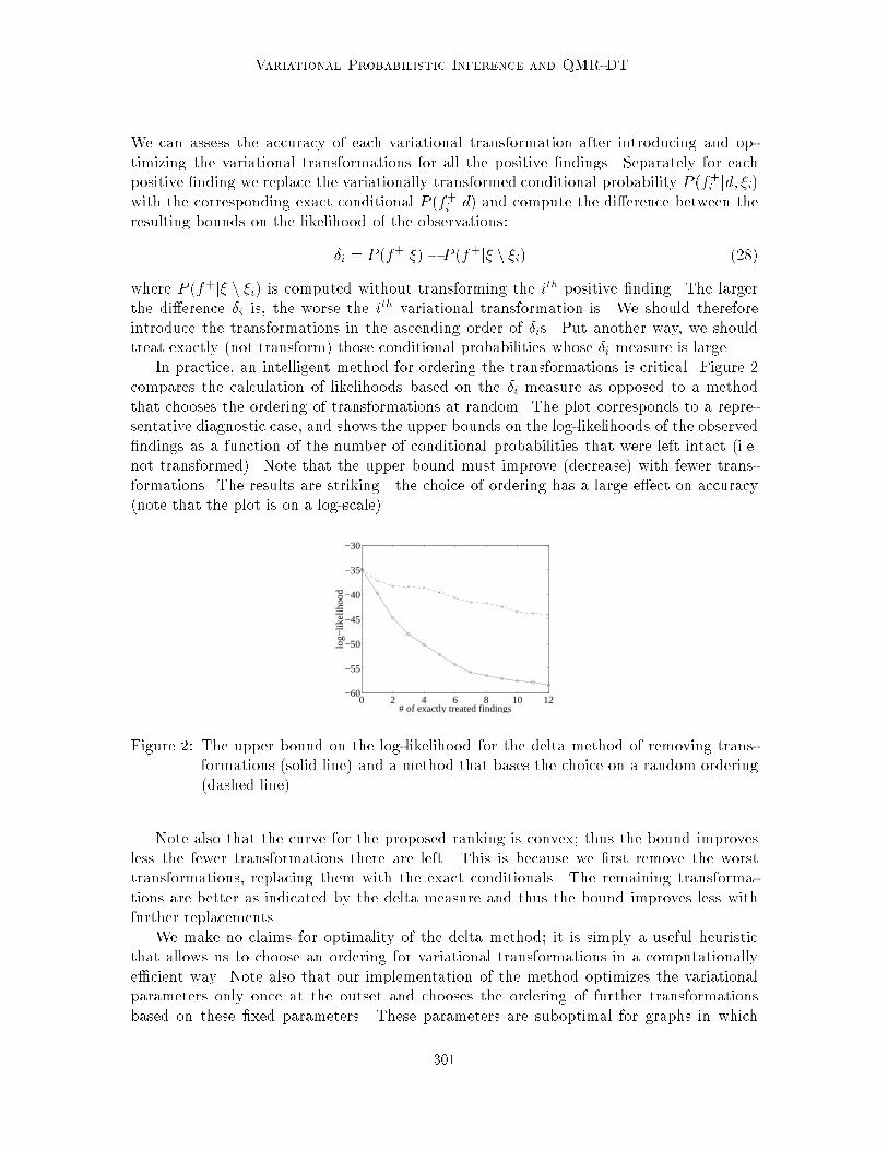
In practice, an intelligent method for ordering the transformations is critical. Figure 2compares the calculation of likelihoods based on the �i measure as opposed to a methodthat chooses the ordering of transformations at random. The plot corresponds to a repre-sentative diagnostic case, and shows the upper bounds on the log-likelihoods of the observed�ndings as a function of the number of conditional probabilities that were left intact (i.e.not transformed). Note that the upper bound must improve (decrease) with fewer trans-formations. The results are striking|the choice of ordering has a large e�ect on accuracy(note that the plot is on a log-scale).

0 2 4 6 8 10 12−60

−55

−50

−45

−40

−35

−30

# of exactly treated findings

log−

likel

ihoo

d

Figure 2: The upper bound on the log-likelihood for the delta method of removing trans-formations (solid line) and a method that bases the choice on a random ordering(dashed line).

Note also that the curve for the proposed ranking is convex; thus the bound improvesless the fewer transformations there are left. This is because we �rst remove the worsttransformations, replacing them with the exact conditionals. The remaining transforma-tions are better as indicated by the delta measure and thus the bound improves less withfurther replacements.

We make no claims for optimality of the delta method; it is simply a useful heuristicthat allows us to choose an ordering for variational transformations in a computationallye�cient way. Note also that our implementation of the method optimizes the variationalparameters only once at the outset and chooses the ordering of further transformationsbased on these �xed parameters. These parameters are suboptimal for graphs in which

301

Jaakkola & Jordan

substantial numbers of nodes have been reinstated, but we have found in practice that thissimpli�ed algorithm still produces reasonable orderings.

Once we have decided which nodes to reinstate, the approximate inference algorithmcan be run. We introduce transformations at those nodes that were left transformed by theordering algorithm. The product of all of the exact conditional probabilities in the graphwith the transformed conditional probabilities yields an upper or lower bound on the overalljoint probability associated with the graph (the product of bounds is a bound). Sums ofbounds are still bounds, and thus the likelihood (the marginal probability of the �ndings)is bounded by summing across the bounds on the joint probability. In particular, an upperbound on the likelihood is obtained via:

P (f+) =Xd

P (f+jd)P (d) �Xd

P (f+jd; �)P (d)� P (f+j�) (29)

and the corresponding lower bound on the likelihood is obtained similarly:

P (f+) =Xd

P (f+jd)P (d) �Xd

P (f+jd; q)P (d)� P (f+jq) (30)

In both cases we assume that the graph has been su�ciently simpli�ed by the variationaltransformations so that the sums can be performed e�ciently.

The expressions in Eq. (29) and Eq. (30) yield upper and lower bounds for arbitraryvalues of the variational parameters � and q. We wish to obtain the tightest possible bounds,thus we optimize these expressions with respect to � and q. We minimize with respect to� and maximize with respect to q. Appendix 6 discusses these optimization problems indetail. It turns out that the upper bound is convex in the � and thus the adjustment of thevariational parameters for the upper bound reduces to a convex optimization problem thatcan be carried out e�ciently and reliably (there are no local minima). For the lower boundit turns out that the maximization can be carried out via the EM algorithm.

Finally, although bounds on the likelihood are useful, our ultimate goal is to approximatethe marginal posterior probabilities P (dj jf+). There are two basic approaches to utilizingthe variational bounds in Eq. (29) and Eq. (30) for this purpose. The �rst method, which willbe our emphasis in the current paper, involves using the transformed probability model (themodel based either on upper or lower bounds) as a computationally e�cient surrogate for theoriginal probability model. That is, we tune the variational parameters of the transformedmodel by requiring that the model give the tightest possible bound on the likelihood. Wethen use the tuned transformed model as an inference engine to provide approximations toother probabilities of interest, in particular the marginal posterior probabilities P (dj jf+).The approximations found in this manner are not bounds, but are computationally e�cientapproximations. We provide empirical data in the following section that show that thisapproach indeed yields good approximations to the marginal posteriors for the QMR-DTnetwork.

A more ambitious goal is to obtain interval bounds for the marginal posterior probabil-ities themselves. To this end, let P (f+; djj�) denote the combined event that the QMR-DTmodel generates the observed �ndings f+ and that the jth disease takes the value dj . Thesebounds follow directly from:

P (f+; dj) =Xdndj

P (f+jd)P (d) �Xdndj

P (f+jd; �)P (d)� P (f+; djj�) (31)

302


where P (f+jd; �) is a product of upper-bound transformed conditional probabilities andexact (untransformed) conditionals. Analogously we can compute a lower bound P (f+; djjq)by applying the lower bound transformations:

P (f+; dj) =Xdndj

P (f+jd)P (d) �Xdndj

P (f+jd; q)P (d)� P (f+; djjq) (32)

Combining these bounds we can obtain interval bounds on the posterior marginal proba-bilities for the diseases (cf. Draper & Hanks 1994):

P (f+; djjq)

P (f+; �dj j�) + P (f+; djjq)� P (dj jf

+) �P (f+; dj j�)

P (f+; djj�) + P (f+; �dj jq); (33)

where �dj is the binary complement of dj .

5. Experimental Evaluation

The diagnostic cases that we used in evaluating the performance of the variational tech-niques were cases abstracted from clinocopathologic conference (\CPC") cases. These casesgenerally involve multiple diseases and are considered to be clinically di�cult cases. Theyare the cases in which Middleton et al. (1990) did not �nd their importance sampling methodto work satisfactorily.

Our evaluation of the variational methodology consists of three parts. In the �rst partwe exploit the fact that for a subset of the CPC cases (4 of the 48 cases) there are asu�ciently small number of positive �ndings that we can calculate exact values of theposterior marginals using the Quickscore algorithm. That is, for these four cases we wereable to obtain a \gold standard" for comparison. We provide an assessment of the accuracyand e�ciency of variational methods on those four CPC cases. We present variationalupper and lower bounds on the likelihood as well as scatterplots that compare variationalapproximations of the posterior marginals to the exact values. We also present comparisonswith the likelihood-weighted sampler of Shwe and Cooper (1991).

In the second section we present results for the remaining, intractable CPC cases. Weuse lengthy runs of the Shwe and Cooper sampling algorithm to provide a surrogate for thegold standard in these cases.

Finally, in the third section we consider the problem of obtaining interval bounds onthe posterior marginals.

5.1 Comparison to Exact Marginals

Four of the CPC cases have 20 or fewer positive �ndings (see Table 1), and for these casesit is possible to calculate the exact values of the likelihood and the posterior marginalsin a reasonable amount of time. We used Heckerman's \Quickscore" algorithm (Hecker-man 1989)|an algorithm tailored to the QMR-DT architecture|to perform these exactcalculations.

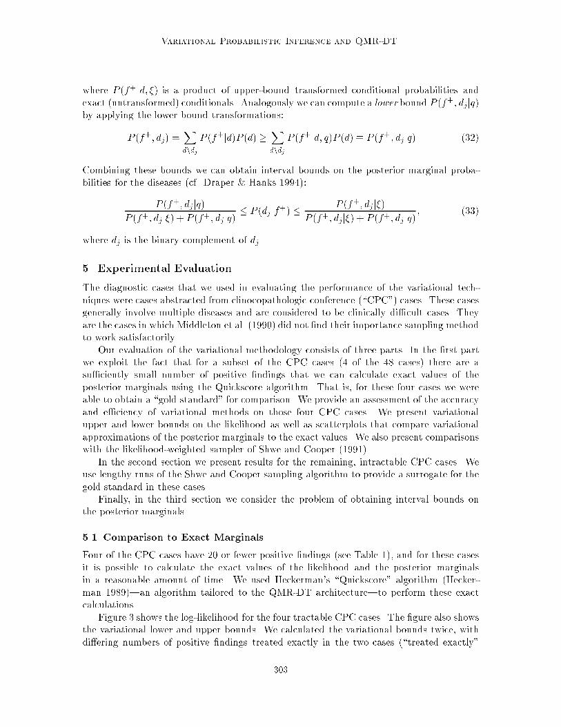
Figure 3 shows the log-likelihood for the four tractable CPC cases. The �gure also showsthe variational lower and upper bounds. We calculated the variational bounds twice, withdi�ering numbers of positive �ndings treated exactly in the two cases (\treated exactly"

303

Jaakkola & Jordan

case # of pos. �ndings # of neg. �ndings

1 20 14

2 10 21

3 19 19

4 19 33

Table 1: Description of the cases for which we evaluated the exact posterior marginals.

(a)0 1 2 3 4 5

−70

−60

−50

−40

−30

−20

sorted cases

log−

likel

ihoo

d

(b)0 1 2 3 4 5

−70

−60

−50

−40

−30

−20

sorted cases

log−

likel

ihoo

d

Figure 3: Exact values and variational upper and lower bounds on the log-likelihoodlogP (f+j�) for the four tractable CPC cases. In (a) 8 positive �ndings weretreated exactly, and in (b) 12 positive �ndings were treated exactly.

simply means that the �nding is not transformed variationally). In panel (a) there were 8positive �ndings treated exactly, and in (b) 12 positive �ndings were treated exactly. Asexpected, the bounds were tighter when more positive �ndings were treated exactly.4

The average running time across the four tractable CPC cases was 26.9 seconds forthe exact method, 0.11 seconds for the variational method with 8 positive �ndings treatedexactly, and 0.85 seconds for the variational method with 12 positive �ndings treated exactly.(These results were obtained on a 433 MHz DEC Alpha computer).

Although the likelihood is an important quantity to approximate (particularly in appli-cations in which parameters need to be estimated), of more interest in the QMR-DT settingare the posterior marginal probabilities for the individual diseases. As we discussed in theprevious section, the simplest approach to obtaining variational estimates of these quan-tities is to de�ne an approximate variational distribution based either on the distributionP (f+j�), which upper-bounds the likelihood, or the distribution P (f+jq), which lower-bounds the likelihood. For �xed values of the variational parameters (chosen to providea tight bound to the likelihood), both distributions provide partially factorized approxi-mations to the joint probability distribution. These factorized forms can be exploited as

4. Given that a signi�cant fraction of the positive �ndings are being treated exactly in these simulations, onemay wonder what if any additional accuracy is due to the variational transformations. We address thisconcern later in this section and demonstrate that the variational transformations are in fact responsiblefor a signi�cant portion of the accuracy in these cases.

304


e�cient approximate inference engines for general posterior probabilities, and in particularwe can use them to provide approximations to the posterior marginals of individual diseases.

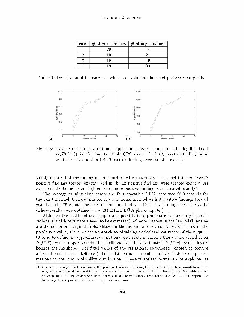
In practice we found that the distribution P (f+j�) yielded more accurate posteriormarginals than the distribution P (f+jq), and we restrict our presentation to P (f+j�). Fig-ure 4 displays a scatterplot of these approximate posterior marginals, with panel (a) corre-

(a)0 0.2 0.4 0.6 0.8 1

0

0.2

0.4

0.6

0.8

1

exact marginals

varia

tiona

l est

imat

es

(b)0 0.2 0.4 0.6 0.8 1

0

0.2

0.4

0.6

0.8

1

exact marginals

varia

tiona

l est

imat

esFigure 4: Scatterplot of the variational posterior estimates and the exact marginals. In

(a) 8 positive �ndings were treated exactly and in (b) 12 positive �ndings weretreated exactly.

sponding to the case in which 8 positive �ndings were treated exactly and panel (b) the casein which 12 positive �ndings treated exactly. The plots were obtained by �rst extractingthe 50 highest posterior marginals from each case using exact methods and then computingthe approximate posterior marginals for the corresponding diseases. If the approximatemarginals are in fact correct then the points in the �gures should align along the diagonalsas shown by the dotted lines. We see a reasonably good correspondence|the variationalalgorithm appears to provide a good approximation to the largest posterior marginals. (Wequantify this correspondence with a ranking measure later in this section).

A current state-of-the-art algorithm for the QMR-DT is the enhanced version of likelihood-weighted sampling proposed by Shwe and Cooper (1991). Likelihood-weighted sampling isa stochastic sampling method proposed by Fung and Chang (1990) and Shachter and Peot(1990). Likelihood-weighted sampling is basically a simple forward sampling method thatweights samples by their likelihoods. It can be enhanced and improved by utilizing \self-importance sampling" (see Shachter & Peot, 1990), a version of importance sampling inwhich the importance sampling distribution is continually updated to re ect the currentestimated posterior distribution. Middleton et al. (1990) utilized likelihood-weighted sam-pling with self-importance sampling (as well as a heuristic initialization scheme known as\iterative tabular Bayes") for the QMR-DT model and found that it did not work sat-isfactorily. Subsequent work by Shwe and Cooper (1991), however, used an additionalenhancement to the algorithm known as `Markov blanket scoring" (see Shachter & Peot,1990), which distributes fractions of samples to the positive and negative values of a nodein proportion to the probability of these values conditioned on the Markov blanket of thenode. The combination of Markov blanket scoring and self-importance sampling yielded

305

Jaakkola & Jordan

an e�ective algorithm.5 In particular, with these modi�cations in place, Shwe and Cooperreported reasonable accuracy for two of the di�cult CPC cases.

We re-implemented the likelihood-weighted sampling algorithm of Shwe and Cooper,incorporating the Markov blanket scoring heuristic and self-importance sampling. (We didnot utilize \iterative tabular Bayes" but instead utilized a related initialization scheme{\heuristic tabular Bayes"{also discussed by Shwe and Cooper). In this section we discussthe results of running this algorithm on the four tractable CPC cases, comparing to theresults of variational inference.6 In the following section we present a fuller comparativeanalysis of the two algorithms for all of the CPC cases.

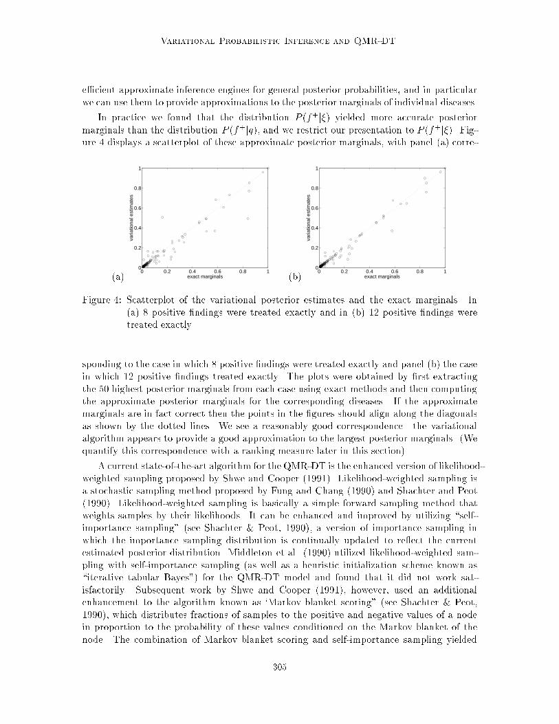
Likelihood-weighting sampling, and indeed any sampling algorithm, realizes a time-accuracy tradeo�|taking additional samples requires more time but improves accuracy.In comparing the sampling algorithm to the variational algorithm, we ran the samplingalgorithm for several di�erent total time periods, so that the accuracy achieved by thesampling algorithm roughly covered the range achieved by the variational algorithm. Theresults are shown in Figure 5, with the right-hand curve corresponding to the sampling runs.The �gure displays the mean correlations between the approximate and exact posteriormarginals across ten independent runs of the algorithm (for the four tractable CPC cases).

10−1

100

101

102

0.86

0.88

0.9

0.92

0.94

0.96

0.98

1

execution time in seconds

mea

n co

rrel

atio

n

Figure 5: The mean correlation between the approximate and exact posterior marginals asa function of the execution time (in seconds). Solid line: variational estimates;dashed line: likelihood-weighting sampling. The lines above and below the sam-pling result represent standard errors of the mean based on the ten independentruns of the sampler.

Variational algorithms are also characterized by a time-accuracy tradeo�. In particular,the accuracy of the method generally improves as more �ndings are treated exactly, atthe cost of additional computation. Figure 5 also shows the results from the variationalalgorithm (the left-hand curve). The three points on the curve correspond to up to 8, 12 and

5. The initialization method proved to have little e�ect on the inference results.6. We also investigated Gibbs sampling (Pearl, 1988). The results from Gibbs sampling were not as good

as the results from likelihood-weighted sampling, and we report only the latter results in the remainderof the paper.

306


16 positive �ndings treated exactly. Note that the variational estimates are deterministicand thus only a single run was made.

The �gure shows that to achieve roughly equivalent levels of accuracy, the samplingalgorithm requires signi�cantly more computation time than the variational method.

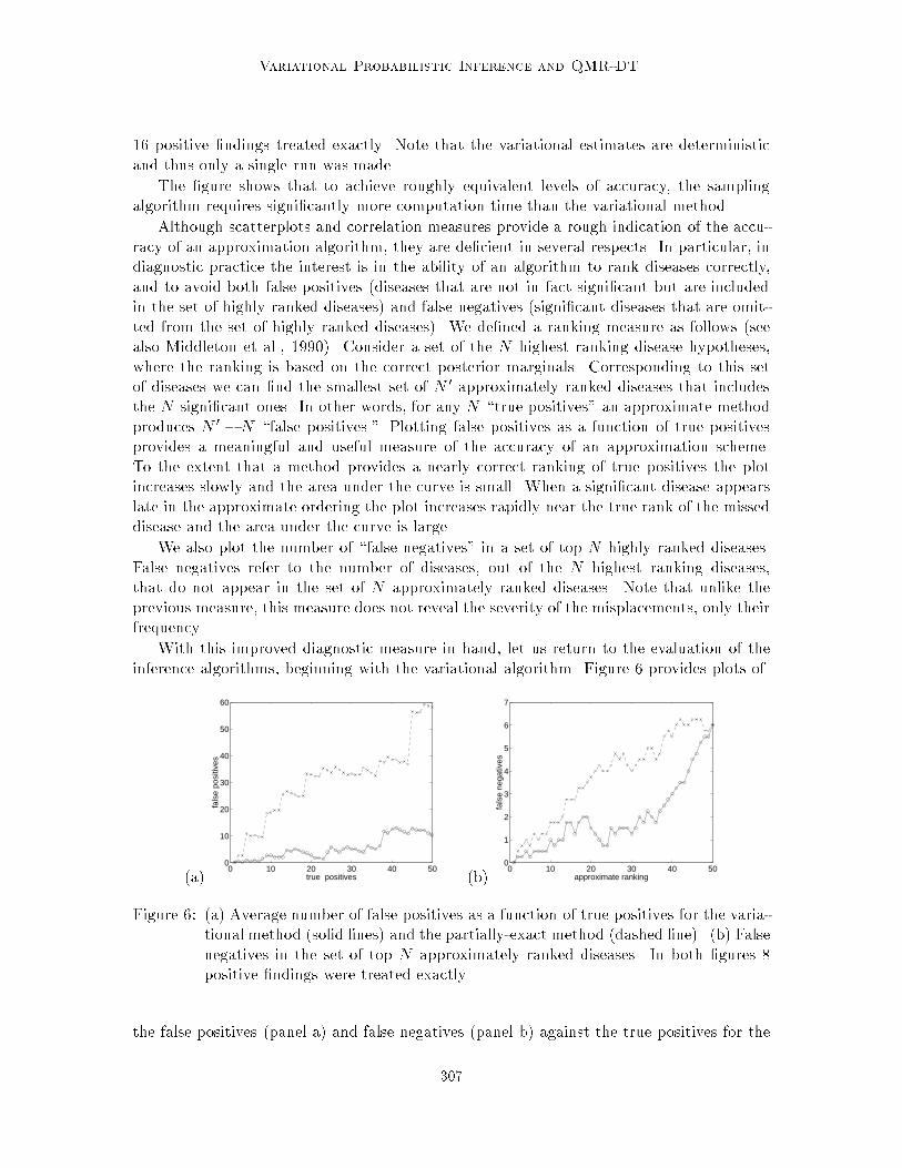
Although scatterplots and correlation measures provide a rough indication of the accu-racy of an approximation algorithm, they are de�cient in several respects. In particular, indiagnostic practice the interest is in the ability of an algorithm to rank diseases correctly,and to avoid both false positives (diseases that are not in fact signi�cant but are includedin the set of highly ranked diseases) and false negatives (signi�cant diseases that are omit-ted from the set of highly ranked diseases). We de�ned a ranking measure as follows (seealso Middleton et al., 1990). Consider a set of the N highest ranking disease hypotheses,where the ranking is based on the correct posterior marginals. Corresponding to this setof diseases we can �nd the smallest set of N 0 approximately ranked diseases that includesthe N signi�cant ones. In other words, for any N \true positives" an approximate methodproduces N 0 � N \false positives." Plotting false positives as a function of true positivesprovides a meaningful and useful measure of the accuracy of an approximation scheme.To the extent that a method provides a nearly correct ranking of true positives the plotincreases slowly and the area under the curve is small. When a signi�cant disease appearslate in the approximate ordering the plot increases rapidly near the true rank of the misseddisease and the area under the curve is large.

We also plot the number of \false negatives" in a set of top N highly ranked diseases.False negatives refer to the number of diseases, out of the N highest ranking diseases,that do not appear in the set of N approximately ranked diseases. Note that unlike theprevious measure, this measure does not reveal the severity of the misplacements, only theirfrequency.

With this improved diagnostic measure in hand, let us return to the evaluation of theinference algorithms, beginning with the variational algorithm. Figure 6 provides plots of

(a)0 10 20 30 40 50

0

10

20

30

40

50

60

true positives

fals

e po

sitiv

es

(b)0 10 20 30 40 50

0

1

2

3

4

5

6

7

approximate ranking

fals

e ne

gativ

es

Figure 6: (a) Average number of false positives as a function of true positives for the varia-tional method (solid lines) and the partially-exact method (dashed line). (b) Falsenegatives in the set of top N approximately ranked diseases. In both �gures 8positive �ndings were treated exactly.

the false positives (panel a) and false negatives (panel b) against the true positives for the

307

Jaakkola & Jordan

(a)0 10 20 30 40 50

0

5

10

15

20

25

30

35

40

true positives

fals

e po

sitiv

es

(b)0 10 20 30 40 50

0

0.5

1

1.5

2

2.5

3

3.5

4

approximate ranking

fals

e ne

gativ

es

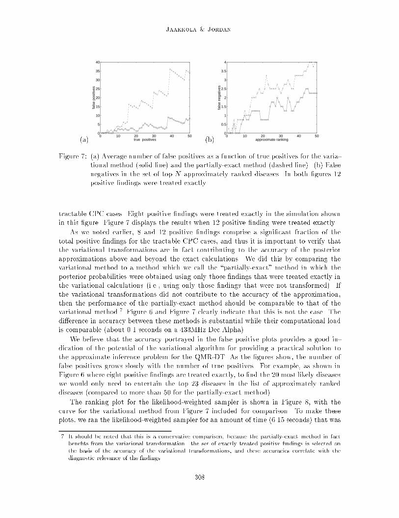
Figure 7: (a) Average number of false positives as a function of true positives for the varia-tional method (solid line) and the partially-exact method (dashed line). (b) Falsenegatives in the set of top N approximately ranked diseases. In both �gures 12positive �ndings were treated exactly.

tractable CPC cases. Eight positive �ndings were treated exactly in the simulation shownin this �gure. Figure 7 displays the results when 12 positive �nding were treated exactly.

As we noted earlier, 8 and 12 positive �ndings comprise a signi�cant fraction of thetotal positive �ndings for the tractable CPC cases, and thus it is important to verify thatthe variational transformations are in fact contributing to the accuracy of the posteriorapproximations above and beyond the exact calculations. We did this by comparing thevariational method to a method which we call the \partially-exact" method in which theposterior probabilities were obtained using only those �ndings that were treated exactly inthe variational calculations (i.e., using only those �ndings that were not transformed). Ifthe variational transformations did not contribute to the accuracy of the approximation,then the performance of the partially-exact method should be comparable to that of thevariational method.7 Figure 6 and Figure 7 clearly indicate that this is not the case. Thedi�erence in accuracy between these methods is substantial while their computational loadis comparable (about 0.1 seconds on a 433MHz Dec Alpha).

We believe that the accuracy portrayed in the false positive plots provides a good in-dication of the potential of the variational algorithm for providing a practical solution tothe approximate inference problem for the QMR-DT. As the �gures show, the number offalse positives grows slowly with the number of true positives. For example, as shown inFigure 6 where eight positive �ndings are treated exactly, to �nd the 20 most likely diseaseswe would only need to entertain the top 23 diseases in the list of approximately rankeddiseases (compared to more than 50 for the partially-exact method).

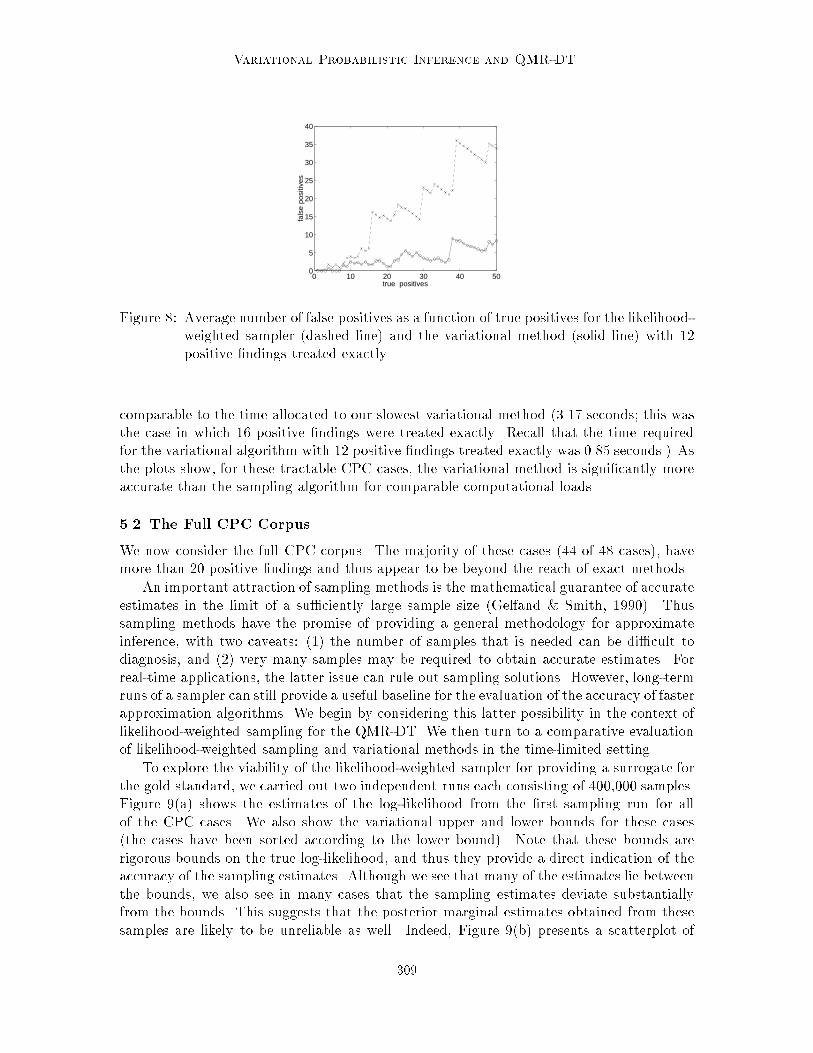
The ranking plot for the likelihood-weighted sampler is shown in Figure 8, with thecurve for the variational method from Figure 7 included for comparison. To make theseplots, we ran the likelihood-weighted sampler for an amount of time (6.15 seconds) that was

7. It should be noted that this is a conservative comparison, because the partially-exact method in factbene�ts from the variational transformation|the set of exactly treated positive �ndings is selected onthe basis of the accuracy of the variational transformations, and these accuracies correlate with thediagnostic relevance of the �ndings.

308


0 10 20 30 40 500

5

10

15

20

25

30

35

40

true positives

fals

e po

sitiv

es

Figure 8: Average number of false positives as a function of true positives for the likelihood-weighted sampler (dashed line) and the variational method (solid line) with 12positive �ndings treated exactly.

comparable to the time allocated to our slowest variational method (3.17 seconds; this wasthe case in which 16 positive �ndings were treated exactly. Recall that the time requiredfor the variational algorithm with 12 positive �ndings treated exactly was 0.85 seconds.) Asthe plots show, for these tractable CPC cases, the variational method is signi�cantly moreaccurate than the sampling algorithm for comparable computational loads.

5.2 The Full CPC Corpus

We now consider the full CPC corpus. The majority of these cases (44 of 48 cases), havemore than 20 positive �ndings and thus appear to be beyond the reach of exact methods.

An important attraction of sampling methods is the mathematical guarantee of accurateestimates in the limit of a su�ciently large sample size (Gelfand & Smith, 1990). Thussampling methods have the promise of providing a general methodology for approximateinference, with two caveats: (1) the number of samples that is needed can be di�cult todiagnosis, and (2) very many samples may be required to obtain accurate estimates. Forreal-time applications, the latter issue can rule out sampling solutions. However, long-termruns of a sampler can still provide a useful baseline for the evaluation of the accuracy of fasterapproximation algorithms. We begin by considering this latter possibility in the context oflikelihood-weighted sampling for the QMR-DT. We then turn to a comparative evaluationof likelihood-weighted sampling and variational methods in the time-limited setting.

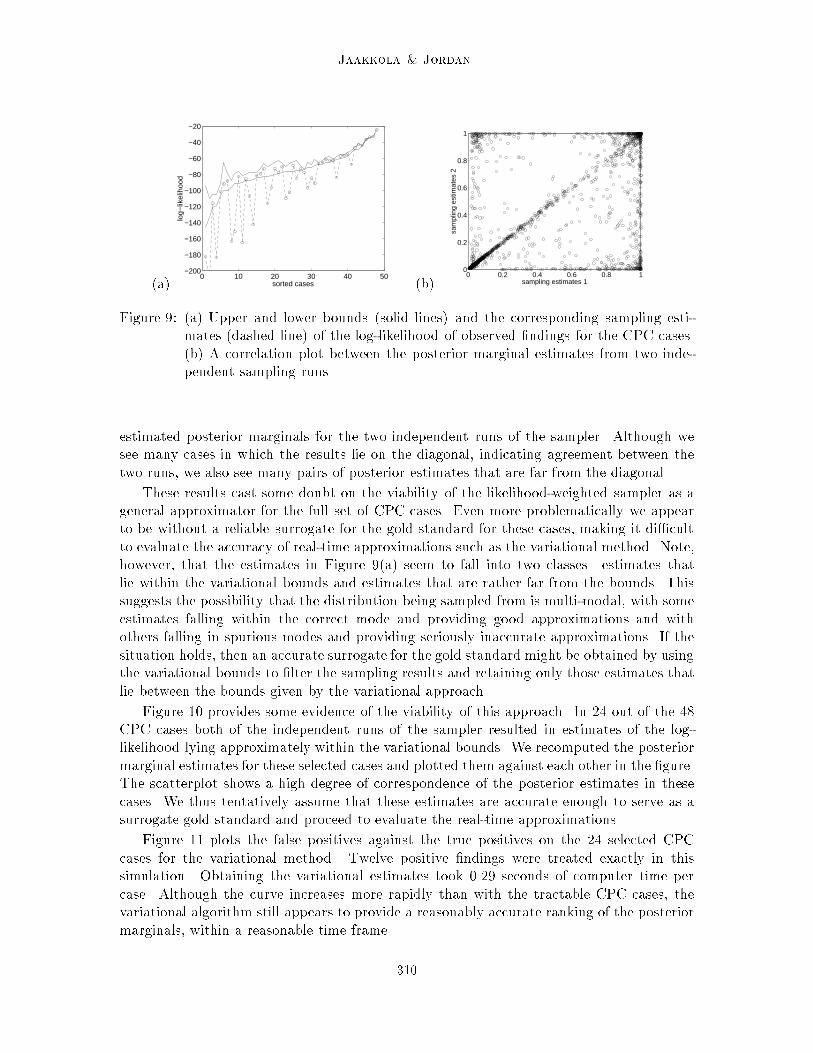
To explore the viability of the likelihood-weighted sampler for providing a surrogate forthe gold standard, we carried out two independent runs each consisting of 400,000 samples.Figure 9(a) shows the estimates of the log-likelihood from the �rst sampling run for allof the CPC cases. We also show the variational upper and lower bounds for these cases(the cases have been sorted according to the lower bound). Note that these bounds arerigorous bounds on the true log-likelihood, and thus they provide a direct indication of theaccuracy of the sampling estimates. Although we see that many of the estimates lie betweenthe bounds, we also see in many cases that the sampling estimates deviate substantiallyfrom the bounds. This suggests that the posterior marginal estimates obtained from thesesamples are likely to be unreliable as well. Indeed, Figure 9(b) presents a scatterplot of

309

Jaakkola & Jordan

(a)0 10 20 30 40 50

−200

−180

−160

−140

−120

−100

−80

−60

−40

−20

sorted cases

log−

likel

ihoo

d

(b)0 0.2 0.4 0.6 0.8 1

0

0.2

0.4

0.6

0.8

1

sampling estimates 1

sam

plin

g es

timat

es 2

Figure 9: (a) Upper and lower bounds (solid lines) and the corresponding sampling esti-mates (dashed line) of the log-likelihood of observed �ndings for the CPC cases.(b) A correlation plot between the posterior marginal estimates from two inde-pendent sampling runs.

estimated posterior marginals for the two independent runs of the sampler. Although wesee many cases in which the results lie on the diagonal, indicating agreement between thetwo runs, we also see many pairs of posterior estimates that are far from the diagonal.

These results cast some doubt on the viability of the likelihood-weighted sampler as ageneral approximator for the full set of CPC cases. Even more problematically we appearto be without a reliable surrogate for the gold standard for these cases, making it di�cultto evaluate the accuracy of real-time approximations such as the variational method. Note,however, that the estimates in Figure 9(a) seem to fall into two classes|estimates thatlie within the variational bounds and estimates that are rather far from the bounds. Thissuggests the possibility that the distribution being sampled from is multi-modal, with someestimates falling within the correct mode and providing good approximations and withothers falling in spurious modes and providing seriously inaccurate approximations. If thesituation holds, then an accurate surrogate for the gold standard might be obtained by usingthe variational bounds to �lter the sampling results and retaining only those estimates thatlie between the bounds given by the variational approach.

Figure 10 provides some evidence of the viability of this approach. In 24 out of the 48CPC cases both of the independent runs of the sampler resulted in estimates of the log-likelihood lying approximately within the variational bounds. We recomputed the posteriormarginal estimates for these selected cases and plotted them against each other in the �gure.The scatterplot shows a high degree of correspondence of the posterior estimates in thesecases. We thus tentatively assume that these estimates are accurate enough to serve as asurrogate gold standard and proceed to evaluate the real-time approximations.

Figure 11 plots the false positives against the true positives on the 24 selected CPCcases for the variational method. Twelve positive �ndings were treated exactly in thissimulation. Obtaining the variational estimates took 0.29 seconds of computer time percase. Although the curve increases more rapidly than with the tractable CPC cases, thevariational algorithm still appears to provide a reasonably accurate ranking of the posteriormarginals, within a reasonable time frame.

310


0 0.2 0.4 0.6 0.8 10

0.2

0.4

0.6

0.8

1

sampling estimates 1

sam

plin

g es

timat

es 2

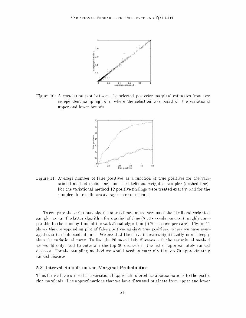
Figure 10: A correlation plot between the selected posterior marginal estimates from twoindependent sampling runs, where the selection was based on the variationalupper and lower bounds.

0 10 20 30 40 500

10

20

30

40

50

60

70

true positives

fals

e po

sitiv

es

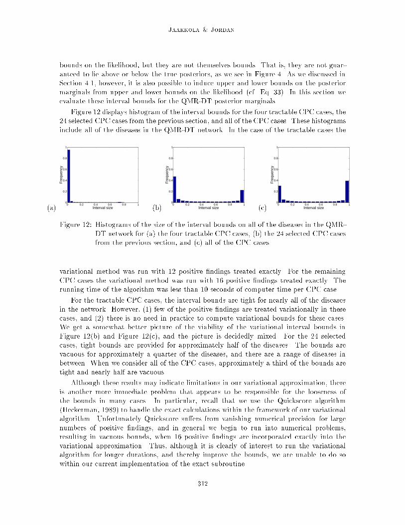
Figure 11: Average number of false positives as a function of true positives for the vari-ational method (solid line) and the likelihood-weighted sampler (dashed line).For the variational method 12 positive �ndings were treated exactly, and for thesampler the results are averages across ten runs.

To compare the variational algorithm to a time-limited version of the likelihood-weightedsampler we ran the latter algorithm for a period of time (8.83 seconds per case) roughly com-parable to the running time of the variational algorithm (0.29 seconds per case). Figure 11shows the corresponding plot of false positives against true positives, where we have aver-aged over ten independent runs. We see that the curve increases signi�cantly more steeplythan the variational curve. To �nd the 20 most likely diseases with the variational methodwe would only need to entertain the top 30 diseases in the list of approximately rankeddiseases. For the sampling method we would need to entertain the top 70 approximatelyranked diseases.

5.3 Interval Bounds on the Marginal Probabilities

Thus far we have utilized the variational approach to produce approximations to the poste-rior marginals. The approximations that we have discussed originate from upper and lower

311

Jaakkola & Jordan

bounds on the likelihood, but they are not themselves bounds. That is, they are not guar-anteed to lie above or below the true posteriors, as we see in Figure 4. As we discussed inSection 4.1, however, it is also possible to induce upper and lower bounds on the posteriormarginals from upper and lower bounds on the likelihood (cf. Eq. 33). In this section weevaluate these interval bounds for the QMR-DT posterior marginals.

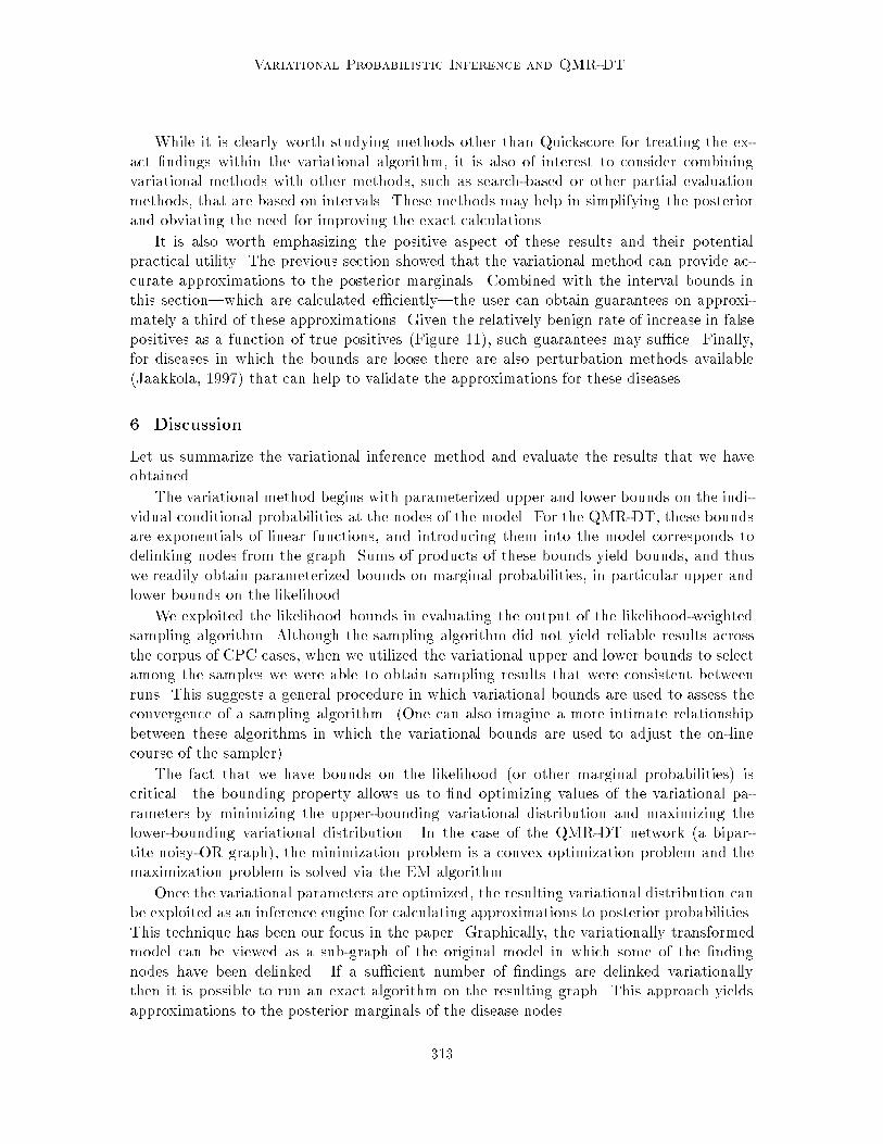
Figure 12 displays histogram of the interval bounds for the four tractable CPC cases, the24 selected CPC cases from the previous section, and all of the CPC cases. These histogramsinclude all of the diseases in the QMR-DT network. In the case of the tractable cases the

(a)0 0.2 0.4 0.6 0.8 1

0

0.2

0.4

0.6

0.8

1

Interval size

Fre

quen

cy

(b)0 0.2 0.4 0.6 0.8 1

0

0.2

0.4

0.6

0.8

1

Interval size

Fre

quen

cy

(c)0 0.2 0.4 0.6 0.8 1

0

0.2

0.4

0.6

0.8

1

Interval size

Fre

quen

cy

Figure 12: Histograms of the size of the interval bounds on all of the diseases in the QMR-DT network for (a) the four tractable CPC cases, (b) the 24 selected CPC casesfrom the previous section, and (c) all of the CPC cases.

variational method was run with 12 positive �ndings treated exactly. For the remainingCPC cases the variational method was run with 16 positive �ndings treated exactly. Therunning time of the algorithm was less than 10 seconds of computer time per CPC case.

For the tractable CPC cases, the interval bounds are tight for nearly all of the diseasesin the network. However, (1) few of the positive �ndings are treated variationally in thesecases, and (2) there is no need in practice to compute variational bounds for these cases.We get a somewhat better picture of the viability of the variational interval bounds inFigure 12(b) and Figure 12(c), and the picture is decidedly mixed. For the 24 selectedcases, tight bounds are provided for approximately half of the diseases. The bounds arevacuous for approximately a quarter of the diseases, and there are a range of diseases inbetween. When we consider all of the CPC cases, approximately a third of the bounds aretight and nearly half are vacuous.

Although these results may indicate limitations in our variational approximation, thereis another more immediate problem that appears to be responsible for the looseness ofthe bounds in many cases. In particular, recall that we use the Quickscore algorithm(Heckerman, 1989) to handle the exact calculations within the framework of our variationalalgorithm. Unfortunately Quickscore su�ers from vanishing numerical precision for largenumbers of positive �ndings, and in general we begin to run into numerical problems,resulting in vacuous bounds, when 16 positive �ndings are incorporated exactly into thevariational approximation. Thus, although it is clearly of interest to run the variationalalgorithm for longer durations, and thereby improve the bounds, we are unable to do sowithin our current implementation of the exact subroutine.

312


While it is clearly worth studying methods other than Quickscore for treating the ex-act �ndings within the variational algorithm, it is also of interest to consider combiningvariational methods with other methods, such as search-based or other partial evaluationmethods, that are based on intervals. These methods may help in simplifying the posteriorand obviating the need for improving the exact calculations.

It is also worth emphasizing the positive aspect of these results and their potentialpractical utility. The previous section showed that the variational method can provide ac-curate approximations to the posterior marginals. Combined with the interval bounds inthis section|which are calculated e�ciently|the user can obtain guarantees on approxi-mately a third of these approximations. Given the relatively benign rate of increase in falsepositives as a function of true positives (Figure 11), such guarantees may su�ce. Finally,for diseases in which the bounds are loose there are also perturbation methods available(Jaakkola, 1997) that can help to validate the approximations for these diseases.

6. Discussion

Let us summarize the variational inference method and evaluate the results that we haveobtained.

The variational method begins with parameterized upper and lower bounds on the indi-vidual conditional probabilities at the nodes of the model. For the QMR-DT, these boundsare exponentials of linear functions, and introducing them into the model corresponds todelinking nodes from the graph. Sums of products of these bounds yield bounds, and thuswe readily obtain parameterized bounds on marginal probabilities, in particular upper andlower bounds on the likelihood.

We exploited the likelihood bounds in evaluating the output of the likelihood-weightedsampling algorithm. Although the sampling algorithm did not yield reliable results acrossthe corpus of CPC cases, when we utilized the variational upper and lower bounds to selectamong the samples we were able to obtain sampling results that were consistent betweenruns. This suggests a general procedure in which variational bounds are used to assess theconvergence of a sampling algorithm. (One can also imagine a more intimate relationshipbetween these algorithms in which the variational bounds are used to adjust the on-linecourse of the sampler).

The fact that we have bounds on the likelihood (or other marginal probabilities) iscritical|the bounding property allows us to �nd optimizing values of the variational pa-rameters by minimizing the upper-bounding variational distribution and maximizing thelower-bounding variational distribution. In the case of the QMR-DT network (a bipar-tite noisy-OR graph), the minimization problem is a convex optimization problem and themaximization problem is solved via the EM algorithm.

Once the variational parameters are optimized, the resulting variational distribution canbe exploited as an inference engine for calculating approximations to posterior probabilities.This technique has been our focus in the paper. Graphically, the variationally transformedmodel can be viewed as a sub-graph of the original model in which some of the �ndingnodes have been delinked. If a su�cient number of �ndings are delinked variationallythen it is possible to run an exact algorithm on the resulting graph. This approach yieldsapproximations to the posterior marginals of the disease nodes.

313

Jaakkola & Jordan

We found empirically that these approximations appeared to provide good approxima-tions to the true posterior marginals. This was the case for the tractable set of CPC cases(cf. Figure 7) and|subject to our assumption that we have obtained a good surrogate forthe gold standard via the selected output of the sampler|also the case for the full CPCcorpus (cf. Figure 11).

We also compared the variational algorithm to a state-of-the-art algorithm for the QMR-DT, the likelihood-weighted sampler of Shwe and Cooper (1991). We found that the varia-tional algorithm outperformed the likelihood-weighted sampler both for the tractable casesand for the full corpus. In particular, for a �xed accuracy requirement the variational algo-rithm was signi�cantly faster (cf. Figure 5), and for a �xed time allotment the variationalalgorithm was signi�cantly more accurate (cf. Figure 8 and Figure 11).

Our results were less satisfactory for the interval bounds on the posterior marginals.Across the full CPC corpus we found that for approximately one third of the disease thebounds were tight but for half of the diseases the bounds were vacuous. A major impedimentto obtaining tighter bounds appears to lie not in the variational approximation per se butrather in the exact subroutine, and we are investigating exact methods with improvednumerical properties.

Although we have focused in detail on the QMR-DT model in this paper, it is worthnoting that the variational probabilistic inference methodology is considerably more general.Speci�cally, the methods that we have described here are not limited to the bi-partitegraphical structure of the QMR-DT model, nor is it necessary to employ noisy-OR nodes(Jaakkola & Jordan, 1996). It is also the case that the type of transformations that wehave exploited in the QMR-DT setting extend to a larger class of dependence relationsbased on generalized linear models (Jaakkola, 1997). Finally, for a review of applications ofvariational methods to a variety of other graphical model architectures, see Jordan, et al.(1998).

A promising direction for future research appears to be in the integration of variouskinds of approximate and exact methods (see, e.g., Dagum & Horvitz, 1992; Jensen, Kong,& Kj�rul�, 1995). In particular, search-based methods (Cooper, 1985; Peng & Reggia,1987, Henrion, 1991) and variational methods both yield bounds on probabilities, and, aswe have indicated in the introduction, they seem to exploit di�erent aspects of the struc-ture of complex probability distributions. It may be possible to combine the bounds fromthese algorithm|the variational bounds might be used to guide the search, or the search-based bounds might be used to aid the variational approximation. Similar comments canbe made with respect to localized partial evaluation methods and bounded conditioningmethods (Draper & Hanks, 1994; Horvitz, et al., 1989). Also, we have seen that variationalbounds can be used for assessing whether estimates from Monte Carlo sampling algorithmshave converged. A further interesting hybrid would be a scheme in which variational ap-proximations are re�ned by treating them as initial conditions for a sampler.

Even without extensions our results in this paper appear quite promising. We havepresented an algorithm which runs in real time on a large-scale graphical model for whichexact algorithms are in general infeasible. The results that we have obtained appear tobe reasonably accurate across a corpus of di�cult diagnostic cases. While further workis needed, we believe that our results indicate a promising role for variational inference indeveloping, critiquing and exploiting large-scale probabilistic models such as the QMR-DT.

314


Acknowledgements

We would like to thank the University of Pittsburgh and Randy Miller for the use of theQMR-DT database. We also want to thank David Heckerman for suggesting that we attackQMR-DT with variational methods, and for providing helpful counsel along the way.

Appendix A. Duality

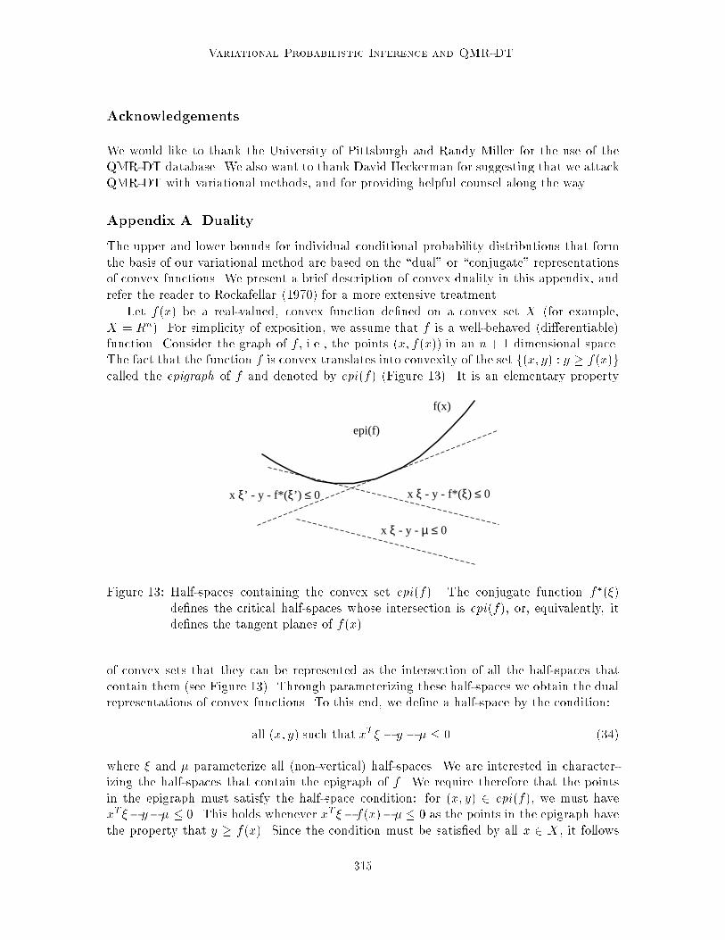
The upper and lower bounds for individual conditional probability distributions that formthe basis of our variational method are based on the \dual" or \conjugate" representationsof convex functions. We present a brief description of convex duality in this appendix, andrefer the reader to Rockafellar (1970) for a more extensive treatment.

Let f(x) be a real-valued, convex function de�ned on a convex set X (for example,X = Rn). For simplicity of exposition, we assume that f is a well-behaved (di�erentiable)function. Consider the graph of f , i.e., the points (x; f(x)) in an n + 1 dimensional space.The fact that the function f is convex translates into convexity of the set f(x; y) : y � f(x)gcalled the epigraph of f and denoted by epi(f) (Figure 13). It is an elementary property

f(x)

epi(f)

x ξ - y - f*(ξ) ≤ 0x ξ’ - y - f*( ξ’) ≤ 0

x ξ - y - µ ≤ 0

Figure 13: Half-spaces containing the convex set epi(f). The conjugate function f�(�)de�nes the critical half-spaces whose intersection is epi(f), or, equivalently, itde�nes the tangent planes of f(x).

of convex sets that they can be represented as the intersection of all the half-spaces thatcontain them (see Figure 13). Through parameterizing these half-spaces we obtain the dualrepresentations of convex functions. To this end, we de�ne a half-space by the condition:

all (x; y) such that xT � � y � � � 0 (34)

where � and � parameterize all (non-vertical) half-spaces. We are interested in character-izing the half-spaces that contain the epigraph of f . We require therefore that the pointsin the epigraph must satisfy the half-space condition: for (x; y) 2 epi(f), we must havexT��y�� 0. This holds whenever xT ��f(x)�� 0 as the points in the epigraph havethe property that y � f(x). Since the condition must be satis�ed by all x 2 X , it follows

315

Jaakkola & Jordan

that

maxx2Xf xT� � f(x)� � g � 0; (35)

as well. Equivalently,

� � maxx2Xf xT � � f(x) g (36)

where the right-hand side of this equation de�nes a function of �, which is known as the\dual" or \conjugate" function f�(�). This function, which is also a convex function, de�nesthe critical half-spaces which are needed for the representation of epi(f) as an intersectionof half-spaces (Figure 13).

To clarify the duality between f(x) and f�(x), let us drop the maximum and rewritethe inequality as:

xT � � f(x) + f�(�) (37)

In this equation, the roles of the two functions are interchangeable and we may suspect thatalso f(x) can obtained from the dual function f�(x) by an optimization procedure. This isin fact the case and we have:

f(x) = max�2�f xT� � f�(�) g (38)

This equality states that the dual of the dual gives back the original function. It providesthe computational tool for calculating dual functions.

For concave (convex down) functions the results are analogous; we replace max withmin, and lower bounds with upper bounds.

Appendix B. Optimization of the Variational Parameters

The variational method that we have described involves replacing selected local conditionalprobabilities with either upper-bounding or lower-bounding variational transformations.Because the product of bounds is a bound, the variationally transformed joint probabilitydistribution is a bound (upper or lower) on the true joint probability distribution. More-over, because sums of bounds is a bound on the sum, we can obtain bounds on marginalprobabilities by marginalizing the variationally transformed joint probability distribution.In particular, this provides a method for obtaining bounds on the likelihood (the marginalprobability of the evidence).

Note that the variationally transformed distributions are bounds for arbitrary values ofthe variational parameters (because each individually transformed node conditional prob-ability is a bound for arbitrary values of its variational parameter). To obtain optimizingvalues of the variational parameters, we take advantage of the fact that our transformeddistribution is a bound, and either minimize (in the case of upper bounds) or maximize(in the case of lower bounds) the transformed distribution with respect to the variationalparameters. It is this optimization process which provides a tight bound on the marginalprobability of interest (e.g., the likelihood) and thereby picks out a particular variationaldistribution that can subsequently be used for approximate inference.

316


In this appendix we discuss the optimization problems that we must solve in the caseof noisy-OR networks. We consider the upper and lower bounds separately, beginning withthe upper bound.

Upper Bound Transformations

Our goal is to compute a tight upper bound on the likelihood of the observed �ndings:P (f+) =

Pd P (f

+jd)P (d). As discussed in Section 4.2, we obtain an upper bound onP (f+jd) by introducing upper bounds for individual node conditional probabilities. Werepresent this upper bound as P (f+jd; �), which is a product across the individual varia-tional transformations and may contain contributions due to �ndings that are being treatedexactly (i.e., are not transformed). Marginalizing across d we obtain a bound:

P (f+) �Xd

P (f+jd; �)P (d) � P (f+j�): (39)

It is this latter quantity that we wish to minimize with respect to the variational parameters�.

To simplify the notation we assume that the �rst m positive �ndings have been trans-formed (and therefore need to be optimized) while the remaining conditional probabilitieswill be treated exactly. In this notation P (f+j�) is given by

P (f+j�) =Xd

24Yi�m

P (f+i jd; �i)

35"Y

i>m

P (f+i jd)

#Yj

P (dj) (40)

/ E

8<:Yi�m

P (f+i jd; �i)

9=; ; (41)

where the expectation is taken with respect to the posterior distribution for the diseasesgiven those positive �ndings that we plan to treat exactly. Note that the proportionalityconstant does not depend on the variational parameters (it is the likelihood of the exactlytreated positive �ndings). We now insert the explicit forms of the transformed conditionalprobabilities (see Eq. (17)) into Eq. (41) and �nd:

P (f+j�) / E

8<:Yi�m

e�i(�i0+

Pj�ijdj)�f�(�i)

9=; (42)

= eP

i�m(�i�i0�f�(�i))E

�eP

j; i�m�i�ijdj

�(43)

where we have simply converted the products over i into sums in the exponent and pulledout the terms that are constants with respect to the expectation. On a log-scale, theproportionality becomes an equivalence up to a constant:

logP (f+j�) = C +Xi�m

(�i�i0 � f�(�i)) + logE

�eP

j;i�m�i�ijdj

�(44)

317

Jaakkola & Jordan

Several observations are in order. Recall that f�(�i) is the conjugate of the concave functionf (the exponent), and is therefore also concave; for this reason �f�(�i) is convex. InAppendix C we prove that the remaining term:

logE

�eP

j;i�m�i�ijdj

�(45)

is also a convex function of the variational parameters. Now, since any sum of convexfunctions is convex, we conclude that logP (f+j�) is a convex function of the variationalparameters. This means that there are no local minima in our optimization problem. Wemay safely employ the standard Newton-Raphson procedure to solve r logP (f+j�) = 0.Alternatively we can utilize �xed-point iterations. In particular, we calculate the derivativesof the variational form and iteratively solve for the individual variational parameters �k suchthat the derivatives are zero. The derivatives are given as follows:

@

@�klogP (f+j�) = �k0 + log

�k1 + �k

+ E

8<:Xj

�kjdj

9=; (46)

@2

@2�klogP (f+j�) =

1

�k�

1

1 + �k+Var

8<:Xj

�kjdj

9=; ; (47)

where the expectation and the variance are with respect to the posterior approximationP (djf+; �), and both derivatives can be computed in time linear in the number of associ-ated diseases for the �nding. The benign scaling of the variance calculations comes fromexploiting the special properties of the noisy-OR dependence and the marginal independenceof the diseases.

Calculating the expectations in Eq. (7) is exponentially costly in the number of exactlytreated positive �ndings. When there are a large number of positive �ndings, we can haverecourse to a simpli�ed procedure in which we optimize variational parameters after havingtransformed all or most of the positive �ndings. While the resulting variational parametersare suboptimal, we have found in practice that the incurred loss in accuracy is typically quitesmall. In the simulations reported in the paper, we optimized the variational parametersafter approximately half of the exactly treated �ndings had been introduced. (To be precise,in the case of 8, 12 and 16 total �ndings treated exactly, we optimized the parameters after4, 8, and 8 �ndings, respectively, were introduced).

Lower Bound Transformations

Mimicking the case of upper bounds, we replace individual conditional probabilities ofthe �ndings with lower-bounding transformations, resulting in a lower-bounding expressionP (f+jd; q). Taking the product with P (d) and marginalizing over d yields a lower boundon the likelihood:

P (f+) �Xd

P (f+jd; q)P (d) � P (f+jq): (48)

We wish to maximize P (f+jq) with respect to the variational parameters q to obtain thetightest possible bound.

318


Our problem can be mapped onto a standard optimization problem in statistics. Inparticular, treating d as a latent variable, f as an observed variable, and q as a parametervector, the optimization of P (f+jq) (or its logarithm) can be viewed as a standard maximumlikelihood estimation problem for a latent variable model. It can be solved using the EMalgorithm (Dempster, Laird, & Rubin, 1977). The algorithm yields a sequence of variationalparameters that monotonically increase the objective function logP (f+jq). Within the EMframework, we obtain an update of the variational parameters by maximizing the expectedcomplete log-likelihood:

E�log P (f+jd; q)P (d)

=Xi

EnlogP (f+i jd; q�ji)

o+ constant; (49)

where qold denotes the vector of variational parameters before the update, where the con-stant term is independent of the variational parameters q and where the expectation is withrespect to the posterior distribution P (djf+; qold) / P (f+jd; qold)P (d). Since the variationalparameters associated with the conditional probabilities P (f+i jd; q�ji) are independent of oneanother, we can maximize each term in the above sum separately. Recalling the form of thevariational transformation (see Eq. (24)), we have:

Enlog P (f+i jd; q�ji)

o=

Xj

qjjiEfdjg

"f

�io +

�ijqjji

!� f ( �io )

#

+f ( �io ) (50)

which we are to maximize with respect to qjji while keeping the expectations Efdjg �xed.This optimization problem can be solved iteratively and monotonically by performing thefollowing synchronous updates with normalization:

qjji Efdjg

"qjji f

�io +

�ijqjji

!� �ij f

0

�io +

�ijqjji

!� qjji f( �io )

#

(51)

where f 0 denotes the derivative of f . (The update is guaranteed to be non-negative).This algorithm can be easily extended to handle the case where not all the positive

�ndings have been transformed. The only new feature is that some of the conditionalprobabilities in the products P (f+jd; qold) and P (f+jd; q) have been left intact, i.e., nottransformed; the optimization with respect to the variational parameters corresponding tothe transformed conditionals proceeds as before.

Appendix C. Convexity

The purpose of this appendix is to demonstrate that the function:

logE

�eP

j;i�m�i�ijdj

�(52)

is a convex function of the variational parameters �i. We note �rst that a�ne transforma-tions do not change convexity properties. Thus convexity in X =

Pj;i�m �i�ijdj implies

319

Jaakkola & Jordan

convexity in the variational parameters �. It remains to show that

logEneXo= log

Xi

pi eXi = f( ~X) (53)

is a convex function of the vector ~X = fX1 : : :XngT ; here we have indicated the discrete

values in the range of the random variable X by Xi and denoted the probability measureon such values by pi. Taking the gradient of f with respect to Xk gives:

@

@Xk

f( ~X) =pke

XkPi pi e

Xi� qk (54)

where qk de�nes a probability distribution. The convexity is revealed by a positive semi-de�nite Hessian H, whose components in this case are

Hkl =@2

@Xk@Xl

f( ~X) = �klqk � qkql (55)

To see that H is positive semi-de�nite, consider

~ZTH ~Z =Xk

qkZ2k � (

Xk

qkZk)(Xl

qlZl) = VarfZg � 0 (56)

where VarfZg is the variance of a discrete random variable Z which takes the values Zi

with probability qi.

References

D'Ambrosio, B. (1993). Incremental probabilistic inference. In Proceedings of the Ninth

Conference on Uncertainty in Arti�cial Intelligence. San Mateo, CA: Morgan Kauf-mann.

D'Ambrosio, B. (1994). Symbolic probabilistic inference in large BN20 networks. In Pro-

ceedings of the Tenth Conference on Uncertainty in Arti�cial Intelligence. San Mateo,CA: Morgan Kaufmann.

Cooper, G. (1985). NESTOR: A computer-based medical diagnostic aid that integrates

causal and probabilistic knowledge. Ph.D. Dissertation, Medical Informatics Sciences,Stanford University, Stanford, CA. (Available from UMI athttp://wwwlib.umi.com/dissertations/main).

Cooper, G. (1990). The computational complexity of probabilistic inference using Bayesianbelief networks. Arti�cial Intelligence, 42, 393{405.

Dagum, P., & Horvitz, E. (1992). Reformulating inference problems through selectiveconditioning. In Proceedings of the Eighth Annual Conference on Uncertainty in

Arti�cial Intelligence.

Dagum, P., & Horvitz, E. (1993). A Bayesian analysis of simulation algorithms for inferencein Belief networks. Networks, 23, 499{516.

320


Dagum, P., & Luby, M. (1993). Approximate probabilistic reasoning in Bayesian beliefnetworks is NP-hard. Arti�cial Intelligence, 60, 141{153.

Dechter, R. (1997). Mini-buckets: A general scheme of generating approximations in auto-mated reasoning. In Proceedings of the Fifteenth International Joint Conference on

Arti�cial Intelligence.

Dechter, R. (1998). Bucket elimination: A unifying framework for probabilistic inference.In M. I. Jordan (Ed.), Learning in Graphical Models. Cambridge, MA: MIT Press.

Dempster, A., Laird, N., & Rubin, D. (1977). Maximum likelihood from incomplete datavia the EM algorithm. Journal of the Royal Statistical Society B, 39, 1{38.

Draper, D., & Hanks, S. (1994). Localized partial evaluation of belief networks. In Pro-

ceedings of the Tenth Annual Conference on Uncertainty in Arti�cial Intelligence.

Fung, R., & Chang, K. C. (1990). Weighting and integrating evidence for stochastic sim-ulation in Bayesian networks. In Proceedings of Fifth Conference on Uncertainty in

Arti�cial Intelligence. Amsterdam: Elsevier Science.

Gelfand, A., & Smith, A. (1990). Sampling-based approaches to calculating marginal Den-sities. Journal of the American Statistical Association, 85, 398{409.

Heckerman, D. (1989). A tractable inference algorithm for diagnosing multiple diseases. InProceedings of the Fifth Conference on Uncertainty in Arti�cial Intelligence.

Henrion, M. (1991). Search-based methods to bound diagnostic probabilities in very largebelief nets. In Proceedings of Seventh Conference on Uncertainty in Arti�cial Intelli-

gence.

Horvitz, E. Suermondt, H., & Cooper, G. (1989). Bounded conditioning: Flexible inferencefor decisions under scarce resources. In Proceedings of Fifth Conference on Uncer-

tainty in Arti�cial Intelligence.

Jaakkola, T. (1997). Variational methods for inference and learning in graphical models.PhD thesis, Department of Brain and Cognitive Sciences, Massachusetts Institute ofTechnology.

Jaakkola, T., & Jordan, M. (1996). Recursive algorithms for approximating probabilitiesin graphical models. In Advances of Neural Information Processing Systems 9. Cam-bridge, MA: MIT Press.

Jensen, C. S., Kong, A., & Kj�rul�, U. (1995). Blocking-Gibbs sampling in very largeprobabilistic expert systems. International Journal of Human-Computer Studies, 42,647{666.

Jensen, F. (1996). Introduction to Bayesian networks. New York: Springer.

321

Jaakkola & Jordan

Jordan, M., Ghaharamani, Z. Jaakkola, T., & Saul, L. (in press). An introduction tovariational methods for graphical models. Machine Learning.

Lauritzen, S., & Spiegelhalter, D. (1988). Local computations with probabilities on graph-ical structures and their application to expert systems (with discussion). Journal of

the Royal Statistical Society B, 50, 157{224.

MacKay, D. J. C. (1998). Introduction to Monte Carlo methods. In M. I. Jordan (Ed.),Learning in Graphical Models. Cambridge, MA: MIT Press.

Middleton, B., Shwe, M., Heckerman, D., Henrion, M., Horvitz, E., Lehmann, H., & Cooper,G. (1990). Probabilistic diagnosis using a reformulation of the INTERNIST-1/QMRknowledge base II. Evaluation of diagnostic performance. Section on Medical Infor-matics Technical report SMI-90-0329, Stanford University.

Miller, R. A., Fasarie, F. E., & Myers, J. D. (1986). Quick medical reference (QMR) fordiagnostic assistance. Medical Computing, 3, 34{48.

Pearl, J. (1988). Probabilistic Reasoning in Intelligent Systems. San Mateo, CA: MorganKaufmann.

Peng, Y., & Reggia, J. (1987). A probabilistic causal model for diagnostic problem solving {Part 2: Diagnostic strategy. IEEE Trans. on Systems, Man, and Cybernetics: Special

Issue for Diagnosis, 17, 395{406.

Poole, D. (1997). Probabilistic partial evaluation: Exploiting rule structure in probabilisticinference. In Proceedings of the Fifteenth International Joint Conference on Arti�cial

Intelligence.

Rockafellar, R. (1972). Convex Analysis. Princeton University Press.

Shachter, R. D., & Peot, M. (1990). Simulation approaches to general probabilistic inferenceon belief networks. In Proceedings of Fifth Conference on Uncertainty in Arti�cial

Intelligence. Elsevier Science: Amsterdam.

Shenoy, P. P. (1992). Valuation-based systems for Bayesian decision analysis. Operations

Research, 40, 463{484.

Shwe, M., & Cooper, G. (1991). An empirical analysis of likelihood { weighting simulationon a large, multiply connected medical belief network. Computers and Biomedical

Research, 24, 453-475.

Shwe, M., Middleton, B., Heckerman, D., Henrion, M., Horvitz, E., Lehmann, H., & G.Cooper (1991). Probabilistic diagnosis using a reformulation of the INTERNIST-1/QMR knowledge base I. The probabilistic model and inference algorithms. Methods

of Information in Medicine, 30, 241{255.

322

journal of arti cial in telligence researc h 10 (1999) 291...

Documents