journal of banking and - rutgers...
TRANSCRIPT

Journal of Banking and Finance 73 (2016) 99–112
Contents lists available at ScienceDirect
Journal of Banking and Finance
journal homepage: www.elsevier.com/locate/jbf
Sovereign debt ratings and stock liquidity around the World
�
Kuan-Hui Lee
a , ∗, Horacio Sapriza
b , Yangru Wu
c , d
a Seoul National University Business School, 703 LG Building, 1 Kwanak-Ro, Kwanak-Gu, Seoul, 151-916, S. Korea b Federal Reserve Board, Division of International Finance, Washington, D.C. 20551, USA c Rutgers Business School – Newark and New Brunswick, Rutgers University, 1 Washington Park, Newark, NJ 07102, USA d Chinese Academy of Finance and Development, Central University of Finance and Economics
a r t i c l e i n f o
Article history:
Received 15 December 2015
Accepted 25 September 2016
Available online 28 September 2016
JEL classification:
G14
G15
Keywords:
Sovereign bond
Credit rating
Liquidity
Emerging market
Developed market
International financial market
a b s t r a c t
This paper studies the impact of sovereign debt rating changes on liquidity for stocks from 40 countries
for the period 1990–2009. We find that sovereign rating changes significantly affect stock liquidity. The
impact is stronger for downgrades than for upgrades, and is nonlinear in event size. The loss of invest-
ment grade has a particularly strong negative impact on stock liquidity. We also find that some stock
characteristics and country legal and macroeconomic environment are important in explaining the differ-
ences in the impact of sovereign credit rating changes on stock liquidity across countries.
© 2016 Elsevier B.V. All rights reserved.
1
i
c
e
t
r
c
t
t
e
v
M
F
S
t
S
G
c
a
r
g
a
f
i
i
h
m
e
2
h
0
. Introduction
Sovereign credit ratings provide assessments of the probabil-
ty of default in government debt. When rating a sovereign bond,
redit rating agencies state that they consider a large number of
conomic and political factors and make qualitative and quantita-
ive evaluations of the security. Consequently, a sovereign credit
ating change may unveil important new information about a
ountry and impose a significant externality to its private sec-
or, which can affect investors’ incentives to hold stocks. As ar-
� The authors are from: The views expressed in this paper are those of the au-
hors, and do not necessarily reflect those of the Federal Reserve Board or the Fed-
ral Reserve System. We thank conference and seminar participants at Central Uni-
ersity of Finance and Economics, International Conference on Asia-Pacific Financial
arkets, KAIST, Korea University, Seoul National University, Shanghai University of
inance and Economics, SNU Institute for Research in Finance and Economics, SKK
chool of Business, and Sun Yat–Sen University for helpful comments. Lee thanks
he Institute of Management Research and the Institute of Finance and Banking at
eoul National University. Wu thanks a Rutgers Business School Faculty Research
rant and the Whitcomb Center for Research in Financial Services for partial finan-
ial support. Part of this work was completed while Lee visited Cornell University
nd Wu visited the Central University of Finance and Economics, Beijing, China. All
emaining errors are our own. ∗ Corresponding author.
E-mail addresses: [email protected] (K.-H. Lee), [email protected]
(H. Sapriza), [email protected] (Y. Wu).
1
s
d
t
i
a
c
fi
1
t
s
c
s
ttp://dx.doi.org/10.1016/j.jbankfin.2016.09.011
378-4266/© 2016 Elsevier B.V. All rights reserved.
ued by Borensztein et al. (2007) and Gande and Parsley (2005) ,
mong others, the cost of sovereign debt constitutes a benchmark
or domestic interest rates, e.g., for the cost of corporate borrow-
ng. Hence, developments in sovereign credit markets have broad
mplications for the overall economy.
The literature on sovereign rating changes and financial markets
as mostly focused on the effects of such externality on equity
arket index returns ( Kaminsky and Schmukler, 2002; Brooks
t al., 20 04; Martell, 20 05 ), individual stock returns ( Martell,
005; Correa et al., 2013 ), or bond yields ( Cantor and Packer,
996; Larraín et al., 1997; Gande and Parsley, 2005 ). Prior studies
uggest that sovereign downgrades are generally associated with
eclines and higher volatility of stock market returns. Surprisingly,
he impact of sovereign debt rating changes on stock liquidity
n global financial markets has not been explored. 1 This paper
ttempts to fill this gap in the literature. We study the impact of
hanges in sovereign credit ratings on daily stock liquidity at the
rm level for 40 developed and emerging markets from January
990 to December 2009. To the best of our knowledge, this is
he first study to empirically investigate the impact of sovereign
1 Odders-White and Ready (2006) study the contemporaneous relation between
tock liquidity and credit ratings as well as the predictive power of liquidity on
redit ratings in the U.S. market. On the contrary, we investigate the impact of
overeign debt rating changes on stock liquidity.

100 K.-H. Lee et al. / Journal of Banking and Finance 73 (2016) 99–112
p
f
t
l
e
i
l
a
v
p
p
t
d
g
t
s
a
d
s
o
p
c
s
h
o
d
S
3
c
2
s
e
s
c
t
t
a
p
c
(
s
m
m
a
l
e
t
i
a
e
t
t
f
a
t
a
r
s
debt rating changes on stock liquidity. We also identify key firm-
specific and country-level determinants of corporate stock liquidity
changes during sovereign credit events.
We posit that sovereign rating changes can affect stock liquidity
through at least three channels.
First, the funding constraints of traders or financial intermedi-
aries (e.g., hedge funds, banks, or market-makers) may affect or be
affected by market liquidity ( Brunnermeier and Pedersen, 2009 ).
Financial intermediaries make the market by absorbing liquidity
shocks subject to funding constraints via posted margins on collat-
eral. When a sovereign credit rating is downgraded and the mar-
ket declines, financial intermediaries will endure losses in collat-
eral values and, if funding constraints bind, margin limits will be
hit, thereby forcing agents to liquidate their positions. Moreover,
as long as institutional holders are subject to ownership restric-
tions based on credit ratings (by corporate governance or legal
mandate), a sovereign downgrade will either force the institutional
holder to liquidate its position, or will at least provide the institu-
tional holder with a strong incentive to do so. One trader hitting
his/her limit in one security can lead to falling prices and liquidity
in other securities, making other traders hit their respective lim-
its as well. Thus, the so-called “liquidity spirals” or “liquidity black
holes” can arise ( Morris and Shin, 2004; Brunnermeier and Peder-
sen, 2009 ).
A second linkage between sovereign debt rating changes and
stock liquidity can occur when investors try to rebalance their
portfolios across borders in the event of a rating change, which
induces cross-border capital flows ( Kim and Wu, 2008; Gande and
Parsley, 2010 ). Since sovereign downgrades lead to limited access
to international capital markets in the future ( Dittmar and Yuan,
2008 ), and more so in the presence of a sovereign rating ceiling,
which provides an upper limit for ratings of corporate bonds in
the country ( Cavallo and Valenzuela, 2010 ), investors may with-
draw their capital from the countries when the downgrade an-
nouncement is made. On the other hand, sovereign upgrades may
induce more capital flows into the country. Hence, the portfolio
rebalancing effect can associate both downgrades and upgrades in
sovereign debt ratings with drops in stock liquidity.
A third link between rating changes and stock liquidity can be
present through an information channel, similarly to Odders-White
and Ready (2006) , who find that low credit ratings are related to
large adverse selection, and hence to low liquidity in U.S. stocks.
Since credit rating agencies update the sovereign credit ratings
based on their evaluations of various economic and political factors
of the security and the country, a sovereign credit rating change
can deliver important new information about a country, lowering
information asymmetry and thus, enhancing liquidity. While both
upgrade and downgrade announcements are informational events,
however, there could be an asymmetric impact of rating changes
on the stock market between upgrades and downgrades. That is,
rating agencies are in general reluctant to give downgrades ( Becker
and Milbourn, 2011 ), hence, downgrades may contain more infor-
mation than upgrades, implying that downgrades may have a big-
ger impact on liquidity than upgrades. Furthermore, the larger the
magnitude of credit rating changes, the bigger the impact on stock
liquidity. However, an upgrade is often considered as containing
less of new information than a downgrade, or even no news. As a
result, the impact of an upgrade on liquidity will be limited. There-
fore, the asymmetric information channel in general posits that
sovereign debt rating changes may improve liquidity, and the ef-
fect of a sovereign debt downgrade should be larger than that of
an upgrade.
We investigate the cross-firm and cross-country variations in
the impact of sovereign rating changes, including changes in credit
outlook, on stock liquidity. We employ a regression framework
instead of the popular event-study framework in order to avoid
otential misleading interpretations of the results that may arise
rom event clustering ( Gande and Parsley, 2005 ). Our results show
hat sovereign rating changes have a significant impact on stock
iquidity, and that larger events have greater effects than smaller
vents. Moreover, we find that the effect is asymmetric, in that it
s significant for downgrades but not for upgrades, and that the
oss of sovereign investment grade has a particularly strong neg-
tive impact on stock liquidity. Overall, our empirical results pro-
ide support for the funding constraints hypothesis, but not for the
ortfolio rebalancing hypothesis or for the information channel hy-
othesis.
The empirical tests to examine how the transmission of the ex-
ernality due to a rating change is affected by its interaction with
ifferent firm-level characteristics, show that firms with higher de-
ree of ownership concentration, lower liquidity level, or lower
urnover, tend to experience more negative liquidity effects from
overeign debt rating changes. Firms with higher return on asset
ppear to experience less negative liquidity effects from sovereign
ebt rating changes. And the impact from downgrades is in general
tronger than from upgrades.
At the country level, the legal and macroeconomic environment
f a country is important in explaining the differences in the im-
act of sovereign credit rating changes on stock liquidity across
ountries. Specifically, stocks from a country with civil law, lower
tock market capitalization, lower credibility of financial disclosure,
igher risk of outright confiscation, or higher foreign institutional
wnership are conducive of a larger liquidity dry-up in sovereign
ebt rating change events.
The remainder of this paper is organized as follows.
ection 2 provides a brief review of the literature. Section
presents the data and the empirical methodology. Section 4 dis-
usses the empirical results, and Section 5 concludes the paper.
. Literature review
Our work borrows from two related strands of literature:
tudies on liquidity, in particular on the effect of market-wide
vents on stock liquidity, and research on the effect of changes in
overeign credit risk conditions on the private sector.
The concept that market declines reduce asset liquidity has re-
eived growing attention in the theoretical and empirical litera-
ure. Many models predict that a large market decline increases
he demand for liquidity as agents liquidate their positions across
ssets, and that it reduces the supply of liquidity as liquidity
roviders hit their wealth or funding constraints. These setups in-
lude the collateral-based models of Brunnermeier and Pedersen
2009), Anshuman and Viswanathan (2005), Garleanu and Peder-
en (2007) , and Gromb and Vayanos (2002) ; the limit-to-arbitrage
odel by Kyle and Xiong (2001) ; and the coordination failure
odels by Bernardo and Welch (2004), Morris and Shin (2004) ,
nd Vayanos (2004) , among others. Consistent with the theoretical
iterature on financial constraints and liquidity dry-ups, Hameed
t al. (2010) and Karolyi et al. (2012) find that negative market re-
urns decrease stock liquidity, especially during times of tightness
n the funding market.
Huang and Stoll (2001) study the impact of exchange rates on
firm’s value through the effect on the liquidity of the firm’s
quity shares. They focus on the behavior of American Deposi-
ary Receipts (ADRs) from the United Kingdom and Mexico around
wo major exchange rate crises — the pound sterling withdrawal
rom the European Exchange Rate Mechanism in September 1992
nd the Mexican peso devaluation of December 1994. They argue
hat exchange rate variability can increase the bid–ask spread of
firm’s stock and other measures of execution costs, and via this
oute affect the firm’s cost of capital and firm value. This analy-
is is of great interest because of the growing literature on the

K.-H. Lee et al. / Journal of Banking and Finance 73 (2016) 99–112 101
e
p
a
i
r
e
L
s
r
P
b
e
r
a
“
t
m
v
w
o
d
u
a
d
m
r
o
c
p
t
a
a
d
t
I
r
T
r
v
i
i
t
3
f
u
m
a
t
2
p
o
p
a
n
a
t
t
D
r
i
a
n
&
q
d
t
l
v
a
a
P
i
p
4
K
l
U
e
V
i
i
t
E
t
e
c
t
o
c
D
a
e
I
2 Our use of different numeric values for outlook that are different from those
of Gande and Parsley can also be justified by considering the following example. In
Brazil, the foreign currency rating of long-term bond was changed to BB + /Positive
on May 16, 2007, which was the most recent day when the rating change was made
before April, 30, 2008, when the rating was BBB-/Stable. According to Gande and
Parsley (2010) , on May 16, 2007, the numeric value of rating is 12, which is the
sum of 11 (BB + ) and 1 (positive outlook). However, on April 30, 2008, the value is
also 12 (BBB-) since the numeric scale of outlook is zero (Stable). Hence, the actual
event of change in ratings (from BB + to BBB-) is unduly not captured as an event,
and as a result, the event date of April 30, 2008 will be dropped from the sample.
We find that this is not the only such case in our sample. Our new numeric values
of outlook fix this problem and correctly identify the rating changes event. 3 The return index for each stock is built under the assumption that dividends
are re-invested. It is also adjusted for stock-splits. 4 The categorization of a country into a developed market or an emerging market
follows the definition of the International Finance Corporation (IFC) of the World
Bank Group. 5 Since the exchange rates against the U.S. dollar do not cover all the sample
periods for some countries but the rates against the U.K. sterling do, the U.S. dollar
exchange rates are calculated by using the cross-rates through the pound sterling. 6 All countries have one major exchange except China (Shanghai and Shenzhen
stock exchanges) and Japan (Osaka and Tokyo stock exchanges). 7 The exclusion of stocks with special features is performed manually by examin-
ing the names of the securities, given that Datastream/Worldscope does not provide
any code for discerning such stocks from common stocks. Some examples of ‘name
filters’ are as follows. In Belgium, shares of the types AFV and VVPR (the types are
named by Datastream/Worldscope) are dropped since they have preferential divi-
dends or tax incentives. In Canada, income trusts are excluded by deleting stocks
with names that include “INC.FD”. In Mexico, shares of the types ACP and BCP are
removed since they have the special feature of being convertible into series A and
B shares, respectively, after one year. In Italy, RSP shares are dropped due to their
non-voting provisions. 8 Worldscope usually tracks one share for each firm and it is mostly the PN share
in Brazil. Although PN shares are preferred stocks, they are not excluded in Brazil
since they account for the majority of stocks in that country.
ffect of liquidity on firm value. Amihud and Mendelson (1986)
resent the first piece of evidence to support the hypothesis that
sset liquidity is priced in equilibrium, followed by supporting ev-
dence such as Amihud and Mendelson (1989), Brennan and Sub-
ahmanyam (1996), Datar et al. (1998), Brennan et al. (1998), Easley
t al. (2002), Acharya and Pedersen (2005), Lee (2011) and Kim and
ee (2014) .
The literature that systematically examines the impact of
overeign credit ratings mainly focuses on the effect of debt
atings on the instruments being rated. For instance, Cantor and
acker (1996) and Larraín et al. (1997) find a significant effect on
ond yield spreads following rating changes. More recent studies
xplore the effect of sovereign ratings on private sector’s debt
atings and interest rates. In this vein, Borensztein et al. (2007) ,
nd Cavallo and Valenzuela (2010) document the presence of a
sovereign ceiling lite”, whereby private sector debt ratings tend
o be below the sovereign’s debt rating, especially in emerging
arkets where asymmetric information problems are more se-
ere. Borensztein et al. (2007) highlight three channels through
hich the creditworthiness of the government may affect that
f the private sector: first, the negative impact that a sovereign
efault has on the domestic economy as a whole, which broadly
ndermines the financial strength of the private sector; second,
spillover effect from the insolvency of the sovereign to private
ebtors. A sovereign debt that is very close to default may adopt
easures that can directly affect the private sector’s ability to
epay its obligations, such as resorting to inflationary financing
r large tax increases; and third, the imposition of direct capital
ontrols or other administrative measures that effectively prevent
rivate borrowers from servicing their external obligations when
he sovereign reaches a situation of default or near default. On
ccount of the imposition of capital controls, the private sector
lways defaults on its external obligations when the sovereign
efaults, which provides a rationale for a sovereign ceiling.
Ferri et al. (2001) and Ferri and Liu (2002) empirically study
he impact of sovereign ratings on private debt ratings directly.
n particular, the latter paper estimates the impact of sovereign
atings on firms’ credit ratings and firm-level financial indicators.
hey find that sovereign ratings have a significant effect on private
atings in emerging market economies, but the effect on firm-level
ariables, which are specified as a weighted average aggregate,
s statistically insignificant. While these studies explore firm-level
mplications of sovereign rating changes, none of them explores
he link between sovereign rating changes and stock liquidity.
. Data and empirical methodology
We collect data on sovereign bond rating changes on long-term
oreign currency debt from January 1990 to December 2009. We
se rating changes from Standard & Poor’s (S&P) because S&P is
ore active than other rating agencies in making rating changes,
nd their changes tend to be unanticipated by the market and
o precede changes made by other rating agencies ( Brooks et al.,
004; Gande and Parsley, 2005 ).
The numerical scale of the credit ratings is shown in the Ap-
endix. To capture meaningful changes in ratings, we define the
verall numerical scale of rating as the sum of numeric value of al-
habetical ratings and that of credit outlook. An event is defined as
non-zero change in the overall numerical rating scale. We use the
umerical conversion of credit ratings similar to those in Gande
nd Parsley (2010) and Correa et al. (2013) , with a slight variant in
he numeric scale for outlook changes. We assign a value of zero
o the Stable and Watch Developing outlook status because Watch
eveloping only implies that there may be a change in the credit
ating in the future and that the rating agency is reviewing it, but
t does not indicate directionality. Hence, it is not positive or neg-
tive news, and as a result we should not assign it a positive or
egative value. The Global Credit Portal Ratings Direct by Standard
Poor’s (August 7, 2007) shows that Watch Negative is more fre-
uently followed by downgrades than just Outlook Negative. The
ocument describes Watch Negative as corresponding to a nearer
erm and higher probability of a default event relative to an Out-
ook Negative. Hence, Watch Negative is assigned a more negative
alue than Outlook Negative. We assign –0.6 to Watch Negative
nd –0.3 to Outlook Negative. We do not have any events associ-
ted to Watch Positive in our sample, and we assign 0.6 to Outlook
ositive. 2
We calculate daily stock returns using the daily total return
ndex from Datastream for all stocks from 40 countries for the
eriod from January 1, 1990 to December 31, 2009. 3 Out of the
0 countries, 14 countries are developed markets (Australia, Hong
ong, Japan (Developed Asia); Belgium, Canada, Denmark, Fin-
and, Ireland, Italy, New Zealand, Norway, Spain, Sweden, and the
K (Developed Europe/Canada)) and the other 26 countries are
merging markets (Argentina, Brazil, Chile, Colombia, Mexico, Peru,
enezuela (Latin America); China, India, Indonesia, Malaysia, Pak-
stan, Philippines, South Korea, Sri Lanka, Taiwan, Thailand (Emerg-
ng Asia); Czech Republic, Greece, Hungary, Israel, Poland, Por-
ugal, Russia, South Africa, and Turkey (Emerging Europe/Middle
ast/Africa)). 4 The following data are also obtained from Datas-
ream: the global market return index, trading volume, and foreign
xchange rates from WM/Reuters. 5
For a stock to be included in our sample, it must have market
apitalization data at the end of the year prior to the event year,
ogether with previous year-end book-to-market ratio. We choose
nly stocks that are traded on the major exchanges. 6 We use only
ommon stocks and exclude stocks with special features such as
epository Receipts (DRs), Real Estate Investment Trusts (REITs),
nd preferred stocks. 7 , 8
We do not eliminate stocks that did not survive until the
nd of the sample in order to avoid survivorship bias. Similar to
nce and Porter (2006) , we set the daily return as missing if any

102 K.-H. Lee et al. / Journal of Banking and Finance 73 (2016) 99–112
Table 1
Number of events by country and region.
Country No. of
events
No. of
positive
events
No. of
negative
events
No. of big
positive
events
No. of big
negative
events
No. of
events (inv
to non-inv)
No. of events
(non-inv to inv)
No. of
stock-event
days
Avg. rating Max. rating Min. rating
ARGENTINA 21 7 14 1 1 0 0 55 6 .6 10 .0 0 .0
AUSTRALIA 4 4 0 0 0 0 0 104 19 .9 21 .0 18 .7
BELGIUM 1 0 1 0 0 0 0 16 20 .1 20 .6 20 .0
BRAZIL 13 11 2 0 0 0 1 696 9 .2 12 .0 7 .6
CANADA 4 2 2 0 0 0 0 747 20 .5 21 .0 19 .7
CHILE 6 6 0 0 0 0 0 42 15 .3 17 .0 13 .0
CHINA 2 2 0 0 0 0 0 54 14 .2 17 .0 13 .0
COLOMBIA 4 3 1 0 0 0 0 15 11 .1 12 .6 9 .7
CZECH 3 2 1 0 0 0 0 21 15 .3 16 .0 13 .6
DENMARK 3 3 0 0 0 0 0 167 20 .5 21 .0 19 .0
FINLAND 8 6 2 0 0 0 0 172 20 .1 21 .0 18 .0
GREECE 13 5 8 1 0 0 0 664 14 .2 17 .0 12 .0
HONG KONG 15 11 4 0 0 0 0 298 17 .0 20 .0 15 .4
HUNGARY 16 8 8 0 0 0 1 194 13 .2 15 .0 10 .7
INDIA 13 7 6 0 0 0 1 1174 10 .9 13 .0 9 .7
INDONESIA 1 0 1 0 0 0 0 4 8 .5 13 .0 0 .0
IRELAND 4 1 3 0 0 0 0 36 19 .7 21 .0 18 .0
ISRAEL 9 6 3 0 0 0 0 415 14 .5 16 .6 11 .7
ITALY 9 1 8 0 0 0 0 546 18 .7 20 .6 17 .0
JAPAN 7 3 4 0 0 0 0 7855 19 .9 21 .0 17 .7
MALAYSIA 19 11 8 0 1 0 0 153 15 .2 17 .6 11 .7
MEXICO 10 5 5 0 0 0 0 35 11 .7 14 .0 9 .7
NEW ZEALAND 5 4 1 0 0 0 0 7 19 .5 20 .0 18 .0
NORWAY 1 1 0 0 0 0 0 25 21 .0 21 .0 20 .7
PAKISTAN 14 4 10 0 2 0 0 38 6 .6 8 .6 0 .0
PERU 5 5 0 0 0 0 1 10 10 .2 12 .0 9 .0
PHILIPPINES 13 6 7 0 0 0 0 41 10 .0 11 .6 8 .7
POLAND 13 9 4 0 0 0 1 751 13 .7 15 .6 10 .6
PORTUGAL 9 4 5 0 0 0 0 115 18 .1 19 .0 16 .6
RUSSIA 16 13 3 1 0 0 1 220 9 .1 14 .6 0 .0
S.AFRICA 7 5 2 0 0 0 1 222 12 .4 14 .0 10 .6
S.KOREA 16 10 6 1 3 1 1 3394 15 .8 18 .0 7 .4
SPAIN 8 4 4 0 0 0 0 597 20 .0 21 .0 19 .0
SRI LANKA 2 0 2 0 0 0 0 2 7 .6 8 .0 6 .7
SWEDEN 6 3 3 0 0 0 0 442 20 .5 21 .0 19 .7
TAIWAN 7 2 5 0 0 0 0 39 19 .1 20 .0 17 .7
THAILAND 11 5 6 0 0 0 0 92 13 .9 16 .0 11 .7
TURKEY 34 16 18 0 2 1 0 799 8 .4 13 .0 5 .4
UK 1 0 1 0 0 0 0 790 21 .0 21 .0 20 .7
VENEZUELA 15 6 9 1 0 0 0 29 7 .9 10 .6 0 .0
Sum 368 201 167 5 9 2 8 21 ,076
DEVELOPED 76 43 33 0 0 0 0 11 ,802 19 .9 21 .0 15 .4
EMERGING 292 158 134 5 9 2 8 9274 12 .4 20 .0 0 .0
Developed Asia 26 18 8 0 0 0 0 8257 19 .0 21 .0 15 .4
Developed
Europe/Canada
50 25 25 0 0 0 0 3545 20 .1 21 .0 17 .0
Emerging Asia 98 47 51 1 6 1 2 4991 12 .9 20 .0 0 .0
Emerging
Europe/Middle East
120 68 52 2 2 1 4 3401 13 .5 19 .0 0 .0
Latin America 74 43 31 2 1 0 2 882 10 .3 17 .0 0 .0
This table reports the number of sovereign rating changes (events) by country and region for 1990:01–2009:12. Events are decomposed to each of the following: positive
(upgrade), negative (downgrade), big-positive (upgrade by 2 or more numeric scales), big-negative (downgrade by 2 or more numeric scales), investment grade to non-
investment grade, and non-investment grade to investment grade. The next column displays the total stock-event days for each country. The last three columns show the
average rating, the maximum rating, and the minimum rating of a country over the sample period.
m
o
(
o
t
T
e
(
daily return above 100% (inclusive) is reversed the following day. 9
The daily return is set to missing if either the total return in-
dex for the previous day or that of the current day is less than
0.01. We compute returns based on the U.S. dollar. As in Lesmond
(2005) and Lee (2011) , we mark a day as a non-trading day if more
than 90% of the stocks in a given exchange have zero returns on
that day. We drop stocks whose previous year-end prices are below
$5 (in US dollar) in order to avoid possible biases caused by includ-
ing too many small stocks. 10 To improve the precision of illiquidity
9 Specifically, the daily returns for both days t and t-1 are set to missing if
R i,t R i,t−1 ≤ 1 . 5 , where R i, t and R i,t−1 are the gross returns for day t and t-1 , respec-
tively, and if at least one of the two is 2 or greater. 10 Our results remain robust when we use the $2 cutoff price to screen the sam-
ple.
g
i
(
b
t
easure, we drop a stock-month observation if the total number
f zero-volume days is more than 80% in a given month, as in Lee
2011) .
Table 1 reports the number of events, the number of stock-day
bservations and other descriptive statistics for individual coun-
ries in the upper panel, and for various regions in the lower panel.
o examine asymmetric effects of rating changes, we decompose
vents into positive (upgrade), negative (downgrade), big-positive
upgrade by 2 or more numeric scales), and big-negative (down-
rade by 2 or more numeric scales) events.
From the upper panel, we see that Turkey experienced rat-
ng changes most frequently (34 times), followed by Argentina
21 times), and Malaysia (19 times). Five countries experienced
ig-positive events, while five encountered big-negative events in
he sample. We also observe that two countries (South Korea and

K.-H. Lee et al. / Journal of Banking and Finance 73 (2016) 99–112 103
T
g
g
c
g
i
7
t
c
e
t
i
e
r
k
g
i
a
n
R
w
p
u
b
i
t
e
a
m
i
v
a
m
s
o
m
a
l
d
O
s
A
o
K
s
s
v
s
d
r
s
H
l
a
d
f
i
d
W
t
fi
d
t
i
t
t
s
c
a
T
t
d
t
fi
i
o
o
(
fi
�
+
r
d
s
r
12 We perform the main analyses based on the changes in raw illiquidity, which is
in Eq. (2) , without applying Eq. (3) , and obtained stronger results. This shows that
our results are not driven by the regression in Eq (3) , which simply aims to remove
the seasonal component of illiquidity measure. 13 An alternative method suggested by a reviewer is to estimate rolling regres-
sions of ( 3 ) as follows: for each stock at day t , we run the filtering regression ( 3 )
from the beginning of the sample to day t and use the parameters to estimate illiq-
uidity at day t + 1 and calculate the residual for day t + 1. We then run the regres-
sion using observations upto day t + 1 to estimate the residual for period t + 2. We
do this rolling estimation for the residuals t + 2, t + 3, etc. We have also used pa-
rameters estimated using observations at t to calculate the residual for day t + 2
urkey) experienced a sovereign rating change from investable
rade to non-investable grade, while eight countries (Brazil, Hun-
ary, India, Peru, Poland, Russia, South Africa, and South Korea) en-
ountered an upgrade from non-investment grade to investment
rade.
We can see from the bottom panel of Table 1 that emerg-
ng economies experienced 292 rating changes, which account for
9% of the total events in our sample, while the developed coun-
ries encountered 76 sovereign debt rating changes, which ac-
ount for 21% of the sample. The average rating is far lower in
merging economies than in developed economies. Furthermore,
here is a much larger variation in the ratings among emerg-
ng economies than among developed countries. In the developed
conomies group, about two thirds of the events occurred in Eu-
ope/Canada and one third occurred in Asia. In the emerging mar-
ets, the events are more evenly distributed across the three geo-
raphical regions.
We use a turnover-based Amihud measure to measure illiquid-
ty. Specifically, the illiquidity for stock i on day t is defined as the
djusted absolute return of the stock divided by its daily turnover,
amely:
V i,t =
∣∣ˆ r i,t ∣∣
T V i,t
. (1)
here:
T V i,t =
V O i,t NS H i,y −1
, daily turnover for stock i at date t;
VO i, t : daily trading volume for stock i at date t;
NS H i,y −1 : the number of shares outstanding for stock i at the
end of the previous year;
ˆ r i,t : adjusted return for stock i at date t .
Notice that we use this turnover-based Amihud measure as op-
osed to Amihud’s (2002) original measure of illiquidity, which
ses a dollar trading volume instead of TV in the denominator,
ecause the dollar trading volume can be tainted by market cap-
talization, as pointed out by Brennan et al. (2013) . It is impor-
ant to note that the Amihud’s measures of illiquidity used for
vents, both the original and the turnover-based one, may be bi-
sed due to potential endogeneity because the return component
ay be contaminated by information rather than liquidity follow-
ng an event. To overcome this problem, we use an instrumental
ariable regression in which we regress returns on the intercept
nd daily turnover, which is related to order flow but not to infor-
ation/fundamentals, and then use the fitted values of this regres-
ion, ˆ r i,t , in Eq. (1) to replace the raw return. We use this adjusted,
r turnover-based, Amihud measure instead of the original Amihud
easure in all the analyses in this paper. 11
We take the natural logarithm of the adjusted Amihud measure
nd denote the result as
og R V i,t = log ( 1 + R V i,t ) . (2)
The validity of the Amihud measure as an illiquidity proxy is
emonstrated in the prior literature (e.g., Goyenko et al., 2009 ).
ne additional benefit of using this measure is that we can con-
truct illiquidity measures at the daily frequency. Moreover, the
mihud measure is quite intuitive and closely follows the concept
f price impact of Kyle (1985) .
As shown in Chordia et al. (2005), Hameed et al. (2010) , and
arolyi et al. (2012) , time-series of illiquidity shows significant
11 Our conclusions are robust to regressing returns on dollar trading volume in-
tead on turnover volume, and using the fitted values from this first stage regres-
ion. Our results are also robust to using Amihud’s (2002) original dollar trading
olume-based measure with fitted values from any of the two first-stage regres-
ions.
(
d
r
v
g
ay-of-the-week effect together with monthly effect. Hence, we
un the following time-series filtering regression for each of the
tocks over the sample period, using a similar methodology to
ameed et al. (2010) and Karolyi et al. (2012) 12 , 13 :
og R V i,t =
4 ∑
k =1
βD,k i
DDu m k,t +
11 ∑
k =1
βM,k i
MDu m k,t + βH i HolDu m t
+ βY 1 i Year 1 t + βY 2
i Year 2 t + I LLI Q i,t (3)
In Eq. (3) , DDum k (k = 1,…,4) is a day-of-the-week dummy vari-
ble, MDum k ( k = 1, …, 11) is a monthly dummy; HolDum is a
ummy variable constructed as followings: if a non-trading day
alls on a Friday, then the preceding Thursday has a value of one;
f a non-trading day falls on a Monday, then the succeeding Tues-
ay has a value of one; if a non-trading day falls on a Tuesday,
ednesday, or Thursday, then both the preceding and succeeding
rading days have a value of one; and Year1 and Year2 are used to
lter the time trend of illiquidity. Year1 ( Year2 ) is defined as the
ifference between the current calendar year and 1990 (20 0 0) or
he beginning trading year of stock i , whichever comes later. The
ntercept is included as part of the residual term, ILLIQ i,t .
Table 2 displays the cross-sectional means of the coefficient es-
imates of Eq. (3) together with the t -statistics for testing whether
he mean coefficients are different from zero across stocks. It also
hows the proportion of significant positive or negative coeffi-
ients.
We see that all but two coefficients in Eq. (3) are on aver-
ge significantly different from zero at the 5% significance level.
he day-of-the-week effect is significant for a large proportion of
he stocks in the sample. For example, the coefficient of the Mon-
ay dummy is positive for 75% of the sample stocks and 30% of
he stocks have a positive and significant (at the 10% level) coef-
cient on the same variable. The monthly dummies and the hol-
day dummy, HolDum , are also significant for a great proportion
f stocks, implying that monthly seasonality and holiday effects
f liquidity exist in the time series, consistent with Chordia et al.
2005) .
Using the residuals from regression Eq. (3) , we compute the
rst difference of ILLIQ :
I LLI Q i ( t − 1 , t + 1 ) = I LLI Q i,t+1 − I LLI Q i,t−1 (4)
This denotes the change in illiquidity between day t – 1 and t
1 and will be used as the dependent variable in our subsequent
egression analysis. 14
Table 3 reports descriptive statistics of sample firms on event
ates by country and region. The numbers are averages across
tock-event day observations.
We observe from Panel A that the average daily stock returns
ange from –2.93% (China) to 7.52% (Indonesia) across countries. 15
2 periods ahead). To examine whether our findings are robust to this choice for
e-seasonalizing the data, we have also used this approach. Our results are indeed
obust to using this alternative liquidity estimation method. 14 If event occurs on non-trading day, we compute the first difference using the
alues from the trading days that are closest to the event date. 15 One may ask why a developed country that has experienced almost only down-
rades (e.g. Italy) has its event return in the top tercile of its return distribution,

104 K.-H. Lee et al. / Journal of Banking and Finance 73 (2016) 99–112
Table 2
Coefficients of filtering regressions.
Mon. Tue. Wed. Thu. Year1 Year2
Mean 0.04 0.00 0.00 0.00 −0.01 −0.01
t- stat (44.68) (4.98) ( −0.24) (2.67) ( −3.51) ( −3.97)
% pos 74.78 53.42 50.30 51.55 47.91 36.13
% pos & abs(t) > 1.64 30.32 11.99 8.70 8.03 39.62 31.45
% neg 25.22 46.58 49.70 48.45 52.09 63.87
% neg & abs(t) > 1.64 2.54 8.78 6.98 5.41 43.15 59.06
Total # 6415 6415 6415 6415 4308 5984
Jan. Feb. Mar. Apr. May Jun.
Mean 0.01 0.01 −0.01 0.01 0.00 0.02
t -stat (2.35) (1.99) ( −2.41) (2.41) ( −0.92) (6.15)
% pos 49.07 46.76 41.02 45.80 45.42 48.21
% pos & abs(t) > 1.64 19.10 18.84 17.24 20.65 19.02 22.27
% neg 50.93 53.24 58.98 54.20 54.58 51.79
% neg & abs(t) > 1.64 20.05 23.42 30.74 27.79 26.86 25.16
Total # 6413 6412 6411 6412 6415 6412
Jul. Aug. Sep. Oct. Nov. HolDum
Mean 0.06 0.08 0.04 0.02 0.02 0.04
t -stat (20.40) (27.28) (14.43) (10.41) (9.73) (27.37)
% pos 56.86 64.30 52.57 52.43 51.10 69.15
% pos & abs(t) > 1.64 30.36 35.92 24.23 22.09 17.21 25.45
% neg 43.14 35.70 47.43 47.57 48.90 30.85
% neg & abs(t) > 1.64 18.56 13.74 20.08 19.27 16.24 3.01
Total # 6412 6411 6410 6409 6409 6311
Adj R 2 of first stage regression = 0.02 Adj R 2 of second stage regression = 0.14
The first row of this table reports average coefficient across sample stocks from the following filtering regression:
log R V i,t =
4 ∑
k =1
βD,k i
DDu m k,t +
11 ∑
k =1
βM,k i
MDu m k,t + βH i HolDu m t + βY 1
i Year 1 t + βY 2 i Year 2 t + I LLI Q i,t
where DDum k (k = 1,…,4) is a day-of-the-week dummy variable, MDum k ( k = 1, …, 11) is a monthly dummy; HolDum is a dummy variable constructed as followings: if a
non-trading day falls on a Friday, then the preceding Thursday has a value of one; if a non-trading day falls on a Monday, then the succeeding Tuesday has a value of one;
if a non-trading day falls on a Tuesday, Wednesday, or Thursday, then both the preceding and succeeding trading days have a value of one; and Year1 and Year2 are used
to filter the time trend of illiquidity. Year1 ( Year2 ) is defined as the difference between the current calendar year and 1990 (20 0 0) or the beginning trading year of stock i ,
whichever comes later. The second row displays the t -statistic for testing whether the mean coefficient is different from zero across stocks. “% pos” (“pos & abs(t) > 1.64”)
shows the percentage of stocks whose coefficient estimate is positive (and its absolute t -statistic is greater than 1.64). “% neg” (“neg & abs(t) > 1.64”) shows the percentage
of stocks whose coefficient estimate is negative (and its absolute t -statistic is greater than 1.64). The last row shows the number of stocks.
t
t
P
e
g
i
a
The relatively large absolute values for average returns imply that
stocks across countries were exposed to large impact of sovereign
rating changes. The average RV shows substantial variation across
countries in our stock-event day sample. Generally, RV is higher
for emerging market countries than in developed market coun-
tries. The fourth column shows that the changes in illiquidity be-
tween day t – 1 and t + 1 vary from –0.58 (Indonesia) to 1.37 (New
Zealand).
while the event return of a country (e.g. South Korea) with twice as many upgrades
as downgrades is in the bottom quartile of its distribution and has the most nega-
tive event return in the sample. Even on aggregate, Developed Asia has more than
wice as many positive as negative events, developed Europe has more negative
than positive. Developed Asia has a negative average event return. Developed Eu-
rope has a positive event return. These statistics do not result from an outlier prob-
lem though. In an unreported exercise, we examine the summary statistics for the
stock market index returns for these countries/regions. This exercise is based on the
raw data directly downloaded from the Datastream database (hence no screening is
made on our side). They are statistics for the entire stock market indices and are
free from outlier issues. For example, while Italy has 1 positive event and 8 negative
events, its average market index return for the 8 negative events is positive 0.37%
which is higher than its market index return for the positive event (0.03%). This
makes Italy’s market index return 0.33% for all events. Similarly, while South Korea
has more positive events than negative events, its average market index return for
the positive events is 0.52%, but its average market index return for the negative
events is –5.43%. This produces an average market index return of –1.71% for all
event days for South Korea. A similar pattern is also observed for the two aggregate
regions. What this exercise shows can be summarized as follows. First, the stock re-
turns do not necessarily become negative (positive) on downgrade (upgrade) events.
The sign may depend on how surprising the event is relative to the market’s ex-
pectation. Second, the impact of rating changes on return may be asymmetric and
nonlinear. That is, the impact of one big downgrade could be much stronger than
that of multiple small changes in ratings. In sum, there is no reason to believe that
the numbers in our tables are affected by outliers.
W
“
l
c
s
4
4
t
a
o
a
e
a
t
o
g
c
t
There also exist substantial variations in the summary statis-
ics across regions and across country groups, as can be seen from
anels B and C in Table 3 . The panels show that on an event day,
merging market countries are more illiquid and more volatile in
eneral.
It is interesting to see the relation between ratings level and
lliquidity. Tables 1 and 3 provide an opportunity to check whether
higher level of rating is related to a lower level of illiquidity.
e compute the correlation between average illiquidity (values of
logRV ” in Table 3 ) and average ratings (from Table 1 ). The corre-
ation is –0.52, supporting our conjecture that a lower sovereign
redit rating level is related to a higher level of illiquidity of
tocks.
. Empirical results
.1. Rating changes and liquidity
In this paper, following Gande and Parsley (2005) , we use
he regression approach using only event-related observations
s opposed to the traditional event study approach to conduct
ur analysis because our regression approach is adequate to
void the potential event window contamination problem due to
vents clustering. When events occur irregularly, unlike earnings
nnouncements, it is possible that the events are clustered and
he most popular way of handling this event clustering is to take
nly the first events in a given event windows. Unfortunately,
iven the well-known highly clustered feature of sovereign rating
hanges events ( Gande and Parsley, 2005 ), we cannot take only
he first event in our study. That is, we consider all events because

K.-H. Lee et al. / Journal of Banking and Finance 73 (2016) 99–112 105
Table 3
Descriptive statistics.
Country Return logRV (2) ILLIQ (3) �ILLIQ i Stdev (5) log(MV) y-1 log(B/M) y-1 Return (%) �ILLIQ i Return (%) �ILLIQ i (%) (1) ( t − 1 , t + 1 ) (6) (7) on event ( t − 1 , t + 1 ) on on event ( t − 1 , t + 1 ) on
(4) ( + ) (8) event ( + ) (9) ( −) (10) event ( −) (11)
Panel A. by country
ARGENTINA −0 .64 3 .17 1 .80 0 .00 0 .03 7 .15 −1 .09 0 .99 0 .21 −1 .90 −0 .16
AUSTRALIA −0 .80 2 .44 0 .66 0 .04 0 .02 6 .69 −0 .75 −0 .80 0 .04
BELGIUM 0 .35 2 .83 1 .10 0 .11 0 .01 6 .61 −0 .32 0 .35 0 .11
BRAZIL 2 .63 2 .70 1 .13 −0 .04 0 .03 6 .67 −0 .64 2 .94 −0 .04 −0 .41 −0 .03
CANADA 0 .93 2 .97 1 .04 0 .02 0 .02 6 .25 −0 .64 1 .48 −0 .02 0 .03 0 .09
CHILE 0 .39 2 .92 2 .11 −0 .12 0 .01 7 .47 −0 .69 0 .39 −0 .12
CHINA −2 .93 2 .17 1 .09 −0 .18 0 .04 8 .13 −2 .52 −2 .93 −0 .18
COLOMBIA 0 .68 2 .87 1 .76 −0 .25 0 .02 7 .43 −0 .19 0 .75 −0 .31 −0 .36 0 .64
CZECH −0 .91 3 .08 0 .93 0 .21 0 .03 6 .66 −0 .26 −0 .18 0 .05 −1 .46 0 .33
DENMARK 0 .62 2 .84 0 .94 0 .06 0 .02 5 .41 −0 .64 0 .62 0 .06
FINLAND 0 .59 2 .91 0 .95 0 .03 0 .02 6 .37 −0 .85 0 .60 0 .05 0 .33 −0 .47
GREECE −1 .16 3 .07 0 .95 −0 .09 0 .03 5 .54 −1 .09 −1 .72 −0 .05 −0 .67 −0 .13
HONG KONG −0 .14 2 .17 0 .83 0 .08 0 .02 7 .11 −0 .45 0 .47 0 .01 −1 .36 0 .23
HUNGARY −1 .77 2 .88 1 .00 0 .00 0 .03 5 .28 −0 .49 0 .12 −0 .05 −4 .09 0 .05
INDIA −0 .36 3 .32 1 .62 0 .01 0 .03 6 .14 −1 .26 −0 .15 0 .01 −0 .91 0 .03
INDONESIA 7 .52 3 .88 1 .39 −0 .58 0 .05 6 .99 −0 .54 7 .52 −0 .58
IRELAND −1 .12 3 .16 1 .59 0 .22 0 .04 7 .36 −0 .95 −0 .30 0 .24 −1 .64 0 .21
ISRAEL 0 .07 2 .73 1 .59 −0 .03 0 .03 5 .99 −0 .75 0 .13 −0 .08 −0 .04 0 .06
ITALY 0 .40 1 .98 0 .86 0 .04 0 .02 6 .65 −0 .64 −0 .16 0 .14 0 .47 0 .03
JAPAN −0 .35 2 .28 0 .85 0 .01 0 .02 6 .25 −0 .57 −0 .69 0 .01 0 .18 0 .00
MALAYSIA −2 .13 2 .91 1 .21 −0 .04 0 .04 6 .04 −1 .60 0 .20 −0 .09 −3 .51 −0 .01
MEXICO 1 .36 2 .44 0 .67 0 .08 0 .03 7 .82 −0 .80 1 .14 −0 .07 1 .72 0 .33
NEW ZEALAND −0 .40 2 .66 0 .64 1 .37 0 .01 5 .52 −0 .74 −0 .19 0 .85 −1 .60 4 .53
NORWAY −1 .00 2 .78 0 .99 0 .02 0 .03 5 .46 −1 .47 −1 .00 0 .02
PAKISTAN −0 .50 4 .04 2 .32 0 .06 0 .02 5 .70 −1 .42 1 .25 0 .14 −0 .96 0 .04
PERU 0 .73 4 .13 2 .70 0 .01 0 .03 5 .13 −0 .48 0 .73 0 .01
PHILIPPINES 0 .15 3 .22 1 .84 −0 .05 0 .02 7 .36 −0 .83 0 .48 −0 .24 −0 .31 0 .22
POLAND 0 .07 3 .40 1 .37 −0 .01 0 .03 5 .24 −0 .85 1 .00 −0 .03 −1 .57 0 .03
PORTUGAL −0 .65 2 .89 1 .41 0 .11 0 .02 5 .81 −0 .57 −0 .37 0 .16 −0 .99 0 .05
RUSSIA 5 .37 5 .40 4 .02 −0 .15 0 .05 7 .74 −0 .68 0 .98 −0 .08 9 .61 −0 .23
S.AFRICA −1 .31 3 .15 1 .36 0 .08 0 .03 7 .49 −1 .03 0 .65 0 .05 −3 .74 0 .12
S.KOREA −2 .39 2 .03 0 .63 0 .03 0 .05 4 .90 0 .25 0 .14 −0 .02 −5 .87 0 .10
SPAIN −0 .34 2 .81 0 .91 −0 .06 0 .02 6 .90 −0 .72 0 .54 −0 .10 −1 .36 −0 .02
SRI LANKA −0 .50 1 .93 1 .19 −0 .03 0 .05 1 .46 2 .74 −0 .50 −0 .03
SWEDEN 0 .24 2 .61 0 .70 0 .06 0 .03 5 .75 −0 .90 0 .51 0 .10 −0 .59 −0 .08
TAIWAN 1 .11 1 .38 0 .55 0 .00 0 .03 7 .05 −1 .45 0 .98 −0 .14 1 .26 0 .14
THAILAND −1 .29 2 .90 1 .28 0 .09 0 .04 5 .59 −0 .94 0 .27 0 .06 −3 .16 0 .12
TURKEY 0 .83 2 .99 1 .05 −0 .01 0 .04 5 .47 −1 .18 2 .90 −0 .11 −0 .99 0 .08
UK −1 .01 0 .34 0 .11 0 .01 0 .05 5 .13 −0 .02 −1 .01 0 .01
VENEZUELA −0 .20 4 .16 2 .23 −0 .44 0 .04 5 .94 −0 .54 −0 .04 −0 .42 −0 .29 −0 .45
Panel B. by developed vs. emerging
DEVELOPED −0 .23 2 .24 0 .82 0 .01 0 .02 6 .21 −0 .57 −0 .32 0 .01 −0 .12 0 .01
EMERGING −0 .73 2 .74 1 .12 0 .00 0 .04 5 .76 −0 .65 0 .58 −0 .03 −2 .74 0 .04
Panel C. by region
Developed Asia −0 .35 2 .28 0 .85 0 .01 0 .02 6 .29 −0 .57 −0 .65 0 .01 0 .13 0 .01
Developed Europe/Canada 0 .05 2 .15 0 .74 0 .02 0 .03 6 .04 −0 .56 0 .77 0 .02 −0 .52 0 .02
Emerging Asia −1 .82 2 .40 0 .92 0 .02 0 .04 5 .50 −0 .45 0 .02 −0 .02 −4 .65 0 .08
Emerging Europe/Middle East 0 .13 3 .22 1 .39 −0 .03 0 .03 5 .81 −0 .91 0 .68 −0 .05 −0 .52 0 .00
Latin America 2 .12 2 .80 1 .26 −0 .05 0 .03 6 .75 −0 .65 2 .57 −0 .05 −0 .54 −0 .08
This table reports averages across stock-event days by country and region of daily returns (based on the U.S. dollar), log of illiquidity measure (logRV), the residual from the
filtering regression of Eq. (1) ( ILLIQ ), changes in illiquidity between day t -1 and t + 1, �I LLI Q i ( t − 1 , t + 1 ) , standard deviation of returns, market capitalization one year prior
to the event, and book-to-market ratio one year prior to the event.
s
e
i
a
u
f
i
s
i
s
(
t
s
t
r
s
�
w
m
t
t
t
l
t
p
v
ometimes subsequent sovereign rating changes after the first
vent could be even larger in magnitude and could have a higher
mpact than the first. Therefore, we cannot just take the first event
nd ignore the subsequent events over the benchmark time period
sed in the event study approach. Moreover, the event study
ramework recognizes the existence of events in a particular point
n time but does not distinguish the differences in the “degree” or
everity among events in many cases. In our study, large changes
n ratings should be distinguished from small changes in ratings
ince the impact of large and small events may be quite different
and this is what we show in our paper later). We believe that
he regression approach is the more appropriate methodology to
tudy the issues in our paper and, hence, the results are based on
he regression approach.
Using changes in illiquidity in Eq. (4) , we run the following
egression to estimate the impact of sovereign rating changes on
dtock liquidity:
I LLI Q c,i ( t − 1 , t + 1 ) = α + β1 Ev en t c,t + β2 R m,t
+ β3 log (MV ) i,y −1 + β4 log (B/M) i,y −1
+ β5 St de v i,t −30 ,t −1 + β6 log R V i,y −1 + other cont rols + ε c,i,t (5)
here Event c, t is defined as the change in absolute value of nu-
eric sovereign ratings. The subscripts c, i, y and t denote, respec-
ively, country, stock, year, and event date.
We include control variables that have been shown or expected
o be associated with liquidity, namely, global market return, R m, t ;
he log of previous year-end market capitalization in U.S. dollars,
og (MV ) i,y −1 ; and the log of previous year-end book-to-market ra-
io, log (B/M) i,y −1 . According to Chordia et al. (2007) , B/M is a
roxy for firm visibility, which is significantly related to trading
olume (turnover). We use the standard deviation of the past 30-
ay daily returns, Stde v i,t −30 ,t −1 , t o contr ol for volatility, because

106 K.-H. Lee et al. / Journal of Banking and Finance 73 (2016) 99–112
Table 4
Regression of change in illiquidity over [ −1, + 1] on events.
Intercept (1) Event (2) Event ( + ) (3) Event (–) (4) Global market
return R m (5)
log(MV) (6) log(B/M) (7) Stdev (8) logRV (9) Adj R 2 (%)
(10)
No. of obs.
(11)
(1) −0 .035 0 .066 ∗∗∗ 0 .83 21 ,071
(−0 .63) (5 .94)
(2) −0 .068 0 .064 ∗∗∗ −1 .758 0 .96 21 ,071
(−1 .25) (6 .36) (−1 .57)
(3) −0 .167 ∗∗∗ 0 .047 ∗∗∗ −1 .617 0 .012 ∗∗∗ 0 .001 1 .617 ∗∗∗ −0 .015 1 .14 20 ,875
(−2 .83) (4 .26) (−1 .52) (3 .11) (0 .17) (3 .11) (−1 .02)
(4) −0 .029 0 .024 0 .074 ∗∗∗ 0 .86 21 ,071
(−0 .51) (1 .28) (5 .82)
(5) −0 .062 0 .021 0 .072 ∗∗∗ −1 .769 0 .99 21 ,071
(−1 .10) (1 .39) (6 .28) (−1 .59)
(6) −0 .157 ∗∗ 0 .013 0 .055 ∗∗∗ −1 .629 0 .012 ∗∗∗ 0 .001 1 .543 ∗∗∗ −0 .015 1 .16 20 ,875
(−2 .47) (0 .74) (4 .11) (−1 .54) (2 .82) (0 .10) (2 .83) (−1 .03)
This table reports results from the following regressions:
�I LLI Q c,i ( t − 1 , t + 1 ) = α + β1 Ev en t c,t + β2 R m,t + β3 log (MV ) i,y −1 + β4 log (B/M) i,y −1 + β5 St de v i,t −30 ,t −1 + β6 log R V i,y −1 + other cont rols + ε c,i,t
�I LLI Q c,i ( t − 1 , t + 1 ) = α + β1 Ev ent + c,t + β2 Ev ent −c,t + controls + ε c,i,t
Event is the absolute value of a numeric change of sovereign ratings; Event + ( Event −) is the absolute value of a rating change if the change is positive (negative), and zero
otherwise; R m is the daily return computed from Datastream’s global market index; log(MV) is the log of the prior year-end market capitalization in U.S. dollars; log(B/M)
is the log of prior year-end book-to-market ratio; Stdev is the standard deviation of the past 30-day daily returns; logRV is the log of (1 + prior year average RV); and No.
of obs. is the number of stock-day observations. Each regression also contains country and year dummies. Numbers in parentheses are t -statistics based on standard errors
clustered at the country level. The asterisks ∗ , ∗∗ , and ∗∗∗ denote significance at 10, 5, and 1% levels, respectively.
f
g
a
i
(
m
T
t
f
h
g
h
u
n
4
l
t
a
t
c
f
t
“
d
c
s
d
m
r
t
H
u
i
g
r
volatility may affect the cost of inventory holdings ( Stoll, 20 0 0 ). To
control for the effect of the illiquidity level on the changes in liq-
uidity, we include the log of (1 + average RV) of the previous year,
log R V i,y −1 , in the regression. We also use country and year dum-
mies as additional control variables in the regression.
Sovereign downgrades may have a different effect on liq-
uidity than upgrades. Hence, we separate upgrades (positive
events) from downgrades (negative events) and run the following
regression:
�I LLI Q c,i ( t − 1 , t + 1 ) = α + β1 Ev ent + c,t
+ β2 Ev ent −c,t + controls + ε c,i,t (6)
where Event + ( Event −) is defined as the absolute value of rating
changes if the rating change is positive (negative), and zero other-
wise.
Estimation results of Eq. (5) are reported in Rows (1) (3) of
Table 4 , where each row displays the regression results with a dif-
ferent set of control variables. Although our sample has only 40
clusters (by having 40 countries), and is highly unbalanced across
countries, in Table 4 and in all subsequent tables, we adopt the
most conservative approach to estimate the standard errors and
cluster them at the country-level. In this way we account for the
possibility that each stock’s response to the sovereign credit rating
event might not be independent.
We find from Table 4 that the coefficient of the Event variable,
which treats positive and negative events in the same way, is found
to be positively significant at the 1% level, regardless of the type of
the control variables used in the regression. We also see that mar-
ket capitalization and standard deviation of past 30-day returns are
significantly positively associated with stock illiquidity at the 1%
level, while the other three control variables are not statistically
significant. These results imply that sovereign credit rating changes
significantly reduce stock liquidity.
Rows (4)–(6) of Table 4 present estimation results of Eq.
(6) with events separated into positive (upgrade) and negative
(downgrade) ones. We find a clear asymmetry between the re-
sults for positive ratings events and those for negative events,
as measured by both the parameter values and their associated
t -statistics. The coefficient for the negative rating events has the
expected positive sign and is statistically significant at the 1% level
or all three regressions, indicating that sovereign credit down-
rades significantly reduce stock liquidity. However, positive events
re insignificant, and their coefficient estimates are much smaller
n magnitude than those for negative events. The results in Rows
4)–(6) of Table 4 suggest that sovereign downgrades are generally
ore informative about changes in stock liquidity than upgrades.
hese findings are robust to different variables used as controls in
he regression. Overall, our empirical evidence lends support to the
unding constraint hypothesis, but not to the information channel
ypothesis. The significant and positive coefficients for down-
rading events are also consistent with the portfolio rebalancing
ypothesis. However, the asymmetric impact of downgrades and
pgrades, as shown by the insignificant coefficient for upgrades, is
ot consistent with the portfolio rebalancing hypothesis.
.2. Nonlinear effect of sovereign credit rating changes on liquidity
It is possible that large changes in sovereign bond ratings have
arger effects on stock liquidity than small rating changes. Fur-
hermore, since institutional investors usually hold securities rated
bove a certain threshold to maintain the specified risk level for
he fund, large upgrades and downgrades of sovereign debt will
hange the pool of market participants, and thus can sharply af-
ect stock liquidity. Moreover, these effects can extend beyond
he participants of the sovereign debt market. The presence of a
sovereign ceiling lite” implies that one country’s sovereign debt
owngrades can lead to downgrades of the private debt of that
ountry. Kaminsky and Schmukler (2002) point out that, as a re-
ult of loss of investment grade status in sovereign debt, most
omestic corporations are unable to tap into international credit
arkets and commercial banks are unable to issue internationally
ecognized letters of credit for domestic exporters and importers,
hereby isolating the economy from international capital markets.
ence, it is reasonable to expect a nonlinear response in stock liq-
idity to large sovereign debt rating changes.
To investigate this nonlinear effect of rating changes on liquid-
ty, we split events to four groups based on event size: large up-
rade, small upgrade, large downgrade and small downgrade. Our
egression is specified as follows:
K.-H. Lee et al. / Journal of Banking and Finance 73 (2016) 99–112 107
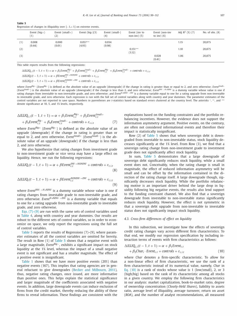
Table 5
Regression of changes in illiquidity over [ −1, + 1] on extreme events.
Event (big + )
(1)
Event (small + )
(2)
Event (big-)(3) Event (small-)
(4)
Event (inv to
non-inv) (5)
Event (non-inv
to inv) (6)
Adj R 2 (%) (7) No. of obs. (8)
(1) 0 .008 0 .0 0 0 0 .057 ∗∗∗ 0 .034 1 .15 20 ,875
(0 .44) (0 .01) (4 .93) (0 .98)
(2) 0 .151 ∗∗∗ 1 .10 20 ,875
(3 .12)
(3) 0 .028 1 .06 20 ,875
(0 .41)
This table reports results from the following regressions:
�I LLI Q c,i ( t − 1 , t + 1 ) = α + β1 Ev ent Big+ c,t + β2 Ev ent Smal l +
c,t + β3 Ev ent Big−c,t + β4 Ev ent Smal l −
c,t + controls + ε c,i,t
�I LLI Q i ( t − 1 , t + 1 ) = α + βEv ent IN V→ N ON IN V c,t + controls + ε c,i,t
�I LLI Q i ( t − 1 , t + 1 ) = α + βEv ent N ON IN V→ IN V c,t + controls + ε c,i,t
where Event Big + ( Event Big −) is defined as the absolute value of an upgrade (downgrade) if the change in rating is greater than or equal to 2, and zero otherwise; Event Small +
( Event Small −) is the absolute value of an upgrade (downgrade) if the change is less than 2, and zero otherwise; Event INV- > N °NINV is a dummy variable whose value is one if
rating changes from investable to non-investable grade, and zero otherwise; and Event N °NINV- > INV is a dummy variable equal to one for a rating upgrade from non-investable
to investable grade, and zero otherwise. Each regression is run with the full set of control variables along with country and year dummies. The parameter estimates of the
control variables are not reported to save space. Numbers in parentheses are t -statistics based on standard errors clustered at the country level. The asterisks ∗ , ∗∗ , and ∗∗∗
denote significance at 10, 5, and 1% levels, respectively.
�
w
u
e
s
2
t
l
�
�
w
r
z
t
g
i
r
o
o
e
T
a
l
e
a
n
e
t
t
a
e
fi
fi
e
b
i
a
i
g
c
s
g
s
e
m
s
r
n
i
u
t
d
r
t
s
4
c
t
t
�
w
a
fi
E
(
i
i
o
r
(
I LLI Q c,i ( t − 1 , t + 1 ) = α + β1 Ev ent Big+ c,t + β2 Ev ent Smal l +
c,t
+ β3 E v ent Big−c,t + β4 E v ent Smal l −
c,t + controls + ε c,i,t (7)
here Event Big + ( Event Big −) is defined as the absolute value of an
pgrade (downgrade) if the change in rating is greater than or
qual to 2, and zero otherwise. Event Small + ( Event Small −) is the ab-
olute value of an upgrade (downgrade) if the change is less than
, and zero otherwise.
We also hypothesize that rating changes from investment grade
o non-investment grade or vice versa may have a large effect on
iquidity. Hence, we run the following regressions:
I LLI Q i ( t − 1 , t + 1 ) = α + βEv ent IN V → N ON IN V c,t + controls + ε c,i,t
(8)
I LLI Q i ( t − 1 , t + 1 ) = α + βEv ent N ON IN V → IN V c,t + controls + ε c,i,t
(9)
here Event INV- > N °NINV is a dummy variable whose value is one if
ating changes from investable grade to non-investable grade, and
ero otherwise. Event N °NINV- > INV is a dummy variable that equals
o one for a rating upgrade from non-investable grade to investable
rade, and zero otherwise.
Eqs. (7)–(9) are run with the same sets of control variables used
n Table 4 , along with country and year dummies. Our results are
obust to the different sets of control variables, so in order to econ-
mize on space, we only report the regressions using the full set
f control variables.
Table 5 reports the results of Regressions (7)–(9), where param-
ter estimates of all the control variables are omitted for brevity.
he result in Row (1) of Table 5 shows that a negative event with
large magnitude, Event Big −, exhibits a significant impact on stock
iquidity at the 1% level, whereas the impact of a small negative
vent is not significant and has a smaller magnitude. The effect of
positive event is insignificant.
Table 1 shows that we have more positive events (201) than
egative events (167). This implies that rating agencies are in gen-
ral reluctant to give downgrades ( Becker and Milbourn, 2011 ),
hus, negative rating changes, once issued, are more informative
han positive ones. This helps explain the statistical significance
nd larger magnitude of the coefficients associated with negative
vents. In addition, large downgrade events can induce exclusion of
rms from the credit market, thereby reducing the ability of these
rms to reveal information. These findings are consistent with the
xplanations based on the funding constraints and the portfolio re-
alancing incentives. However, the evidence does not support the
nformation asymmetry argument. Positive events, on the contrary,
re often not considered informational events and therefore their
mpact is statistically insignificant.
Row (2) of Table 5 shows that when sovereign debt is down-
raded from investable to non-investable status, stock liquidity de-
reases significantly at the 1% level. From Row (3), we find that a
overeign rating change from non-investment grade to investment
rade does not significantly affect stock liquidity.
In sum, Table 5 demonstrates that a large downgrade of
overeign debt significantly reduces stock liquidity, while a small
vent does not. Conceivably, when the rating change is small in
agnitude, the effect of reduced information asymmetry will be
mall and can be offset by the information contained in the di-
ection of the rating change itself. A large downgrade though, sig-
ificantly decreases stock liquidity. While the portfolio rebalanc-
ng motive is an important driver behind the large drop in liq-
idity following big negative events, the results also lend support
o the funding constraint channel. We also find that a sovereign
owngrade from investable to non-investable status significantly
educes stock liquidity. However, the effect is not symmetric in
hat a sovereign debt upgrade from non-investable to investable
tatus does not significantly impact stock liquidity.
.3. Cross-firm differences of effect on liquidity
In this subsection, we investigate how the effects of sovereign
redit rating changes vary across different firm characteristics. To
hat end, we modify our regression specification by including in-
eraction terms of events with firm characteristics as follows:
I LLI Q c,i ( t − 1 , t + 1 ) = α + β1 Ev en t c,t
+ β2 Cha r i · Ev en t c,t + controls + ε c,i,t (10)
here Char denotes a firm-specific characteristic. To allow for
non-linear effect of firm characteristic, we use the rank of a
rm characteristic instead of its numerical value, namely, Char in
q. (10) is a rank of stocks whose value is 1 (low/small), 2, or 3
high/big) based on the rank of its characteristic among all stocks
n a given country. We employ the following firm characteristics
n our analysis: market capitalization, book-to-market ratio, degree
f ownership concentration ( Closely-Held Shares ), liability to assets
atio, average level of illiquidity, average turnover, return on asset
ROA ), and the number of analyst recommendations, all measured

108 K.-H. Lee et al. / Journal of Banking and Finance 73 (2016) 99–112
Table 6
Regression of changes in illiquidity over [ −1, + 1] on events interacted with firm characteristics.
Firm characteristic Event (2) Event Event Event ( + ) Event Event ( −) Adj R 2 No. of
(Char) (1) ∗Char (3) ( + ) (4) ∗Char (5) ( −) (6) ∗Char (7) (%) (8) obs. (9)
(1) Market cap 0 .025 0 .010 1 .14 20 ,875
(0 .81) (0 .61)
0 .007 0 .003 0 .024 0 .014 1 .16 20 ,875
(0 .21) (0 .22) (0 .73) (0 .76)
(2) Book-to-market 0 .033 ∗ 0 .007 1 .14 20 ,875
(1 .72) (1 .17)
−0 .006 0 .011 0 .045 ∗∗ 0 .005 1 .15 20 ,875
(−0 .22) (0 .87) (2 .05) (0 .84)
(3) Closely-held Shares (%) 0 .011 0 .019 ∗∗∗ 1 .41 15 ,710
(0 .61) (2 .98)
−0 .013 0 .007 0 .010 0 .024 ∗∗∗ 1 .45 15 ,710
(−0 .33) (0 .47) (0 .59) (4 .50)
(4) Liability/Assets 0 .069 ∗∗∗ −0 .010 1 .14 20 ,633
(3 .37) (−1 .56)
0 .033 −0 .010 0 .075 ∗∗ −0 .009 1 .16 20 ,633
(1 .14) (−0 .82) (2 .21) (−0 .77)
(5) Illiquidity 0 .0 0 0 0 .025 ∗∗∗ 1 .17 20 ,875
(0 .03) (3 .84)
0 .033 −0 .013 −0 .013 0 .036 ∗∗∗ 1 .22 20 ,875
(1 .33) (−1 .20) (−0 .88) (8 .34)
(6) Turnover 0 .082 ∗∗ −0 .019 0 .97 19 ,810
(2 .19) (−1 .19)
−0 .016 0 .013 0 .121 ∗∗∗ −0 .034 ∗∗ 1 .03 19 ,810
(−0 .53) (0 .98) (3 .09) (−2 .23)
(7) ROA 0 .060 ∗∗ −0 .006 1 .12 19 ,538
(2 .46) (−0 .69)
−0 .004 0 .009 0 .086 ∗∗∗ −0 .015 ∗ 1 .15 19 ,538
(−0 .14) (0 .58) (3 .61) (−1 .82)
(8) N Analyst recommendation 0 .054 ∗∗∗ −0 .006 1 .33 16 ,418
(4 .62) (−0 .65)
0 .015 −0 .003 0 .060 ∗∗∗ −0 .006 1 .34 16 ,418
(0 .38) (−0 .24) (3 .98) (−0 .53)
(9) Politically-connected 0 .048 ∗∗∗ −0 .001 1 .13 20 ,788
(4 .42) (−0 .03)
0 .011 0 .018 0 .056 ∗∗∗ −0 .004 1 .14 20 ,788
(0 .62) (0 .63) (4 .30) (−0 .06)
This table reports results from the following regressions
�I LLI Q c,i ( t − 1 , t + 1 ) = α + β1 Ev en t c,t + β2 Cha r i · Ev en t c,t + controls + ε c,i,t
�I LLI Q c,i ( t − 1 , t + 1 ) = α + β1 Ev ent + c,t + β2 Cha r i · Ev ent + c,t + β3 Ev ent −c,t + β4 Cha r i · Ev ent −c,t + controls + ε c,i,t
Event is the absolute value of a numeric change of sovereign ratings. Event + ( Event −) is the absolute value of a rating change if the change is positive (negative), and zero
otherwise. Char is the rank of a stock, which takes a value of 1(low/small), 2, or 3(high/big) based on the rank of its characteristic among stocks in a given country. The firm
characteristics employed in our analysis include: market capitalization, book-to-market ratio, degree of concentration of ownership ( Closely-Held Shares ), liability to assets
ratio, average illiquidity ( RV ), average turnover, return on asset ( ROA ), and number of analyst recommendations, all measured one year prior to the event. Politically-connected
is a dummy variable equal to 1 if the firm has a political connection and zero otherwise. Each regression is run with the full set of control variables along with country and
year dummies. The parameter estimates of the control variables are not reported to save space. Numbers in parentheses are t -statistics based on standard errors clustered
at the country level. The asterisks ∗ , ∗∗ , and ∗∗∗ denote significance at 10, 5, and 1% levels, respectively.
�
t
a
t
t
i
a
n
t
a
i
d
i
g
c
at the end of the year or over the year prior to the event. We
also distinguish between politically-connected firms from those
that have no political connection, using a dummy variable equal
to one if the firm has a political connection and zero otherwise.
We obtain the list of politically-connected firms used in Faccio
(2006) , and merge that list with our sample firms. We collect the
annual data of closely held shares as percentage of total number
of common shares outstanding from Datastream/Worldscope. The
data on the number of analyst recommendations are from the
I/B/E/S dataset. Each regression is run with the full set of control
variables along with country and year dummies. The parameter
estimates of the control variables are not reported to save space.
Table 6 reports our estimation results. Column (3) shows that
firms with higher degree of ownership concentration or lower liq-
uidity experience a significant liquidity drop from a sovereign debt
rating change.
As shown in the previous sections, downgrades can have a dif-
ferent effect on liquidity than upgrades. Hence, we separate up-
grades (positive events) from downgrades (negative events) and
run the following regression:
iI LLI Q c,i ( t − 1 , t + 1 ) = α + β1 Ev ent + c,t + β2 Cha r i · Ev ent + c,t
+ β3 E v ent −c,t + β4 Cha r i · E v ent −c,t + controls + ε c,i,t (11)
Results reported in Columns (4)–(7) of Table 6 indicate that
he effects of sovereign rating changes interacted with firm char-
cteristics primarily come from downgrades. We find that nega-
ive events interacting with higher degree of ownership concentra-
ion and average illiquidity level significantly reduces stock liquid-
ty. Furthermore, we find negative events interacting with the aver-
ge turnover ratio to be significantly negative at the 5% level, and
egative events interacting with ROA to be significantly negative at
he 10% level.
The results for the negative events interacted with firm char-
cteristics are generally well in accordance with economic intu-
tion. Stocks with a higher fraction of closely-held shares are more
ifficult to rebalance due to shortage of free-floating shares, lead-
ng to more decline in liquidity following a sovereign debt down-
rade. Smaller or more illiquid stocks experience stronger funding
onstraints upon sovereign downgrades, resulting in lower liquid-
ty. Stocks with a higher average turnover ratio face looser funding

K.-H. Lee et al. / Journal of Banking and Finance 73 (2016) 99–112 109
c
i
h
t
a
4
a
t
�
w
c
s
s
l
t
(
(
f
a
v
a
f
k
i
2
a
(
l
o
2
f
a
A
i
a
fi
t
n
s
i
t
l
�
p
s
fi
t
c
u
a
w
h
w
r
t
c
i
b
t
t
t
r
w
t
t
s
4
n
u
s
f
g
a
u
i
u
u
w
[
n
t
a
r
C
e
p
o
c
o
s
5
v
r
T
i
s
a
o
s
w
(
t
w
T
i
b
w
o
m
onstraints following sovereign downgrades, and thus their liquid-
ty will not drop as much. Stocks with a higher return on asset
ave a higher profit margin. They can better handle shocks and
hus following sovereign downgrades, their liquidity will not fall
s much.
.4. Cross-country differences of effect on liquidity
We further explore how the transmission of the externality is
ffected by its interaction with different country characteristics. To
hat end, we run the following regression:
I LLI Q c,i ( t − 1 , t + 1 ) = α + β1 Ev en t c,t
+ β2 CountryV a r i · Ev en t c,t + controls + ε c,i,t (12)
here CountryVar denotes a country-level characteristic. The
ountry-level characteristics that we employ in our analysis are de-
cribed as follows: LAW is a dummy variable equal to one if the
tock is from a civil law country, and zero if it is from a common
aw country; ANTIDIRR is an index of minority investor protec-
ion with a higher value indicating stronger protection; ANTIDIRR
Spamann) is the modified ANTIDIRR index proposed by Spamann
2010) ; EXPRISK is a measure of threat of outright confiscation or
orced nationalization with a higher value indicating a lower risk;
nd ACCSTAND is an index of accounting standard with a higher
alue indicating a higher accounting standard. The above four vari-
bles are previously used in La Porta et al. (1998) . We use the
ollowing additional variables: SCAP is the average of stock mar-
et capitalization to GDP ratio over 1988–1999 ( Stulz, 2005 ); DISCL
s an index of credibility of financial disclosure ( Bushman et al.,
004 ); EARNMGT is an aggregate earnings management score with
higher value indicating a higher level of earnings management
Leuza et al., 2003 ); NANALYSTS is the number of analysts for the
argest 30 firms in a country ( Bushman et al., 2004 ); Foreign inst
wnership is foreign institutional ownership ( Ferreira and Matos,
008 ); and GDP per capita is in 2003 U.S. dollars, which is obtained
rom World Development Indicator.
Each regression is run with the full set of control variables
long with year dummies. Table 7 reports the estimation results.
s can be seen from Column (3), the LAW variable carries a signif-
cant positive sign, indicating that across countries, the impact of
sovereign debt rating changes on stock liquidity is stronger for
rms in a country with civil law than that for firms in a coun-
ry with common law. The coefficient of the DISCL variable is sig-
ificantly negative at the 1% level, implying that the impact of
overeign debt rating changes on stock liquidity is weaker for firms
n a country with higher credibility of financial disclosure.
To investigate differential effects, we separate upgrades (posi-
ive events) from downgrades (negative events) and run the fol-
owing regression:
I LLI Q c,i ( t − 1 , t + 1 ) = α + β1 Ev ent + c,t + β2 Count ryV a r i · Ev ent + c,t
+ β3 E v ent −c,t + β4 CountryV a r i · E v ent −c,t + controls + ε c,i,t (13)
We report results in Columns (4)–(7) of Table 7 . We find the
ositive events interacting with the LAW variable to be statistically
ignificant, implying that following an upgrade in sovereign debt,
rms in a country with civil law will increase liquidity by less than
hose in a country with common law.
The negative coefficients of interaction term with the market
ap variable SCAP shows that the impact of sovereign debt rating
pgrade on stock liquidity is weaker in a country with a larger
verage stock market capitalization. Intuitively, stocks in countries
ith well-developed stock market (as measured by a large SCAP )
ave less liquidity constraint or less information asymmetry.
The significant negative coefficients of the interaction terms
ith the DISCL variable indicate that the impact of sovereign debt
ating changes on stock liquidity is less severe for firms in a coun-
ry with higher credibility of financial disclosure. Intuitively, for a
ountry with high transparency, revision in expectations from new
nformation delivered by rating changes is relatively small either
ecause expectations are less sensitive to new information in a
ransparent environment or because the events add little informa-
ion.
The significant negative coefficient of the interaction term with
he EXPRISK variable suggests that the effect of a sovereign debt
ating changes on stock liquidity is weaker for firms in a country
ith lower risk of outright confiscation or forced nationalization.
Finally, the significant positive coefficient of the interaction
erm with the foreign institutional ownership variable indicates
hat the impact of a sovereign debt downgrade on stock liquidity is
tronger in a country with a higher foreign institutional ownership.
.5. Robustness
In this sub-section, we report more results to check for robust-
ess of our findings. First, we investigate the exposure of stock liq-
idity in each country to a world liquidity factor. In the previous
ections, we have used the global market return, R m, t , to control
or the global factor in all regressions. Lee (2011) finds that an ag-
regate liquidity factor can affect stock returns around the world,
nd it is the U.S. market illiquidity, not the global market illiq-
idity, that significantly impacts individual stock returns. Follow-
ng Lee (2011) , we estimate the daily U.S. market aggregate illiq-
idity by computing an equally-weighted average of stock illiq-
idity (also using the adjusted Amihud measure) in the U.S. and
e use the change of log of (1 + U.S. market illiquidity) over the
–1, + 1] interval. This aggregate market illiquidity measure is de-
oted by �I LLI Q US (t − 1 , t + 1) . We replace the global market re-
urn, R m, t , by the market illiquidity factor, �I LLI Q US (t − 1 , t + 1) ,
nd re-run the previous regressions (5)–(9).
Estimation results are reported in Table 8 . The insignificant pa-
ameters on the changes in the US market illiquidity presented in
olumn (11) show that individual stock liquidity is not significantly
xposed to the U.S. aggregate market liquidity. Comparing with the
revious results reported in Table 4 (Rows (3) and (6)) and Table 5 ,
ur basic conclusions regarding the effects of sovereign debt rating
hanges on stock liquidity remain unchanged.
Second, we check whether our results are robust to the length
f the event window. To that end, we compute the changes in
tock liquidity over the longer event windows of [–2, + 2] and [–
, + 5]. We run Regressions (5) and (6) with various sets of control
ariables with this longer event window and report the estimation
esults in Table 9.
Panel A of Table 9 shows similar results to those reported in
able 4 . That is, the coefficients on Event and Event − are all signif-
cant at the 1% level, though the magnitude and the t -values are
maller than those in Table 4 , even when all the control variables
re included.
Rows (1)–(2) of panel B of Table 9 show that the coefficient
f the Event variable is positive and statistically significant, con-
istent with those in our baseline case reported in Table 4 , only
hen other firm-level control variables are not included. In rows
3)-(4) of panel B, we also find that the coefficient of the posi-
ive events and negative events is significant at the 10% level only
hen firm-level control variables are excluded in the regressions.
hese results are in general weaker than those reported in Table 4 ,
mplying that the impact of sovereign rating changes are absorbed
y the market rather quickly.
For further robustness check, we repeat all regressions only
ith the change in illiquidity over the day of the rating change, i.e.,
ver [–1,0]. If a rating change itself is an informational event that
ay reduce information asymmetry, liquidity may improve right

110 K.-H. Lee et al. / Journal of Banking and Finance 73 (2016) 99–112
Table 7
Regression of change in illiquidity over [ −1, + 1] on events interacted with country-specific variables.
Country specific Event (2) Event ∗ Event Event ( + ) ∗ Event Event ( −) ∗ No. of Adj R 2
variable (CV) (1) CV (3) ( + ) (4) CV (5) ( −) (6) CV (7) obs. (8) (%) (9)
(1) LAW −0 .088 ∗ 0 .140 ∗∗ 19 ,831 0 .75
(0 = common, 1 = civil law) (−1 .70) (2 .67)
−0 .116 ∗∗ 0 .129 ∗∗ 0 .006 0 .056 19 ,831 0 .83
(−2 .28) (2 .40) (0 .06) (0 .61)
(2) ANTIDIRR 0 .080 ∗ −0 .014 19 ,825 0 .74
(1 .82) (−0 .82)
0 .034 −0 .016 0 .107 ∗∗ −0 .021 19 ,825 0 .79
(0 .71) (−0 .85) (2 .07) (−1 .00)
(3) ANTIDIRR −0 .121 0 .040 19 ,825 0 .68
(Spamann) (−0 .74) (0 .97)
−0 .029 0 .006 −0 .029 0 .020 19 ,825 0 .71
(−0 .18) (0 .15) (−0 .13) (0 .36)
(4) EXPRISK 0 .247 −0 .024 19 ,831 0 .73
(1 .59) (−1 .33)
0 .315 ∗ −0 .038 ∗ 0 .427 ∗∗ −0 .044 ∗ 19 ,831 0 .79
(1 .94) (−1 .95) (1 .96) (−1 .77)
(5) ACCSTAND 0 .220 −0 .003 19 ,751 0 .71
(1 .16) (−0 .94)
0 .244 −0 .004 0 .412 −0 .006 19 ,751 0 .79
(1 .44) (−1 .48) (1 .38) (−1 .21)
(6) SCAP 0 .083 ∗∗∗ −0 .080 19 ,291 0 .75
(2 .71) (−1 .31)
0 .047 −0 .112 ∗ 0 .109 ∗∗∗ −0 .114 19 ,291 0 .81
(1 .52) (−1 .75) (2 .81) (−1 .52)
(7) DISCL 0 .217 ∗∗∗ −0 .002 ∗∗∗ 19 ,827 0 .82
(3 .68) (−2 .85)
0 .190 ∗∗ −0 .003 ∗∗ 0 .286 ∗∗∗ −0 .003 ∗∗∗ 19 ,827 0 .87
(2 .42) (−2 .30) (3 .71) (−3 .01)
(8) EARNMGT −0 .062 0 .004 17 ,728 0 .71
(−0 .83) (1 .46)
−0 .107 0 .004 −0 .069 0 .005 17 ,728 0 .75
(−1 .40) (1 .50) (−0 .58) (1 .02)
(9) NANALYSTS 0 .007 0 .004 19 ,827 0 .69
(0 .09) (0 .51)
−0 .023 0 .002 0 .062 −0 .001 19 ,827 0 .73
(−0 .29) (0 .30) (0 .65) (−0 .09)
(10) Foreign inst ownership −0 .098 0 .012 14 ,719 0 .56
(% of market cap) (−1 .27) (1 .52)
−0 .051 0 .007 −0 .182 ∗∗ 0 .022 ∗∗ 14 ,719 0 .58
(−0 .38) (0 .54) (−2 .00) (2 .05)
(11) GDP per capita (in 2003 U.S. dollars) 0 .038 0 .0 0 0 21 ,071 0 .74
(1 .10) (−0 .24)
0 .0 0 0 0 .0 0 0 0 .063 0 .0 0 0 21 ,071 0 .78
(−0 .00) (−0 .45) (1 .56) (−0 .77)
This table reports results from the following regressions:
�I LLI Q c,i ( t − 1 , t + 1 ) = α + β1 Ev en t c,t + β2 CountryVa r i · Ev en t c,t + controls + ε c,i,t
�I LLI Q c,i ( t − 1 , t + 1 ) = α + β1 Ev ent + c,t + β2 Count ryVa r i · Ev ent + c,t + β3 Ev ent −c,t + β4 Count ryVa r i · Ev ent −c,t + cont rols + ε c,i,t
where Event is the absolute value of a numeric change of sovereign ratings; Event + ( Event −) is the absolute value of a rating change if the change is positive (negative), and
zero otherwise; LAW is a dummy variable equal to one if the stock is from a civil law country, and zero if it is from a common law country; ANTIDIRR is an index of minority
investor protection with a higher value indicating stronger protection; EXPRISK is a measure of political risk with a higher value indicating a lower risk; ACCSTAND is an index
of accounting standard with a higher value indicating a higher accounting standard; SCAP is the average of stock market capitalization to GDP ratio over 1988–1999; DISCL is
an index of accounting standard; EARNMGT is an aggregate earnings management score with a higher value indicating a higher level of earnings management; NANALYSTS is
the number of analysts covered for the largest 30 firms in a country; Foreign inst ownership is foreign institutional ownership; and GDP per capita is in 2003 U.S. dollars. Each
regression is run with the full set of control variables along with year dummies. The parameter estimates of the control variables are not reported to save space. Numbers
in parentheses are t -statistics based on standard errors clustered at the country level. The asterisks ∗ , ∗∗ , and ∗∗∗ denote significance at 10, 5, and 1% levels, respectively.
t
t
g
c
5
p
4
r
c
after the announcement is made, so that the change can be cap-
tured by the window of [–1,0]. We find that the Event and Event
(–) variables are generally insignificant except for the case when
the full set of control variables are used, the case in which they
are negative and significant only at the 10% level. With such weak
evidence for [–1,0], it is difficult to draw a solid conclusion that
the announcement itself is an informational event, These result are
also not reported to save space.
As we revealed in the footnote in Section 3 , our results remain
robust when we use $2 cutoff price to screen the sample.
Lastly, and maybe most importantly, we performed all the anal-
yses with the original Amihud measure with fitted values from
both the regressions of stock return on dollar volume and on
uurnover volume. We also repeated all the analyses based on
urnover-based Amihud measure with fitted values from the re-
ression of return on dollar volume. Our results are similar in all
ases.
. Conclusion
Sovereign rating changes affect stock liquidity. We examine the
resence of such externality using data for a panel of stocks from
0 countries over the last two decades and find that sovereign
ating changes have a significant impact on stock liquidity. Large
hanges in sovereign ratings have stronger effects on equity liq-
idity than small changes. Furthermore, the effect is asymmetric,

K.-H. Lee et al. / Journal of Banking and Finance 73 (2016) 99–112 111
Table 8
Regression of changes in illiquidity over [ −1, + 1] on events after controlling for U.S. market liquidity.
Intercept Event Event Event Event Event Event Event Event (inv Event (noninv �ILLIQ US log log Stdev logRV Adj No. of
( + ) ( −) (big + ) (big-) (small + ) (small-) to noninv) to inv) (MV) (B/M) R 2 (%) obs.
(1) (2) (3) (4) (5) (6) (7) (8) (9) (10) (11) (12) (13) (14) (15) (16) (17)
(1) −0 .149 ∗∗ 0 .052 ∗∗∗ −0 .007 0 .007 ∗∗∗ 0 .005 1 .449 ∗∗∗ −0 .018 1 .00 19 ,869
(−2 .11) (3 .65) (−0 .03) (2 .65) (0 .72) (2 .96) (−1 .27)
(2) −0 .146 ∗∗ 0 .017 0 .059 ∗∗∗ 0 .028 0 .007 ∗∗ 0 .004 1 .369 ∗∗∗ −0 .018 1 .02 19 ,869
(−2 .01) (0 .79) (3 .81) (0 .13) (2 .40) (0 .63) (2 .69) (−1 .27)
(3) −0 .145 ∗∗ 0 .004 0 .062 ∗∗∗ 0 .021 0 .046 0 .045 0 .007 ∗∗ 0 .004 1 .347 ∗∗∗ −0 .017 1 .02 19 ,869
(−2 .02) (0 .21) (4 .85) (0 .37) (0 .91) (0 .18) (2 .41) (0 .64) (2 .63) (−1 .24)
(4) −0 .144 ∗∗ 0 .149 ∗∗∗ 0 .084 0 .008 ∗∗∗ 0 .005 1 .635 ∗∗∗ –0.017 0 .96 19 ,869
(−1 .97) (2 .64) (0 .50) (2 .69) (0 .78) (3 .62) (−1 .20)
(5) −0 .137 ∗ 0 .049 0 .227 0 .008 ∗∗∗ 0 .005 1 .740 ∗∗∗ −0 .017 0 .92 19 ,869
(−1 .95) (0 .70) (1 .22) (2 .76) (0 .80) (3 .63) (−1 .20)
This table reports results from the following regressions:
�I LLI Q c,i ( t − 1 , t + 1 ) = α + β1 Ev en t c,t + β2 �I LLI Q US (t − 1 , t + 1) + β3 log (MV ) i,y −1 + β4 log (B/M) i,y −1 + β5 St de v i,t −30 ,t −1 + β6 log R V i,y −1 + other cont rols + ε c,i,t
�I LLI Q c,i ( t − 1 , t + 1 ) = α + β1 Ev ent + c,t + β2 Ev ent −c,t + controls + ε c,i,t
�I LLI Q c,i ( t − 1 , t + 1 ) = α + β1 Ev ent Big+ c,t + β2 Ev ent Smal l +
c,t + β3 Ev ent Big−c,t + β4 Ev ent Smal l −
c,t + controls + ε c,i,t
�I LLI Q i ( t − 1 , t + 1 ) = α + β Ev ent IN V→ N ON IN V c,t + controls + ε c,i,t
�I LLI Q i ( t − 1 , t + 1 ) = α + β Ev ent N ON IN V→ IN V c,t + controls + ε c,i,t ,
�I LLI Q US (t − 1 , t + 1) is the change in U.S. market liquidity, and all other variables are defined the same way as in the previous tables. Each regression also contains country
and year dummies. Numbers in parentheses are t -statistics based on standard errors clustered at the country level. The asterisks ∗ , ∗∗ , and ∗∗∗ denote significance at 10, 5,
and 1% levels, respectively.
Table 9
Regression of changes in illiquidity over [ −5, + 5] on events.
Intercept Event Event ( + ) Event ( −) Global market log(MV) log(B/M) Stdev logRV Adj R 2 (%) No. of obs.
return, R m
Panel A. Event windows of [ −2, + 2]
(1) −0 .086 ∗ 0 .048 ∗∗∗ 0 .128 0 .746 20 ,387
(−1 .70) (2 .85) (0 .21)
(2) −0 .091 0 .040 ∗∗ 0 .164 −0 .002 −0 .011 0 .908 ∗∗ −0 .021 0 .840 20 ,207
(−1 .33) (2 .34) (0 .26) (−0 .62) (−1 .02) (2 .47) (−1 .17)
(3) −0 .083 ∗ 0 .022 0 .053 ∗∗∗ 0 .125 0 .755 20 ,387
(−1 .69) (0 .64) (3 .23) (0 .20)
(4) −0 .085 0 .016 0 .045 ∗∗ 0 .160 −0 .003 −0 .011 0 .861 ∗∗ −0 .021 0 .847 20 ,207
(−1 .28) (0 .48) (2 .60) (0 .25) (−0 .75) (−1 .05) (2 .39) (−1 .18)
Panel B. Event windows of [ −5, + 5]
(1) 0 .169 ∗∗∗ 0 .061 ∗∗ −0 .104 0 .894 19 ,502
(2 .99) (2 .13) (−0 .36)
(2) 0 .206 ∗∗∗ 0 .045 −0 .060 −0 .011 ∗ −0 .007 1 .164 ∗∗ 0 .001 0 .942 19 ,344
(3 .08) (1 .59) (−0 .21) (−1 .94) (−0 .67) (2 .47) (0 .04)
(3) 0 .169 ∗∗∗ 0 .068 ∗ 0 .058 ∗ −0 .096 0 .890 19 ,502
(2 .97) (1 .91) (1 .86) (−0 .35)
(4) 0 .206 ∗∗∗ 0 .046 0 .045 −0 .059 −0 .011 ∗ −0 .007 1 .165 ∗∗ 0 .001 0 .937 19 ,344
(3 .07) (1 .23) (1 .57) (−0 .22) (−1 .96) (−0 .67) (2 .57) (0 .04)
This table reports results from the following regressions:
�I LLI Q c,i ( t − k, t + k ) = α + β1 Ev en t c,t + controls + ε c,i,t
�I LLI Q c,i ( t − k, t + k ) = α + β1 Ev ent + c,t + β2 Ev ent −c,t + controls + ε c,i,t ,
�I LLI Q c,i ( t − k, t + k ) is the change in liquidity for stock i over the [t-k,t + k] interval and all other variables are defined the same way as in the previous tables. Each regression
also contains country and year dummies. Numbers in parentheses are t -statistics based on standard errors clustered at the country level. The asterisks ∗ , ∗∗ , and ∗∗∗ denote
significance at 10, 5, and 1% levels, respectively.
i
u
p
fi
t
r
r
s
f
d
m
f
t
d
s
s
n
h
c
i
a
c
d
n that the impact is much stronger for downgrades than for
pgrades. The loss of sovereign investment grade status has a
articularly strong negative impact on stock liquidity. Overall, our
ndings lend support to the funding constraints hypothesis in
hat a binding funding constraint, which is triggered by sovereign
ating downgrade, is the channel through which the unfavorable
ating changes lead to deterioration in stock liquidity. These re-
ults are robust after controlling for country- and firm-specific
actors.
In focusing on the implications of changes in public debt con-
itions on stock liquidity, our study highlights an additional trans-
ission channel through which the management of public debt af-
ects the private sector. In addition, our work explores how the
ransmission of the externality is affected by its interaction with
ifferent firm-level and country-specific characteristics.
At the firm level, we find that in response to a negative
overeign credit event, firms with higher concentration of owner-
hip or lower liquidity level tend to experience more significant
egative liquidity effects, while firms with higher turnover ratio or
igher return on assets tend to experience significantly smaller de-
reases in stock liquidity following a sovereign downgrade.
At the country level, on the one hand, higher stock market cap-
talization relative to GDP, higher credibility of financial disclosure,
nd lower risk of outright confiscation or forced nationalization are
ountry-level factors that lessen the impact of a sovereign debt
owngrade on stock liquidity. On the other hand, civil law origin
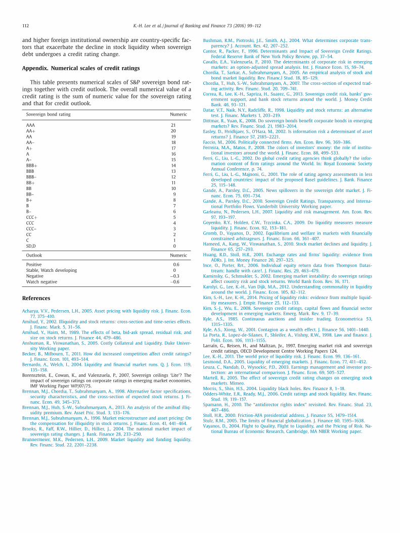
112 K.-H. Lee et al. / Journal of Banking and Finance 73 (2016) 99–112
B
C
C
C
C
C
D
D
E
F
F
F
G
G
G
G
G
H
I
K
K
K
K
L
M
S
S
V
and higher foreign institutional ownership are country-specific fac-
tors that exacerbate the decline in stock liquidity when sovereign
debt undergoes a credit rating change.
Appendix. Numerical scales of credit ratings
This table presents numerical scales of S&P sovereign bond rat-
ings together with credit outlook. The overall numerical value of a
credit rating is the sum of numeric value for the sovereign rating
and that for credit outlook.
Sovereign bond rating Numeric
AAA 21
AA + 20
AA 19
AA– 18
A + 17
A 16
A– 15
BBB + 14
BBB 13
BBB– 12
BB + 11
BB 10
BB– 9
B + 8
B 7
B– 6
CCC + 5
CCC 4
CCC– 3
CC 2
C 1
SD,D 0
Outlook Numeric
Positive 0 .6
Stable, Watch developing 0
Negative −0 .3
Watch negative −0 .6
References
Acharya, V.V. , Pedersen, L.H. , 2005. Asset pricing with liquidity risk. J. Financ. Econ.
77, 375–410 . Amihud, Y. , 2002. Illiquidity and stock returns: cross-section and time-series effects.
J. Financ. Mark. 5, 31–56 . Amihud, Y. , Haim, M. , 1989. The effects of beta, bid-ask spread, residual risk, and
size on stock returns. J. Finance 44, 479–486 .
Anshuman, R. , Viswanathan, S. , 2005. Costly Collateral and Liquidity. Duke Univer-sity Working paper .
Becker, B. , Milbourn, T. , 2011. How did increased competition affect credit ratings?J. Financ. Econ. 101, 493–514 .
Bernardo, A. , Welch, I. , 2004. Liquidity and financial market runs. Q. J. Econ. 119,135–158 .
Borensztein, E., Cowan, K., and Valenzuela, P., 2007, Sovereign ceilings ‘Lite’? The
impact of sovereign ratings on corporate ratings in emerging market economies,IMF Working Paper WP/07/75.
Brennan, M.J. , Chordia, T. , Subrahmanyam, A. , 1998. Alternative factor specifications,security characteristics, and the cross-section of expected stock returns. J. Fi-
nanc. Econ. 49, 345–373 . Brennan, M.J. , Huh, S.-W. , Subrahmanyam, A. , 2013. An analysis of the amihud illiq-
uidity premium. Rev. Asset Pric. Stud. 3, 133–176 .
Brennan, M.J. , Subrahmanyam, A. , 1996. Market microstructure and asset pricing: Onthe compensation for illiquidity in stock returns. J. Financ. Econ. 41, 441–464 .
Brooks, R. , Faff, R.W. , Hillier, D. , Hillier, J. , 2004. The national market impact ofsovereign rating changes. J. Bank. Finance 28, 233–250 .
Brunnermeier, M.K. , Pedersen, L.H. , 2009. Market liquidity and funding liquidity.Rev. Financ. Stud. 22, 2201–2238 .
ushman, R.M. , Piotroski, J.E. , Smith, A.J. , 2004. What determines corporate trans-parency? J. Account. Res. 42, 207–252 .
antor, R. , Packer, F. , 1996. Determinants and Impact of Sovereign Credit Ratings.Federal Reserve Bank of New York Policy Review, pp. 37–54 .
avallo, E.A. , Valenzuela, P. , 2010. The determinants of corporate risk in emergingmarkets: an option-adjusted spread analysis. Int. J. Finance Econ. 15, 59–74 .
hordia, T. , Sarkar, A. , Subrahmanyam, A. , 2005. An empirical analysis of stock andbond market liquidity. Rev. Financ.l Stud. 18, 85–129 .
hordia, T. , Huh, S.-W. , Subrahmanyam, A. , 2007. The cross-section of expected trad-
ing activity. Rev. Financ. Stud. 20, 709–741 . orrea, R. , Lee, K.-H. , Sapriza, H. , Suarez, G. , 2013. Sovereign credit risk, banks’ gov-
ernment support, and bank stock returns around the world. J. Money CreditBank. 46, 93–121 .
atar, V.T. , Naik, N.Y. , Radcliffe, R. , 1998. Liquidity and stock returns: an alternativetest. J. Financ. Markets 1, 203–219 .
ittmar, R. , Yuan, K. , 2008. Do sovereign bonds benefit corporate bonds in emerging
markets? Rev. Financ. Stud. 21, 1983–2014 . asley, D. , Hvidkjaer, S. , O’Hara, M. , 2002. Is information risk a determinant of asset
returns? J. Finance 57, 2185–2221 . accio, M. , 2006. Politically connected firms. Am. Econ. Rev. 96, 369–386 .
erreira, M.A. , Matos, P. , 2008. The colors of investors’ money: the role of institu-tional investors around the world. J. Financ. Econ. 88, 499–533 .
erri, G. , Liu, L.-G. , 2002. Do global credit rating agencies think globally? the infor-
mation content of firm ratings around the World. In: Royal Economic SocietyAnnual Conference, p. 74 .
Ferri, G. , Liu, L.-G. , Majnoni, G. , 2001. The role of rating agency assessments in lessdeveloped countries: impact of the proposed Basel guidelines. J. Bank. Finance
25, 115–148 . ande, A. , Parsley, D.C. , 2005. News spillovers in the sovereign debt market. J. Fi-
nanc. Econ. 75, 691–734 .
ande, A. , Parsley, D.C. , 2010. Sovereign Credit Ratings, Transparency, and Interna-tional Portfolio Flows. Vanderbilt University Working paper .
arleanu, N. , Pedersen, L.H. , 2007. Liquidity and risk management. Am. Econ. Rev.97, 193–197 .
oyenko, R.Y. , Holden, C.W. , Trzcinka, C.A. , 2009. Do liquidity measures measureliquidity. J. Financ. Econ. 92, 153–181 .
romb, D. , Vayanos, D. , 2002. Equilibrium and welfare in markets with financially
constrained arbitrageurs. J. Financ. Econ. 66, 361–407 . ameed, A. , Kang, W. , Viswanathan, S. , 2010. Stock market declines and liquidity. J.
Finance 65, 257–293 . Huang, R.D. , Stoll, H.R. , 2001. Exchange rates and firms’ liquidity: evidence from
ADRs. J. Int. Money Finance 20, 297–325 . nce, O. , Porter, Rrt. , 2006. Individual equity return data from Thompson Datas-
tream: handle with care!. J. Financ. Res. 29, 463–479 .
aminsky, G. , Schmukler, S. , 2002. Emerging market instability: do sovereign ratingsaffect country risk and stock returns. World Bank Econ. Rev. 16, 171 .
arolyi, G. , Lee, K.-H. , Van Dijk, M.A. , 2012. Understanding commonality in liquidityaround the world. J. Financ. Econ. 105, 82–112 .
Kim, S.-H. , Lee, K.-H. , 2014. Pricing of liquidity risks: evidence from multiple liquid-ity measures. J. Empir. Finance 25, 112–133 .
im, S.-J. , Wu, E. , 2008. Sovereign credit ratings, capital flows and financial sectordevelopment in emerging markets. Emerg. Mark. Rev. 9, 17–39 .
Kyle, A.S. , 1985. Continuous auctions and insider trading. Econometrica 53,
1315–1335 . yle, A.S. , Xiong, W. , 2001. Contagion as a wealth effect. J. Finance 56, 1401–1440 .
La Porta, R. , Lopez-de-Silanes, F. , Shleifer, A. , Vishny, R.W. , 1998. Law and finance. J.Polit. Econ. 106, 1113–1155 .
Larraín, G., Reisen, H., and Maltzan, Jv., 1997, Emerging market risk and sovereigncredit ratings, OECD Development Centre Working Papers 124.
ee, K.-H. , 2011. The world price of liquidity risk. J. Financ. Econ. 99, 136–161 .
Lesmond, D.A. , 2005. Liquidity of emerging markets. J. Financ. Econ. 77, 411–452 . Leuza, C. , Nandab, D. , Wysockic, P.D. , 2003. Earnings management and investor pro-
tection: an international comparison. J. Financ. Econ. 69, 505–527 . artell, R. , 2005. The effect of sovereign credit rating changes on emerging stock
markets. Mimeo . Morris, S. , Shin, H.S. , 2004. Liquidity black holes. Rev. Finance 8, 1–18 .
Odders-White, E.R. , Ready, M.J. , 2006. Credit ratings and stock liquidity. Rev. Financ.
Stud. 19, 119–157 . pamann, H. , 2010. The “antidirector rights index” revisited. Rev. Financ. Stud. 23,
467–486 . toll, H.R. , 20 0 0. Friction-AFA presidential address. J. Finance 55, 1479–1514 .
Stulz, R.M. , 2005. The limits of financial globalization. J. Finance 60, 1595–1638 . ayanos, D. , 2004. Flight to Quality, Flight to Liquidity, and the Pricing of Risk. Na-
tional Bureau of Economic Research, Cambridge, MA NBER Working paper .