Journal of Computer and System Sciences 89 (2017) 190–208

Contents lists available at ScienceDirect

Journal of Computer and System Sciences

www.elsevier.com/locate/jcss

Zigzag Decodable codes: Linear-time erasure codes

with applications to data storage

Xueqing Gong ∗, Chi Wan Sung

a r t i c l e i n f o a b s t r a c t

Article history:Received 6 May 2016Received in revised form 4 January 2017Accepted 9 May 2017Available online 24 May 2017

Keywords:Zigzag Decodable codesk-ReliabilityErasure codesData storageLinear timeImplementation

An erasure code is said to be k-reliable if it maps k source packets into n coded packets, and any k out of the n coded packets allow recovery of the original k source packets. Codes of k-reliability achieve the best reliability-storage tradeoff, which are useful for fault tolerance in data storage systems. Zigzag Decodable (ZD) codes are k-reliable erasure codes. Its encoding and decoding (per information bit) can be done in linear time, involving only XOR and bit-shift operations. Two classes of ZD codes are constructed, and compared with Cacuhy-RS codes, the state-of-the-art general-purpose MDS codes. Numerical results show that ZD codes outperform Cauchy-RS codes over a wide range of coding parameters.

© 2017 Elsevier Inc. All rights reserved.

1. Introduction

Due to the explosive growth of personal and enterprise digital data, providing good data storage solutions becomes a popular topic. To design a data storage system, high reliability is very important, since no one wants to experience data loss. The simplest way to provide reliability is to replicate the data multiple times and store them into independent storage devices, which can be multiple hard disks or data servers located in geographically separated areas. From the perspective of coding theory, this simple solution corresponds to the use of repetition codes, which is well known to be inefficient in terms of storage space. To improve storage efficiency, one may use erasure codes, which can achieve the same level of reliability with much less redundancy. On the other hand, the use of erasure codes requires the calculation of parity bits when storing a file into the system, and the calculation of information bits when the file is retrieved by assessing storage devices that have stored the parity bits. These operations not only increase the response times of storing and retrieving a file from the storage system, but also consumes more energy due to the computations. As for traditional erasure codes, the encoding and decoding often involve multiplication over a large finite field, which is much more time and energy consuming than addition [1]. For many applications, such as big-data storage systems and mobile systems with hand-held devices that have low computation capability [2], it is important to have a storage system that can provide high accessibility and low energy consumption for both storage and retrieval. Therefore, it is useful to design erasure codes that have low encoding and decoding complexities.

Erasure codes have been adopted in data storage systems such as Oceanstore, Total Recall systems, and Windows Azure Storage. The most important group of erasure codes are Maximum Distance Separable (MDS) codes, which are optimal in terms of storage efficiency. According to the classification in [3], existing MDS codes for data storage can be categorized

* Corresponding author.E-mail address: xgong6-c@my.cityu.edu.hk (X. Gong).

http://dx.doi.org/10.1016/j.jcss.2017.05.0050022-0000/© 2017 Elsevier Inc. All rights reserved.

X. Gong, C.W. Sung / Journal of Computer and System Sciences 89 (2017) 190–208 191

into two groups. One is called general-purpose codes, which can tolerate any pre-specified number of failures. The other is called special-purpose codes, which can tolerate exactly a certain number of failures, typically two or three.

With regard to special-purpose codes, a noteworthy example is the redundant array of inexpensive disk (RAID) system, which uses multiple disks as a single logical storage unit for fault tolerance. EVENODD [4], RDP codes [5] X-code [6], and Minimal Density RAID-6 codes [7,8] are specially designed for RAID-6, which is required to tolerate double disk failures. Besides, there are also codes specially designed for tolerating triple disk failures [9–14]. A new MDS array code is designed in [15], which can tolerate five disk failures.

Comparatively, general-purpose codes are more flexible, as they provide a wider range of coding parameters such as code rate and the maximum number of tolerable failures. To describe these codes, we use n, k, and L to denote the number of encoded packets, the number of source packets and the size of each source packet, respectively.

The most representative class of general-purpose codes is Reed–Solomon (RS) codes introduced in [16], which have encoding and decoding time complexity of O (n log2 n log log n) [17, Chapter 11.7]. As the codes are defined over a large finite field, encoding and decoding operations are computationally expensive, which prevents it from being widely used in practical data storage systems. Another class of general-purpose MDS codes is proposed in [18], which has a decoding complexity of O (k4L3). However, the decoding complexity is cubic in terms of the packet size L, which is usually a large number in data storage systems. In [19], Blaum et al. construct a family of MDS array codes aiming to tolerate multiple disk failures, while they only provide efficient encoding and decoding procedures for the case of two or three disk failures. Its decoding complexity for general cases increases exponentially with the number of erasures. There is another class of stan-dard general-purpose erasure codes, low-density parity-check (LDPC) codes, which achieve attractive decoding performance. Plank and Thomason investigate the application of LDPC codes in data storage systems in [20]. Their experiment results show that LDPC codes achieve good performance only when k is large. Reed–Solomon codes clearly outperform LDPC codes when k ≤ 36. Digital fountain codes, such as LT codes, also have been studied [21–23]. To apply LT codes to data storage, the challenge is that there is a small probability that a user may not be able to recover the original data from any k sur-vived data packets. Cao et al. proposed an LT-code-based secure cloud storage service (LTCS) in [24]. Exhaustive search is used to obtain a feasible code instance. Though the decoding complexity of LTCS is as low as LT codes, which is nearly O (k ln k), the exhaustive search method is time consuming and sometimes not even be able to output a valid LT code. As it is too complicated to estimate the time of obtaining a valid LT code for a specified storage system, we do not compare the performance of our proposed codes with LT codes in this paper. Cauchy-RS codes are another class of general-purpose MDS codes [25], which improves the RS codes with two modifications. First, the generator matrix becomes the Cauchy matrix instead of the Vandermonde matrix. Second, multiplication in finite field is replaced by the exclusive-or (XOR) operation. The decoding complexity of Cauchy-RS codes is O (kωL), where ω is the word size. Its performance can be further improved by optimizing the Cauchy distribution matrix [26]. As Cauchy-RS codes are widely accepted as good general-purpose MDS codes, we use it as the benchmark for evaluating the performance of our proposed codes.

In this paper, we propose a new class of general-purpose erasure codes based on the concept of zigzag decoding [27]. The encoding and decoding process of ZD codes involve only the bit-shift and XOR operations. Decoding is done by zigzag decoding, with time complexity of O (k2L) or equivalently O (kM), where M is the total number of information bits. In other words, the time complexity per information bit is O (k). As no finite-field multiplication is needed and the decoding complexity per information bit in terms of XOR is linear, decoding is very fast. We focus only on time complexity. Space complexity of decoding ZD codes is considered in [28].

This paper is an extension of our preliminary work in [29]. It provides a much more comprehensive treatment on ZD codes. Our contributions are summarized as follows:

• We provide a detailed, rigorous proof of an essential condition called increasing-difference property for constructing feasible ZD codes. Two feasible constructions for ZD codes are proposed. One is Vandermonde-matrix based ZD codes and the other is Hankel-matrix based ZD codes.

• We compare the encoding and decoding performance of RDP codes, Cauchy-RS codes and ZD codes by both mathemat-ical analysis and software implementation. As the Jerasure library in [30] implements the fastest version of Cauchy-RS codes, we employ this library to obtain the performance of Cauchy-RS codes. We conduct extensive experiments on encoding and decoding performance evaluation of the three codes. We not only compare their performance under or-dinary settings of storage systems, but also investigate the potential and restriction of ZD codes in a wide variety of scenarios. Our experimental results show that ZD codes outperform Cauchy-RS codes in most scenarios.

• We compare the storage overhead of the two different ZD code constructions. Under the ordinary settings of practical storage systems, the storage overhead required of Hankel-matrix based ZD codes is less than 0.7% of the total storage amount of the system and is much smaller than the overhead of Vandermonde-matrix based ZD codes.

The rest of this paper is organized as follows. In section 2, we provide a short introduction of the zigzag decoding concept. In Section 3, we briefly review the ideas of RDP codes and Cauchy-RS codes. In Section 4, we explain the idea of ZD codes and the two construction methods. In Section 5, we present the details of implementation and the parameter settings. In Section 6, we analyze the computational complexities of the encoding and decoding algorithms of the three codes. In Section 7, we provide numerical results and performance evaluation of different coding schemes. Section 8 concludes our paper.

192 X. Gong, C.W. Sung / Journal of Computer and System Sciences 89 (2017) 190–208

Fig. 1. Example of zigzag decoding.

2. Related work on zigzag decoding

The zigzag decoding concept is first introduced in [27] to combat the hidden terminal problem in wireless networks. As shown in Fig. 1, x and y are source packets sent by two senders who are unable to sense each other. Let p1 and p2be two received packets obtained by the superpositions of two “collided” packets with different offsets. The first bit x1is interference-free in p1, so it can be directly read out. After subtracting x1 from p2, y1 can be obtained. Repeat this process until every bit of x and y is decoded. The access to the two collision packets follows a zigzag pattern. In this scenario, the maximum number of overlapped source packets to perform zigzag decoding is two. Similar to the idea of zigzag decoding, a triangular network coding scheme was proposed for the wireless broadcasting problem in [31], with an aim of obtaining more innovative encoding packets. The concept of shift operations are also employed to design packet-level forward error correcting codes in [32], but their decoding process is based on matrix inversion, which is different from the zigzag decoding algorithm in this paper. Besides, the same idea of introducing extra overhead to parity packets can also be found in the construction of a regenerating code in [33].

The idea of zigzag decoding can be applied to the design of general-purpose erasure codes. Motivated by the low time complexity of zigzag decoding, we design the first class of zigzag decodable (ZD) codes in [29]. Our designed codes have the same erasure fault tolerance capability as MDS codes, but strictly speaking, they are not MDS codes due to the extra overhead incurred by the bit-shift operation to be described in Section 4. To avoid misunderstanding, we define the notion of k-reliability, which can be used to describe the erasure fault tolerance of both ZD codes and MDS codes:

Definition 1. An (n, k) code is said to be k-reliable if after encoding k information symbols into n coded symbols, the kinformation symbols can be recovered by any k of the coded symbols.

ZD codes have been applied to various situations. For example, they can be used as a network coding scheme for the combination network [34]. Besides, a fountain code based on ZD codes is proposed in [35] and is shown to outperform Raptor codes in terms of the transmissions overhead. Since ZD codes are general-purpose erasure codes, in principle, they can be used in any scenario which uses existing erasure codes as one of the building components. An example is the STAIR code, which is recently proposed for tolerating device and sector failures in practical storage systems [36].

Apart from pursuing excellent encoding and decoding performance for data retrieval problems, how to repair failed nodes is also an important issue in maintaining the reliability of data storage systems. Repairing schemes for single-failure cases of RDP and EVENODD codes are proposed in [37,38]. Zhu et al. proposed an efficient repair algorithm for single-node failure for general MDS array codes in [39]. Hou et al. proposed the BASIC code for both functional repair and exact repair [40]. In this paper, we focus on the encoding and decoding speeds of the data storage and retrieval processes. We remark that ZD codes can be used as the outer code of the Fractional Repetition codes, which support exact and uncoded repair [41,42]. Designing ZD codes with efficient repair property is an interesting topic for future work.

3. MDS codes for data storage systems

The MDS codes are known to be optimal in terms of reliability-redundancy tradeoff. A comprehensive performance comparison among different MDS codes is made in [3]. Based on their evaluation, the encoding and decoding performance of RDP outperforms other codes when the number of parity symbols is two. As the other special-purpose erasure codes such as STAR codes [43] and generalized EVENODD codes are very similar to RDP codes, while our proposed codes are designed for tolerating multiple failures, we treat RDP as a representative of special-purpose codes and use it as a benchmark for comparison.

For general-purpose codes, as discussed in the previous section, Cauchy-RS codes are the most efficient general-purpose erasure codes. Therefore, we studied in detail the performance comparison between ZD codes and Cauchy-RS codes. The performance of Cauchy-RS is sensitive to the size of the finite field. The larger the number of source packets or parity packets, the larger the required field size and the worse it performs.

Since we choose RDP and Cauchy-RS codes as the counterpart for the performance analysis of ZD codes, in this section we briefly review the general ideas of these two classical coding techniques.

X. Gong, C.W. Sung / Journal of Computer and System Sciences 89 (2017) 190–208 193

Fig. 2. Example of RDP codes when k = 4 and ω = 4.

3.1. Cauchy-RS codes

Cauchy-RS codes improve the original RS codes with two modifications. Instead of using Vandermonde matrices, Cauchy-RS Codes employ the Cauchy matrices as the generator matrix for the parity packets. Encoding k packets into m encoded parity packets, the m × k Cauchy matrix over GF(2ω) is stated as

⎡⎢⎢⎢⎢⎣

1x1+y1

1x1+y2

· · · 1x1+yk

1x2+y1

1x2+y2

· · · 1x2+yk

......

. . ....

1xm+y1

1xm+y2

· · · 1xm+yk

⎤⎥⎥⎥⎥⎦ , (1)

where {x1, x2, . . . , xm}, {y1, y2, . . . , yk} are two subsets of elements in GF(2ω), where ω is called the word size. Note that the term “word” refers to the number of bits that are grouped together as a single unit for encoding and decoding. For any i ∈ {1, 2, . . . , m} and any j ∈ {1, 2, . . . , k}, the elements satisfy xi �= y j . By the pigeon hole’s principle, the field size has to satisfy 2ω ≥ m + k = n [3]. Every square sub-matrix of a Cauchy matrix is nonsingular. This property ensures that the original message can be decoded from any k packets. The expensive multiplication in large Galois Field is converted to binary operation by representing each element in GF(2ω) as a ω × ω binary matrix. Therefore, an m × k generating matrix over GF(2ω) is converted to an ωm × ωk matrix over GF(2). More details can be found in [3,25,26].

3.2. RDP codes

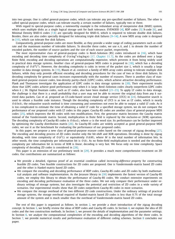
Fig. 2 shows an illustrative example for RDP codes. There are four data disks, D0, D1, D2 and D3, and each data disk consists of four data bits. Take D0 for instance, the four data bits are d0,0, d1,0, d2,0 and d3,0, which constitute a word. There are two parity disks. Each parity disk contains the same number of bits as a data disk. The first one is the row parity disk, denoted as P . Each parity bit is just the XOR of all the data bits in the corresponding row (see the upper part of Fig. 2). The other one is the diagonal parity disk, denoted as Q . The calculation of its parity bits involves not only the data packets, but also the bits in the row parity disk, P . As shown in the lower part of Fig. 2, the bits in the four data disks and the row parity disk, P , are classified into five diagonal sets. Each bit in the diagonal parity disk is the XOR of all the other elements in the same diagonal set. Take the parity bits q0 as an example, it is the XOR of all the elements in the first diagonal set, which contains d0,0, d3,2, d2,3 and p1. In this example, the word size, ω, is equal to 4, since four data bits are grouped together to form a single unit for encoding and decoding, as can be seen from Fig. 2 that a word of four bits is shown for each disk. For RDP codes, the word size, ω, has to satisfy two conditions: (i) ω ≥ k and (ii) ω + 1 is a prime number. RDP codes have excellent performance when ω = k, but the performance degrades as (ω − k) increases [3].

194 X. Gong, C.W. Sung / Journal of Computer and System Sciences 89 (2017) 190–208

4. Zigzag decodable codes

ZD Codes are designed as a class of general-purpose codes. The encoding and decoding process of ZD codes involve only bit-shift and XOR operations. They have two desirable properties, namely, k-reliability and zigzag decodability. Zigzag decodability means that the original file can be recovered by zigzag decoding. Before formally defining zigzag decoding, we first describe a mathematical representation of ZD codes. Given a source file s, we split it into k packets s1, s2, . . . , sk . Each packet si consists of L bits, and is represented by the following polynomial,

si(z) = si,0 + si,1z + si,2z2 + · · · + si,L−1zL−1, (2)

where si, j is an element of GF(2). The k source packets are linearly combined to obtain n coded packets c1(z), c2(z), . . . ,cn(z), each of which has L + l bits, where l denotes the maximum offset. The coded packet ci(z) is given by

ci(z) = zai,1 s1(z) + zai,2 s2(z) + · · · + zai,k sk(z), (3)

where i ∈ [1, n], and ti, j ∈ Z. Note that l = maxi, j ai, j . In theory, the coded packets can be of different lengths. For ease of analysis and presentation, we simply assume that dummy bits are appended to coded packets, so that they are of equal length. If systematic codes are used, we assume that the source packets are of length L while parity packets are of length L + l. For practical implementation, it is also more convenient to have equal-length parity packets.

The encoding procedure in (3) can be represented by the following matrix form,

c(z) = A(z)s(z), (4)

where c(z) is an n-dimensional vector whose i-th element is ci(z), s(z) is an k-dimensional vector whose j-th element is s j(z), and A(z) is an n × k matrix whose (i, j)-th element is zai, j . Our aim is to design a systematic erasure code. Define m � n − k, which represents the number of parity packets. The encoding matrix A(z) should be in the form of

A(z) =[

Ik×kB(z)

], (5)

where Ik×k is the k × k identity matrix and B(z) is an m × k matrix whose (i, j)-th element is αi, j(z) = zbi, j .Now it remains to design the matrix B(z). First of all, the code should be k-reliable, which implies that packets encoded

by any square submatrix M(z) of B(z) can be used to recover the source packets. Suppose the size of the given square matrix M(z) = [zti, j ] is k ×k, and we define M � {1,2, . . . ,k}. Besides, we introduce a k ×k integer matrix T = [ti, j], whose element is the exponent of the corresponding element in M(z). If the recovering process can be done by Algorithm 1, we say that the code is zigzag decodable. Note that the input to Algorithm 1 are k coded parity packets and the matrix T , while the output are the k source packets. The basic idea is to search for a coded packet that has an “exposed” bit, which can be directly read out. After that, the bit is subtracted from other coded packets. The procedure repeats until all source bits are decoded. An example to illustrate the execution of Algorithm 1 can be found in the Appendix.

Remark 1. In Algorithm 1, steps 18 and 19 are needed when all the L bits of source packet i have been decoded. In that case, the corresponding element, B[i][ j∗], is updated to a value that is large enough so that it will never be chosen in Step 12.

Remark 2. The computational complexity of Algorithm 1 is O (k2 L) due to the two for-loops in lines 10 and 15, respectively.

Remark 3. For practical implementation, the algorithm can be further sped up, as the sequence of coded packets that have “exposed” bits is eventually periodic (see the example in the Appendix). This feature has been incorporated into our software used in Section 5.

Now we are going to prove a sufficient condition on M(z) for zigzag decodability. For i ∈M, define

Si � arg minj∈M

ti, j. (6)

Note that Si is a set of integers. We say that Su � Sv if the smallest element in Su is greater than or equal to the largest element in Sv .

Definition 2 (Increasing difference property). A square matrix M(z) = [zti, j ] and its corresponding exponent T = [ti, j] are both said to satisfy the increasing difference property if given any i < i′ and j < j′ , we have

ti, j′ − ti, j < ti′, j′ − ti′ j.

X. Gong, C.W. Sung / Journal of Computer and System Sciences 89 (2017) 190–208 195

Algorithm 1 ZigZag decoding algorithm.Require: k binary arrays, Y1, Y2, . . . , Yk , each of length L + l, and a k × k integer array, TEnsure: k binary arrays, X1, X2, . . . , Xk , each of length L

// Initialization1: B := T ;2: Let V be the array of size L + l whose first L elements are equal to 1 and the last l elements are equal to 0;3: for i = 1 to k do4: pi := 1;5: for j = 1 to k do6: Let V j be obtained by cyclically shifting V to the right by T [i][ j] positions;7: end for8: Ai := V 1 + V 2 + · · · + Vk ;9: end for

10: for number of decoded bits = 1 to kL do11: Find the smallest i∗ such that Ai∗ [pi∗ ] = 1;12: j∗ := arg min j B[i∗][ j];13: b := Yi∗ [pi∗ ] and h := pi∗ − T [i∗][ j∗];14: X j∗ [h] := b;15: for i = 1 to k do16: pi := h + T [i][ j∗] and Yi [pi ] := Yi [pi ] ⊕ b;17: B[i][ j∗] := B[i][ j∗] + 1;18: if B[i][ j∗] − T [i][ j∗] − L = 0 then19: B[i][ j∗] := L + l + 1;20: end if21: if Ai [pi ] > 1 then22: Ai [pi ] := Ai [pi ] − 1;23: else24: pi := pi + 1;25: end if26: end for27: end for

This condition means that the relative offset between source packet j′ and j are increasing from parity packet i to i′ . Graphically, the source packets in parity packet i are “sliding” to the right to obtain parity packet i′ , as can be seen from the example in the Appendix (c4, c5, c6 and c7 in Fig. 13). This condition ensures that there is always a parity packet that has an “exposed” bit so that zigzag decoding can proceed. A proof now follows.

Lemma 1. Given any k × k matrix T that has the increasing difference property, S1, S2, . . . , Sk as defined in (6) satisfy the following properties:

(i) Si � Si′ if i ≤ i′ .(ii) |Si ∩ Si+1| ≤ 1, for i = 1, 2, . . . , k − 1.

(iii) ∪i∈MSi can be partitioned into the following k disjoint subsets: S1 \ S2, S2 \ S3, . . . , Sk−1 \ Sk, Sk.

Proof. (i) The first property is equivalent to this: If j ∈ Si and j′ ∈ Si′ , where i < i′ , then j ≥ j′ . We prove by contradiction by first assuming j′ < j. Then we have

ti, j′ − ti, j < ti′, j′ − ti′, j ≤ 0,

where the first inequality follows from the increasing difference property and the second one follows from the fact that j′ ∈ Si′ . As a consequence, we have

ti, j > ti, j′ ,

which contradicts with the fact that j ∈ Si .(ii) clearly follows from (i).(iii) We prove by mathematical induction. It is clear that S1 ∪ S2 can be partitioned into S1 \ S2 and S2. Assume that ⋃u

i=1 Si can be partitioned into

S1 \ S2,S2 \ S3, . . . ,Su−1 \ Su,Su,

for u ≥ 2. Consider ⋃u+1

i=1 Si . It can be partitioned into

S1 \ (S2 ∪ Su+1),S2 \ (S3 ∪ Su+1), . . . ,Su−1 \ (Su ∪ Su+1),Su+1.

Since (i) and (ii) together imply that for i = 1, 2, · · · , u − 1,

Si \ (Si+1 ∪ Su+1) = Si \ Si+1,

the statement is proved. �

196 X. Gong, C.W. Sung / Journal of Computer and System Sciences 89 (2017) 190–208

Theorem 2. Given k coded packets Y1, Y2, . . . , Yk and the encoding matrix M(z), which has the increasing difference property, zigzag decoding as stated in Algorithm 1 is able to recover source packets X1, X2, . . . , Xk.

Proof. Zigzag decoding can successfully recover the source packets if it can always find an interference-free symbol of a source packet from one of the encoded packet, or more formally, if it can always find i∗ in Step 11 of Algorithm 1 during each iteration. We prove by contradiction.

Recall that in Algorithm 1, B is initialized to T , which has the increasing difference property. After every iteration, B will be updated by adding an all-one vector to one of its columns. It is clear that such an operation keeps the increasing difference property unchanged. In other words, B always satisfies the increasing difference property.

Suppose the algorithm fails in Step 11 during a certain iteration. Based on the current value of B , we define Si for all i ∈M as in (6). Since the algorithm halts abnormally, we must have |Si | ≥ 2 for all i, for otherwise |Si | = 1 for some i and an “exposed” bit can be found. By Lemma 1(iii), we have

∣∣∣∣∣⋃

i∈MSi

∣∣∣∣∣ =k−1∑i=1

|Si \ Si+1| + |Sk|.

Since |Si| ≥ 2 for all i, by Lemma 1(ii), we have∣∣∣∣∣⋃

i∈MSi

∣∣∣∣∣ ≥ (k − 1) + 2 = k + 1 > k,

which is a contradiction. Therefore, the algorithm can always find i∗ in Step 11, which implies that we can always find an exposed bit and decode it out. The algorithm stops only when all bits of all source packets are determined. �

The following two constructions of ZD codes are designed based on this essential condition. The first one is inspired by Vandermonde matrix. We name the it as Vandermonde-matrix based ZD codes. The second one is derived from an Hankel matrix, so we call it Hankel-matrix based ZD codes.

4.1. Vandermonde-matrix based ZD codes

We now demonstrate a construction of ZD codes based on Vandermonde matrix. As stated before, our goal is to design an encoding matrix as in (5). In other words, we need to design the structure of B(z). Since the core idea of designing B(z) is to assign the offset of each source packet, which is represented by the exponent of each element in B(z). For convenience, we introduce an integer matrix P , whose element is the exponent of the corresponding element in B(z). Therefore, designing a code construction B(z) is equivalent to designing P .

In our construction, the m × k matrix B(z) takes the following form:⎡⎢⎢⎢⎣

1 1 · · · 11 z · · · zk−1

1...

. . ....

1 zm−1 · · · z(m−1)×(k−1)

⎤⎥⎥⎥⎦ , (7)

and the corresponding integer matrix P is given by⎡⎢⎢⎢⎣

0 0 · · · 00 1 · · · k − 1

0...

. . ....

0 m − 1 · · · (m − 1) × (k − 1)

⎤⎥⎥⎥⎦ . (8)

It is easy to check that any square submatrix of B(z) satisfies the increasing difference property. As a result, the code is zigzag decodable.

Note that the attractive low decoding complexity of ZD codes needs to sacrifice slight storage efficiency. For this code, the longest parity packet contains lV = (m − 1)(k − 1) more bits than the source packets. There are totally m parity packets, the proportion of extra storage overhead is at most m(m−1)×(k−1)

(k+m)L .

4.2. Hankel-matrix based ZD codes

Next, we consider another construction of ZD codes based on Hankel matrix, which has a smaller storage overhead. We will define the code structure by means of the integer matrix P , which is derived from the class of Hankel matrix.

X. Gong, C.W. Sung / Journal of Computer and System Sciences 89 (2017) 190–208 197

Definition 3. An N × N matrix H is called a Hankel matrix if it is in the following form,

⎡⎢⎢⎢⎢⎢⎣

h0 h1 h2 · · · hN−1h1 h2 h3 · · · hN

h2 h3 h4 · · · hN+1...

......

. . ....

hN−1 hN hN+1 · · · h2(N−1)

⎤⎥⎥⎥⎥⎥⎦

. (9)

For i, j ∈ {1, 2, . . . , N}, the (i, j)-th element of H , hi, j , satisfies

hi, j = hi+ j−2 (10)

for some given sequence h0, h1, . . . , h2(N−1) .

Given the value of N , in our code design, the values of h0, h1, · · · , h2(N−1) are specified as follows:

hN−1 = 0, (11)

and for i = 0, 1, 2, . . . , 2N − 3,

hi+1 − hi = i − N + 2. (12)

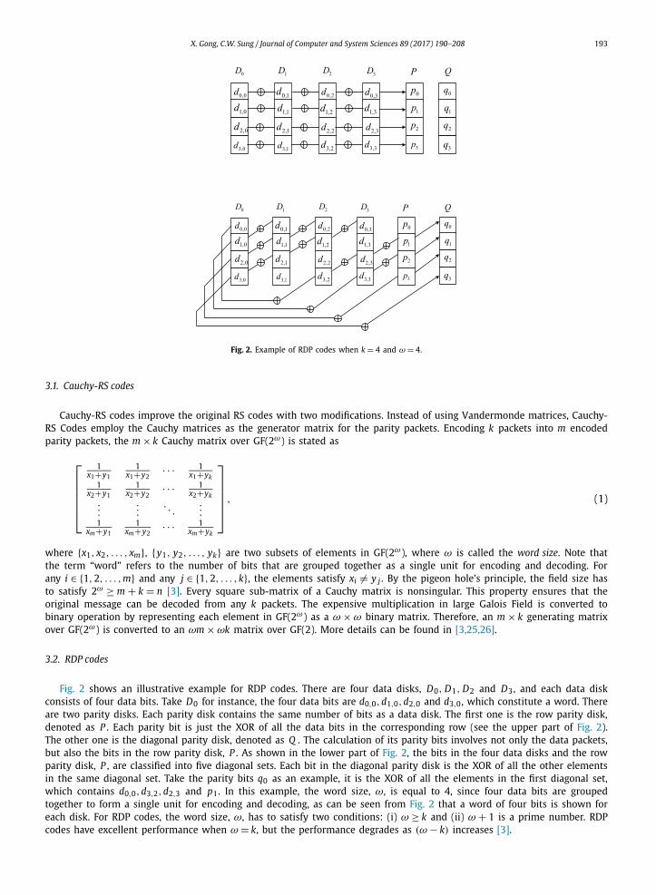
For example, when N = 4, we have h0 = 3, h1 = 1, h2 = 0, h3 = 0, h4 = 1, h5 = 3 and h6 = 6. According to (11) and (12), the Hankel matrix H 4×4 is given by

⎡⎢⎢⎣

3 1 0 01 0 0 10 0 1 30 1 3 6

⎤⎥⎥⎦ . (13)

Note that according to (11), the anti-diagonal of the matrix is always equal to zero. By (12) with i = N − 2, the anti-superdiagonal is also equal to zero.

Our code is constructed by specifying the m × k matrix P , which is obtained from a submatrix of the N × N Hankel matrix constructed by (11) and (12), where N = max {m,k}. If m < k, P is the submatrix consisted of the m rows of Hstarting from the row of index �(k − m)/2 + 1. Otherwise, P is the submatrix consisted of the k columns of H starting from the column of index �(m − k)/2 + 1. For example, if k = 3 and m = 4, then P should be the submatrix consisted of three columns starting from the column with index �(m − k)/2 + 1 = 1. According to (13), P is given by

⎡⎢⎢⎣

3 1 01 0 00 0 10 1 3

⎤⎥⎥⎦ . (14)

This is actually the code we considered in Example 1.Now we are going to prove that the matrix H constructed satisfies the increasing difference property.

Theorem 3. Given a Hankel matrix constructed by (11) and (12), if i < i′ and j < j′ , then

hi, j′ − hi, j < hi′, j′ − hi′, j . (15)

Proof. Consider first the case when j′ − j = 1. By (10) and (12), we have

hi, j′ − hi, j = hi+ j−1 − hi+ j−2

= (i + j − 2) − N + 2

< (i′ + j − 2) − N + 2

= hi′+ j−1 − hi′+ j−2

= hi′, j′ − hi′, j .

Now consider the general case when j′ > j. The above result implies the following set of inequalities:

198 X. Gong, C.W. Sung / Journal of Computer and System Sciences 89 (2017) 190–208

Fig. 3. Illustration of the Handkel matrix for the case when m ≥ k.

hi, j+1 − hi, j < hi′, j+1 − hi′, j

hi, j+2 − hi, j+1 < hi′, j+2 − hi′, j+1

...

hi, j′ − hi, j′−1 < hi′, j′ − hi′, j′−1

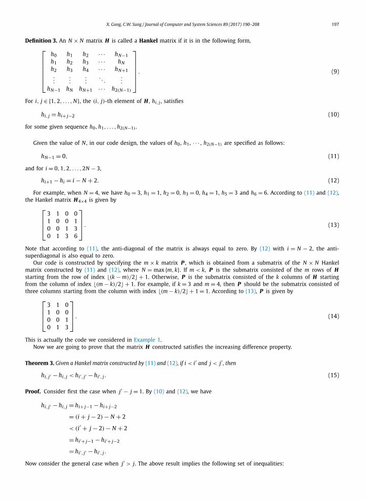
Summing them up, we obtain (15). �For Hankel-matrix based ZD codes, the maximum offset lH is the value of the bottom right element of matrix P , which

is equal to h j for some j between N − 1 and 2(N − 1). Due to the symmetry of H , it suffices to consider only the case when m ≥ k. Consider Fig. 3. Since the bottom left element of H is hN−1, the bottom left element of P is hi , where i = (N − 1) + �(m − k)/2 and the bottom right element of P is h j , where

j = i + k − 1

= (N − 1) +⌊

m + k

2

⌋− 1

= (N − 1) +⌊n

2

⌋− 1.

According to (11) and (12), the maximum offset is given by

lH = h j =j−1∑

i=N−1

(i − N + 2)

=�n/2 −1∑

k=1

k

= 1

2

(⌊n

2

⌋− 1

)⌊n

2

⌋

Consider the previous example when k = 3 and m = 4. It can be directly observed from (14) that the maximum offset, lH , is equal to 3, which agrees with the above expression.

Recall that the maximum offset of Vandermonde-matrix based ZD codes is

lV = (m − 1)(k − 1).

Depending on the values of the code parameters, it can be larger or smaller than lH . For example, if m is a fixed value, while n and k grow, then lV grows linearly with k while lH grows quadratically with n. Vandermonde-matrix based ZD codes clearly have a smaller storage overhead.

On the other hand, suppose we keep the proportion of parity packet keeps constant, i.e., k = αm for some fixed positive rational number α. In other words, the code rate R is a constant equal to α/(α + 1). Then, we have

lH ≤ 1

2

(n

2− 1

) n

2

= n(n − 2)

8

= (1 + α)2m2

8− (1 + α)m

4

X. Gong, C.W. Sung / Journal of Computer and System Sciences 89 (2017) 190–208 199

The maximum offset of the Vandermonde-matrix based ZD codes is

lV = αm2 − (1 + α)m + 1.

The difference of the maximum offsets of the two codes is

lV − lH = −1

8m2[(α − 3)2 − 8] + O (m). (16)

Hankel-matrix based ZD codes perform better if α satisfies 3 − 2√

2 ≤ α ≤ 3 + 2√

2, or 0.17 ≤ α ≤ 5.83. This corresponds to the case when the code rate satisfies 0.15 ≤ R ≤ 0.85. For practical applications, α, or equivalently, R , typically lies within the above range, so Hankel-matrix based ZD codes should have a lower storage overhead. Numerical comparisons of the extra storage overhead of these two codes for some common parameters for storage systems will be presented in Section 7.

5. Experiment settings

In this section, we describe the experiment settings, including the process of encoding and decoding, and settings of involved parameters. The input of the encoding experiment is a large source file with size around 1 GB. The output is a set of files with smaller size. To avoid confusion, we call these small files as subfiles, including k source subfiles and m parity subfiles. The k source subfiles are obtained by splitting the large source file into k pieces. The parity subfiles are calculated by different coding schemes. The input of the decoding experiment is a set of k subfiles selected from the (k + m) subfiles, i.e., the number of lost subfiles is set as m. Although the number of erasures can be less than or equal to m, and the erasures can happen to not only source subfiles, but also parity subfiles, losing m source subfiles is the most complex case in the decoding process of every coding scheme. And recovering the source file in high speed with most tolerable erasures is an important property in erasure code design. Thus we test the decoding speed of all coding schemes based on the case when m source subfiles are lost. Based on modern erasure-coded systems, such as Google File System [44,45], Facebook Hadoop Distributed File System [46] and Windows Azure Storage [47], and the analysis and discussion in [48–50], commonly used erasure codes have storage amounts of 1.33× to 2× of the original data file. Note that the storage amount of the traditional three-replication code is 3× of the data file size and the purpose of using other erasure codes is to reduce this 3× storage amount. We choose the combinations of (k, m) that are likely used in actual storage systems for our experiments. (6, 2) is the combination appeared in RAID-6 system. (6, 3) is chosen by Google II [44,45]. (10, 4) is the preference for HDFS-RAID in Facebook [46]. (12, 4) is considered to achieve good performance in Windows Azure Storage [47]. We also investigate the trend of encoding and decoding speeds as increasing number of source subfiles with four fixed ratios of storage overhead, which are 1.33×, 1.6×, 1.8×, and 2.0×. For every coding technique, each of these ratios has two corresponding curves describing its encoding and decoding speeds respectively. We choose four pairs of (k, m) for each curve. All the values of (k, m) taken for our experiments are stated in Table 2.

In many applications, the source file to be stored is often much larger than the memory size of most computers. In our experiments, we set the source file size as 1 GB. To encode such a large file, using a buffer to complete the process in a batch-wise fashion is a common solution. First, the data of source file are written into the buffer sequentially, until the buffer is full. The data in the buffer are then encoded. After encoding, the source data and parity data are written to the corresponding subfiles. The process is repeated until the whole file is encoded. Based on the results in [3], we set the buffer size to be the ballpark of 600 KB, which is sufficiently large to achieve efficient I/O. The parameters of source file size and buffer size are summarized in Table 2.

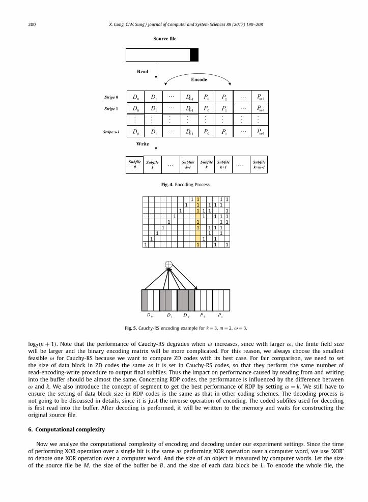
Now we illustrate the encoding of the data in the buffer. The buffer is partitioned into several contiguous memory space of equal size. Each of them is called a stripe. As shown in Fig. 4, the buffer consists of s stripes. In each stripe, there are k data blocks, D0, D1, . . . , Dk−1 and m parity blocks, P0, P1, . . . , Pm−1. The data in the m parity blocks are calculated from the data temporarily stored in the k source blocks based on a specific coding method. Apparently a stripe is a minimum collection of bits that encode and decode together. After encoding has finished, the data in the buffer will be written into the corresponding subfiles.

The reason for introducing the concept of stripe is that performing XOR operations over a group of bits is much faster than over a single bit. Also, load balancing can be easily realized with stripes. The size of one stripe depends on the size of each block. If we denote the size of source blocks as L bytes and the size of parity blocks as L′ bytes, then the stripe has a size of (kL + mL′) bytes. For ordinary coding schemes, L equals L′ , while it is not the case in our ZD codes. Since in ZD codes, we allow a little overhead in parity blocks, we have L′ > L. Once the block size is set, the number of stripes is only determined by the buffer size. In our experiment, L is set to be 4 KB and L′ is calculated according to the code construction of ZD codes. The chosen data block size is also stated in Table 2. In our implementation, the data in one stripe is allocated in consecutive address space to obtain good data locality. Data locality is the space difference of a sequence of memory access performed by a processor. Once a memory location is accessed, the processor will load a chunk of data in memory around the accessed location into the cache. Therefore, good data locality reduces cache miss and results in better performance.

The remaining problem is how to determine the parameter ω for RDP codes and Cauchy-RS codes. According to [3], we partition each data block into ω segments for Cauchy-RS codes. Thus the data block size equals to ω times the size of segment, P . Fig. 5 provides an example for encoding the first parity segment. According to [30], ω must be larger than

200 X. Gong, C.W. Sung / Journal of Computer and System Sciences 89 (2017) 190–208

Fig. 4. Encoding Process.

Fig. 5. Cauchy-RS encoding example for k = 3, m = 2, ω = 3.

log2(n + 1). Note that the performance of Cauchy-RS degrades when ω increases, since with larger ω, the finite field size will be larger and the binary encoding matrix will be more complicated. For this reason, we always choose the smallest feasible ω for Cauchy-RS because we want to compare ZD codes with its best case. For fair comparison, we need to set the size of data block in ZD codes the same as it is set in Cauchy-RS codes, so that they perform the same number of read-encoding-write procedure to output final subfiles. Thus the impact on performance caused by reading from and writing into the buffer should be almost the same. Concerning RDP codes, the performance is influenced by the difference between ω and k. We also introduce the concept of segment to get the best performance of RDP by setting ω = k. We still have to ensure the setting of data block size in RDP codes is the same as that in other coding schemes. The decoding process is not going to be discussed in details, since it is just the inverse operation of encoding. The coded subfiles used for decoding is first read into the buffer. After decoding is performed, it will be written to the memory and waits for constructing the original source file.

6. Computational complexity

Now we analyze the computational complexity of encoding and decoding under our experiment settings. Since the time of performing XOR operation over a single bit is the same as performing XOR operation over a computer word, we use ‘XOR’ to denote one XOR operation over a computer word. And the size of an object is measured by computer words. Let the size of the source file be M , the size of the buffer be B , and the size of each data block be L. To encode the whole file, the

X. Gong, C.W. Sung / Journal of Computer and System Sciences 89 (2017) 190–208 201

Table 1Encoding and decoding complexities of different erasure codes.

Encoding Decoding Operations

RDP 2M(k − 1)/k 2M(k − 1)/k XORCauchy-RS O (ωmM) O (ωMm) XOR

O (m2) Multiplication

ZD mM(k − 1)/k O (kM + m2 Mk ) XOR

same encoding or decoding process in one stripe has to repeat Ms/B = M/(kL) times. We do not count the shift operation, since the encoding and decoding algorithms only need to address the relevant word for XOR operation. Take the encoding of (2, 2) Vandermonde-matrix based ZD code as an example. To generate the i-th word of the second parity block for i ≥ 1, we can simply perform XOR between the i-th word of the first source block with the (i + 1)-th word of the second source block. It is not necessary to actually perform the shift operation.

For the encoding process of RDP codes, each row parity word requires at most k −1 XORs. There are ω rows in our array. ω(k − 1) XORs are required for row parity. Each diagonal parity word contains k data words or row parity words. Thus at most k − 1 XORs needed. There are ω diagonal parity words in an array, so ω(k − 1) XORs are required for diagonal parity. The number of such arrays in each stripe is equal to the size of segment. The number of XORs performed in one stripe is 2Pω(k − 1). Therefore, encoding a file of size M using RDP codes requires 2M(k − 1)/k XORs in total, which achieves the minimum number of XORs among all MDS array codes [5]. For decoding complexity, reconstructing any two data blocks is actually 2ω words. Each parity set is of size k words, so the cost to reconstruct each word is at most k − 1 XORs. The complexity for reconstructing the data blocks in one stripe is 2Pω(k − 1). With respect to the whole file, the complexity is again 2M(k − 1)/k XORs.

According to [25], the encoding complexity of Cauchy-RS for each parity block is O (kPω2) XORs. Therefore, O (ωMm)

XORs are required for encoding. Cauchy-RS requires O (kPmω2) XORs and O (m2) multiplications in GF(2ω) in each stripe for decoding process. Thus reconstruction of the original file requires O (ωMm) XORs and O (m2) multiplications in GF(2ω).

For ZD codes, (k − 1)mL XORs are required for encoding in each stripe. Since there are M/kL stripes, the whole encoding process needs mM(k −1)/k XORs. If k > m, during decoding, O ((k −m)mL) XORs are required to subtract the systematic part from the parity blocks in each stripe. Since (k − m)m ≤ k2

4 , the substraction step requires O (k2 L). Then zigzag decoding is used to decode the m parity blocks, which requires O (m2L) XORs (see Remark 2 of Algorithm 1). The operation in one stripe should be repeated M/(kL) times to finish decoding. The whole decoding process involves O (kM + m2 M

k ) XORs. If k < m, all systematic subfiles are lost. Performing the Zigzag decoding algorithm requires O (k2 L) XORs (again see Remark 2 of Algorithm 1). Thus we need O (kM) XORs for overall decoding. In conclusion, the total XORs required for overall decoding is at most O (kM + m2 M

k ). Note that for m proportional to k, both encoding and decoding complexities are linear. For the case of double failure, i.e., m = 2, the encoding complexity of ZD codes becomes O (M), which is the same as that of RDP codes. This agrees with our numerical results to be presented in the next section.

We summarize the encoding and decoding complexities of the three codes in Table 1. Recall that RDP applies only to the case when m = 2, so we first compare the performance of the three codes under this condition. For Cauchy-RS, the word size, ω, has to satisfy 2ω ≥ n. When m = 2 and k can be arbitrarily large, RDP and ZD have the same order of encoding complexity, which is lower than that of Cauchy-RS. Besides, RDP has the lowest decoding complexity. In other words, RDP has the best performance, which is expected as it is a special-purpose codes, which can only be used when m = 2.

Next, we consider the general case. We compare the performance between Cauchy-RS and ZD. It can be seen that ZD has lower encoding complexity than Cauchy-RS. For decoding, Cauchy-RS requires XOR and multiplication over GF(2ω), while ZD requires XOR only. The time complexity of multiplication depends on the implementation. For multiplication over finite field of characteristic 2, the most straightforward way is to simply perform bit-shift and bit-wise addition, which has time complexity of O (ω2). If the Karatsuba–Ofman Algorithm [51,52] is used, then it can be improved to O (ωlog2 3). As a result, the multiplication can be done in O (m2ωlog2 3) XORs. If M is fixed, then the decoding complexity of ZD codes is lower than that of Cauchy-RS. On the other hand, if M is large, then the time consumption of multiplication can be ignored. In this case, if m is fixed while k increases, then Cauchy-RS requires fewer XORs than ZD. If the relative storage overhead, m/k, is fixed and we let both m and k goes to infinity, then the decoding complexity of ZD is linear and is lower than that of Cauchy-RS by a factor of ω = log n.

7. Experiment results

While the computational complexity is obtained in the previous section, it is still necessary to obtain precise numerical results to evaluate their encoding and decoding speeds. Therefore, we implement ZD codes and RDP codes in C to test their encoding and decoding performance. For Cauchy-RS codes, Jeasure library in [30] is regarded as the best implementation. So we just use this library to realize Cauchy-RS codes in our experiment. According to the description in Section 4, we summarize the parameter settings in Table 2.

202 X. Gong, C.W. Sung / Journal of Computer and System Sciences 89 (2017) 190–208

Table 2Parameters setting.

(k,m) commonly used in today’s systems (6,2), (6,3), (10,4), (12,4)

(k,m) − 1.33× (12,4), (15,5), (18,6), (24,8)

(k,m) − 1.6× (12,7), (15,9), (18,10), (24,14)

Source file size 1 GBBuffer size 600 KBData block size 4 KB

Fig. 6. Performance of RDP codes, ZD codes and Cauchy-RS codes for k = 6, m = 2.

7.1. Encoding and decoding performance comparison

In this subsection we provide the numerical results based on our experiments. All the implementation programs are complied using gcc. Our test platform is a PC with Intel Core i5-2410 CPU running at 2.30 GHz with 8 GB of RAM, and a L1 cache of 32 KB and a L2 cache of 256 KB. We measure the time using the gettimeofday(), which is considered to be the most accurate timing function under Linux operating system. All of our results are the average of 10 runs. In Fig. 6, we show the performance of the encoding and decoding of the three different codes using box plot for the case where k = 6and m = 2. According to the figure, 10 runs is enough to obtain accurate estimate, as the variance of the ten samples is very small for each of the three codes. For better visual effect, we plot our experimental results using bar chart in other figures.

When it comes to the double-parity case, according to the results shown in Fig. 6, the encoding performance of ZD codes are nearly the same as that of RDP codes, and both RDP and ZD codes outperform Cauchy-RS by roughly 20%. The RDP encoding process requires almost 1.734 GB of XORs, which is actually the same as the XORs required for ZD encoding. This result agrees with the computational complexity analysis in section 5. The encoding time of RDP is even slightly larger than that of ZD codes. This is reasonable because the XOR computing in RDP codes has poorer data address continuity than ZD codes, which may lead to more time for addressing and more cache misses. On the other hand, the decoding performance of ZD codes is not as good as the other two codes. The reason is that we decode one computer word per iteration during the decoding process of ZD codes, which implies large space difference between subsequent memory access. It leads to a lot of cache misses and results in poor performance. That is also the reason for worse decoding performance of ZD codes than that of Cauchy-RS codes when (k, m) = (6, 3), as can be seen from Fig. 8. However, compared with Cauchy-RS codes in the case of (k, m) = (6, 3), the encoding time of ZD codes has been reduced by 24.74%. Also, as shown in Fig. 7 and 8, ZD codes have better performance than Cauchy-RS codes in terms of both encoding and decoding when (k, m) = (10, 4) and (k, m) = (12, 4). We also investigate the number of XORs performed by ZD codes and Cauchy-RS codes. According to Fig. 9, the number of XORs during the encoding process of ZD codes is 20% less than that of Cauchy-RS codes when (k, m) = (6, 2). And the advantage increases to 39.6% when (k, m) = (12, 4). With respect to decoding, as shown in Fig. 10 the number of XORs performed by Cauchy-RS codes is 10.42% more than that performed by ZD codes when (k, m) = (6, 2). In the case of (k, m) = (12, 4), Cauchy-RS codes require 62.04% more XORs required by ZD codes.

X. Gong, C.W. Sung / Journal of Computer and System Sciences 89 (2017) 190–208 203

Fig. 7. Encoding performance of ZD codes and Cauchy-RS codes for (k,m) ∈ {(6,3), (10,4), (12,4)}.

Fig. 8. Decoding performance of ZD codes and Cauchy-RS codes for (k,m) ∈ {(6,3), (10,4), (12,4)}.

Fig. 9. Number of XORs performed during encoding process of ZD and Cauchy-RS for (k,m) ∈ {(6,2), (6,3), (10,4), (12,4)}.

Fig. 11 and 12 provide the encoding time and decoding time of the two codes for two different levels of storage overhead, which are 1.33× and 1.6×. As the number of source subfiles increases, the encoding and decoding times of both ZD codes and Cauchy-RS codes are increasing with the growth of k. However, the encoding and decoding times of Cauchy-RS increase much more quickly than those of ZD codes. As the word size ω of Cauchy-RS should increase with the growth of k + m. Larger value of ω implies more complicated binary encoding matrix for Cauchy-RS and more operations in finite field. Therefore, larger value of ω results in worse performance of Cauchy-RS, which is consistent with the result in [3]. And our results show that ZD codes outperforms Cauchy-RS codes at least 45.77% in encoding time and at least 19.70% in decoding time when ω = 5. When ω = 6, encoding time is reduced by at least 59.67% and decoding time is reduced by at least 46.93%.

204 X. Gong, C.W. Sung / Journal of Computer and System Sciences 89 (2017) 190–208

Fig. 10. Number of XORs performed during decoding process of ZD and Cauchy-RS for (k,m) ∈ {(6,2), (6,3), (10,4), (12,4)}.

Fig. 11. Encoding performance of ZD and Cauchy-RS for 1.33× and 1.6×.

Fig. 12. Decoding Performance of ZD and Cauchy-RS for 1.3× and 1.6×.

X. Gong, C.W. Sung / Journal of Computer and System Sciences 89 (2017) 190–208 205

Table 3Overhead calculations.

(k,m) (6,2) (6,3) (10,4) (12,4)

Vandermonde-based ZD 0.0305% 0.0813% 0.1883% 0.2014%Hankel-based ZD 0.0366% 0.0488% 0.1465% 0.1709%

7.2. Storage overhead of ZD codes

As we mentioned, ZD codes introduce a little extra storage overhead to obtain high encoding and decoding performance. The actual value of overhead depends not only on specific code construction, but also the implementation settings. We summarize the proportion of storage overhead based on our analysis and experiment settings in Table 3. Suppose L′ is the size of parity block, and L is the size of data block. The overhead is normalized over total storage amount needed for ordinary MDS codes as m(L′−L)

(k+m)L .As shown in the table, the price to pay for ZD codes is negligible, and better performance in encoding and decoding can

be obtained in return.

8. Conclusion

A new class of erasure codes, called ZD codes, is designed. Two constructions, which are based respectively on the Vandermonde matrix and the Hankel matrix, are presented. They belong to the class of ZD codes because both of them satisfy the increasing difference property, which is proved to be a sufficient condition for zigzag decodability. The most attractive feature of the ZD codes is that both the encoding and decoding algorithms can be performed in linear time and involve only XOR and bit-shift operations. Such a linear time complexity is lower than those of all existing general-purpose erasure codes that has the combination property. The only price to pay is that the size of parity packets is slightly larger than those of classical MDS codes. This extra overhead, however, is negligible for data storage applications, in which the packet size is typically very large.

To evaluate its practical applicability, we implement the encoding and decoding of the code in C programming language. Based on our implementation, we compare the encoding and decoding performance of ZD codes with RDP codes and Cauchy-RS codes. Since RDP is specially designed for RAID-6, which supports only double parity, it performs better than the other two codes, which are general-purpose codes, as expected. To compare ZD codes with Cauchy-RS codes, a detailed experimental study has been carried out. When the number of total packets n, including source packets and parity packets, is less than 16, encoding and decoding of ZD codes is faster than Cauchy-RS codes under the often used parameter settings of practical storage systems. It performs worse than Cauchy-RS codes only when the coding parameters are very small. When n is larger than 16, the encoding performance of ZD codes is far better than Cauchy-RS codes, and the decoding performance of ZD codes is at least 20% better than that of Cauchy-RS codes.

In addition to actual computation time of encoding and decoding, we have also measured the number of XOR operations required by the two codes. Experimental results show that ZD codes always require fewer XOR operations in both encoding and decoding, even if the coding parameters are very small. This result hints that cache miss is the key factor which adversely affects the decoding time of ZD codes. While the actual encoding and decoding times of ZD codes are greater than Cauchy-RS codes for small parameters such as (k, m) = (6, 3), this result depends heavily on today’s computer architecture. The required numbers of XOR operations of the two codes, however, are machine-independent. If the codes are compared not on general-purpose computers, but on specially designed hardware platforms, ZD codes have the potential to outperform Cauchy-RS even for very small coding parameters.

Acknowledgment

This work was partially supported by a grant from the University Grants Committee of the Hong Kong Special Adminis-trative Region, China (Project No. AoE/E-02/08).

Appendix A. Example of zigzag decoding algorithm

Now we illustrate the idea of ZD codes and the associated decoding method as stated in Algorithm 1 by walking through the following example:

Example 1. Let n = 7, k = 3, m = 4, and

B(z) =

⎡⎢⎢⎣

z3 z 1z 1 11 1 z1 z z3

⎤⎥⎥⎦ .

206 X. Gong, C.W. Sung / Journal of Computer and System Sciences 89 (2017) 190–208

Fig. 13. Coded packets when n = 7, k = 3, m = 4.

Fig. 14. Example of Zigzag Decoding when n = 7, k = 3, m = 4.

The seven coded packets are graphically shown in Fig. 13. Now we explain how zigzag decoding algorithm works, assuming that the three parity packets, c5, c6, and c7, are used for decoding.

The three input parity packets for decoding, y1, y2 and y3 are shown in Fig. 14. The k ×k input integer array, T , is given by

T =⎡⎣ 1 0 0

0 0 10 1 3

⎤⎦ , (A.1)

X. Gong, C.W. Sung / Journal of Computer and System Sciences 89 (2017) 190–208 207

whose (i, j)-th entry, where 1 ≤ i, j ≤ 3, represents the amount of bit-offset of source packet j in the i-th packet for decoding.

The first step of the algorithm is to initialize the variable matrix B as T . Note that the i-th row of this variable matrix records the offset of the first not-yet-decoded bit of the source packets in the i-th coded packet for decoding. Then from Step 2 to Step 9, we compute k integer arrays Ai for each yi , where Ai[ j] indicates how many source packets are XORed together to obtain the j-th bit of yi . The initial value of Ai is given under each coded packet in Fig. 14. Besides, the variable pi in Step 4 represents the first not-yet-decoded bit in the i-th coded packet for decoding. All the p′

i s are initialized to 1.

The decoding procedure is carried out in the for-loop starting from Step 10. In Step 11, the lowest-indexed coded packet with an exposed bit is identified. Consider the first iteration, the smallest i∗ such that Ai∗ [pi∗ ] = 1 is 3, implying A3 has an exposed bit while A1 and A2 do not. Now we have to find which source packets contribute to this exposed bit. It is performed by finding the smallest element in the i∗-th row of B and returning the position. In this case, the smallest element is B[3][ j∗], where j∗ = 1. Therefore, s j∗ = s1 is the source packet that contributes to this exposed bit. Note that the offset of source packet s1 in encoding y3 is T [3][1] = 0. Thus it must be the bit of position h := pi∗ − T [3][1] = 1 in s1that was enrolled in the exposed bit, and the value of the exposed bit is b := Y3[p∗

3] = Y3[1], as shown in Step 13. Now we may conclude X1[h] = X1[1] := b, as shown in Step 14. X1[1] in fact is equal to the first bit of s1, i.e., s1,0.

Before entering into the next iteration, we need to update some variables, which are done in Steps 15∼26. The bit decoded out should be subtracted from the three encoded packets. It is executed by the following XOR operations in Step 16:

Y1[2] := Y1[2] ⊕ b,

Y2[1] := Y2[1] ⊕ b,

Y3[1] := Y3[1] ⊕ b.

The matrix B , which records the offset of the first not-yet-decoded bit of source packets, is updated by adding 1 to each element in its j∗-th column, i.e., the first column in our example:

B := B +⎡⎣ 1 0 0

1 0 01 0 0

⎤⎦ =

⎡⎣ 2 0 0

1 0 11 1 3

⎤⎦ .

Also the k binary arrays which indicate the number of overlapping source packets should be updated as follows:

A1 := [2 2 3 · · · 3 2 1 0 0

] ;A2 := [

1 2 3 · · · 3 3 1 0 0] ;

A3 := [0 2 2 · · · 3 3 2 1 1

].

The value of p3 becomes 2, meaning that next time we start from A3[2] to find the smallest i∗ in Step 11. In other words, pi always points to the first non-zero element of Ai .

In this example, it is easy to see that the sequence of coded packets that have “exposed” bits is 3, 2, 1, 3, 2, 1, ..., which is periodic. This feature can be exploited to further speed up the decoding algorithm.

References

[1] M.K.M. Shahabinejad, M. Ardakani, An efficient binary locally repairable code for hadoop distributed file system, IEEE Commun. Lett. 18 (8) (2014) 1287–1290.

[2] M.S. Hwang, C.H. Lee, Secure access scheme in mobile database systems, Eur. Trans. Telecommun. 12 (4) (2001) 303–310.[3] J.S. Plank, J. Luo, C.D. Schuman, L. Xu, Z. Wilcox-O’Hearn, A performance evaluation and examination of open-source erasure coding libraries for storage,

in: Proceedings of FAST, USENIX Association, Berkeley, CA, USA, 2009, pp. 253–265.[4] M. Blaum, J. Brady, J. Bruck, J. Menon, Evenodd: an efficient scheme for tolerating double disk failures in raid architectures, IEEE Trans. Comput. 44 (2)

(1995) 192–202.[5] P. Corbett, B. English, A. Goel, T. Grcanac, S. Kleiman, J. Leong, S. Sankar, Row-diagonal parity for double disk failure correction, in: Proceedings of the

3rd USENIX Symposium on File and Storage Technologies (FAST ’04, 2004, pp. 1–14.[6] L. Xu, J. Bruck, X-code: MDS array codes with optimal encoding, IEEE Trans. Inf. Theory 45 (1) (1999) 272–276, http://dx.doi.org/10.1109/18.746809.[7] M. Blaum, R.M. Roth, On lowest-density MDS codes, IEEE Trans. Inf. Theory 45 (1999) 46–59.[8] J.S. Plank, The RAID-6 liberation codes, in: Proceedings of the 6th USENIX Conference on File and Storage Technologies, USENIX Association, Berkeley,

CA, USA, 2008, pp. 7:1–7:14.[9] J.B.J.M.M. Blaum, J. Brady, A. Vardy, The EVENODD code and its generalization, in: High Performance Mass Storage and Parallel I/O, 2001, pp. 187–208.

[10] G. Feng, R. Deng, F. Bao, J. Shen, New efficient MDS array codes for RAID, Part I: Reed–Solomon-like codes for tolerating three disk failures, IEEE Trans. Comput. 54 (9) (2005) 1071–1080.

[11] M. Blaum, A family of MDS array codes with minimal number of encoding operations, in: IEEE International Symposium on Information Theory, 2006, pp. 2784–2788.

[12] C. Huang, L. Xu, STAR: an efficient coding scheme for correcting triple storage node failures, IEEE Trans. Comput. 57 (7) (2008) 889–901.[13] G.L.Y. Wang, X. Zhong, Triple-star: a coding scheme with optimal encoding complexity for tolerating triple disk failures in RAID, Int. J. Innov. Comput.

Inf. Control 3 (2012) 1731–1742.[14] I. Tamo, Z. Wang, J. Bruck, Zigzag codes: MDS array codes with optimal rebuilding, IEEE Trans. Inf. Theory 59 (2013) 1597–1616.

208 X. Gong, C.W. Sung / Journal of Computer and System Sciences 89 (2017) 190–208

[15] M.H.H. Hou, K.W. Shum, New MDS array code correcting multiple disk failures, in: Global Communications Conference (GLOBECOM), IEEE, 2014, pp. 2369–2374.

[16] I. Reed, G. Solomon, Polynomial codes over certain finite fields, J. Soc. Ind. Appl. Math. 8 (2) (1960) 300–304.[17] R.E. Blahut, Theory and Practice of Error Control Codes, Addison Wesley, Reading, MA, 1984.[18] G. Feng, R. Deng, F. Bao, J. Shen, New efficient MDS array codes for RAID, Part II: Rabin-like codes for tolerating multiple (≥ 4) disk failures, IEEE Trans.

Comput. 54 (9) (2005) 1473–1483.[19] M. Blaum, J. Bruck, A. Vardy, MDS array codes with independent parity symbols, IEEE Trans. Inf. Theory 42 (2) (1996) 529–542, http://dx.doi.org/

10.1109/18.485722.[20] J.S. Plank, M.G. Thomason, A practical analysis of low-density parity-check erasure codes for wide-area storage applications, in: DSN-2004: The Inter-

national Conference on Dependable Systems and Networks, IEEE, 2004, pp. 115–124.[21] J.W. Byers, M. Luby, M. Mitzenmacher, A. Rege, A digital fountain approach to reliable distribution of bulk data, ACM SIGCOMM Comput. Commun. Rev.

28 (4) (1998) 56–67.[22] M. Luby, LT codes, in: Proc. of the 43rd Aunnual IEEE Symposium on Foundations of Computer Science (FOCS’02), Washington, DC, USA, 2002,

pp. 271–282.[23] A. Shokrollahi, Raptor codes, IEEE Trans. Inf. Theory 52 (6) (2006) 2551–2567.[24] N. Cao, S. Yu, Z. Yang, W. Lou, Y. Hou, LT codes-based secure and reliable cloud storage service, in: 2012 Proceedings IEEE INFOCOM, 2012, pp. 693–701.[25] J. Blomer, M. Kalfane, R. Karp, M. Karpinski, M. Luby, D. Zuckerman, An XOR-Based Erasure-Resilient Coding Scheme, Tech. rep., 1995.[26] J.S. Plank, L. Xu, Optimizing Cauchy Reed–Solomon codes for fault-tolerant network storage applications, in: Fifth IEEE International Symposium on

Network Computing and Applications, NCA 2006, 2006, pp. 173–180.[27] S. Gollakota, D. Katabi, Zigzag decoding: combating hidden terminals in wireless networks, in: V. Bahl, D. Wetherall, S. Savage, I. Stoica (Eds.), SIGCOMM,

ACM, 2008, pp. 159–170.[28] X. Fu, Z. Xiao, S. Yang, Overhead-free in-place recovery scheme for XOR-based storage codes, in: Proceedings of IEEE Int. Conf. Trust, Security and

Privacy in Computing and Commun., Beijing, China, Sep. 2014, pp. 552–557.[29] C.W. Sung, X. Gong, A zigzag-decodable code with the MDS property for distributed storage systems, in: Proceedings of IEEE ISIT, Istanbul, Turkey, Jul.

2013, pp. 341–345.[30] J.S. Plank, S. Simmerman, C.D. Schuman, Jerasure: A Library in C/C++ Facilitating Erasure Coding for Storage Applications, Tech. rep., 2007.[31] J. Qureshi, C.H. Foh, J. Cai, Optimal solution for the index coding problem using network coding over GF(2), in: 2012 9th Annual IEEE Communications

Society Conference on Sensor, Mesh and Ad Hoc Communications and Networks (SECON), 2012, pp. 209–217.[32] A. Al-Shaikhi, J. Ilow, Design of packet-based block codes with shift operators, EURASIP J. Wirel. Commun. Netw. 2010 (2010) 263210, http://dx.

doi.org/10.1155/2010/263210.[33] H. Hou, K.W. Shum, M. Chen, H. Li, BASIC regenerating code: binary addition and shift for exact repair, in: Proceedings of IEEE ISIT, Istanbul, Turkey,

Jul. 2013, pp. 1621–1625.[34] C.W. Sung, X. Gong, Combination network coding: alphabet size and zigzag decoding, in: 2014 International Symposium on Information Theory and

Its Applications (ISITA), Melbourne, Australia, 2014, pp. 699–703.[35] T. Nozaki, Fountain codes based on zigzag decodable coding, in: 2014 International Symposium on Information Theory and its Applications (ISITA),

Melbourne, Australia, 2014, pp. 274–278.[36] M. Li, P.P.C. Lee, STAIR codes: a general family of erasure codes for tolerating device and sector failures in practical storage systems, in: Proceedings of

the 12th USENIX Conference on File and Storage Technologies (FAST ’14), Santa Calra, CA, Feb. 2014.[37] Z. Wang, A.G. Dimakis, J. Bruck, Rebuilding for array codes in distributed storage systems, in: Proc. IEEE Globecom Workshops, Miami, USA, 2010,

pp. 1905–1909.[38] Y. Zhu, P.P.C. Lee, L. Xiang, Y. Xu, L. Gao, A cost-based heterogeneous recovery scheme for distributed storage systems with RAID-6 codes, in: Pro-

ceedings of the 2012 42Nd Annual IEEE/IFIP International Conference on Dependable Systems and Networks (DSN), DSN ’12, IEEE Computer Society, Washington, DC, USA, 2012, pp. 1–12.

[39] Y. Zhu, P. Lee, Y. Xu, Y. Hu, L. Xiang, On the speedup of recovery in large-scale erasure-coded storage systems, IEEE Trans. Parallel Distrib. Syst. 25 (7) (2014) 1830–1840, http://dx.doi.org/10.1109/TPDS.2013.244.

[40] H. Hou, K.W. Shum, M. Chen, H. Li, BASIC codes: low-complexity regenerating codes for distributed storage systems, IEEE Trans. Inf. Theory 62 (6) (2016) 3053–3069.

[41] S. El Rouayheb, K. Ramchandran, Fractional repetition codes for repair in distributed storage systems, in: 2010 48th Annual Allerton Conference on Communication, Control, and Computing (Allerton), 2010, pp. 1510–1517.

[42] Q. Yu, C.W. Sung, T.H. Chan, Irregular fractional repetition code optimization for heterogeneous cloud storage, IEEE J. Sel. Areas Commun. 32 (5) (2014) 1048–1060.

[43] C. Huang, L. Xu STAR, An efficient coding scheme for correcting triple storage node failures, IEEE Trans. Comput. 57 (7) (2008) 889–901.[44] A. Fikes, Storage architecture and challenges, 2010.[45] D. Ford, F. Labelle, F. Popovici, M. Stokely, V.-A. Truong, L. Barroso, C. Grimes, S. Quinlan, Availability in globally distributed storage systems, in:

Proceedings of the 9th USENIX Symposium on Operating Systems Design and Implementation, 2010.[46] D. Borthakur, HDFS RAID, Nov. 2010.[47] C. Huang, H. Simitci, Y. Xu, A. Ogus, B. Calder, P. Gopalan, J. Li, S. Yekhanin, Erasure coding in Windows Azure Storage, in: Presented as Part of the

2012 USENIX Annual Technical Conference (USENIX ATC 12), USENIX, Boston, MA, 2012, pp. 15–26.[48] S. Narayanamurthy, Modern erasure codes for distributed storage systems, Storage Developer Conference, SNIA, Bangalore, http://www.snia.org/sites/

default/files/SDC/2016/presentations/erasure_coding/Srinivasan_Modern_Erasure_Codes.pdf.[49] M. Xia, M. Saxena, M. Blaum, D.A. Pease, A tale of two erasure codes in HDFS, in: 13th USENIX Conference on File and Storage Technologies (FAST 15),

USENIX Association, Santa Clara, CA, 2015, pp. 213–226.[50] D. EMC, Ecs 2.0 – understanding data protection, https://www.emc.com/techpubs/ecs/ecs_data_protection-1.htm#GUID-2847BF53-4247-4124-9668-

11FCBABF015C.[51] A. Karatsuba, Y. Ofman, Multiplication of multidigit numbers on automata, Sov. Phys. Dokl. 7 (7) (1963) 595–596.[52] A. Weimerskirch, C. Paar, Generalizations of the Karatsuba algorithm for efficient implementations, https://eprint.iacr.org/2006/224.pdf.