Contents lists available at ScienceDirect

Journal of Development Economics

journal homepage: www.elsevier.com/locate/jdeveco

Population density, fertility, and demographic convergence in developingcountries

David de la Croixa,b,⁎, Paula E. Gobbic,a

a IRES, Université catholique de Louvain, Place Montesquieu 3, B-1348 Louvain-la-Neuve, Belgiumb CORE, Université catholique de Louvain, Place Montesquieu 3, B-1348 Louvain-la-Neuve, Belgiumc National Fund for Scientific Research, Belgium

A R T I C L E I N F O

JEL classification:J13D19O18R11

Keywords:Demographic and Health SurveyFertilityPreventive checkAgglomeration externalitiesPopulation dynamics

A B S T R A C T

Whether the population tends towards a long-run stationary value depends on forces of demographicconvergence. One such force is the result of fertility rates being negatively affected by population density. Wetest the existence of such an effect in 44 developing countries, matching georeferenced data from theDemographic and Health Surveys for half a million women with population density grids. We find a causalrelationship from population density to fertility such that a rise in density from 10 to 1000 inhabitants persquare kilometer corresponds to a decrease in fertility of about 0.7 children. The corresponding half-life forpopulation dynamics is of the order of four–five generations.

1. Introduction

Long-run population projections are key to assessing the sustain-ability of our societies. The combination of current age structures andprojected fertility levels produces relatively accurate projections with ahorizon of 50 years, but longer-term predictions rapidly becomeuncertain (Livi-Bacci, 1997). In the projections made by thePopulation Division of the UN, fertility being estimated in terms ofeither a high or low scenario (United Nations, 2004; Gerland et al.,2014) determines the time and level at which global population willpeak. The probabilistic projections of the UN (Gerland et al., 2014) orof IAASA (Lutz and Butz, 2014) would benefit from a reduction in theuncertainty surrounding fertility.1 In general, the speed at which Africaexperiences the demographic transition matters to determine the peakof the world population. Consequently, gaining a better understandingof the determinants of fertility is a priority in order to improve theselong-run forecasts.

We study whether or not fertility behavior reflects spontaneousconvergence forces that lead the population to a stable, long-run level.In the natural sciences, this property is called population homeostasis(Lee, 1987). In animal populations, predator–prey models may display

such a property, depending on their parameters. In human popula-tions, predators are absent, but human reproduction is subject tolimited resources. If convergence forces are at work, one shouldobserve a correlation between fertility and/or mortality and populationdensity. At high levels of density, fertility should be low, and/ormortality high, for a population to stabilize. The contribution of thispaper is to shed light on the existence of the channel relating fertility topopulation density in developing countries.2

There are different ways in which population density may affectfertility. For Malthus (1807), areas with higher population density havelower agricultural income, and marriage and fertility are delayed(preventive check) as compared to regions with lower densities.According to a more modern view, initiated by Sadler et al. (1830),while income is higher in more densely populated areas because ofagglomeration externalities, fertility decreases with income, leading tothe same final negative relationship between density and fertility. Moredensely populated areas may also yield decreased fertility because theyoffer more affordable or accessible education and health infrastructure.

Beyond these causal mechanisms, the sorting (selection) of indivi-duals can generate an apparent correlation between density andfertility. This is the case when people who are less inclined to have

http://dx.doi.org/10.1016/j.jdeveco.2017.02.003Received 22 January 2016; Received in revised form 14 February 2017; Accepted 14 February 2017

⁎ Corresponding author at: IRES, Université catholique de Louvain, Place Montesquieu 3, B-1348 Louvain-la-Neuve, Belgium.E-mail addresses: david.delacroix@uclouvain.be (D. de la Croix), paula.gobbi@uclouvain.be (P.E. Gobbi).

1 The difference between these two recent projections essentially stems from different assumptions about Chinese and Nigerian fertility rates.2 Mortality can also be affected by population density. For example, André and Platteau (1998) detail the path from population pressure to land conflicts, and, ultimately to violence

and genocide in Rwanda.

Journal of Development Economics 127 (2017) 13–24

Available online 17 February 20170304-3878/ © 2017 Elsevier B.V. All rights reserved.

MARK

children migrate to more densely populated places to enjoy the greaterincome opportunities offered by cities (Courgeau, 1989) and/or thosewho are more inclined to have children move to regions where thepopulation density is lower and where raising children costs less. Inthis case, population density may not have a causal relationship tofertility, but instead may only affect individual decisions with respect towhere to live. The United Nations (2014) projects that 66% of theworld's population will live in urban areas by 2050. In 1950, this figurewas only 30%. This movement of people from rural to urban areas maybe the result of a selection of individuals and may not reflect an effect ofhigher population density on individual decision-making.

To analyze the relationship between population density and ferti-lity, we use different sources of data. Raster files for population densitycome from CIESIN et al. (2011). They are based on detailed populationdata from census administrative units.3 Individual fertility data arefrom the Demographic and Health Surveys (DHS) for 44 developingcountries. In the DHS data, individuals belong to clusters, which aregeoreferenced, allowing for mapping population density onto fertility.In order to control for geographic variables, the caloric suitability indexdeveloped by Galor and Özak (2014) is used to control for intrinsic landquality. We also use the CIESIN et al. (2011) data to control for thedistance to large bodies of water. Satellite light data are used to controlfor income effects at a disaggregated level.

We first consider the cluster level (i.e. village or neighborhood),relating the average number of births in a given cluster to thepopulation density of this cluster. Without any control apart fromcountry fixed effects, geographic variables, and the mean age of womenin the cluster, an increase in population density from 10 to 1000inhabitants decreases fertility by about one child on average. Whencontrolling for additional cluster characteristics such as education,mortality, and income, the size effect is divided by four but remainshighly significant. Among all the controls, education seems particularlyimportant, indicating that education is obtained more easily in denselypopulated areas, where traveling costs are lower, and the fixed costs ofschools are more easily covered (Boucekkine et al., 2007).

This relationship could be biased due to an omitted variableproblem. Places with greater unobserved amenities might be those towhich individuals with certain traits moved in the past and where thesetraits have persisted. This could lead to a spurious relationship in whichit is not population density that affects fertility rates, but rather theunobserved characteristics of the people living in areas with a specificpopulation density. We therefore use the distance to buildings and citiesbelonging to UNESCO World Heritage Sites constructed between theNeolithic Revolution and 1900, as a proxy for past population density,to instrument current population density. Controlling for currentincome, the exclusion restriction is that this instrument has no effecton fertility, other than through population density. We argue that thisinstrument reflects incentives for people to move to these specific areaslong ago. However, the main reason why people are still in these areastoday is the persistence of population density. Using this instrument, weestimate an even larger effect of population density on fertility, showingthat endogeneity biases have a tendency to attenuate its effect.

In order to further exclude the possibility that population density atthe cluster level may proxy local spillovers that affect fertility, weanalyze fertility behavior at the individual level, distinguishing betweenindividual and cluster effects (e.g. for education). The results aresimilar to those at the cluster level. The individual-level analysis alsoallows us to study whether or not the relationship between populationdensity and fertility is the result of selection. Controlling for migrationdoes not alter the conclusion; estimates from a subsample of indivi-duals who had not moved during their lifetime are very similar to thosefrom the whole sample.

Other papers have documented a negative relationship betweenpopulation density and fertility, but never at the individual level.Among others, Adelman (1963) and Heer (1966) showed such apattern for country-level data. By today's standards, however, it wouldbe hard to argue that the correlation they found does not reflectcountry-specific factors (e.g. institutions) that were not accounted forin their analyses. A more robust approach would be to use countrypanel data, as in Lutz and Qiang (2002) and Lutz et al. (2006), whoemphasize the importance of including population density as adeterminant of declining fertility rates. Another approach is to comparesmaller entities within the same country. For example, Firebaugh(1982) shows that population density and fertility were negativelyrelated across 22 Indian villages between 1961 and 1972. However,these approaches limit the analysis to aggregate level data. Thisincreases the likelihood of endogeneity due to the presence ofunobserved factors affecting both the fertility of a population and itsdensity. Compared to this literature, this paper is based on a muchbroader set of data (490k women in 25k clusters from 44 developingcountries). The analysis is also carried out at the individual level andprovides support for a causal effect of density on fertility.

The paper is organized as follows: the data are presented in Section2. Our cluster and individual analysis is provided in Sections 3 and 4respectively. The interpretation of the results for population dynamicsis provided in Section 5. The conclusions are presented in Section 6.

2. Data

We use a large data set including individual and householdsurveys carried out in 44 developing countries and estimate therelationship between fertility and other variables, among populationdensity.

To relate population density to fertility, information from demo-graphic surveys must be combined with geographical data on popula-tion density and other controls, such as the quality of the land or thedistance to water. Individual and household characteristics are derivedfrom Demographic and Health Surveys (DHS), which in most countriesare geo-localized. We have incorporated all countries with “StandardDHS” type data sets available, selecting the waves that are closest to theyear 2000. Households are grouped into clusters for which we have thelatitude and the longitude from the DHS GPS file.4 The raster files forworld population density are taken from CIESIN et al. (2011), whichprovides information on population density in grids with a cell size of30″ × 30″ (approximately 1 km2).5 To avoid a possible reverse causalityfrom fertility to population density, we use density in 1990, which isthe earliest year available. Corrections for other types of endogeneitywill be implemented in the next two sections. Fig. 1 shows the positionof all the DHS clusters in our sample and their respective populationdensity. Unlike most of the recent literature using geographical data,our unit of analysis is not a cell but a point. The sample contains 24,769points.

To control for the geographical determinants of land productivity,we use one of the caloric suitability indexes developed by Galor andÖzak (2014) which has a resolution of 5′ × 5′ (approximately 10 km2).Galor and Özak (2015) show that the caloric suitability index dom-inates the conventionally used agricultural suitability data(Ramankutty et al., 2002) in terms of capturing the effect of landproductivity. In this paper, we use the raster file for the maximumpotential caloric yield attainable given the set of all suitable crops in thepost-1500 period. This yield varies across cells depending on theirclimatic and geographic characteristics, such as elevation, temperature,

3 See URL http://sedac.ciesin.columbia.edu/downloads/docs/gpw-v3/balk_etal_geostatpaper_2010pdf-1.pdf for methodological details.

4 DHS are built to be representative of a country's population. However, even if theyare not representative, it would not affect our study, since we do not consider country-level total fertility rates.

5 A map of the population density of the relevant region is provided in Fig. B.1,Appendix B.

D. de la Croix, P.E. Gobbi Journal of Development Economics 127 (2017) 13–24

14

rainfall, soil quality, terrain ruggedness, steepness, etc. Fig. B.2represents this variable.

Finally, as a proxy for income per capita, we use the GDP measuresfrom Ghosh et al. (2010), which are essentially based on night-timelight satellite data. Henderson et al. (2012) show that luminosity is astrong proxy for GDP. Apart from the fact that there is no standardizedmethod to account for national income across countries, and thatinformal sectors, which are often important in developing countries,are difficult to include in national statistics, the major advantage ofusing this data is that it allows us to capture total economic activity at adisaggregated level. The precision level of the raster is 30″ × 30″;however, measurement errors at the pixel level are large.6 Ashrafet al. (2015) argue in favor of measuring GDP on the basis of acontinuum of a larger number of night-time light pixels. We thereforebase our measure on an aggregated 20′ × 20′ raster. To obtain a percapita variable, we divide GDP by our measure of population densitytaken at the same level of aggregation and discarding pixels with fewerthan 0.1 inhabitant per km2. For every cluster, we impute its GDP asthe mean within a 50 km-radius circle. The resulting measure is shownin Fig. B.3. As an alternative measure, we also directly take the satellitelight data averaged over 1992–2013, and compute a per capitameasure as above, after having removed the areas affected by gasflares (from NOAA's “Global Gas Flaring Estimates”).

Let us come back to the DHS data and provide more details on thedata itself. We use the individual recode, the household recode, and theGPS data set. The list of the DHS data sets, with the correspondingyears and phases, are shown in Table B.1, in Appendix B. The totalnumber of clusters and individuals included in the sample are alsoprovided at the end of the table.

Table 1 provides the list of variables used, and some descriptivestatistics. From the individual recode, we build a sample consisting ofwomen between 15 and 49 years of age whose cluster we know.7 Wedrop the observations for which the number of years of education isunknown or is higher than 30. All dates are expressed in CenturyMonth Code (CMC).8 Mortality rates are computed as the ratio between

the total number of living children and the total number of childrenever born. Marital status is coded as either ever married (includesliving with a partner, currently married, divorced, or widowed) orsingle (never married). Data on religion is available for almost allcountries, except the following six: Bolivia, Colombia, Egypt, Morocco,Pakistan, and Peru. For countries for which we do have this informa-tion, we divide the sample into Muslims, Christians, Hindus,Buddhists, and others.9 Except for Burundi, Comoros, Lesotho,Liberia, Madagascar, Rwanda, Swaziland, Tanzania, Zimbabwe,Egypt, Jordan, Morocco, Bolivia, Bangladesh, Cambodia, andIndonesia, we also know the ethnicity each woman belongs to (notreported in the table). Fig. B.6, in Appendix B, shows the histogram ofthe variables: age, education, infant mortality, and number of births.We observe strong age heaping at ages ending in 0 and 5, which isevidence of women's ignorance of their actual age. Finally, it is worthnoting that the quality of the data on the number of children ever bornand their date of birth is subject to misreporting errors, as stressed inthe literature on demography (Schoumaker, 2014). We address thisissue in Section 4.4.

From the household recode, we use the information on whether ornot the household has electricity or/and a refrigerator. These twovariables are used as additional controls to proxy for income.

From the GPS data set, we use the geographical coordinates of eachcluster. From these, we can infer population density, land productivity,and income per capita in each cluster. In order to ensure the anonymityof respondents, urban clusters contain a minimum of 0 and amaximum of 2 km of positional error. Rural clusters contain aminimum of 0 and a maximum of 5 km of error, with a further 1%of rural clusters displaced a maximum of 10 km.10 To account for thiserror in urban clusters, we set the density in a cluster to the averagedensity in the 2 km radius around the center of this cluster. For ruralclusters, we set the radius at 5 km.11 Finally, as the raster for the caloric

Fig. 1. Cluster localization and population density. Note: Population density is reported as ln(1 + population density).

6 For example, they can be due to over-glow and blooming. We also check whether oneshould correct for gas flares, but the measure from Ghosh et al. (2010) seems to havefiltered them out.

7 In a majority of DHS, eligible individuals include women of reproductive age (15–49). Some countries provide information for older women, but we did not keep theseobservations in the sample.

8 CMC is the usual way in which dates are coded in DHS. Time is counted in terms ofmonths and starts with the value 1 for January 1900.

9 Christians include those who belong to the Roman Catholic Church, the EvangelicalChurch, the Anglican Church, Protestants, Seventh Day Adventists, Pentecostalists,Methodists, the Salvation Army, Kimbanguists, the “Églises Réveillées”, Presbyterians,the Apostolic Sect, the “Iglesia Ni Kristo”, the Aglipay (Philippine Independent Church),and those coded as “other Christians” by DHS.

10 DHS do not precisely define the urban–rural variable of the GPS data set. In eachcountry, they adopt a definition that can depend on the size of the population or on thebreadth of infrastructures. See more at URL: http://dhsprogram.com/What-We-Do/GPS-Data-Collection.cfm.

11 Due to the DHS displacement, two clusters in Uganda appear to be inside LakeVictoria. We give each point the minimal radius so as to have positive population density:

D. de la Croix, P.E. Gobbi Journal of Development Economics 127 (2017) 13–24

15

suitability index described above has a lower resolution than thepopulation density raster, we impute the land productivity in eachcluster from the value of the index in its given position.

3. Cluster-level analysis

We proceed in three steps. First, we show the relationship betweenpopulation density and development across clusters. Then, we showestimates for the correlation between fertility and population densitywith ordinary least squares (OLS). Then we discuss possible endo-geneity issues, and support a causal relationship between populationdensity and fertility using an instrumental variable estimation. Thewhole section uses cluster-level analysis.

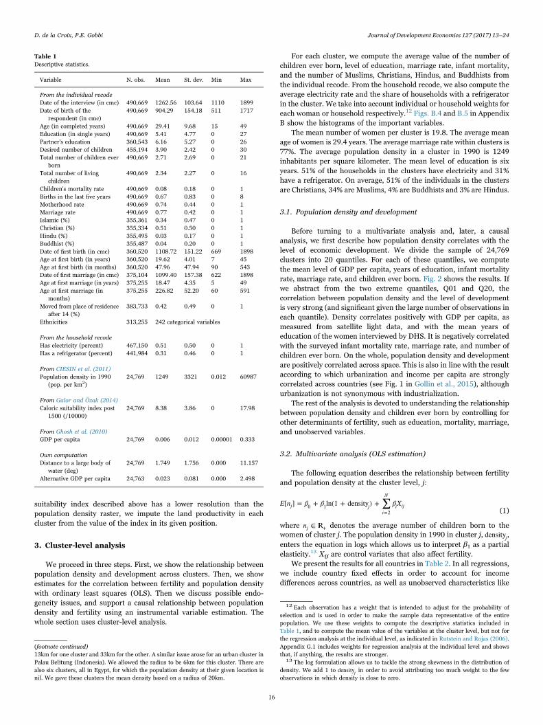
For each cluster, we compute the average value of the number ofchildren ever born, level of education, marriage rate, infant mortality,and the number of Muslims, Christians, Hindus, and Buddhists fromthe individual recode. From the household recode, we also compute theaverage electricity rate and the share of households with a refrigeratorin the cluster. We take into account individual or household weights foreach woman or household respectively.12 Figs. B.4 and B.5 in AppendixB show the histograms of the important variables.

The mean number of women per cluster is 19.8. The average meanage of women is 29.4 years. The average marriage rate within clusters is77%. The average population density in a cluster in 1990 is 1249inhabitants per square kilometer. The mean level of education is sixyears. 51% of the households in the clusters have electricity and 31%have a refrigerator. On average, 51% of the individuals in the clustersare Christians, 34% are Muslims, 4% are Buddhists and 3% are Hindus.

3.1. Population density and development

Before turning to a multivariate analysis and, later, a causalanalysis, we first describe how population density correlates with thelevel of economic development. We divide the sample of 24,769clusters into 20 quantiles. For each of these quantiles, we computethe mean level of GDP per capita, years of education, infant mortalityrate, marriage rate, and children ever born. Fig. 2 shows the results. Ifwe abstract from the two extreme quantiles, Q01 and Q20, thecorrelation between population density and the level of developmentis very strong (and significant given the large number of observations ineach quantile). Density correlates positively with GDP per capita, asmeasured from satellite light data, and with the mean years ofeducation of the women interviewed by DHS. It is negatively correlatedwith the surveyed infant mortality rate, marriage rate, and number ofchildren ever born. On the whole, population density and developmentare positively correlated across space. This is also in line with the resultaccording to which urbanization and income per capita are stronglycorrelated across countries (see Fig. 1 in Gollin et al., 2015), althoughurbanization is not synonymous with industrialization.

The rest of the analysis is devoted to understanding the relationshipbetween population density and children ever born by controlling forother determinants of fertility, such as education, mortality, marriage,and unobserved variables.

3.2. Multivariate analysis (OLS estimation)

The following equation describes the relationship between fertilityand population density at the cluster level, j:

∑E n β β βX[ ] = + ln(1 + density ) +j ji

N

i ij0 1=2 (1)

where n ∈j + denotes the average number of children born to thewomen of cluster j. The population density in 1990 in cluster j, densityj,enters the equation in logs which allows us to interpret β1 as a partialelasticity.13 Xij are control variates that also affect fertility.

We present the results for all countries in Table 2. In all regressions,we include country fixed effects in order to account for incomedifferences across countries, as well as unobserved characteristics like

Table 1Descriptive statistics.

Variable N. obs. Mean St. dev. Min Max

From the individual recodeDate of the interview (in cmc) 490,669 1262.56 103.64 1110 1899Date of birth of the

respondent (in cmc)490,669 904.29 154.18 511 1717

Age (in completed years) 490,669 29.41 9.68 15 49Education (in single years) 490,669 5.41 4.77 0 27Partner's education 360,543 6.16 5.27 0 26Desired number of children 455,194 3.90 2.42 0 30Total number of children ever

born490,669 2.71 2.69 0 21

Total number of livingchildren

490,669 2.34 2.27 0 16

Children's mortality rate 490,669 0.08 0.18 0 1Births in the last five years 490,669 0.67 0.83 0 8Motherhood rate 490,669 0.74 0.44 0 1Marriage rate 490,669 0.77 0.42 0 1Islamic (%) 355,361 0.34 0.47 0 1Christian (%) 355,334 0.51 0.50 0 1Hindu (%) 355,495 0.03 0.17 0 1Buddhist (%) 355,487 0.04 0.20 0 1Date of first birth (in cmc) 360,520 1108.72 151.22 669 1898Age at first birth (in years) 360,520 19.62 4.01 7 45Age at first birth (in months) 360,520 47.96 47.94 90 543Date of first marriage (in cmc) 375,104 1099.40 157.38 622 1898Age at first marriage (in years) 375,255 18.47 4.35 5 49Age at first marriage (in

months)375,255 226.82 52.20 60 591

Moved from place of residenceafter 14 (%)

383,733 0.42 0.49 0 1

Ethnicities 313,255 242 categorical variables

From the household recodeHas electricity (percent) 467,150 0.51 0.50 0 1Has a refrigerator (percent) 441,984 0.31 0.46 0 1

From CIESIN et al. (2011)Population density in 1990

(pop. per km2)24,769 1249 3321 0.012 60987

From Galor and Özak (2014)Caloric suitability index post

1500 (/10000)24,769 8.38 3.86 0 17.98

From Ghosh et al. (2010)GDP per capita 24,769 0.006 0.012 0.00001 0.333

Own computationDistance to a large body of

water (deg)24,769 1.749 1.756 0.000 11.157

Alternative GDP per capita 24,763 0.023 0.081 0.000 2.498

(footnote continued)13km for one cluster and 33km for the other. A similar issue arose for an urban cluster inPalau Belitung (Indonesia). We allowed the radius to be 6km for this cluster. There arealso six clusters, all in Egypt, for which the population density at their given location isnil. We gave these clusters the mean density based on a radius of 20km.

12 Each observation has a weight that is intended to adjust for the probability ofselection and is used in order to make the sample data representative of the entirepopulation. We use these weights to compute the descriptive statistics included inTable 1, and to compute the mean value of the variables at the cluster level, but not forthe regression analysis at the individual level, as indicated in Rutstein and Rojas (2006).Appendix G.1 includes weights for regression analysis at the individual level and showsthat, if anything, the results are stronger.

13 The log formulation allows us to tackle the strong skewness in the distribution ofdensity. We add 1 to densityj in order to avoid attributing too much weight to the fewobservations in which density is close to zero.

D. de la Croix, P.E. Gobbi Journal of Development Economics 127 (2017) 13–24

16

institutions. Standard errors are clustered at the country level.Column (1) of Table 2 shows the effect of population density on

fertility, controlling for nothing but the mean age in the cluster,geographical controls (land quality and distance to a large body ofwater), and country fixed effects. Controlling for land productivityaccounts for the Malthusian argument according to which moreproductive land leads to the fathering of more children by means ofan income effect. In other words, it allows us to control for the carryingcapacity of each location. The point estimates imply that if populationdensity increases from 10 ind/km2 to 1000 ind/km2, then the women in acluster would have 0.86 fewer children on average.14 To clarify thisfurther, Appendix D plots the maps of locations with densities ranging

from 0.01 to 10, 000 ind/km2.The introduction of marriage rates in Column (2) diminishes the

direct effect of population density. This may reflect the fact that peoplemarry later in more densely populated areas, which reduces theobserved marriage and birth rates in the cluster. In Column (3), weintroduce the infant mortality rate at the cluster level as a determinantof fertility. A higher mortality is purported to increase fertility as aresult of the child replacement effect (Doepke, 2005). The impact ofdensity on fertility is reduced by the inclusion of mortality (thereduction is statistically significant, but small in size). Infant mortalitycaptures part of the effect of density: as the provision of health servicesis higher in more densely populated areas, mortality is lower, decreas-ing the need to have a large number of children.

In Column (4), we also control for differences in GDP per capita

Fig. 2. Bivariate correlations at the cluster level between population density and: ln(GDP per capita) (top-left panel), years of education (top-right panel), infant mortality rates (middle-left panel), marriage rates (middle-right panel), and children ever born (bottom panel).

14−0.191 × (ln(1001) − ln(11)).

D. de la Croix, P.E. Gobbi Journal of Development Economics 127 (2017) 13–24

17

across clusters as wealthier places could for example have higherreturns to human capital and therefore a lower fertility, which would bein line with Beckerian theory (Doepke, 2015) . The impact of density onfertility is not altered significantly when controlling for the GDP percapita of the cluster, as shown in Column (4). Using the satellite lightdata over 1992–2003 as a proxy for GDP per capita does not lead to adifferent estimated correlation coefficient between fertility and popula-tion density. Finally, in Column (5) we add mothers’ level of educationas a control. The squared term is significant, showing a strongernegative effect of education on fertility for higher education levels. Asimilar argument to the one used to discuss mortality can be appliedhere. The provision of education services is higher in more denselypopulated areas, enabling mothers to become more educated. Moreeducation leads to lower fertility rates either because the opportunitycost of having children is higher, or because women are more aware ofcontraception. The estimate in Column (5) provides a lower bound onthe partial correlation between density and fertility, as all the maincontrols have been introduced. Under this specification, fertilitydecreases by 0.23 children when population density increases from10 ind/km2 to 1, 000 ind/km2.

Appendix E provides the results pertaining to the relationshipbetween population density and fertility for each continent. Themagnitudes of the relationships between fertility and populationdensity across different contexts remain remarkably similar to theestimates at the global level, shown in Table 2. The coefficients of ln (1+density) in Model (5) are −0.044 in Sub-Saharan Africa, −0.040 in theMiddle East and North Africa, −0.025 in Asia, and −0.052 in LatinAmerica (all significant at the 1% level, except for Asia, where thesignificance is at the 10% level). Finally, in order to account for the factthat some regions have transitioned to the modern growth regime,while others remain in the Malthusian stage, we also group countriesaccording to two income levels: countries belonging to the leastdeveloped economies according to the United Nations Economic andSocial Council (N = 25), and the remaining, wealthier, countries(N = 19). The results are presented in Appendix F. The effect of densityis significant in both samples, with a size of −0.030 for the poorestcountries, and −0.056 for the richest.

3.3. Causal inference (two-stage least squares)

One might suspect that the coefficient of density estimated by OLSis plagued by an endogeneity bias due to a local omitted variableaffecting both population density and women's fertility. This could leadto a spurious relationship between these two variables without causaleffect. Reverse causality is unlikely for two reasons: (i) we take theearliest available data for population density and the latest available forfertility rates. Therefore, fertility cannot affect past density and (ii)fertility is measured at the individual level while population density ismeasured at the cluster level.

Three candidates for omitted variables could affect both fertilityrates and population density. First, favorable economic conditionscan affect both fertility and population density, as people are morelikely to want to live in these places. We control for income in severalways. In the specification of Column 5 in Table 2, we control for GDPper capita using satellite night-light data, individuals’ education, andcountry fixed effects as proxies for income. Therefore, income isunlikely to affect fertility rates via a channel other than populationdensity.

A second omitted variable could be the existence of norms relatedto fertility. These could be linked to certain ethnicities rather thancountries, as we already control for country fixed effects. A regioninhabited by groups of individuals that observe a pro-natalist norm orexperience higher fecundity will have a higher population density as aresult. If our instrument cannot account for this persistence, then thebias introduced reduces the estimated impact of population density onfertility. This leads to a conservative estimate and therefore does notinvalidate the claim that population density has a causal impact onfertility. A similar argument can be made in the presence of unobservedfecundity factors specific to ethnicities.

Lastly, unobserved amenities at the local level can lead to themigration of people with certain characteristics whose persistencecould affect fertility rates.

If the omitted variables we have just described affect both popula-tion density and fertility positively, then they will attenuate themeasured effect of density on fertility in the regressions withoutinstrumentation. Instrumenting population density should thereforeincrease the effect of population density on fertility rates.

The generally accepted means of dealing with omitted variables is toinstrument the suspected endogenous variable. Density is a commonlyused variable in studies on firm productivity, as a way of capturingagglomeration effects. As surveyed by Combes and Gobillon (2015), theliterature has adopted different strategies to address this issue. Twostrategies dominate: using the historical value of population densityand using geographical and geological variables that were importantwith regard to human settlements centuries ago, but only havenegligible effects on outcomes today. The exogeneity of both types ofinstruments may depend on whether or not one is able to control forlocal permanent characteristics that may have affected past locationchoices and still affect fertility locally.

We instrument historical density with the distance to buildings andcities belonging to UNESCO World Heritage Sites constructed betweenthe Neolithic Revolution and 1900. Appendix C shows the list of thesesites and maps the computed distance to each cluster in our sample.Notice that we only retain man-made structures and not naturalhabitats. Proximity to a UNESCO World Heritage Site is likely toincrease population density on average since these sites were trade,religious, or political centers. While these were all good reasons toreside close to these locales at the time, they no longer apply since theyare not used for their original purpose anymore. However, if populationdensity is persistent over time, then this is a strong instrument. Thereare reasons to believe that some of these sites may still affect incometoday. For example, Valencia Caicedo (2014) shows that JesuitMissions on Guarani land have had a persistent effect on the educationand income of those who live close to them today. As we control for

Table 2OLS estimates at the cluster level.

Dependent variable:Children ever born, per woman (average in cluster)

(1) (2) (3) (4) (5)

ln(1+density) −0.191*** −0.142*** −0.125*** −0.119*** −0.050***(0.001) (0.007) (0.007) (0.007) (0.005)

Marriage 2.204*** 1.842*** 1.818*** 1.102***(0.101) (0.079) (0.081) (0.085)

Infant mortality 4.238*** 4.133*** 2.635***(0.484) (0.480) (0.314)

ln (GDP percapita)

−0.076*** −0.047***

(0.013) (0.011)Women's

education−0.091***

(0.024)(Women's

education)2−0.004**

(0.002)

Observations 24,769 24,769 24,769 24,769 24,769Adjusted R2 0.569 0.631 0.667 0.669 0.740

Notes: Robust standard errors, clustered at the country level, in parentheses. Allspecifications include country fixed effects, geographical controls (the caloric suitabilityindex and distance to a large body of water) and a polynomial of order 2 in mean age.* p < 0.1, ** p < 0.05, *** p < 0.01.

D. de la Croix, P.E. Gobbi Journal of Development Economics 127 (2017) 13–24

18

both the mean education and income of clusters, this should not lead usto violate the exclusion restriction.

A potential issue that could invalidate the instrument may be thatthe proximity to UNESCO World Heritage Sites affects fertility by wayof an institutional channel, namely the antiquity of the state. Thesemonuments could indeed symbolize great societies of the past whoseeffects persist today via norms. Indeed, Chanda and Putterman (2007)show that ancient states such as Egypt, China, and India still have anadvantage today, perhaps as a result of culture and institutionalcapabilities. Most of this effect is controlled for by the inclusion ofcountry fixed effects. Finally, one may still wonder whether someendogeneity bias may persist despite instrumentation through endur-ing norms. This type of bias would, however, play out in our favor.Indeed, since this persistence leads to a positive relationship betweenpopulation density and fertility rates, our estimate from the second-stage instrumental variable regression is a lower bound for the effect ofpopulation density on fertility. In all cases, the presence of countrydummies helps satisfy the exclusion restriction, as many historical andgeographical determinants of institutions possibly affecting fertility arecontrolled for.

Table 3 presents the results. Column (5) of Table 3 is the same asthat of Table 2. The second column shows the estimates for the firststage, and the third the estimates of the second stage. The F-test for thefirst stage is greater than the various threshold values proposed in theliterature. We therefore reject the hypothesis that the instrument isweak. We see that the effect of population density on fertility is, asexpected, stronger than in the benchmark of Column (5). The effect ofincreasing density from 10 to 1, 000 ind/km2 now leads to a drop of 0.64children, instead of 0.23 in the model without instrumentation. Theendogeneity bias is therefore an attenuation bias, arising from thepositive correlation between an unobserved variable and both densityand fertility.

4. Causal inference at the individual level

The analysis above reveals the main determinants of fertility ratesat the cluster level. Moving to the individual level allows us todisentangle the effects of personal variables, like one's education, fromthe effect of the environment, like the mean education in the cluster.

Kravdal (2013) argues that there are strong educational spillovers fromcluster-level data to individual behavior.

To exclude the fact that population density at the cluster level mayproxy such spillovers, thereby influencing individual fertility, in thissection we study fertility at the individual level. We also look at whetherthe selection of migrants with different fertility behaviors into more orless dense areas might have biased the results of the previous section.We then add further controls in order to account for individualdifferences in religion, ethnicity, and additional income levels.Finally, we discuss the quality of the fertility responses in DHS. Weconclude this section with a discussion of the identified mechanismsthat link population density to fertility rates.

4.1. Poisson and IV Poisson

Since the dependent variable, children ever born nj, is a countvariable, we estimate a Poisson regression model to predict the impactof density on births. The model is:

⎪

⎪

⎪

⎪

⎧⎨⎩

⎫⎬⎭∑E n π π π X[ ] = exp + ln(1 + density ) +j j

i

N

i ij0 1=2 (2)

where n ∈j is distributed according to a Poisson distribution. Theestimated coefficients π cannot be directly compared to the β's of theOLS. They are related through β π E n= [ ]i i j . Building on Eq. (1), in Eq.(2), we add controls for average education, marriage, and mortalityrates in the cluster where the woman lives. The results are shown inTable 4. To facilitate comparison with the regression at the clusterlevel, Column (x) of Table 4 has the same set of variates as Column (x)of Table 2. Column (5-IV) shows the estimates of an IV Poissonregression in which we instrument population density with the sameinstrumental variable used in Section 3.3, i.e. the distance to aUNESCO World Heritage Site, using the GMM estimation methoddescribed in Windmeijer and Santos Silva (1997).

The relationship between density and fertility estimated in Column(1) is close to that at the cluster level. Indeed,π E n× [ ] = − 0.069 × 2.711 = − 0.187j1 can be compared toβ = − 0.1911 . The estimate from Column (5) is not statistically differentfrom that at the cluster level either. As in the cluster analysis,instrumentation leads to a greater effect of density on the number ofchildren born; when population density goes from 10 to 1, 000 ind/km2,we estimate that fertility decreases by 0.7 children at the individuallevel. This again reflects the attenuation bias brought about by theomitted variables.

Among the additional control variables included at the individuallevel, it is worth noting the coefficient of education. At the cluster level,the effect of education on fertility is negative, with an increasingimpetus given by the quadratic term as the level of education increases.As stressed in Kravdal (2002), this measured effect combines bothindividual and aggregate effects. When one distinguishes between thetwo, the individual effect first increases and then decreases. Baudinet al. (2015) and Vogl (2016) find evidence of positive income effectsaffecting the fertility of the uneducated in a large number of developingcountries. This may explain the hump-shaped relationship betweeneducation and fertility found at the individual level. The other controlshave the same effect as at the cluster level, with the exception of thecluster-level marriage rate.15

The results shown in Table 4, and in all subsequent tables, do notaccount for individual weights. Appendix G.1 reproduces Table 4introducing individual weights. Table G.1 of this appendix shows that

Table 3IV estimates at the cluster level.

Dependent variable:nj ln(1+density) nj

(5) 1st stage 2nd stage

ln(1+density) −0.050*** −0.141***(0.005) (0.027)

Distance to UNESCO site −0.180***(0.023)

Marriage 1.102*** −1.744*** 0.941***(0.085) (0.304) (0.115)

Infant mortality 2.635*** −0.263 2.597***(0.314) (0.406) (0.307)

ln(GDP per capita) −0.047*** −0.263*** −0.019(0.011) (0.074) (0.013)

Women's education −0.094*** 0.341*** −0.063**(0.024) (0.050) (0.025)

Women's education2 −0.004** −0.001 −0.004**(0.002) (0.003) (0.002)

Observations 24,769 24,769 24,769Adjusted R2 0.740 0.469 0.722F-test 61.029***

Notes: Robust standard errors, clustered at the country level, in parentheses. Allspecifications include country fixed effects, geographical controls (the caloric suitabilityindex and distance to a large body of water) and age polynomials. * p < 0.1, ** p < 0.05,*** p < 0.01.

15 In the last two columns of Table 4, the coefficient of the average marriage rate in thecluster is negatively related to the fertility of individuals. This might be the result of thefollowing: in clusters where marriage rates are higher, the chance of finding a partner inthe event of divorce is lower and women may therefore choose to have fewer children inorder to limit the cost of divorcing.

D. de la Croix, P.E. Gobbi Journal of Development Economics 127 (2017) 13–24

19

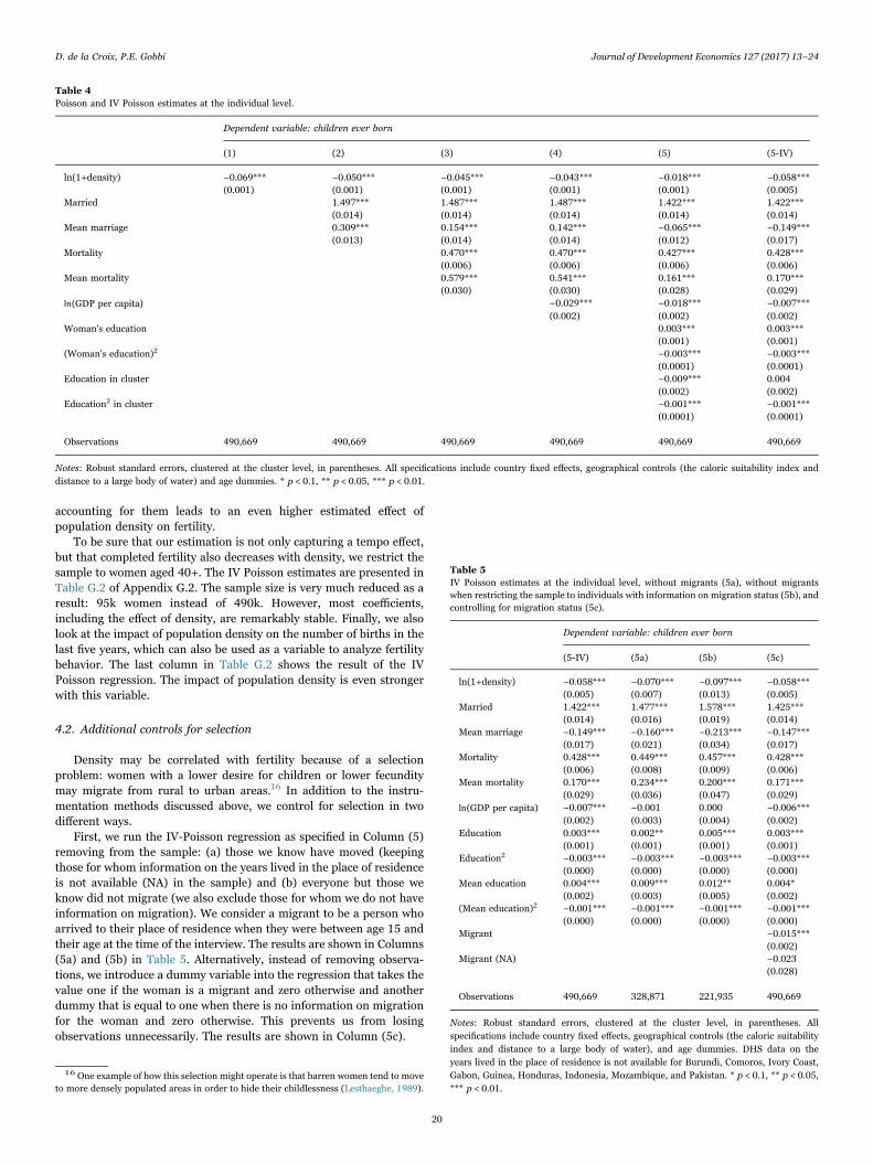
accounting for them leads to an even higher estimated effect ofpopulation density on fertility.

To be sure that our estimation is not only capturing a tempo effect,but that completed fertility also decreases with density, we restrict thesample to women aged 40+. The IV Poisson estimates are presented inTable G.2 of Appendix G.2. The sample size is very much reduced as aresult: 95k women instead of 490k. However, most coefficients,including the effect of density, are remarkably stable. Finally, we alsolook at the impact of population density on the number of births in thelast five years, which can also be used as a variable to analyze fertilitybehavior. The last column in Table G.2 shows the result of the IVPoisson regression. The impact of population density is even strongerwith this variable.

4.2. Additional controls for selection

Density may be correlated with fertility because of a selectionproblem: women with a lower desire for children or lower fecunditymay migrate from rural to urban areas.16 In addition to the instru-mentation methods discussed above, we control for selection in twodifferent ways.

First, we run the IV-Poisson regression as specified in Column (5)removing from the sample: (a) those we know have moved (keepingthose for whom information on the years lived in the place of residenceis not available (NA) in the sample) and (b) everyone but those weknow did not migrate (we also exclude those for whom we do not haveinformation on migration). We consider a migrant to be a person whoarrived to their place of residence when they were between age 15 andtheir age at the time of the interview. The results are shown in Columns(5a) and (5b) in Table 5. Alternatively, instead of removing observa-tions, we introduce a dummy variable into the regression that takes thevalue one if the woman is a migrant and zero otherwise and anotherdummy that is equal to one when there is no information on migrationfor the woman and zero otherwise. This prevents us from losingobservations unnecessarily. The results are shown in Column (5c).

Table 4Poisson and IV Poisson estimates at the individual level.

Dependent variable: children ever born

(1) (2) (3) (4) (5) (5-IV)

ln(1+density) −0.069*** −0.050*** −0.045*** −0.043*** −0.018*** −0.058***(0.001) (0.001) (0.001) (0.001) (0.001) (0.005)

Married 1.497*** 1.487*** 1.487*** 1.422*** 1.422***(0.014) (0.014) (0.014) (0.014) (0.014)

Mean marriage 0.309*** 0.154*** 0.142*** −0.065*** −0.149***(0.013) (0.014) (0.014) (0.012) (0.017)

Mortality 0.470*** 0.470*** 0.427*** 0.428***(0.006) (0.006) (0.006) (0.006)

Mean mortality 0.579*** 0.541*** 0.161*** 0.170***(0.030) (0.030) (0.028) (0.029)

ln(GDP per capita) −0.029*** −0.018*** −0.007***(0.002) (0.002) (0.002)

Woman's education 0.003*** 0.003***(0.001) (0.001)

(Woman's education)2 −0.003*** −0.003***(0.0001) (0.0001)

Education in cluster −0.009*** 0.004(0.002) (0.002)

Education2 in cluster −0.001*** −0.001***(0.0001) (0.0001)

Observations 490,669 490,669 490,669 490,669 490,669 490,669

Notes: Robust standard errors, clustered at the cluster level, in parentheses. All specifications include country fixed effects, geographical controls (the caloric suitability index anddistance to a large body of water) and age dummies. * p < 0.1, ** p < 0.05, *** p < 0.01.

Table 5IV Poisson estimates at the individual level, without migrants (5a), without migrantswhen restricting the sample to individuals with information on migration status (5b), andcontrolling for migration status (5c).

Dependent variable: children ever born

(5-IV) (5a) (5b) (5c)

ln(1+density) −0.058*** −0.070*** −0.097*** −0.058***(0.005) (0.007) (0.013) (0.005)

Married 1.422*** 1.477*** 1.578*** 1.425***(0.014) (0.016) (0.019) (0.014)

Mean marriage −0.149*** −0.160*** −0.213*** −0.147***(0.017) (0.021) (0.034) (0.017)

Mortality 0.428*** 0.449*** 0.457*** 0.428***(0.006) (0.008) (0.009) (0.006)

Mean mortality 0.170*** 0.234*** 0.200*** 0.171***(0.029) (0.036) (0.047) (0.029)

ln(GDP per capita) −0.007*** −0.001 0.000 −0.006***(0.002) (0.003) (0.004) (0.002)

Education 0.003*** 0.002** 0.005*** 0.003***(0.001) (0.001) (0.001) (0.001)

Education2 −0.003*** −0.003*** −0.003*** −0.003***(0.000) (0.000) (0.000) (0.000)

Mean education 0.004*** 0.009*** 0.012** 0.004*(0.002) (0.003) (0.005) (0.002)

(Mean education)2 −0.001*** −0.001*** −0.001*** −0.001***(0.000) (0.000) (0.000) (0.000)

Migrant −0.015***(0.002)

Migrant (NA) −0.023(0.028)

Observations 490,669 328,871 221,935 490,669

Notes: Robust standard errors, clustered at the cluster level, in parentheses. Allspecifications include country fixed effects, geographical controls (the caloric suitabilityindex and distance to a large body of water), and age dummies. DHS data on theyears lived in the place of residence is not available for Burundi, Comoros, Ivory Coast,Gabon, Guinea, Honduras, Indonesia, Mozambique, and Pakistan. * p < 0.1, ** p < 0.05,*** p < 0.01.

16 One example of how this selection might operate is that barren women tend to moveto more densely populated areas in order to hide their childlessness (Lesthaeghe, 1989).

D. de la Croix, P.E. Gobbi Journal of Development Economics 127 (2017) 13–24

20

Comparing these results to the benchmark Column (5-IV), we seethat although the sample size is very much reduced after removingmigrants, the effect of population density on children ever born is stillsignificant and larger in (5b). Controlling for migration status in (5c)does not change the size of the coefficient. The coefficient of the dummyidentifying those women who moved (“migrant” in the table) issignificant and negative; fertility rates among these women are there-fore lower on average.

A limitation of the above approach, based on the observed migra-tion status, is the following: if the desire for children is transmittedover generations and it is the parents of the woman who moved and notthe woman herself, then we are missing part of the selection channel.We cannot measure this effect based on the data we use.

4.3. Additional controls for religion, ethnicity, and income

Here, we investigate whether or not adding additional controlsalters the estimate for the causal relationship between populationdensity and fertility. By doing so, however, we lose some observationsfor which these control variables are not available.

Column (1) of Table 6 provides the estimates when controlling forthe religious composition of the cluster. Information on the religion of

an individual is not available in Egypt, Morocco, Pakistan, Bolivia,Colombia, and Peru, while in Jordan, women are either Muslims orChristians in the DHS. The results show that Islam is the most pro-birth religion, followed by Christianity, Buddhism, and Hinduism.17

Controlling for ethnicity is a way to control for unobserved normsand values. Column (2) of Table 6 adds dummies for the ethnicity ofwomen. The countries for which we do not have information onethnicity are Burundi, Comoros, Lesotho, Liberia, Madagascar,Rwanda, Swaziland, Tanzania, Uganda, Zimbabwe, Egypt, Jordan,Morocco, Bolivia, Bangladesh, Cambodia, and Indonesia. For othercountries, we add a dummy variable denoting which ethnicity a womanbelongs to. This adds up to 236 different ethnicities. Notice that someethnicities can be present in more than one country.

As additional controls for income, Columns (3) and (4) add controlsfor the electricity availability rate in the cluster and refrigeratorownership rate in the cluster, respectively. DHS data on refrigeratorownership is not available for Ethiopia and Malawi. Higher electricityor refrigerator rates are negatively associated with fertility,18 perhapsas a result of the effect of modernization and access to other norms, asshown by La Ferrara et al. (2012) in the case of television-transmittedsoap operas in Brazil, for example.

The estimate of the effect of population density on fertility does notchange significantly in any of the four alternative specifications inTable 6.

4.4. Quality of the data

Another possible issue is that our data might include misreportedbirths, as detailed in Appendix G.2. In particular, older women withlow or no education, are more likely to omit first births, therebyreporting fewer children than they actually have. The third column ofTable G.2 shows the IV-Poisson estimates taking into considerationonly those countries with the “best quality” data, as suggested bySchoumaker (2014). By doing so, we drop more than half of theobservations. Comparing the results, we see that when we restrict theanalysis to these countries, the overall impact of population density onfertility rates is unchanged. The effect of some covariates differs,however. In particular, the impact of individual education on fertilityis now systematically negative and significant.

The results obtained so far suggest that several mechanisms are atplay. First, an augmented Beckerian model allowing for an effect ofdensity through education captures parts of the relationships revealedin the data. Indeed, controlling for education and health (mortality)reduces the correlation between density and fertility, suggesting thatsome of its impact is brought to bear through education and health.Moreover, distinguishing individual variates from cluster-level variateshighlights the importance of agglomeration externalities entailed byhigher population density. These externalities play an important role inreducing fertility, as population density increases when for instanceeducation, health, and electricity are provided. Second, even whencontrolling for education, mortality, income, and marriage, thereremains a direct effect of density on fertility, which might be relatedto Malthusian scarcity mechanisms still at work today. As we controlquite extensively for income, these mechanisms are likely to affect thecost of having children, for example by making space (land andhousing) more expensive, such as in Murphy et al. (2008) and de laCroix and Gosseries (2012). Third, the negative causal effect of densityon fertility persists when estimated on samples from which migrantsare excluded. Hence, the selection model does not appear to explain alarge part of the correlation between density and fertility.

Table 6IV Poisson estimates at the individual level, controlling for religion (1), ethnicity (2), andother controls for income: electricity (3) and refrigerator (4).

Dependent variable: children ever born

(1) (2) (3) (4)

ln(1+density) −0.049*** −0.051*** −0.053*** −0.055***(0.006) (0.005) (0.006) (0.006)

Married 1.295*** 1.290*** 1.412*** 1.394***(0.016) (0.015) (0.015) (0.014)

Mean marriage −0.124*** −0.088*** −0.147*** −0.129***(0.019) (0.017) (0.017) (0.018)

Mortality 0.387*** 0.397*** 0.426*** 0.435***(0.006) (0.007) (0.006) (0.007)

Mean mortality 0.177*** 0.119*** 0.176*** 0.189***(0.032) (0.033) (0.030) (0.031)

ln (GDP per capita) −0.011*** 0.000 −0.005** −0.002(0.003) (0.003) (0.002) (0.002)

Woman's education 0.007*** 0.002** 0.005*** 0.001*(0.001) (0.001) (0.001) (0.001)

(woman's education)2 −0.003*** −0.003*** −0.003*** −0.003***(0.000) (0.000) (0.000) (0.000)

Mean education −0.001 0.015*** 0.004* 0.013***(0.003) (0.003) (0.002) (0.002)

(Mean education)2 −0.001*** −0.002*** −0.001*** −0.001***(0.000) (0.000) (0.000) (0.000)

Islam 0.019***(0.006)

Christian −0.014***(0.005)

Buddhism −0.048**(0.021)

Hinduism −0.151***(0.014)

Electricity −0.045***(0.004)

Mean electricity 0.011(0.013)

Refrigerator −0.072***(0.003)

Mean refrigerator −0.063***(0.013)

Ethnicity dummies NO YES NO NOObservations 355,334 313,255 458,591 430,374

Notes: Robust standard errors, clustered at the cluster level, in parentheses. Allspecifications include country fixed effects, geographical controls (the caloric suitabilityindex and distance to a large body of water) and age dummies. * p < 0.1, ** p < 0.05,*** p < 0.01.

17 This ranking is in line with de la Croix and Delavallade (2015) who study the role ofreligion in both the quantity and quality of children in South East Asia.

18 Contrary to what would be expected by Greenwood et al. (2005) who explain thebaby boom in terms of better home production technology.

D. de la Croix, P.E. Gobbi Journal of Development Economics 127 (2017) 13–24

21

5. Demographic convergence

To relate our cross-sectional empirical results to population dy-namics, consider the following proposition.

Proposition 1 (Population dynamics). If population dynamicsfollow P Φ P= ( )t t+1 , given P0, with Φ′(·) > 0 and Φ″(·) < 0, thenpopulation growth is negatively correlated with population densityover time.

P. roof: See Appendix A.To map the relationship between population density and population

growth over time as a relationship across space, one can follow thestandard approach provided by growth theory (Galor, 1996).

Corollary 1. Consider a world consisting of different locations, eachlocation isolated from the rest, and following the same law of motion,Φ P( )t , described in Proposition 1 (up to a multiplicative constant). Ifeach location starts from a different initial condition P0, thenpopulation growth is negatively correlated with population densityacross space.

Fig. 3 illustrates this point. The bottom panel represents thedistribution of population across locations, j, for three points in time,t = 0, 1, 2. gt(P) is the distribution of the population at time t. For theinitial period, we represent two locations, 1 and 2, with initialpopulation P0

1 and P02 (bottom panel). Projecting them on the top

panel, which represents the dynamic function P Φ P= ( )tj

tj

+1 , allows us tocompute the populations in the next period P1

1 and P12. After having

applied the function Φ to all locations, one can then compute the newdistribution of population g P( )1 . Given that function Φ is concave, we

see that the rise in population in location 1, P P−11

01, is larger than the

one in location 2, P P−12

02, which was initially the more densely

populated location. As time passes, all populations tend toward astable steady state P and the distribution becomes degenerate.

To interpret this result in terms of causality, let us consider twodifferent locations identical in all respects, but starting with differentpopulation densities for historical reasons (initial conditions).Reasoning in terms of the Malthusian model for instance, the locationwith the higher density will have, at all future dates, a lower incomeand a more expensive space than the location starting with the lowerdensity. This location will also have lower fertility rates. Higher initialdensity causes lower income and more expensive space, which in turncause lower fertility.

The assumption that function Φ is the same across locations up to amultiplicative constant amounts to assuming that the demographicgrowth rate is the same in two locations that share the same distance(in %) from their steady state.

The speed at which a population tends toward its steady statedepends on the slope of Φ.19 The lower the slope, the faster theconvergence. In our context, if fertility reacts strongly to populationdensity, the convergence is fast.20

Sections 3.3 and 4.1 show that, on average, greater populationdensity reduces fertility rates. Assuming that population dynamics aregoverned by the same function Φ, the size of this negative impact ofpopulation density on fertility determines the speed at which the globalpopulation level converges to its steady state. Let us now compute thespeed of convergence21 of a population, which we call demographicconvergence, using our model of fertility. The law of motion of theglobal population at time t + 1 (time represents a generation) is:

P n P d P= + (1 − )t t t t+1 (3)

where d is the death rate, which is assumed to be constant. Based onthe previous section, the following equation describes the fertility rate:

⎛⎝⎜

⎞⎠⎟n b b

PL

= − ln 1 +tt

0 1

where P L/t is population density. Replacing nt in (3) we have:

⎛⎝⎜

⎛⎝⎜

⎞⎠⎟⎞⎠⎟P f P b b

PL

P d P= ( ) = − ln 1 + + (1 − )t tt

t t+1 0 1

At steady state P , births necessarily balance deaths: n d− = 0t . Therate of convergence of the population is the derivative of f P( )t at thesteady state:

f P P LP L

b b′( ) = 1 − /1 + /

≈ 1 − .1 1

Hence, it is simply one minus coefficient β1 of ln(1 + density) from theOLS regression, or E n π1 − [ ] 1 in the case of the Poisson regression.

Table 7 summarizes our results. The first column reports coeffi-cients b1 produced by the 2SLS and IV-Poisson specifications at thecluster and individual levels respectively. The last two columns ofTable 7 show the time it takes to close half the gap with the steady state,and standard errors. From the specification at the cluster level, thehalf-life estimate lies in the confidence interval of the coefficientobtained using Sato's (2007) data for Japanese regions in 2000.22

Our estimates suggest that half of the gap with the steady state is filledin between four and five generations.

This result is obtained from the regressions in which all controlvariables are included. If density also influences fertility througheducation and health, the effect is stronger, and Table 7 can be seen

Fig. 3. Dynamics and convergence of population in Malthus or Sadler models.

19 See Sato (1966) for an early analysis of adjustment speed in growth models, andBarro and Sala-i Martin (1986) for an empirical application to convergence of income perperson across U.S. states.

20 Notice that this result no longer holds if function Φ is convex-concave rather thanglobally concave, as is the case with a logistic function, unless all locations are closeenough to their steady state, in which case only the concave portion of Φ is relevant.

21 In Appendix A, we remind the reader of the basic definitions used in convergenceanalysis.

22 We thank Professor Yasuhiro Sato for kindly sharing the data with us.

D. de la Croix, P.E. Gobbi Journal of Development Economics 127 (2017) 13–24

22

as providing an upper bound on the actual half-life for populationdynamics.

To provide an idea of what it implies for population projections, letus forecast population as follows. Suppose one generation is 25 years.In a first step, we compute P to solve:

P P β P P− = (1 − )( − ).2015 1 1990

In a second step, we take as initial conditions Pi with i = 1990…2015,and we use the following equation:

P P β P P− = (1 − )( − )i i1 −15 (4)

to compute Pi, with i = 2016…2100. Fig. 4 compares UN populationprojections (2015 revisions) with our hypothetical dynamics solelybased on the reaction of fertility to population density. We take theestimates of the IV-Poisson specification for the analysis.

The medium variant scenario put forward by the UN follows ourprojections closely until 2065. Beyond that point, it estimates a worldpopulation below the one implied by the IV-Poisson regression. Thismay reflect the fact that their fertility rates adjust more than what ispredicted by the spontaneous convergence forces we have estimated.Notice also that our dynamics decrease less than theirs, implying apopulation peak at 12.2 billion individuals, around one billion higherthan the UN medium variant scenario predicts.

6. Conclusion

Using data from DHS and raster files from CIESIN et al. (2011),this paper provides empirical evidence of the negative impact ofpopulation density on fertility in developing countries.

Comparing the impact of density on fertility at the cluster level andat the individual level sheds light on the importance of the conse-quences of agglomeration on fertility. Among the components ofagglomeration, higher education, better health services, and access topublic infrastructure play a role in decreasing fertility. We also findnuanced evidence supporting the view that scarcity and congestionaffect fertility rates.

A contribution of this paper is also to relate the microeconomicestimate of the effect of density on fertility to the macroeconomicnotion of convergence applied to the demographic context. The totaleffect of density, including an increase in education, better access toservices such as healthcare, and the changes in cultural norms thatcome with it, imply a relatively rapid rate of convergence: populationlevels take four to five generations to fill half the gap with their long-run levels.

Acknowledgments

We thank Bastien Chabé-Ferret, Matteo Cervellati, MurielDejemeppe, Elena Esposito, Alexia Fürnkranz-Prskawetz, OdedGalor, Rafael Godefroy, Marc Klemp, Michael Kuhn, Mathias Lerch,Florian Mayneris, William Pariente, Luigi Pascali, and Michèle Tertilt,as well as participants in seminars at Barcelona GSE, Gröningen,Louvain-la-Neuve, Lund, Namur, New Delhi, Rennes and Rostock forprecious comments and suggestions. We acknowledge the financialsupport of the project ARC 15/19-063 of the Belgian French SpeakingCommunity.

Appendix A. Supplementary data

Supplementary data associated with this article can be found in theonline version at http://dx.doi.org/10.1016/j.jdeveco.2017.02.003.

References

Adelman, Irma, 1963. An econometric analysis of population growth. Am. Econ. Rev. 53(June (3)), 314–339.

André, Catherine, Platteau, Jean-Philippe, 1998. Land relations under unbearable stress:Rwanda caught in the Malthusian trap. J. Econ. Behav. Organ. 34 (1), 1–47.

Ashraf, Quamrul, Galor, Oded, Klemp, Marc, 2015. Heterogeneity and Productivity.Working papers 2015-4, Brown University, Department of Economics.

Barro, Robert J., Sala-i Martin, Xavier, 1986. Convergence. J. Polit. Econ. 100 (April (2)),223–251.

Baudin, Thomas, David, de la Croix, Paula E., Gobbi, 2015. Development Policies WhenAccounting for the Extensive Margin of Fertility. IRES Discussion Paper 2015-03.

Boucekkine, Raouf, de la Croix, David, Peeters, Dominique, 2007. Early literacyachievements, population density and the transition to modern growth. J. Eur. Econ.Assoc. 5 (March (1)), 183–226.

Chanda, Areendam, Putterman, Louis, 2007. Early starts, reversals and catch-up in theprocess of economic development. Scand. J. Econ. 109 (June (2)), 387–413.

CIESIN, Center for International Earth Science Information Network, International FoodPolicy Research Institute IFPRI, The World Bank, and Centro Internacional deAgricultura Tropical CIAT, 2011. Global Rural–Urban Mapping Project, Version 1(GRUMPv1): Population Density Grid. NASA Socioeconomic Data and ApplicationsCenter (SEDAC), Palisades, NY.

Combes, Pierre-Philippe, Gobillon, Laurent, 2015. The empirics of agglomerationeconomies. In: Duranton, Gilles, Henderson, Vernon, Strange, Will (Eds.),Handbook of Urban and Regional Economics, vol. 5A, Chapter 5.

Courgeau, Daniel, 1989. Family formation and urbanization. Popul.: Engl. Sel. 44(September (1)), 123–146.

de la Croix, David, Delavallade, Clara, 2015. Religions, Fertility, and Growth in South-East Asia. IRES Discussion Paper 2015-02.

de la Croix, David, Gosseries, Axel, 2012. The natalist bias of pollution control. J.Environ. Econ. Manag. 63 (2), 271–287.

Doepke, Matthias, 2005. Child mortality and fertility decline: does the Barro–Beckermodel fit the facts? J. Popul. Econ. 18 (June (2)), 337–366.

Doepke, Matthias, 2015. Gary Becker on the quantity and quality of children. J. Demogr.Econ. 81, 59–66.

Firebaugh, Glenn, 1982. Density and fertility in 22 Indian villages. Demography 19 (4),481.

Galor, Oded, 1996. Convergence?: Inference from theoretical models. Econ. J. 106,1056–1069.

Galor, Oded, Özak, Ömer, 2014. The Agricultural Origins of Time Preference. NBERWorking Paper 20438.

Galor, Oded, Özak, Ömer, 2015. Land Productivity and Economic Development: CaloricSuitability vs. Agricultural Suitability. June Version.

Gerland, Patrick, Raftery, A., Sevcikova, Hana, Li, Nan, Gu, Danan, Spoorenberg,Thomas, Alkema, Leontine, Fosdick, Bailey, Chunn, Jennifer, Lalic, Nevena, Bay,Guiomar, Buettner, Thomas, Heilig, Gerhard, Wilmoth, John, 2014. Worldpopulation stabilization unlikely this century. Science 346 (6206), 234–237.

Ghosh, Tilottama, Powell, Rebecca, Elvidge, Christopher D., Baugh, Kimberly E., Sutton,Paul C., Anderson, Sharolyn, 2010. Shedding light on the global distribution ofeconomic activity. Open Geogr. J. 3, 148–161.

Gollin, Douglas, Jedwab, Remi, Vollrath, Dietrich, 2015. Urbanization with and withoutindustrialization. J. Econ. Growth 21 (1), 35–70.

Table 7Summary of the estimates at the cluster and individual levels.

b− 1 Half-life (s.e.)

Cluster instrumented −0.141 4.78 (1.190)Woman instrumented −0.157 4.08 (0.395)

Sato (2007) −0.110 6.23 (1.580)

Note: s.e. computed using Monte Carlo simulations.

Fig. 4. World population projections – U.N. and ours from the IV Poisson estimates.

D. de la Croix, P.E. Gobbi Journal of Development Economics 127 (2017) 13–24

23

Greenwood, Jeremy, Seshadri, Ananth, Vandenbroucke, Guillaume, 2005. The babyboom and baby bust. Am. Econ. Rev. 95 (March (1)), 183–207.

Heer, David M., 1966. Economic development and fertility. Demography 3 (June (2)),423–444.

Henderson, J. Vernon, Storeygard, Adam, Weil, David N., 2012. Measuring economicgrowth from outer space. Am. Econ. Rev. 102 (2), 994–1028.

Kravdal, Øystein, 2002. Education and fertility in Sub-Saharan Africa: individual andcommunity effects. Demography 39 (May (2))., 233–250.

Kravdal, Øystein, 2013. Further evidence of community education effects on fertility insub-Saharan Africa. Demogr. Res. 27 (November), 645–680.

La Ferrara, Eliana, Chong, Alberto, Duryea, Suzanne, 2012. Soap operas and fertility:evidence from Brazil. Am. Econ. J.: Appl. Econ. 4 (4), 1–31.

Lee, Ronald, 1987. Population dynamics of humans and other animals. Demography 24(4), 443–465.

Lesthaeghe, Ron J., 1989. A Comparative Study of the Levels and the Differentials ofSterility in Cameroon, Kenya, and Sudan of Reproduction and Social Organization inSub-Saharan Africa. University of California Press, Berkeley, pp. 168–212 (Chapter4).

Livi-Bacci, Massimo, 1997. A Concise History of World Population 2nd ed.. Blackwell,Oxford.

Lutz, Wolfgang, Butz, William P., 2014. World Population and Human Capital in theTwenty-First Century. Oxford University Press, Oxford.

Lutz, Wolfgang, Qiang, Ren, 2002. Determinants of population growth. Philos. Trans. R.Soc. B: Biol. Sci. 357, 1197–1210.

Lutz, Wolfgang, Testa, Maria Rita, Penn, Dustin J., 2006. Population density is a keyfactor in declining human fertility. Popul. Environ. 289 (November (2)), 69–81.

Malthus, Thomas, 1807. An Essay on the Principle of Population 4th ed.. T. Bensley,London.

Murphy, Kevin M., Simon, Curtis, Tamura, Robert, 2008. Fertility decline, baby boom,and economic growth. J. Hum. Cap. 2 (3), 262–302.

Ramankutty, Navin, Foley, Jonathan A., Norman, John, McSweeney, Kevin, 2002. Theglobal distribution of cultivable land: current patterns and sensitivity to possibleclimate change. Glob. Ecol. Biogeogr. 11 (5), 377–392.

Rutstein, Shea Oscar, Rojas, Guillermo, 2006. Guide to DHS Statistics, Demographic andHealth Surveys Methodology.

Sadler, Michael Thomas, 1830. The Law of Population – In Disproof of theSuperfecundity of Human Beings, and Developing the Real Principle of TheirIncrease. John Murray, London.

Sato, Kazuo, 1966. On the adjustment time in neo-classical growth models. Rev. Econ.Stud. 33, 263–268.

Sato, Yasuhiro, 2007. Economic geography, fertility and migration. J. Urban Econ. 61,372–387.

Schoumaker, Bruno, 2014. Quality and Consistency of DHS Fertility Estimates, 1990 to2012. Technical Report, DHS Methodological Reports No. 12. ICF International,Rockville, Maryland, USA.

United Nations. 2004. World Population to 2300. Technical Report, Economic & SocialAffairs.

United Nations. 2014. World Urbanization Prospects [Highlights]. Technical Report,Economic & Social Affairs.

Valencia Caicedo, Felipe, 2014. The Mission: Economic Persistence, Human CapitalTransmission and Culture in South America. November Version.

Vogl, Tom, 2016. Differential fertility, human capital, and development. Rev. Econ. Stud.83 (1), 365–401.

Windmeijer, Frank A.G., Santos Silva, João M.C., 1997. Endogeneity in count datamodels: an application to demand for health care. J. Appl. Economet. 12 (3),281–294.

D. de la Croix, P.E. Gobbi Journal of Development Economics 127 (2017) 13–24

24