journal of environmental hydrology · mathematical methods in hydrology physical/deterministic...

JOURNAL OFENVIRONMENTAL HYDROLOGY

The Electronic Journal of the International Association for Environmental HydrologyOn the World Wide Web at http://www.hydroweb.com

VOLUME 14 2006

Journal of Environmental Hydrology Volume 14 Paper 1 January 20061

LABORATORY SIMULATION OF AGEOMORPHOLOGICAL RUNOFF ROUTING MODEL

USING LIQUID ANALOG CIRCUITS

Vahid NouraniParviz Monadjemi

Department of Civil EngineeringShiraz UniversityShiraz, Iran

The complexity of the rainfall-runoff process has caused various models to be developed forflood routing. A liquid analog model (LAM) is introduced as a new hydrological laboratorydevice. The scaling and construction of this model in the laboratory are described. The resultof the model application for laboratory simulation of a conceptual geomorphological runoffrouting model, using real watershed rainfall-runoff data, is extensively discussed. This modelcan be easily used for simulation of other flood routing problems in the laboratory. Due tosimple structure, visible properties and convenient operation of the LAM, it can be reliablyconsidered as an educational instrument in modeling rainfall-runoff problems.


Liquid Analog Rainfall Runoff Model Nourani and Monadjemi

INTRODUCTIONIt is conceded by all the experts of hydrology that the process of rainfall running off a natural

watershed is a very complex process and it is not incorrect to assume that this concession isunanimous. In addition, it is also expressed that this process is ill defined over time, i.e. the runoffchanges from one season or storm to another. Any stimulus or input to a complex and ill definednatural system, such as a watershed will naturally produce a complex response or output. On thecomplexity of watershed hydrology, Mulligan (2004) states “there are many areas of hydrology whereour understanding of the processes is basic but still sufficient to develop models; but there are stillareas in which the complexity of hydrological processes is so great or the information so little in whichthere is still much progress to be made”. The rainfall-runoff process can be considered as such an area.At the present it seems difficult to give an exact mathematical description to this complicated process;however in many cases there is no necessity to take recourse to a complete description of thephenomenon at all stages. This is because the initial data and all the elements of the process can beobtained only with a known approximation and with a rough schematization in time and space. In thisway the art of a successful modeler is to create simple models that can successfully and reliablydescribe such a complex process; in other words models are devices and methods used to formsimplicity out of complexity (Clarke, 1973). To achieve this purpose numerous hydrological modelshave been developed. In Figure 1 a chart of hydrological models which was presented by Fleming(1975) and modified by the authors is shown. The boundary of each model is not absolute and mayoverlap the others. Recently in spite of the progress in flood routing computer models which havetheir own advantages and disadvantages (Nourani and Mano, 2005), the physical models in the formsof iconic and analog models are still used by researchers, especially for laboratory and educationalpurposes (Singh, 1988).

MATHEM ATICAL METHOD S IN HY DROLO GY

Physical/Determ in ist ic Hydro logy

Conceptual Em pirical / Black Box

ANNTim e Series

Stat ist ical Hydro logy

Probab ilistic Stochastic

Direct

(Physical Models)

Sem i D irect

(Analog M odels)

Ind irect

(D ig ital/Hybrid Models)

Linear/NonlinearLumped/Distr ibu ted

Discrete/Cont inuous

ElectricMechan ic Liquid

Rational Method

Figure 1. Hydrology models.

Due to the complexity of the rainfall-runoff process and the absence of data with which to describein detail the character of heterogeneous watersheds and of spatially distributed inputs, simulation ofthe rainfall-runoff process is generally based on conceptual models. Such models are built from aconcept of the functioning of the studied real system and contain some parameters that must beestimated. One of the main subdivisions of the conceptual models is the linear reservoir model thatassumes the outflow is directly proportional to the storage i.e. (Chow, 1964):

S=KO (1)



in which O, S and K are output discharge, reservoir volume and storage coefficient respectively. Inthis model a watershed or channel is represented by a series or parallel configuration of linearreservoirs with constant or variable storage coefficients. By routing water through these reservoirs,a unit hydrograph can be obtained. As a basic study, Nash (1957) proposed a conceptual model byrepresentation of a watershed as a series of identical linear reservoirs in a cascade form and deriveda mathematical equation for the instantaneous unit hydrograph (IUH). Because some streams havenot been gauged and lack observed hydrological data, for such data-poor basins it is required that themodel parameters be identified by using basin physical characteristics rather than calibration. In thisway, Boyd (1978) and Boyd et al. (1979) developed a storage routing method based on catchmentgeomorphology. With a similar methodology, Karnieli et al. (1994) and Hsieh and Wang (1999)developed other geomorphological runoff routing models. Rodriguez-Iturbe and Valdes (1979) andGupta et al. (1980) presented the GUH (Geomorphological Unit Hydrograph) on the basis of theassumption of exponentially distributed waiting time of the drop in a stream of given order, wherethe channel network and drainage areas are described through Horton relations and the Strahlerordering scheme. Recently many semi-distributed models have been established which usually useDEM (Digital Elevation Model) as input data. A list of these models such as TOPMODEL (Bevenand Kirkby, 1979), is mentioned by Nourani and Mano (2005).

Regarding the utilization and use of the analog models which are used in hydrological modelingas shown in Figure 1, Jackson (1968) and Quick (1965) applied respectively electric and mechanicanalog models to routing problems. Shen (1965) described the use and results of a experimentalresearch with electric analog systems for modeling flood routing in some fictional watersheds.Sokolosky and Shiklomanov (1969) and Levin (1969) used an electric analog model for simulationof Nash’s model. More recent use of electric analog models in combination with various digitalmethods has clearly extended hydrological models perception (Abedini, 1998).

The objective of this paper is to introduce a special kind of analog model which uses liquid flowin contrast to electric flow. The liquid analog model and its governing equations, the modelcomponents, scaling and its setup in the laboratory are depicted. The application of this newlaboratory model to simulate Boyd’s geomorphological runoff routing model for a real watershed,in order to determine the outflow of watershed, is described. Finally the utility of this instrument,based on the obtained results in the laboratory, and its educational and research benefits are explainedand discussed.

LIQUID ANALOG MODEL AND GOVERNING EQUATIONSTwo systems are analogs of each other if the governing equations of one system are similar to the

other. Therefore the solution of one system can be applied to the other by proper scaling.The Liquid Analog Model (LAM) was patented by one of the authors (Monadjemi, 2001). Like

electrical and mechanical analog models which are based on Kirchhoff and Newtons’ lawsrespectively, a liquid analog model is constructed based on continuity and Darcy’s law. Each liquidanalog system consists of at least one circuit and each circuit has three major components: a reservoirelement, a friction element and a constant head overflow device. These elements are connected usingrelatively large diameter pipes to ensure that the flow regime in the pipes remains laminar. Thereservoir element is graduated to facilitate the reading of liquid head at any time. Although any kindof liquid can be used in this circuit, water is chosen because of its accessibility and easy operation.

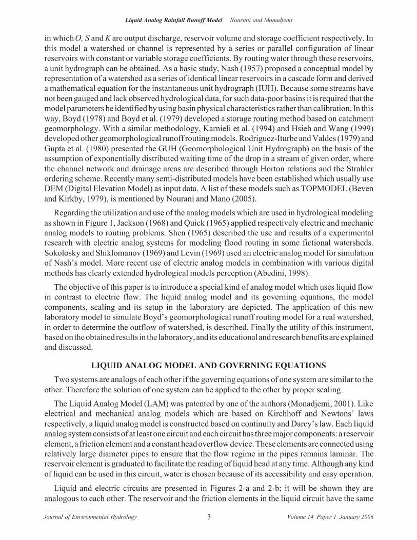
Liquid and electric circuits are presented in Figures 2-a and 2-b; it will be shown they areanalogous to each other. The reservoir and the friction elements in the liquid circuit have the same



roles as the capacitance and resistance in the electric model respectively. Figure 2-c shows a frictionelement of the LAM; this element is built on the basis of water flow through a porous medium(Darcy’s Law). The friction element, in the form of a cylindrical tube, is filled with porous media suchas sand with a hydraulic conductivity of c. The friction element has a length of l and a sectional areaof a. The two ends of the tube are packed by coarse gravel and two screens are also used to separatethe sand and the gravel. Because of the pipes shortness and low flow velocity in them, the frictionand minor head losses are negligible. By applying Darcy’s law, in the laminar flow regime, the flowdischarge through the friction element which has a water head of y is given by:

Q=Va=(ca/l)y=py (2)in which V is flow velocity in the friction element and ca/l is assumed to be constant and equal is top with dimensions of L2/T. Since the reservoir element area, a, is constant, Equation 2 shows a directproportional relation between outflow discharge and reservoir element storage and thus it representsthe linear reservoir concept. The constant head overflow device in the LAM is located above thefriction element to keep the friction element always saturated. It is to be noted that the constant headoverflow device is a separator in the LAM and is mathematically analogous to a unit quotientcoefficient amplifier in an electric analog model (EAM) (Figure 2-b). Using the linear reservoirrelation (Equation 2) and the continuity equation in the following form:

I Q dSdt

A− = (3)

in which Q, I and SA are outflow, inflow and water volume of the LAM reservoir element respectively,the governing differential equation of a liquid analog circuit can be derived:

I QdSdt

Adydt

Adydt

py IAp

dydt

yIp

A− = = → + = → + = (4)

or

Ap

dQdt

Q I+ = (5)

Similarly the governing differential equation of the EAM can be derived using Krichhoff’s lawin the following form:

E E Ri

i C dEdt

Since i then i i E E R C dEdt

1 1

20

3 1 2 10

0− =

=

UV|W|

= = → − =: . (6)

according to an amplifier operation with the quotient coefficient of K0, it follows that:

K E E E E EK0 2 2

02

0− = → =>>b g (7)

by substituting of Equation 7 in Equation 6 the final differential equation will be derived:

R C dEdt

E E. 2

02 1+ = (8)



y0y

p

A

Reservoir Element

Constant HeadOverflow Device

Friction Element

Amplifier

CapacitanceElectricityCurrent

i1

R

C

K1

3

0

2

EE2E

Voltage

ii

Resistance

Figure 2. (a) liquid (b) electric analog circuit (c) friction element of LAM.

a b c

in which E, i, R, C, t0 are voltage, current, resistance, capacitance and time in an electric modelrespectively. Like an electrical circuit in which the amplifier does not allow any current movementbut voltage can move to the other side of the circuit, in a liquid analog circuit, the water head, contraryto water discharge, can not move to the next circuit due to the constant head device. Finally bycombination of Equation 1 and the continuity equation, the following differential equation is derivedfor a conceptual linear reservoir:

K dOdT

O I L+ = (9)

where IL is inflow water discharge to the linear reservoir and T is time in the prototype. The analogyamong the three mentioned systems can be clearly observed by comparison of Equations. 5, 8 and9 with an arbitrary initial condition and the variables A/p, K and R.C are all equivalent

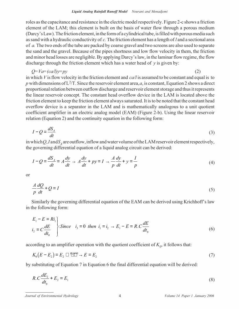
In the EAM, if an annular Krichhoff’s law is used instead of a nodal one, in differential Equation8, current will be expressed as a function of t0 instead of voltage and in this manner for the LAM inEquation 5, the water head rather than water discharge can be expressed as a function of t (Equation4). Like the EAM, several liquid circuits can be combined in series, parallel, cascade, connected orother complex configurations to create a system with a known governing differential equation. Acascade system of two liquid circuits and its electrical analog have been shown in Figure 3. In the

y0y1

y2

A

p

1

2

1

A

2

p

2R

C

1E ER1

1

2

C 2

Figure 3. (a) liquid (b) electric cascade analog.

(a) (b)



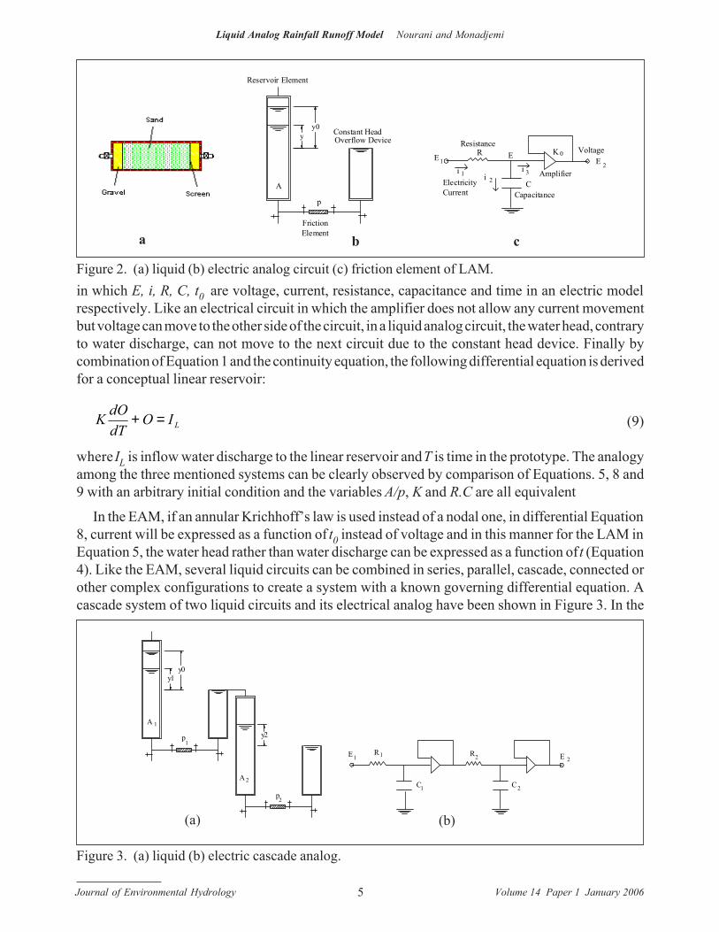
electrical model, if the amplifiers are not used, current can move to the next circuit (Figure 4-b),similarly in the liquid system if liquid circuits (reservoir plus friction elements) are directly connectedtogether (Figure 4-a), the water head in each reservoir will affect the other reservoir; this situationpresents a linear system but with a feedback effect. Referring to Figure 4-a, if the water levels areequal in the reservoir elements, no water discharge will be transferred between reservoirs, howeverif an impulse as a water head or discharge is applied to one of the reservoirs, the water will flow inthe system. Suppose that at time t the water levels in the first reservoir element with cross section A1is y1 and in second reservoir element with cross section area A2 is y2, and the friction coefficients ofthe friction elements and the outflow of the reservoirs are p1, p2, Q1, and Q2, respectively and I (t)is input discharge to the first reservoir element, using Equations 2 and 3 the following equation setcan be written:

Q p y y

I Q A dydt

Q p y

Q Q A dydt

1 1 1 2

1 11

2 2 2

1 2 22

= −

− =

=

− =

R

S|||

T|||

b g

(10)

Each of the four unknown variables (Q1,Q2,y1,y2) can be found by solving the foregoing equationset. The last output discharge (Q2) is of more interest than the others and this variable can be expressedby the following second order ordinary differential equation:

d Qdt

pA

pA

pA

dQdt

p pA A

Q p pA A

I t2

22

1

1

2

2

1

2

2 1 2

1 22

1 2

1 2

+ + +FHG

IKJ + = ( ) (11)

This equation along with any initial conditions defines the behavior of the above system to produceoutput discharge, Q2. The governing differential equation for a liquid cascade system (Figure 3a) willbe similar to Equation 11 but without p1/A2 in the second term. It implies there is no interferencebetween the reservoir elements. By a similar methodology, the governing differential equation for aLAM with n connected reservoir elements is:

y2y1

y0

C

R R

Ci

A

p1 2

1 2

1 2A

p2

1 2

1

i

E

(a) (b)

Figure 4. Connected (a) liquid (b) electric circuits.



[ ( ... )

( ) ( ) ... ( )]

D D

D D QpA

I t

n n

n

n

i j

i j

n

j i

n

i

ni j k

i j k

n

i

ni

ik j

n

j i

n

ni

ni

ii

n

i j

i j

i j k

i j k

+ + + +

+ + + + =

−

−

−

−

= +

−

=≠≠

−−

== +≠ ≠≠ ≠

−

= +

−

==

−

∑∑ ∏∑∑ ∏∑

αβ

αβ

αβ

α αβ β

α α αβ β β

αβ

α αβ β

α α αβ β β

1

1

2

2

2 1

2 1

1

2

1

2 1

1

2 13

11

2 1

1

2 1

11

2 1 a f (12)

where D=d/dt is the differential operator and for

i to npA

i n to npA

i i

i i

i i n

i i n

===

RST = + −==

RST−

− +

0 1 2 11

: :αβ

αβ

and for

For n=2 , this equation changes to Equation 11.

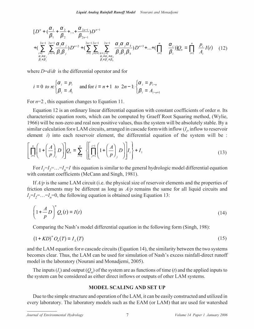
Equation 12 is an ordinary linear differential equation with constant coefficients of order n. Itscharacteristic equation roots, which can be computed by Graeff Root Squaring method, (Wylie,1966) will be non-zero and real non positive values, thus the system will be absolutely stable. By asimilar calculation for n LAM circuits, arranged in cascade form with inflow (Ii, inflow to reservoirelement i) into each reservoir element, the differential equation of the system will be :

1 11 2 1

1

1+FHGIKJ

FHG

IKJ

LNMM

OQPP = +

FHGIKJ

FHG

IKJ

LNMM

OQPP

RS|T|

UV|W|

+= = =

−

∏ ∑ ∏Ap

D Q Ap

D I Iii

n

ni

n

jj

i

i (13)

For I1=I2=…=In=I this equation is similar to the general hydrologic model differential equationwith constant coefficients (McCann and Singh, 1981).

If A/p is the same LAM circuit (i.e. the physical size of reservoir elements and the properties offriction elements may be different as long as A/p remains the same for all liquid circuits andI1=I2=…=In=0, the following equation is obtained using Equation 13:

1+FHG

IKJ =

Ap

D Q t I tn

n a f a f (14)

Comparing the Nash’s model differential equation in the following form (Singh, 198):

1+ =KD O T I Tnn La f a f a f (15)

and the LAM equation for n cascade circuits (Equation 14), the similarity between the two systemsbecomes clear. Thus, the LAM can be used for simulation of Nash’s excess rainfall-direct runoffmodel in the laboratory (Nourani and Monadjemi, 2005).

The inputs (Ii) and output (Qn) of the system are as functions of time (t) and the applied inputs tothe system can be considered as either direct inflows or outputs of other LAM systems.

MODEL SCALING AND SET UP

Due to the simple structure and operation of the LAM, it can be easily constructed and utilized inevery laboratory. The laboratory models such as the EAM (or LAM) that are used for watershed



modeling and study of hydrological laws, watershed response, or creating experimental data arecategorized in the laboratory prototype group and they are different from small-scale physical models(Amorocho and Hart, 1965). The LAM system when acting in a linear form, can be built and utilizedfor multi scaled times and discharges. When each part of a watershed is considered as a linearreservoir with storage coefficient Ki through a conceptual model, every liner reservoir can berepresented by a LAM circuit with proper (A/p)i in the laboratory.

Equation 12 or 13, clearly shows that there are two independent variables, i.e. time and discharge(or head), in a liquid analog system. Therefore, two scale coefficients, time scale and discharge scaleare necessary. Time scale, τ , can be computed by the following ratio:

τ = =( )

, ,...,

ApK

i ni

i

1 2 (16)

and the discharge scale, γ , can be obtained by Equation 17:

γ = II L

max

max

(17)

in which I ILmax, max are the maximum discharge in the real system and the maximum applicable

discharge in the laboratory respectively.

For the scaling and design of the LAM in the laboratory, the following procedure may be followed:

a) The conceptual model parameters (n,Ki) are estimated by any parameters estimation method.

b)A reasonable time scale, τ, is chosen.

c) From Equation 16, (A/p)i are obtained for all Lam circuits.

d) By allocating suitable values to Ai , ai , and li , the values of pi and consequently ci are determinedusing equation 2 e) On the basis of the values ci , the sand in each friction element is prepared by theuse of a permeability meter in a soil mechanics laboratory. It is clear that in the mentioned steps otherparameters can be assumed and the rest can be obtained.

f) Discharge scale, γ , is computed by Equation 17 and then by applying this scale on input dischargesof the real system, the input discharges of laboratory LAM are obtained.

g) the maximum water level in the last reservoir, ymax is approximately obtained by:

Imax=pn ymax (18)In the model design all the parameters are selected in such a way so the reservoir elements do not

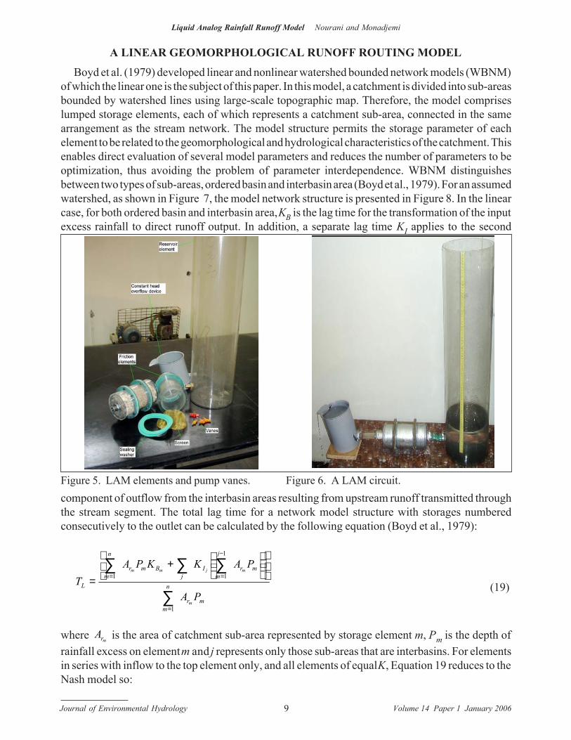
overflow. The different components of the LAM constructed in the laboratory and used for theexperimentation are shown in Figure 5 and a complete LAM circuit is shown in Figure 6. Thecalibration of individual LAM circuits which verifies the linear relation between head and dischargeis strongly recommended. In this way there is no need for the discharge measurement and a simplereading of water head gives the discharge (see Equation 2). After calibration of all the circuits, therequired system, having a particular configuration, will be assembled. The scaled input loads, usingwater, on the system in the form of pulses can be easily applied by several pumps having differentcapacities.



A LINEAR GEOMORPHOLOGICAL RUNOFF ROUTING MODEL

Boyd et al. (1979) developed linear and nonlinear watershed bounded network models (WBNM)of which the linear one is the subject of this paper. In this model, a catchment is divided into sub-areasbounded by watershed lines using large-scale topographic map. Therefore, the model compriseslumped storage elements, each of which represents a catchment sub-area, connected in the samearrangement as the stream network. The model structure permits the storage parameter of eachelement to be related to the geomorphological and hydrological characteristics of the catchment. Thisenables direct evaluation of several model parameters and reduces the number of parameters to beoptimization, thus avoiding the problem of parameter interdependence. WBNM distinguishesbetween two types of sub-areas, ordered basin and interbasin area (Boyd et al., 1979). For an assumedwatershed, as shown in Figure 7, the model network structure is presented in Figure 8. In the linearcase, for both ordered basin and interbasin area, KB is the lag time for the transformation of the inputexcess rainfall to direct runoff output. In addition, a separate lag time KI applies to the second

Figure 5. LAM elements and pump vanes. Figure 6. A LAM circuit.component of outflow from the interbasin areas resulting from upstream runoff transmitted throughthe stream segment. The total lag time for a network model structure with storages numberedconsecutively to the outlet can be calculated by the following equation (Boyd et al., 1979):

mr

n

m

mr

j

mI

jBmr

n

mL

PA

PAKKPAT

m

mjmm

∑

∑∑∑

=

−

==

+

=

1

1

11

(19)

where Arm is the area of catchment sub-area represented by storage element m, Pm is the depth ofrainfall excess on element m and j represents only those sub-areas that are interbasins. For elementsin series with inflow to the top element only, and all elements of equal K, Equation 19 reduces to theNash model so:



TL = nK (20)

A network with ′n ordered basins can be realistically considered as 2 ′n -1 parallel paths in acascade formation which the rainfall takes to arrive at the outlet of the watershed. Therefore the IUHof the model will be the summation of these cascades (Singh, 1988):

( ) ( )i

ji

r

jLILB

n

iT

ATDKDKA

Th δ∏∑ ++

=−′

=

11

)1()1(11 12

1 (21)

where AT is the area of whole basin, Ari is the contributed of the i cascade, nn is the number ofinterbasin areas in the i cascade and DL=d/dT. In Figure 9 all possible paths of the flow, for thewatershed shown in Figure 7, are shown. Boyd et al. (1979) related the storage coefficients and sub-basins area through power functions:

1

1

brGB ii

AaK = (22)

and

2

2

brGI ii

AaK = (23)

where the unit of KB , KI is hours and the unit of Ar is km2. The constant coefficients B2, b1, aG2, aG1

arederived by statistical analysis. In the current study, for simplification of the model, it is assumed thatthe ordered basins coincide with the interbasin areas i.e. K K KB ii i

= =1 . Thus in this case Equation

Outlet

1

2

3

4

5 Ordred Basin

Interbasin A reas53

3

5

5

5

B

IK

K

Figure 7. A watershed divided to sub-basins. Figure 8. Network representation of the watershed.

Figure 9. Cascade representation of the watershed.



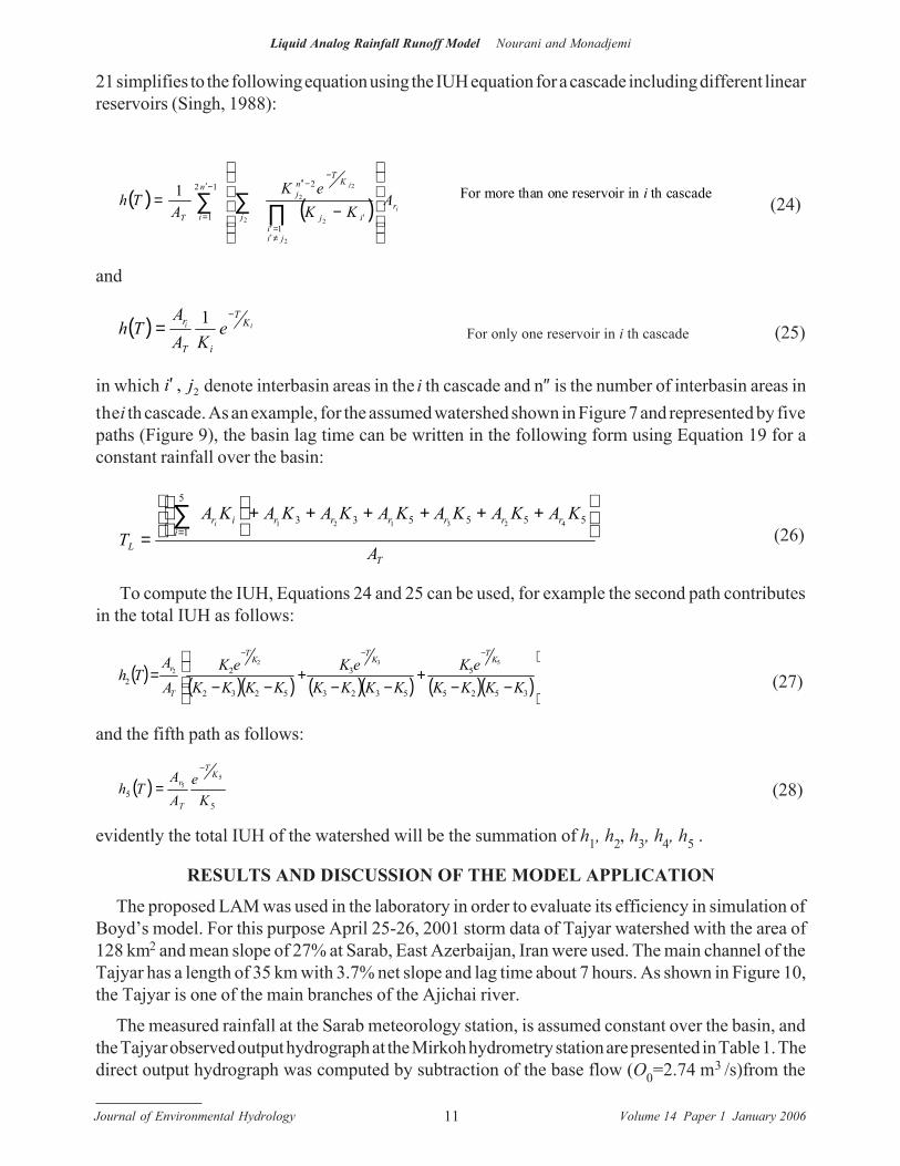
21 simplifies to the following equation using the IUH equation for a cascade including different linearreservoirs (Singh, 1988):

( ) ( ) i

j

rij

jii

KT

nj

j

n

iT

AKK

eKA

Th

−=

′

≠′=′

−−′′−′

= ∏∑∑2

2

2

2

21

212

1

1 For more than one reservoir in i th cascade (24)

and

( ) ii KT

iT

r eKA

ATh

−= 1

For only one reservoir in i th cascade (25)

in which 2, ji′ denote interbasin areas in the i th cascade and n″ is the number of interbasin areas inthe i th cascade. As an example, for the assumed watershed shown in Figure 7 and represented by fivepaths (Figure 9), the basin lag time can be written in the following form using Equation 19 for aconstant rainfall over the basin:

T

rrrrrriri

L A

KAKAKAKAKAKAKAT

i

++++++

=∑

=555533

5

1423121

(26)

To compute the IUH, Equations 24 and 25 can be used, for example the second path contributesin the total IUH as follows:

( ) ( )( ) ( )( ) ( )( )

−−+

−−+

−−=

−−−

3525

5

5323

3

5232

22

5322

KKKKeK

KKKKeK

KKKKeK

AA

ThK

TK

TK

T

T

r

(27)

and the fifth path as follows:

( )5

5

55

Ke

AA

ThK

T

T

r

−

= (28)

evidently the total IUH of the watershed will be the summation of h1, h2, h3, h4, h5 .

RESULTS AND DISCUSSION OF THE MODEL APPLICATION

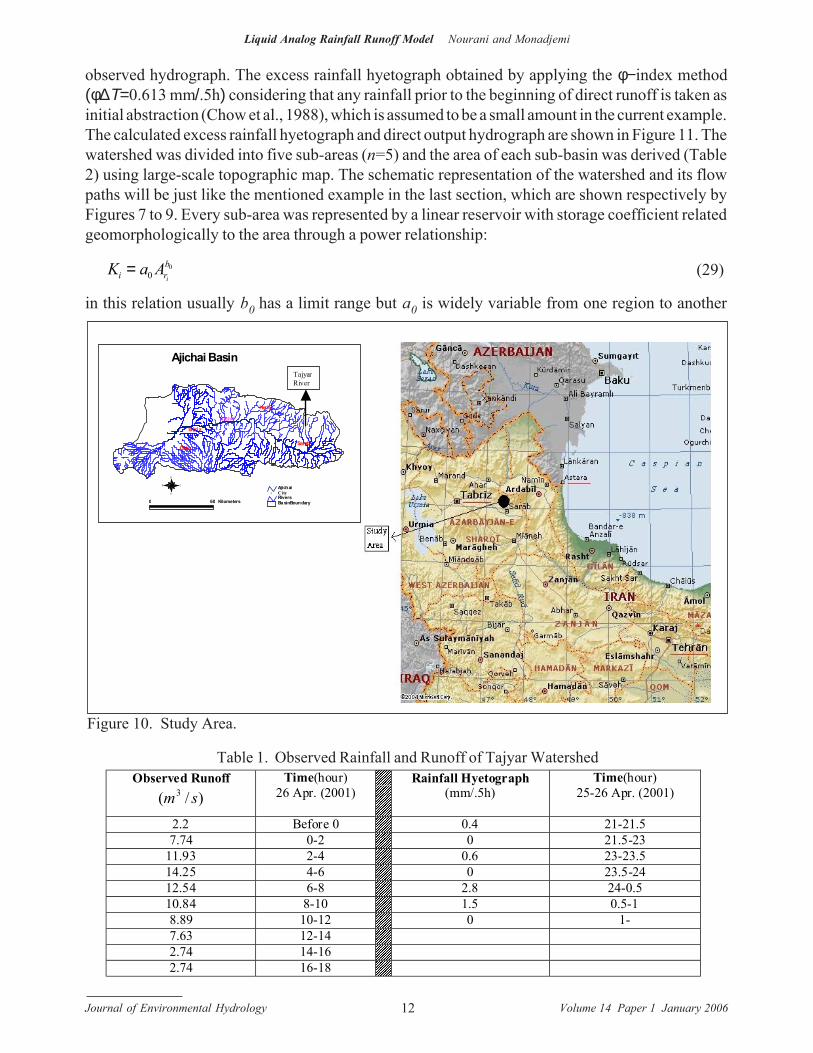
The proposed LAM was used in the laboratory in order to evaluate its efficiency in simulation ofBoyd’s model. For this purpose April 25-26, 2001 storm data of Tajyar watershed with the area of128 km2 and mean slope of 27% at Sarab, East Azerbaijan, Iran were used. The main channel of theTajyar has a length of 35 km with 3.7% net slope and lag time about 7 hours. As shown in Figure 10,the Tajyar is one of the main branches of the Ajichai river.

The measured rainfall at the Sarab meteorology station, is assumed constant over the basin, andthe Tajyar observed output hydrograph at the Mirkoh hydrometry station are presented in Table 1. Thedirect output hydrograph was computed by subtraction of the base flow (O0=2.74 m3 /s)from the



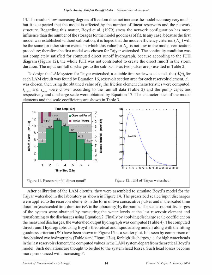
observed hydrograph. The excess rainfall hyetograph obtained by applying the φ−index method(φ∆Τ=0.613 mm/.5h) considering that any rainfall prior to the beginning of direct runoff is taken asinitial abstraction (Chow et al., 1988), which is assumed to be a small amount in the current example.The calculated excess rainfall hyetograph and direct output hydrograph are shown in Figure 11. Thewatershed was divided into five sub-areas (n=5) and the area of each sub-basin was derived (Table2) using large-scale topographic map. The schematic representation of the watershed and its flowpaths will be just like the mentioned example in the last section, which are shown respectively byFigures 7 to 9. Every sub-area was represented by a linear reservoir with storage coefficient relatedgeomorphologically to the area through a power relationship:

K a Ai rbi

= 00 (29)

in this relation usually b0 has a limit range but a0 is widely variable from one region to another

%

%

%

%

Osku

Heris

Sarab

Tabriz

Ajichai

Ba sinBoundaryRivers

% C ityAjichai

0 60 Kilometers

N

EW

S

Ajichai BasinTajyarRiver

Figure 10. Study Area.

Table 1. Observed Rainfall and Runoff of Tajyar WatershedObserved Runoff

)/( 3 smTime(hour)

26 Apr. (2001)

��

Rainfall Hyetograph(mm/.5h)

Time(hour)25-26 Apr. (2001)

2.2 Before 0�� 0.4 21-21.5

7.74 0-2�� 0 21.5-23

11.93 2-4�� 0.6 23-23.5

14.25 4-6

�� 0 23.5-24

12.54 6-8

�� 2.8 24-0.5

10.84 8-10

�� 1.5 0.5-1

8.89 10-12

��

0 1-7.63 12-14

��

2.74 14-16

��

2.74 16-18

��



(Singh, 1988). In the present study b0 was considered equal to 0.38 (Boyd et al., 1979) but a0 wascomputed using lag time. Considering that lag time is equal to the time from the centroid of the excessrainfall hyetograph to the centroid of the direct runoff hydrograph, the whole basin lag was obtained,TL=6.8 hrs, which is approximately equal to the reported lag time (i. e. 7 hrs). Consequently, bysubstituting sub-basin areas (Table 2) into Equation 26 and using Equation 29, a0=0.825 wasobtained for the current example. Thus all parameters (n,Ki) were directly obtained without anyoptimization and are presented in Table 2.

It must be noticed although TL was computed using storm data, it can be considered as ageomorphological characteristic of the watershed and related to the watershed physical propertiesthrough some mathematical equations without any calibration (Singh, 1988). The model IUH wasfound by Equations 24 and 25 as:

h T e e e e eT T T T Ta f = − + − +

− − − − −2 1 4 0 35 017 1723 7 3 2 1 2 14 2 7. . . .. . . . (30)

with inverse hours units and shown in Figure 12.

The linear assumption for any watershed hydrologic system yields a direct runoff given by theconvolution integral in the following matrix form (Singh, 1988):

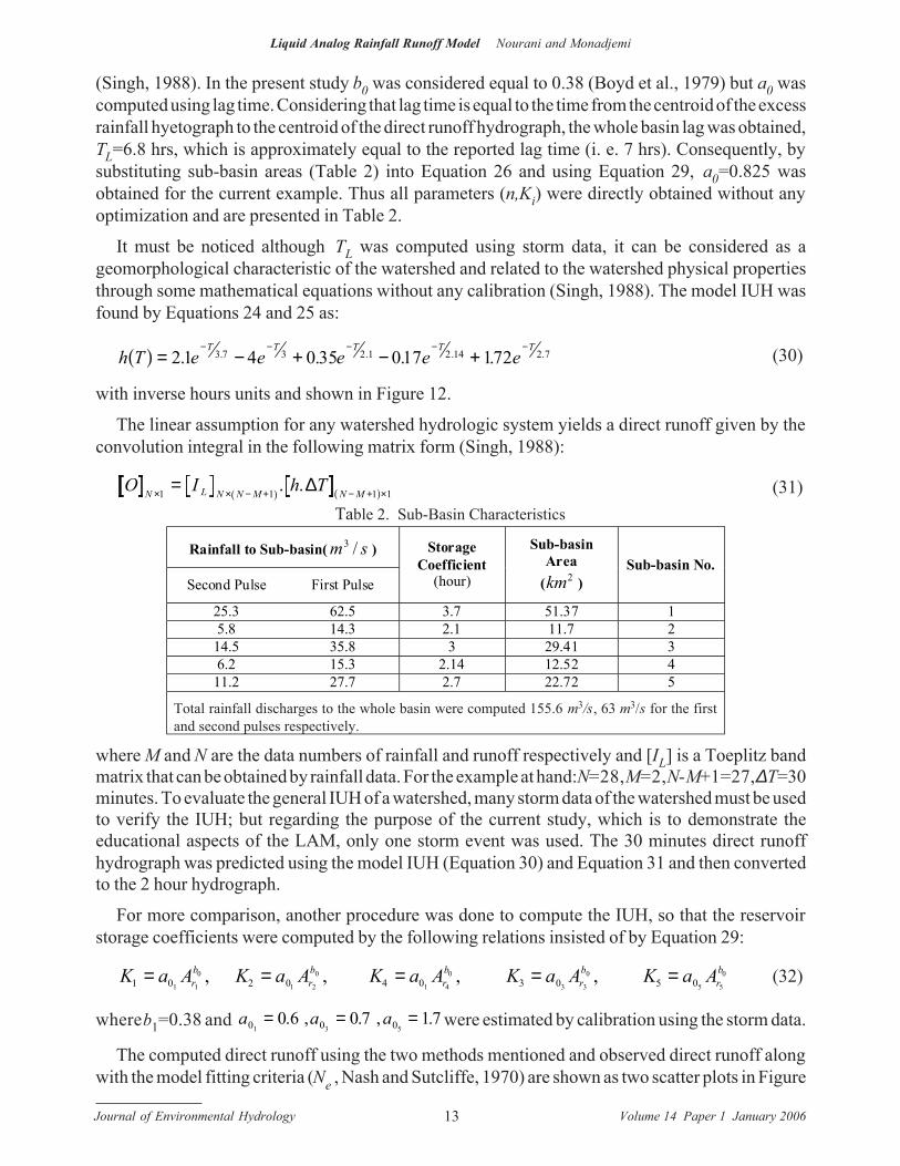
O I h TN L N N M N M× × − + − + ×=1 1 1 1a f a f. .∆ (31)Table 2. Sub-Basin Characteristics

Rainfall to Sub-basin( sm /3 )

Second Pulse First Pulse

StorageCoefficient

(hour)

Sub-basinArea

( 2km )Sub-basin No.

25.3 62.5 3.7 51.37 15.8 14.3 2.1 11.7 214.5 35.8 3 29.41 36.2 15.3 2.14 12.52 411.2 27.7 2.7 22.72 5

Total rainfall discharges to the whole basin were computed 155.6 m3/s, 63 m3/s for the firstand second pulses respectively.

where M and N are the data numbers of rainfall and runoff respectively and [IL] is a Toeplitz bandmatrix that can be obtained by rainfall data. For the example at hand: N=28, M=2, N-M+1=27, ∆T=30minutes. To evaluate the general IUH of a watershed, many storm data of the watershed must be usedto verify the IUH; but regarding the purpose of the current study, which is to demonstrate theeducational aspects of the LAM, only one storm event was used. The 30 minutes direct runoffhydrograph was predicted using the model IUH (Equation 30) and Equation 31 and then convertedto the 2 hour hydrograph.

For more comparison, another procedure was done to compute the IUH, so that the reservoirstorage coefficients were computed by the following relations insisted of by Equation 29:

K a A K a A K a A K a A K a Arb

rb

rb

rb

rb

1 0 2 0 4 0 3 0 5 01 1

0

1 2

0

1 4

0

3 3

0

5 5

0= = = = =, , , , (32)

where b1=0.38 and a a a0 0 01 3 50 6 0 7 17= = =. , . , . were estimated by calibration using the storm data.

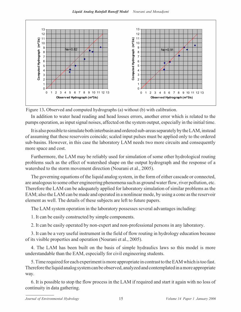
The computed direct runoff using the two methods mentioned and observed direct runoff alongwith the model fitting criteria (Ne , Nash and Sutcliffe, 1970) are shown as two scatter plots in Figure



13. The results show increasing degrees of freedom does not increase the model accuracy very much,but it is expected that the model is affected by the number of linear reservoirs and the networkstructure. Regarding this matter, Boyd et al. (1979) stress the network configuration has moreinfluence than the number of the storages for the model goodness of fit. In any case; because the firstmodel was established without calibration, it is hoped that the model efficiency criterion ( Ne ) willbe the same for other storm events in which this value for Ne is not low in the model verificationprocedure; therefore the first model was chosen for Tajyar watershed. The continuity condition wasnot completely satisfied for computed direct runoff hydrograph, because according to the IUHdiagram (Figure 12), the whole IUH was not contributed to create the direct runoff in the stormduration. The input rainfall discharges to the sub-basins as two pulses are presented in Table 2.

To design the LAM system for Tajyar watershed, a suitable time scale was selected , the (A/p)i foreach LAM circuit was found by Equation 16, reservoir section area for each reservoir element, Ai ,was chosen, then using the obtained value of pi ,the friction element characteristics were computed.ILmax and Imax were chosen according to the rainfall data (Table 2) and the pump capacitiesrespectively and discharge scale were obtained by Equation 17. The characteristics of the modelelements and the scale coefficients are shown in Table 3.

8.1

6.154.9

9.8

11.5

9.2

5

2.187

0.887

0

2

4

6

8

10

12

14

1 2 3 4 5 6 7Time Step (2 h)

Dire

ct R

unof

f (m

^3/s

)

012345678910

Time Step (.5 h)

Exce

ss R

ainf

all

(mm

/.5h)

Observed Runoff

Excess Rainfall

� � � � � ��

��

��

��

��

��

��

��

��

��

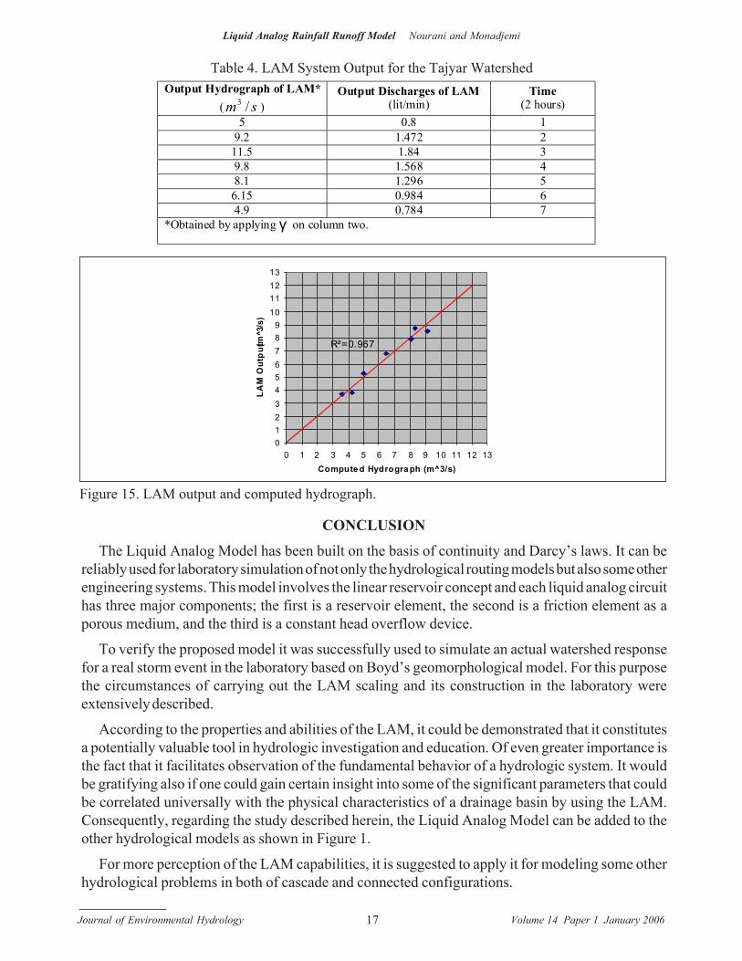
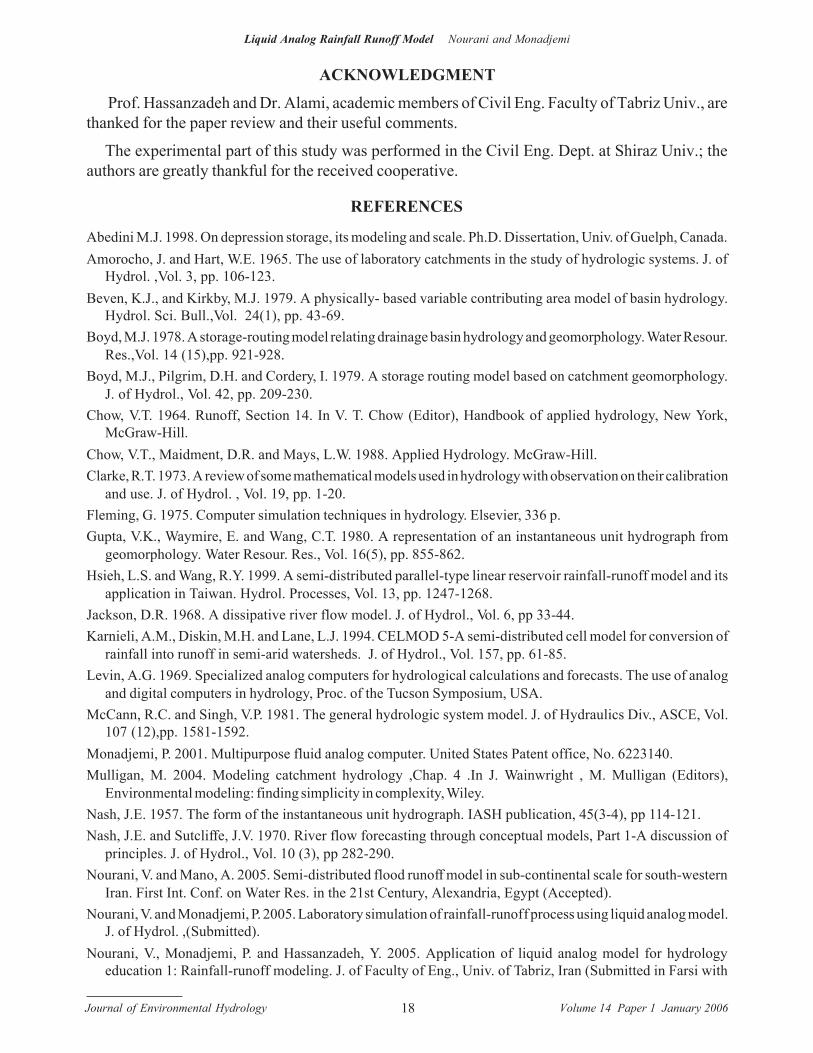
After calibration of the LAM circuits, they were assembled to simulate Boyd’s model for theTajyar watershed in the laboratory as shown in Figure 14. The prescribed scaled input dischargeswere applied to the reservoir elements in the form of two consecutive pulses and in the scaled timeduration (each scaled time duration is ∆t in the laboratory) by the pumps. The scaled output dischargesof the system were obtained by measuring the water levels at the last reservoir element andtransforming to the discharges using Equation 2. Finally by applying discharge scale coefficient onthe measured discharges, the watershed output hydrograph was computed (Table 4). The computeddirect runoff hydrographs using Boyd’s theoretical and liquid analog models along with the fittinggoodness criterion (R2 ) have been shown in Figure 15 as a scatter plot. It is seen by comparison ofthe obtained two hydrographs (Table 4 and Figure 13-a), for high discharges, i.e. for high water headsin the last reservoir element, the computed values in the LAM system depart from theoretical Boyd’smodel. Such deviations are thought to be due to the system head losses. Such head losses becomemore pronounced with increasing V.

Figure 11. Excess rainfall direct runoff Figure 12. IUH of Tajyar watershed



In addition to water head reading and head losses errors, another error which is related to thepumps operation, as input signal noises, affected on the system output, especially in the initial time.

It is also possible to simulate both interbasin and ordered sub-areas separately by the LAM, insteadof assuming that these reservoirs coincide; scaled input pulses must be applied only to the orderedsub-basins. However, in this case the laboratory LAM needs two more circuits and consequentlymore space and cost.

Furthermore, the LAM may be reliably used for simulation of some other hydrological routingproblems such as the effect of watershed shape on the output hydrograph and the response of awatershed to the storm movement direction (Nourani et al., 2005).

The governing equations of the liquid analog system, in the form of either cascade or connected,are analogous to some other engineering phenomena such as ground water flow, river pollution, etc.Therefore the LAM can be adequately applied for laboratory simulation of similar problems as theEAM; also the LAM can be made and operated in a nonlinear mode, by using a cone as the reservoirelement as well. The details of these subjects are left to future papers.

The LAM system operation in the laboratory possesses several advantages including:

1. It can be easily constructed by simple components.

2. It can be easily operated by non-expert and non-professional persons in any laboratory.

3. It can be a very useful instrument in the field of flow routing in hydrology education becauseof its visible properties and operation (Nourani et al., 2005).

4. The LAM has been built on the basis of simple hydraulics laws so this model is moreunderstandable than the EAM, especially for civil engineering students.

5. Time required for each experiment is more appropriate in contrast to the EAM which is too fast.Therefore the liquid analog system can be observed, analyzed and contemplated in a more appropriateway.

6. It is possible to stop the flow process in the LAM if required and start it again with no loss ofcontinuity in data gathering.

0123456789

10111213

0 1 2 3 4 5 6 7 8 9 10 11 12 13Observed Hydrograph (m 3̂/s)

Com

pute

d Hy

drog

raph

(m

^3/s

)

Ne=0.82

0123456789

10111213

0 1 2 3 4 5 6 7 8 9 10 11 12 13Observed Hydrograph (m^3/s)

Com

pute

d Hy

drog

raph

(m

^3/s

)

Ne=0.91

Figure 13. Observed and computed hydrographs (a) without (b) with calibration.



Input toLAM**(lit/min)

pulse2 nd

pulse1 th

Reservoirelementsectionarea(A)

)( 2m

Hydraulicconductivity of

frictionelement(c)

( sm / )

Frictionelementsectionarea(a)

)( 2m

Length offriction

element*(l)(m)

CircuitNo.

4.05 10 0.038 0.0054 0.0095 0.165 10.93 2.3 0.0314 0.0054 0.00785 0.095 22.3 2.7 0.038 0.0054 0.00785 0.11 31 2.45 0.038 0.0054 0.00785 0.08 4

1.8 4.43 0.038 0.0054 0.0095 0.12 5

*According time scale (109

1=τ ) il were computed by assuming other variables using Eq. 16.

**Each pulse in laboratory was 1091800

109=∆=∆ Tt s

- smI L /5.62 3max

= in prototype and min/10max litI = in the laboratory so discharge

scale was375000

1=γ

Table 3. LAM and Input Load Characteristics

On the other hand there are some disadvantages in the LAM including:1. More space and cost needs compared to the EAM.2. Less accuracy due to the existence of head losses and other experimental errors in comparison

with the EAM.3. Less flexibility than the EAM, because some elements of the EAM have not been yet simulated

for the LAM.It is hoped that the LAM system for runoff simulation will be used as a laboratory device in the

future.

Figure 14. Constructed LAM in laboratory for Tajyar watershed.



CONCLUSION

The Liquid Analog Model has been built on the basis of continuity and Darcy’s laws. It can bereliably used for laboratory simulation of not only the hydrological routing models but also some otherengineering systems. This model involves the linear reservoir concept and each liquid analog circuithas three major components; the first is a reservoir element, the second is a friction element as aporous medium, and the third is a constant head overflow device.

To verify the proposed model it was successfully used to simulate an actual watershed responsefor a real storm event in the laboratory based on Boyd’s geomorphological model. For this purposethe circumstances of carrying out the LAM scaling and its construction in the laboratory wereextensively described.

According to the properties and abilities of the LAM, it could be demonstrated that it constitutesa potentially valuable tool in hydrologic investigation and education. Of even greater importance isthe fact that it facilitates observation of the fundamental behavior of a hydrologic system. It wouldbe gratifying also if one could gain certain insight into some of the significant parameters that couldbe correlated universally with the physical characteristics of a drainage basin by using the LAM.Consequently, regarding the study described herein, the Liquid Analog Model can be added to theother hydrological models as shown in Figure 1.

For more perception of the LAM capabilities, it is suggested to apply it for modeling some otherhydrological problems in both of cascade and connected configurations.

Output Hydrograph of LAM*( sm /3 )

Output Discharges of LAM(lit/min)

Time(2 hours)

5 0.8 19.2 1.472 211.5 1.84 39.8 1.568 48.1 1.296 56.15 0.984 64.9 0.784 7

*Obtained by applying γ on column two.

Table 4. LAM System Output for the Tajyar Watershed

0123456789

10111213

0 1 2 3 4 5 6 7 8 9 10 11 12 13Compute d Hydrogra ph (m^3/s)

LA

M O

utp

ut (m

3̂/s)

R²=0.967

Figure 15. LAM output and computed hydrograph.



ACKNOWLEDGMENT

Prof. Hassanzadeh and Dr. Alami, academic members of Civil Eng. Faculty of Tabriz Univ., arethanked for the paper review and their useful comments.

The experimental part of this study was performed in the Civil Eng. Dept. at Shiraz Univ.; theauthors are greatly thankful for the received cooperative.

REFERENCES

Abedini M.J. 1998. On depression storage, its modeling and scale. Ph.D. Dissertation, Univ. of Guelph, Canada.Amorocho, J. and Hart, W.E. 1965. The use of laboratory catchments in the study of hydrologic systems. J. of

Hydrol. ,Vol. 3, pp. 106-123.Beven, K.J., and Kirkby, M.J. 1979. A physically- based variable contributing area model of basin hydrology.

Hydrol. Sci. Bull.,Vol. 24(1), pp. 43-69.Boyd, M.J. 1978. A storage-routing model relating drainage basin hydrology and geomorphology. Water Resour.

Res.,Vol. 14 (15),pp. 921-928.Boyd, M.J., Pilgrim, D.H. and Cordery, I. 1979. A storage routing model based on catchment geomorphology.

J. of Hydrol., Vol. 42, pp. 209-230.Chow, V.T. 1964. Runoff, Section 14. In V. T. Chow (Editor), Handbook of applied hydrology, New York,

McGraw-Hill.Chow, V.T., Maidment, D.R. and Mays, L.W. 1988. Applied Hydrology. McGraw-Hill.Clarke, R.T. 1973. A review of some mathematical models used in hydrology with observation on their calibration

and use. J. of Hydrol. , Vol. 19, pp. 1-20.Fleming, G. 1975. Computer simulation techniques in hydrology. Elsevier, 336 p.Gupta, V.K., Waymire, E. and Wang, C.T. 1980. A representation of an instantaneous unit hydrograph from

geomorphology. Water Resour. Res., Vol. 16(5), pp. 855-862.Hsieh, L.S. and Wang, R.Y. 1999. A semi-distributed parallel-type linear reservoir rainfall-runoff model and its

application in Taiwan. Hydrol. Processes, Vol. 13, pp. 1247-1268.Jackson, D.R. 1968. A dissipative river flow model. J. of Hydrol., Vol. 6, pp 33-44.Karnieli, A.M., Diskin, M.H. and Lane, L.J. 1994. CELMOD 5-A semi-distributed cell model for conversion of

rainfall into runoff in semi-arid watersheds. J. of Hydrol., Vol. 157, pp. 61-85.Levin, A.G. 1969. Specialized analog computers for hydrological calculations and forecasts. The use of analog

and digital computers in hydrology, Proc. of the Tucson Symposium, USA.McCann, R.C. and Singh, V.P. 1981. The general hydrologic system model. J. of Hydraulics Div., ASCE, Vol.

107 (12),pp. 1581-1592.Monadjemi, P. 2001. Multipurpose fluid analog computer. United States Patent office, No. 6223140.Mulligan, M. 2004. Modeling catchment hydrology ,Chap. 4 .In J. Wainwright , M. Mulligan (Editors),

Environmental modeling: finding simplicity in complexity, Wiley.Nash, J.E. 1957. The form of the instantaneous unit hydrograph. IASH publication, 45(3-4), pp 114-121.Nash, J.E. and Sutcliffe, J.V. 1970. River flow forecasting through conceptual models, Part 1-A discussion of

principles. J. of Hydrol., Vol. 10 (3), pp 282-290.Nourani, V. and Mano, A. 2005. Semi-distributed flood runoff model in sub-continental scale for south-western

Iran. First Int. Conf. on Water Res. in the 21st Century, Alexandria, Egypt (Accepted).Nourani, V. and Monadjemi, P. 2005. Laboratory simulation of rainfall-runoff process using liquid analog model.

J. of Hydrol. ,(Submitted).Nourani, V., Monadjemi, P. and Hassanzadeh, Y. 2005. Application of liquid analog model for hydrology

education 1: Rainfall-runoff modeling. J. of Faculty of Eng., Univ. of Tabriz, Iran (Submitted in Farsi with



English abstract).Quick, M.C. 1965. River flood flows: forecasts and probabilities. J. of Hydraulics Div., ASCE, Vol. 91 (HY3),

pp 1-17.Rodriguez-Iturbe, I. and Valdes, J.B. 1979. The geomorphologic structure of hydrologic response. Water Resour.

Res., Vol. 15 (6),pp. 1409-1420.Shen, J. 1965. Use of analog models in the analysis of flood runoff. Geological survey professional paper 506-

A, U. S. Department of Interior, Washington, D. C.Singh, V.P. 1988. Hydrological Systems, Vol. 1: Rainfall-Runoff Modeling. Prentice Hall, Englewood Cliffs, NJ.

ADDRESS FOR CORRESPONDENCEVahid NouraniFaculty of Civil EngineeringTabriz UniversityTabriz, Iran

Email:[email protected]

journal of environmental hydrology · mathematical methods in hydrology physical/deterministic...

Documents