ARTICLE IN PRESS

Contents lists available at ScienceDirect

Journal of Financial Economics

Journal of Financial Economics 92 (2009) 153–181

0304-40

doi:10.1

$ We

Hasbrou

Yu, and

Finance

Charles

respons� Cor

E-m

journal homepage: www.elsevier.com/locate/jfec

Do liquidity measures measure liquidity?$

Ruslan Y. Goyenko a, Craig W. Holden b, Charles A. Trzcinka b,�

a Desautels Faculty of Management, McGill University, Montreal, Quebec, Canada H3A 1G5b Kelley School of Business, Indiana University, 1309 East Tenth Street, Bloomington, IN 47405-1701, USA

a r t i c l e i n f o

Article history:

Received 21 February 2005

Received in revised form

25 February 2008

Accepted 9 June 2008Available online 3 February 2009

JEL classifications:

C15

G12

G20

Keywords:

Liquidity

Transaction costs

Effective spread

Price impact

Asset pricing

5X/$ - see front matter & 2009 Published by

016/j.jfineco.2008.06.002

thank Utpal Bhattacharya, Andrew Ellul,

ck, Christian Lundblad, Darius Miller, Marios

seminar participants at Indiana University a

Conference in Bonaire, Netherlands Antill

Jones for making Dow spreads availabl

ible for any errors.

responding author. Tel.: +1812 855 9908; fax:

ail address: ctrzcink@indiana.edu (C.A. Trzcin

a b s t r a c t

Given the key role of liquidity in finance research, identifying high quality proxies based

on daily (as opposed to intraday) data would permit liquidity to be studied over

relatively long timeframes and across many countries. Using new measures and widely

employed measures in the literature, we run horseraces of annual and monthly

estimates of each measure against liquidity benchmarks. Our benchmarks are effective

spread, realized spread, and price impact based on both Trade and Quote (TAQ) and Rule

605 data. We find that the new effective/realized spread measures win the majority of

horseraces, while the Amihud [2002. Illiquidity and stock returns: cross-section and

time-series effects. Journal of Financial Markets 5, 31–56] measure does well measuring

price impact.

& 2009 Published by Elsevier B.V.

1. Introduction

The role of liquidity in empirical finance has grownrapidly over the past five years influencing conclusions inasset pricing, market efficiency, and corporate finance. Anumber of studies have proposed liquidity measuresderived from daily return and volume data as proxies forinvestors’ liquidity and transaction costs. These studiesusually test whether security returns are related to theseliquidity measures but rarely test whether the measuresare related to actual transaction costs. The assumption

Elsevier B.V.

Jaden Falcone, Joel

Panayides, Xiaoyun

nd the Frontiers of

es. We also thank

e. We are solely

+1812 855 5875.

ka).

that the available liquidity proxies capture the transactioncosts of market participants is often not tested because ofthe limited availability of actual trading costs. In the USmarkets transaction data are only available since 1983 andin many countries transaction data are not available at all.The consequences of not testing liquidity proxies on actualtrading data is that there is little consensus on whichmeasures are better and little evidence that any of theproposed measures are related to investor experience.

Further, while a handful of studies, Lesmond, Ogden,and Trzcinka (1999), Lesmond (2005), and Hasbrouck(2009), test whether some of the available liquidityproxies are related to liquidity benchmarks computedfrom transaction data, they construct the liquidity proxieson an annual or quarterly basis. Yet the vast majority ofthe literature using liquidity proxies employs them onmonthly (or finer) data. Given the limited number ofliquidity proxies previously tested, the limited set ofliquidity benchmarks used in the literature, and theabsence of monthly proxies, it is not surprising that there

ARTICLE IN PRESS

R.Y. Goyenko et al. / Journal of Financial Economics 92 (2009) 153–181154

are conflicting views about which measure is betterand that there is little assurance that these measuresactually capture the transaction costs of market partici-pants. In short, not much is known about whethertransaction cost proxies measure what researchers claimthey measure.

The purpose of this paper is to address this gap in theliterature by providing a comprehensive study of liquiditymeasures. We run ‘‘horseraces’’ of all the widely usedproxies for liquidity, plus three new proxies for effectiveand realized spread, and nine new proxies for priceimpact. We use multiple liquidity benchmarks, twohigh-frequency data sets (TAQ and Rule 605 data), multi-ple performance metrics, and a long sample period thatincludes the decimals regime.

We find a close association between many of themeasures and actual transaction costs. Some measures areable to precisely estimate the magnitude of effective andrealized spreads and many are highly correlated with bothspreads and price impact. We can safely assert that theliterature has generally not been mistaken in the assump-tion that liquidity proxies measure liquidity. The newmeasures we introduce in this paper consistently win amajority of the effective/realized spread horseraces. Ameasure commonly used in the literature, Pastor andStambaugh’s (2003) Gamma, is clearly dominated byother measures while the widely used Amihud (2002)measure is a good proxy for price impact.

The paper is organized as follows. Section 2 discussesthe empirical design of the paper. In Section 3 we developthe high-frequency liquidity benchmarks used in thehorserace and in Sections 4 and 5 we develop the low-frequency spread proxies and price impact proxies used inthe horserace. Section 6 describes the data sets andmethodology. Section 7 presents the horserace results.Section 8 concludes the paper.

1 BBO means the best bid and offer. It is the highest bid and lowest

ask available for a given stock at a moment in time.

2. Empirical design

Our basic hypothesis is that useful monthly and annualliquidity measures can be constructed from low-fre-quency (daily) stock returns and volume data, givingresearchers an access to liquidity measures over a longprice history and in many markets. The US daily stockreturns and volume data are available from the Center forResearch in Security Prices (CRSP) covering NYSE/AMEXfirms from 1926 to the present and NASDAQ firms from1983 to the present. A wide variety of vendors providedaily stock returns and volume data for internationalequity markets. For example, Thomson Financial’s Data-stream provides daily stock returns and volumes coveringfirms in more than 60 countries from 1994 to the presentand daily stock returns for several developed marketsgoing back to the early 1970s.

These tests should be of interest to a broad spectrum ofempirical research in financial economics. In the assetpricing literature, Chordia, Roll, and Subrahmanyam(2000) show that various spread measures vary system-atically. Goyenko (2006) shows that various spreadmeasures are priced. Sadka (2006), Acharya and Pedersen

(2005), Pastor and Stambaugh (2003), and Watanabe andWatanabe (2006) show that various price impact mea-sures are priced. Fujimoto (2003), Korajczyk and Sadka(2008), Hasbrouck (2009), and others test the pricing ofboth spread and price impact measures in the US whileBekaert, Harvey, and Lundblad (2007) test the measures inemerging markets where liquidity concerns may be morepronounced. All of these studies use monthly liquidityestimates. Reliable monthly spread and price impactmeasures going back in time and/or across countries areneeded to determine if these asset pricing relationshipshold up. In the market efficiency literature, De Bondt andThaler (1985), Jegadeesh and Titman (1993, 2001), Chan,Jegadeesh, and Lakonishok (1996), Rouwenhorst (1998),and many others have found monthly trading strategiesthat appear to generate significant abnormal returns. Yet,Chordia, Goyal, Sadka, Sadka, and Shivakumar (2008)show that one of the oldest trading strategies in theliterature, the post earnings announcement drift, cannotproduce returns greater than the Keim and Madhavan(1997) measures. Clearly liquidity measures over timeand/or across countries are needed in order to determineif these trading strategies are truly profitable net of arelatively precise measure of cost of trading.

Finally there is a growing need in corporate financeresearch for useful monthly liquidity measures. Kalev,Pham, and Steen (2003), Dennis and Strickland (2003),Cao, Field, and Hanka (2004), Lipson and Mortal (2004a),Schrand and Verrecchia (2004), Lesmond, O’Connor, andSenbet (2008), and many others examine the impact ofcorporate finance events on stock liquidity. Helfin andShaw (2000), Lipson and Mortal (2004b), Lerner andSchoar (2004), and many others examine the influence ofliquidity on capital structure, security issuance form, andother corporate finance decisions. Liquidity measures overa longer period of time would expand the potentialsample size of this literature. Liquidity measures acrossmany additional countries would greatly extend thepotential diversity of international corporate financeenvironments that this literature could analyze.

To determine which liquidity measures are best, wecompare proxies calculated from low-frequency data tosophisticated benchmarks of liquidity calculated from twohigh-frequency data sets using time-series correlations,cross-sectional correlations, and prediction errors. Speci-fically, we compare spread proxies to effective andrealized spreads and we compare price impact proxies totwo price impact benchmarks. All four of these bench-marks are calculated using the NYSE’s Trade and Quote(TAQ) data set from 1993 to 2005. Our monthly bench-marks are computed as monthly averages based on everytrade and corresponding BBO1 quote over the month andour annual benchmarks are computed as annual averagesbased on every trade and corresponding BBO quote overthe year. We also compare spread proxies to the effective

ARTICLE IN PRESS

R.Y. Goyenko et al. / Journal of Financial Economics 92 (2009) 153–181 155

spread for marketable orders2 and compare price impactproxies to the price impact across order sizes.3 Both ofthese benchmarks are calculated using data disclosedunder Securities and Exchange Commission (SEC) Rule605 of Regulation NMS (formerly Regulation 11Ac1-5)from October 2001 to December 2005. Rule 605 requiresthat all exchanges and other market centers disclosedetailed order-based performance statistics by stock,order type, and order size, providing a cross-check to theTAQ based results.

Our tests consist of running monthly and annualhorseraces between 12 spread proxies and 12 price impactproxies, gauging their abilities to match the salientfeatures of our high-frequency-based benchmarks. Whilesome contestants are well established in the literature,many are being tested for the first time. The new spreadproxies (described in detail below) are: ‘‘Effective Tick,’’and ‘‘Effective Tick2,’’ developed jointly by this paper andHolden (2009); ‘‘Holden’’ from Holden (2009); and ‘‘LOTY-split’’ developed by this paper. The other spread proxiesfrom the previous literature are: ‘‘Roll’’ from Roll(1984); ‘‘Gibbs’’ from Hasbrouck (2004); ‘‘LOT Mixed,’’‘‘Zeros,’’ and ‘‘Zeros2’’ from Lesmond, Ogden, and Trzcinka(1999); ‘‘Amihud’’ from Amihud (2002); ‘‘Pastor andStambaugh’’ from Pastor and Stambaugh (2003); andfinally ‘‘Amivest Liquidity.’’4 The latter three measures arealso tested on price impact dimension. The other nineprice impact contestants (also described below) aredeveloped by this paper as extensions of the Amihudmeasure.

Our first performance metric is the average cross-sectional correlation based on individual firms betweenthe low-frequency liquidity proxy and the high-frequencyliquidity benchmark (effective spread, realized spread, orone of the price impact benchmarks). Our secondperformance metric is the time-series correlation basedon an equally weighted portfolio between the liquidityproxy and the liquidity benchmark. Both of theseperformance metrics are most relevant for asset pricingpurposes, where the magnitude of the correlation,not the scale of the low-frequency proxy, matters. Ourthird and fourth performance metrics are the predictionerror between the liquidity proxy and the liquiditybenchmark as measured by mean bias and the rootmean squared error, respectively. These metrics aremost relevant for market efficiency and corporate financetests, where the scale of the proxy does matter as onewishes to subtract a correctly scaled proxy for transactioncosts.

Hasbrouck (2009) runs annual tests between foureffective cost measures, comparing each to effective

2 Marketable orders are a combination of market orders and

marketable limit orders.3 Defined as the difference in the effective spread between large and

small orders divided by the difference in the average share size between

large and small orders.4 The Amihud, Pastor and Stambaugh, and Amivest measures are

perhaps more naturally thought of as price impact measures, but the use

of these measures in the literature has been more broadly and loosely

justified. Therefore, we test these measures relative to both effective

spread and price impact benchmarks.

spread and price impact computed from TAQ data forthe 1993 to 2005 period. Among the measures he tests,Gibbs dominates as a proxy for annual effective spreadand Illiquidity dominates as a proxy for annual priceimpact.5 Using three annual measures, Lesmond, Ogden,and Trzcinka (1999) find that LOT dominates Roll andZeros. Lesmond (2005) runs quarterly horseraces betweenfive liquidity measures for 23 emerging countries, andfinds that LOT dominates Roll, Illiquidity, Liquidity, andTurnover.

We generally conclude that liquidity measures basedon daily data provide good measures of high-frequencytransaction cost benchmarks (i.e., liquidity measures domeasure liquidity). In the monthly and annual effectiveand realized spread horseraces, we find that Holden,Effective Tick, and LOT Y-split are the best overall. We alsofind that in more recent years, during the decimalsregime, the performance of all measures deteriorates withthe exception of Zeros and the Amihud measures. In theprice impact horseraces, the new class of price impactmeasures introduced in this paper either marginallydominate the Amihud measure or is insignificantlydifferent from it, depending on the benchmark. The newclass of price impact measures is also able to capture themagnitude of the special Rule 605 version of price impact.Pastor and Stambaugh’s Gamma and Amivest’s Liquidityare never in the winning group of any horserace and havevery low association with the six liquidity benchmarksanalyzed.

3. High-frequency liquidity benchmarks

3.1. Spread benchmarks

We analyze three spread benchmarks. Our first spreadbenchmark is the effective spread as calculated from thehigh-frequency TAQ database. Specifically, for a givenstock, the TAQ effective spread on the kth trade is definedas

Effective Spread ðTAQ Þk ¼ 2 � j lnðPkÞ � lnðMkÞj, (1)

where Pk is the price of the kth trade and Mk is themidpoint of the consolidated BBO prevailing at the time of

the kth trade. Aggregating over a time interval i (either amonth or a year), a stock’s Effective Spread (TAQ)i is thedollar-volume-weighted average of Effective Spread(TAQ)k computed over all trades in time interval i.

Our second spread benchmark is the realized spreadfrom Huang and Stoll (1996), which is the temporarycomponent of the effective spread. Specifically, for a given

5 Hasbrouck extends his basic model to include a latent common

liquidity factor for a subsample of stocks. He also estimates his Gibbs

measure for all common NYSE/AMEX/NASDAQ stocks from 1927 to 2005

and tests whether liquidity is a priced risk factor.

ARTICLE IN PRESS

7 There are downsides to 605 data as well. An order that is re-routed

between market centers is double-counted. Further, the 605 data do not

R.Y. Goyenko et al. / Journal of Financial Economics 92 (2009) 153–181156

stock, the TAQ realized spread on the kth trade is definedas

Realized Spread ðTAQ Þk

¼2 � ðlnðPkÞ � lnðPkþ5ÞÞ when the kth trade is a buy

2 � ðlnðPkþ5Þ � lnðPkÞÞ when the kth trade is a sell;

(

(2)

where P(k+5) is the price of trade five-minutes after the kthtrade. The trades are signed according to the Lee andReady (1991) algorithm. Aggregating over a time interval i

(either a month or a year), a stock’s Realized Spread (TAQ)k

is the dollar-volume-weighted average of Realized Spread(TAQ)k computed over all trades in time interval i.

Our third spread benchmark is the effective spread asaggregated from the Rule 605 database. Specifically, for agiven stock, the Rule 605 dollar effective spread based onthe trade generated by the kth order is defined as

$Effective Spread ð605Þk

¼2 � ðPk �mkÞ for marketable buys

2 � ðmk � PkÞ for marketable sells;

((3)

where mk is the midpoint of the consolidated BBOprevailing at the time of receipt of the kth order at theexchange.6 Aggregating over month i, a stock’s EffectiveSpread (605)i is the share-volume-weighted average of$Effective Spread (605)k computed over all market centers(spanning all trades) in month i divided by Pi, the averageprice in month i.

In principle, Effective Spread (605)i should be animprovement over Effective Spread (TAQ)i, as each marketcenter constructs their Rule 605 figures from order data,which are more refined than trade and quote data forseveral reasons. First, the Rule 605 midpoint is based onan order’s time of receipt, whereas a TAQ midpoint is basedon the trade’s time of execution—an order’s time ofreceipt is a closer proxy to the trader’s information set atthe time of order submission. Second, there is noconfusion in the Rule 605 data about buys vs. sells orabout marketable orders vs. non-marketable orderswhereas Lee and Radhakrishna (2000) report that theLee and Ready (1991) method commonly used with TAQdata incorrectly classifies 24% of inside-the-spread tradesthat have a clear trade initiator. Third, there is noconfusion in the Rule 605 data when a marketable buyis crossed with a marketable sell. Lee and Radhakrishna(2000) find that 40% of the trades in their NYSE Trades,Orders, Reports, and Quotes (TORQ) sample are ‘‘nondir-ectional’’ trades, where a marketable buy and marketablesell are crossed. The Rule 605 data correctly treats thiscase as two marketable executions (both a marketable buyexecution and a marketable sell execution). By contrast,users of TAQ data cannot distinguish nondirectional tradesvs. directional trades and usually treat this case as a single

6 Marketable buys are market buy orders and marketable limit buy

orders. Marketable sells are market sell orders and marketable limit sell

orders. Effective spreads are not reported for non-marketable limit

orders in the 605 data.

execution.7 Accordingly, the Rule 605 data provide auseful cross-check to the TAQ-based results; however, theRule 605 data are only available from mid-2001, so thecomparison is limited to only 51 months in our sample.

3.2. Price impact benchmarks

Based upon the literature, we analyze three differentprice impact benchmarks. A static version of price impactis the slope of the price function at a moment in time.Essentially, this is the cost of demanding additionalinstantaneous liquidity and can be thought of as the firstderivative of the effective spread with respect to ordersize. Our first price impact benchmark uses two (aggre-gated) points on this curve to measure the slope.Specifically, for a given stock, the static price impactbased on Rule 605 data over time interval i is

Static Price Impact ð605Þi

¼

ð$Effective Spread ð605ÞBig Orders;i=PiÞ

�ð$Effective Spread ð605ÞSmall Orders;i=PiÞ

24

35

=ðAve Trade Size ð605ÞBig Orders;iÞ

�ðAve Trade Size ð605ÞSmall Orders;iÞ

" #, (4)

where Big Orders, i is the set of all orders in the range of2000–9999 shares that execute in time interval i andsmall Orders, i is the set of all orders in the range of100–499 shares that execute in time interval i.

Our second price impact benchmark introduces a timedimension that is not present in Static Price Impact. Five-minute price impact measures the derivative of the cost ofdemanding a certain amount of liquidity over five minuteswhich may be very different from the analogous curve fordemanding the same amount of liquidity immediately. Inconstructing this measure, we follow Hasbrouck (2009)and calculate the price impact as the slope coefficientl(TAQ) of the regression

rn ¼ lðTAQ Þ � Sn þ un, (5)

where for the nth five-minute period,8 rn is the stockreturn, Sn is the signed square-root dollar volume, that is,

Sn ¼P

ksignðvknÞ

ffiffiffiffiffiffiffiffiffiffivkn

�� ��q, vkn is the signed dollar volume of

the kth trade in the nth five-minute period, and un is theerror term.

Our third price impact benchmark focuses on thechange in quote midpoint after a signed trade. Priceimpact is commonly defined as the increase (decrease) inthe midpoint over a five-minute interval beginning at thetime of the buyer- (seller-) initiated transaction. This is thepermanent price change of a given transaction, orequivalently, the permanent component of the effective

include block trades. The SEC is therefore an imperfect monitor of data

quality. For more discussion of these issues, see Boehmer, Jennings, and

Wei (2003).8 We also tested a 15-minute interval with similar results, suggest-

ing that our results are independent of the time interval over which we

aggregate the data.

ARTICLE IN PRESS

R.Y. Goyenko et al. / Journal of Financial Economics 92 (2009) 153–181 157

spread. Specifically, for a given stock, the TAQ five-minuteprice impact aggregated over a time interval i is

5-Minute Price Impact ðTAQ Þk

¼2 � ðlnðMkþ5Þ � lnðMkÞÞ when the kth trade is a buy

2 � ðlnðMkÞ � lnðMkþ5ÞÞ when the kth trade is a sell;

(

(6)

where Mk+5 is the midpoint of the consolidated BBOprevailing five minutes after the kth trade, and Mk is themidpoint prevailing at the time of the kth trade. We followthe Lee and Ready (1991) algorithm to identify buy andsell transactions. For a given stock aggregated over a timeinterval i (either a month or a year), the 5-Minute PriceImpact (TAQ)k is the dollar-volume-weighted average of5-Minute Price Impact (TAQ)k computed over all trades intime interval i.

4. Low-frequency spread proxies

Nine low-frequency spread proxies are explainedbelow. For each measure, we require that the measurealways produce a numerical result.9

4.1. Roll

Roll (1984) develops an estimator of the effectivespread based on the serial covariance of the change inprice as follows. Let Vt be the unobservable fundamentalvalue of the stock on day t. Assume that it evolves as

Vt ¼ Vt�1 þ et , (7)

where et is the mean-zero, serially uncorrelated publicinformation shock on day t.

Next, let Pt be the last observed trade price on day t.Assume it is determined by

Pt ¼ Vt þ12SQt , (8)

where S is the effective spread and Qt is a buy/sellindicator for the last trade that equals +1 for a buy and �1for a sell. Assume that Qt is equally likely to be +1 or �1, isserially uncorrelated, and is independent of et. Taking thefirst difference of Eq. (8) and combining it with Eq. (7)yields

DPt ¼12SDQt þ et , (9)

where D is the change operator. Given this setup, Rollshows that the serial covariance is

CovðDPt ;DPt�1Þ ¼14S2, (10)

or equivalently

S ¼ 2ffiffiffiffiffiffiffiffiffiffiffiffiffiffiffiffiffiffiffiffiffiffiffiffiffiffiffiffiffiffiffiffiffiffiffiffiffiffi�CovðDPt ;DPt�1Þ

p. (11)

When the sample serial covariance is positive, theformula above is undefined and so we substitute a defaultnumerical value of zero. We therefore use a modified

9 If a measure cannot be computed we substitute a default value.

Our results are not sensitive to the default value selected.

version of the Roll estimator:

Roll ¼2

ffiffiffiffiffiffiffiffiffiffiffiffiffiffiffiffiffiffiffiffiffiffiffiffiffiffiffiffiffiffiffiffiffiffiffiffiffiffi�CovðDPt ;DPt�1Þ

pWhen CovðDPt ;DPt�1Þo0

0 When CovðDPt ;DPt�1ÞX0

(.

(12)

4.2. Effective tick

Holden (2009) and this paper jointly develop a proxy ofthe effective spread based on observable price cluster-ing.10 Based on the negotiation cost theory of Harris(1991), we assume that trade prices are clustered in orderto minimize negotiation costs between potential traders.Let St be the realization of the effective spread at theclosing trade of day t. Assume that the realization of thespread on the closing trade of day is randomly drawn froma set of possible spreads sj; j ¼ 1;2; . . . ; J with correspond-ing probabilities gj; j ¼ 1;2; . . . ; J. By convention, thepossible effective spreads s1 s2,ysJ are ordered fromsmallest to largest. For example on a $1

8 price grid, St ismodeled as having a probability g1 of s1 ¼ $

18 spread, g2 of

s2 ¼ $14 spread, g3 of s3 ¼ $

12 spread, and g4 of s4 ¼ $1

spread.Following the intuition of Christie and Schultz (1994),

we assume that price clustering is completely determinedby spread size. For example, if the spread is $1

4, the modelassumes that the bid and ask prices employ only evenquarters. The quote could be $251

4 bid, $2512 offered, but

never $2538 bid, $255

8 offered. Thus, if odd-eighth transac-tion prices are observed, one infers that the spread mustbe $1

8. This implies that the simple frequency with whichclosing prices occur in particular price clusters can beused to estimate the spread probabilities gj; j ¼ 1;2; . . . ; J.For example on a $1

8 fractional price grid, the frequencywith which trades occur in four, mutually exclusive pricesets (odd 1

8 s;odd 14 s;odd 1

2 s; and whole dollars) can beused to estimate the probability of a $1

8 spread, $14 spread,

$12 spread, and a $1 spread. Similarly for a decimal price

grid, the frequency with which trades occur in five,mutually exclusive sets (off pennies, off nickels, off dimes,off half-dollars, and whole dollars) can be used to estimatethe probability of a penny spread, nickel spread, dimespread, quarter spread, and whole dollar spread.

Let Nj be the number of trades on prices correspondingto the jth spread ðj ¼ 1;2; . . . ; JÞ using only positive-volume days in the time interval. In the $1

8 price gridexample (where J ¼ 4), N1 through N4 are the number oftrades on odd 1

8 prices, the number of trades on odd 14

prices, the number of trades on odd 12 prices, and the

number of trades on whole dollar prices, respectively.Let Fj be the probabilities of trades on prices corre-

sponding to the jth spread ðj ¼ 1;2; . . . ; JÞ: These empiricalprobabilities are computed as

Fj ¼NjPJj¼1Nj

for j ¼ 1;2; . . . ; J. (13)

10 Holden (2009) also develops and tests additional versions of the

Effective Tick measure.

ARTICLE IN PRESS

R.Y. Goyenko et al. / Journal of Financial Economics 92 (2009) 153–181158

Let Uj be the unconstrained probability of the jth spreadðj ¼ 1;2; . . . ; JÞ. The unconstrained probability of theeffective spread is

Uj ¼

2Fj; j ¼ 1

2Fj � Fj�1; j ¼ 2;3; . . . ; J � 1

Fj � Fj�1; j ¼ J:

8><>: (14)

The effective tick model directly assumes price cluster-ing (i.e., a higher frequency on rounder increments).However, in small samples it is possible that reverse priceclustering may be realized (i.e., a lower frequency onrounder increments). Reverse price clustering uninten-tionally causes the unconstrained probability of one ormore effective spread sizes to go above one or below zero.Thus, constraints are added to generate proper probabil-ities. Let gj be the constrained probability of the jth spreadðj ¼ 1;2; . . . ; JÞ. It is computed in order from smallest tolargest as follows:

gj ¼

Min½MaxfUj;0g;1�; j ¼ 1

Min MaxfUj;0g;1�Pj�1

k¼1

gk

" #; j ¼ 2;3; . . . ; J:

8>><>>: (15)

Finally, the effective tick measure is simply a prob-ability-weighted average of each effective spread sizedivided by Pi, the average price in time interval i

Effective Tick ¼

PJj¼1gjsj

Pi

. (16)

A second version, called Effective Tick2, is otherwise thesame except that it uses the daily prices from all days,rather than just positive-volume days only. The differencebetween the two measures depends on the informative-ness of the no trade prices.

4.3. Holden

Holden (2009) develops a model that uses both serialcorrelation (like the Roll measure) and price clustering

PrðPt ; Ptþ1; Ptþ2jm; g1; g2; SH; e;se; lÞ ¼X

ðHt ;Htþ1 ;Htþ2Þ2H

PrðCtÞ � PrðCtþ1Þ � PrðCtþ2Þ � PrðHtjCtÞ � PrðHtþ1jCtþ1Þ � PrðHtþ2jCtþ2Þ

�nðPtþ1 � Htþ1 � ðPt � ð1� lÞHtÞÞ � nðPtþ2 � Htþ2 � ðPtþ1 � ð1� lÞHtþ1ÞÞ

( ),

(19)

11 This component also includes any liquidity provider rents due to

market power or price discreteness.12 For example, suppose that the price Pt ¼ $251

8, which is an odd-

eighth that corresponds to price cluster Ct ¼ 1. For this price cluster the

only feasible spread is St ¼ $18. Thus, there are only two feasible values of

the signed half-spreads Ht 2 f$ 116;�$

116g: Similarly, Ptþ1 and Ptþ2 imply the

feasible values of the signed half-spreads Htþ1 and Htþ2. Taking all

combinations of the feasible values on each day yields the set of feasible

half-spread triplets.

(like Effective Tick) to estimate the effective spread.Indeed, the Holden model formally nests both the Rollmodel and the Effective Tick model as special cases. Hismodel is based on modifying the model of Huang andStoll (1997). Huang and Stoll develop a generalizedmodel of the components of the bid–ask spread. A by-product of the Holden model is a two-way decompositionof the bid–ask spread as estimated from low-frequencydata.

Holden begins by modifying the Huang and Stoll modelto account for changing spreads linked to price clustering.Just like the Effective Tick model above, he specifies arandom probability of jumping each period among multi-ple spreads that are linked price cluster regimes.

Next, he derives a price change process that is a naturalextension of Eq. (9) above

DPt ¼12StQt � ð1� lÞ12St�1Qt�1 þ et , (17)

where the effective spread St is allowed to change eachday and l is the percentage of the half-spread attributableto the sum of adverse selection and inventory holdingcosts. Conversely, 1�l is the percentage of the half-spreadattributable to order processing costs.11 The publicinformation shock et is assumed to be normally distrib-uted with mean e and standard deviation se.

Let m be the probability of a trading day and 1� m bethe probability of a non-trading day. Consider a $1

8 pricegrid where St has a probability g1 of s1 ¼ $

18 spread, g2 of

s2 ¼ $14 spread, g3 of s3 ¼ $

12 spread, and g4 of s4 ¼ $1

spread. Of course, the spread probabilities must sum toone:

PJj¼1gj ¼ 1. The Holden spread proxy is just the

weighted-average of the possible spreads:

Holden � SH ¼XJ

j¼1

gjsj. (18)

Define the variable Ct as the observable price cluster onday t. Specifically, on a zero-volume day, let Ct ¼ 0: On apositive-volume day, let clusters Ct ¼ 1,2,3, and 4 corre-

spond to when the trade price is on odd 18 s; odd 1

4 s;

odd 12 s, and whole dollars, respectively. Define Q t as a buy/

sell/zero volume indicator on day d that equals +1 for abuy, �1 for a sell, and zero for a zero-volume day. Define

the unobserved signed half-spread on day t as Ht ¼12StQ t :

Considering all spread and indicator combinations, thereare nine possible values of the signed half-spread Ht:

$12; $

14; $

18; $

116; $0;�$ 1

16;�$18;�$

14;�$

12.

For three successive trading days we observe a pricetriplet ðPt ;Ptþ1; Ptþ2Þ, which corresponds to a price clustertriplet ðCt ;Ctþ1;Ctþ2Þ. Define H as the set of all half-spreadtriplets ðHt ;Htþ1;Htþ2Þ that are feasible given the observedprice cluster triplet.12 For a given a set of parameter valuesðm; g1; g2; SH; e;se;lÞ; Holden calculates the likelihood ofthe price triplet

where n( ) is the normal density with mean e and standarddeviation se. Using three prices at a time allows the serialcorrelation of the price changes to be picked up, butavoids the combinatoric explosion of feasible half-spread

ARTICLE IN PRESS

R.Y. Goyenko et al. / Journal of Financial Economics 92 (2009) 153–181 159

combinations that would result if all observations wereused at the same time.

Taking the log of Eq. (19), the likelihood function is thesum of the log likelihoods of all price triplets in the timeperiod of aggregation

XT�2

t¼1

LnðPrðPt ; Ptþ1; Ptþ2jm; g1; g2; SH ; e;se; lÞÞ, (20)

where T is the number of days in the time period ofaggregation. The likelihood function is maximized bychoice of the parameters m; g1; g2; SH ; e;se; l subject to theconstraints that g1; g2; g3; g4;m; SH;se; and l are greaterthan or equal to zero and the constraints thatg1; g2; g3; g4;m; and l are less than or equal to one.13

4.4. Gibbs

Hasbrouck (2004) introduces a Gibbs sampler estima-tion of the Roll model using prices from all days.Hasbrouck assumes that the public information shock et

in the Roll model is normally distributed with mean ofzero and variance of s2

e : He denotes the half-spread in theRoll model as c � 1

2S.Hasbrouck uses the Gibbs sampler to numerically

estimate the model parameters fc;s2e g, the latent buy/

sell/no-trade indicators Q ¼ fQ1;Q2; . . . ;QTg; and thelatent ‘‘efficient prices’’ V ¼ fV1;V2; . . . ;VTg, where T isthe number of days in the time interval.14

4.5. LOT

Lesmond, Ogden, and Trzcinka (1999) develop anestimator of the effective spread based on the assumptionof informed trading on non-zero-return days and theabsence of informed trading on zero-return days. Astandard ‘‘market model’’ relationship holds on non-zero-return days, but a flat horizontal segment applieson zero-return days.

The LOT model assumes that the unobserved ‘‘truereturn’’ R�jt of a stock j on day t is given by

R�jt ¼ bjRmt þ �jt , (21)

where bj is the sensitivity of stock j to the market returnRmt on day t and �jt is a public information shock on day t.They assume that �jt is normally distributed with meanzero and variance s2

j . Let a1jp0 be the percent transactioncost of selling stock j and a2jX0 be the percent transactioncost of buying stock j. Then the observed return Rjt on a

13 The constraints g3X0 and g3p1 can be expressed as a function of

the parameters to be estimated ðm; g1; g2; SH ; e;se ;lÞ as: 2½1� S� g1ð78Þ �

g2ð34Þ�X0 and 2½1� S� g1ð

78Þ � g2ð

34Þ�p1, respectively. Similarly, the con-

straints g4X0 and g4p1 can be expressed as: 1� g1 � g2 � 2½1� S�

g1ð78Þ � g2ð

34Þ�X0 and 1� g1 � g2 � 2 1� S� g1ð

78Þ � g2ð

34Þ

� p1, respec-

tively.14 Hasbrouck generously provides the programming code to com-

pute the Gibbs estimator on his Web site. We directly use his code

without modification of the main routines for both monthly and annual

computations.

stock j is given by

Rjt ¼ R�jt � a1j when R�jtoa1j

Rjt ¼ R�jt when a1joR�jtoa2j

Rjt ¼ R�jt � a2j when a2joR�jt . (22)

The LOT liquidity measure is simply the differencebetween the percent buying cost and the percent sellingcost:

LOT ¼ aj2 � aj1. (23)

Lesmond, Ogden, and Trzcinka develop the followingmaximum likelihood estimator of the model’s para-meters:

Lða1j;a2j;bj;sjjRjt ;RmtÞ

¼Y

1

1

sjn

Rjt þ a1j � bjRmt

sj

� �

�Y

0

Na2j � bjRmt

sj

� �� N

a1j � bjRmt

sj

� �� �

�Y

2

1

sjn

Rjt þ a2j � bjRmt

sj

� �

S:T: aj1 � 0;aj2 0;bjX0;sjX0, (24)

where N( ) is the cumulative normal distribution.A very important issue concerning LOT is the definition

of the three regions over which the estimation is done.The original LOT (1999) measure, which we call LOTMixed, distinguishes the three regions based on both theX-variable and the Y-variable. That is, region 0 is Rjt ¼ 0,region 1 is Rjta0 and Rmt40, and region 2 is Rjta0 andRmto0. In this paper we develop an alternative measure,LOT Y-split, that breaks out the three regions based on theY-variable. That is, region 0 is Rjt ¼ 0, region 1 is Rjt40 andregion 2 is Rjto0. Interestingly, LOT Y-split and LOT Mixedsometimes produce very different results, so it is worthtracking both of them.

4.6. Zeros

Lesmond, Ogden, and Trzcinka (1999) introduce theproportion of days with zero returns as a proxy forliquidity. Two key arguments support this measure. First,stocks with lower liquidity are more likely to have zero-volume days and thus are more likely to have zero-returndays. Second, stocks with higher transaction costs haveless private information acquisition (because it is moredifficult to overcome higher transaction costs), and thus,even on positive volume days, they are more likely to haveno-information-revelation, zero-return days.

Lesmond, Ogden, and Trzcinka define the proportion ofdays with zero returns as

Zeros ¼ ð# of days with zero returnsÞ=T, (25)

where T is the number of trading days in a month. Analternative version of this measure, Zeros2, is defined as

Zeros2 ¼ ð# of positive-volume days with zero returnÞ=T.

(26)

For emerging markets, the Zeros measure has been usedby Bekaert, Harvey, and Lundblad (2007).

ARTICLE IN PRESS

15 Both the original Amihud measure and the extended Amihud

proxies aggregate trades up to the level of a day. This is justified if all

trades are of identical size, but if trades are of varying size, then this is a

somewhat arbitrary normalization.

R.Y. Goyenko et al. / Journal of Financial Economics 92 (2009) 153–181160

4.7. Other proxies

Three additional proxies are tested in the spreadhorseraces: (1) ‘‘Illiquidity’’ from Amihud (2002), (2)‘‘Gamma’’ from Pastor and Stambaugh (2003), and (3)the (Amivest) ‘‘Liquidity.’’ These measures are intended toproxy for price impact. Therefore, they are tested only forcorrelation with effective and realized spreads. All threeare described below.

5. Low-frequency price impact proxies

Next, we explain 12 low-frequency price impactproxies. As before, we require that each measure alwaysproduce a numerical result.

5.1. Amihud

Amihud (2002) develops a price impact measure thatcaptures the ‘‘daily price response associated with onedollar of trading volume.’’ Specifically, he uses the ratio

Illiquidity ¼ Averagejrtj

Volumet

� �, (27)

where rt is the stock return on day t and Volumet is thedollar volume on day t. The average is calculated over allpositive-volume days, since the ratio is undefined forzero-volume days.

5.2. Extended Amihud proxies

We develop a new class of price impact proxies byextending the Amihud measure. We start with theAmihud base model. We then decompose the total returnin the base model numerator into a liquidity componentand a non-liquidity component. This is done by dividingboth sides of the modified Huang and Stoll model in Eq.(17) by Pt�1 to obtain

rt ¼

12StQt � ð1� lÞ12St�1Qt�1

Pt�1þ

et

Pt�1, (28)

where the first term on the right-hand side is the liquiditycomponent and the second term is the non-liquiditycomponent. 1

2StQt � ð1� lÞ12St�1Qt�1 is the signed effectivehalf-spread (which includes three components: adverseselection, order processing, and inventory costs) at time t

minus the order processing component of the laggedsigned effective half-spread at t�1, and et is the mean-zero, serially uncorrelated public information shock onday t. This model includes the Glosten (1987) model as aspecial case when inventory costs are zero. SubstitutingEq. (28) into Eq. (27), we get

Average

12StQt � ð1� lÞ12St�1Qt�1

Pt�1þ

et

Pt�1

����������

Volumet

0BBBB@

1CCCCA (29)

By assumption, the random variable et is independent ofthe liquidity component. We therefore drop the non-liquidity component to measure the liquidity costs asso-

ciated with one dollar of trading volume as

Average

12StQt � ð1� lÞ12St�1Qt�1

Pt�1

����������

Volumet

0BBBB@

1CCCCA (30)

Essentially, this eliminates a noise term that is unrelatedto the variable of interest. The average numerator value isclose (at least in magnitude) to the percent effective half-spread. Since we do not observe the numerator in low-frequency data sets, we construct an extended Amihudproxy for time interval i by using a spread proxy over timeinterval i and the average daily dollar volume over thesame time interval as follows:

Extended Amihud Proxyi

¼Spread Proxyi

Average Daily Dollar Volumei, (31)

where the whole spread convention is used instead of thehalf-spread convention. The original Amihud measurecomputes the average of daily ratios, where each dailyratio is absolute return/dollar volume. The extendedAmihud proxies use an alternative convention by comput-ing the ratio of two averages. If we view the spread proxyas representing the average daily spread over interval i,then the ratio can be interpreted as the average dailyspread/average daily dollar volume.15

The equation above defines a class of price impactproxies depending on which proxy for percent effectivespread is used. For example, one member of this class isRoll Impact for time interval i, which uses the Rollmeasure for time interval i and the average daily dollarvolume over time interval i as follows:

Roll Impacti

¼Rolli

Average Daily Dollar Volumei. (32)

We test nine versions of this class of price impactmeasures based on nine proxies for percent effectivespread. The nine measures we test are: Roll Impact,Effective Tick Impact, Effective Tick2 Impact, HoldenImpact, Gibbs Impact, LOT Mixed Impact, LOT Y-splitImpact, Zeros Impact, and Zeros2 Impact.

5.3. Pastor and Stambaugh

Pastor and Stambaugh (2003) develop a measure ofprice impact called Gamma by running the regression

retþ1 ¼ yþ frt þ ðGammaÞsignðre

t ÞðVolumetÞ þ �t , (33)

where ret is the stock’s excess return above the CRSP value-

weighted market return on day t and Volumet is the dollarvolume on day t. Intuitively, Gamma measures the reverseof the previous day’s order flow shock. Gamma should

ARTICLE IN PRESS

R.Y. Goyenko et al. / Journal of Financial Economics 92 (2009) 153–181 161

have a negative sign. The larger the absolute value ofGamma, then the larger the implied price impact.

5.4. Amivest liquidity

The Amivest Liquidity ratio is a measure of priceimpact

Liquidity ¼ AverageVolumet

jrtj

� �. (34)

The average is calculated over all non-zero-return days,since the ratio is undefined for zero-return days. A largervalue of Liquidity implies a lower price impact. Thismeasure has been used by Cooper, Groth, and Avera(1985), Amihud, Mendelson, and Lauterback (1997), Berk-man and Eleswarapu (1998), and others.

6. Data

To compute our effective spread, realized spread, andprice impact benchmarks, we use two high-frequencydata sets. First, we use NYSE TAQ data from 1993 to 2005.Because of the computational limits associated with someof the measures, we select a random sample. Followingthe methodology of Hasbrouck (2009), a stock must meetfive criteria to be eligible: (1) it is a common stock, (2) it ispresent on the first and last TAQ master file for the year,(3) it has NYSE, AMEX, or NASDAQ as the primary listingexchange, (4) it does not change primary exchange, tickersymbol, or CUSIP over the year, and (5) it is listed in CRSP.We randomly select 400 stocks each year from theuniverse of eligible stocks in 1993. Rolling forward, ifany of the 1993 selections is not eligible in 1994, werandomly draw a replacement from the universe ofeligible stocks in 1994. We continue rolling forward inlikewise fashion over a 13-year span. Thus, we have 5,200stock-years. We use the same set of stocks for the monthlymeasures. We lose a small number of observations inextremely illiquid stocks because of insufficient trades(two or less) on positive-volume days to run the Bayesianregression that is part of the Gibbs measure. This results in62,100 stock-months from TAQ.

Second, we use data that are required to be disclosedunder Rule 605 of Regulation NMS (formerly Regulation11Ac1-5) from October 2001 to December 2005. The dataare collected and manually assembled from the Transac-tion Auditing Group, Inc. (www.tagaudit.com) fromOctober 2001 to December 2005. We use the same stocksas above. Data on NYSE/AMEX firms are taken from theirrespective market center statistics. Data on NASDAQ firmsare aggregated by volume-weighting the disclosed statis-tics from the following market centers: Small OrderExecution System (SOES), all Electronic CommunicationNetworks (ECNs) (Archipelago (ARCA), Instinet (INET),Island (ISLD), NexTrade (NTRD), Redibook (REDI)), and thetop 10 NASDAQ market makers16 (Schwab (SCHB), Brutt(BRUT), Goldman Sachs (GSCO), Knight (NITE and TRIM),

16 The top 10 list is based on NASDAQ composite volume for the

month of March 2004 at www.nasdaqtrader.com.

GVR (GVRC), B-Trade (BTRD), Lehman Brothers (LEHM),Credit Suisse First Boston (FBCO), Merrill Lynch (MLCO),and J.P. Morgan (JPMS)).

To compute our low-frequency liquidity measures, weuse the Daily Stock database from CRSP over the sametime period. We notice that the analytic-formula proxies(Roll, Effective Tick, Effective Tick2, Zeros, Zeros2, Illiquid-ity, Gamma, and Liquidity) are fast to compute. Bycontrast, the single measure, numerically iterated proxies(Gibbs, LOT Mixed, and LOT Y-split) are slower to computeas is the combination measure, Holden, which is the mostcomputationally intensive. In perspective, all low-fre-quency proxies, with the exception of the Holdenmeasure, are faster to compute than their high-frequencycounterparts.

Table 1 provides summary descriptive statistics. PanelA describes monthly spread benchmarks and proxiescalculated from 1993–2005 TAQ data. The high-frequencybenchmark, Effective Spread (TAQ), has a mean of 0.029and a median of 0.016. Since the effective costs arelogarithmic, the mean corresponds to effective costs ofabout 3%. Looking across the spreads proxies, we see thatRoll, Effective Tick, Effective Tick 2, Holden, Gibbs, and LOTY-split are approximately the same in magnitude as thebenchmark. LOT Mixed is approximately double thebenchmark. The rest of the low-frequency measures arecompletely different in order of magnitude. Panel Bdescribes annual spread benchmarks and proxies, wherethe picture about order of magnitude is essentially thesame.

Realized spread is the temporary component ofeffective spread. Its mean corresponds to 1.5% which isapproximately half of the effective spread for monthlydata (Panel A). Effective Tick, Effective Tick 2, Holden, andGibbs are very close in magnitude to the realized spread.The same pattern persists for annual data (Panel B).

Panel C of Table 1 describes monthly spread bench-marks and proxies calculated from 10/2001–12/2005 Rule605 data. Effective Spread (605) has a mean of 0.015 and amedian of 0.006. Again, the low-frequency proxies haveessentially the same magnitude relationships as in PanelA. Compared to monthly TAQ effective spread in Panel A,effective spread (605) is almost twice smaller in magni-tude. This difference can be attributed to the following.The TAQ effective spread is the percent dollar-volume-weighted average spread for each month while the Rule605 effective spread is the dollar share-weighted averagemonthly spread reported by market centers normalized bythe average monthly price. Further, the TAQ effectivespread is obtained as the absolute value of the differencebetween price and the BBO midpoint, while the Rule 605effective spread is computed by market center as thesigned value, where buy and sell transactions areidentified by market makers.

Panel D of Table 1 describes monthly price impactbenchmarks and proxies calculated from 1993–2005 TAQdata. The high-frequency benchmark, Lambda (TAQ), has amean of 130.425 and a median of 15.793, after multiplyingby 1,000,000. At its median value, the TAQ-based priceimpact coefficient Lambda implies that a $10,000 buyorder would move the log price by approximately

ARTIC

LEIN

PRESS

Table 1Descriptive statistics

The benchmarks Effective spread (TAQ), Realized spread (TAQ), Lambda (TAQ), and 5-Minute Price Impact (TAQ) are calculated from every trade and corresponding BBO quote in the NYSE TAQ database for a

sample firm-month or firm-year. Effective spread (TAQ) is the dollar-volume-weighted average of two times the absolute value of log price minus log midpoint. Realized spread (TAQ) is the dollar-volume-

weighted average of two times the log price minus log of the five-minutes-later price for buys and the negative of previous for sells. Lambda (TAQ) is the coefficient from regressing the stock return over a five-

minute interval on the signed square-root dollar-volume over the same interval with intercept omitted. 5-Minute Price Impact (TAQ) is the dollar-volume-weighted average of two times the log five-minutes-

later midpoint minus the log midpoint for buys and negative of previous for sells. Lambda (TAQ) is in (percent return)/(square root of dollars). The other three TAQ benchmarks are unitless. The benchmarks

Effective Spread (605) and Static Price Impact (605) are calculated from data required to be disclosed under SEC Rule 605 (formerly 11Ac1-5) for a sample firm-month. Effective spread (605) is the share-

weighted average of two times the price minus midpoint for buys and of two times the midpoint minus price for sells, then divided by the average price over the month or year. Static Price Impact (605) is dollar

effective spread for big orders divided by average price minus dollar effective spread for small orders divided by average price, then divided by the average trade size of big orders minus the average trade size of

small orders. Effective spread (605) is unitless. Static Price Impact (605) is in dollars/share. All spread proxies and price impact proxies are calculated from CRSP daily stock price and volume data for a sample

firm-month or firm-year. The spread proxies are: Roll from Roll (1984), Effective Tick and Effective Tick2 developed here and in Holden (2009), Holden from Holden (2009), Gibbs from Hasbrouck (2004), LOT

Mixed, Zeros, and Zeros2 from Lesmond, Odgen, and Trzcinka (1999), LOT Y-split developed here, Amihud from Amihud (2002), Pastor and Stambaugh from Pastor and Stambaugh (2003), and the Amivest

Liquidity ratio. The price impact proxies are: Roll Impact, Effective Tick Impact, Effective Tick2 Impact, Holden Impact, Gibbs Impact, LOT Mixed Impact, and LOT Y-split Impact developed here, Amihud from

Amihud (2002), Pastor and Stambaugh from Pastor and Stambaugh (2003), and the Amivest Liquidity ratio. The TAQ sample spans 1993–2005 inclusive and consists of 400 randomly selected stocks with annual

replacement of stocks that do not survive, resulting in 62,100 firm-months or 5,200 firm-years. The Rule 605 sample spans 10/2001 to 12/2005 inclusive and consists of 400 randomly selected stocks with

annual replacement of stocks that do not survive, resulting in 19,039 firm-months.

Spread benchmarks Spread proxies

Effective spread (TAQ) Effective spread (605) Realized spread (TAQ) Roll Effective Tick Effective Tick2 Holden Gibbs LOT Mixed LOT Y-split Zeros Zeros2

Panel A: Monthly, 1993–2005, using a TAQ benchmark

Average 0.029 – 0.015 0.027 0.017 0.016 0.018 0.018 0.056 0.023 0.143 0.127

Std dev 0.040 – 0.032 0.037 0.032 0.030 0.030 0.021 0.089 0.051 0.147 0.130

Min 0.0001 – �0.370 0.000 0.000 0.000 0.000 0.000 0.000 0.000 0.000 0.000

Median 0.016 – 0.005 0.016 0.008 0.007 0.009 0.012 0.031 0.009 0.095 0.095

Max 0.896 – 1.320 0.906 0.929 0.949 0.917 0.673 1.000 1.000 0.909 0.909

Panel B: Annual, 1993–2005, using a TAQ benchmark

Average 0.026 – 0.014 0.025 0.013 0.013 0.014 0.014 0.074 0.027 0.145 0.128

Std dev 0.034 – 0.024 0.032 0.019 0.018 0.019 0.018 0.117 0.061 0.126 0.101

Min 0.0003 – �0.044 0.000 0.000 0.000 0.000 0.001 0.000 0.000 0.000 0.000

Median 0.016 – 0.007 0.016 0.007 0.007 0.008 0.007 0.039 0.011 0.115 0.109

Max 0.672 – 0.808 0.327 0.289 0.340 0.269 0.190 1.787 1.119 0.917 0.653

Panel C: Monthly, 10/2001–12/2005, using a 605 benchmark

Average – 0.015 – 0.019 0.006 0.005 0.007 0.013 0.025 0.006 0.049 0.046

Std dev – 0.033 – 0.028 0.015 0.014 0.014 0.015 0.040 0.018 0.073 0.069

Min – 0.000 – 0.000 0.000 0.000 0.000 0.000 0.000 0.000 0.000 0.000

Median – 0.006 – 0.012 0.002 0.002 0.003 0.009 0.014 0.000 0.000 0.000

Max – 0.948 – 0.906 0.425 0.447 0.482 0.393 1.000 0.581 0.667 0.667

R.Y

.G

oyen

ko

eta

l./

Jou

rna

lo

fFin

an

cial

Eco

no

mics

92

(20

09

)15

3–

181

16

2

ARTIC

LEIN

PRESS

Price impact benchmarksa Price impact proxiesa

Lambda

(TAQ)

5 Minute Price

Impact (TAQ)

Static Price

Impact (605)

Roll

Impact

Effective Tick

Impact

Effective Tick2

Impact

Holden

Impact

Gibbs

Impact

LOT Mixed

Impact

LOT Y-split

Impact

Zeros

Impact

Zero2

Impact

Amihud Pastor and

Stambaugh

Amivest

Liquidity

Panel D: Monthly, 1993–2005, using a TAQ benchmark

Average 130.425 0.031 – 3.816 4.587 4.049 4.068 3.626 12.211 9.295 20.917 7.782 6.314 �0.179 639,355

Std dev 2446.202 0.038 – 57.617 154.809 147.568 93.306 75.851 288.448 284.875 305.990 102.754 91.957 10.129 155,561,102

Min �41544.120 0.000 – 0.000 0.000 0.000 0.000 0.000 0.000 0.000 0.000 0.000 0.000 �1508.411 0.000

Median 15.793 0.020 – 0.015 0.020 0.019 0.024 0.029 0.074 0.018 0.202 0.148 0.104 0.000 26.622

Max 398507 1.022 – 6978 32742 32742 16371 11399 42000 42000 38000 21000 14160 798 38,762,898,699

Panel E: Annual, 1993–2005, using a TAQ benchmark

Average 70.285 0.031 – 2.045 1.569 1.335 1.353 1.486 6.604 4.346 12.879 4.972 6.307 0.018 586,003

Std dev 300.430 0.031 – 17.937 25.274 22.932 13.734 14.257 87.651 70.645 191.552 31.360 46.973 0.292 41,202,127

Min �10943.480 0.002 – 0.000 0.000 0.000 0.000 0.000 0.000 0.000 0.000 0.000 0.000 �5.598 0.007

Median 15.535 0.021 – 0.015 0.015 0.015 0.017 0.014 0.089 0.023 0.237 0.236 0.148 0.000 36.563

Max 7655.088 0.414 – 834.616 1644.99 1504.080 581.405 578.151 5381.836 3826.47 11554.83 1424.65 1681.365 8.436 2,970,331,874

Panel F: Monthly, 10/2001–12/2005, using a 605 benchmark

Average – – 1.016 1.600 1.057 0.985 0.875 1.071 2.659 1.213 5.713 2.963 4.046 0.025 2,066,923

Std dev – – 31.278 19.639 28.910 39.373 12.177 15.198 40.269 27.799 125.983 20.595 66.740 3.446 280,924,448

Min – – �1491.101 0.000 0.000 0.000 0.000 0.000 0.000 0.000 0.000 0.000 0.000 �91.366 0.002

Median – – 0.326 0.003 0.002 0.002 0.004 0.012 0.013 0.000 0.000 0.000 0.034 0.000 94.631

Max – – 2407.128 1525.001 3590.67 5229.895 699.319 1372.41 3773.920 3255.19 15587.53 894.38 7245.073 408.992 38,762,898,699

Panel G: Observations classified by exchange listing

Data Total NYSE AMEX NASDAQ

Monthly TAQ, 1993–2005 62,100 15,536 4,431 42,133

Annual TAQ, 1993–2005 5,200 1,295 370 3,535

Monthly 605, 10/2001–12/2005 19,039 5,167 1,633 12,239

a All price impact benchmarks and proxies are multiplied by 1,000,000, except for Liquidity which is divided by 1,000,000 and 5-Minute Price Impact which is not scaled.

R.Y

.G

oyen

ko

eta

l./

Jou

rna

lo

fFin

an

cial

Eco

no

mics

92

(20

09

)15

3–

181

16

3

ARTICLE IN PRESS

18 We test all correlations in Tables 2–9 to see if they are statistically

different from zero at the 5% level of confidence and highlight the

correlations that are significant in boldface. For an estimated correlation

R.Y. Goyenko et al. / Journal of Financial Economics 92 (2009) 153–181164

ffiffiffiffiffiffiffiffiffiffiffiffiffiffiffiffi10;000p

� 16� 10�6¼ 0:0016, i.e., 16 basis points. The

mean of the 5-Minute Price Impact (TAQ) benchmarkcorresponds to 3% with a median of 2%. Looking at themeans of the price impact proxies, we see that none of theproxies are of the same order of magnitude as Lambda(TAQ) or 5-Minute Price Impact (TAQ). The same holdstrue in Panel E for annual price impact proxies.

Panel F describes monthly price impact benchmarksand proxies calculated from 10/2001–12/2005 Rule 605data. Price Impact (605) has a mean of 1.016 and a medianof 0.326, after multiplying by 1,000,000.

Panel G breaks the firms down by exchange. Roughly68% are listed on NASDAQ, 25% on the NYSE, and the reston AMEX. This breakdown is nearly the same as theeligible universe of TAQ and Rule 605 stock symbols.

7. Results

7.1. Monthly/annual spread results

Table 2 provides monthly spread evidence. It comparesspread proxies calculated from daily prices and volumeseach month (e.g., using a maximum of 23 daily prices andvolumes per month) with monthly effective and realizedspread benchmarks calculated from the TAQ data (e.g., avolume-weighted average of the effective/realized spreadof every trade and corresponding BBO quote over themonth). In the tables we highlight the winner of each raceby drawing a box around the best-performing measure (ormeasures if there is a tie).

Panel A reports the average cross-sectional correlationof each low-frequency spread proxy with the effective andrealized spreads calculated from TAQ. This is computed inthe spirit of Fama and MacBeth (1973) by: (1) calculating,for each month, the cross-sectional correlation across all400 firms, and then (2) calculating the average correlationvalue over all 156 months. We find that six measures,Effective Tick, Effective Tick2, Holden, Gibbs, LOT Mixed,and LOT Y-split, have average cross-sectional correlationsgreater than 0.6. The Holden measure has the highestaverage cross-sectional correlation at 0.682. The cross-sectional correlation with the realized spread is lower andfluctuates around 0.4 across the same six measures.

We test whether the average cross-sectional correla-tions are different from each other in Tables 2–8 byrunning a t-test based on the time-series similar toFama–MacBeth.17 Specifically, we calculate the cross-sectional correlation each period (month or year) andthen compute the pairwise difference in correlationsbetween two candidate measures. We assume that timeseries of differences is i.i.d. over time, and test whether theaverage correlation difference is different from zero.Standard errors are adjusted for autocorrelation with aNewey-West correction using four lags for monthly dataand three lags for annual data.

Table 2, Panel A reports that the correlations of Gibbsand Holden with effective spread are insignificantlydifferent from each other and the remaining proxies are

17 We are grateful to an anonymous referee for this suggestion.

statistically significantly lower than Holden. Put differ-ently, considering the measure with the highest correla-tion, Holden, we find that Gibbs is inside of its 95%confidence region and the remaining spread proxies areoutside. The same result holds for the realized spread.

Next, we form equally weighted portfolios across all400 stocks in a given month. Specifically, we compute aportfolio spread proxy in month i by taking the average ofthat spread proxy over all 400 stocks in month i. Panel Breports the time-series correlation over 156 months ofeach low-frequency portfolio spread proxy with theeffective and realized spreads of an equally weightedportfolio calculated from TAQ. Asset pricing researchersmay be especially interested in the time-series correla-tions since so much of asset pricing research involvesforming portfolios and exploring co-movement over time.It is worth noting that Panel B results may differ fromthose in Panel A, not only because they are computed overthe time-series vs. across the cross-section, but alsobecause some measurement error that affects individualstocks may be diversified away in portfolios. Consistentwith a diversification effect, we find relatively high time-series correlations. Six measures, Roll, Effective Tick,Effective Tick2, Holden, Gibbs, and LOT Y-split, havetime-series correlations greater than 0.9.

We test whether time-series correlations are statisti-cally different from each other in Tables 2–9 using Fisher’sZ-test. The Holden measure has the highest time-seriescorrelation at 0.951 and Effective Tick, Effective Tick2,and LOT Y are in its 95% confidence interval (see Table 2,Panel B). All of the time-series correlations significantlydifferent from zero are highlighted in boldface.18

Our spread proxies also do a good job in capturing time-series variation in realized spread. The correlation is as highas 0.972 for LOT Y with Effective Tick, Effective Tick2, andHolden being in its 95% confidence interval. Roll and Gibbs,which can be thought of as proxies for the realized spreadsince the versions we estimate do not include an asym-metric information component, do not do as well. Pastorand Stambaugh’s Gamma and Amivest significantly under-perform all other proxies in both Panels A and B.

To look at the consistency of the measures’ perfor-mance, we break the time-series correlations down bysubperiods in Panel C. Specifically, we use the sameportfolio liquidity measures as above, but compute time-series correlations for three subperiods that closelycorrespond to minimum tick-size regimes. The subperiodsare 1993–1996, 1997–2000, and 2001–2005, which relateto the minimum tick-size regimes of $1/8, $1/16, and$0.01, respectively. Consistent with Panel B, the same sixmeasures, Roll, Effective Tick, Effective Tick2, Holden,Gibbs, and LOT Y-split, do consistently well in eachsubperiod in terms of correlation with effective spread.All six measures have time-series correlations greater

s, Swinscow (1997, Ch. 11) gives the appropriate test statistic as t ¼

sffiffiffiffiffiffiffiD�21�s

qwhere D is the sample size.

ARTIC

LEIN

PRESS

Table 2Monthly spread proxies compared to TAQ benchmarks

The benchmarks Effective spread (TAQ) and Realized spread (TAQ) are calculated from every trade and corresponding BBO quote in the NYSE TAQ database for a sample firm-month. All spread proxies are

calculated from CRSP daily stock price and volume data for a sample firm-month. The spread proxies are: Roll from Roll (1984), Effective Tick and Effective Tick2 developed here and in Holden (2009), Holden

from Holden (2009), Gibbs from Hasbrouck (2004), LOT Mixed, Zeros, and Zeros2 from Lesmond, Odgen, and Trzcinka (1999), LOT Y-split developed here, Amihud from Amihud (2002), Pastor and Stambaugh

from Pastor and Stambaugh (2003), and the Amivest Liquidity ratio. The sample spans 1993–2005 inclusive and consists of 400 randomly selected stocks with annual replacement of stocks that do not survive,

resulting in 62,100 firm-months. Bold numbers are statistically significant at the 5% level. * means that the correlation is statistically significantly different at the 5% level from all other correlations in the same

row.

R.Y

.G

oyen

ko

eta

l./

Jou

rna

lo

fFin

an

cial

Eco

no

mics

92

(20

09

)15

3–

181

16

5

ARTICLE IN PRESS

R.Y. Goyenko et al. / Journal of Financial Economics 92 (2009) 153–181166

ARTICLE IN PRESS

19 We test all root mean squared errors generated by the liquidity

proxies in Tables 2, 3, 6, and 8 to see if they are statistically significant

using the U-statistic developed by Theil (1966). Here, if U2¼ 1 then the

low-frequency liquidity proxy has no predictive power beyond just

assuming no deviation from the sample mean. If U2¼ 0 ,then the low-

frequency liquidity proxy predicts perfectly. U2 has an F distribution

where the number of degrees of freedom for both the numerator and

denominator is the sample size.

R.Y. Goyenko et al. / Journal of Financial Economics 92 (2009) 153–181 167

than 0.900 in 1993–1996, in the interval [0.663, 0.886] in1997–2000, and greater than 0.86 in 2001–2005. It isnot clear why all six measures did worse during the$1/16 years. Gibbs has the highest correlation in 1993–1996,Effective Tick is the highest in 1997–2000, and Roll is thehighest in 2001–2005. While the measures based on theprice clustering do slightly worse in the third subperiodcompared to the first subperiod, the performance of theAmihud measure moves in the opposite direction. Thus,Amihud seems to represent the effective spread better inthe last subperiod, during the decimalization era, where itachieves a correlation of 0.833. This might be associatedwith a decrease in price clustering during the decimalsregime as a result of the majority of trading being doneautomatically via computerized systems.

A slightly different picture emerges for correlationswith realized spread. Measures based on price clustering,Effective Tick, Effective Tick2, and Holden, achieve thehighest correlation during decimalization, ranging be-tween 0.933 and 0.956. LOT Mixed, which does not showup as a winner so far, has the highest correlation withrealized spread, 0.96. Similar to effective spread, thecorrelations are lower for all measures during the secondsubperiod. The drop in correlations is very severe for Rolland Gibbs.

We form decile portfolios stratified by firm size(market capitalization) and by effective spread to checkthe robustness of the measures. For firm size, we sort the400 stocks each month by market capitalization, assigningthe first 40 stocks with the smallest size to Portfolio 1, andso on. Each decile portfolio is equally weighted. Panel Dreports the time-series correlation of size decile portfoliosfor both effective and realized spreads. Four measures doquite well across the decile portfolios. Effective Tick,Effective Tick2, Holden, and LOT Y-split have high andstatistically significant time-series correlations overallwith mildly lower correlations for larger size portfolios.By contrast, Roll and Gibbs do very poorly with the largerfirms in Portfolios 7–10. Specifically, they obtain time-series correlations of 0.4 or lower for effective spread andnegative but insignificant correlations for realized spread,which appears to be a serious robustness problem. Theydo much better with the small and medium-size firms inPortfolios 1–6. All measures do much worse than theirown average with the largest firms in Portfolio 10.

Next, we form decile portfolios stratified by effectivespread in the same manner as above, assigning the 40stocks with the lowest effective spread to Portfolio 1, andso on. Each decile portfolio is equally weighted. Panel Ereports the time-series correlations of these decileportfolios for both effective and realized spreads. Con-sistent with Panel D, the same four measures, EffectiveTick, Effective Tick2, Holden, and LOT Y-split, do quite wellwith high and statistically significant time-series correla-tions overall and mildly lower correlations in lowereffective spread portfolios. By contrast, Roll and Gibbsdo very poorly in Portfolios 1–4. Specifically, they obtaintime-series correlations lower than 0.322 for effectivespread and lower than 0.161 for realized spread, whichcontinues to represent a serious robustness problem.Undoubtedly, there is a great deal of overlap between

these low effective spread portfolios and the large sizeportfolios. Roll and Gibbs do far better in Portfolios 6–10.Nearly all measures do worse than their own average withthe lowest effective spread firms in Portfolio 1. It thereforeappears that large firms and firms with small effectivespreads are the most challenging firms for all low-frequency spread proxies.

Finally, we calculate the prediction error between thelow-frequency spread proxies and effective spread ascalculated from TAQ. Panel F reports two performancemetrics: (1) mean bias (e.g., the difference between thelow-frequency mean and the high-frequency mean) and(2) root mean squared error. The mean bias corresponds toall 62,100 firm-months. The root mean squared error iscalculated every month and then averaged over 156months. We exclude Zeros, Zeros2, Amihud, Pastor andStambaugh, and Amivest from these tests because theyare measured in different units than the effective spread.We find that Roll, Effective Tick, Effective Tick2, Holden,Gibbs, and LOT Y-split have relatively small biasescompared to the effective spread benchmark, rangingfrom �0.002 to �0.013. However, all of these biases aresignificantly different from zero based on a t-test. Roll hasthe smallest bias. This is consistent with Schultz (2000)who shows that Roll well captures the magnitude of theeffective spread for intraday data. Roll, Effective Tick,Effective Tick2, Gibbs, and Holden have relatively low rootmean squared errors ranging from 0.029 to 0.032.19

Holden and Gibbs have the lowest root mean squarederrors, which are not significantly different from eachother based on a paired t-test.

For the realized spread, Panel G, Effective Tick2 has thesmallest mean bias of 0.001, and Gibbs has the lowest rootmean squared error. Interestingly, Roll, which can bethought of as a proxy for realized spread, is outperformedby the new measures on this dimension.

Summarizing the monthly spread evidence in Table 2,we generally conclude that low-frequency measuresdesigned to estimate spread do, in fact, provide accuratemeasures of both effective and realized spreads computedfrom TAQ data. These measures are highly correlated atthe firm and the portfolio levels, and provide low bias andsmall mean squared error. Not surprisingly, we find thatmeasures intended to capture other features of transac-tion costs, Amihud, Pastor and Stambaugh, and Amivest,do a poor job estimating effective and realized spreads,and zero returns is inferior to all other measures designedto capture effective spread. Note that we think of‘‘winning’’ as providing high and consistent correlationstogether with low bias and low root mean squared error.Clearly, Effective Tick, Effective Tick2, Holden, and LOT Y-split fit this definition. Roll and Gibbs do well in many

ARTIC

LEIN

PRESS

Table 3Annual spread proxies compared to TAQ benchmarks

The benchmarks Effective spread (TAQ) and Realized spread (TAQ) are calculated from every trade and corresponding BBO quote in the NYSE TAQ database for a sample firm-year. All spread proxies are

calculated from CRSP daily stock price and volume data for a sample firm-year. The Spread Proxies are: Roll from Roll (1984), Effective Tick and Effective Tick2 developed here and in Holden (2009), Holden from

Holden (2009), Gibbs from Hasbrouck (2004), LOT Mixed, Zeros, and Zeros2 from Lesmond, Odgen, and Trzcinka (1999), LOT Y-split developed here, Amihud from Amihud (2002), Pastor and Stambaugh from

Pastor and Stambaugh (2003), and the Amivest Liquidity ratio. The sample spans 1993–2005 inclusive and consists of 400 randomly selected stocks with annual replacement of stocks that do not survive,

resulting in 5,200 firm-years. Bold numbers are statistically significant at the 5% level. * means that the correlation is statistically significantly different at the 5% level from all other correlations in the same row.

R.Y

.G

oyen

ko

eta

l./

Jou

rna

lo

fFin

an

cial

Eco

no

mics

92

(20

09

)15

3–

181

16

8

ARTICLE IN PRESS

R.Y. Goyenko et al. / Journal of Financial Economics 92 (2009) 153–181 169

cases, but they are not consistent: they have periods ofmuch lower correlation (1997–2000) and subsamples thatare much lower (large cap stocks and low effective spreadstocks) than the other measures.

The annual results in Table 3 are mostly consistentwith the monthly evidence. We therefore summarizethem briefly.20 We again generally conclude that low-frequency measures designed to estimate spread provideaccurate measures of effective/realized spread computedfrom TAQ data. Overall, six measures dominate, in thesense of having a high and consistent correlation togetherwith low bias and mean squared error: Roll, Effective Tick,Effective Tick2, Holden, Gibbs, and LOT Y-split. Thediscussion of Table 9 below highlights a failure of Rolland Gibbs over annual data in an out-of-sample test.Therefore, effectively, Effective Tick/Tick2, Holden, andLOT Y-split are the best measures on this dimension.

7.2. Monthly/annual price impact results

Table 4 provides monthly price impact evidence,comparing price impact proxies calculated from dailyprices and volumes each month with two monthly priceimpact benchmarks (Lambda and 5-Minute Price Impact)calculated from TAQ data.

Panel A reports the average cross-sectional correlationof each low-frequency price impact proxy with each priceimpact benchmark. If we look at the measure with thelargest correlation and then consider the measures withinits confidence interval, we get a picture of which measuresare superior. Amihud has the highest correlation with theLambda of 0.317 and is insignificantly different from RollImpact, Effective Tick Impact, Effective Tick2 Impact,Holden Impact, Gibbs Impact, LOT Mixed Impact, LOT Y-split Impact, and Zeros Impact. Therefore, all ninemeasures are in the top leadership group for this horse-race. For the 5-Minute Price Impact, Amihud has thehighest correlation at 0.516 and is statistically signifi-cantly higher than any other measure.

Next, we form equally weighted portfolios across all400 stocks in a given month. Panel B reports the time-series correlation over 156 months of each low-frequencyprice impact proxy portfolio with each price impactbenchmark portfolio calculated from TAQ. As before, mostportfolio correlations are higher than the individual stockcorrelations. Roll Impact has the highest correlation withthe Lambda of 0.562 and is insignificantly different fromall measures except Gamma and Amivest at the 5% level.Roll Impact, however, is significantly different fromEffective Tick/Tick2 Impact and Amihud at the 10% level.Overall, all measures except Pastor and Stambaugh’sGamma and Amivest do a reasonable job on thisdimension. Roll Impact has the highest correlation with5-Minute Price Impact of 0.517 and is insignificantlydifferent from Gibbs Impact, Holden Impact, Lot MixedImpact, LOT Y Impact, Zeros Impact, Zeros2 Impact, and

20 A detailed discussion of the results is available from the authors

upon request.

ARTIC

LEIN

PRESS

Table 4Monthly price impact proxies compared to TAQ benchmarks

The benchmarks Lambda (TAQ) and 5-Minute Price Impact (TAQ) are calculated from every trade and corresponding BBO quote in the NYSE TAQ database for a sample firm-month. All price impact proxies are

calculated from CRSP daily stock price and volume data for a sample firm-month. The price impact proxies are: Roll Impact, Effective Tick Impact, Effective Tick2 Impact, Holden Impact, Gibbs Impact, LOT Mixed

Impact, and LOT Y-split Impact developed here, Amihud from Amihud (2002), Pastor and Stambaugh from Pastor and Stambaugh (2003), and the Amivest Liquidity ratio. The sample spans 1993–2005 inclusive

and consists of 400 randomly selected stocks with annual replacement of stocks that do not survive, resulting in 62,100 firm-months. Bold numbers are statistically significant at the 5% level. * means that the

correlation is statistically significantly different at the 5% level from all other correlations in the same row.

R.Y

.G

oyen

ko

eta

l./

Jou

rna

lo

fFin

an

cial

Eco

no

mics

92

(20

09

)15

3–

181

170

ARTIC

LEIN

PRESS

Table 5Annual price impact proxies compared to TAQ benchmarks

The benchmarks Lambda (TAQ) and 5-Minute Price Impact (TAQ) are calculated from every trade and corresponding BBO quote in the NYSE TAQ database for a sample firm-year. All price impact proxies are

calculated from CRSP daily stock price and volume data for a sample firm-year. The price impact proxies are: Roll Impact, Effective Tick Impact, Effective Tick2 Impact, Holden Impact, Gibbs Impact, LOT Mixed

Impact, and LOT Y-split Impact developed here, Amihud from Amihud (2002), Pastor and Stambaugh from Pastor and Stambaugh (2003), and the Amivest Liquidity ratio. The sample spans 1993–2005 inclusive

and consists of 400 randomly selected stocks with annual replacement of stocks that do not survive, resulting in 5,200 firm-years. Bold numbers are statistically significant at the 5% level. * means that the

correlation is statistically significantly different at the 5% level from all other correlations in the same row. * means that the correlation is statistically significantly different at the 5% level from all other

correlations in the same row. R.Y

.G

oyen

ko

eta

l./

Jou

rna

lo

fFin

an

cial

Eco

no

mics

92

(20

09

)15

3–

181

171

ARTICLE IN PRESS

R.Y. Goyenko et al. / Journal of Financial Economics 92 (2009) 153–181172

Amihud. These eight measures are in the top leadershipgroup for this horserace.

The prediction error and mean squared error compar-isons do not provide any meaningful information if thetwo variables are on completely different scales. There-fore, we omit the mean bias and root mean squared errorcalculation for price impact measures.

The annual results of Table 5 are generally consistentwith the monthly evidence. For brevity, we skip thediscussion of Table 5 and summarize monthly and annualresults together.

Summarizing the Lambda (TAQ) horseraces of Tables 4and 5, Roll Impact seems to have a slight edge because ithas the highest correlation in two of the four horseraces.However, in most horseraces, it is statistically insignif-icantly different from the rest of the new class of priceimpact proxies developed in this paper and the Amihudmeasure. Gamma and Amivest are consistently domi-nated.

Summarizing the 5-Minute Price Impact horseraces ofTables 4 and 5, Amihud is the best single proxy of the five-minute price impact, being in the leadership group in allfour correlation tests and standing by itself in one of them.In three of the four horseraces, the new class of priceimpact proxies is insignificantly different from Amihud.Roll Impact yields the highest correlations of the newclass, so it is a close second behind Amihud.

7.3. Rule 605 results

As discussed above, the new Rule 605 data allow us totest the robustness of our previous results by using acompletely different high-frequency database. Accord-ingly, Table 6 presents evidence based on Rule 605 datafrom October 2001 to December 2005. Panels A, B, and Ccompare spread proxies with effective spread calculatedfrom the Rule 605 data. Panels D, E, and F compare priceimpact proxies with static price impact calculated fromRule 605 data.

The Rule 605 results presented in Panel A are relativelysimilar to the corresponding TAQ results. The same sixmeasures have relatively high average cross-sectionalcorrelations in nearly the same range as the TAQ dataand are statistically significant. Amihud has the highestcorrelation at 0.533 and Effective Tick and Holden are inits 95% confidence interval.

The time-series correlations are presented in Panel Bfor the Rule 605 data. Like the TAQ results, the time-seriescorrelations of the portfolios are much higher than thecross-sectional correlations of individual stocks. The topmeasure for the time-series, Effective Tick, has the highestcorrelation and all measures except Gamma and Amivestare in their 95% confidence interval. Unlike the TAQresults, the highest time-series correlation with Rule 605effective spreads is 0.528 vs. a time-series correlation of0.951 with the TAQ effective spread. It is not clear why thecorrelations are so different, but two benchmarks arefundamentally different. Effective Spread (TAQ) is theaverage cost of all trades, whereas Effective Spread (605)is the average cost of all marketable orders executed.

A market buy and market sell that cross at the midpoint(with a zero effective spread) counts as one TAQ trade, butcounts as two Rule 605 marketable order executions. Inaddition, there are differences in: (1) trade type uncer-tainty in TAQ vs. certainty in Rule 605, (2) effective spreadcomputation (absolute value in TAQ vs. signed value inRule 605), (3) aggregation (dollar-volume-weighted withTAQ vs. share-volume-weighted with Rule 605), and (4)midpoint timing (midpoint at time of trade in TAQ vs.midpoint at time of order submission in Rule 605).However, the leading low-frequency proxies remain inthe leadership group no matter which benchmark (TAQ orRule 605 effective spread) we select.

Next, Rule 605 results presented in Panel C on theprediction error are roughly similar to those in Table 2.Effective Tick2 has the smallest bias and is statisticallysignificantly smaller than any other measure. Gibbs hasthe smallest root mean squared error and is insignificantlydifferent from Holden. Summarizing Panels A to C, themonthly Rule 605 spreads results show that low-frequency measures computed from daily returns are ableto capture effective spreads reported by the marketcenters. Overall, in terms of correlations and predictionerrors, Holden, Effective Tick, and Effective Tick2 are thebest proxies of Rule 605 effective spread.

In Panel D, we present evidence on price impact for theRule 605 data. Recall that Lambda (TAQ) is calculated froma regression, whereas Static Price Impact (605) iscalculated as the difference between the effective spreadsassociated with large and small orders, divided by thedifference between large and small order shares. Thus, it isnot especially surprising to see very different results forStatic Price Impact (605) presented in Panel D and forLambda (TAQ). Essentially, all of the average cross-sectional correlations between the price impact proxiesand Static Price Impact (605) are insignificantly differentfrom zero. All of the proxies fail to pick up Static PriceImpact (605). In Panel E, we get similar results. Finally,Panel F reports the prediction errors of the price impactproxies with respect to Static Price Impact (605). Wereport mean prediction bias and root mean squared erroronly for the measures that are on the same scale as StaticPrice Impact (605). While Panels D and E show that themeasures fail to capture most of the variation of StaticPrice Impact (605), they do reasonably well in estimatingthe level in Panel F. The mean bias is the smallest inabsolute value for Effective Tick2 Impact, �0.031, withHolden and Gibbs Impact falling in its 95% confidenceinterval. Root mean squared error is the smallest for GibbsImpact with Effective Tick/Tick2 and Holden Impact beingin its 95% confidence interval. Summarizing Panels D to F,while all of the price impact proxies fail to capture time-series or cross-sectional variations in Static Price Impact(605), the new class of price impact does a good job ofpredicting the level.

Overall, Table 6 shows that actual effective spread datareported by the market centers can be accuratelyestimated using measures computed from daily returns.The table also shows that the new price impact measuresdeveloped in this paper can be used to estimate the levelof Static Price Impact (605).

ARTIC

LEIN

PRESS

Table 6Monthly spread and price impact proxies compared to 605 benchmarks

The benchmarks Effective Spread (605) and Static Price Impact (605) are calculated from data required to be disclosed under SEC Rule 605 (formerly 11Ac1-5) for a sample firm-month. All spread proxies and

price impact proxies are calculated from CRSP daily stock price and volume data for a sample firm-month. The spread proxies are: Roll from Roll (1984), Effective Tick and Effective Tick2 developed here and in

Holden (2009), Holden from Holden (2009), Gibbs from Hasbrouck (2004), LOT Mixed, Zeros, and Zeros2 from Lesmond, Odgen, and Trzcinka (1999), LOT Y-split developed here, Amihud from Amihud (2002),

Pastor and Stambaugh from Pastor and Stambaugh (2003), and the Amivest Liquidity ratio. The price impact proxies are: Roll Impact, Effective Tick Impact, Effective Tick2 Impact, Holden Impact, Gibbs Impact,

LOT Mixed Impact, and LOT Y-split Impact developed here, Amihud from Amihud (2002), Pastor and Stambaugh from Pastor and Stambaugh (2003), and the Amivest Liquidity ratio. The sample spans 10/2001 to

12/2005 inclusive and consists of 400 randomly selected stocks with annual replacement of stocks that do not survive, resulting in 19,039 firm-months. Bold numbers are statistically significant at the 5% level. *

means that the correlation is statistically significantly different at the 5% level from all other correlations in the same row.

R.Y

.G

oyen

ko

eta

l./

Jou

rna

lo

fFin

an

cial

Eco

no

mics

92

(20

09

)15

3–

181

173

ARTIC

LEIN

PRESS

aAll price impact measures are multiplied by 1,000,000, except for Liquidity which is divided by 1,000,000.

Table 6. (continued)

R.Y

.G

oyen

ko

eta

l./

Jou

rna

lo

fFin

an

cial

Eco

no

mics

92

(20

09

)15

3–

181

174

ARTIC

LEIN

PRESS

Table 7NYSE/AMEX Vs. NASDAQ breakdown for monthly proxies compared to TAQ benchmarks

The benchmarks Effective spread (TAQ), Realized spread (TAQ), Lambda (TAQ), and 5-Minute Price Impact (TAQ) are calculated from every trade and corresponding BBO quote in the NYSE TAQ database for a

sample firm-month. All spread proxies and price impact proxies are calculated from CRSP daily stock price and volume data for a sample firm-month. The spread proxies are: Roll from Roll (1984), Effective Tick

and Effective Tick2 developed here and in Holden (2009), Holden from Holden (2009), Gibbs from Hasbrouck (2004), LOT Mixed, Zeros, and Zeros2 from Lesmond, Odgen, and Trzcinka (1999), LOT Y-split

developed here, Amihud from Amihud (2002), Pastor and Stambaugh from Pastor and Stambaugh (2003), and the Amivest Liquidity ratio. The price impact proxies are: Roll Impact, Effective Tick Impact,

Effective Tick2 Impact, Holden Impact, Gibbs Impact, LOT Mixed Impact, and LOT Y-split Impact developed here, Amihud from Amihud (2002), Pastor and Stambaugh from Pastor and Stambaugh (2003), and the

Amivest Liquidity ratio. The sample spans 1993–2005 inclusive and consists of 400 randomly selected stocks with annual replacement of stocks that do not survive, resulting in 62,100 firm-months. Bold

numbers are statistically significant at the 5% level.

R.Y

.G

oyen

ko

eta

l./

Jou

rna

lo

fFin

an

cial

Eco

no

mics

92

(20

09

)15

3–

181

175

ARTICLE IN PRESS

R.Y. Goyenko et al. / Journal of Financial Economics 92 (2009) 153–181176

7.4. Results by exchange

For robustness, we explore the degree to which ourresults vary across exchanges. In Table 7, we break out themonthly spread and price impact evidence by exchange,sorting firms into two groups based on NYSE/AMEX andNASDAQ. In Panel A, with respect to average cross-sectional correlations with effective and realized spreads,all spread proxies except Gibbs and Roll21 show a lowercorrelation for NASDAQ stocks than for NYSE stocks. Thelargest differences are associated with Effective Tick andHolden where the first digit of the correlation coefficientchanges. In contrast, the time-series correlations, Panel B,show that the measures do better for NASDAQ stocks thanNYSE. Nearly the same pattern holds for correlations withthe realized spread. Finally, the price impact measures aremixed across exchanges. The conclusion from this table isthat the exchange does not matter very much and shouldnot be a factor in using low-frequency spread or priceimpact proxies.

7.5. Results by year

Our next robustness check is to explore how our resultsvary over time. Specifically, Table 8 breaks out themonthly effective spread, realized spread, and priceimpact evidence by year. Panels A and B report the timevariation of cross-sectional correlations and root meansquared error for the effective spread benchmark. In eachmonth there are 400 observations for a correlation androot mean squared error, which are averaged over theyear. The two panels tell opposite stories. Panel A showsthat the cross-sectional correlations decrease over timefor seven measures (Roll, Effective Tick, Effective Tick 2,Holden, Gibbs, LOT Mixed, and LOT Y-split). The decline isstrongest during the decimal era (2001–2005). By con-trast, the Amihud measure does not decline over time andjoins the leadership group in the decimal era only. Thisresult contrasts with the Table 2, Panel C result that the$1/8 era and decimal era had very high time-seriescorrelations, while the $1/16 era had somewhat lowertime-series correlations. In Panel B, all measures improvein their ability to predict the effective spread. LOT Mixedhas a root mean squared error that is 81% more accurate in2005 than in 1993. The same pattern is observed for therealized spread benchmark in Panels C and D. The meansquared error is the square of the bias plus the variance ofthe estimator. The fact that the correlation coefficient hasfallen but the errors are smaller is the result of themeasure having lower bias and smaller variance.

In Panels E and F we present the average correlationsbetween the price impact measures and the two high-frequency measures of price impact used in this paper.Generally, the measures are statistically significant in alltables and demonstrate considerable volatility in Panel E

21 Schultz (2000) estimates the Roll measure using intraday TAQ

data. He finds that the intraday Roll measure is a very accurate estimate

of effective spread, because various biases in Roll tend to offset each

other in his NASDAQ sample.

(Lambda), and deterioration, except Amihud, in Panel F(5-Minute Price Impact).

7.6. Dow Jones data

Our final robustness test is to test the spread measuresout-of-sample. We examine the stocks in the Dow JonesIndustrial Average from 1962 to 2000.22 The spreadbenchmark is the percent quoted spread of the Dowportfolio as computed by Jones (2002). For every year wecompute each of the low-frequency spread proxies foreach of the 30 Dow stocks and then equally weight themeasures across stocks for the year since the historicalspreads for the Dow stocks are available only on an annualbasis.

Table 9 shows the results. The biggest surprise is thelarge negative and significantly negative correlationcoefficients on the Roll and Gibbs measures. Roll’s time-series correlation is �0.642 and Gibbs’ time-seriescorrelation is �0.395. Of course, the Dow Jones stocksare large capitalization stocks with low effective spreads.In that respect, the poor annual performance of Roll andGibbs with the Dow Jones stocks is very consistent withthe poor monthly performance of Roll and Gibbs with largecapitalization deciles and low effective spread deciles inTable 2, Panels D and E.

As a double-check on this result, we estimate theaverage autocovariance of daily price changes for eachstock. Whenever we have positive autocovariance wechange it to a zero value, consistent with the way weconstruct the Roll measure. We then correlate the averageabsolute value of the autocovariance with the spread andfind a �55% correlation. Thus, in this sample of large,liquid stocks, the lower the spread the higher the absolutevalue of the autocovariance. This is the opposite relation-ship supposed by Roll, who argues that liquid stocksshould have lower autocovariance than illiquid stocks.

For the other measures in Table 9, the correlationsbetween the average measure and the average quotedspread are generally smaller than the time-series portfoliocorrelations of Table 3 Panel B, but they are still large andsignificant. Effective Tick, Effective Tick2, and Holden allhave time-series correlations greater than 0.840 and arestatistically insignificantly different from each other. Also,LOT Y and Zeros/Zeros2 fall in their 95% confidenceinterval. Fig. 1 shows the time series for the quotedspread of the Dow Jones portfolio and the low-frequencymeasures Holden, LOT Y-split, and Effective Tick. Thesedata generate the correlations of Table 9. The low-frequency measures track the quoted spread very well,especially at the end of the sample. The conclusion ofTable 9 and Fig. 1 is that the measures are useful on adifferent sample of stocks over a different time period.

8. Conclusion

The purpose of this paper is to test the hypothesis thatlow-frequency measures of transaction costs, measured

22 We thank Charles Jones for these data.

ARTIC

LEIN

PRESS

Table 8Year-by-year breakdown for monthly proxies compared to TAQ benchmarks

The benchmarks Effective spread (TAQ), Realized spread (TAQ), Lambda (TAQ), and 5-Minute Price Impact (TAQ) are calculated from every trade and corresponding BBO quote in the NYSE TAQ database for a

sample firm-month. All spread proxies and price impact proxies are calculated from CRSP daily stock price and volume data for a sample firm-month. The effective spread proxies are: Roll from Roll (1984),

Effective Tick and Effective Tick 2 developed here and in Holden (2009), Holden from Holden (2009), Gibbs from Hasbrouck (2004), LOT Mixed, Zeros, and Zeros2 from Lesmond, Odgen, and Trzcinka (1999), LOT

Y-split developed here, Amihud from Amihud (2002), Pastor and Stambaugh from Pastor and Stambaugh (2003), and the Amivest Liquidity ratio. The price impact proxies are: Roll Impact, Effective Tick Impact,

Effective Tick2 Impact, Holden Impact, Gibbs Impact, LOT Mixed Impact, and LOT Y-split Impact developed here, Amihud from Amihud (2002), Pastor and Stambaugh from Pastor and Stambaugh (2003), and the

Amivest Liquidity ratio. The sample spans 1993–2005 inclusive and consists of 400 randomly selected stocks with annual replacement of stocks that do not survive, resulting in 62,100 firm-months. Bold

numbers are statistically significant at the 5% level.

R.Y

.G

oyen

ko

eta

l./

Jou

rna

lo

fFin

an

cial

Eco

no

mics

92

(20

09

)15

3–

181

177

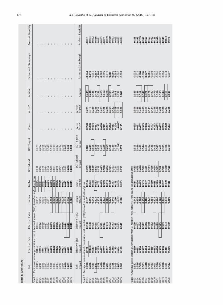
ARTICLE IN PRESS

Tab

le8

.(c

on

tin

ued

)

R.Y. Goyenko et al. / Journal of Financial Economics 92 (2009) 153–181178

ARTICLE IN PRESS

Ta

ble

9A

nn

ua

lsp

rea

dp

rox

ies

com

pa

red

toth

eq

uo

ted

spre

ad

of

the

Do

wp

ort

foli

o1

96

2–

20

00

For

ag

ive

ny

ea

r,th

eb

en

chm

ark

Qu

ote

dsp

rea

d(D

ow

)is

the

pe

rce

nta

ge

qu

ote

dsp

rea

do

fth

eD

ow

Jon

es

Ind

ust

ria

lA

ve

rag

ep

ort

foli

oa

sco

mp

ile

db

yC

ha

rle

sJo

ne

s.Fo

ra

giv

en

ye

ar,

all

spre

ad

pro

xie

sa

re

calc

ula

ted

fro

mC

RS

Pd

ail

yst

ock

pri

cea

nd

vo

lum

ed

ata

for

ea

chst

ock

inth

eD

ow

30

an

dth

en

eq

ua

lly

we

igh

ted

tog

et

the

po

rtfo

lio

va

lue

.Th

esp

rea

dp

rox

ies

are

:R

oll

fro

mR

oll

(19

84

),E

ffe

ctiv

eT

ick

an

dE

ffe

ctiv

e

Tic

k2

de

ve

lop

ed

he

rea

nd

inH

old

en

(20

09

),H

old

en

fro

mH

old

en

(20

09

),G

ibb

sfr

om

Ha

sbro

uck

(20

04

),LO

TM

ixe

d,

Ze

ros,

an

dZ

ero

s2fr

om

Lesm

on

d,

Od

ge

n,

an

dT

rzci

nk

a(1

99

9),

LOT

Y-s

pli

td

ev

elo

pe

dh

ere

,

Am

ihu

dfr

om

Am

ihu

d(2

00

2),

Pa

sto

ra

nd

Sta

mb

au

gh

fro

mP

ast

or

an

dSt

am

ba

ug

h(2

00

3),

an

dth

eA

miv

est

rati

o.

Th

esa

mp

lesi

zeis

39

po

rtfo

lio

-ye

ars

.B

old

nu

mb

ers

are

sta

tist

ica

lly

sig

nifi

can

ta

tth

e5

%le

ve

l.

R.Y. Goyenko et al. / Journal of Financial Economics 92 (2009) 153–181 179

monthly and annually, can usefully estimate high-fre-quency measures, and if so, to determine which measuresare best. Using a sample of 400 randomly selected stocksover the period 1993 to 2005, we compare all priorproxies, three new spread measures, and nine new priceimpact measures. Specifically, we first compute theeffective and realized spreads and several measures ofprice impact from two high-frequency data sets: TAQ andRule 605 data disclosed by market centers to the SEC. Wethen compute the low-frequency measures from dailyreturn and volume data available on CRSP on a monthlyand annual basis. We statistically determine how well thelow-frequency measures capture high-frequency bench-marks.

The evidence is overwhelming that both monthly andannual low-frequency measures capture high-frequencymeasures of transaction costs. Indeed, in many applica-tions the correlations are high and the mean squared errorlow enough that the effort of using high-frequencymeasures is simply not worth the cost. The only realquestion then is: which measure should a researcher use?The answer depends on what, exactly, the researcherwants to measure.

For monthly and annual effective and realized spreads,we find that three measures dominate the remaining ninein correlations and mean squared prediction errors. Thesimplest of the dominant measures is the analytic‘‘Effective Tick.’’ The most computationally intensive isthe ‘‘Holden’’ measure. Intermediate in computationalrequirements is LOT Y-split. All provide statisticallysignificant and useful measures, high correlations, andlow root mean squared errors, regardless of the databasewe use (TAQ or Rule 605). Without considering computa-tional requirements, Holden delivers the best perfor-mance overall. Considering ease of computation,Effective Tick is the best measure to use. Measures widelyused in the literature, namely, Amihud’s Illiquidity, Pastorand Stambaugh’s Gamma, and Amivest’s Liquidity, are notappropriate to use as proxies for effective or realizedspreads.

We find that price impact is more difficult to capture inour data than effective or realized spread. The measuresare not designed to capture the magnitude of high-frequency price impact benchmarks and the correlationswith price impact are lower than in the effective/realizedspread tests. However, both the new class of price impactmeasures we introduce in this paper and the Amihudmeasure do a reasonably good job in the sense that theyproduce statistically significant positive correlations.Pastor and Stambaugh’s Gamma and Amivest’s Liquidityare ineffective in capturing price impact in our data. Wesuggest using either the Amihud measure or using one ofour effective spread measures divided by volume if aresearcher wants to capture price impact.

For specific high-frequency transaction costs bench-marks we suggest different low-frequency measures. Tocapture Lambda (TAQ), which is the coefficient fromregressing return on the square root of signed tradingvolume over five-minute intervals, we suggest eitherAmihud’s Illiquidity or one of the new measures. Tomeasure 5-Minute Price Impact, or the five-minute

ARTICLE IN PRESS

0.0%

0.1%

0.2%

0.3%

0.4%

0.5%

0.6%

0.7%

0.8%

0.9%

1960Year

Dow

por

t. pe

rcen

t quo

ted

spre

ad a

nd s

prea

dpr

oxie

s

Percent quoted spread

LOT Y-split

Holden

Effective Tick

1965 1970 1975 1980 1985 1990 1995 2000

Fig. 1. Dow portfolio percent quoted spread and spread proxies (1962–2000). For a given year, the benchmark is the percent quoted spread of the Dow

Jones Industrial Average portfolio as compiled by Charles Jones. For a given year, all spread proxies are calculated from CRSP daily stock price and volume

data for each stock in the Dow 30 and then equally weighted to get the portfolio value.

R.Y. Goyenko et al. / Journal of Financial Economics 92 (2009) 153–181180

change in midpoint after the trade, we suggest using theAmihud Illiquidity measure.

All price impact measures fail to capture cross-sectional or time-series variation of Static Price Impact(605). It is possible that this difficulty lies primarily in thefact that Rule 605 data exclude block trades, where priceimpact should be most severe. In other words, much of thevariation of Static Price Impact (605) may be noise.However, the new class of price impact measures does agood job in predicting the level of Static Price Impact (605)and has very low mean bias and root mean squared error.

We conduct several robustness checks on theseconclusions. First, we examine the pattern of thesemeasures over time. Second, we examine whether listingexchange matters. Finally, we test the ability of thesemeasures to predict the percent quoted spread of the Dowportfolio from 1962 to 2000. The conclusions are essen-tially the same in these tests. The measures vary over timein their ability to capture high-frequency measures, butthe dominant measures are the same group over time.Interestingly, all measures based on price clustering seemto deteriorate in capturing the effective spread during thedecimals regime, while the Amihud correlations continueto perform reasonably well during the last years of thesample. Further, exchange listing does not matter and thelow-frequency measures do well in predicting the quotedspreads on Dow stocks.

As with any empirical paper several caveats should bementioned. First, using a random sample in this papermeans that caution should be used in applying thesemeasures to other samples or other time periods. Second,we do not know whether the measures are effective on

international data, especially in relation to those stockswith extremely thin trading. Both limitations suggestavenues for future research. With these limitations inmind, we think the results of this paper are strong enoughthat use of the low-frequency proxies to extend assetpricing, market efficiency, and corporate finance researchback in time and around the world is a step that thefinance literature needs to take.

References

Acharya, V., Pedersen, L., 2005. Asset pricing with liquidity risk. Journal

of Financial Economics 77, 375–410.Amihud, Y., 2002. Illiquidity and stock returns: cross-section and time-

series effects. Journal of Financial Markets 5, 31–56.Amihud, Y., Mendelson, H., Lauterbach, B., 1997. Market microstructure

and securities values: evidence from the Tel Aviv stock exchange.

Journal of Financial Economics 45, 365–390.Bekaert, G., Harvey, C., Lundblad, C., 2007. Liquidity and expected

returns: lessons from emerging markets. Review of Financial Studies

20, 1783–1831.Berkman, H., Eleswarapu, V., 1998. Short-term traders and liquidity: a

test using Bombay Stock Exchange data. Journal of Financial

Economics 47, 339–355.Boehmer, E., Jennings, R., Wei, L., 2003. Public disclosure and private

decisions: the case of equity market execution quality. Working

Paper, Indiana University.Cao, C., Field, L., Hanka, G., 2004. Does insider trading impair market

liquidity? Evidence from IPO lockup expirations. Journal of Financial

and Quantitative Analysis 39, 25–46.Chan, L., Jegadeesh, N., Lakonishok, J., 1996. Momentum strategies.

Journal of Finance 51, 1681–1713.Chordia, T., Roll, R., Subrahmanyam, A., 2000. Commonality in liquidity.

Journal of Financial Economics 56, 3–28.Chordia, T., Goyal, A., Sadka, G., Sadka, R., Shivakumar, L., 2008. Liquidity

and the post-earnings-announcement-drift. Working Paper, Univer-

sity of Washington.

ARTICLE IN PRESS

R.Y. Goyenko et al. / Journal of Financial Economics 92 (2009) 153–181 181

Christie, W., Schultz, P., 1994. Why do NASDAQ market makers avoidodd-eighth quotes? Journal of Finance 49, 1813–1840.

Cooper, S., Groth, K., Avera, W., 1985. Liquidity, exchange listing andcommon stock performance. Journal of Economics and Business 37,19–33.

De Bondt, W., Thaler, R., 1985. Does the stock market overreact? Journalof Finance 40, 793–805.

Dennis, P., Strickland, D., 2003. The effect of stock splits on liquidity andexcess returns: evidence from shareholder ownership composition.Journal of Financial Research 26, 355–370.

Fama, E., MacBeth, J., 1973. Risk, return, and equilibrium: empirical tests.Journal of Political Economy 81, 607–636.

Fujimoto, A., 2003. Macroeconomic sources of systematic liquidity.Working Paper, Yale University.

Glosten, L., 1987. Components of the bid–ask spread and the statisticalproperties of transaction prices. Journal of Finance 42, 1293–1307.

Goyenko, R., 2006. Stock and bond pricing with liquidity risk. WorkingPaper, Indiana University.

Harris, L., 1991. Stock price clustering and discreteness. Review ofFinancial Studies 4, 389–415.

Hasbrouck, J., 2004. Liquidity in the futures pits: inferring marketdynamics from incomplete data. Journal of Financial and Quantita-tive Analysis 39, 305–326.

Hasbrouck, J., 2009. Trading costs and returns for US equities: estimatingeffective costs from daily data. Journal of Finance, forthcoming.

Helfin, F., Shaw, K., 2000. Blockholder ownership and market liquidity.Journal of Financial and Quantitative Analysis 35, 621–633.

Holden, C., 2009. New low-frequency liquidity measures. Working Paper,Indiana University.

Huang, R., Stoll, H., 1996. Dealer versus auction markets: a pairedcomparison of execution costs on NASDAQ and the NYSE. Journal ofFinancial Economics 41, 313–357.

Huang, R., Stoll, H., 1997. The components of the bid–ask spread: ageneral approach. Review of Financial Studies 10, 995–1034.

Jegadeesh, N., Titman, S., 1993. Returns to buying winners and sellinglosers: implications for market efficiency. Journal of Finance 48,65–92.

Jegadeesh, N., Titman, S., 2001. Profitability of momentum strategies: anevaluation of alternative explanations. Journal of Finance 56,699–720.

Jones, C., 2002. A century of stock market liquidity and trading costs.Working Paper, Columbia University.

Kalev, P., Pham, P., Steen, A., 2003. Underpricing, stock allocation,ownership structure and post-listing liquidity of newly listed firms.Journal of Banking and Finance 27, 919–947.

Keim, D., Madhavan, A., 1997. Transactions costs and investment style: aninter-exchange analysis of institutional equity trades. Journal ofFinancial Economics 46, 265–292.

Korajczyk, R., Sadka, R., 2008. Pricing the commonality across alternativemeasures of liquidity. Journal of Financial Economics, forthcoming.

Lee, C., Radhakrishna, B., 2000. Inferring investor behavior: evidencefrom TORQ data. Journal of Financial Markets 3, 83–112.

Lee, C., Ready, M., 1991. Inferring trade direction from intraday data.Journal of Finance 46, 733–746.

Lerner, J., Schoar, A., 2004. The illiquidity puzzle: theory and evidencefrom private equity. Journal of Financial Economics 72, 3–40.

Lesmond, D., 2005. Liquidity of emerging markets. Journal of FinancialEonomics 77, 411–452.

Lesmond, D., O’Connor, P, Senbet, L., 2008. Capital structure and equityliquidity. Working Paper, Tulane University.

Lesmond, D., Ogden, J., Trzcinka, C., 1999. A new estimate of transactioncosts. Review of Financial Studies 12, 1113–1141.

Lipson, M., Mortal, S., 2004a. Liquidity and firm characteristics: evidencefrom mergers and acquisitions. Working Paper, University of Georgia.

Lipson, M., Mortal, S., 2004b. Capital structure decision and equitymarket liquidity. Working Paper, University of Georgia.

Pastor, L., Stambaugh, R., 2003. Liquidity risk and expected stock returns.Journal of Political Economy 111, 642–685.

Roll, R., 1984. A simple implicit measure of the effective bid–ask spreadin an efficient market. Journal of Finance 39, 1127–1139.

Rouwenhorst, G., 1998. International momentum strategies. Journal ofFinance 53, 267–284.

Sadka, R., 2006. Liquidity risk and asset pricing. Journal of FinancialEconomics 80, 309–349.

Schrand, C., Verrecchia, R., 2004. Disclosure choice and cost of capital:evidence from underpricing in initial public offerings. WorkingPaper, University of Pennsylvania.

Schultz, P., 2000. Regulatory and legal pressures and the costs of NASDAQtrading. Review of Financial Studies 13, 917–957.

Swinscow, T., 1997. Statistics at Square One, ninth ed. BMJ PublishingGroup, London.

Theil, H., 1966. Applied Economic Forecasts. North-Holland, Amsterdam.Watanabe, A., Watanabe, M., 2006. Time-varying liquidity risk and the

cross section of stock returns. Review of Financial Studies, forthcoming.