Journal of Geodynamics 72 (2013) 1–10

Contents lists available at ScienceDirect

Journal of Geodynamics

journa l homepage: ht tp : / /www.e lsev ier .com/ locate / jog

Observing and understanding the Earth system variations from spacegeodesy

Shuanggen Jina,∗, Tonie van Damb, Shimon Wdowinskic

a Shanghai Astronomical Observatory, Chinese Academy of Sciences, Shanghai 200030, Chinab University of Luxembourg, Luxembourg L-1359, Luxembourgc University of Miami, Miami, FL 33149, USA

a r t i c l e i n f o

Article history:Received 4 July 2013

Received in revised form 5 August 2013

Accepted 6 August 2013

Available online 16 August 2013

Keywords:Space geodesy

Earth system

Interaction

Climate change

a b s t r a c t

The interaction and coupling of the Earth system components that include the atmosphere, hydrosphere,

cryosphere, lithosphere, and other fluids in Earth’s interior, influence the Earth’s shape, gravity field and

its rotation (the three pillars of geodesy). The effects of global climate change, such as sea level rise,

glacier melting, and geoharzards, also affect these observables. However, observations and models of

Earth’s system change have large uncertainties due to the lack of direct high temporal–spatial mea-

surements. Nowadays, space geodetic techniques, particularly GNSS, VLBI, SLR, DORIS, InSAR, satellite

gravimetry and altimetry provide a unique opportunity to monitor and, therefore, understand the pro-

cesses and feedback mechanisms of the Earth system with high resolution and precision. In this paper,

the status of current space geodetic techniques, some recent observations, and interpretations of those

observations in terms of the Earth system are presented. These results include the role of space geo-

detic techniques, atmospheric–ionospheric sounding, ocean monitoring, hydrologic sensing, cryosphere

mapping, crustal deformation and loading displacements, gravity field, geocenter motion, Earth’s oblate-

ness variations, Earth rotation and atmospheric-solid earth coupling, etc. The remaining questions and

challenges regarding observing and understanding the Earth system are discussed.

© 2013 Elsevier Ltd. All rights reserved.

1. Introduction

The Earth system varies continuously due to interactions andcoupling between its main fluid components that include the atmo-sphere, the hydrosphere, the cryosphere, the lithosphere, and theEarth’s interior. Mass redistributions driven by geodynamic pro-cesses in the Earth system affect the Earth’s shape, gravity fieldand rotation. However, the system and components are also beingaffected by global climate change. The Intergovernmental Panel onClimate Change (IPCC) of United Nations reported that the globalclimate has been warming since the middle of the 20th centurydue to increases in atmospheric greenhouse gas concentrations(Pachauri and Reisinger, 2007). To confirm and assess the futureeffects of global warming, still requires additional observations.However, traditional meteorological sensors suffer from a numberof limitations. In addition to being highly labor-intensive to deploy

∗ Corresponding author at: Shanghai Astronomical Observatory, Chinese

Academy of Sciences, Shanghai 200030, China. Tel.: +86 21 34775292;

fax: +86 21 64384618.

E-mail addresses: sgjin@shao.ac.cn, sg.jin@yahoo.com (S. Jin),

tonie.vandam@uni.lu (T. van Dam), shimonw@rsmas.miami.edu (S. Wdowinski).

they also have a low-spatial resolution, e.g., low temporal resolu-tion radiosonde balloons that are launched twice per day (Jin andLuo, 2009; Jin et al., 2009). Another example is ionospheric mon-itoring, in which traditional instruments are very expensive andprovide only low spatial sampling. Furthermore, ionosondes can-not measure the topside ionosphere and sometimes suffer fromabsorption during storms, whereas Incoherent Scatter Radar (ISR)has geographical limitations, and even low-Earth-orbiting satellite(altitudes of 400–800 km) observations cannot provide informationon the whole ionosphere (Jin et al., 2006).

Oceans have been observed by drifting buoys and tide gauges(TG) for almost two centuries (Barnett, 1984). Mean sea level risewas observed using TG through the 20th century. Sea-level risewas thought to be driven by a steric component due to the thermalexpansion of the oceans and a non-steric component due to freshwater input from the melting of continental ice sheets and glaciers(Holgate and Woodworth, 2004; Church and White, 2006; Fenget al., 2013), that affect our living environments, marine ecosys-tems, coasts and marshes. However, TG provides the relative sealevel variations with respect to the land. Furthermore, TG dataare point measurements and are provided at low spatial resolu-tions. We cannot quantify the steric contribution to the sea levelbudget due to the lack of global ocean temperature and salinity

0264-3707/$ – see front matter © 2013 Elsevier Ltd. All rights reserved.http://dx.doi.org/10.1016/j.jog.2013.08.001

2 S. Jin et al. / Journal of Geodynamics 72 (2013) 1–10

observations. In addition, detailed ocean circulation and theexchange between land and ocean water on a global scale are dif-ficult to measure using traditional instruments.

The solid-Earth’s surface and interior are changing constantlybecause of mantle convection, tectonics, and surface processes.These activities cause displacements and deformations of theEarth’s surface, landslides and subsidence, mud-rock flow, andother phenomena. In the past, plate motion was inferred frommarine magnetic anomalies located on both sides of the mid-oceanridges and from the azimuth of transform-faults (at time scalesof millions of years), as well as from historic earthquake sourceparameters. Another issue is that it is difficult to monitor present-day intraplate crustal deformations in sufficient details (Jin and Zhu,2002). For example, current deformation in East Asia is distributedover a broad area extending from Tibet in the south to the Kuril-Japan trench in the east with some micro-plates, such as SouthChina and possibly the Amurian plate, embedded in the deform-ing zone (Jin et al., 2007). Because of the sparse seismicity in theregion and the lack of clear geographical boundaries in the broadplate deformation zones, it has been difficult to describe accuratelythe tectonic kinematics and plate boundaries acting here. Earth-quakes and volcanoes frequently occur worldwide, with notablecases including: the Mw = 9.1 Sumatra Earthquake in 2004; theMw = 8.1 Wenchuan Earthquake in 2008; the Mw = 8.0 Chile Earth-quake in 2010; and the Mw = 9.0 Tohoku Earthquake in 2011. Theseearthquakes took thousands of lives and generated huge tsunamis.Seismometers around the globe can estimate the nature of earth-quakes, but the details of rapid rupture are usually obscured by thelack of near-field near-real-time observations. In addition, observ-ing and modeling Earth’s interior activities are still challenging dueto the complex mass transport and other physical processes actingwithin the Earth system (Jin et al., 2010a; Jin and Feng, 2013).

Therefore, it is hard to observe and model Earth system and envi-ronment changes. Today, Earth observations from space provide aunique opportunity to monitor variations in the various compo-nents of the Earth system. Observations include data from the densedistribution of ground global positioning system (GPS) stations;high resolution space-borne GPS radio occultation; long-term VeryLong Baseline Interferometry (VLBI); Satellite Laser Ranging (SLR);Doppler Orbitography and Radiopositioning Integrated by Satellite(DORIS); Interferometric Synthetic Aperture Radar (InSAR); LightDetection and Ranging (LiDAR); satellite radar and laser altime-try (Abshire et al., 2005); and satellite gravimetry (particularlyCHAMP/GRACE/GOCE) (e.g., Tapley et al., 2004). These observa-tions allow us to measure and monitor small displacements of theEarth’s surface and mass transport with high precision and highspatial–temporal resolutions. These data provide a unique oppor-tunity to investigate mass transport associated with geodynamics,natural hazards, and climate change and to better understand theprocesses themselves and their interactions within the Earth sys-tem. In this paper, the different space geodetic techniques and Earthsystem interactions are introduced. Recent observations and mod-eling results from space geodesy that allow us to infer changes inthe atmosphere, oceans, hydrosphere, cryosphere, lithosphere, andthe Earth’s deep interior are presented.

2. Space geodetic techniques and observations

The word “geodesy” etymologically comes from the Greek“geôdaisia”: “dividing the Earth”. Today, geodesy is defined asmeasuring the Earth’s size, shape, orientation, gravitational fieldand their variations with time using geodetic techniques, e.g.,Arc measurements (historic), Triangulation, Trilateration, Travers-ing, Leveling, Zenith or vertical angles measurement and groundgravimetry. However, these traditional geodetic techniques are

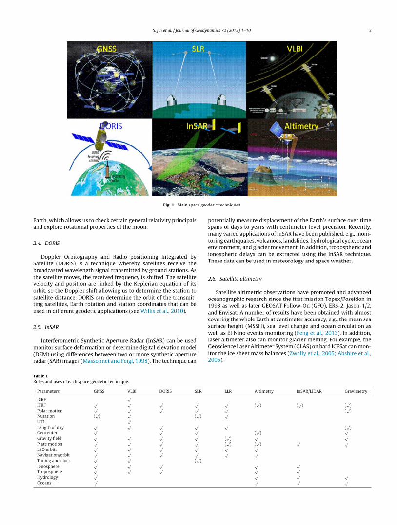
labor intensive. The advent of space geodesy has represented arevolution for the space age and Earth exploration, e.g., VLBI, SLR,DORIS, GNSS, InSAR/LiDAR, and satellite radar and laser altimetry(see Fig. 1). These space geodetic techniques are capable of mea-suring and precisely monitoring small changes of the parametersthey observe with high spatial–temporal resolution. The differentroles and uses of each space geodetic technique are summarizedin Table 1. In the following discussion, the main space geodetictechniques are briefly introduced.

2.1. GNSS

Global Navigation Satellite System (GNSS) is a recent term usedto describe the various satellite navigation systems, such as GPS,GLONASS, Beidou and Galileo. The Global Positioning System (GPS)with its unprecedented precision, has provided great contributionsto navigation, positioning, timing and scientific questions relatedto precise positioning on Earth’s surface, since it became fullyoperational in 1994 (Jin et al., 2011a). Today, a number of Earthsystem science questions have been successfully investigated,including the establishment of a high precision International Ter-restrial Reference Frame (ITRF), Earth rotation, geocenter motion,time-variability of the gravity field, orbit determination as well asremote sensing of the atmosphere, hydrology and oceans. Withthe development of the next generation of multi-frequency andmulti-system GNSS constellations, including the U.S.’s modernizedGPS-IIF and planned GPS-III, Russia’s restored GLONASS, the comingEuropean Union’s GALILEO system, and China’s Beidou/COMPASSsystem, as well as a number of regional systems including Japan’sQuasi-Zenith Satellite System (QZSS) and India’s Regional Naviga-tion Satellite Systems (IRNSS), more applications and opportunitieswill be realized to explore the Earth system using ground and spaceborne GNSS.

2.2. VLBI

Very-long-baseline interferometry, VLBI, plays a key role inspace geodesy by receiving natural quasars signals at two ormore Earth-based radio telescopes. VLBI is particularly impor-tant in establishing the International Celestial Reference Frame(ICRF). With the global VLBI tracking network, VLBI can be usedto monitor plate motion, crustal deformation, polar motion andlength-of-day as well as being used for deep space exploration.The “VLBI2010: Current and Future Requirements for GeodeticVLBI Systems” provided a path to a next-generation system withunprecedented new capabilities and accuracies, including 1 mmposition and 0.1 mm/year velocity measurement accuracy, con-tinuous observations for station positions and Earth orientationparameters. Additional applications will be developed in the nearfuture (Titov, 2010). For example, the Chinese VLBI Network (CVN)has been upgraded (e.g., two VLBI radio telescopes in Shanghaiand Urumqi, and several proposed new VLBI2010-type system) andnew applications such as successfully tracking the China’s Chang’E-1/2 lunar exploration probes (Wei et al., 2013).

2.3. SLR/LLR

Satellite Laser Ranging (SLR) systems precisely determine thedistance of the satellites above the Earth’s geocenter by measuringthe time to send and receive short laser pulses. These data havebeen widely used in precise orbit determination (POD) of artificialsatellites and station motions. In addition, since the low-earth-orbit(LEO) laser ranging satellites are sensitive to the low-degree gravityfield, SLR is considered the gold-standard in monitoring geocenterand C20 (Cheng and Tapley, 2004; Jin et al., 2011b). Lunar LaserRanging (LLR) can measure the distance between the moon and

S. Jin et al. / Journal of Geodynamics 72 (2013) 1–10 3

Fig. 1. Main space geodetic techniques.

Earth, which allows us to check certain general relativity principalsand explore rotational properties of the moon.

2.4. DORIS

Doppler Orbitography and Radio positioning Integrated bySatellite (DORIS) is a technique whereby satellites receive thebroadcasted wavelength signal transmitted by ground stations. Asthe satellite moves, the received frequency is shifted. The satellitevelocity and position are linked by the Keplerian equation of itsorbit, so the Doppler shift allowing us to determine the station tosatellite distance. DORIS can determine the orbit of the transmit-ting satellites, Earth rotation and station coordinates that can beused in different geodetic applications (see Willis et al., 2010).

2.5. InSAR

Interferometric Synthetic Aperture Radar (InSAR) can be usedmonitor surface deformation or determine digital elevation model(DEM) using differences between two or more synthetic apertureradar (SAR) images (Massonnet and Feigl, 1998). The technique can

potentially measure displacement of the Earth’s surface over timespans of days to years with centimeter level precision. Recently,many varied applications of InSAR have been published, e.g., moni-toring earthquakes, volcanoes, landslides, hydrological cycle, oceanenvironment, and glacier movement. In addition, tropospheric andionospheric delays can be extracted using the InSAR technique.These data can be used in meteorology and space weather.

2.6. Satellite altimetry

Satellite altimetric observations have promoted and advancedoceanographic research since the first mission Topex/Poseidon in1993 as well as later GEOSAT Follow-On (GFO), ERS-2, Jason-1/2,and Envisat. A number of results have been obtained with almostcovering the whole Earth at centimeter accuracy, e.g., the mean seasurface height (MSSH), sea level change and ocean circulation aswell as El Nino events monitoring (Feng et al., 2013). In addition,laser altimeter also can monitor glacier melting. For example, theGeoscience Laser Altimeter System (GLAS) on bard ICESat can mon-itor the ice sheet mass balances (Zwally et al., 2005; Abshire et al.,2005).

Table 1

Roles and uses of each space geodetic technique.

Parameters GNSS VLBI DORIS SLR LLR Altimetry InSAR/LiDAR Gravimetry

ICRF√

ITRF√ √ √ √ √

(√

) (√

) (√

)

Polar motion√ √ √ √ √

(√

)

Nutation (√

)√

(√

)√

UT1√

Length of day√ √ √ √ √

(√

)

Geocenter√ √ √

(√

)√

Gravity field√ √ √ √

(√

)√ √

Plate motion√ √ √ √

(√

) (√

)√ √

LEO orbits√ √ √ √ √ √

Navigation/orbit√ √ √ √ √ √

Timing and clock√ √

(√

)

Ionosphere√ √ √ √ √

Troposphere√ √ √ √ √

Hydrology√ √ √ √

Oceans√ √ √ √

4 S. Jin et al. / Journal of Geodynamics 72 (2013) 1–10

Fig. 2. Earth system components and interaction.

2.7. Satellite gravimetry

With the recent development of the low-earth orbit (LEO)satellite gravimetry, the precision and temporal resolution of theEarth’s gravity field model has been greatly improved. Satellitegravimetry is a successful innovation and breakthrough in thefield of geodesy, following the Global Positioning System (GPS).Unlike the traditional terrestrial gravity measurements, the mostadvanced SST (Satellite-to-Satellite Tracking) and SGG (SatelliteGravity Gradiometry) techniques are used to estimate the globalhigh-precision gravity field and its variations (Knudsen et al.,2011). Satellite-to-Satellite Tracking technique includes the so-called high–low satellite-to-satellite tracking (hl-SST) and low–lowsatellite-to-satellite tracking (ll-SST) (Wolff, 1969), which can pre-cisely determine the variation rate of the distance between twosatellites. Satellite gravimetry, particularly recent Gravity Recoveryand Climate Experiment (GRACE), can monitor the mass transportand redistribution in the Earth system, which has been widelyapplied in geodesy, oceanography, hydrology, ice mass change, geo-dynamics and geophysics (Wahr et al., 1998; Tapley et al., 2004;Famiglietti et al., 2011; Jin and Feng, 2013).

3. Space geodesy and earth system interaction

The Earth system is very complex due to the interaction andcoupling of its components (Fig. 2). For example, melting conti-nental glaciers will result in rising sea levels, tectonic activities andreservoir accumulated water may lead to hazards, e.g., earthquakes,tsunamis, landslides and mud-rock flows and the atmosphericpressure loading will change the shape, geocenter, oblateness androtation of the Earth, etc.

Today space geodetic techniques with high precision andtemporal–spatial resolution can measure and monitor suchchanges within the Earth system, including Earth rotation,Earth’s oblateness, geocenter, geometry and deformation, grav-ity field, atmosphere, oceans, hydrosphere, cryosphere, crust,ocean/atmospheric/polar tides, ocean/atmospheric/hydrologicalloading, tectonic motions, volcanoes, earthquakes, tsunamis,glacier istostatic adjustment (GIA) and landslides, etc. Fig. 3 showsthe role of space geodesy in observing and understanding the Earthsystem. The reference frame is a benchmark for Earth rotation,geometry and deformation and gravity field measurements that canbe precisely determined using space geodesy. Earth system changes

Space Techniques

GNSS

VLBI

DORIS

SLR/LLR

InSAR

LiDAR

Altimetry

Satellite Gravimetry

…

Terrestrial Techniques

Leveling

Tide Gauge

Gravimetry

Tiangulation

…

Earth System

Atmosphere Oceans

HydrosphereCryosphere

Crust MantleCore …

Tides Loadings

Geocenter motionsTectonic motions

VolcanoesEarthquakes

Tsunamis GIA

Landslides….

Geometry & Deformation

Gravity Field

ReferenceFrame

Earth

Rotation

Fig. 3. Space geodesy and earth system interaction.

affect the Earth’s rotation, geometry and deformation and gravityfield as well as reference frame.

4. Observing and understanding Earth system

4.1. Atmospheric sounding

Space techniques’ radio signals propagate through the Earth’sneutral atmosphere and ionosphere. This results in lengtheningthe geometric path of the ray, usually referred to as the “tro-pospheric delay and ionospheric delay.” These delays are one ofmajor error sources for space techniques. Today, the space tech-niques such as GPS, VLBI, InSAR, DORIS and altimetry are able tomeasure such delays and corresponding precipitable water vapor(PWV) and ionospheric total electron content (TEC) with a highresolution and precision. These products have been widely appliedin meteorology, climatology, numerical weather models, atmo-spheric science and space weather (e.g., Jin et al., 2006; Jin andPark, 2007; Jin et al., 2008, 2009; Jin and Luo, 2009). For example,Fig. 4 shows the long-term vertical TEC variations from GPS at the

2002 2003 2004 2005 2006 2007 2008 2009 2010 2011 2012 20130

10

20

30

40

50

VT

EC

(T

EC

U)

VTEC at (Lat: -87.5o; Lon: 120

o)

Time (year)

2002 2003 2004 2005 2006 2007 2008 2009 2010 2011 2012 20130

100

200

300

Flu

x (1

0-2

2 W

M-2

Hz-1

)

Time (year)

10.7 cm Solar Flux

Fig. 4. Vertical TEC (VTEC) time series at (120 E◦ , −87.5 S◦) and 10.7 cm Solar Flux.

S. Jin et al. / Journal of Geodynamics 72 (2013) 1–10 5

point (120 E◦, −87.5 S◦), which are mainly affected by solar activity.Additionally, the space-borne GPS radio occultation (RO) missionscan estimate atmospheric and ionospheric products, including thepressure, temperature, water vapor, total electron content (TEC)and electron density as well as their variation characteristics, e.g.,the US/Argentina SAC-C, German CHAMP (CHAllenging Minisatel-lite Payload), US/Germany GRACE (Gravity Recovery and ClimateExperiment), Taiwan/US FORMOSAT-3/COSMIC (FORMOsa SATel-lite mission – 3/Constellation Observing System for Meteorology,Ionosphere and Climate) satellites, the German TerraSAR-X satel-lites and the European MetOp (Schmidt et al., 2010; Jin et al., 2011a).

4.2. Ocean monitoring

The oceans have been well monitored by satellite altimetry forabout two decades. These data provide information on the meansea surface height (MSSH), ocean circulation, tides and sea levelchange. The sea level change includes the steric and non-steric seachanges. While the steric sea level change, i.e., thermal expansion,is well estimated by Argo observations, the non-steric component,i.e., eustatic sea level change, related to mass changes driven by theaddition of water to the oceans from the melting of continental icesheets and fresh water in rivers and lakes (Feng et al., 2013) is moredifficult to estimate. The difficulty is due to the highly uncertainestimates of the Antarctic and Greenland mass and land reservoirs.The satellite-based GRACE observations provide a unique oppor-tunity to directly measure the global ocean and continental watermass change. For example, Fig. 5 shows the sea level change incm/year from satellite altimetry, Argo and GRACE (2002–2011),which generally quantify the total sea level change budget.

In addition, GNSS-Reflectometry (GNSS-R) is a new innova-tive and promising approach in ocean remote sensing. In addition,the technique poses many potential advantages (Jin et al., 2011a),including primarily global coverage and long-term satellite missionlifetime. In the last few years, several experiments were undertakenand numerous advancements were realized. The first GPS signalsreflected from the sea surface inside tropical cyclones were ana-lyzed, and the wind speed results were obtained (Katzberg et al.,2001). Currently, the GPS reflected signals from the ocean sur-face can measure sea surface height with the achievable accuracy(Martin-Neira et al., 2001; Katzberg and Dunion, 2009).

4.3. Hydrologic sensing

The power level of the GPS reflected signal from the landcontains information about the soil moisture, dielectric constant,surface roughness, and possible vegetative cover of the reflect-ing surface. Katzberg et al. (2006) obtained the soil reflectivityand dielectric constant using a GPS reflectometer installed on anHC130 aircraft during the Soil Moisture Experiment 2002 (SMEX02)near Ames, Iowa, which were consistent with results found forother microwave techniques operating at L-band. In addition,the multi-path from ground GPS networks is possibly related tothe near-surface soil moisture. Larson et al. (2008) found nearlyconsistent fluctuations in near-surface soil moisture from theground-based observations of GPS multi-path. They found GPS esti-mates of soil moisture were comparable to estimates in the top 5 cmof soil measured from conventional sensors.

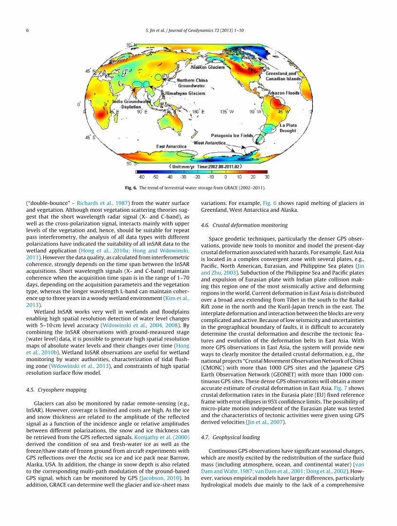
Satellite gravimetry, in particular GRACE, can determine themonthly terrestrial water storage change. Fig. 6 shows the trend ofterrestrial water storage change in the world based on GRACE data(August 2002–February 2011), which reflect groundwater deple-tion, drought and floods. For example, the terrestrial water storageis falling by about −15.5 mm/year in the northwest region of Indiadue to groundwater depletion (Rodell et al., 2009). The Amazonbasin in South American has increased rates of terrestrial water

Fig. 5. Sea level change in cm/year from satellite altimetry, Argo and GRACE

(2002–2011).

storage reserves with about 20.5 mm/year due to recent floods. Inthe La Plata region of South America, the terrestrial water storageis falling at a rate of −9.8 mm/year due to recent droughts.

4.4. Wetland mentoring by InSAR

Wetland InSAR is a unique application of the InSAR technique,because unlike all other applications that detect displacements ofsolid surfaces, wetland InSAR detects changes of aquatic surfaces.The method works, because the radar pulse is backscattered twice

6 S. Jin et al. / Journal of Geodynamics 72 (2013) 1–10

Fig. 6. The trend of terrestrial water storage from GRACE (2002–2011).

(“double-bounce” – Richards et al., 1987) from the water surfaceand vegetation. Although most vegetation scattering theories sug-gest that the short wavelength radar signal (X- and C-band), aswell as the cross-polarization signal, interacts mainly with upperlevels of the vegetation and, hence, should be suitable for repeatpass interferometry, the analysis of all data types with differentpolarizations have indicated the suitability of all inSAR data to thewetland application (Hong et al., 2010a; Hong and Wdowinski,2011). However the data quality, as calculated from interferometriccoherence, strongly depends on the time span between the InSARacquisitions. Short wavelength signals (X- and C-band) maintaincoherence when the acquisition time span is in the range of 1–70days, depending on the acquisition parameters and the vegetationtype, whereas the longer wavelength L-band can maintain coher-ence up to three years in a woody wetland environment (Kim et al.,2013).

Wetland InSAR works very well in wetlands and floodplainsenabling high spatial resolution detection of water level changeswith 5–10 cm level accuracy (Wdowinski et al., 2004, 2008). Bycombining the InSAR observations with ground-measured stage(water level) data, it is possible to generate high spatial resolutionmaps of absolute water levels and their changes over time (Honget al., 2010b). Wetland InSAR observations are useful for wetlandmonitoring by water authorities, characterization of tidal flush-ing zone (Wdowinski et al., 2013), and constraints of high spatialresolution surface flow model.

4.5. Cryosphere mapping

Glaciers can also be monitored by radar remote-sensing (e.g.,InSAR). However, coverage is limited and costs are high. As the iceand snow thickness are related to the amplitude of the reflectedsignal as a function of the incidence angle or relative amplitudesbetween different polarizations, the snow and ice thickness canbe retrieved from the GPS reflected signals. Komjathy et al. (2000)derived the condition of sea and fresh-water ice as well as thefreeze/thaw state of frozen ground from aircraft experiments withGPS reflections over the Arctic sea ice and ice pack near Barrow,Alaska, USA. In addition, the change in snow depth is also relatedto the corresponding multi-path modulation of the ground-basedGPS signal, which can be monitored by GPS (Jacobson, 2010). Inaddition, GRACE can determine well the glacier and ice-sheet mass

variations. For example, Fig. 6 shows rapid melting of glaciers inGreenland, West Antarctica and Alaska.

4.6. Crustal deformation monitoring

Space geodetic techniques, particularly the denser GPS obser-vations, provide new tools to monitor and model the present-daycrustal deformation associated with hazards. For example, East Asiais located in a complex convergent zone with several plates, e.g.,Pacific, North American, Eurasian, and Philippine Sea plates (Jinand Zhu, 2003). Subduction of the Philippine Sea and Pacific platesand expulsion of Eurasian plate with Indian plate collision mak-ing this region one of the most seismically active and deformingregions in the world. Current deformation in East Asia is distributedover a broad area extending from Tibet in the south to the BaikalRift zone in the north and the Kuril-Japan trench in the east. Theinterplate deformation and interaction between the blocks are verycomplicated and active. Because of low seismicity and uncertaintiesin the geographical boundary of faults, it is difficult to accuratelydetermine the crustal deformation and describe the tectonic fea-tures and evolution of the deformation belts in East Asia. Withmore GPS observations in East Asia, the system will provide newways to clearly monitor the detailed crustal deformation, e.g., thenational projects “Crustal Movement Observation Network of China(CMONC) with more than 1000 GPS sites and the Japanese GPSEarth Observation Network (GEONET) with more than 1000 con-tinuous GPS sites. These dense GPS observations will obtain a moreaccurate estimate of crustal deformation in East Asia. Fig. 7 showscrustal deformation rates in the Eurasia plate (EU) fixed referenceframe with error ellipses in 95% confidence limits. The possibility ofmicro-plate motion independent of the Eurasian plate was testedand the characteristics of tectonic activities were given using GPSderived velocities (Jin et al., 2007).

4.7. Geophysical loading

Continuous GPS observations have significant seasonal changes,which are mostly excited by the redistribution of the surface fluidmass (including atmosphere, ocean, and continental water) (vanDam and Wahr, 1987; van Dam et al., 2001; Dong et al., 2002). How-ever, various empirical models have larger differences, particularlyhydrological models due mainly to the lack of a comprehensive

S. Jin et al. / Journal of Geodynamics 72 (2013) 1–10 7

Fig. 7. Crustal deformation rates in the Eurasia plate (EU) fixed reference frame with

error ellipses in 95% confidence limits.

global network for routine monitoring of the appropriate hydrolog-ical parameters. The satellite mission, GRACE, has provided globalsurface fluid mass transport for more than a decade. The verticalloading displacements from GPS, GRACE and geophysical modelsare computed and compared, and at most global sites, the root meansquare (RMS) of GPS coordinate time series is reduced after remov-ing the GRACE and models estimates, and the annual variations ofthe GPS height at most sites agree well with GRACE estimates inthe amplitude and phase (Fig. 8) (Zhang et al., 2012). For example,Fig. 9 shows the vertical displacement time series from GPS, GRACEand geophysical models at BRAZ site. It indicates that the nonlinearseasonal GPS vertical displacement variations are mainly causedby the geophysical loading effects. However, at some sites, partic-ularly in the Antarctica, some ocean coasts, small peninsulas andEurope, discrepancy has been found between the GPS and GRACEestimates (e.g., van Dam et al., 2007). The remaining disagreementmay be due to the GPS technical errors and GRACE accuracy (e.g.,

2002 2003 2004 2005 2006 2007 2008 2009-20

-15

-10

-5

0

5

10

15

20

25

Time(year)

Ver

tical

dis

plac

emen

t re

sidu

als(

mm

)

BRAZ

GPS

GRACE

MODEL

Fig. 9. Monthly vertical displacement time series from GPS, GRACE and geophysical

models at BRAZ site.

Jin et al., 2005). It needs to be further investigated using longer andmore GPS and GRACE measurements.

4.8. Geocenter and Earth’s oblateness variations

The transfer and redistribution of the Earth’s atmosphere,ocean and land water masses due to the tectonic activities andglobal climate change can lead to variations of Earth’s oblate-ness (J2) and geocenter motion (Jin et al., 2010a, 2011b). Satellitelaser ranging (SLR) can well estimate the geocenter motion anddegree-2 zonal gravitational coefficient variations, but subjectingto sparse and unevenly distributed SLR stations as well as higher-altitude laser satellites. Although the new generation of satellitegravity GRACE has largely improved the lower-order coefficientestimates with orders of magnitude, but is not sensitive to geo-center and J2. Nowadays, continuous GPS observations can providehigh precision 3-dimensional coordinate time series, which can

GRACE 10 mm

GPS 10 mm

MODEL 10 mm

180

o W

120

o W

60o W

0o

60 oE

120 oE

180 oW

80oS

40oS

0o

40oN

80oN

longitude

latit

ude

Fig. 8. Annual variations of vertical displacements from GPS, GRACE and geophysical models.

8 S. Jin et al. / Journal of Geodynamics 72 (2013) 1–10

2003 2004 2005 2006 2007 2008 2009-8

-6

-4

-2

0

2

4

6

8

Time (year)

ΔJ2 (

X10

-10 )

GPS GPS+OBP GPS+OBP+GRACE SLR GRACE Models

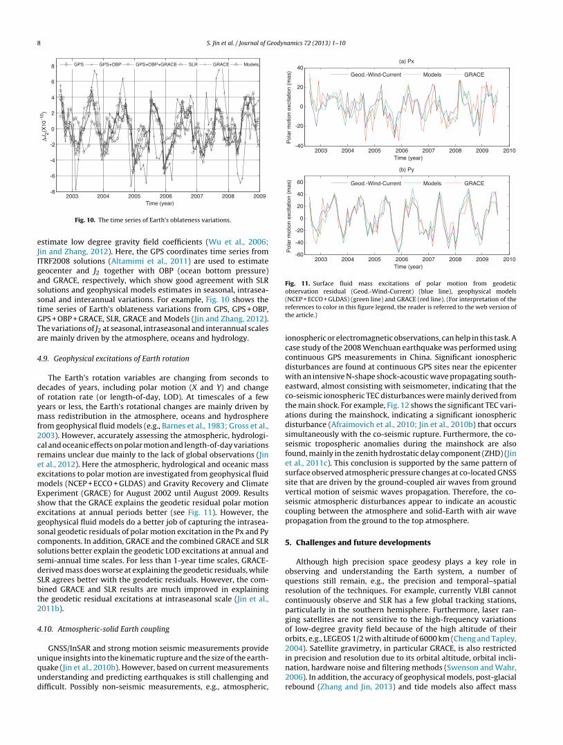
Fig. 10. The time series of Earth’s oblateness variations.

estimate low degree gravity field coefficients (Wu et al., 2006;Jin and Zhang, 2012). Here, the GPS coordinates time series fromITRF2008 solutions (Altamimi et al., 2011) are used to estimategeocenter and J2 together with OBP (ocean bottom pressure)and GRACE, respectively, which show good agreement with SLRsolutions and geophysical models estimates in seasonal, intrasea-sonal and interannual variations. For example, Fig. 10 shows thetime series of Earth’s oblateness variations from GPS, GPS + OBP,GPS + OBP + GRACE, SLR, GRACE and Models (Jin and Zhang, 2012).The variations of J2 at seasonal, intraseasonal and interannual scalesare mainly driven by the atmosphere, oceans and hydrology.

4.9. Geophysical excitations of Earth rotation

The Earth’s rotation variables are changing from seconds todecades of years, including polar motion (X and Y) and changeof rotation rate (or length-of-day, LOD). At timescales of a fewyears or less, the Earth’s rotational changes are mainly driven bymass redistribution in the atmosphere, oceans and hydrospherefrom geophysical fluid models (e.g., Barnes et al., 1983; Gross et al.,2003). However, accurately assessing the atmospheric, hydrologi-cal and oceanic effects on polar motion and length-of-day variationsremains unclear due mainly to the lack of global observations (Jinet al., 2012). Here the atmospheric, hydrological and oceanic massexcitations to polar motion are investigated from geophysical fluidmodels (NCEP + ECCO + GLDAS) and Gravity Recovery and ClimateExperiment (GRACE) for August 2002 until August 2009. Resultsshow that the GRACE explains the geodetic residual polar motionexcitations at annual periods better (see Fig. 11). However, thegeophysical fluid models do a better job of capturing the intrasea-sonal geodetic residuals of polar motion excitation in the Px and Pycomponents. In addition, GRACE and the combined GRACE and SLRsolutions better explain the geodetic LOD excitations at annual andsemi-annual time scales. For less than 1-year time scales, GRACE-derived mass does worse at explaining the geodetic residuals, whileSLR agrees better with the geodetic residuals. However, the com-bined GRACE and SLR results are much improved in explainingthe geodetic residual excitations at intraseasonal scale (Jin et al.,2011b).

4.10. Atmospheric-solid Earth coupling

GNSS/InSAR and strong motion seismic measurements provideunique insights into the kinematic rupture and the size of the earth-quake (Jin et al., 2010b). However, based on current measurementsunderstanding and predicting earthquakes is still challenging anddifficult. Possibly non-seismic measurements, e.g., atmospheric,

2003 2004 2005 2006 2007 2008 2009 2010-40

-20

0

20

40

Time (year)

Pol

ar m

otio

n ex

cita

tion

(mas

)

(a) Px

2003 2004 2005 2006 2007 2008 2009 2010-60

-40

-20

0

20

40

60

Time (year)

Pol

ar m

otio

n ex

cita

tion

(mas

)

(b) Py

Geod.-Wind-Current Models GRACE

Geod.-Wind-Current Models GRACE

Fig. 11. Surface fluid mass excitations of polar motion from geodetic

observation residual (Geod.-Wind-Current) (blue line), geophysical models

(NCEP + ECCO + GLDAS) (green line) and GRACE (red line). (For interpretation of the

references to color in this figure legend, the reader is referred to the web version of

the article.)

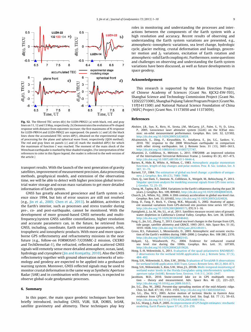
ionospheric or electromagnetic observations, can help in this task. Acase study of the 2008 Wenchuan earthquake was performed usingcontinuous GPS measurements in China. Significant ionosphericdisturbances are found at continuous GPS sites near the epicenterwith an intensive N-shape shock-acoustic wave propagating south-eastward, almost consisting with seismometer, indicating that theco-seismic ionospheric TEC disturbances were mainly derived fromthe main shock. For example, Fig. 12 shows the significant TEC vari-ations during the mainshock, indicating a significant ionosphericdisturbance (Afraimovich et al., 2010; Jin et al., 2010b) that occurssimultaneously with the co-seismic rupture. Furthermore, the co-seismic tropospheric anomalies during the mainshock are alsofound, mainly in the zenith hydrostatic delay component (ZHD) (Jinet al., 2011c). This conclusion is supported by the same pattern ofsurface observed atmospheric pressure changes at co-located GNSSsite that are driven by the ground-coupled air waves from groundvertical motion of seismic waves propagation. Therefore, the co-seismic atmospheric disturbances appear to indicate an acousticcoupling between the atmosphere and solid-Earth with air wavepropagation from the ground to the top atmosphere.

5. Challenges and future developments

Although high precision space geodesy plays a key role inobserving and understanding the Earth system, a number ofquestions still remain, e.g., the precision and temporal–spatialresolution of the techniques. For example, currently VLBI cannotcontinuously observe and SLR has a few global tracking stations,particularly in the southern hemisphere. Furthermore, laser ran-ging satellites are not sensitive to the high-frequency variationsof low-degree gravity field because of the high altitude of theirorbits, e.g., LEGEOS 1/2 with altitude of 6000 km (Cheng and Tapley,2004). Satellite gravimetry, in particular GRACE, is also restrictedin precision and resolution due to its orbital altitude, orbital incli-nation, hardware noise and filtering methods (Swenson and Wahr,2006). In addition, the accuracy of geophysical models, post-glacialrebound (Zhang and Jin, 2013) and tide models also affect mass

S. Jin et al. / Journal of Geodynamics 72 (2013) 1–10 9

Fig. 12. The filtered TEC series dI(t) for LUZH-PRN22 (a) with black, red, and gray

lines on 11, 12 and 13 May, respectively. (b) Demonstrates the evolution of N-shaped

response with distance from epicenter increase; the first maximums of N-response

for LUZH-PRN14 and LUZH-PRN22 are superposed. On panels (c) and (d) the black

lines show the accumulated TEC series dIP(t), obtained on the experimental stage

of processing for the plane and spherical wave front, respectively (QOA method).

The red and gray lines on panels (c) and (d) mark the modeled dIP(t) for which

the maximum of function C was reached. The moment of the main shock of the

Wenchuan earthquake is marked by blue shaded triangles. (For interpretation of the

references to color in this figure legend, the reader is referred to the web version of

the article.)

transport results. With the launch of the next generation of gravitysatellites, improvement of measurement precision, data processingmethods, geophysical models, and extension of the observationtime, we will be able to detect with higher precision global terres-trial water storage and ocean mass variations to get more detailedinformation of Earth system.

GNSS has greatly advanced geoscience and Earth system sci-ence since 1994, but lots of error sources are still not resolved(e.g., Jin et al., 2005; Chen et al., 2013). In addition, activities inthe Earth’s interior, such as processes and stress transfer duringpre-, co- and post-earthquake, cannot be monitored. With thedevelopment of more ground-based GNSS networks and multi-frequency/system GNSS satellite constellations, higher resolutionand accurate parameters can, in the future, be retrieved fromGNSS, including, coordinate, Earth orientation parameters, orbit,tropspheric and ionospheric products. With more and more space-borne GPS reflectometry and refractometry missions in the nearfuture (e.g., follow-on FORMOSAT-7/COSMIC-2 mission, CICEROand TechDemoSat-1), the refracted, reflected and scattered GNSSsignals will remotely sense more detailed atmosphere, ocean, land,hydrology and cryosphere (Jin and Komjathy, 2010). Also the GNSSreflectometry together with ground observation networks of seis-mology and geodesy are expected to be applied into a geohazardwarning system. Moreover, GNSS reflected signals may be used tomonitor crustal deformation in the same way as Synthetic ApertureRadar (SAR) and in combination with other sensors, is expected toobserve global-scale geodynamic processes.

6. Summary

In this paper, the main space geodetic techniques have beenbriefly introduced, including GNSS, VLBI, SLR, DORIS, InSAR,satellite gravimetry and altimetry. These techniques play key

roles in monitoring and understanding the processes and inter-actions between the components of the Earth system with ahigh resolution and accuracy. Recent results of observing andunderstanding the Earth system variations are presented, e.g.,atmospheric–ionospheric variations, sea level change, hydrologiccycle, glacier melting, crustal deformation and loadings, geocen-ter motion and J2 variations, excitation of Earth rotation andatmospheric-solid Earth coupling etc. Furthermore, some questionsand challenges on observing and understanding the Earth systemvariations have been discussed, as well as future developments inspace geodesy.

Acknowledgement

This research is supported by the Main Direction Projectof Chinese Academy of Sciences (Grant No. KJCX2-EW-T03),Shanghai Science and Technology Commission Project (Grant No.12DZ2273300), Shanghai Pujiang Talent Program Project (Grant No.11PJ1411500) and National Natural Science Foundation of China(NSFC) Project (Grant Nos. 11173050 and 11373059).

References

Abshire, J.B., Sun, X., Riris, H., Sirota, J.M., McGarry, J.F., Palm, S., Yi, D., Liiva,P., 2005. Geoscience laser altimeter system (GLAS) on the ICESat mis-sion: on-orbit measurement performance. Geophys. Res. Lett. 32, L21S02,http://dx.doi.org/10.1029/2005GL024028.

Afraimovich, E., Ding, F., Kiryushkin, V., Astafyeva, E., Jin, S.G., Sankov, V.,2010. TEC response to the 2008 Wenchuan earthquake in comparisonwith other strong earthquakes. Int. J. Remote Sens. 31 (13), 3601–3613,http://dx.doi.org/10.1080/01431161003727747.

Altamimi, Z., Collilieux, X., Métivier, L., 2011. ITRF2008: an improved solutionof the International Terrestrial Reference Frame. J. Geodesy 85 (8), 457–473,http://dx.doi.org/10.1007/s00190-011-0444-4.

Barnes, R., Hide, R., White, A., Wilson, C., 1983. Atmospheric angular momentumfunctions, length of day changes and polar motion. Proc. R. Soc. London, Ser. A387, 31–73.

Barnett, T.P., 1984. The estimation of global sea level change: a problem of unique-ness. J. Geophys. Res. 89 (C5), 7980–7988.

Chen, Q., van Dam, T., Sneeuw, N., Collilieux, X., Weigelt, M., Rebischung, P., 2013.Singular spectrum analysis for modeling seasonal signals from GPS time series.J. Geodyn. 72, 25–35.

Cheng, M., Tapley, B.D., 2004. Variations in the Earth’s oblateness during the past 28years. J. Geophys. Res. 109, B09402, http://dx.doi.org/10.1029/2004JB003028.

Church, J.A., White, N.J., 2006. A 20th century acceleration in global sea-level rise.Geophys. Res. Lett. 33, L01602, http://dx.doi.org/10.1029/2005GL024826.

Dong, D., Fang, P., Bock, Y., Cheng, M.K., Miyazaki, S., 2002. Anatomy of appar-ent seasonal variations from GPS-derived site position time series 107 (B4),http://dx.doi.org/10.1029/2001JB000573, ETG 9 1–16.

Famiglietti, J., Lo, M., Ho, S.L., et al., 2011. Satellites measure recent rates of ground-water depletion in California’s Central Valley. Geophys. Res. Lett. 38, L03403,http://dx.doi.org/10.1029/2010GL046442.

Feng, G., Jin, S.G., Zhang, T., 2013. Coastal sea level changes in the Europe from GPS,tide gauge, satellite altimetry and GRACE, 1993–2011. Adv. Space Res. 51 (6),1019–1028, http://dx.doi.org/10.1016/j.asr.2012.09.011.

Gross, R.S., Fukumori, I., Menemenlis, D., 2003. Atmospheric and oceanic excita-tion of the Earth’s wobbles during 1980–2000. J. Geophys. Res. 108 (B8), 2370,http://dx.doi.org/10.1029/2002JB002143.

Holgate, S.J., Woodworth, P.L., 2004. Evidence for enhanced coastalsea level rise during the 1990s. Geophys. Res. Lett. 31, L07305,http://dx.doi.org/10.1029/2004GL019626.

Hong, S.-H, Wdowinski, S., 2011. Evaluation of the quad-polarimetric RADARSAT-2 observations for the wetland InSAR application. Can. J. Remote Sens. 37 (5),484–492.

Hong, S.H., Wdowinski, S., Kim, S.W., 2010a. Evaluation of TerraSAR-X observationsfor wetland InSAR application. IEEE Trans. Geosci. Remote Sens. 48 (2), 864–873.

Hong, S.H., Wdowinski, S., Kim, S.W., Won, J.S., 2010b. Multi-temporal monitoring ofwetland water levels in the Florida Everglades using interferometric syntheticaperture radar (InSAR). Remote Sens. Environ. 114 (11), 2436–2447.

Jacobson, M.D., 2010. Snow-covered lake ice in GPS multipath recep-tion – theory and measurement. Adv. Space Res. 46 (2), 221–227,http://dx.doi.org/10.1016/j.asr.2009.10.013.

Jin, S.G., Zhu, W., 2002. Present-day spreading motion of the mid-Atlantic ridge.Chin. Sci. Bull. 47 (18), 1551–1555, http://dx.doi.org/10.1360/02tb9342.

Jin, S.G., Zhu, W.Y., 2003. Active motion of tectonic blocks in Eastern Asia:evidence from GPS measurements. Acta Geol. Sin. Engl. Ed. 77 (1), 59–63,http://dx.doi.org/10.1111/j.1755-6724.2003.tb00110.x.

Jin, S.G., Wang, J., Park, P., 2005. An improvement of GPS height estimates: stochasticmodeling. Earth Planets Space 57 (4), 253–259.

10 S. Jin et al. / Journal of Geodynamics 72 (2013) 1–10

Jin, S.G., Park, J., Wang, J., Choi, B., Park, P., 2006. Electron density profilesderived from ground-based GPS observations. J. Navig. 59 (3), 395–401,http://dx.doi.org/10.1017/S0373463306003821.

Jin, S.G., Park, P., Zhu, W., 2007. Micro-plate tectonics and kinematics in NortheastAsia inferred from a dense set of GPS observations. Earth Planet. Sci. Lett. 257(3–4), 486–496, http://dx.doi.org/10.1016/j.epsl.2007.03.011.

Jin, S.G., Park, J., 2007. GPS ionospheric tomography: a comparison withthe IRI-2001 model over South Korea. Earth Planets Space 59 (4),287–292.

Jin, S.G., Luo, O., Park, P., 2008. GPS observations of the ionospheric F2-layer behaviorduring the 20th November 2003 geomagnetic storm over South Korea. J. Geod.82 (12), 883–892, http://dx.doi.org/10.1007/s00190-008-0217-x.

Jin, S.G., Luo, O., 2009. Variability and climatology of PWV from global 13-year GPS observations. IEEE Trans. Geosci. Remote Sens. 47 (7), 1918–1924,http://dx.doi.org/10.1109/TGRS.2008.2010401.

Jin, S.G., Luo, O., Gleason, S., 2009. Characterization of diurnal cycles in ZTDfrom a decade of global GPS observations. J. Geod. 83 (6), 537–545,http://dx.doi.org/10.1007/s00190-008-0264-3.

Jin, S.G., Komjathy, A., 2010. GNSS reflectometry and remote sensing:new objectives and results. Adv. Space Res. 46 (2), 111–117,http://dx.doi.org/10.1016/j.asr.2010.01.014.

Jin, S.G., Chambers, D.P., Tapley, B.D., 2010a. Hydrological and oceanic effectson polar motion from GRACE and models. J. Geophys. Res. 115, B02403,http://dx.doi.org/10.1029/2009JB006635.

Jin, S.G., Zhu, W., Afraimovich, E., 2010b. Co-seismic ionospheric anddeformation signals on the 2008 magnitude 8.0 Wenchuan Earth-quake from GPS observations. Int. J. Remote Sens. 31 (13), 3535–3543,http://dx.doi.org/10.1080/01431161003727739.

Jin, S.G., Feng, G., Gleason, S., 2011a. Remote sensing using GNSS signals: cur-rent status and future directions. Adv. Space Res. 47 (10), 1645–1653,http://dx.doi.org/10.1016/j.asr.2011.01.036.

Jin, S.G., Zhang, L., Tapley, B.D., 2011b. The understanding of length-of-day variationsfrom satellite gravity and laser ranging measurements. Geophys. J. Int. 184 (2),651–660, http://dx.doi.org/10.1111/j.1365-246X.2010.04869.x.

Jin, S.G., Han, L., Cho, J., 2011c. Lower atmospheric anomalies following the 2008Wenchuan Earthquake observed by GPS measurements. J. Atmos. Sol. Terr. Phys.73 (7–8), 810–814, http://dx.doi.org/10.1016/j.jastp.2011.01.023.

Jin, S.G., Zhang, X.G., 2012. Variations and geophysical excitation of Earth’s dynamicoblateness estimated from GPS, OBP, and GRACE. Chin. Sci. Bull. 57 (36),3484–3492, http://dx.doi.org/10.1360/972011-1934.

Jin, S.G., Hassan, A., Feng, G., 2012. Assessment of terrestrial water contributionsto polar motion from GRACE and hydrological models. J. Geodyn. 62, 40–48,http://dx.doi.org/10.1016/j.jog.2012.01.009.

Jin, S.G., Feng, G., 2013. Large-scale variations of global groundwater from satel-lite gravimetry and hydrological models, 2002–2012. Global Planet. Change,http://dx.doi.org/10.1016/j.gloplacha.2013.02.008.

Katzberg, S., Torres, O., Grant, M.S., Masters, D., 2006. Utilizing calibrated GPSreflected signals to estimate soil reflectivity and dielectric constant: results fromSMEX02. Remote Sens. Environ. 100 (1), 17–28.

Katzberg, S.J., Dunion, J., 2009. Comparison of reflected GPS wind speed retrievalswith dropsondes in tropical cyclones. Geophys. Res. Lett. 36, L17602,http://dx.doi.org/10.1029/2009GL039512.

Katzberg, S.J., Walker, R.A., Roles, J.H., Lynch, T., Black, P.G., 2001. FirstGPS signals reflected from the interior of a tropical storm: preliminaryresults from Hurricane Michael. Geophys. Res. Lett. 28 (10), 1981–1984,http://dx.doi.org/10.1029/2000GL012823.

Kim, S.-W., Wdowinski, S., Amelung, A., Dixon, T.H., Won, J.-S., 2013. Interferometriccoherence analysis of the Everglades Wetlands, South Florida. IEEE Trans. Geosci.Remote Sens. 51, 1–15.

Knudsen, P., Bingham, R., Andersen, O., Rio, M.H., 2011. A globalmean dynamic topography and ocean circulation estimation usinga preliminary GOCE gravity model. J. Geod. 85 (11), 861–879,http://dx.doi.org/10.1007/s00190-011-0485-8.

Komjathy, A., Maslanik, J.A., Zavorotny, V.U., Axelrad, P., Katzberg, S.J., 2000. Seaice remote sensing using surface reflected GPS signals. In: Proceedings of theIEEE international Geosciences and Remote Sensing Symposium (IGARSS 2000),Honolulu, Hawaii, 24–28 July, pp. 2855–2857.

Larson, K.M., Small, E.E., Gutmann, E., Bilich, A., Braun, J., Zavorotny, V., 2008. Use ofGPS receivers as a soil moisture network for water cycle studies. Geophys. Res.Lett. 35, L24405, http://dx.doi.org/10.1029/2008GL036013.

Martin-Neira, M., Caparrini, M., Font-Rosselo, J., et al., 2001. The PARIS concept: anexperimental demonstration of sea surface altimetry using GPS reflected signals.IEEE Trans. Geosci. Remote Sens. 39, 142–150.

Massonnet, D., Feigl, K., 1998. Radar interferometry and its applicationto changes in the earth’s surface. Rev. Geophys. 36 (4), 441–500,http://dx.doi.org/10.1029/97RG03139.

Pachauri, R.K., Reisinger, A. (Eds.), 2007. Climate Change 2007: Synthesis Report,Contribution of Working Groups I, II and III to the Fourth Assessment Report ofthe Intergovernmental Panel on Climate Change. IPCC, Geneva, Switzerland, p.104.

Richards, J.A., Woodgate, P.W., Skidmore, A.K., 1987. An explanation of enhancedradar backscattering from flooded forests. Int. J. Remote Sens. 8, 1093–1100.

Rodell, M., Velicogna, I., Famiglietti, J., 2009. Satellite-based estimates of ground-water depletion in India. Nature 460, 999–1002, http://dx.doi.org/10.1038/nature08238.

Schmidt, T., Wickert, J., Haser, A., 2010. Variability of the upper tro-posphere and lower stratosphere observed with GPS radio occultationbending angles and temperatures. Adv. Space Res. 46 (2), 150–161,http://dx.doi.org/10.1016/j.asr.2010.01.021.

Swenson, S., Wahr, J., 2006. Post-processing removal of correlated errors in GRACEdata. Geophys. Res. Lett. 33, L08402, http://dx.doi.org/10.1029/2005GL025285.

Tapley, B., Bettadpur, S., Watkins, M., Reigber, C., 2004. The gravity recovery andclimate experiment: mission overview and early results. Geophys. Res. Lett. 31,L09607, http://dx.doi.org/10.1029/2004GL019920.

Titov, O., 2010. VLBI2020: from reality to vision. In: Behrend, D., Baver, K.D. (Eds.),IVS 2010 General Meeting Proceedings. , pp. 60–64 (NASA/CP-2010-215864).

van Dam, T., Wahr, J.M., 1987. Displacements of the Earth’s surface due to atmo-spheric loading: effects on gravity and baseline measurements. J. Geophys. Res.92 (B2), 1281–1286.

van Dam, T., Wahr, J., Milly, P.C.D., Shmakin, A.B., Blewitt, G., Lavallée, D., Larson,K.M., 2001. Crustal displacements due to continental water loading. Geophys.Res. Lett. 28 (4), 651–654.

van Dam, T., Wahr, J., Lavalle’e, D., 2007. A comparison of annual ver-tical crustal displacements from GPS and gravity recovery and cli-mate experiment (GRACE) over Europe. J. Geophys. Res. 112, B03404,http://dx.doi.org/10.1029/2006JB00433.

Wahr, J., Molenaar, M., Bryan, F., 1998. Time-variability of the Earth’s gravity field:hydrological and oceanic effects and their possible detection using GRACE. J.Geophys. Res. 103 (32), 30205–30229.

Wdowinski, S., Amelung, F., Miralles-Wilhelm, F., Dixon, T.H., Carande, R., 2004.Space-based measurements of sheet-flow characteristics in the Everglades wet-land, Florida. Geophys. Res. Lett. 31 (15.).

Wdowinski, S., Kim, S.W., Amelung, F., Dixon, T.H., Miralles-Wilhelm, F., Sonenshein,R., 2008. Space-based detection of wetlands’ surface water level changes fromL-band SAR interferometry. Remote Sens. Environ. 112 (3), 681–696.

Wdowinski, S., Hong, S.H., Mulcan, A., Brisco, B., 2013. Remote sensing observa-tions of tide propagation through coastal wetlands. Oceanography 26 (3), 64–69,http://dx.doi.org/10.5670/oceanog.2013.46.

Wei, E., Yan, W., Jin, S.G., Liu, J., Cai, J., 2013. Improvement of Earth orienta-tion parameters estimate with Chang’E-1 �VLBI Observations. J. Geodyn.,http://dx.doi.org/10.1016/j.jog.2013.04.001.

Willis, P., Fagard, H., Ferrage, P., Lemoine, F.G., Noll, C.E., Noomen, R., Otten,M., Ries, J.C., Rothacher, M., Soudarin, L., Tavernier, G., Valette, J.-J., 2010.The International DORIS Service (IDS): toward maturity. Adv. Space Res. 45,http://dx.doi.org/10.1016/j.asr.2009.11.018.

Wolff, M., 1969. Direct measurement of the Earth’s gravitational poten-tial using a satellie pair. J. Geophys. Res. 74 (22), 5295–5300,http://dx.doi.org/10.1029/JB074i022p05295.

Wu, X., Heflin, M., Ivins, E., Fukumori, I., 2006. Seasonal and inter-annual globalsurface mass variations from multisatellite geodetic data. J. Geophys. Res. 111,B09401, http://dx.doi.org/10.1029/2005JB004100.

Zhang, L.J., Jin, S.G., Zhang, T.Y., 2012. Seasonal variations of Earth’s surface loadingdeformation estimated from GPS and satellite gravimetry. J. Geod. Geodyn. 32(2), 32–38.

Zhang, T.Y., Jin, S.G., 2013. Estimate of glacial isostatic adjustment upliftrate in the Tibetan Plateau from GRACE and GIA models. J. Geodyn.,http://dx.doi.org/10.1016/j.jog.2013.05.002.

Zwally, H.J., Giovinetto, M.B., Li, J., Cornejo, H., Beckley, M.A., Brenner, A.C., Sabam,J.L., Yi, D., 2005. Mass changes of the greenland and antarctic ice sheets andshelves and contributions to sea-level rise: 1992–2002. J. Glaciol. 51, 509–527.