Journal of Great Lakes Research 44 (2018) 14–25

Contents lists available at ScienceDirect

Journal of Great Lakes Research

j ourna l homepage: www.e lsev ie r .com/ locate / jg l r

Evidence from field measurements and satellite imaging of impact ofEarth rotation on Lake Iseo chemistry

Marco Pilotti a, Giulia Valerio a, Claudia Giardino b, Mariano Bresciani b, Steven C. Chapra c,⁎a DICATAM, Università degli Studi di Brescia, Brescia, Italyb National Research Council–Institute for Electromagnetic Sensing of the Environment (CNR-IREA), Via Bassini 15, 20133 Milan, Italyc Civil and Environmental Engineering, Tufts University, Medford, MA, United States

⁎ Corresponding author.E-mail address: steven.chapra@tufts.edu (S.C. Chapra)

https://doi.org/10.1016/j.jglr.2017.10.0050380-1330/© 2017 Published by Elsevier B.V. on behalf o

a b s t r a c t

a r t i c l e i n f o

Article history:Received 13 June 2017Accepted 22 October 2017

Communicated by Barry Lesht

During an initial field survey in 2012, we observed an unexpected asymmetry of dissolved oxygen distributionbetween thewestern and eastern side in northern Lake Iseo. Motivated by this apparent anomaly, we conducteda detailed field investigation, andwe used a physical model of the northern part of the lake to understand the in-fluences thatmight affect thedistribution ofmaterial in thenorthern section of the lake. These investigations sug-gested that the Earth's rotation has significant influence on the inflow of the lake's twomain tributaries. In orderto further crosscheck the validity of these results, we conducted a careful analysis at a synoptic scale using imagesacquired during thermally unstratified periods by Landsat-8 and Sentinel-2 satellites. We retrieved and post-processed a large set of images, providing conclusive evidence of the role exerted by the Earth's rotation on pol-lutant transport in Lake Iseo and of the greater environmental vulnerability of the north-west shore of this lake,where important settlements are located. Our study confirms the necessity for three-dimensional hydrodynamicmodels including Coriolis effect in order to effectively predict local impacts of inflows on nearshore water qualityof medium-sized elongated lakes of similar scale to Lake Iseo.

© 2017 Published by Elsevier B.V. on behalf of International Association for Great Lakes Research.

Keywords:Deep lakesTributary inflowCoriolis forceLake experimental investigationRemote sensingWater resources management

Introduction

The growing anthropogenic stress exerted on many lakes in theworld (e.g., Wetzel, 1992; Özkundakci et al., 2014) motivates concernfor their endangered trophic states. In Europe, theWater FrameworkDi-rective (European Parliament, 2000) requires that water bodies bereturned to a condition as close as possible to their natural status. Thisambitious task might be very challenging, particularly for deep lakesthat are usually characterised by long water renewal times. In the caseof Lake Iseo, a deep Italian prealpine lake, the theoretical renewal timeis 4.5 years but its actual value is 60% longer due to the thermal stratifi-cation of the lake during most of the year (Pilotti et al., 2014b). The re-newal time is expected to increase further due to the effects of climatechange (Pilotti et al., 2014b). The lake's trophic reference conditiondates back to 1967 (Bonomi and Gerletti, 1967), when two vertical pro-files of physical and chemical properties in spring and winter showedthat the lake was oligotrophic with oxygen concentrations of about8 mg/l at the maximum depth of 250 m. In contrast, we recently ob-served during several field campaigns that the current situation ischaracterised by hypoxia below 80 m and total anoxia below 110 m.Such a dramatic evolution should stimulate concern. Although several

.

f International Association for Great L

countermeasures to limit nutrient inputs have been introduced and acombined sewer has been operating for the last 15 years along the lake'speriphery, the sewage from the lake's large watershed is still partly un-treated and the average concentration of phosphorus in the lake is notdecreasing. Similar to other cases (e.g., Chen et al., 2004; Chen andDriscoll, 2009; Halder et al., 2013; Chomicki et al., 2016), in Lake Iseothe preponderance of thewatershed loading enters from the tributarieswith high concentrations of dissolved and particulate matter, nutrientsand bacterial pollution during rainy periods when combined sewerweirs overflow into the tributaries. The distribution of these waters inthe epilimnetic layer could trigger local algal blooms and exceed maxi-mumpermissible pathogen levels for bathing. The spatial distribution oftributary waters is also critical to understanding the current rate of ox-ygen supply and demand in the intermediate layer between the anoxicbottom and the fully oxygenated surface layer (Fink et al., 2016). Thus,understanding the interplay of the lake's hydrodynamics with the in-flows is critical to predicting water quality impacts on this system.

In order to explore these issues in Lake Iseo, an initial campaignmonitoring temperature, oxygen concentration, conductivity, turbidityand chlorophyll-a (Chl-a)was conducted in 2012. Amore detailedmon-itoring campaignwas replicated in the summer 2014. This latter survey,which collected data at 179 sites, focused on the northern part of thelake to measure physical parameters in the layer between the surfaceand the depth of 70 m. The large data set was eventually used to

akes Research.

15M. Pilotti et al. / Journal of Great Lakes Research 44 (2018) 14–25

reconstruct the spatial pattern of the measured variables. In order tofully exploit the data's information content and to provide more repre-sentative visualization than the usual two-dimensional (2D) horizontaland vertical contoured sections, three-dimensional (3D) surfaces weregenerated with an interpolation technique based on Inverse DistanceWeighting (IDW). This involved pre-processing the data using a verticalexpansion in order to effectively deal with the anisotropy between ver-tical and horizontal directions caused by thermal stratification.

The reconstructed 3D surfaces exhibited a marked east-west asym-metry of the parameters distribution, that must reflect some dynamicphysical processes. We advance the hypothesis that a primary role isplayed by the Earth's rotation, combined with bacterial respiration oforganic matter conveyed by river-borne intrusions that exceed the oxy-gen inputs of river water. The net result is an overall negative impact onmetalimnetic and hypolimnetic oxygen concentrations (e.g., Chapra,1997; Bouffard and Perga, 2016). Twomechanisms support this hypoth-esis. First, during the thermally stratified period, the westward deflec-tion of the two main tributaries flow could be affected byshoretrapped internal Kelvin waves moving cyclonically around thelake (Valerio et al., 2012). Whereas the effect of internal Kelvin wavesin very large lakes is restricted to the area adjacent to the shore(Mortimer, 2006, documented a fall to about 2% at a distance of four in-ternal Rossby radii in Lake Michigan, defined as the ratio between thenon-rotating phase speed to the inertial frequency), in Lake Iseo Kelvinwaves must occupy the whole basin. However, the effectiveness of thismechanism should be hindered by the fact that the orbits of the waterparticles involved in internal Kelvin waves in deep waters should beclosed, so that the net drift in the direction of phase propagationwould be negligible. Moreover, when wind is weak or when the lakeis thermally unstratified, (i.e., from December to April), internal waveforcing is absent.

The second mechanism that can be invoked is the action of theEarth's rotation on the plume of the entering tributaries (e.g. Griffiths,1986), which acts permanently to deflect the inflow when the plume'sinertia is small compared with the Coriolis force. The relevance ofCoriolis force on the river-induced circulation has been shown forlarge lakes through physical models by, inter alia, Rumer and Robson(1968) in Lake Erie, by Li et al. (1975) and Atkinson et al. (1994) inLake Ontario and by Stewart (1988) in Lake Constance. The effects ofCoriolis force were also documented in medium size lakes by Hamblinand Carmack (1978) in Kamloops Lake, and by Morillo et al. (2008) inCoeur d'Alene Lake. In addition, it is mentioned by Laborde et al.(2010) in Lake Como, whose width is comparable to that of lake Iseoand where the river is deflected towards its right-hand shoreline irre-spective of wind conditions. The correspondence between sedimento-logical units in lakes and Coriolis-related currents has been observedin the past by several authors (e.g., Wright and Nydegger, 1980;Hamblin and Carmack, 1978; Hakanson and Janson, 1983) and is alsorelated to the deposition of river-borne pollutants (Hakanson, 1974).This hypothesis was supported by the results of a physical model inFroude and Rossby similarity (Pilotti et al., 2014a), that, however, ex-plored a limited range of Reynolds numbers and did not take into ac-count the direct action of wind forcing. Although an alternating dailywind regime is usually present on this lake (Pilotti et al., 2013), we de-cided to focus on the permanent effect of the Earth's rotation, that, inthermally stratified periods, is superimposed on thewind-generated in-ternal waves (see also Pilotti et al., 2014a).

The use of satellite images in the current study provided additionalinsight into the inflow's dynamics. Satellite remote sensing has beenoften used in limnology (e.g., Lathrop et al., 1990; Chipman et al.,2004; Li et al., 2008; Zhang et al., 2016) and here is used along with im-ages provided by a land-based webcam. We monitored the influencearea of the tributaries by enhancing the signal related to turbidity(e.g., Vanhellemont andRuddick, 2014), according to the algorithm sug-gested by Brando et al. (2015) operatingwith Landsat-8 OLI (OperationlLand Imager) data. This sensor provided a synoptic view of the study

area with a pixel size of 30 m, that is adequate for observing local to re-gional scale processes. To visualize turbidity patterns atfiner spatial res-olution, higher spatial resolution images acquired from fixed webcamand Sentinel-2 data were also used. In particular, the 10 m spatial reso-lution of Sentinel-2 data is particularly useful for investigating the finescale patterns of optical properties in inland waters (Toming et al.,2016). Our research clearly indicates that, for the purpose of this typeof analysis, the observation period should be selected on the basis ofthe buoyancy of the inflowing waters with respect to the lake. If inter-flow is prevailing in a thermally stratified period (summer), remote ob-servations do not provide useful evidence due to the intrusion of thetributary waters under the lake surface. On the other hand, images ac-quired during the thermally unstratified period highlight systematic ev-idence of a westward drift of the tributarywaters, that, in turn, providesa confirmation of the greater vulnerability of the west coast of the lakewith respect to the tributary pollutant loads.

Field site description

Although Lake Iseo has been monitored regularly since the end ofthe 1970s, previous sampling was primarily conducted at the deepestpoint along the lake axis just to the west of the large island, MonteIsola (Fig. 1). In the past, specific campaigns did not focus on the north-ern part of the lake or to study the actual spatial variability of water-quality parameters. In the following, we detail a set of techniques thatwe used to assess the role exerted by the Coriolis force on the distribu-tion of waters entering from the two major tributaries at the north endof the lake.

Lake Iseo is located in the prealpine area of the Lombardy region(Fig. 1), has a maximum depth of about 256 m, an area of 61 km2 anda volume of about 8 billion m3 making it the fifth largest Italian lake interms of volume. The lake drains a large watershed (1807 km2) whichis about 30 times larger than the lake surface area) and is also one ofthemost industrialised districts in the Italian Alps. The complex lake hy-drodynamics have been previously studied by Valerio et al. (2012),Pilotti et al. (2014a, 2014b) and Hogg et al. (2013).

The Oglio river (inflow at point I1 in Fig. 1) and Canale Italsider (in-flow at point I2 in Fig. 1), are the two main tributaries. They are partlyfed by the largest Italian glacier (Adamello, 3554ma.s.l.) and their over-all average annual inflow is 55m3/s. Approximately 19 kmbefore enter-ing the lake (point J1 in Fig. 1), up to 40 m3/s (and on average about29 m3/s) of Oglio waters are diverted to Canale Italsider and conveyedto a hydropower plant before being returned to the lake at I2. Accord-ingly, considering that the average value of the overall Oglio dischargewhich would be exceeded 347 days a year (Q347) is 20.4 m3/s, it isclear that duringmost of the year the discharge in the Oglio river down-stream of the diversion J1 is limited to the ecological flow.

At the lake's inlet, waters conveyed by Canale Italsider are on aver-age 2 °C colder than those conveyed by the Oglio river (see Fig. 2) andduring the summer this difference can rise to 5 °C. Moreover, asshown in Fig. 2, the temperature of these two inflows is usually colderthan the temperature of the lake surface but warmer than the lakehypolimneticwater (currently 6.6 °C below220mof depth). According-ly, interflow is the dominant hydrodynamic condition of both these trib-utaries although during the end ofwinter theymay occasionally flowonthe lake surface.

A waste water treatment plant (WWTP) is located along the Oglioriver (see symbol in Fig. 1), 900 m upstream of its inlet into Lake Iseo.During rainy periods, due to sewer hydraulic overcharge of the com-bined sewer, sewage is frequently delivered untreated to the river. Inaddition, about 30% of the sewage in Valle Camonica, the largest water-shed (Fig. 1) is still discharged totally untreated, or only partly proc-essed, into the river. Accordingly, the bacterial and nutrient pollutioncarried by the Oglio river is, at least occasionally, non negligible.

Two important historical settlements, Lovere and Pisogne (seeFig. 1), are located along the northern part of the study area. The city

Fig. 1. Lake Iseo within the framework of the Italian prealpine area and of its watershed (overall area of 1807 km2 at the outlet O). The most relevant sub-catchments are Valle Camonica(W1, 1439 km2) and Borlezza (W2, 131 km2). Themain natural tributary is Oglio river (inlet at I1), whose waters are partly supplied by the Adamello glacier (3554m a.s.l.). At point J1 anaverage discharge of 29m3/s is diverted to an artificial canal (Canale Italsider) that conveys water to an hydropower plant, that discharges into the lake at point I2. The inset on the rightshows the study area and the locations of the 179 profiles measured in September 2014. WWTP is a large waste water treatment plant located along the Oglio River. S1 and S2 are thelocations of the profiles shown in Fig. 3. S3 is the site of a lake diagnostic station where meteorological data are measured in real time and where the profiles shown in Figs. 5 and 12were taken. Finally, S4 is the position of the webcam used for Fig. 11B.

Fig. 2. Yearly temperature stratification of the lake, compared with the measured temperature of the two main tributaries I1 and I2 (data for year 2010).

16 M. Pilotti et al. / Journal of Great Lakes Research 44 (2018) 14–25

17M. Pilotti et al. / Journal of Great Lakes Research 44 (2018) 14–25

of Lovere, one of the most touristically important municipalities of thelake, is located in the gulf along the north-west coast. Pisogne is locatedjust to the east of the Canale Italsider.

Methods

Experimental campaign and the 3D data reconstruction

During the first campaign in July 2012, spatial variability of themetalimnetic oxygen distribution below 25 m on the west and eastside of the lake was observed. The average oxygen concentration be-tween 20 and 40 m on the western side was up to 1.5 mg/l lower thanon the eastern side. In order to better understand the reason for this var-iability, on 29 and 30 September 2014, an extensive experimental cam-paign was conducted in the northern part of Lake Iseo, within the areashown in Fig. 1.

Overall, 179 vertical profiles of temperature, conductivity, dissolvedoxygen (DO), Chl-a and turbidity were measured between 1 and 70 m,with an average horizontal separation of about 350m and a vertical res-olution of 0.2m. This vertical resolution was selected on the basis of thecomputed plunge velocity of the profiler (a RINKOCTDprofiler with op-tical fast DO sensor by JFL Advantech Co. Ltd.) and of the short responsetime of its sensors. The DO sensor was calibrated each morning withtwo-pointmeasurements, using fully oxygen saturated and desaturatedwater. Fig. 3 shows a typical vertical profile of the measured variables.

Although 2014 was an exceptionally wet year, the incoming dis-charge during September 2014 was always below 90 m3/s, so that thenorthern part of the lake was not perturbed by recent flood waters. Inthe 10 days prior to the experimental period, the twomain inflows con-veyed an overall discharge slowly decreasing from 80 to 50 m3/s. Tem-perature and conductivity of the two tributaries were also monitoredduring the field campaign (see Fig. 4), using two probes located 50and 200 m upstream of their lake inlets. By comparing these data withthe lake temperature profile, we estimated that the depth of intrusionof the two inflows was about 15 m.

The measured data set was used to reconstruct the spatial distribu-tion of the variables. Althoughmanypapers have compared different in-terpolation techniques in a 2D space (e.g., Zimmerman et al., 1999; Liand Heap, 2011; Li et al., 2010, 2011), relatively few papers have ad-dressed the topic of 3D interpolation in stratified water bodies.Murphy et al. (2010), interpolated water quality parameters in theChesapeake Bay with two different techniques, using a 2D interpolationon layers with thickness from 1 to 2 m. More recently, Sahlin et al.

Fig. 3. Contemporaneous profiles of the investigated variables between 0 and 70mmeasured atduring stratified season. The location of S1 and S2 is shown in Fig. 1.

(2014) examined and validated the performance of 2 different 3D spa-tial interpolation techniques for the marine pelagic environment andconcluded that interpolation techniques in a 2D space inevitably causea loss of spatial informationwith respect to the complexity of the proto-typical 3D processes.

Interpolation methods provide the estimated value of the variableû(x)at point x in space as a weighted average of the n observed valuesof the variable wi according to the equation:

u xð Þ ¼Xn

i¼1

wi xð Þ ui ð1Þ

where wi is the weight at location x with respect to the ith observedvalue within the specified neighborhood. According to Li and Heap(2011), who conducted a thorough study on 72 different spatial inter-polation methods used in environmental science, inverse distanceweighting (IDW), ordinary kriging (OK), and ordinary co-kriging(OCK) are the most frequently used methods to compute the weights.Although there is evidence that in several cases kriging is superior, thefundamental assumption that themean and variance of the data are in-variant with translation does not seem warranted in deep prealpinelakes during thermally stratified periods. On theother hand, consideringthe large number of observation points, in our case one can expect littledifference in the performance of more sophisticated approaches. Ac-cordingly, because of its efficiency and ease of implementation withinthe MATLAB environment used here, we implemented the 3D InverseDistance Weighting method (IDW), which is commonly adopted inmany environmental applications (e.g. Bahner, 2006).

In the case of the IDW the weights are given by:

wi xð Þ ¼1dei

Pnj¼1

1dej

ð2Þ

where the power e typically varies in the range 1–3. Accordingly, the in-fluence of distant points decreases as e increases and usually a maxi-mum distance (radius) from the target can be detected beyond whichdata are simply neglected. Themethod also does not extrapolate valuesbeyond those of the measured data set.

It is relevant to observe that a true 3D interpolation of themeasuredparameters in a thermally stratified lake is distorted by the strong an-isotropy between vertical and horizontal directions. This anisotropy is

station S1 in thewestern side of the lake (black line) and S2 in the eastern side (gray line)

Fig. 4.Overall discharge, temperature and conductivity of the 2 tributaries I1 (black lines) and I2 (gray lines) during the experimental campaign. The dotted lines show the time average forthe parameters in the period.

18 M. Pilotti et al. / Journal of Great Lakes Research 44 (2018) 14–25

caused by large variations in water stability at the different depths, asshown by typical patterns of the buoyancy frequency. In order to dealwith this dilemma we used the approach mentioned by Sahlin et al.(2014), according to which the vertical coordinate z is stretched by avertical amplification factor α, mapping the data from the xyz space toan xyz grid space, where z = αz. To this end, for each tentative set ofthe parameters, a leave-one-out analysis was applied to n = 179 mea-sured profiles. In particular, n subset of (n-1) profiles were used tocompute the left-out profile and the corresponding overall MRSE be-tween measured and reconstructed data. Whereas Sahlin et al. (2014)usedα=111 for the temperature andα=800 for Chl-a concentration,in our case, by minimizing themean root square error (MRSE) betweenmeasured and predicted data, the parameters shown in Table 1 wereidentified for the 3D IDW interpolation algorithm. After optimisationof α, the radius, and the exponent, the validation between measuredand predicted values (see Fig. 5) is very good. Temperature, normalisedconductivity and dissolved oxygen are verywell predicted. As far as tur-bidity and Chl-a are concerned, the fit is less satisfactory, indicating thatthe characteristic length of the spatial variation of these variables isshorter than the average horizontal distance between the samplingverticals.

The physical model and the supporting evidence from remote sensing

The 2012 campaign suggested that a persistent dynamic processcould be the ultimate reason for the observed inhomogeneities. Accord-ingly, an experimental investigation of the role of Coriolis forcewas con-ducted. Although the impact of Coriolis force on the enteringwaters of atributary in the case of large lakes is well known (e.g., Atkinson et al.,1994), in medium-sized lakes like Iseo it could be counterbalancedand masked by other important dynamic effects.

A general measure of the significance of rotation is provided by theRossby number, Ro, which is the ratio of the inertial force to the localCoriolis force:

Ro ¼ vLf

ð3Þ

Table 1Optimal set of scaling parameters obtained by minimization of the MRSE.

Conductivity Chl-a Turbidity Oxygen Temperature

Exponent e 1 1 2 1 3α 500 250 150 1350 650Radius [m] 550 450 550 450 1800RMSE 5.024 μS/cm 0.075 ppb 0.178 FTU 0.275 mg/l 0.346 °C

where v and Lwere selected, respectively, as the average velocity of theinterflow (m/s) and a characteristic length scale over which the inter-flow velocity slows down almost to zero in a typical flow situation(m). f=2ωPsinφ is the Coriolis frequency, whereωP represents the an-gular velocity of the Earth (1/s) andφ the latitude (rad). For our case, wemeasured the average velocity of the interflow v=0.04m/s using somespecifically designed drogues initially deployed in front of the tributarymouth, with the result Ro ≈ 0.13, which indicates that rotation shouldbe relevant on the prevailing interflowmode that characterises the trib-utary flow into the lake. In order to test this hypothesis, a rotating ver-tically distorted physical model of the northern part of this lake wasprepared and used, respecting both Froude and Rossby similarity. Fora detailed discussion of these experiments see Pilotti et al. (2014a).

In order to simulate the Earth's rotation, themodel wasmounted ona purposely built revolving table with a diameter of 1.2 m.We exploreddifferent hydrologic conditions, by operating both in isothermal andstratified conditions and with different sets of constant inflows fromthe two tributaries. Although the results of the physical model providea clear partial explanation of the observed inhomogeneity, this explana-tion was not regarded as conclusive. Actually, due to the complexity ofthe prototype situation, a physical model must inevitably introduce aset of simplifying assumptions, so that only partial similarity criteriacan be met. For instance, vertical distortion must be inevitably intro-duced in such a large lake, internal waves cannot be reproduced aswell as the effective alternating daily action and distribution of wind(Pilotti et al., 2014a). Finally, the flow Reynolds number is inevitablymuch lower than the prototypal one, so that Reynolds similarity cannotbe fulfilled. Accordingly, one may wonder whether the results are en-tirely realistic and hence we sought additional confirmation usingboth satellite and real-time webcam images.

Considering the prevailing interflow mode of the Lake Iseo tribu-taries, the search for suitable images was directed to the thermally un-stratified period between January and April (see Fig. 2). Based on thiscriterion, a total of six Landsat-8 OLI (Operational Land Imager) cloud-free images were obtined for the period 2013–2016. OLI imagery wereradiometrically calibrated according to Pahlevan et al. (2014) and atmo-spherically corrected with ACOLITE (Atmospheric Correction for OLI‘lite’), an automatic method for OLI atmospheric correction in coastaland inland waters (Vanhellemont and Ruddick, 2014, 2015). TheACOLITE-derived water leaving reflectance were converted to turbidity(T, expressed in formazin turbidity unit - FTU) according to Dogliotti etal. (2015). Although the retrieval of turbidity from Landsat-8 OLI imageshas a global applicability in a turbidity range of 1–800 FTU (Dogliotti etal., 2015), an evaluation of turbidity retrieval for Lake Iseo was per-formed. To this end, during the Landsat-8 overpass on 26/09/2016 insitu measurements of suspended particulate matter (SPM, in g/m3)

Fig. 5. Example ofmeasured (blue solid line) and predictedwith two different algorithms (red and green solid line) profiles at point S3 in Fig. 1. The predicted profiles are computed onlyon the basis of the data measured at the surrounding sampling profiles and using the optimised vertical expansion.

19M. Pilotti et al. / Journal of Great Lakes Research 44 (2018) 14–25

gathered in five locations were determined gravimetrically (Strömbeckand Pierson, 2001) and compared to satellite derived turbidity. Withfield measurements ranging from 1.44 g/m3 to 2.00 g/m3 (average1.76 g/m3), satellite data from 1.69 FTU to 2.41 FTU (average 2.05FTU) and the Pearson's correlation coefficient of 0.97, we deduced thataccurate estimation of turbidity patterns are retrievable from Landsat-8 data of Lake Iseo.

Since December 2016, a real time remote monitoring was operatedthrough a webcam positioned 1000 m above the lake surface, on amountain facing the tributary'smouth (see point S4 in Fig. 1 and imagesare available at http://hydraulics.unibs.it/hydraulics/il-monitoraggio-del-lago-diseo/webcam/). The webcam, which was sampled twice anhour during the daylight hours,was intended to supplement the tempo-rally sparse images acquired by satellites. These images can be used for abetter understanding of the fate of entering waters, as well as, coupledwith the wind measured at S3 (see Fig. 1), for studying the evolutionof mixing process such as those caused by Langmuir circulation.

Results

The volumetric VOXEL (VOlume piXEL, Foley et al., 1990) represen-tation of the interpolated data that can be obtained by 3D algorithms,makes it possible to generate different visualizations of the three-dimensional phenomena and is extremely useful for identifying thespatial and temporal extent of criteria exceedances of water quality

Fig. 6. Average value in the water layer between 5 m and 45 m of depth of (A) oxygen conconductivity at 25 °C, (C) fluorescence signal proportional to Chl-a concentration and (D) turb

parameters, such as the ones suggested by EPA (USEPA and Region IIIWater Protection Division, 2007). As an example, Fig. 6A shows the pla-nimetric map of interpolated dissolved oxygen, averaged in the layerbetween 5 and 45 m of depth. The vertical averaging was needed inorder to filter the transitory effect of internal waves that could affectthe visualization within a narrower range of depth. The difference be-tween the oxygen content on the western and eastern side of the lakeis striking, withminimumconcentration in thebay in front of Lovere. In-terestingly, the patterns of conductivity, Chl-a concentration and turbid-ity (Fig. 6B, C, D) also exhibit coherent spatial trends, with maximumvalues in the area of the bay of Lovere.

The same asymmetry in DO is visible in the cross-section in Fig. 7D,located 700 m from the tributary inlets, along the transect depicted inFig. 7A. At 30 m depth, i.e. below the ordinary depth of intrusion ofthe tributaries, the east-west difference in oxygen concentration rangesbetween 2mg/l and 1mg/l (see Fig. 8). This asymmetry is not explainedby the proximity to the sediments, since the depth of the bottom is verysimilar on the west and east sides of the lake, as illustrated by the crosssection in Fig. 7B, where the yellow shading represents the area coveredby the vertical map of Fig. 7C–G. The conductivity transect (Fig. 7E)shows the presence of two intrusions between 10 and 17.5 m on thewest side. It is interesting to observe that the anomaly inside the LovereBay between about 10 and 15 m depth must correspond to the watersof the Oglio river and the deeper one (about 15 to 17.5 m) to thecolder waters of the Canale Italsider. The former intrudes into lower

centration with superimposed bathymetric isodepth lines every 20 m, (B) normalisedidity (FTU units).

Fig. 7.Vertical cross-sections of temperature (C), dissolved oxygen (D), specific conductivity (E), turbidity (F), and Chl-a concentration (G) along the transect shown planimetrically in (A)and vertically in (B). The shading in cross section (B) corresponds to the area covered by the maps of Fig. C, D, E, F and G.

20 M. Pilotti et al. / Journal of Great Lakes Research 44 (2018) 14–25

conductivity epilimnetic waters, so that its presencemanifests itself as apositive conductivity anomaly whereas the latter intrudes in the saltierwater under the thermocline as a negative anomaly; that is, a lower con-ductivity than expected. Accordingly, Fig. 7E confirms that thewaters ofthe two tributaries may partly overlap in their westward drift, althoughat different depths, as also confirmed by the results of the physicalmodel. The dissolved oxygen transect (Fig. 7D) shows a negative con-centration anomaly just under the intrusion of theOgliowaters,with re-spect to surrounding waters at the same depth. It seems resonable to

suppose that this corresponds to the metabolic oxygen demand causedby decomposing organic matter that settles from the Oglio waters and,during the thermally stratified period, concentrate above the thermo-cline, where the buoyancy frequency is at a maximum. On the otherhand, a slight positive anomaly is visible corresponding to the CanaleItalsider intrusion, whose waters are originally colder and, accordingly,more oxygenated. Finally, also Fig. 7F and G show a clear asymmetry inthe east-west distribution of turbidity and Chl-a. In Fig. 7F, the wholemass of water under the thermocline in the western side of the lake is

Fig. 8. Difference (A) between the spatial distribution of dissolved oxygen represented inFig. 7D and the average vertical profile of dissolved oxygen on the same cross section,represented in panel B.

21M. Pilotti et al. / Journal of Great Lakes Research 44 (2018) 14–25

systematicallymore turbid than thewater of the east side. The pattern isnot equally clear in the more dynamic mixed layer (0–12 m), wheresome spots of higher turbidity are present also on the east side.Whereasthe spot between cross section 4 and 6 is related to the intrudingwatersof the industrial canal, the localmaximumon the east corner is probablyrelated to a local outfall. The pattern of Chl-a shown in Fig. 7G ischaracterised by a remarkable maximum in the photic zone on thewest side of the lake. The spatial continuity of this maximum indicatesthe presence of a growing algal population, enhanced by the precenceof the nutrient-rich water of the Oglio tributary.

With regard to the oxygen profiles, they usually exhibit a negativeheterograde curve which is typically related to a local maximum in dis-solved oxygen depletion rates due to microbial and zooplankton respi-ration, deoxygenated inflowing water, or increased sediment oxygenuptake (Wetzel, 2001). In the top 22 m, all the measured oxygen pro-files are similar, indicating a 12-m layer of uniform fully-oxygenatedwater, followed by a sharp trasition to the metalimentic oxygen mini-mum lying between 16 and 22 m (see Fig. 3B). In contrast, remarkablespatial differences are present in the underlying layers. In Fig. 3B, wecompared profiles taken at two points having the same depth (65 m)but being close to thewestern and eastern sides of the lake. Thewesternprofile has on average 0.9 mg/l less than the eastern one between 20

Fig. 9. Visualization of the results of two experiments with the rotating and non-rotating physicthe lake's water, each conveying the same discharge of 25m3/s. In case B the lake is thermally strinterflow. The discharge from I1 is 50 m3/s, but the revolving table is not in motion.

and 40m. Interestingly, at the samedepths both the Chl-a concentrationand turbidity, which are typically used as proxies for oxygen consump-tion (Kreling et al., 2016), show a maximum closer to the western side.As already observed for the vertical transects, the oxygen pattern couldreflect the stronger biochemical oxygen demand of the nutrient richwaters entering from the tributaries, which made the western portionof the lake richer in settling organic matter available for microbialdegradation.

The results of the physical model provide a clear dynamic explana-tion for these observations. Fig. 9A shows the plumes of the Oglio riverand Canale Italsider entering Lake Iseo as overflows and conveying anoverall discharge of 50m3/s (equally split between the two tributaries),which can be regarded as the average yearly inflowing discharge. Ingeneral the experiments reproducing plume intrusions do not show amarked difference with respect to those where an overflow occurs, al-though in the former case the tracer ismore confinedwhereas in the lat-ter there is a stronger lateral dispersion. It is interesting to observe that,as shown in Fig. 9B, if the revolving table is not rotating, the plume axisis rectilinear in front of the tributary mouths. When the Earth's rotationis included, the effect of Coriolis force is clearly noticeable in all the ex-periments except for the highest discharge. In all the investigated casesthere is a clear tendency to curve westward towards the shoreline ofCastro peninsula (Fig. 1), forcing a clockwise gyre within the bay ofLovere.

Apparently, in spite of the inevitable simplifications introduced in alaboratory model, this was able to capture the most relevant dynamicforces acting on the inflowing rivers. This is confirmed, at a totally differ-ent space scale, by the analysis of satellite images taken at the end ofwinter when the inflows overflow the lake's water. This observation isnot possible during the rest of the year when the typical inflowingmode is an interflow and, accordingly, turbidity gradients do not showup at the surface (see Fig. 13).

Fig. 10 shows the sequence of six Landsat 8-OLI derivedmaps of tur-bidity both qualitatively (e.g. extent, shape) and quantitatively (e.g. gra-dients in FTU with a scale from 0 to 3 FTU). The images depict theturbidity patterns in the period of thermally unstratified waters andthe tributary overall discharge and temperature (derived on the basisof a calibrated correlation with local air temperature) in the precedingweek, compared with that of the lake surface. In all six images, theturbidity patterns are comparable to the inflow patterns observedobserved with the rotating physical model (see Fig. 9A).

al model. In case A the lake is thermally unstratified and the tributaries I1 and I2 overflowatified,with I1's temperature 2 °C lower than the lake surface's temperature to simulate an

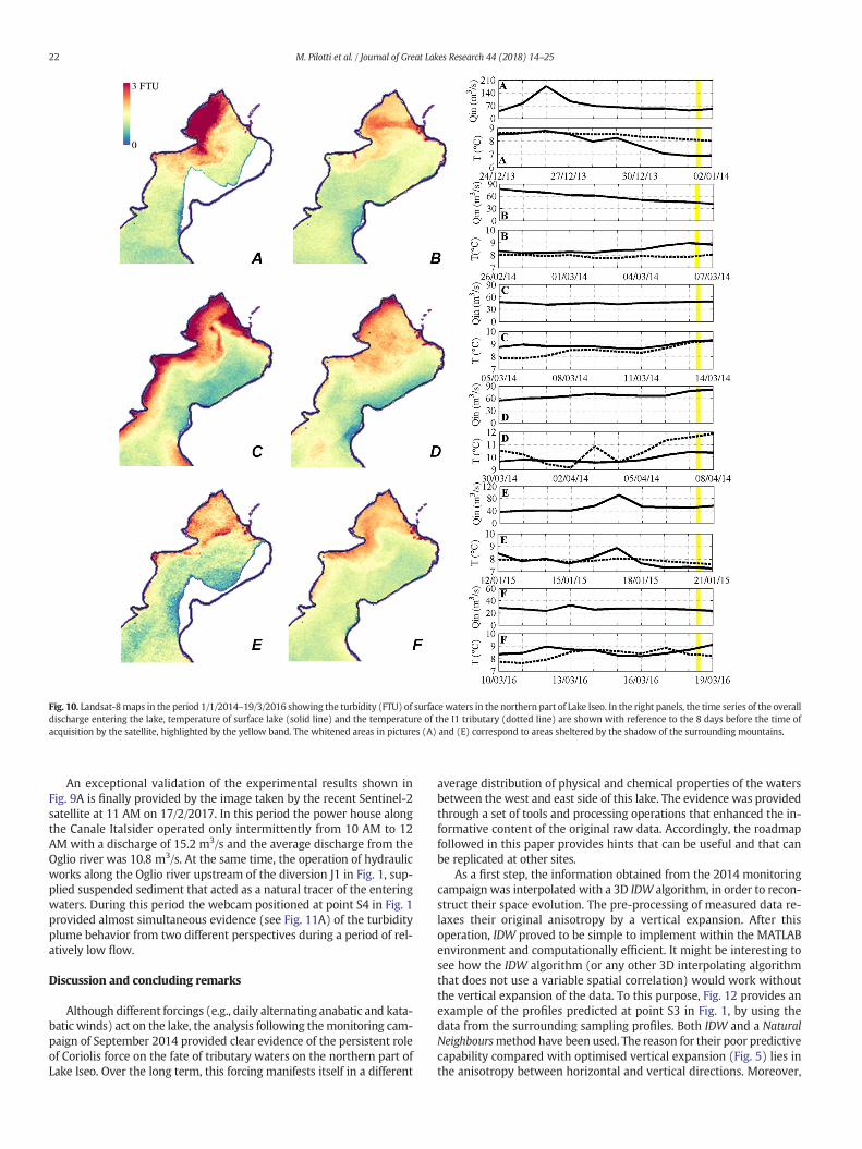
Fig. 10. Landsat-8maps in the period 1/1/2014–19/3/2016 showing the turbidity (FTU) of surface waters in the northern part of Lake Iseo. In the right panels, the time series of the overalldischarge entering the lake, temperature of surface lake (solid line) and the temperature of the I1 tributary (dotted line) are shown with reference to the 8 days before the time ofacquisition by the satellite, highlighted by the yellow band. The whitened areas in pictures (A) and (E) correspond to areas sheltered by the shadow of the surrounding mountains.

22 M. Pilotti et al. / Journal of Great Lakes Research 44 (2018) 14–25

An exceptional validation of the experimental results shown inFig. 9A is finally provided by the image taken by the recent Sentinel-2satellite at 11 AM on 17/2/2017. In this period the power house alongthe Canale Italsider operated only intermittently from 10 AM to 12AM with a discharge of 15.2 m3/s and the average discharge from theOglio river was 10.8 m3/s. At the same time, the operation of hydraulicworks along the Oglio river upstream of the diversion J1 in Fig. 1, sup-plied suspended sediment that acted as a natural tracer of the enteringwaters. During this period the webcam positioned at point S4 in Fig. 1provided almost simultaneous evidence (see Fig. 11A) of the turbidityplume behavior from two different perspectives during a period of rel-atively low flow.

Discussion and concluding remarks

Although different forcings (e.g., daily alternating anabatic and kata-batic winds) act on the lake, the analysis following themonitoring cam-paign of September 2014 provided clear evidence of the persistent roleof Coriolis force on the fate of tributary waters on the northern part ofLake Iseo. Over the long term, this forcing manifests itself in a different

average distribution of physical and chemical properties of the watersbetween the west and east side of this lake. The evidence was providedthrough a set of tools and processing operations that enhanced the in-formative content of the original raw data. Accordingly, the roadmapfollowed in this paper provides hints that can be useful and that canbe replicated at other sites.

As a first step, the information obtained from the 2014 monitoringcampaign was interpolated with a 3D IDW algorithm, in order to recon-struct their space evolution. The pre-processing of measured data re-laxes their original anisotropy by a vertical expansion. After thisoperation, IDW proved to be simple to implement within the MATLABenvironment and computationally efficient. It might be interesting tosee how the IDW algorithm (or any other 3D interpolating algorithmthat does not use a variable spatial correlation) would work withoutthe vertical expansion of the data. To this purpose, Fig. 12 provides anexample of the profiles predicted at point S3 in Fig. 1, by using thedata from the surrounding sampling profiles. Both IDW and a NaturalNeighboursmethod have been used. The reason for their poor predictivecapability compared with optimised vertical expansion (Fig. 5) lies inthe anisotropy between horizontal and vertical directions. Moreover,

Fig. 11. RGB images fromSentinel-2 (A) andwebcam (B) taken during thermally unstratifiedperiod at 11AMon 16/2/2017. The position of thewebcam is shown as S4 in Fig. 1. The overalldaily-averaged discharge entering the lake from I1 and I2 tributaries was 25m3/s; at 11 AM the hourly-averaged contribution from I1was 10.8m3/s, while the one from I2 was 15.2m3/s.

23M. Pilotti et al. / Journal of Great Lakes Research 44 (2018) 14–25

in the presence of layers with different density gradients, vertical corre-lation varies with depth.

As usual in this type of measurement, the considered data set is verydensely distributed along the vertical (data were measured every20 cm) but sparse in the horizontal (average distance between profileswas on the order of 300 m). Whenever data are spatially interpolated,an influence radius must be introduced under the assumption that cor-relation between measured values and the predicted one is negativelycorrelated with distance. If this radius is too small, the information ispoorly exploited because the neighborhood of the predicted point

Fig. 12. Example of measured (blue solid line) and predicted profiles at point S3 in Fig. 1. The prcomputed only on the basis of the data measured at the surrounding sampling profiles and wi

could be almost empty. Accordingly, the radius should be scaled onthe average distance between the measured profiles. However, this av-erage distance is typically larger than themaximumdepth and definite-ly larger than the length scale provided by the thermocline thickness ina thermally stratified lake, where the suppression of vertical turbulencecreates a strong horizontal correlation along the same isopotential sur-face. Accordingly, by using a 3D interpolation approach, the value of avariable interpolated at a given depth in the neighborhood of a mea-sured profile would be affected by the data measured along the verticalprofile, almost irrespective of depth. For instance, the predicted

edicted profiles (IDW algorithm, red line, and Natural Neighboursmethod, green line) arethout the optimised vertical expansion of the data as applied in Fig. 5.

Fig. 13. Turbiditymaps from Landsat-8 images obtained during thermally stratified periods (July 25, 2013 and July 1, 2016), when the average daily dischargewas comparable to the onesof Fig. 10.

24 M. Pilotti et al. / Journal of Great Lakes Research 44 (2018) 14–25

temperature at the thermocline would be almost equally affected bytemperature at the surface, at the bottom and at the thermocline of sur-rounding measured vertical profiles.

In such anenvironment, an effective 3D interpolation scheme shouldintroduce vertical anisotropy. The simplest way to do this is to segmentdata into layers, which is tantamount to repeatedly using a 2D interpo-lation approach that does not effectively utilize the measured informa-tion. This could be correct across the thermocline but could bequestionable in the mixed epilimnion above and in the hypolimnionbelow. Another possibility is using different correlation coefficientsalong vertical and horizontal directions. Finally, a simple approach isthe one introduced in this paper, that expands the distance of data inthe vertical direction during the prediction phase, sofictitiously creatinga lake whose horizontal direction is comparable to the vertical one.

One could expect that the layer thickness, the vertical correlation co-efficient, and the expansion coefficient should all vary with depth. Insuch a case, the expansion coefficient should change its value alongthe vertical as a function of the local stability of the water column,being maximum close to the thermocline and smaller in the surfacemixed layer and in the hypolimnion. To explore this, we have madesome attempts to link α to the local value of the buoyancy frequency,but without obtaining a conclusive benefit with respect to the use of asimple constant coefficient. Here, the most likely problem is that thelocal buoyancy frequency is in itself a function of the unknown temper-ature profile.

The physical model provided a vehicle to isolate the role of theCoriolis' force on the plume of the two tributaries, that is usually not vis-ible from the surface and is confounded with the combined effect ofother dynamic forcings (e.g., wind and the seiche related flow field).Under ordinary flow conditions, the model predicts a systematic deflec-tion of the tributary waters towards the western shore of the lake, trig-gering a clockwise gyre within the Lovere bay and a slow counter-clockwise gyre that returns water towards the river mouth movingalong the eastern shore. For higher flow rate discharges, the effect ofthe Earth's rotation weakens with respect to the plume's inertia in theentrance zone and it has a more rectilinear pattern. Accordingly, onecould expect that the north-western part of the lake, althoughmisaligned with respect to the tributaries axis, is systematically moresensitive to water quality degradation related to river-borne pollution.Suspended particles, containing nutrients and bacteria, could preferen-tially settle in this part of the lake, triggering metabolic processes thatcause a general reduction of the oxygen concentration along the watercolumns. This will increase the fragility of this area with respect to eu-trophication and algal blooms. Considering health risks associatedwith pollution of coastal bathing waters at the surface during the

summer, the prevailing interflow mode, that usually occurs at a depthbetween 5 and 10 m, probably contributes to diminishing the risk forthe north-western part of the lake but, on the basis of the obtained re-sults, a more specific modeling effort (e.g., Antenucci et al., 2005)seems necessary.

In spite of the discussed simplifying assumptions, the area ofinfluence of the tributaries deduced from the results of the physicalmodel closely matches the one shown by the remote sensing image(see Figs. 9A and 11A). Both these tools are easy to understand and tocommunicate; thus, providing effective instruments to convey the con-cept of the lake's vulnerability to a lay audience. Actually there is a cross-fertilization process between these two results: the first explains thereason for the patterns shown by the second, that, in turn, provides anevident confirmation of the correctness of the physical model.

In this study, we found that a physical explanation of the observedprocesses resulted from the coupling of analysis of the remote sensingimages with the other observations. The successful observation of theplume pattern in thermally unstratified periods would have been im-possible during the prevailing thermally stratified period, whose extentis known thanks to themeasurements of the lake and tributary temper-atures. As shown in Fig. 13, the images obtained in the thermally strat-ified period do not indicate clear evidence of the westward drift butusually only a higher level of diffused turbidity on the western side ofthe lake. This is probably the result of the vertical mixing exerted by in-ternal wave activity on the deeper tributary plumes. This underscoresthe importance of a stronger holistic approach coupling observations,experiments, and models in the investigation and understanding of re-mote sensing information.

Acknowledgments

This research is part of the ISEO (Improving the lake Status fromEutrophy to Oligotrophy) project and was made possible by a CARIPLOfoundation grant number 2015-0241. The participation of SCCwas sup-ported by the Summer Visiting Professor Programat theUniversità degliStudi di Brescia. We are grateful to Ilaria Cazzaniga and Chiara Elli forsupporting the satellite image processing. We are grateful to two anon-ymous Reviewers and to the Associate Editor for their contribution inthe improvement of this paper.

References

Antenucci, J.P., Brookes, J.D., Hipsey, M.R., 2005. A simple model for quantifying crypto-sporidium transport, dilution and potential risk in reservoirs. J. Am. Water WorksAssoc. 97, 86–93.

25M. Pilotti et al. / Journal of Great Lakes Research 44 (2018) 14–25

Atkinson, J.F., Lin, G., Joshi, M., 1994. Physical model of Niagara River discharge. J. GreatLakes Res. 20, 583–589.

Bahner, L., 2006. User Guide for the Chesapeake Bay and Tidal Tributary Interpolator.NOAA Chesapeake Bay Office, Annapolis, Md.

Bonomi, G., Gerletti, M., 1967. Il Lago d'Iseo: primo quadro limnologico generale (termica,chimica, plancton e benton pro- fondo). Mem. Ist. Ital. Idrobiol. 22, 149–175.

Bouffard, D., Perga, M.E., 2016. Are flood-driven turbidity currents hot spots for primingeffect in lakes? Biogeosciences 13 (3573–3584), 2016.

Brando, V.E., Braga, F., Zaggia, L., Giardino, C., Bresciani, M., Bellafiore, D., Ferrarin, C.,Maicu, F., Benetazzo, A., Bonaldo, D., Falcieri, F.M., Coluccelli, A., Russo, A., Carniel,S., 2015. High resolution satellite turbidity and sea surface temperature observationsof river plume interactions during a significant flood event. Ocean Sci. Discuss. 11,909–920.

Chapra, S.C., 1997. Surface Water Quality Modeling. McGraw Hill.Chen, X., Driscoll, C.T., 2009. Watershed land use controls on chemical inputs to Lake On-

tario embayments. J. Environ. Qual. 38, 2084–2095.Chen, C., Wang, L., Ji, R., Budd, J.W., Schwab, D.J., Beletsky, D., Fahnenstiel, G.L.,

Vanderploeg, H., Eadie, B.J., Cotner, J.B., 2004. Impacts of suspended sediment onthe ecosystem in Lake Michigan: a comparison between the 1998 and 1999 plumeevent. J. Geophys. Res. 109, C10S05 (18 pp.).

Chipman, J.W., Lillesand, T.M., Schmaltz, J.E., Leale, J.E., Nordheim, M.J., 2004. Mappinglake water clarity with Landsat images in Wisconsin, U.S.A. Can. J. Remote. Sens. 30(1):1–7. https://doi.org/10.5589/m03-047.

Chomicki, K.M., Howell, E.T., Defield, E., Dumas, A., Taylor, W.D., 2016. Factors influencingthe phosphorus distribution near the mouth of the Grand River, Ontario, Lake Erie.J. Great Lakes Res. 42 (3), 549–564.

Dogliotti, A.I., Ruddick, K.G., Nechad, B., Doxaran, D., Knaeps, E., 2015. A single algorithmto retrieve turbidity from remotely-sensed data in all coastal and estuarine waters.Remote Sens. Environ. 530 (156):157–168. https://doi.org/10.1016/j.rse.2014.09.020.

European Parliament, 2000. Directive 2000/60/EC of the European Parliament and of theCouncil of 23 October 2000 Establishing a Framework for Community Action in theField of Water Policy.

Fink, G., Wessels, M., Wüest, A., 2016. Flood frequency matters: why climate change de-grades deep-water quality of peri-alpine lakes. J. Hydrol. (ISSN: 0022-1694) 540:457–468. https://doi.org/10.1016/j.jhydrol.2016.06.023 (September 2016).

Foley, J.D., van Dam, A., Hughes, J.F., Feiner, S.K., 1990. Spatial-partitioning representa-tions; surface detail. Computer Graphics: Principles and Practice. The Systems Pro-gramming Series. Addison-Wesley, Boston. ISBN: 0-201-12110-7.

Griffiths, R.W., 1986. Gravity currents in rotating systems. Annu. Rev. Fluid Mech. 18,59–89.

Hakanson, L., 1974. Mercury in some Swedish lake sediments. Ambio 3, 37–43.Hakanson, L., Janson, M., 1983. Principles of Lake Sedimentology. Springer, Berlin,

Germany.Halder, J., Decrouy, L., Vennemann, T.W., 2013. Mixing of Rhône River water in Lake

Geneva (Switzerland–France) inferred from stable hydrogen and oxygen isotopeprofiles. J. Hydrol. (ISSN: 0022-1694) 477:152–164. https://doi.org/10.1016/j.jhydrol.2012.11.026 (16 January 2013).

Hamblin, R.E., Carmack, E.C., 1978. River-induced currents in a fjord lake. J. Geophys. Res.63, 885–899.

Hogg, C.A.R., Marti, C.L., Huppert, H.E., Imberger, J., 2013. Mixing of an interflow into theambient water of Lake Iseo. Limnol. Oceanogr. 58 (2):579–592. https://doi.org/10.4319/lo.2013.58.2.0579.

Kreling, J., Bravidor, J., Engelhardt, C., Hupfer, M., Koschorreck, M., Lorke, A., 2016. The im-portance of physical transport and oxygen consumption for the development of ametalimnetic oxygen minimum in a lake. Limnol. Oceanogr. https://doi.org/10.1002/lno.10430.

Laborde, S., Antenucci, J.P., Copetti, D., Imberger, J., 2010. Inflow intrusions at multiplescales in a large temperate lake. Limnol. Oceanogr. 55, 1301–1312.

Lathrop Jr., R.G., Vande Castle, J.R., Lillesand, T.M., 1990. Monitoring river plume transportand mesoscale circulation in Green Bay Lake Michigan USA through satellite remotesensing. J. Great Lakes Res. 16 (3), 471–484.

Li, J., Heap, A.D., 2011. A review of comparative studies of spatial interpolation methods inenvironmental sciences: performance and impact factors. Ecol. Inform. 6 (2011),228–241.

Li, C., Kisser, K.M., Rumer, R.R., 1975. Physical model study of circulation patterns in LakeOntario. Limnol. Oceanogr. 203, 323–337.

Li, C., Walker, N., Hou, A., Georgiou, I., Roberts, H., Laws, E., McCorquodale, J.A., Weeks, E.,Li, X., Crochet, J., 2008. Circular plumes in Lake Pontchartrain estuary under windstraining. Estuarine Coast. Shelf Sci. (ISSN: 0272-7714) 80 (1):161–172. https://doi.org/10.1016/j.ecss.2008.07.020.

Li,W., Liu,W.L., Zhang, Y., Yin, W., Liu, Y., 2010. On the comparison of spatial interpolationmethods ofmarine temperature and salinity based on ARGIS software: a case study ofTianjin coastal waters in the Bohai Bay. In: Guo, H., Wang, C. (Eds.), Sixth Internation-al Symposium on Digital Earth: Models, Algorithms, and Virtual Reality, Beijing,People's Republic of China. SPIE Press, Bellingham, WA.

Li, J., Heap, A.D., Potter, A., Daniell, J.J., 2011. Application of machine learning methods tospatial interpolation of environmental variables. Environ. Model Softw. 12 (26),1647–1659.

Morillo, S., Imberger, J., Antenucci, J.P., Woods, P.F., 2008. The influence of wind and LakeMorphometry on the interaction between two rivers entering a stratified lake.J. Hydraul. Eng. 134, 1579–1589.

Mortimer, C.H., 2006. Inertial oscillations and related internal beat pulsations and surgesin Lakes Michigan and Ontario. Limnol. Oceanogr. 51 (5), 1941–1955.

Murphy, R., Curriero, F., Ball, W., 2010. Comparison of spatial interpolation methods forwater quality evaluation in the Chesapeake Bay. J. Environ. Eng.:160–171 https://doi.org/10.1061/(ASCE)EE.1943-7870.0000121.

Özkundakci, D., Hamilton, D.P., Kelly, D., Schallenberg, M., De Winton, M., Verburg, P.,Trolle, D., 2014. Ecological integrity of deep lakes in New Zealand across anthropo-genic pressure gradients. Ecol. Indic. 37, 45–57.

Pahlevan, N., Lee, Z., Wei, J., Schaaf, C.B., Schott, J.R., Berk, A., 2014. On-orbit radiometriccharacterization of OLI (Landsat-8) for applications in aquatic remote sensing. Re-mote Sens. Environ. 154:272–284. https://doi.org/10.1016/j.rse.2014.08.001.

Pilotti, M., Valerio, G., Leoni, B., 2013. Data set for hydrodynamic lake model calibration: adeep pre-Alpine case. Water Resour. Res. 49:7159–7163. https://doi.org/10.1002/wrcr.20506.

Pilotti, M., Valerio, G., Gregorini, L., Milanesi, L., Hogg, C., 2014a. Study of tributary inflowsin Lake Iseo with a rotating physical model. J. Limnol. 73 (1). https://doi.org/10.4081/jlimnol.2014.772.

Pilotti, M., Simoncelli, S., Valerio, G., 2014b. A simple approach to the evaluation of the ac-tual water renewal time of natural stratified lakes. Water Resour. Res. 50 (4):2830–2849. https://doi.org/10.1002/2013WR014471.

Rumer, R.R., Robson, L., 1968. Circulation Studies in a Rotating Model of Lake Erie. StateUniversity of New York at Buffalo (36 pp.).

Sahlin, J., Mostafavi, M.A., Forest, A., Babin, M., 2014. Assessment of 3D spatial interpola-tion methods for study of the marine pelagic environment. Mar. Geod. 37 (2):238–266. https://doi.org/10.1080/01490419.2014.

Stewart, K.M., 1988. Tracing inflows in a physical model of Lake Constance. J. Great LakesRes. 14 (466), 478.

Strömbeck, N., Pierson, E., 2001. The effects of variability in the inherent optical propertieson estimations of chlorophyll a by remote sensing in Swedish freshwater. Sci. TotalEnviron. 268, 123–137.

Toming, K., Kutser, T., Laas, A., Sepp, M., Paavel, B., Nõges, T., 2016. First experiences inmapping lake water quality parameters with sentinel-2 MSI imagery. Remote Sens.8 (8), 640.

USEPA, Region III Water Protection Division, 2007. Ambient water quality criteria for dis-solved oxygen, water clarity and chloro-phyll a for the Chesapeake Bay and its tidaltributaries 2007 addendum. Rep. No. EPA 903-R-07-003, U.S. Environmental Protec-tion Agency Region III, Chesapeake Bay Program Office, and Region III Water Protec-tion Division, Annapolis, Md.

Valerio, G., Pilotti, M., Marti, C.L., Imberger, J., 2012. The structure of basin scale internalwaves in a stratified lake in response to lake bathymetry and wind spatial and tem-poral distribution: Lake Iseo, Italy, Limnol. Oceanography 57 (3), 772–786.

Vanhellemont, Q., Ruddick, K., 2014. Turbid wakes associated with offshore wind turbinesobserved with Landsat 8. Remote Sens. Environ. 145:105–115. https://doi.org/10.1016/j.rse.2014.01.009.

Vanhellemont, Q., Ruddick, K., 2015. Advantages of high quality SWIR bands for oceancolour processing: examples from Landsat-8. Remote Sens. Environ. 161:89–106.https://doi.org/10.1016/j.rse.2015.02.007.

Wetzel, R.G., 1992. Clean water: a fading resource. Hydrobiologia 243, 21–30.Wetzel, R.G., 2001. Limnology. 3rd ed. Academic Press.Wright, R.F., Nydegger, P., 1980. Sedimentation of detrital particulate matter in lakes: in-

fluence of currents produced by inflowing rivers. Water Resour. Res. 16, 597–601.Zhang, Y., Shi, K., Zhou, Y., Liu, X., Qin, B., 2016. Monitoring the river plume induced by

heavy rainfall events in large, shallow, Lake Taihu using MODIS 250 m imagery. Re-mote Sens. Environ. 173, 109–121.

Zimmerman, D., Pavlik, C., Ruggles, A., Armstrong, M.P., 1999. An experimental compari-son of ordinary and universal kriging and inverse distance weighting. Math. Geol. 31(4), 375–390.