journal of la a mathematical model to study the dynamics
TRANSCRIPT
JOURNAL OF LATEX CLASS FILES, VOL., NO., JANUARY 2011 1
A Mathematical Model to study theDynamics of Epithelial Cellular Networks
Alessandro Abate, Member, IEEE, Stephane Vincent, Roel Dobbe,Alberto Silletti, Member, IEEE, Neal Master, Jeffrey D. Axelrod, and Claire J. Tomlin, Fellow, IEEE
Abstract—Epithelia are sheets of connected cells that are essential across the animal kingdom. Experimental observations suggestthat the dynamical behavior of many single-layered epithelial tissues has strong analogies with that of specific mechanical systems,namely large networks consisting of point masses connected through spring-damper elements and undergoing the influence of activeand dissipating forces. Based on this analogy, this work develops a modeling framework to enable the study of the mechanical propertiesand of the dynamic behavior of large epithelial cellular networks. The model is built first by creating a network topology that is extractedfrom the actual cellular geometry as obtained from experiments, then by associating a mechanical structure and dynamics to thenetwork via spring-damper elements. This scalable approach enables running simulations of large network dynamics: the derivedmodeling framework in particular is predisposed to be tailored to study general dynamics (for example, morphogenesis) of variousclasses of single-layered epithelial cellular networks. In this contribution we test the model on a case study of the dorsal epithelium ofthe Drosophila melanogaster embryo during early dorsal closure (and, less conspicuously, germband retraction).
Index Terms—Epithelium, Cellular network, Nonlinear dynamical model, Spring-damper system, Discrete element method, Earlydorsal closure, Morphogenesis
F
1 INTRODUCTION
QUANTITATIVELY understanding the mechanicalstructure and dynamical properties of epithelial
cellular networks is a compelling but complex task.Three main factors contribute to the difficulty of thisgoal.
Firstly, single cells are made up of a number of distinctcomponents, each contributing to their mechanical struc-ture [1]. The mechanical characteristics of networks ofcells thus hinge on the characteristics of single cells, eachwith their complex structural features [2]. Encompassingthese components easily leads to high-dimensional, non-linear, spatially distributed models of cellular networksthat are not likely to be prone to mathematical analy-sis or to simulation on a computer over large cellularnetworks.
Secondly, at the cellular network level, dynamics areoften influenced by a combination of different forces
• A. Abate and R. Dobbe are with the Delft Center for Systems and Control,TU Delft, Delft, The Netherlands. E-mail: [email protected]
• S. Vincent is with the Ecole Normale Superieure de Lyon, Lyon, France. E-mail: [email protected]
• A. Silletti is with the Department of Information Engineering, Universityof Padova, Padova, Italy. E-mail: [email protected]
• J.D. Axelrod is with the Department of Pathology, Stanford UniversitySchool of Medicine, Stanford, CA, USA. E-mail: [email protected]
• N. Master and C.J. Tomlin are with the Department of Electrical Engineer-ing and Computer Sciences, University of California at Berkeley, Berkeley,CA, USA. E-mail: {neal.m.master, tomlin}@EECS.berkeley.EDU
The first three authors have equally contributed to this work. This researchis in part funded by grants R01 GM097081 and R01 GM097081, by NCIthrough the PSOC grant, by the European Commission under the NoEFP7-ICT-2009-5 257462, by the European Commission under Marie Curiegrant MANTRAS PIRG-GA-2009-249295, by NWO under VENI grant016.103.020.
(both internal and external to the network) acting si-multaneously [3], [4], [5] – isolating individual forcemechanism contributions in the lab can be a dauntingtask – we contend that a synthetic model can be analternative solution.
Thirdly, the influence of genetic processes on the me-chanical properties of cellular network is currently anopen field of investigation [6]: conducting manipulationsin the expression of certain genes can lead to significantlydifferent mechanical properties. Encompassing such adependence at the modeling level can be very difficult.
This work focuses on the first two of the three issuesdescribed above. With the general goal of developinga quantitative model comes a tradeoff between modeldescriptiveness and precision on the one hand, and size,computability, and ease of analysis on the other. Takingup this latter perspective, the main objective of thiswork is to develop a quantitative mathematical modelfor the study of the dynamics of large and heterogeneousepithelial networks. The model furthermore enables theinvestigation of the role played by forces acting onthe epithelium, as well as the study of the influenceof the non-uniformity of its mechanical properties onits dynamics. The model is developed with the mainintention of enabling the simulation of complex, large-dimensional networks of cells.
After benchmarking two different modeling ap-proaches over their ability to encompass the complexityof epithelial networks and the capacity of modelingsubtleties of single cellular mechanics, this work presentsa model that strikes a balance between computable high-level abstractions [7], [8], [9], [10] and specific low-levelrefined characterizations [11], [12], [13]. We claim that the
JOURNAL OF LATEX CLASS FILES, VOL., NO., JANUARY 2011 2
main features of the proposed modeling framework arethat 1. it is biologically well-grounded; 2. it is tractablefor analysis and large-scale simulations; and 3. it ispromising in a number of diverse applications focusingon classes of single-layered epithelial cellular networks.
Structure of the articleSection 2 recapitulates biological knowledge that is at thebasis of cellular mechanics. Based on this insight, Section3 proposes important modeling criteria and distills themtowards the derivation of a novel modeling frameworkfor single-layered epithelial cellular networks. This partmotivates the use of the discrete-element approach asa principal constituent of the model. This Section alsoelaborates on the mathematical formulation: first, theunderlying graphical structure is described; then, thedynamics are associated to the structure by introducingspring-damper elements. Section 4 discusses the po-tentials and the limitations of the proposed modelingframework. While this work does not claim to lead toany new biological insight, with the goal of validatingthe approach Section 5 proposes a experimental study,which focuses on simulating the dorsal epithelium ofD. melanogaster embryo during early dorsal closure (andin part germband retraction). Section 5.1 presents howexperimental data is utilized as a basis for the modelingframework (definition of the graphical structure). Sec-tion 5.2 discusses how the dynamics are added to themodel, as well as how external forces and constraints areincluded. Section 5.3 presents the outcomes of the sim-ulations: it focuses on both qualitative and quantitativeassessments of modeling properties and of simulationassumptions. Finally, Section 6 concludes the work.
2 BIOLOGICAL BACKGROUND
This Section recalls key empirical evidence on cellularmechanics. In order to gain understanding on its me-chanical and dynamical characteristics, a single epithelialcell is dissected in terms of its own structural compo-nents and of its connections to adjacent components.
2.1 Cellular MechanicsCells are highly dynamic: they stretch, crawl, changeshape and divide [14]. Their mechanical properties de-pend on their internal structure [15]. In many criticalbiological processes, cells both exert and respond toforces toward and from their surroundings [16]. Themechanical properties of a cell are thus intimately relatedto its physical nature, as well as to its position within anetwork of similar cells.
Cellular mechanics are determined by three key as-pects: the internal structure of the cells, which hinges onthe presence of the cytoskeleton (Sec. 2.1.1); cell-cell con-nections within the epithelium, as well as the connectionof epithelial cells to other tissue layers (Sec. 2.1.2); andtwo additional important mechanical characteristics [16],[17]: nonlinear elasticity and anisotropy (Sec. 2.1.3).
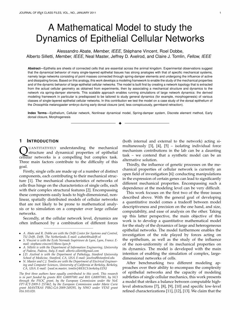
2.1.1 Cellular structureThe cytoskeleton is a complex, heterogeneous and dy-namic structure, which affects both elastic and viscouscharacteristics of cells [8], [18], [19], [20] (for possiblemodeling frameworks to encompass these properties see[10], [21], [22], [23]). The cytoskeleton is a biopolymernetwork consisting of three major components (Figure1): microfilaments (made of actin), intermediate fila-ments, and microtubules. In addition to these majorcomponents, a myriad of filament cross-linker, motorand regulatory proteins also play a role.
cell membrane
circumferential actin belts
(a) Cell membrane (thin, black) and circumferen-tial actin belts along the cell boundaries (thick,blue).
adherens junctions(E-cadherin/integrin connections)
intermediate filaments
microtubules
(b) Intermediate cytoskeletal components (fila-ments and microtubules) and cell-cell connections(adherens junctions).
Fig. 1. Pictorial top-view of a single cell in an epithelialnetwork.
Cell tensional forces depend on the three componentsmentioned above [24]. With regards to the first filaments,actin accumulates as a circumferential belt along the cellmembrane, at a specific apical-basal depth. Circumfer-ential actin belts of adjacent cells are connected to eachother through adherens junctions, see Figures 1(b) and2, which thus contribute to cytoskeletal structure anddynamics by connecting cytoskeleta of adjacent cells. Anadherens junction is a cell junction whose cytoplasmic
JOURNAL OF LATEX CLASS FILES, VOL., NO., JANUARY 2011 3
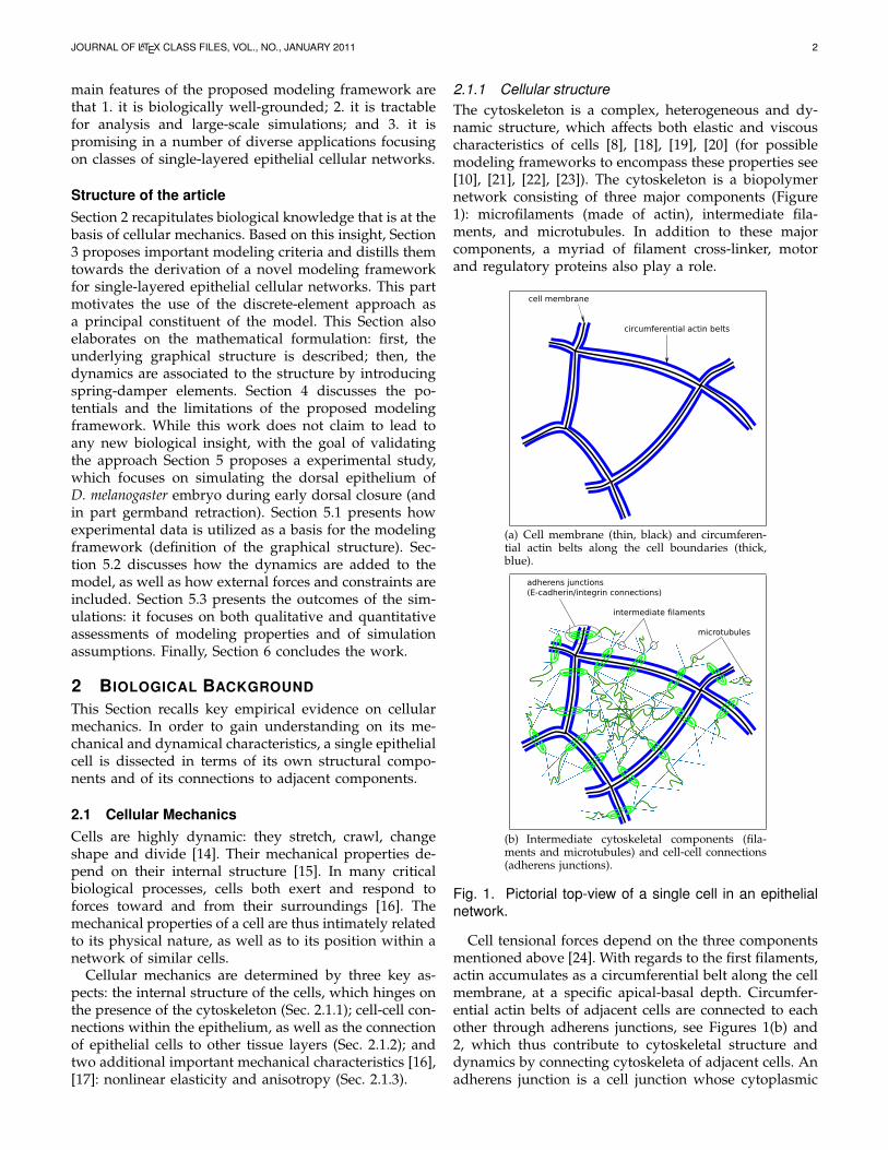
face is linked to the cytoskeleton. The connection ofcircumferential actin belts of adjacent cells creates atwo-dimensional network of actin, within the epithelialcellular network.
Fig. 2. Two-dimensional pictorial top-view of two ad-jacent epithelial cells: actin accumulation (blue) alongcell boundaries (black outer lines). Adherens junctions(green) connect different circumferential actin bundlesbetween the cytoskeleta of adjacent cells along theirboundaries.
As for intermediate filaments, they operate as ropesconnecting two points on the cell membrane. They forma pattern of intersecting lines over the cell, as depictedin Figure 1(b). The tension sustaining actin filamentsis balanced by interconnected structural elements thatbear compression, called microtubules [25], with Theflexible protein structure [9]. They act as struts pushingthe cell membrane outwards, as depicted in Figure 1(b).Pushing microtubules and pulling intermediate actinfilaments meet at the cell membrane, around adherensjunctions, contributing together with actin belts to cellshape stability.
While the discussion has focused on the two-dimensional surface of circumferential actin belts andthe elements in between, there also exist cytoskeletalcomponents connecting the apical and basal cell mem-branes, thus developing along the third dimension of thecell (the apical-basal axis, which crosses the cell surface).These filaments govern the stability of the thickness ofthe cell under stretching and compressing loads.
While recent studies have addressed the issue ofmodeling the thickness of epithelial cells [2], [26], sincein epithelia much of the mechanical properties of cellnetworks is dictated by the cell apical surface, a two-dimensional simplification is a good compromise thatcaptures many of the properties of interest. Also inthe present study, we shall focus on two-dimensionalcellular properties and argue that, under careful workingassumptions, the effect of this third dimension can be leftout.
2.1.2 Cell-cell connections and connection to the extra-cellular matrixThe different cytoskeletal components of adjacent cellsare connected by junctions (Figures 1(b) and 2), whichare composed of (among others) integrin and E-cadherinproteins. These proteins are cell adhesion moleculesnestled in the cell membrane and are connected to
cell adhesion molecules of neighboring cells [27] (seeSection 2.1.2), creating a cellular aggregate. The celladhesion molecules can float through the cell membraneplane, which suggests that the bilipid cell membranedoes not play a significant contribution to the structuralbalance of the cell. Most of the force is sustained bycytoskeletal components that cross cell membranes. Indeveloping epithelia, cell junctions often rearrange at ahigh frequency, which facilitates cell motility and cellproliferation. In many other cases – with a much lowerfrequency – rearrangements help stabilizing the epithe-lium. Because epithelia serve primarily as a structurallayer to protect underlying organs and processes, stableadherens junctions are needed to seal cells together intoan aggregate. In this work we shall focus on cellular net-works where rearrangements have very low occurrenceand thus can be disregarded.
The extracellular matrix, and more specifically thebasement membrane, is situated underneath the epithe-lium. Epithelial cellular networks are connected to theextracellular matrix [18], particularly to the basementmembrane via focal adhesions, where integrins serveas anchors [27]. The number of adhesions affects thedynamical characteristic of this viscous interaction.
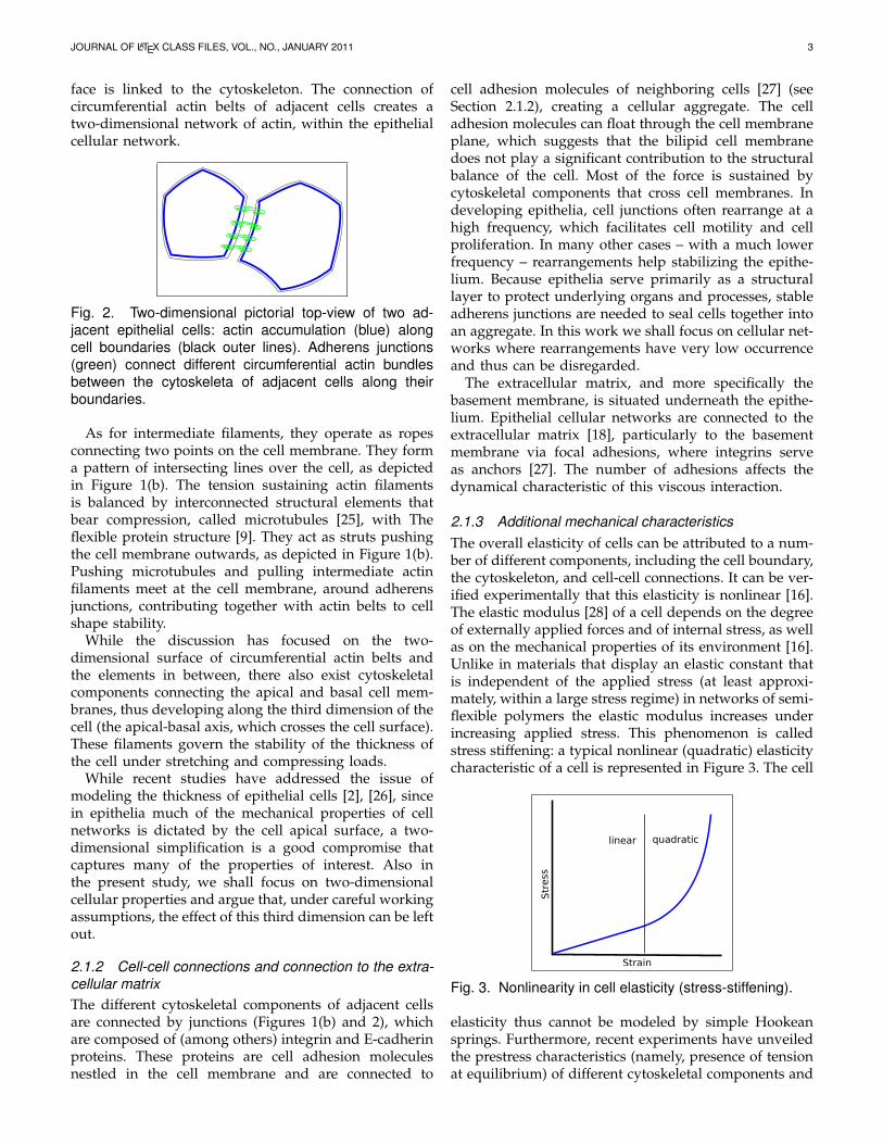
2.1.3 Additional mechanical characteristicsThe overall elasticity of cells can be attributed to a num-ber of different components, including the cell boundary,the cytoskeleton, and cell-cell connections. It can be ver-ified experimentally that this elasticity is nonlinear [16].The elastic modulus [28] of a cell depends on the degreeof externally applied forces and of internal stress, as wellas on the mechanical properties of its environment [16].Unlike in materials that display an elastic constant thatis independent of the applied stress (at least approxi-mately, within a large stress regime) in networks of semi-flexible polymers the elastic modulus increases underincreasing applied stress. This phenomenon is calledstress stiffening: a typical nonlinear (quadratic) elasticitycharacteristic of a cell is represented in Figure 3. The cell
linear quadratic
Strain
Stress
Fig. 3. Nonlinearity in cell elasticity (stress-stiffening).
elasticity thus cannot be modeled by simple Hookeansprings. Furthermore, recent experiments have unveiledthe prestress characteristics (namely, presence of tensionat equilibrium) of different cytoskeletal components and
JOURNAL OF LATEX CLASS FILES, VOL., NO., JANUARY 2011 4
of the cell as a whole [20], [25], [29]. Evidence (both atthe cellular [15], [29] and cytoskeletal level [19], [25])has shown a linear relation between pre-stress and thestiffness coefficient. Following the analogy with springelements exerting forces proportional to stiffness andstrain, this results in a quadratic elasticity characteristic.Furthermore, by severing individual actin filaments andmicrotubules and analyzing the dynamical response ofthe cell, it was shown that the dynamical characteris-tics of cytoskeletal components are viscoelastic. Theseresponses can be encompassed by leveraging the Voigtelement [30], which employs a spring and a damper inparallel (see also Sec. 3.4 for the mathematical detailsand Sec. 4.1 for alternatives or extensions).
The spatial organization of cytoskeletal compo-nents creates cellular structures which are inherentlyanisotropic. For instance, microtubules often determinethe direction of elongation of a cell [17]. A feature ofstretched cells is the alignment of their cell boundaries.Hence, the circumferential actin filaments that organizealong the cell membrane, tend to sustain and propagatemost of the load in the network. This property of thecell boundaries, in addition to the discussed nonlinearelasticity behavior, contribute to the cell stability.
3 MODELING FRAMEWORK
Section 3.1 distills the details on cellular mechanicsdiscussed in the previous section into a few essentialmodeling criteria for single-layer epithelial cellular net-works. Among the many cellular modeling alternativesin the literature [2], Section 3.2 motivates the modelingchoices by comparison against one alternative knownmodeling framework. Section 3.3 describes the under-lying structure of the model. This leads to the formalintroduction of the dynamical modeling framework inSection 3.4.
3.1 Modeling principles
We synthesize the biological knowledge presented inSection 2 into the following key principles, which in-spire the development of a model for epithelial cellularnetworks:
1) The cellular architecture is discrete:Single epithelial cells behave mechanistically asdiscrete entities composed of different intercon-nected cytoskeletal constituents, and are able tosustain both tensional and compressional loads.They do not behave as mechanical (viscous orviscoelastic) continua. The discrete nature of theactin network and of intermediate filaments shouldbe incorporated in the model. A large proportionof the actin architecture is organized over a two-dimensional surface, governing most of the ob-served cell dynamics [31], [32].
2) Anisotropy depends both on cell geometry and on net-work topology:
Single cells have highly anisotropic mechanicalstructures, determined by their physical character-istics as well as by their geometry. Along with localanisotropy, the network topology is often necessaryto explain the existence of global properties orcertain global dynamics, such as the alignmentof patches of cells or the propagation of forcesthrough the cellular network. Taking into accountboth single cell geometry and global topology ofthe epithelial network is therefore necessary tostudy anisotropy and to explain properties at thenetwork level.
3) Nonlinear and temporal mechanical characteristics ofcell appear due to different structural components:Cell components display characteristics of nonlin-ear elasticity, which thus emerges at the cellu-lar level. The cytoskeletal prestress contributes tothe nonlinearity in cell deformation [19], [20] andshould be integrated with ideas from the tensegritymodel [24]. Relatively simple nonlinear elasticitycharacteristics (namely, quadratic relations) havebeen observed at a cellular level as well as over alarger tissue level [16], [25], [29]. Furthermore, morecomplex properties (hysteresis, memory) can playa role in specific instances, thus the model shouldbe extensible to accommodate them.
4) Modeling volume preservation can be complex:Volume preservation is a feature of epithelial cellsdeforming in a network. However, since there isno clear relation between the stress in the surfacedirections (planar dimension) and the thickness(height) of the cellular network [26], volume preser-vation of cellular components should be imposedunder controlled conditions and over specific spa-tial models.
3.2 Comparison between FEM and DEM modelsFinite and discrete element methods (FEM and DEM)are numerical techniques developed to compute approx-imate solutions of partial differential equations (PDE)and of integral equations [30], [33]. These methods are inparticular used for solving a set of nonlinear PDE overtime-varying domains whenever the desired precisionvaries over the entire domain, or in case the solutionlacks smoothness. The common feature of these twotechniques is the application of a mesh discretization ofa continuous domain into a set of discrete sub-domains,called elements. We draw a qualitative comparison be-tween FEM and DEM techniques. This comparison isattuned to the modeling principles explained above and,with focus on the problem under study, is intended tomotivate the choice of DEM as the basis of the model.
FEM represent continuous objects by meshing theminto volumetric elements. Within each of these elementsthe mechanical properties are defined as constant orcontinuous functions. When spatial properties such asincompressibility, osmotic pressure, or density are im-portant, then using these elements is indispensable.

JOURNAL OF LATEX CLASS FILES, VOL., NO., JANUARY 2011 5
The FEM approach assumes that strain and stress varycontinuously over the introduced volumetric elements,which is a delicate assumption when modeling systemsendowed with a discrete mechanical structure.
DEM on the other hand consider a nodal mesh ofa given object, in which nodes are associated to pointmasses and connected via discrete elements (discrete el-ements can be specific mechanical components). Internalforces can be exerted in any direction between nodes.The DEM approach is useful when the presence andorganization of distinct elements resembles the physicalstructure of the system.
Hybrid combinations with both element types are alsopossible [22], for instance on structures consisting ofbeams (modeled with volumetric finite elements) androds (modeled with discrete elements).
The four criteria derived in Section 3.1 are used tocompare the two modeling methods in Table 1. For eachof the criteria, the table includes a simple assessment(positive vs. negative sign) of the two modeling frame-works. The DEM approach is selected as the basis of themodel that will be developed in Section 3 for the follow-ing reasons. The DEM method is suited to easily repre-sent the discrete tensegrity structure of cellular mechan-ics. The use of DEM also enables the study of anisotropydue to cellular geometry and structural organization(network topology). Cellular volume preservation is anelusive task (though FEM techniques may enable en-compassing it), and therefore is not considered in theearly stage of modeling framework development. TheDEM has shown interesting results in other modelingstudies, where nonlinear mechanical characteristics wereincorporated. These studies showed qualitative resem-blance of tissue deformation [34], [35], [36] and displayedstability properties over high-dimensional models [37].Time-dependent properties (hysteresis, memory effects)can be incorporated, albeit at increased computationalcosts. In conclusion, DEM promises to encompass thefeatures of interest for the problem at hand.
3.3 Graphical representation of underlying cellularstructure
Consider a general graph-theoretical structure. Thisstructure will be generated from experimental data, asdiscussed in Section 5.1. The graph consists of threedifferent features: vertices, edges, and faces. Vertices arecontained in a set V of cardinality N , which stores theindex i ∈ {1, 2, . . . , N} of each vertex vi. In Figure 4 ver-tices are indicated by dots and their indices are denotedby the adjacent numbers. An edge (circled numbers inFigure 4) ei,j = {vi, vj} is defined as a pair of adjacentvertices vi and vj , where j 6= i and i, j ∈ {1, 2, . . . , N}.Edges are stored as pairs in a N e × 2 set E, where N e isthe cardinality of set E. The edge index k ∈ {1, 2, . . . , N e}is defined by the row number in E. The graph G = (V,E)describes the full topology of a network. Consider theN × N e incidence matrix H of a graph. Its entries are
TABLE 1Comparison of FEM and DEM modeling frameworks.
1) Cellular architecture is discreteFEM DEM
± Representation of discretetensegrity structureunclear
+ Can represent discretetensegrity structure
+ Can be combined withDEM as a hybrid model
- To keep computationstractable, number ofcomponents per cell islimited to a lumped versionof the real cell layout
2) Anisotropy also depends on cell geometry and network topologyFEM DEM
+ Finite elements can beadapted to cellulargeometry
+ Discrete elements can beadapted to cellulargeometry
± Incorporation ofanisotropy of actinaccumulation bundles tobe understood
+ Anisotropy of actinaccumulation bundles caneasily be incorporated
- Computational issuesrelated to modeling largescale cellular networks
+ Can scale to model largecellular networks and thusencompass their topologicalfeatures
3) Nonlinear and temporal mechanical characteristicsFEM DEM
+ Can be incorporated infinite elements
+ Can be incorporated indiscrete elements
- May lead to heavycomputations, even foraverage-sized cellularnetwork
+ Nonlinear elasticityqualitatively resemblestissue deformation
+ Nonlinear elasticitycontributes to modelstability, prevents collapse
- Temporal characteristics canbe computationallydemanding
4) Volume preservationFEM DEM
+ Can be imposed throughvolumetric properties
± Its effect can beapproximated but notformally embedded
± May result in artifactsand computational issues(stiffness), due to limitedknowledge on propertiesof cell height
- Approximation likelyrelated to introduction ofdynamical artifacts, requiresevaluation of resultingmechanical properties
formulated as
hik =
+1, if vi is the first component of kth edge−1, if vi is the second component of kth edge
0, otherwise.
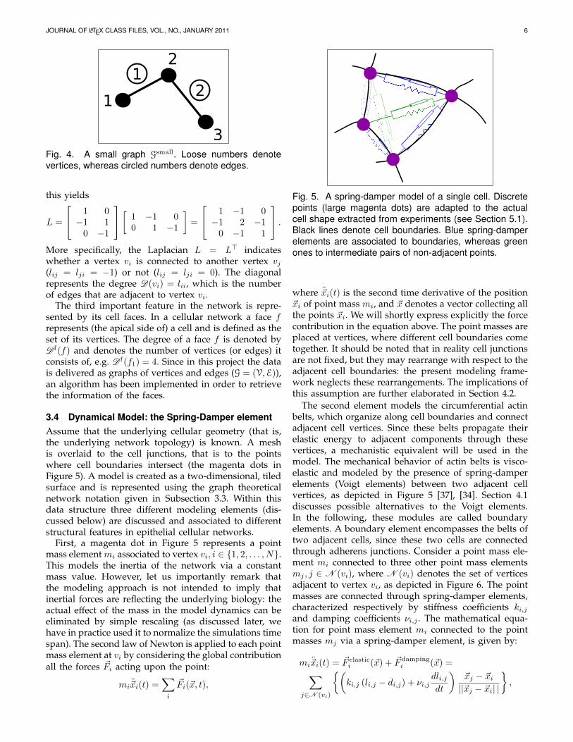
As an example, consider a small graph Gsmall consistingof three vertices and two edges, as depicted in Figure 4.The incidence matrix follows:
H =
1 0−1 1
0 −1
.The N ×N Laplacian matrix L describes which verticesare adjacent to each other and is calculated using theincidence matrix [38], as given by L = HH>. For Gsmall
JOURNAL OF LATEX CLASS FILES, VOL., NO., JANUARY 2011 6
3
2
1
12
Fig. 4. A small graph Gsmall. Loose numbers denotevertices, whereas circled numbers denote edges.
this yields
L =
1 0−1 1
0 −1
[ 1 −1 00 1 −1
]=
1 −1 0−1 2 −1
0 −1 1
.More specifically, the Laplacian L = L> indicateswhether a vertex vi is connected to another vertex vj(lij = lji = −1) or not (lij = lji = 0). The diagonalrepresents the degree D(vi) = lii, which is the numberof edges that are adjacent to vertex vi.
The third important feature in the network is repre-sented by its cell faces. In a cellular network a face frepresents (the apical side of) a cell and is defined as theset of its vertices. The degree of a face f is denoted byD f(f) and denotes the number of vertices (or edges) itconsists of, e.g. D f(f1) = 4. Since in this project the datais delivered as graphs of vertices and edges (G = (V,E)),an algorithm has been implemented in order to retrievethe information of the faces.
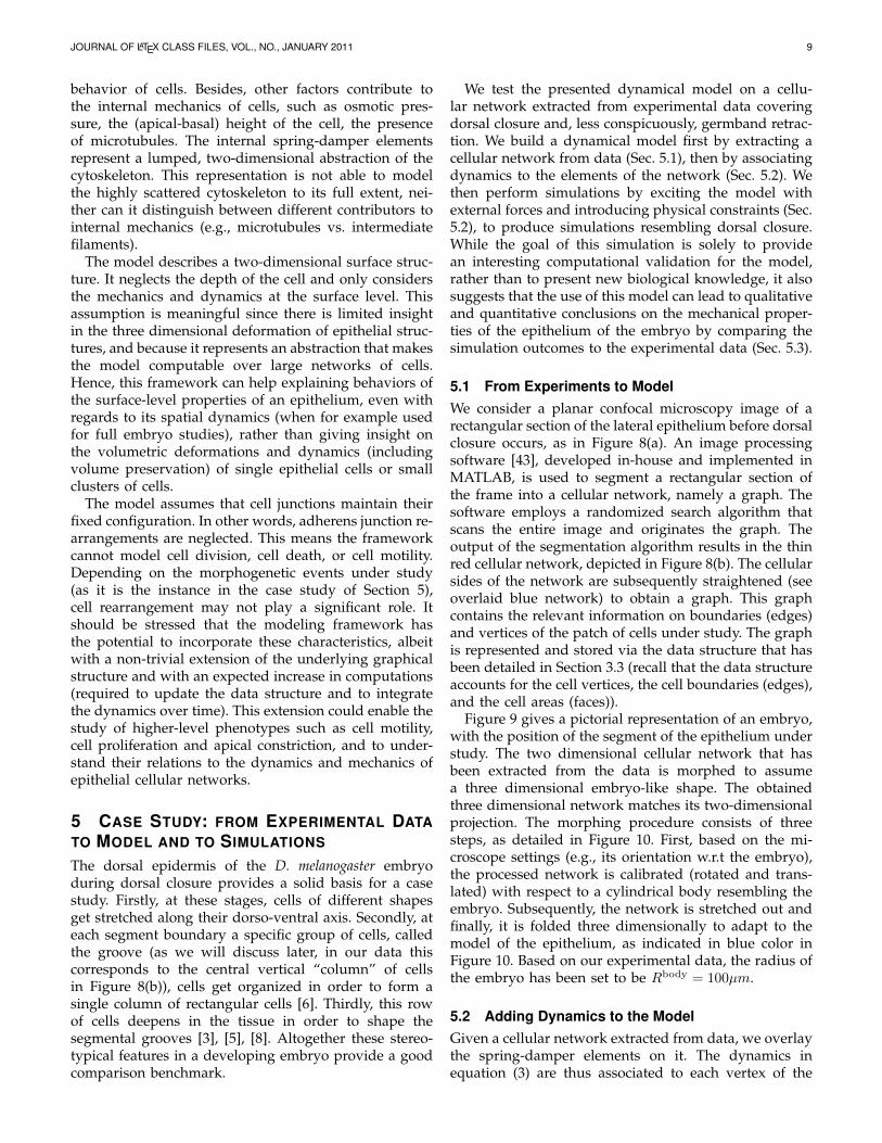
3.4 Dynamical Model: the Spring-Damper elementAssume that the underlying cellular geometry (that is,the underlying network topology) is known. A meshis overlaid to the cell junctions, that is to the pointswhere cell boundaries intersect (the magenta dots inFigure 5). A model is created as a two-dimensional, tiledsurface and is represented using the graph theoreticalnetwork notation given in Subsection 3.3. Within thisdata structure three different modeling elements (dis-cussed below) are discussed and associated to differentstructural features in epithelial cellular networks.
First, a magenta dot in Figure 5 represents a pointmass element mi associated to vertex vi, i ∈ {1, 2, . . . , N}.This models the inertia of the network via a constantmass value. However, let us importantly remark thatthe modeling approach is not intended to imply thatinertial forces are reflecting the underlying biology: theactual effect of the mass in the model dynamics can beeliminated by simple rescaling (as discussed later, wehave in practice used it to normalize the simulations timespan). The second law of Newton is applied to each pointmass element at vi by considering the global contributionall the forces ~Fi acting upon the point:
mi~xi(t) =∑i
~Fi(~x, t),
Fig. 5. A spring-damper model of a single cell. Discretepoints (large magenta dots) are adapted to the actualcell shape extracted from experiments (see Section 5.1).Black lines denote cell boundaries. Blue spring-damperelements are associated to boundaries, whereas greenones to intermediate pairs of non-adjacent points.
where ~xi(t) is the second time derivative of the position~xi of point mass mi, and ~x denotes a vector collecting allthe points ~xi. We will shortly express explicitly the forcecontribution in the equation above. The point masses areplaced at vertices, where different cell boundaries cometogether. It should be noted that in reality cell junctionsare not fixed, but they may rearrange with respect to theadjacent cell boundaries: the present modeling frame-work neglects these rearrangements. The implications ofthis assumption are further elaborated in Section 4.2.
The second element models the circumferential actinbelts, which organize along cell boundaries and connectadjacent cell vertices. Since these belts propagate theirelastic energy to adjacent components through thesevertices, a mechanistic equivalent will be used in themodel. The mechanical behavior of actin belts is visco-elastic and modeled by the presence of spring-damperelements (Voigt elements) between two adjacent cellvertices, as depicted in Figure 5 [37], [34]. Section 4.1discusses possible alternatives to the Voigt elements.In the following, these modules are called boundaryelements. A boundary element encompasses the belts oftwo adjacent cells, since these two cells are connectedthrough adherens junctions. Consider a point mass ele-ment mi connected to three other point mass elementsmj , j ∈ N (vi), where N (vi) denotes the set of verticesadjacent to vertex vi, as depicted in Figure 6. The pointmasses are connected through spring-damper elements,characterized respectively by stiffness coefficients ki,jand damping coefficients νi,j . The mathematical equa-tion for point mass element mi connected to the pointmasses mj via a spring-damper element, is given by:
mi~xi(t) = ~F elastici (~x) + ~F damping
i (~x) =∑j∈N (vi)
{(ki,j (li,j − di,j) + νi,j
dli,jdt
)~xj − ~xi||~xj − ~xi| |
},

JOURNAL OF LATEX CLASS FILES, VOL., NO., JANUARY 2011 7
kijvij
mi
mj
mj
mj
Fig. 6. A single point mass elementmi connected to threepoint mass elements (all denoted as mj) through spring-damper elements.
where li,j is the length of boundary element ei,j ,dli,jdt
is its time derivative, di,j is the resting length relatedto the spring at boundary element ei,j , and ~xj−~xi
||~xj−~xi|| isthe normalized vector accounting for orientation anddirection of the element ei,j .
As a third modeling element, the cytoskeleton (con-sisting of intermediate filaments and microtubules, seeFigure 1) is modeled similarly to the circumferentialactin belts using spring-damper elements, which in thefollowing will be denoted as intermediate elements. Withreference to the nodal characteristic of each single cell,elements are placed between all non-adjacent mass ele-ments within a cell, as depicted in green on Figure 5. Thecollection of intermediate elements represent a discreteabstraction of the cytoskeleton. Section 4.2 explains thepotential as well as the limitations of this approach. Themathematical equations for the elements are identical tothose of the external elements, that is
~F int.elastici (~x) + ~F int.damping
i (~x) =∑j∈N int(vi)
{(ki,j (li,j − di,j) + νi,j
dli,jdt
)~xj − ~xi||~xj − ~xi| |
},
where N int(vi) denotes the set of vertices laying withina face to which vertex vi belongs, but which are notdirectly adjacent to vi.
As anticipated in Section 2.1.3, the model considersnonlinear elasticity in cellular mechanics. The relation-ship between applied prestress and stiffness has a lin-ear characteristic, both on the cell [29] and on the cy-toskeletal component level [25]. To illustrate this relation,consider a spring, as depicted in Figure 7. The classicalconstitutive equation given by the Hooke law for themagnitude of the elastic force exerted by a spring is
F elastic(l) = k (l − d) , (1)
where k denotes the stiffness coefficient, l is the currentlength and d is the resting length of the spring. Prestressis defined as the fraction of the deviation from the restinglength, which is (l−d)
d . Now consider an affine relation
Fig. 7. One-dimensional spring model used to explain theapplied prestress.
between stiffness and applied prestress, as observed inexperiments [29]. This yields a coefficient
k(l).= k1
(l − d)
d+ k0, (2)
where k0 is the nominal (linear) stiffness coefficient atresting length and k1 accounts for the stiffness dueto applied prestress. Substituting the affine relation in(2) into equation (1) for the elastic force results in aquadratic (and thus nonlinear) elastic force-deformation(stress-strain) relation:
F elastic(l) = k(l) (l − d) =k1
2
(l − d)2
d+ k0 (l − d) .
The stiffness coefficients ki,j of the spring-damper ele-ments in the model are characterized according to thisnonlinear relation. This means that a pair of parame-ters (k0i,j/2, k
1i,j) is introduced for each spring-damper
element. Section 4.1 discusses possible extensions of theexpressions considered in (1)-(2).
In addition to the relations developed for the threemain modeling elements, the framework assumes thatthe connections between cells and the extracellular ma-trix are viscous. A friction force ~F friction
i is added, whichacts on each point mass element mi. ~F friction
i is inverselyproportional to the velocity ~xi of point mass mi,
~F frictioni (~xi) = −λi~xi,
where λi is the positive friction coefficient related topoint mass mi.
All the described components can be mathematicallyencompassed within a system of second-order ordinarydifferential equations (ODE). Formally, consider a pointmass mi at vertex vi representing 6 state variables, i.e.3 position variables ~xi and 3 velocity variables ~xi. Thedynamical ODE for mi is presented in (3) on page 8,where ki,j(·) and νi,j denote the stiffness and dampingcoefficients of an element between masses mi and mj ; li,jis the distance between the two masses; N (vi) denotesthe adjacent vertices of vi, and N int(vi) denotes thenon-adjacent vertices within all the neighboring facesof vi. The stiffness and damping forces can only act inthe direction of the element between the two masses,which is ~xj−~xi
||~xj−~xi|| . The parameter λi denotes the friction

JOURNAL OF LATEX CLASS FILES, VOL., NO., JANUARY 2011 8
mi~xi(t) = ~F elastici (~x) + ~F damping
i (~x) + ~F int.elastici (~x) + ~F int.damping
i (~x) + ~F frictioni (~xi) + ~F ex
i (~xi, t)
=∑
j∈N (vi)∪N int(vi)
{(ki,j(li,j) (li,j − di,j) + νi,j
dli,jdt
)~xj − ~xi||~xj − ~xi| |
}− λi~xi +
∑µ
~F ex,µi (~xi, t) (3)
coefficient at mass mi, whereas∑µ~F ex,µi denotes the
sum of all possible external, time-dependent forces µacting on mass mi. (In Section 5.2 we shall consider afew examples for external forces and show that theyalso enable the embedding of spatial constraints in themodel.)
The model in (3) is nonlinear, due to the presenceof the lengths li,j and their time derivatives, and be-cause of the varying stiffness coefficients ki,j(li,j). Amatrix formulation can be derived using the LaplacianL defined above. First introduce a matrix S based on(3), which structure is related to that of L: notice that‖~xj − ~xi‖ = li,j , and define the non-diagonal entries(i 6= j) of S as
sij = −(ki,j(li,j) (li,j − di,j) + νi,j
dli,jdt
)1
||~xj−~xi||
= −(ki,j(li,j)
li,j−di,jli,j
+νi,jli,j
dli,jdt
),
and similarly the diagonal entries as
sii =∑
j∈N (vi)∪N int(vi)
{ki,j(li,j)
li,j − di,jli,j
+νi,jli,j
dli,jdt
}.
Subsequently, S can be exploited to rewrite the dynam-ical equations in (3) for the whole network of pointmasses in matrix notation as follows: ~x
−~x
(t) =
[O I
M−1S(k, l, t) −M−1Λ
] ~x−~x
(t)
+
0
M−1∑µ F
ex,µ(~x, t)
, (4)
where M is a 3N ×3N diagonal matrix composed of themasses mi, and Λ is a 3N×3N diagonal matrix with thefriction coefficients λi. S is time-dependent and containsall the nonlinearities of the equations. The values ofki,j(·), li,j , and dli,j/dt need to be updated in time for allspring-damper elements: the Laplacian L can be used toassign the updated variables to the corresponding entriesin S. Using smart vectorial implementations in MATLAB,the simulation algorithm can integrate the dynamics in(4) of a mass spring-damper network with dimensions inthe order of hundreds of vertices in a computationallyrapid way. The simulation can also benefit from tech-niques developed in the computer graphics community,for the development of simulators of soft-body dynamics[39]. We shall further discuss computational issues of themodel in Section 5.2.
4 DISCUSSION ON THE MODEL
The presented modeling framework incorporates bothbiological insight and engineering principles. Based onthis modeling framework, the dynamical equations canbe extended by introducing terms that account for newknowledge gained from both experiments and simula-tions. On the other hand, the choices made on the modelarchitecture also pose limitations over its general appli-cation. We discuss next both potential and the limitationsof the model.
4.1 Potential: model extensions and applications
The dynamical model allows to embed the effect ofgeneral, time-varying, non-linear, external forces. Withreference to Figure 3 and the related discussion onnonlinearity of cellular elasticity, it is possible to in-clude hysteresis and memory effects in the stress/straincharacteristic by direct modification of Equation (2): thefirst feature can be useful to prevent dynamical high-frequency oscillations that are usually not observed ex-perimentally, whereas the second can lead to the mod-eling of permanent cellular deformations. However, thiscan lead to higher computational costs. The choice ofviscoelastic Voigt modules as interconnections betweencellular junctions has been motivated by literature evi-dence and model testing, but can be as well substitutedby Maxwell elements or – at the expense of an increase incomplexity – by standard-linear or generalized-Maxwellelements [30]. The model also allows for the introductionof physical and spatial constraints, as will be discussedin the case study of Section 5.
The presence of an underlying dynamical model al-lows generating simulation outputs that can be matchedto time-lapse experiments. This may help to explainmechanical properties of the network, for instance byidentifying its stiffness parameters or friction coeffi-cients. There are a number of advanced parameter iden-tification techniques that could be used with this goal[40], [41], [42]. The model can furthermore help quan-titatively studying certain morphogenetic effects suchas germband retraction, groove formation, or dorsalclosure. At the cell level, the study of elastic propertiesvia laser ablation experiments can also represent an in-teresting potential to test the model on, where generateddata would be matched to the model simulations.
4.2 Limitations
The cytoskeleton, scattered throughout the whole cell(cf. Subsection 2.1.1), influences most of the mechanical
JOURNAL OF LATEX CLASS FILES, VOL., NO., JANUARY 2011 9
behavior of cells. Besides, other factors contribute tothe internal mechanics of cells, such as osmotic pres-sure, the (apical-basal) height of the cell, the presenceof microtubules. The internal spring-damper elementsrepresent a lumped, two-dimensional abstraction of thecytoskeleton. This representation is not able to modelthe highly scattered cytoskeleton to its full extent, nei-ther can it distinguish between different contributors tointernal mechanics (e.g., microtubules vs. intermediatefilaments).
The model describes a two-dimensional surface struc-ture. It neglects the depth of the cell and only considersthe mechanics and dynamics at the surface level. Thisassumption is meaningful since there is limited insightin the three dimensional deformation of epithelial struc-tures, and because it represents an abstraction that makesthe model computable over large networks of cells.Hence, this framework can help explaining behaviors ofthe surface-level properties of an epithelium, even withregards to its spatial dynamics (when for example usedfor full embryo studies), rather than giving insight onthe volumetric deformations and dynamics (includingvolume preservation) of single epithelial cells or smallclusters of cells.
The model assumes that cell junctions maintain theirfixed configuration. In other words, adherens junction re-arrangements are neglected. This means the frameworkcannot model cell division, cell death, or cell motility.Depending on the morphogenetic events under study(as it is the instance in the case study of Section 5),cell rearrangement may not play a significant role. Itshould be stressed that the modeling framework hasthe potential to incorporate these characteristics, albeitwith a non-trivial extension of the underlying graphicalstructure and with an expected increase in computations(required to update the data structure and to integratethe dynamics over time). This extension could enable thestudy of higher-level phenotypes such as cell motility,cell proliferation and apical constriction, and to under-stand their relations to the dynamics and mechanics ofepithelial cellular networks.
5 CASE STUDY: FROM EXPERIMENTAL DATATO MODEL AND TO SIMULATIONS
The dorsal epidermis of the D. melanogaster embryoduring dorsal closure provides a solid basis for a casestudy. Firstly, at these stages, cells of different shapesget stretched along their dorso-ventral axis. Secondly, ateach segment boundary a specific group of cells, calledthe groove (as we will discuss later, in our data thiscorresponds to the central vertical “column” of cellsin Figure 8(b)), cells get organized in order to form asingle column of rectangular cells [6]. Thirdly, this rowof cells deepens in the tissue in order to shape thesegmental grooves [3], [5], [8]. Altogether these stereo-typical features in a developing embryo provide a goodcomparison benchmark.
We test the presented dynamical model on a cellu-lar network extracted from experimental data coveringdorsal closure and, less conspicuously, germband retrac-tion. We build a dynamical model first by extracting acellular network from data (Sec. 5.1), then by associatingdynamics to the elements of the network (Sec. 5.2). Wethen perform simulations by exciting the model withexternal forces and introducing physical constraints (Sec.5.2), to produce simulations resembling dorsal closure.While the goal of this simulation is solely to providean interesting computational validation for the model,rather than to present new biological knowledge, it alsosuggests that the use of this model can lead to qualitativeand quantitative conclusions on the mechanical proper-ties of the epithelium of the embryo by comparing thesimulation outcomes to the experimental data (Sec. 5.3).
5.1 From Experiments to ModelWe consider a planar confocal microscopy image of arectangular section of the lateral epithelium before dorsalclosure occurs, as in Figure 8(a). An image processingsoftware [43], developed in-house and implemented inMATLAB, is used to segment a rectangular section ofthe frame into a cellular network, namely a graph. Thesoftware employs a randomized search algorithm thatscans the entire image and originates the graph. Theoutput of the segmentation algorithm results in the thinred cellular network, depicted in Figure 8(b). The cellularsides of the network are subsequently straightened (seeoverlaid blue network) to obtain a graph. This graphcontains the relevant information on boundaries (edges)and vertices of the patch of cells under study. The graphis represented and stored via the data structure that hasbeen detailed in Section 3.3 (recall that the data structureaccounts for the cell vertices, the cell boundaries (edges),and the cell areas (faces)).
Figure 9 gives a pictorial representation of an embryo,with the position of the segment of the epithelium understudy. The two dimensional cellular network that hasbeen extracted from the data is morphed to assumea three dimensional embryo-like shape. The obtainedthree dimensional network matches its two-dimensionalprojection. The morphing procedure consists of threesteps, as detailed in Figure 10. First, based on the mi-croscope settings (e.g., its orientation w.r.t the embryo),the processed network is calibrated (rotated and trans-lated) with respect to a cylindrical body resembling theembryo. Subsequently, the network is stretched out andfinally, it is folded three dimensionally to adapt to themodel of the epithelium, as indicated in blue color inFigure 10. Based on our experimental data, the radius ofthe embryo has been set to be Rbody = 100µm.
5.2 Adding Dynamics to the ModelGiven a cellular network extracted from data, we overlaythe spring-damper elements on it. The dynamics inequation (3) are thus associated to each vertex of the

JOURNAL OF LATEX CLASS FILES, VOL., NO., JANUARY 2011 10
(a) Confocal microscopy image. The red polygon indicates the subnet-work of interest.
(b) A processed version of the network. The thin red graphis the raw processed network, whereas the straight thick bluelines constitute the graph to be used in the simulations.
Fig. 8. Isolated cellular network at starting time, used formodel building.
y
x
z
dorsal
ventral
anterior(head)
posterior(tail)
y
x
z
dorsal
ventral
anterior(head)
posterior(tail)
amnioserosa
epithelium
amnioserosa
epithelium
Fig. 9. Pictorial model of the embryo, depicting a segmentof the epithelium (blue). The dorsal closure forces actingon the epithelium over the amnioserosa (pink region) areindicated by the blue arrows.
stored cellular network and allow for the inclusion ofexternal forces. The model in equation (3) depends on aset of parameters, which characterize spring and damperelements (both boundary and internal ones, both forstiffness and resting prestress), friction in the model,as well as external forces and constraints (the latterwill be discussed shortly). These parameters need to beinstantiated according to the data and to the goal of the
calibrated 2D projection
2D back projection
3D model, folded on cylinder
embryo
z
y
01 2 3
xz
y
Fig. 10. Top: A pictorial longitudinal view of the embryowith indication of calibration, back projection, and foldingsteps, which together yield the folded, three-dimensionalmodel of the epithelium. Bottom: A three-dimensionalview of the morphing procedure.
simulation. In this study, their value is selected froma set of simulation tests, each of which is driven by aspecific external force. The goal of these tests is, given aspecific cellular network and a set of forces, to produceoutputs that are qualitatively acceptable, namely thatdo not present unstable, unrealistic, on non-physicaldynamics. Notice from Equation (3) that there is a linearrelationship between the time horizon of a simulationand the value of the mass. We have thus decided torescale both in order to normalize the first to span theunit interval.
One important set of forces that acts on epidermalcells comes from the developing central nervous system(CNS). The ventral epithelium closely wraps around theCNS, thus the epithelium experiences the CNS as aphysical constraint. While the precise mechanical char-acteristics of the CNS have not been investigated, it isobserved that folds rarely appear in the epidermis jux-taposed to the CNS. Only strong grooves, generated ingenetic over-expression experiments, partially pinch intothe CNS. This observation suggests that in general theCNS is able to resist pressure exerted by the overlayingepidermis. In our model the CNS is abstracted as twoadjacent and parallel cylinders, as in Figure 11. Theradius of each cylinder of the CNS, RCNS is estimatedfrom cross section experiments to be one fifth of theradius of the embryo Rbody. Ideally the CNS only actson mass elements that are in contact with it. However,modeling the CNS as a hard physical constraint maybe both biologically unrealistic (organs are not infinitely
JOURNAL OF LATEX CLASS FILES, VOL., NO., JANUARY 2011 11
rigid) and practically undesired (it may lead to stiffdynamics). Inspired by an approach developed in thecomputer graphics community for the development ofsimulators of soft-body dynamics [39], the interactionbetween embryo and CNS is implemented as an externalforce acting on the epithelium along a direction that isnormal to the CNS cylinder. Let us denote the distancevector from the axis of the CNS to a vertex i by ~ri. Ourimplementation employs a polynomial formulation thatdepends on a parameter u ∈ N:
~FCNSi (~ri) =
{ (||~ri||−2RCNS
RCNS
)2u~ri||~ri|| , for ||~ri| | < 2RCNS
0 , otherwise.
The interaction of the epithelium with the CNS can betuned and stiff dynamics can be avoided.
0
50
100
150
−80−60
−40−20
020
4060
80
−80
−60
−40
−20
0
20
40
xz
y
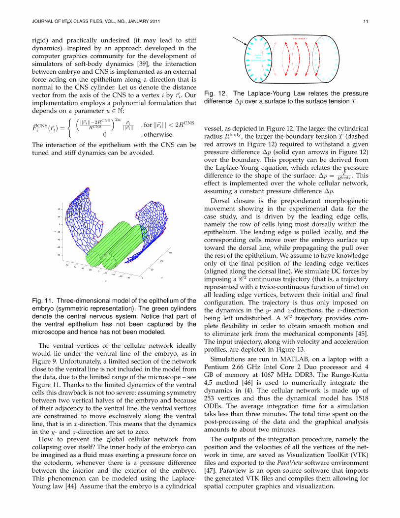
Fig. 11. Three-dimensional model of the epithelium of theembryo (symmetric representation). The green cylindersdenote the central nervous system. Notice that part ofthe ventral epithelium has not been captured by themicroscope and hence has not been modeled.
The ventral vertices of the cellular network ideallywould lie under the ventral line of the embryo, as inFigure 9. Unfortunately, a limited section of the networkclose to the ventral line is not included in the model fromthe data, due to the limited range of the microscope – seeFigure 11. Thanks to the limited dynamics of the ventralcells this drawback is not too severe: assuming symmetrybetween two vertical halves of the embryo and becauseof their adjacency to the ventral line, the ventral verticesare constrained to move exclusively along the ventralline, that is in x-direction. This means that the dynamicsin the y- and z-direction are set to zero.
How to prevent the global cellular network fromcollapsing over itself? The inner body of the embryo canbe imagined as a fluid mass exerting a pressure force onthe ectoderm, whenever there is a pressure differencebetween the interior and the exterior of the embryo.This phenomenon can be modeled using the Laplace-Young law [44]. Assume that the embryo is a cylindrical
wall tension T
reactionforce
(pressure p)
Fig. 12. The Laplace-Young Law relates the pressuredifference ∆p over a surface to the surface tension T .
vessel, as depicted in Figure 12. The larger the cylindricalradius Rbody, the larger the boundary tension T (dashedred arrows in Figure 12) required to withstand a givenpressure difference ∆p (solid cyan arrows in Figure 12)over the boundary. This property can be derived fromthe Laplace-Young equation, which relates the pressuredifference to the shape of the surface: ∆p = T
Rbody . Thiseffect is implemented over the whole cellular network,assuming a constant pressure difference ∆p.
Dorsal closure is the preponderant morphogeneticmovement showing in the experimental data for thecase study, and is driven by the leading edge cells,namely the row of cells lying most dorsally within theepithelium. The leading edge is pulled locally, and thecorresponding cells move over the embryo surface uptoward the dorsal line, while propagating the pull overthe rest of the epithelium. We assume to have knowledgeonly of the final position of the leading edge vertices(aligned along the dorsal line). We simulate DC forces byimposing a C 2 continuous trajectory (that is, a trajectoryrepresented with a twice-continuous function of time) onall leading edge vertices, between their initial and finalconfiguration. The trajectory is thus only imposed onthe dynamics in the y- and z-directions, the x-directionbeing left undisturbed. A C 2 trajectory provides com-plete flexibility in order to obtain smooth motion andto eliminate jerk from the mechanical components [45].The input trajectory, along with velocity and accelerationprofiles, are depicted in Figure 13.
Simulations are run in MATLAB, on a laptop with aPentium 2.66 GHz Intel Core 2 Duo processor and 4GB of memory at 1067 MHz DDR3. The Runge-Kutta4,5 method [46] is used to numerically integrate thedynamics in (4). The cellular network is made up of253 vertices and thus the dynamical model has 1518ODEs. The average integration time for a simulationtaks less than three minutes. The total time spent on thepost-processing of the data and the graphical analysisamounts to about two minutes.
The outputs of the integration procedure, namely theposition and the velocities of all the vertices of the net-work in time, are saved as Visualization ToolKit (VTK)files and exported to the ParaView software environment[47]. Paraview is an open-source software that importsthe generated VTK files and compiles them allowing forspatial computer graphics and visualization.

JOURNAL OF LATEX CLASS FILES, VOL., NO., JANUARY 2011 12
0 0.1 0.2 0.3 0.4 0.5 0.6 0.7 0.8 0.9 10
0.5
1C2 displacement profi le
t
pL
E(t
)
0 0.1 0.2 0.3 0.4 0.5 0.6 0.7 0.8 0.9 10
1
2
t
vL
E(t
)
0 0.1 0.2 0.3 0.4 0.5 0.6 0.7 0.8 0.9 1−10
0
10
t
aL
E(t
)
Fig. 13. C 2 trajectory imposed on the leading edgevertices. Top down displacement profile pLE(t), velocityprofile vLE(t), and acceleration profile aLE(t). The timeaxis has been normalized.
5.3 Simulations
We select a stiffness coefficient k0 for the central verticalcolumn of cells in Figure 8(b) that is twice as highas that of the remaining cells. These cells display anaccumulation of cytoskeletal proteins compared to theirnon-groove neighbors [6]. This is the case for instance forEnabled, which is implicated in the organization of actinfilaments [48], as well as the beta-catenin Armadillo,which links the adherens junctions to the cytoskeleton[49]. Higher stiffness of these specific cells is related tothe emergence of grooves, a phenomenon we are notgoing to further focus on.
We expect the cells to stretch vertically and showalignment, particularly around the mid column of Figure8(b). We are thus interested in quantitatively assessingthe quality of the simulations with respect
2) to the alignment of cells, and3) to their elongation.This outcome may indicate that the accumulation of
cytoskeletal components in the groove cells is consistentwith a different behavior of these cells at the mechanicallevel and may be responsible for their rectangular shape.This possibility will need to be addressed with genetictools in vivo. Therefore, this contribution has no explicitgoal to shed new light over the biological data underconsideration: we are instead interested to qualitativelyshow that simulations of the model, which has beeninitialized to fit the data, can reproduce the behaviorobserved in experiments. This indicates the possiblegeneral use of the proposed modeling framework insimilar studies.
5.3.1 Qualitative analysis of the simulation scenarios
Figure 14 displays the rendered outputs of a singlesimulation. They are to be compared with the image inFigure 15(a), representing the network of cells in Figure8(a) at a later stage, after dorsal closure has ensued.
(a) Dorsal view (b) 3D view
(c) Lateral view (d) Longitudinal view
Fig. 14. Three-dimensional simulation outcomes. Thecartesian axes are x (red), y (yellow), and z (green).
Notice that the indenting central column approachesthe CNS cylinder and interacts with it, which calls forthe use of the corresponding external forces discussedearlier. The dorsal and lateral view clearly indicate thatcell boundaries line up along columns in dorso-ventraldirection. In particular, the central column lines up in analmost perfect ladder configuration. It is also quite clearthat cells stretch in the vertical direction. A limitationof the simulations is visible on the leading edge which,unlike in the experimental image, is nicely aligned:this artificial effect is due to the imposed simulationdynamics (input trajectory) over the leading edge andcan be possibly eliminated by feeding to the simulationa more realistic trajectory for those specific cells.
5.3.2 Quantitative analysis of the simulation scenariosWe now consider the processed cellular network inFigure 15(b), which is extracted from the experimentaldata in Figure 15(a). It clearly relates to the networkin Figure 8(b), except for a few extra cells that havebeen caught by the microscope and appear close to the
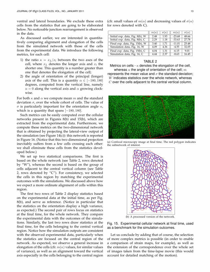
JOURNAL OF LATEX CLASS FILES, VOL., NO., JANUARY 2011 13
ventral and lateral boundaries. We exclude these extracells from the statistics that are going to be elaboratedbelow. No noticeable junction rearrangement is observedin the data.
As discussed earlier, we are interested in quantita-tively comparing alignment and elongation of the cellsfrom the simulated network with those of the cellsfrom the experimental data. We introduce the followingmetrics, for each cell:
1) the ratio κ = xL/xl between the two axes of thecell, where xL denotes the longer axis and xl theshorter one. This quantity is a number greater thanone that denotes the elongation of the cell;
2) the angle of orientation of the principal (longer)axis of the cell. This is a quantity α ∈ [−180, 180]degrees, computed from the vertical line, namelyα = 0 along the vertical axis and α growing clock-wise.
For both κ and α we compute mean m and the standarddeviation σ, over the whole cohort of cells. The value ofσ is particularly important for the orientation angle α,which is a quantity that spans [−180, 180].
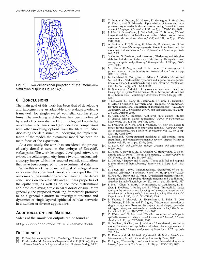
Such metrics can be easily computed over the cellularnetworks present in Figures 8(b) and 15(b), which areextracted from the experimental data. Furthermore, wecompute these metrics on the two-dimensional networkthat is obtained by projecting the lateral-view output ofthe simulation (see Figure 14(c)): this network is reportedin Figure 16. (Notice that this two dimensional projectioninevitably suffers from a few cells crossing each other:we shall eliminate these cells from the statistics devel-oped below.)
We set up two statistical comparisons. The first isbased on the whole network (see Table 2, rows denotedby “W”), whereas the second is based on the group ofcells adjacent to the central vertical column (see Table2, rows denoted by “C”). For consistency, we selectedthe cells in this region by matching the experimentaloutcomes with the simulations. We discussed above howwe expect a more ordinate alignment of cells within thisregion.
The first two rows of Table 2 display statistics basedon the experimental data at the initial time, as per Fig.8(b), and serve as reference. (Notice in particular thatthe statistics on the orientation display a high variance,as expected.) The second pair of rows focus on statisticsat the final time, for the whole network. They comparethe experimental data with the outcomes of the simula-tions. Similarly, the last two rows draw statistics at thefinal time, for the cells belonging to the central verticalregion. Notice how the simulation outputs are consistentwith the observed experimental data, particularly whenthe statistics are focused on the central region of thenetwork. As expected, we observe a general increase inelongation of the cells (cfr. m(κ) values, for similar valuesof variance), as well as an alignment toward the verticalaxis especially in the cells belonging to the central region
(cfr. small values of m(α) and decreasing values of σ(α)for rows denoted with C).
m(κ) σ(κ) m(α) σ(α)
Initial exp. data, Fig. 8(b), W 2.48 1.93 -23.68 48.66Initial exp. data, Fig. 8(b), C 2.29 1.18 -33.63 27.78Final exp. data, Fig. 15(b), W 3.40 1.71 -11.01 25.48Simulation data, Fig. 16, W 4.09 4.36 -4.55 32.05Final exp. data, Fig. 15(b), C 4.04 1.31 -6.15 9.01Simulation data, Fig. 16, C 4.44 2.37 -8.63 16.45
TABLE 2Metrics on cells - κ denotes the elongation of the cell,
whereas α the angle of orientation of the cell; mrepresents the mean value and σ the standard deviation;W indicates statistics over the whole network, whereasC over the cells adjacent to the central vertical column.
(a) Confocal microscopy image at final time. The red polygon indicatesthe subnetwork of interest.
!!"" " !"" #"" $"" %""
!&""
!%&"
!%""
!$&"
!$""
!#&"
!#""
!!&"
!!""
!&"
(b) A processed version of the network.
Fig. 15. Experimental cellular network at final time, usedas a benchmark for the simulation outcomes.
Let us conclude by adding that of course, the selectionof more complex metrics is possible (in order to enablea comparison of strain maps, for example), as well asthe extension of the correspondence over the whole setof images taken from the time-lapse movie (this wouldaccount for detailed matching of the motion).
JOURNAL OF LATEX CLASS FILES, VOL., NO., JANUARY 2011 14
0 50 100 150 200 250 3000
50
100
150
200
250
300
350
400
Fig. 16. Two dimensional projection of the lateral-viewsimulation output in Figure 14(c).
6 CONCLUSIONS
The main goal of this work has been that of developingand implementing an adaptable and scalable modelingframework for single-layered epithelial cellular struc-tures. The modeling architecture has been motivatedby a set of criteria distilled from biological knowledgeon cellular mechanics, and grounded on comparisonswith other modeling options from the literature. Afterdiscussing the data structure underlying the implemen-tation of the model, the dynamical model has been themain focus of the exposition.
As a case study, the work has considered the processof early dorsal closure on the embryo of Drosophilamelanogaster. The work leveraged developed software toextract the cellular geometry from a two-dimensional mi-croscopy image, which has enabled realistic simulationsthat have been compared to the experimental data.
While this work has no explicit goal of biological rele-vance over the considered case study, we expect that theoutcomes of the simulations can be meaningful to deriveconclusions on the elasticity and stiffness properties ofthe epithelium, as well as on the force distributionsand profiles playing a role in early dorsal closure. Moregenerally, the proposed modeling framework promisesto be a general platform to investigate structure anddynamics of single-layered epithelial cellular networksin a number of diverse applications.
ADDITIONAL ON-LINE MATERIAL
Videos of the simulation outputs can be found at:
http://www.dcsc.tudelft.nl/∼aabate/tcbb
REFERENCES
[1] D. Boal, Mechanics of the Cell. Cambridge University Press, 2011.[2] R. Alexander, M. Anderson, Chaplain, and K. R. (Editors), Single-
cell-based Models in Biology and Medicine. Springer Verlag, 2007.
[3] X. Peralta, Y. Toyama, M. Hutson, R. Montague, S. Venakides,D. Kiehart, and G. Edwards, “Upregulation of forces and mor-phogenic asymmetries in dorsal closure during Drosophila devel-opment,” Biophysical Journal, vol. 92, no. 7, pp. 2583–2596, 2007.
[4] J. Solon, A. Kaya-Copur, J. Colombelli, and D. Brunner, “Pulsedforces timed by a ratchet-like mechanism drive directed tissuemovement during dorsal closure,” Cell, vol. 137, no. 7, pp. 1331–1342, 2009.
[5] A. Layton, Y. T. Y, G. Yang, G. Edwards, D. Kiehart, and S. Ve-nakides, “Drosophila morphogenesis: tissue force laws and themodeling of dorsal closure,” HFSP Journal, vol. 3, no. 6, pp. 441–460, 2009.
[6] S. Vincent, N. Perrimon, and J. Axelrod, “Hedgehog and Winglessstabilize but do not induce cell fate during Drosophila dorsalembryonic epidermal patterning,” Development, vol. 135, pp. 2767–2775, 2008.
[7] M. Gibson, R. Nagpal, and N. Perrimon, “The emergence ofgeometric order in proliferating metazoan epithelia,” Nature, pp.1038–1041, 2006.
[8] G. Blanchard, S. Murugesu, R. Adams, A. Martinez-Arias, andN. Gorfinkiel, “Cytoskeletal dynamics and supracellular organisa-tion of cell shape fluctuations during dorsal closure,” Development,vol. 137, no. 16, pp. 2743–2752, 2010.
[9] D. Stamenovic, “Models of cytoskeletal mechanics based ontensegrity,” in Cytoskeletal Mechanics, M. R. Kazempur-Mofrad andR. D. Kamm, Eds. Cambridge University Press, 2006, pp. 103 –128.
[10] T. Cickovski, C. Huang, R. Chaturvedi, T. Glimm, H. Hentschel,M. Alber, J. Glazier, S. Newman, and J. Izaguirre, “A frameworkfor three-dimensional simulation of morphogenesis,” IEEE/ACMTransactions on Computational Biology and Bioinformatics, vol. 2, pp.273–288, October 2005.
[11] H. Chen and G. Brodland, “Cell-level finite element studiesof viscous cells in planar aggregates,” Journal of BiomechanicalEngineering, vol. 122, pp. 394–401, 2000.
[12] G. Brodland, D. Viens, and J. Veldhuis, “A new cell-based femodel for the mechanics of embryonic epithelia,” Computer Meth-ods in Biomechanics and Biomedical Engineering, vol. 10, no. 2, pp.121–128, April 2007.
[13] G. Brodland, “Computational modeling of cell sorting, tissueengulfment, and related phenomena: A review,” Applied MechanicsReview, vol. 57, no. 1, pp. 47–76, 2004.
[14] G. Karp, Cell and Molecular Biology: Concepts and Experiments.Wiley, 2004.
[15] K. Kasza, A. Rowat, J. Liu, T. Angelini, C. Brangwynne, G. Koen-derink, and D. Weitz, “The cell as a material,” Current Opinion inCell Biology, vol. 19, pp. 101–107, 2007.
[16] D. Discher, P. Janmey, and Y. Wang, “Tissue cells feel and respondto the stiffness of their substrate,” Science, vol. 310, pp. 1139–1143,2005.
[17] D. Pesen and J. Hoh, “Micromechanical architecture of the en-dothelial cell cortex,” Biophysical Journal, vol. 88, pp. 670–679, 2005.
[18] U. Potard, J. Butler, and N. Wang, “Cytoskeletal mechanics in con-fluent epithelial cells probed through integrins and e-cadherins,”American Journal of Physiology, vol. 272, no. 41, pp. 1654–1663, 1997.
[19] S. Hu, J. Chen, B. Fabry, Y. Numaguchi, A. Gouldstone, D. In-gber, J. Fredberg, J. Butler, and N. Wang, “Intracellular stresstomography reveals stress focusing and structural anisotropy incytoskeleton of living cells,” American Journal of Physiology CellPhysiology, vol. 285, pp. C1082–C1090, 2003.
[20] S. Kumar, I. Maxwell, A. Heisterkamp, T. Polte, T. Lele,M. Salanga, E. Mazur, and D. Ingber, “Viscoelastic retraction ofsingle living stress fibers and its impact on cell shape, cytoskele-tal organization, and extracellular matrix mechanics,” BiophysicalJournal, vol. 90, pp. 3762–3773, May 2006.
[21] C. Wiebe and G. Brodland, “Tensile properties of embryonicepithelia measured using a novel instrument,” Journal of Biome-chanics, vol. 38, pp. 2087–2094, 2005.
[22] G. Brodland, D. Chen, and J. Veldhuis, “A cell-based constitutivemodel for embryonic epithelia and other planar aggregates ofbiological cells,” International Journal of Plasticity, vol. 22, pp. 965–995, 2006.
[23] R. Kamm and M. Mofrad, Cytoskeletal Mechanics: Models andMeasurements, 1st ed. Cambridge University Press, 2006.
[24] D. Ingber, “Tensegrity I. cell structure and hierarchical systemsbiology,” Journal of Cell Science, vol. 116, pp. 1157–1173, 2003.
JOURNAL OF LATEX CLASS FILES, VOL., NO., JANUARY 2011 15
[25] D. Stamenovic, M. Mijailovich, I. Tolic-Nørrelykke, J. Chen, andN. Wang, “Cell prestress. II. Contribution of microtubules,” Amer-ican Journal of Physiology, vol. 282, pp. 617–624, 2002.
[26] X. Chen and G. Brodland, “Mechanical determinants of epithe-lium thickness in early-stage embryos,” Journal of MechanicalBehavior of Biomedical Materials, vol. 2, pp. 494–501, 2009.
[27] R. Zaidel-Bar, M. Cohen, L. Addadi, and B. Geiger, “Hierarchicalassembly of cell–matrix adhesion complexes,” Biochemical SocietyTransactions, vol. 32, no. 3, pp. 416–420, 2004.
[28] F. Beer, E. Johnston, J. Dewolf, and D. Mazurek, Mechanics of theCell. McGraw Hil, 2009.
[29] N. Wang, I. Tolic-Nørrelykke, J. Chen, S. Mijailovich, J. Butler,J. Fredberg, and D. Stamenovic, “Cell prestress. I. Stiffness andprestress are closely associated in adherent contractile cells,”American Journal of Physiology, vol. 282, pp. 606–616, 2002.
[30] Y. Fung, Biomechanics: Mechanical Properties of Living Tissues,2nd ed. Springer-Verlag, 1993.
[31] V. Vasioukhin and E. Fuchs, “Actin dynamics and cell-cell ad-hesion in epithelia,” Current Opinion in Cell Biology, vol. 13, pp.76–84, 2001.
[32] Y. Luo, X. Xu, T. Lele, S. Kumar, and D. Ingber, “A multi-modulartensegrity model of an actin stress fiber,” Journal of Biomechanics,vol. 41, pp. 2379–2387, 2008.
[33] A. Munjiza, The Combined Finite-Discrete Element Method. Wiley,2004.
[34] W. Mollemans, F. Schutyser, J. Van Cleynenbreugel, andP. Suetens, “Tetrahedral mass spring model for fast soft tissuedeformation,” in Surgery Simulation and Soft Tissue Modeling,N. Ayache and H. Delingette, Eds. Springer-Verlag, 2003, vol.2673, pp. 145–154.
[35] G. Odell, G. Oster, B. Burnside, and P. Alberch, “A mechanicalmodel for epithelial morphogenesis,” Journal of Mathematical Biol-ogy, vol. 9, pp. 291–295, 1980.
[36] D. Terzopoulos and K. Waters, “Physically-based facial modeling,analysis, and animation,” Journal of Visualization and ComputerAnimation, vol. 1, no. 2, pp. 73–80, 1990.
[37] L. Cooper and S. Maddock, “Preventing collapse within mass-spring-damper models of deformable objects,” in Proceedings of theFifth International Conference in Central Europe on Computer Graphicsand Visualization, Plzn, Czech Republic, 1997, pp. 196–204.
[38] M. Arcak and E. Sontag, “A passivity-based stability criterion fora class of biochemical reaction networks,” Journal of MathematicalBiosciences and Engineering, vol. 5, no. 1, pp. 1–19, 2008.
[39] A. Nealen, M. Muller, R. Keiser, E. Boxerman, and M. Carlson,“Physically based deformable models in computer graphics,”Computer Graphics Forum, vol. 25, no. 4, pp. 809–836, 2005.
[40] D. Chen and B. Paden, “Stable inversion of nonlinear non-minimum phase systems,” International Journal of Control, vol. 64,no. 1, pp. 81–97, 1996.
[41] S. Devasia and B. Paden, “Stable inversion for nonlinearnonminimum-phase time-varying systems,” IEEE Transactions onAutomatic Control, vol. 43, no. 2, pp. 283–288, 1998.
[42] R. Raffard, K. Amondlirdviman, J. Axelrod, and C. Tomlin, “Anadjoint-based parameter identification algorithm applied to pla-nar cell polarity signaling,” IEEE Transactions on Automatic Control,vol. 53, pp. 109–121, 2008.
[43] A. Silletti, A. Cenedese, and A. Abate, “The emergent structure ofthe Drosophila Wing - a dynamic model generator,” in Proceedingsof the International Conference on Computer Vision, Theory and Appli-cations (VISAPP 09), Lisboa, Portugal, February 2009, pp. 406–410.
[44] R. Phillips, J. Kondev, and J. Theriot, Physical Biology of the Cell,1st ed. Garland Science, 2009.
[45] L. Tsai, Robot analysis: the mechanics of serial and parallel manipula-tors. Wiley & Sons, 1999.
[46] J. Dormand and P. Prince, “A family of embedded Runge-Kuttaformulae,” Journal of Computational Applied Mathematics, vol. 6, pp.19–26, 1980.
[47] J. Ahrens, B. Geveci, and C. Law, “ParaView: An end-user tool forlarge data visualization,” in The Visualization Handbook, C. Hansenand C. Johnson, Eds. Elsevier, 2005.
[48] A. Kiger, B. Baum, S. Jones, M. Jones, A. Coulson, C. Echeverri,and N. Perrimon, “A functional genomic analysis of cell morphol-ogy using RNA interference,” Journal of Biology, vol. 2, no. 4, p. 27,2003.
[49] M. Peifer, “The product of the Drosophila segment polarity genearmadillo is part of a multi-protein complex resembling the
vertebrate adherens junction,” Journal of cell science, vol. 105, no. 4,pp. 993–1000, 1993.
Alessandro Abate received a Laurea in Electri-cal Engineering in October 2002 from the Uni-versity of Padova (Italy), an MS in May 2004and a PhD in December 2007, both in Electri-cal Engineering and Computer Sciences, at UCBerkeley. He has been an International Fellow inthe CS Lab at SRI International in Menlo Park(CA), and a PostDoctoral Researcher at Stan-ford University, in the Department of Aeronauticsand Astronautics. Since June 2009, he has beenan Assistant Professor at the Delft Center for
Systems and Control (DCSC), TU Delft - Delft University of Technology.His research interests are in the analysis, verification, and control ofprobabilistic and hybrid systems, and in their general application over anumber of domains, particularly in systems biology.
Stephane Vincent is a lecturer at the EcoleNormale Superieure de Lyon in Lyon, France.He conducted his thesis research in MarkusAffolter’s laboratory at the Biozentrum, BaselSwitzerland, where he studied the roles of FGFand DPP on cell migration and identified DOFas a key adaptor specific to the FGF pathway.He received his post-doctoral training in the lab-oratory of Norbert Perrimon at the departmentof Genetics, Harvard Medical School and in thelaboratory of Jeff Axelrod at the department of
Pathology, Stanford School of Medicine. During this training, he focusedfirst on the specification of the segmental groove cells in the Drosophilaembryo and then on groove morphogenesis.
Roel Dobbe received his Bachelor degree cumlaude in Mechanical Eng. at Delft University ofTechnology in 2007. In 2010 he finished hisMaster in Systems & Control cum laude at DelftCenter for Systems & Control at Delft Univer-sity of Technology. He graduated on a projectin collaboration with and executed at EECS atUniversity of California Berkeley, as a HuygensScholar. His Msc research focused on HybridSystems and Control, with application in Sys-tems Biology.
Alberto Silletti got the Master degree cumlaude in Computer Eng. at University of Paduain 2006. In 2010 he got the PhD degree inScience and Information Tecnology. He currentlyworks as Postdoctoral Researcher at the Dep.of Information Engineering, University of Padua.His research areas and international publica-tions range over computer vision algorithmics,image analysis and decisional systems.

JOURNAL OF LATEX CLASS FILES, VOL., NO., JANUARY 2011 16
Neal Master graduated with Highest Honorsfrom the University of California at Berkeleyin May 2012 with a Bachelors of Science inElectrical Engineering and Computer Sciences.He was an undergraduate research assistantwith Professor Claire Tomlin and has previouslyworked at Lawrence Berkeley National Labora-tory in the National Energy Research ScientificComputing Center (NERSC) as well as at OracleCorporation in Burlington, MA. He is currentlya first year graduate student in the Department
of Electrical Engineering at Stanford University. He has been awardeda Stanford Graduate Fellowship (SGF) as well as a National DefenseScience and Engineering Graduate (NDSEG) fellowship. His researchinterests focus on the analysis and control of large scale distributeddynamical systems.
Jeffrey D. Axelrod MD PhD joined the faculty atStanford in 1998, and is currently Associate Pro-fessor of Pathology. The primary focus of his re-search program is the acquisition of a mechanis-tic understanding of the intra- and inter-cellularsignaling events that regulate Planar Cell Polar-ity (PCP), a fundamental biological process thatpolarizes epithelial cells within the plane of theepithelium, to produce parallel arrays orientedwith respect to the tissue axes. Disturbances ofPCP signaling result in numerous developmental
defects, and PCP is implicated in several disease states.
Claire J. Tomlin is a Professor of Electrical En-gineering and Computer Sciences at Berkeley,where she holds the Charles A. Desoer Chairin Engineering. She held the positions of Assis-tant, Associate, and Full Professor at Stanfordfrom 1998-2007, and in 2005 joined Berkeley.She received the Erlander Professorship of theSwedish Research Council in 2009, a MacArthurFellowship in 2006, and the Eckman Award ofthe American Automatic Control Council in 2003.She works in hybrid systems and control, with
applications to biology, robotics, and air traffic systems.