journal of oceanic engineering 1 mixed integer linear

JOURNAL OF OCEANIC ENGINEERING 1

Mixed Integer Linear Programming Path Planningof Autonomous Underwater Vehicles for Adaptive

SamplingNamik Kemal Yilmaz, Constantinos Evangelinos,Member, IEEE,Pierre F. J. Lermusiaux,

Nicholas M. Patrikalakis,Member, IEEE,

Abstract

The goal of adaptive sampling in the ocean is to predict the types and locations of additional ocean measure-ments that would be most useful to collect. Quantitatively,what is most useful is defined by an objective functionand the goal is then to optimize this objective under the constraints of the available observing network. Examplesof objectives are better oceanic understanding, to improveforecast quality or to sample regions of high interest.This work provides a new path planning scheme for the adaptive sampling problem. We define the path planningproblem in terms of an optimization framework and propose a method based on Mixed Integer Linear Programming(MILP). The mathematical goal is to find the vehicle path thatmaximize the line integral of the uncertainty of fieldestimates along this path. Sampling this path would improvethe accuracy of the field estimates the most. Whileachieving this objective, several constraints must be satisfied and are implemented. They relate to vehicle motion,inter-vehicle coordination, communication, collision avoidance etc. The MILP formulation is quite powerful tohandle different problem constraints and flexible enough toallow easy extensions of the problem. The formulationcovers single and multiple vehicle cases as well as single and multiple day formulations. The need for a multipleday formulation arises when the ocean sampling mission is optimized for several days ahead. We first introducethe details of the formulation, then elaborate on the objective function and constraints, and finally present a variedset of examples to illustrate the applicability of the proposed method.

Index Terms

Autonomous Underwater Vehicle, AUV, path planning, trajectory planning, mixed integer linear programmingbased path planning, adaptive sampling, AOSN, data assimilation, error subspace,ocean modeling, Monterey Bay.

I. INTRODUCTION

REAL-TIME ocean forecasting is a challenging task due to issues which involve the intermittentnature of the ocean, the practical inability to make extensive and sustained in-situ measurements, the

uncertainties in the initial and boundary conditions, and the limited information at depth to complementthe satellite measurements. In order to accurately forecast the evolution of a complex system as theocean, one needs to take into account the possibly large deviations of the solution due to small initial andboundary uncertainties [1]–[4]. Weather and ocean forecasts also suffer from intrinsic uncertainties whicharise due to errors in the model formulation and errors in itsnumerical solution. Finally, even if one coulduniformly sample the ocean, much of the data corresponding to regions of low dynamical variability wouldbe redundant while data pertaining to regions of high dynamical variability would be lacking resolution.Therefore, to utilize the measuring assets in an optimal way, one must plan ahead the sampling strategyto be followed. Our work describes, implements, illustrates and evaluates new technical schemes forthe optimal planning of the path of ocean platforms based on Mixed Integer Linear Programming andadvanced uncertainty estimates for ocean prediction.

Observation networks used for weather and ocean forecasting can be thought of being composed ofa routine and an adaptive component [5]. The routine component comprises observations from the fixedobserving network, satellite measurements and other measurements that are routinely taken. The routine

Manuscript received ?; revised ?


component collects the data that is situation-independent. An additional component can be utilized tocollect more data in regions critical to a specific objective. This objective is often a function of thesynoptic oceanic or atmospheric dynamics and variability.The additional network component thus needsto be adaptive because the form of the objective can be modified but also because the fields to be measuredare dynamic. For example, for adaptive sampling on the dailytime scale, the critical regions to be measuredcan be expected to vary from day to day. In the ocean, the adaptive component might involve ships or(un)-manned aircrafts which drop instruments in data-sensitive regions, autonomous underwater vehicles(AUVs), gliders, etc. In an ocean estimation problem, measurements can impact both past and future fieldestimates as a function of advection, diffusion and other ocean processes. The adaptive network can thenbe continually directed to locations which maximize the expected improvements in some aspect of theestimation. This problem is known astargeting, adaptive observationsor adaptive sampling[6]–[8].

Adaptive sampling can serve several purposes and have different forms. When scarcity of measurementassets exists, the whole routine component can also be treated as an adaptive network. Adaptive observationschemes have several goals, such as decreasing the uncertainty, gathering critical information about thedynamics of the system, increasing the coverage of the system, etc. An important goal is to increase theaccuracy of the estimates of the states of interest by utilizing the resources at hand in an optimal manner.The estimates can be the (i) nowcast fields, e.g. determine the data needed now to best improve currentestimates; (ii) forecast fields, e.g. determine the data needed before the target prediction that will bestimprove this prediction; or, (iii) the past fields, e.g. determine the data that will minimize errors in theinitial conditions.

A variety of techniques have been employed to determine the ideal location of extra observations withinan adaptive sampling network. Since the goal is to combine data and models, most are based on dataassimilation approaches [9]. These techniques include singular vector technique [10]–[13], the analysissensitivity technique [14], the observations technique [15], the ensemble transform (ET) technique [3],the Kalman filter technique [16], the ensemble transform Kalman filter (ETKF) technique [5], [17] andthe nonlinear error subspace statistical estimation technique (ESSE) [6], [18]–[20].

Although all these techniques are very useful in different ways to distinguish potential regions forextra observations, they do not intrinsically provide a path for the adaptive platforms. Path planning ofthe adapftive elements for the network is often performed based on predesigned tracks as explained forexample in [17], [19], [20]. As the size of the adaptive network grows, the complexity of the routingproblem gets amplified and the lack of rule-based path planning schemes can lead to sub-optimal plans.

Although adaptive sampling is now becoming an active research area, rule-based high level path planningfor oceanic adaptive sampling has not yet received a lot of attention. Previous work in environmental pathgeneration includes path planning for atmospheric networks [17], [12], which can have quite different con-siderations than an ocean network including assets like AUVs and internal ocean dynamics at mesoscaleswhich are usually slower than weather scales. In ocean adaptive sampling, the body of previous workinvolve low level path planning, control and coordination issues. The commonality of these approachesis that either waypoints are given a priori or that simple andlocal search techniques such as gradientmethods (greedy search) are employed to locate the waypoints [21], [17]. The use of such local techniquesis useful and promising, but it does not guarantee global optimality.

Optimal sampling algorithms with similarities to ours havebeen used in other scientific and engineeringdomains, but often with different objectives, constraintsand types of asset behaviour. Such algorithmsand approaches include the Selective Traveling Salesman Problem (STSP), routing problems and someparticular path planning problems [22], [23], [24], [21], [25], [26]. In STSP, there are nodes with someaward points associated to them. Given a limited travel time, the aim is to collect as much reward aspossible. Unlike the classic Traveling Salesman Problem (TSP), not all the nodes need to be visited.Only the most rewarding nodes are to be targeted. In the ocean, the existence of many geometrical andoperational constraints, and the fact that the terminal location of the vehicle is unknown at the beginningof the problem, make the path generation problem remarkablydifferent and more difficult than STSP.Recent research exists on path planning and coordination issues of Unmanned Aerial Vehicles (UAV)


[25], [26] which present a good insight to the use of MILP in path planning. Collecting rewards along thepaths of the vehicles in our case corresponds to taking line integrals along each paths. Another differenceis the lack of waypoint information in our case.

In what follows, we first lay out the problem statement (Sect.2) and develop and determine the objectivefunction (Sect. 3). We then formulate a set of motion constraints (Sect. 4) and present af solution methodfor the optimum generation of the observational paths. We carry out a series of examples, with singletime cases (Sect. 6) and multiple time situations (Sect. 7).We conclude with Sect. 8.

II. PROBLEM STATEMENT

To carry out adaptive sampling, we first need a field that ranksand locate the regions of interest. Theseregions may be characterized by using the uncertainty predictions on the states (error variances, PDFs,etc..) or physical features of dynamical interest (eddies,upwelling, jets, etc..). The former one is a vectoror a scalar field (continuous in time and space) provided by the Harvard Ocean Prediction System (HOPS)and Error Subspace Statistical Estimation (ESSE) system ( [27]–[29]), whereas the latter is a set of sub-regions which needs to be selected manually or directly detected using feature extraction ( [30], [31] andpossibly presented as a Boolean field (e.g. discontinuous field). Since information from both sources isvaluable, it is advantageous to combine the two sources of information. This involves the investigation ofan optimal way to merge two different requirements into a single field [32]. In this study, it is assumedthat such a combined field is given. The methods developed andimplemented are independent of the typeof fields. For the examples provided, the fields used are uncertainty information on ocean states providedby ESSE/HOPS, which we refer to as ”uncertainty fields”.

The uncertainty field is representative of the location of observation points to be targeted. For anowcast, high uncertainty values correspond to the coordinates that are primarily worth visiting. Theoceanographic assets that are generally available for sampling include buoys, Autonomous Surface Crafts(ASCs), Autonomous Underwater Vehicles (AUVs), gliders and oceanographic ships which can be utilizedalso to deploy the AUVs. In this study, we focus on the path planning problem for AUVs which issufficiently generic to also allow the solution of sampling problems with other available assets.

The problem at hand is a constraint-optimization problem. The objective is to sample the regionsof greatest uncertainty. For a group of assets (AUVs), it canbe stated as finding the optimal samplingpatterns/routes within the specified constraints (vehiclemotion, inter-vehicle coordination, communication,collision avoidance) such that the total observational gain during the travel of the assets is maximized. Byobservational gain we mean the uncertainty values. The complete picture of the problem is obtained whenmultiple time scales are considered. A standard ocean approach to adaptive sampling has been to considerthe nowcast problem and to construct the observational waypoints or paths on a day-by-day basis. Forplanning further ahead in time, one approach is to treat the optimization problem in an inter-temporalmanner. In generating an AUV path over 2 days, tomorrow’s starting point is then related to today’sendpoint. Instead of a myopic approach, coupling the paths belonging to consecutive days allows a morefar-sighted optimality. This requires of course that an estimate of the uncertainties on the state estimatesis available for each day in our targeted timescale. In general, adaptive sampling paths can be plannedfor as far ahead in time as the time for which the fields of interest are predictable.

If the physical sampling optimized by the present approach is carried out, the data collected is utilized,either on its own or is assimilated in ocean models for optimal field estimation. This is what is beingsimulated in this paper. In all cases, the data or the data-driven model estimates can be utilized for scientificstudies and societal applications. We refer for example to [4], [9].

Inputs to the problem are here chosen to be the uncertainty fields and the unknowns in the problemare the x and y coordinates of the paths of each vehicle involved in the problem. The path ofpth vehicleis discretized intoNp − 1 segments by usingNp points and assigned variables that stand for x and ycoordinates. Then with the desired objective function and proper problem constraints, the optimizer isexpected to solve for the x and y coordinates for each discrete waypoints. The path is constructed by


connecting consecutively numbered points. The lower and the upper limit on the x and y values aredetermined by the coordinates of the terrain under consideration. This framework is depicted in Fig 1(a).The starting point of motion which is supplied as the initialcondition to the system is shown by a whitedot. The black dot denotes the terminal point, and the grey dots show the intermediate points.

(a) (b)

Fig. 1. a) Path construction by segmentation. b) Representation of value at any coordinate as a convex combination of thevalues of fourneighboring grid points.

III. OBJECTIVE FUNCTION

In a 2D discrete scenario for a single vehicle, the objective function can be written as:

maxN∑

i=1

P (x(i), y(i)) (1)

whereP stands for the2D array that represents the uncertainty field andx(i) and y(i) represent thex andy coordinate values of theith point on the path. In the single-vehicle casex andy are vectors oflengthN . x(1) andy(1) correspond to the starting point coordinates and are input to the system. The restof the x andy vectors are unknowns.

In general the uncertainty fields are neither convex nor concave functions. The field characteriticsrequires the use of piecewise curve fitting to properly represent the field. We chose to use linear piecewisecurve fitting for our formulation purposes. In an optimization formulation framework this is facilitatedby the use of special ordered set (SOS) of type2. An SOS2 is a set of continuous or integer variablesamong which only two variablescan be non-zero. Also the two nonzero variablesmustbe adjacent inthe ordering assigned to the set. UsingSOS2 functionality it is possible to approximate a non-convex,non-concave2D nonlinear function such as Equation 1. This concept is first introduced by Beale andTomlin [33] and have been developed by H.P. Williams. We refer to [34] for a detailed discussion of thetopic.

Let Uij denote the values of the functionz = f(x, y) on the computational 2D grid. The grid spacingsdo not need to be equidistant. Any given functionz = f(x, y) can be approximated by the followingequations:

∑

i

DXi · lxi is sos2 (2)

∑

j

DYj · lyj is sos2 (3)


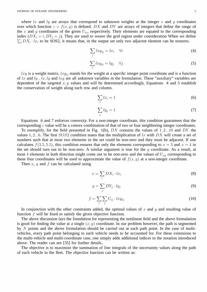
where lx and ly are arrays that correspond to unknown weights at the integerx and y coordinatesover which functionz = f(x, y) is defined.DX andDY are arrays of integers that define the range ofthe x and y coordinates of the givenUij, respectively. Their elements are equated to the correspondingindex (DXi = i, DYj = j). They are used to weave the grid region under considerationWhen we define∑

i DXi · lxi to be SOS2, it means that, in the output set only two adjacent element can be nonzero.

∑

j

lxyij = lxi ∀i (4)

∑

i

lxyij = lyj ∀j (5)

lxy is a weight matrix.lxyij stands for the weight at a specific integer point coordinate and is a functionof lx and ly . lx, ly and lxy are all unknown variables in the formulation. These ”auxiliary” variables aredependent of the targetedx, y values and will be determined accordingly. Equations 4 and 5establishthe conservation of weight along each row and column.

∑

i

lxi = 1 (6)

∑

j

lyj = 1 (7)

Equations 6 and 7 enforces convexity. For a non-integer coordinate, this condition guarantees that thecorrespondingz value will be a convex combination of that of two or four neighboring integer coordinates.

To exemplify, for the field presented in Fig 1(b),DX contains the values of1, 2...10 and DY thevalues1, 2...6. The firstSOS2 condition states that the multiplication oflx with DX will create a set ofnumbers such that at most two elements in the set could be non-zero and they must be adjacent. If onecalculatesf(3.5, 5.5), this condition ensures that only the elements corresponding to x = 3 andx = 4 inthe set should turn out to be non-zero. A similar argument is true for they coordinate. As a result, atmost4 elements in both direction might come out to be non-zero and the values ofUxy corresponding tothese four coordinates will be used to approximate the valueof f(x, y) at a non-integer coordinate.

Thenx, y andf can be calculated using

x =∑

i

DXi · lxi (8)

y =∑

j

DYj · lyj (9)

f =∑

i

∑

j

Uij · lxyij (10)

In conjunction with the other constraints added, the optimal values ofx and y and resulting value offunction f will be fixed to satisfy the given objective function.

The above discussion lays the foundation for representing the nonlinear field and the above formulationis good for finding the value at a single(x, y) coordinate. In our problem however, the path is segmentedby N points and the above formulation should be carried out at each path point. In the case of multi-vehicles, every path point belonging to each vehicle needs to be accounted for. For these extensions tothe multi-vehicle and multi-coordinate case, one simply adds additional indices to the notation introducedabove. The reader can see [35] for further details.

The objective is to maximize the summation of line integralsof the uncertainty values along the pathof each vehicle in the fleet. The objective function can be written as:


maxP∑

p=1

Np∑

k=1

fpk (11)

whereP is the total number of vehicles in the fleet andNp is the total number of path-points belongingto thepth vehicle. In all of the above equations, subscriptsp andk stand to denote thekth path-point ofpth

vehicle.Uij (which is composed of the discretized values of the functionz = f(x, y) on the computational2D grid) stands for the uncertainty field data which is the input to our problem.

IV. M OTION CONSTRAINTS

For the vehicles to move in a desired manner, some constraints that shape the vehicle navigation areneeded: primary motion, anti-curling, vicinity, communications and obstacle avoidance constraints.

A. Primary Motion Constraints

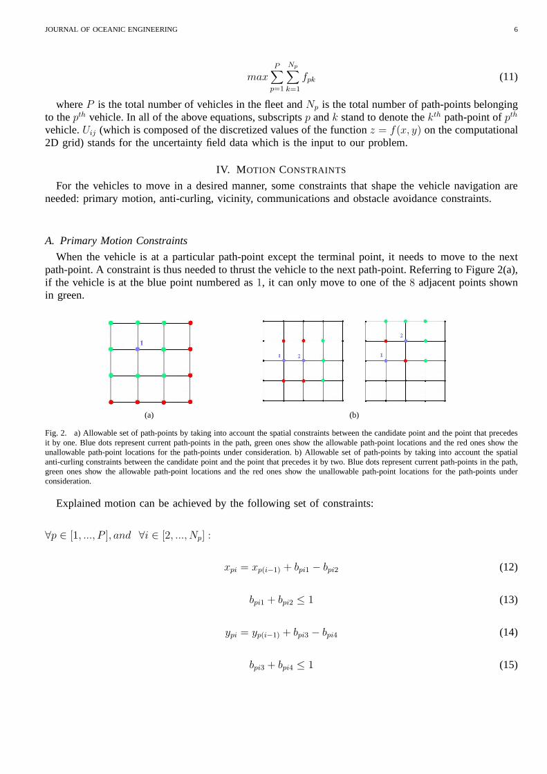
When the vehicle is at a particular path-point except the terminal point, it needs to move to the nextpath-point. A constraint is thus needed to thrust the vehicle to the next path-point. Referring to Figure 2(a),if the vehicle is at the blue point numbered as1, it can only move to one of the8 adjacent points shownin green.

(a) (b)

Fig. 2. a) Allowable set of path-points by taking into account the spatial constraints between the candidate point and the point that precedesit by one. Blue dots represent current path-points in the path, green ones show the allowable path-point locations and the red ones show theunallowable path-point locations for the path-points under consideration. b) Allowable set of path-points by taking into account the spatialanti-curling constraints between the candidate point and the point that precedes it by two. Blue dots represent currentpath-points in the path,green ones show the allowable path-point locations and the red ones show the unallowable path-point locations for the path-points underconsideration.

Explained motion can be achieved by the following set of constraints:

∀p ∈ [1, ..., P ], and ∀i ∈ [2, ..., Np] :

xpi = xp(i−1) + bpi1 − bpi2 (12)

bpi1 + bpi2 ≤ 1 (13)

ypi = yp(i−1) + bpi3 − bpi4 (14)

bpi3 + bpi4 ≤ 1 (15)


∀p ∈ [1, ..., P ], and ∀i ∈ [2, ..., Np] :

bpi1 + bpi2 + bpi3 + bpi4 ≥ 1 (16)

∀p ∈ [1, ..., P ], ∀i ∈ [2, ..., Np], and ∀j ∈ [1, ..., 4] :

bpij ∈ 0, 1 (17)

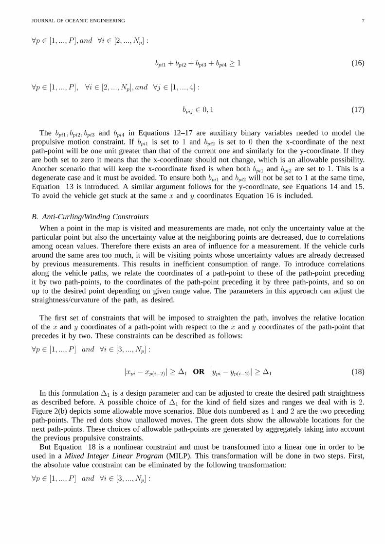
The bpi1, bpi2, bpi3 and bpi4 in Equations 12–17 are auxiliary binary variables needed tomodel thepropulsive motion constraint. Ifbpi1 is set to1 and bpi2 is set to0 then the x-coordinate of the nextpath-point will be one unit greater than that of the current one and similarly for the y-coordinate. If theyare both set to zero it means that the x-coordinate should notchange, which is an allowable possibility.Another scenario that will keep the x-coordinate fixed is when both bpi1 and bpi2 are set to1. This is adegenerate case and it must be avoided. To ensure bothbpi1 andbpi2 will not be set to1 at the same time,Equation 13 is introduced. A similar argument follows for the y-coordinate, see Equations 14 and 15.To avoid the vehicle get stuck at the samex andy coordinates Equation 16 is included.

B. Anti-Curling/Winding Constraints

When a point in the map is visited and measurements are made, not only the uncertainty value at theparticular point but also the uncertainty value at the neighboring points are decreased, due to correlationsamong ocean values. Therefore there exists an area of influence for a measurement. If the vehicle curlsaround the same area too much, it will be visiting points whose uncertainty values are already decreasedby previous measurements. This results in inefficient consumption of range. To introduce correlationsalong the vehicle paths, we relate the coordinates of a path-point to these of the path-point precedingit by two path-points, to the coordinates of the path-point preceding it by three path-points, and so onup to the desired point depending on given range value. The parameters in this approach can adjust thestraightness/curvature of the path, as desired.

The first set of constraints that will be imposed to straighten the path, involves the relative locationof the x andy coordinates of a path-point with respect to thex andy coordinates of the path-point thatprecedes it by two. These constraints can be described as follows:

∀p ∈ [1, ..., P ] and ∀i ∈ [3, ..., Np] :

|xpi − xp(i−2)| ≥ ∆1 OR |ypi − yp(i−2)| ≥ ∆1 (18)

In this formulation∆1 is a design parameter and can be adjusted to create the desired path straightnessas described before. A possible choice of∆1 for the kind of field sizes and ranges we deal with is2.Figure 2(b) depicts some allowable move scenarios. Blue dots numbered as1 and2 are the two precedingpath-points. The red dots show unallowed moves. The green dots show the allowable locations for thenext path-points. These choices of allowable path-points are generated by aggregately taking into accountthe previous propulsive constraints.

But Equation 18 is a nonlinear constraint and must be transformed into a linear one in order to beused in aMixed Integer Linear Program(MILP). This transformation will be done in two steps. First,the absolute value constraint can be eliminated by the following transformation:

∀p ∈ [1, ..., P ] and ∀i ∈ [3, ..., Np] :


xpi − xp(i−2) ≥ ∆1

or xp(i−2) − xpi ≥ ∆1

or ypi − yp(i−2) ≥ ∆1

or yp(i−2) − ypi ≥ ∆1 (19)

Equation 19 is a disjunctive constraint and is not a suitablekind of constraint for a MILP formulation.Constraints in a MILP formulation must be conjunctive. It ispossible to transform a disjunctive constraintinto a conjunctive one by using auxiliary binary variables and “Big-M” constants [36]. Such transformationyields:

∀p ∈ [1, ..., P ] and ∀i ∈ [3, ..., Np] :

xpi − xp(i−2) ≥ ∆1 − M ∗ t1pi1

and xp(i−2) − xpi ≥ ∆1 − M ∗ t1pi2

and ypi − yp(i−2) ≥ ∆1 − M ∗ t1pi3

and yp(i−2) − ypi ≥ ∆1 − M ∗ t1pi4 (20)

and4∑

w=1

t1piw ≤ 3 (21)

t1piw ∈ 0, 1 ∀w ∈ [1, ..., 4] (22)

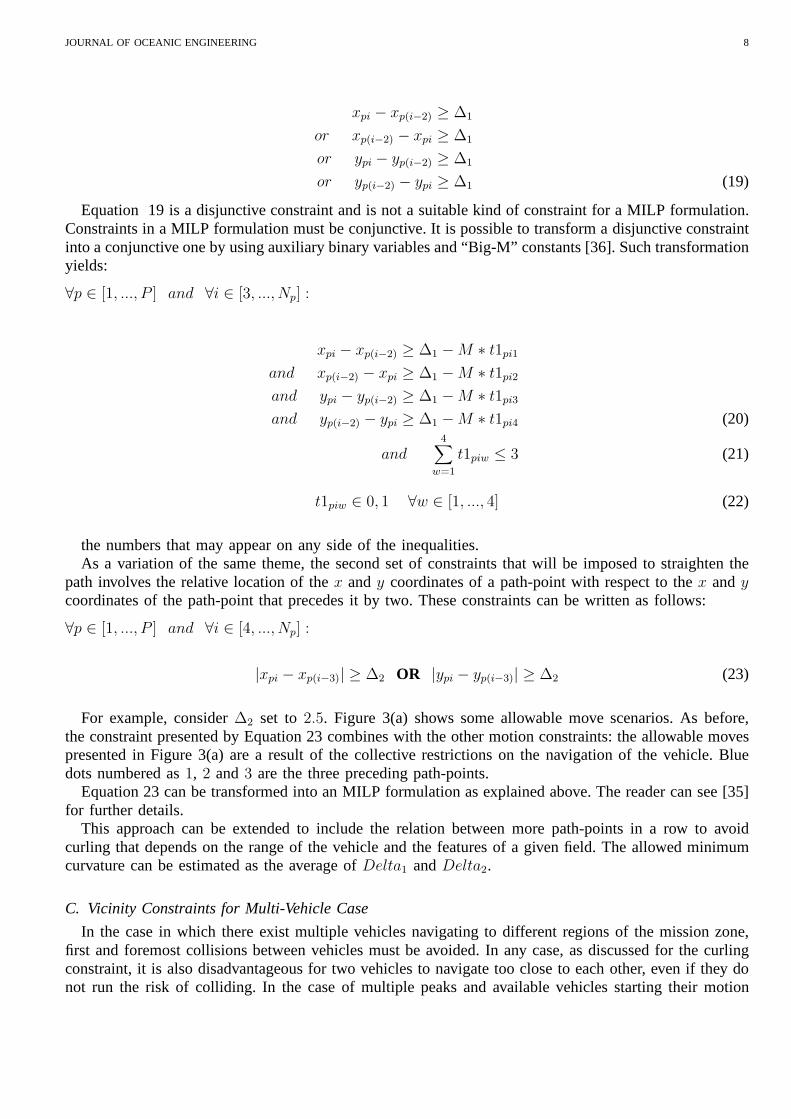
the numbers that may appear on any side of the inequalities.As a variation of the same theme, the second set of constraints that will be imposed to straighten the

path involves the relative location of thex andy coordinates of a path-point with respect to thex andy

coordinates of the path-point that precedes it by two. Theseconstraints can be written as follows:

∀p ∈ [1, ..., P ] and ∀i ∈ [4, ..., Np] :

|xpi − xp(i−3)| ≥ ∆2 OR |ypi − yp(i−3)| ≥ ∆2 (23)

For example, consider∆2 set to2.5. Figure 3(a) shows some allowable move scenarios. As before,the constraint presented by Equation 23 combines with the other motion constraints: the allowable movespresented in Figure 3(a) are a result of the collective restrictions on the navigation of the vehicle. Bluedots numbered as1, 2 and3 are the three preceding path-points.

Equation 23 can be transformed into an MILP formulation as explained above. The reader can see [35]for further details.

This approach can be extended to include the relation between more path-points in a row to avoidcurling that depends on the range of the vehicle and the features of a given field. The allowed minimumcurvature can be estimated as the average ofDelta1 andDelta2.

C. Vicinity Constraints for Multi-Vehicle Case

In the case in which there exist multiple vehicles navigating to different regions of the mission zone,first and foremost collisions between vehicles must be avoided. In any case, as discussed for the curlingconstraint, it is also disadvantageous for two vehicles to navigate too close to each other, even if they donot run the risk of colliding. In the case of multiple peaks and available vehicles starting their motion


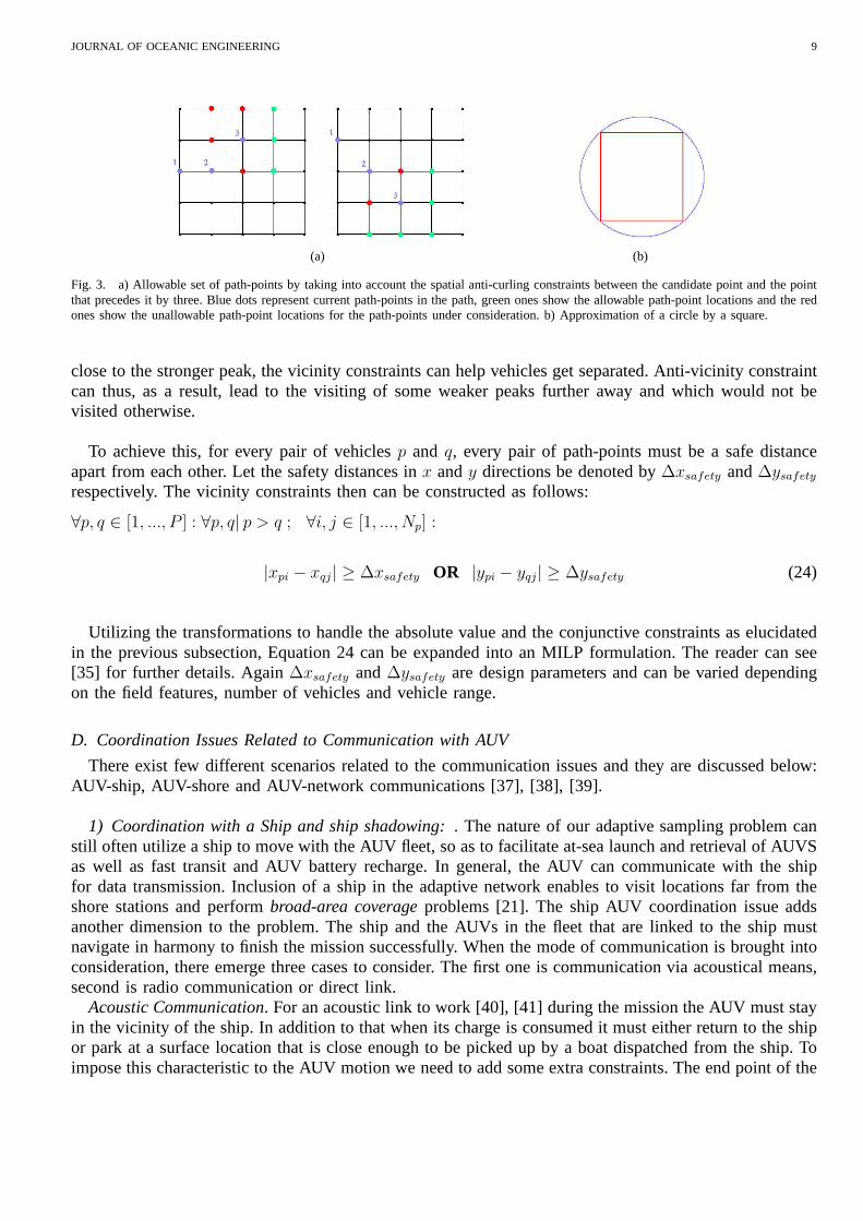
(a) (b)

Fig. 3. a) Allowable set of path-points by taking into account the spatial anti-curling constraints between the candidate point and the pointthat precedes it by three. Blue dots represent current path-points in the path, green ones show the allowable path-pointlocations and the redones show the unallowable path-point locations for the path-points under consideration. b) Approximation of a circle by a square.

close to the stronger peak, the vicinity constraints can help vehicles get separated. Anti-vicinity constraintcan thus, as a result, lead to the visiting of some weaker peaks further away and which would not bevisited otherwise.

To achieve this, for every pair of vehiclesp and q, every pair of path-points must be a safe distanceapart from each other. Let the safety distances inx andy directions be denoted by∆xsafety and∆ysafety

respectively. The vicinity constraints then can be constructed as follows:

∀p, q ∈ [1, ..., P ] : ∀p, q| p > q ; ∀i, j ∈ [1, ..., Np] :

|xpi − xqj | ≥ ∆xsafety OR |ypi − yqj| ≥ ∆ysafety (24)

Utilizing the transformations to handle the absolute valueand the conjunctive constraints as elucidatedin the previous subsection, Equation 24 can be expanded intoan MILP formulation. The reader can see[35] for further details. Again∆xsafety and∆ysafety are design parameters and can be varied dependingon the field features, number of vehicles and vehicle range.

D. Coordination Issues Related to Communication with AUV

There exist few different scenarios related to the communication issues and they are discussed below:AUV-ship, AUV-shore and AUV-network communications [37],[38], [39].

1) Coordination with a Ship and ship shadowing:. The nature of our adaptive sampling problem canstill often utilize a ship to move with the AUV fleet, so as to facilitate at-sea launch and retrieval of AUVSas well as fast transit and AUV battery recharge. In general,the AUV can communicate with the shipfor data transmission. Inclusion of a ship in the adaptive network enables to visit locations far from theshore stations and performbroad-area coverageproblems [21]. The ship AUV coordination issue addsanother dimension to the problem. The ship and the AUVs in thefleet that are linked to the ship mustnavigate in harmony to finish the mission successfully. Whenthe mode of communication is brought intoconsideration, there emerge three cases to consider. The first one is communication via acoustical means,second is radio communication or direct link.

Acoustic Communication. For an acoustic link to work [40], [41] during the mission the AUV must stayin the vicinity of the ship. In addition to that when its charge is consumed it must either return to the shipor park at a surface location that is close enough to be pickedup by a boat dispatched from the ship. Toimpose this characteristic to the AUV motion we need to add some extra constraints. The end point of the


AUV can either be specified to be the coordinate of the ship, orstay in the same vicinity of the vehicleas the rest of the path-points, or it can be dictated that although it does not need to be same as the shipcoordinates (meaning return to the ship) it should be closerto the ship than the rest of the path-points.Also in order to synchronize the motion of the ship and the AUVfleet the path of the ship must beknown. Once the ship path is known (ship path can be determined using ideas and methods similar to theones presented in this paper) it can be segmented into as manypath-points as the AUV. Then, the timedomain dependence is unique between identically indexed ship and AUV path points. Thenth path-pointof the ship then corresponds to the location of the ship when the AUV visits its nth path-point. If allAUVs in the fleet have same number of path-points, a single segmentation is enough, if they do not thenthe ship path segmentation must be performed for every AUV. Assuming that the terminal path-point ofthe AUV stays within the same distance to the ship as the otherpath-points, these ideas can be put intoMILP formulation as follows:

∀p ∈ [1, ..., P ] ∀i ∈ [1, ..., Np] :

|xpi − ship xpi| ≤ ∆xship vicinity AND (25)

|ypi − ship ypi| ≤ ∆yship vicinity

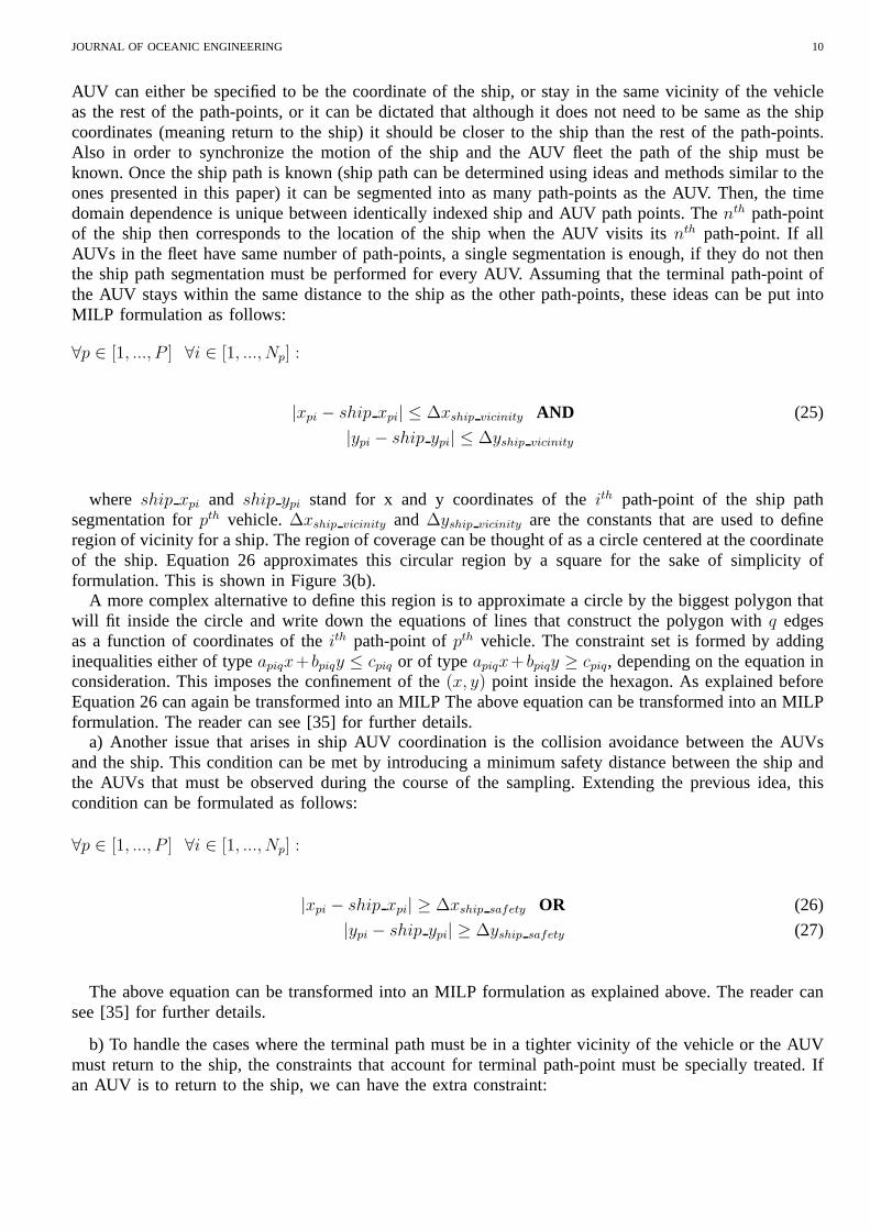
where ship xpi and ship ypi stand for x and y coordinates of theith path-point of the ship pathsegmentation forpth vehicle.∆xship vicinity and ∆yship vicinity are the constants that are used to defineregion of vicinity for a ship. The region of coverage can be thought of as a circle centered at the coordinateof the ship. Equation 26 approximates this circular region by a square for the sake of simplicity offormulation. This is shown in Figure 3(b).

A more complex alternative to define this region is to approximate a circle by the biggest polygon thatwill fit inside the circle and write down the equations of lines that construct the polygon withq edgesas a function of coordinates of theith path-point ofpth vehicle. The constraint set is formed by addinginequalities either of typeapiqx+ bpiqy ≤ cpiq or of typeapiqx+ bpiqy ≥ cpiq, depending on the equation inconsideration. This imposes the confinement of the(x, y) point inside the hexagon. As explained beforeEquation 26 can again be transformed into an MILP The above equation can be transformed into an MILPformulation. The reader can see [35] for further details.

a) Another issue that arises in ship AUV coordination is the collision avoidance between the AUVsand the ship. This condition can be met by introducing a minimum safety distance between the ship andthe AUVs that must be observed during the course of the sampling. Extending the previous idea, thiscondition can be formulated as follows:

∀p ∈ [1, ..., P ] ∀i ∈ [1, ..., Np] :

|xpi − ship xpi| ≥ ∆xship safety OR (26)

|ypi − ship ypi| ≥ ∆yship safety (27)

The above equation can be transformed into an MILP formulation as explained above. The reader cansee [35] for further details.

b) To handle the cases where the terminal path must be in a tighter vicinity of the vehicle or the AUVmust return to the ship, the constraints that account for terminal path-point must be specially treated. Ifan AUV is to return to the ship, we can have the extra constraint:


xpNp= ship xpNp

∀p ∈ [1, ..., P ]

ypNp= ship ypNp

∀p ∈ [1, ..., P ] (28)

c) Or if the terminal path-point needs to lie in a tighter vicinity than the other path-points for the easeof picking up, then we need to add the constraints:

∀p ∈ [1, ..., P ] :

|xpNp− ship xpNp

≤ ∆xship vicinity TP OR

|ypNp− ship ypNp

≤ ∆yship vicinity TP (29)

where∆xship vicinity TP and∆yship vicinity TP stand for the tighter bounds on the vicinity of terminalpath-points to the ship. The above equation can be transformed into an MILP formulation as explainedabove. The reader can see [35] for further details.

Radio and direct communications. As aforementioned, the two other alternatives for communicationare the radio link and the direct communication. If the preferred way of communication is opted to bewireless communication (radio) the AUV needs to be in some vicinity of the ship at the end of its motionto communnicate with the ship. In that case only the Equation29 needs to apply.

If direct connection is the selected communication method,the AUV needs to board the ship at the endof the mission and in which case, only Equation 28 needs to be applied.

2) Communication with a Shore Station:In the case of shore station, the end path-point coordinatesof the vehicles need to either lie in a vicinity of the stationlocation to establish radio communicationor they must match with the coordinates of the shore station if they are required to return to it. If thevehicles need to lie in a proximity of the shore station to be picked up by a boat, we need to introducethe constraints:

∀p ∈ [1, ..., P ] :

xpNp− shore x ≤ ∆xshore vicinity + M ∗ s3xp1

and shore x − xpNp≤ ∆xshore vicinity + M ∗ s3xp2

and ypNp− shore y ≤ ∆yshore vicinity + M ∗ s3yp1

and shore y − ypNp≤ ∆yshore vicinity + M ∗ s3yp2 (30)

and2∑

w=1

s3xpw ≤ 1 (31)

and2∑

w=1

s3ypw ≤ 1 (32)

s3xpw, s3ypw ∈ 0, 1 ∀w ∈ [1, ..., 2] (33)


where,shore x and shore y stand for the x and y coordinates of the shore station. Or, if the vehicleneeds to return to the shore station, one can impose:

xpNp= shore x ∀p ∈ [1, ..., P ]

ypNp= shore y ∀p ∈ [1, ..., P ] (34)

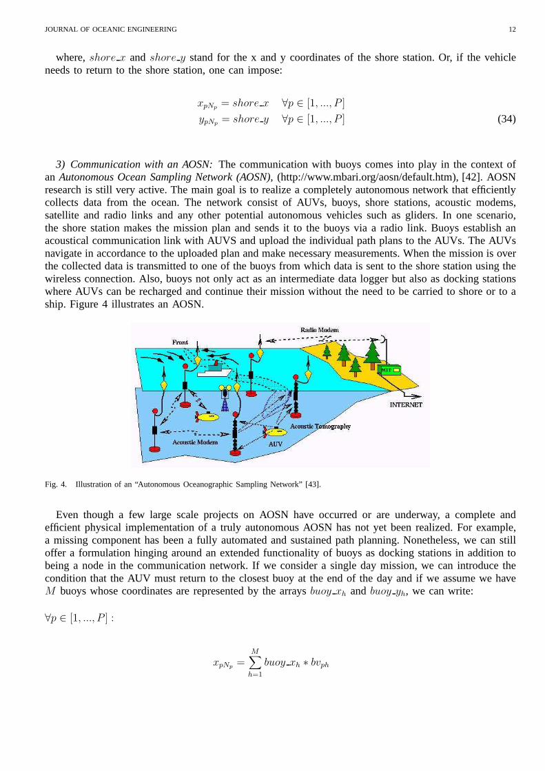
3) Communication with an AOSN:The communication with buoys comes into play in the context ofan Autonomous Ocean Sampling Network (AOSN), (http://www.mbari.org/aosn/default.htm), [42]. AOSNresearch is still very active. The main goal is to realize a completely autonomous network that efficientlycollects data from the ocean. The network consist of AUVs, buoys, shore stations, acoustic modems,satellite and radio links and any other potential autonomous vehicles such as gliders. In one scenario,the shore station makes the mission plan and sends it to the buoys via a radio link. Buoys establish anacoustical communication link with AUVS and upload the individual path plans to the AUVs. The AUVsnavigate in accordance to the uploaded plan and make necessary measurements. When the mission is overthe collected data is transmitted to one of the buoys from which data is sent to the shore station using thewireless connection. Also, buoys not only act as an intermediate data logger but also as docking stationswhere AUVs can be recharged and continue their mission without the need to be carried to shore or to aship. Figure 4 illustrates an AOSN.

Fig. 4. Illustration of an “Autonomous Oceanographic Sampling Network” [43].

Even though a few large scale projects on AOSN have occurred or are underway, a complete andefficient physical implementation of a truly autonomous AOSN has not yet been realized. For example,a missing component has been a fully automated and sustainedpath planning. Nonetheless, we can stilloffer a formulation hinging around an extended functionality of buoys as docking stations in addition tobeing a node in the communication network. If we consider a single day mission, we can introduce thecondition that the AUV must return to the closest buoy at the end of the day and if we assume we haveM buoys whose coordinates are represented by the arraysbuoy xh and buoy yh, we can write:

∀p ∈ [1, ..., P ] :

xpNp=

M∑

h=1

buoy xh ∗ bvph


ypNp=

M∑

h=1

buoy yh ∗ bvph

(35)

M∑

h=1

bvph = 1 ∀p ∈ [1, ..., P ] (36)

bvph ∈ 0, 1 ∀h ∈ [1, ..., M ] (37)

Variablesbvph are auxiliary variables that help to choose one of the buoy coordinates as the end pointcoordinate of AUVs. Equation 36 guarantees that only one buoy coordinate will be assigned to a specificAUV. Also depending on the docking capabilities of an buoy wecan impose the constraint that at mostone AUV can park at a given buoy. This can be formulated as:

N∑

p=1

bvph ≤ 1 ∀h ∈ [1, ..., M ] (38)

Other constraints related to the communication with buoys or some other constraint that cannot beforeseen at this time without an actual implementation of anAOSN might need to be added. Given theflexibility and strength of the suggested formulation framework, other requirements that could emergedepending on the specific implementation of an AOSN can easily be added to the formulation.

E. Obstacle Avoidance

In the case of existence of obstacles in the region of interest, the task of collision prevention withobstacles could be managed in two alternative ways. One option is to introduce inequalities which willremove the regions where obstacles lie from the feasible coordinate set of the vehicle navigation. Another,simpler approach is to set the uncertainty values within theregions occupied by the obstacles to a verylarge negative number. Those points will not be included in the solution since their inlusion will havenegative contribution to the objective function. For otherapproaches on obstacle avoidance, we refer to[44], [45], [46], [47].

V. M ETHODOLOGY AND SOFTWARE SELECTION FOR THEMILP SOLUTION

Our choice of implementation platform is XPress-MP optimization package from “Dash Optimization”(http://www.dashoptimization.com). It has a MILP solver which uses brand and bound algorithm. It issuitable for solving our path planning problem.

For optimum performance and ease of development, the ideal is to use a high level modeling lan-guage that is compatible with the solver. Such modeling languages are especially made for optimizationproblems and are equipped with powerful tools to implement optimization problems faster. A modelinglanguage offered by Dash Optimization isMosel. Implementing the mathematical program inMosel isstraightforward, requiring minimal translation from the canonical form shown in Equations 2–38. Also,Mosel is capable of easily implementing theSOS2.constraints.


VI. RESULTS FORSINGLE-DAY CASE

Our methodology and software have been tried on a wide variety of different scenarios with multipletypes of fleet sizes, ranges, starting points and constraints. The ocean fields that have been used are thetemperature forecast uncertainty maps in Monterey Bay during August-September 2003, as calculated bythe Harvard Ocean Prediction System (HOPS) and Error Subspace Statistical Estimation (ESSE) system(see Sect 2). In the examples that follow, most examples shown are for August27, 2003 and utilizeuncertainty averages from the upper [0−40]m ocean layers, focusing on largest uncertainties in the oceansurface mixed-layer and ocean thermocline dynamics. Depending on the objective, velocity or salinityfields (or even a weighted average of all fields) can also be used with our software.

In all of the following graphs grey dots indicate the starting point of the motion, white dots indicatethe final point on the path. One important parameter in the problem formulation that controls the rangefor a given vehicle is the number of path-points, “Np”. It is not directly equal to the range since diagonalmoves are allowed. Its value must be chosen based on the allowable range for each AUV on a given day.Once the problem is solved with the initial selection for “Np”, depending on the length of the generatedpath, some iterations might be necessary.

A. Results for Single-Vehicle Case

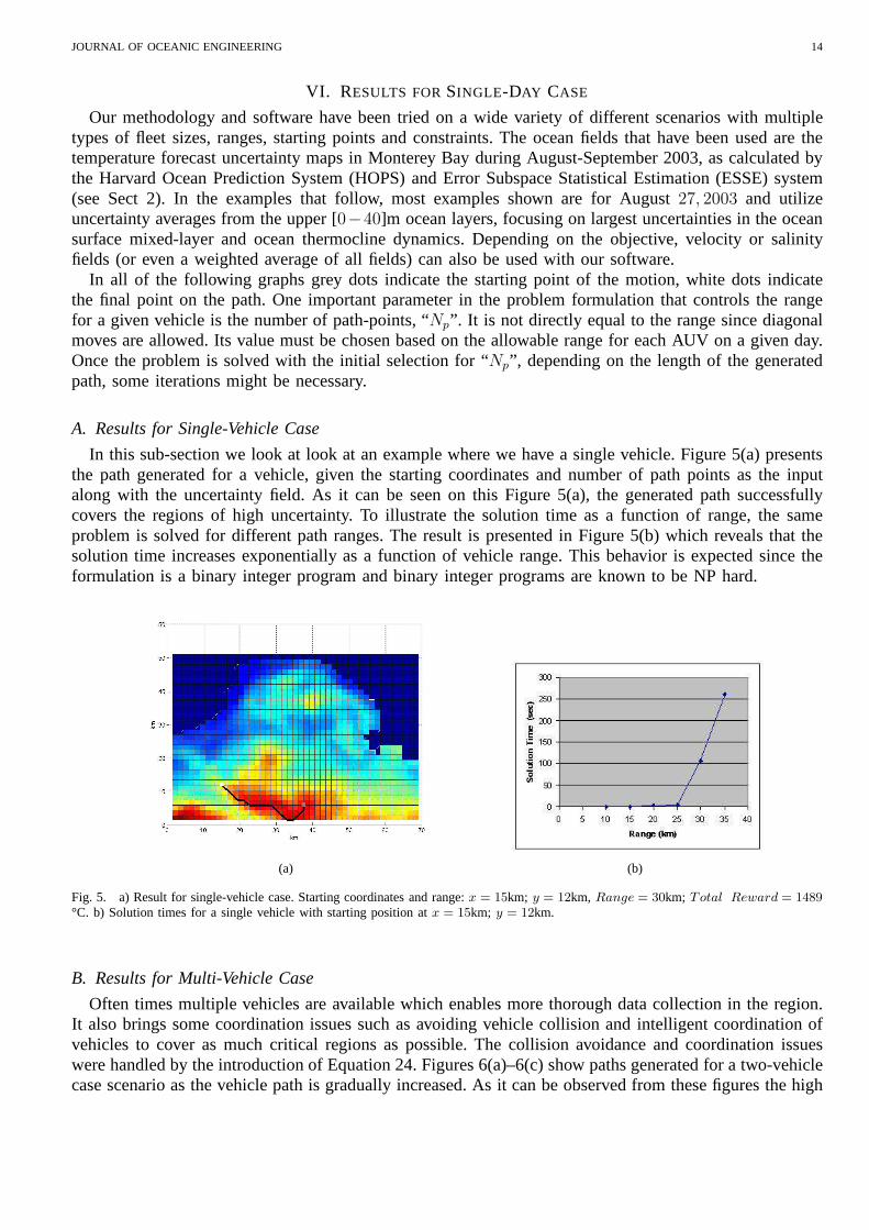
In this sub-section we look at look at an example where we havea single vehicle. Figure 5(a) presentsthe path generated for a vehicle, given the starting coordinates and number of path points as the inputalong with the uncertainty field. As it can be seen on this Figure 5(a), the generated path successfullycovers the regions of high uncertainty. To illustrate the solution time as a function of range, the sameproblem is solved for different path ranges. The result is presented in Figure 5(b) which reveals that thesolution time increases exponentially as a function of vehicle range. This behavior is expected since theformulation is a binary integer program and binary integer programs are known to be NP hard.

(a) (b)

Fig. 5. a) Result for single-vehicle case. Starting coordinates and range:x = 15km; y = 12km, Range = 30km; Total Reward = 1489

°C. b) Solution times for a single vehicle with starting position at x = 15km; y = 12km.

B. Results for Multi-Vehicle Case

Often times multiple vehicles are available which enables more thorough data collection in the region.It also brings some coordination issues such as avoiding vehicle collision and intelligent coordination ofvehicles to cover as much critical regions as possible. The collision avoidance and coordination issueswere handled by the introduction of Equation 24. Figures 6(a)–6(c) show paths generated for a two-vehiclecase scenario as the vehicle path is gradually increased. Asit can be observed from these figures the high


uncertainty regions are efficiently covered. The solution times are presented in Figure 6(d) which againincreases exponentially as a function of path-points.

(a) (b)

(c) (d)

Fig. 6. a) Result for two-vehicle case. Starting coordinates and ranges:x1 = 15km, y1 = 22.5km, Range1 = 15km; x2 = 45km,y2 = 15km, Range2 = 14km; Total Reward = 972°C. b) Result for two-vehicle case. Starting coordinates and ranges:x1 = 15km,y1 = 22.5km, Range1 = 16.5km; x2 = 45km, y2 = 15km, Range2 = 18km; Total Reward = 1273 °C. c) Result for two-vehiclecase. Starting coordinates and ranges:x1 = 15km, y1 = 22.5km, Range1 = 22.5km; x2 = 45km; y2 = 15km, Range2 = 24km;Total Reward = 1879 °C. d) Solution times for two vehicles with starting positions x1 = 15km, y1 = 22.5km ; x2 = 45km; y2 = 15km.

C. Vehicle Number Sensitivity

The aim of this section is to show the sensitivity of the solution time to the number of vehicles involvedin the path planning task. We start with one vehicle and at each step introduce another vehicle until wereach five vehicles. Of course, each time a vehicle is added, anew global MILP optimization is carriedout for all vehicles present. The path of all vehicles are optimized at once. The results are presentedin Figures 7(a)–7(e). The solution times are presented in Figure ??(f). There is a sudden increase asthe number of vehicles increase. This behavior is in agreement with the exponential complexity of theproblem. Note that in this illustration of the sensitivity to the number of vehicles, the starting points ofvehicles are selected far apart from each other deliberately so that the addition of another vehicle doesnot affect the previous solution by much. This peculiar behavior allows more direct comparisons withprevious illustrations.


D. Results with Ship Shadowing

As explained earlier, during a mission, AUVs are generally accompanied by a ship. The AUVs aredropped from the ship for their mission and dock to, or are collected by, the ship at the end. To handlethis situation, extra constraints are added to the formulation. The constraints to be used depend on thetype of communication (see Sect 4.D).

Figures 8(a)-(b) show two cases where the preferred mode of communication is chosen to be acoustical.Equations 26 and IV-D.1 are utilized in our formulation. Thefirst case, where the defined proximity isset to be15km takes9sec to solve. When the proximity value is decreased to9 the solution time alsodecreases to5.25sec. The improvement is expected since tightening the constraint also shrinks the searchspace, resulting to strides in the solution time.

Another possible scenario is when the communication is via direct link in which case the AUVs do notneed to stay in the vicinity of the ship throughout their mission, but must either park in some proximityof the ship or return to the ship at the end of their travel. This time Equations 28–29 are used. Figure 8(c)and Figure 8(d) present examples of the latter and former cases respectively. The region of proximity isdefined to be3km for Figure 8(c). The solution time is2.3sec. For the case where AUVs need to returnto the ship the solution time is2.14sec.

VII. T IME PROGRESSIVEPATH PLANNING

Up until this point, the sampling task had been assumed to take place in a single day without anypertinence to previous or following days. This is a perfectly fine scenario in rapid assessment in oceanog-raphy and it has been very successful for multiple uses at sea[6], [18]–[20], [48], [49]. However, a moresophisticated situation emerges when the sampling task hasto be carried out over multiple days. In suchtime-evolving situations, the regions of high uncertaintyare moving and transforming in shape as timeprogresses [4], [50] and the adaptive sampling fleet must adapt to the dynamic uncertainty field. In suchscenarios, it is necessary to have some information exchange and coordination between the paths of thevehicles that are expected to be realized on consecutive days, so as to satisfy path optimality over bothspace and time.

Implementation a time dimension is introduced both for the primary and auxiliary variables. Everyvariable must have a new index that represents which day theybelong to. The new objective function isthen a summation of rewards from all days in consideration. Akey point in establishing the link betweenconsecutive days and introducing time-progressive features is to define the relation between the end path-point of vehicles on one day with the starting point on the following day. One option is to introduce theconstraint that the starting point of the vehicle for a consecutive mission day should lie within a vicinity ofthe end point of the previous day. Another option is to imposethe constraint that on consecutive missiondays the vehicles should start their mission exactly at the end location of the previous day. This latterconstraint can be defined as:

∀p ∈ [1, ..., P ], ∀d ∈ [2, ..., D] :

xpd1 = xp(d−1)Np(39)

ypd1 = yp(d−1)Np(40)

where D stands for the total number of mission days. To further exemplify the inclusion of timedimension, the objective function can be written as:

Maximize

P∑

p=1

D∑

d=1

Np∑

k=1

fpdk (41)


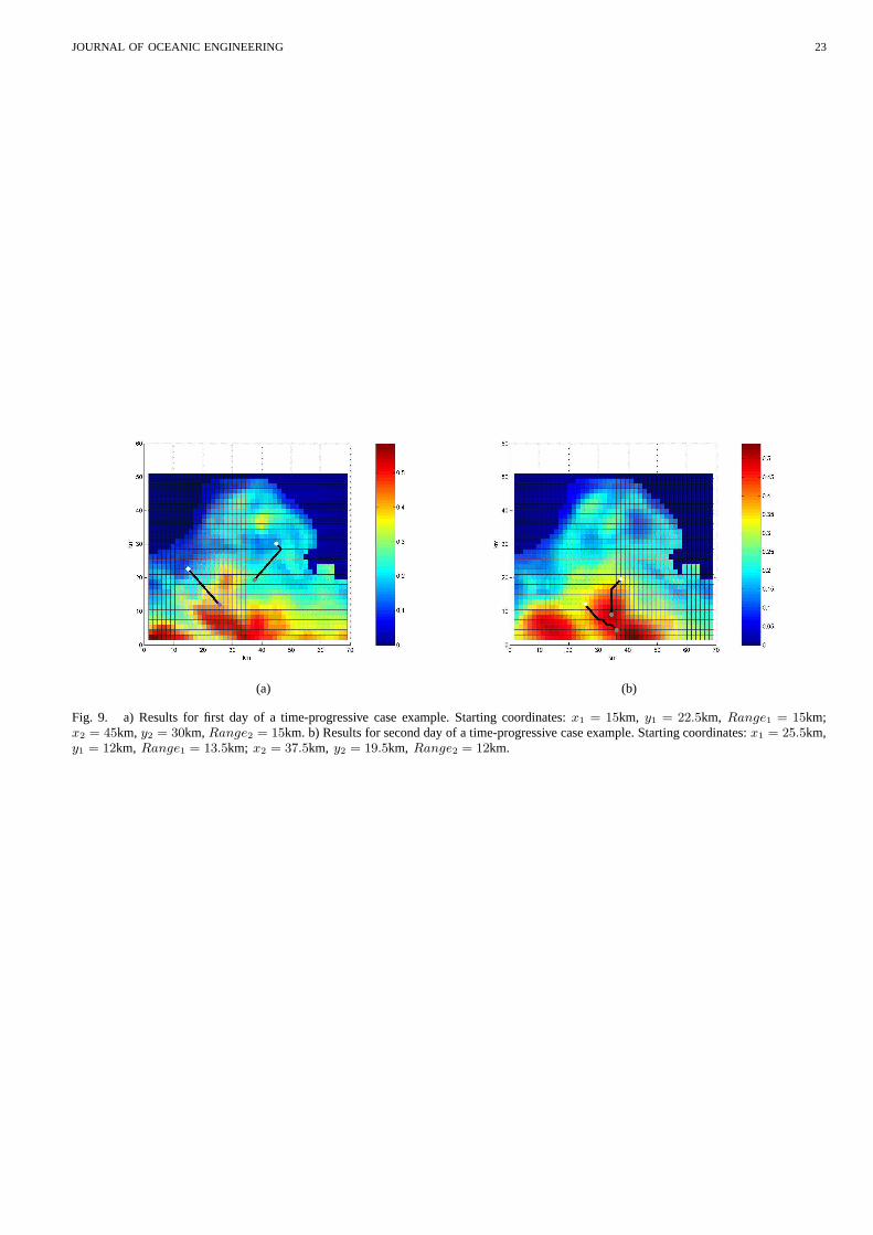
The reader can see [35] for the full formulation for time progressive case. Assuming that AUVs haveenough total range to complete sampling over the defined duration without any need to dock to getrecharged and they continue their mission at the end point ofthe previous day, an example problem issolved whose results are presented in Figure 9. This examplealso reveals capabilities of the proposedformulation to find time global optimal solutions. The number of path-points chosen for both vehicles onboth days is8, which leads to a range of15km per day. If we assume the absence of any information linkbetween the uncertainty data for day1 and day2, looking at Figure 9(a), on day1 the second vehicle,which starts its motion at x=45km and y=30km, would have needed to be close to the small peak locatedaround x=40km, y=35km. With the 2-day information available, vehicle2 moves on day1 such as shownon Figure 9(a). Since there is a constrained connection between day1 and day2, vehicle2 compromiseson the total amount of reward it can collect on day1 ,and heads towards the high-uncertainty region thatis predicted to form on day2 around x=35km, y=10km. Over the two days, this enables the maximizationof total reward, in the present case, the visit of high uncertainty regions.

The above discussion can be easily extended to3−D case by simply adding an index for z coordinateto most of the variables involved in the formulation. This adds some new formulation variables related tothe additional z coordinate and modifies the right-hand-sides of some of the inequalities.

VIII. C ONCLUSIONS AND DISCUSSIONS

In this paper we have addressed the problem of path planning of Autonomous Underwater Vehicles(AUVs) for adaptive sampling. We introduced an MILP based formulation which is capable of handlingmulti-vehicle and multi-day cases. Using MILP formulationtechniques it is possible to successfully modelall the constraints needed for different problem scenarios. The strength of the MILP formulation makesfuture problem formulation extensions and modifications possible. This point was exemplified within theAutonomous Ocean Sampling Network (AOSN)concept, (http://www.mbari.org/aosn/default.htm), [42].

We first developed the details of our optimization formulation, including the objective function and awide range of constraints. Once formulated, we implementedand solved the problem using the XPress-MP optimization suit from “Dash optimization”. We preferred to use the native optimization formulationenvironment from Dash Optimization called Mosel to manage the formulation task. However, the formu-lation can be easily implemented with other optimization solver platforms. Using our new approach, wedemonstrated a set of results for a wide range of scenarios using realistic ocean uncertainty fields. Theeffects of variations on the type of constraints, number of vehicles and time-dependence were studiedand diverse sensitivity studies carried out. In all cases, the results show that the method is capable ofgenerating desired solutions within allotted time limits.

The problem we study is an NP hard problem. Therefore, as the problem size increases the solution timeincreases exponentially. For the sizes we considered the solution time was short, especially in comparisonto the time required to compute forecast ocean fields and their uncertainties. Our path planning resultswere obtained on Pentium4, 2.8 GHz computer with1 GByte of RAM. For larger problems, fastermachines and grid/parallel computing are two options. The XPress-MP optimization suit we used alreadysupport parallel computing. i

There remain many directions for future research. For example, the correlation between the measurementperformed at one location and the change of uncertainty values around that location as a result of thecollected data, can been taken into direct consideration. In future work, we are planning to establish thelink between a measurement performed at a generated path-point and its effect on uncertainty field orfields involved in the problem, including the Error SubspaceStatistical Estimation (ESSE) technique intoour optimization framework. Another line of research is theutilization of XML schemes [51] that controlthe parameters of our path planning schemes and couple the optimization with the ocean modeling anddata assimilation schemes.

The framework we supplied can also be extended to be utilizedat low-level path planning wherelinearized vehicle dynamics and some way-point information coming from high-level programming can


be combined to smoothen the path in an optimal manner. Another avenue of further research is the use ofalternative solution techniques that can quickly generatesuboptimal integer solutions and can warm-startthe branch and bound algorithms. Candidate techniques include genetic algorithms and development ofheuristics.

ACKNOWLEDGMENT

We thank the whole AOSN-II team and colleagues for their real-time work in Monterey Bay. Specialthanks go P. J. Haley, W. G. Leslie, A. R. Robinson, N. Leonard, H. Schmidt and D. Paley for collaborationson ocean modeling and adaptive sampling. We also like to thank to Prof. D. Pucci De Farias and Prof. J.Leonard for the valuable discussions. This work was funded in part by the National Science Foundation(under ITR grant EIA-0121263) and the Department of Commerce (under NOAA - MIT Sea Grant CollegeProgram grant NA86RG0074). P. F. J. Lermusiaux was supported by the Office of Naval Research undergrant N00014-05-1-0335, N00014-04-1-0534, N00014-05-G-0106 and N00014-05-1-0370.

REFERENCES

[1] M. Ehrendorfer, “Predicting the uncertainty of numerical weather forecasts: a review,”Meteorologische Zeitschrift, vol. 4, pp. 47–183,1997.

[2] P. F. J. Lermusiaux, “Data assimilation via error subspace statistical estimation, part ii: Middle atlantic bight shelfbreak front simulationsand esse validation,”Monthly Weather Review, vol. 127, no. 7, pp. 1408–1432, 1999.

[3] C. H. Bishop and Z. Toth, “Ensemble transformation and adaptive observations,”Journal of Atmospheric Sciences, vol. 56, pp. 1748–1765, 1999.

[4] P. F. J. Lermusiaux, C. S. Chiu, G. G. Gawarkiewicz, P. Abbot, A. R. Robinson, R. N. Miller, P. J. Haley, W. G. Leslie, S. J. Majumdar,A. Pang, and F. Lekien, “Quantifying uncertainities in ocean predictions. refereed invited manuscript,”Oceanography, Special issueon ”Advances in Computational Oceanography”, T. Paluszkiewicz and S. Harper (Office of Naval Research), Eds., vol. 19, no. 1, pp.92–105, 2006.

[5] C. H. Bishop, B. J. Etherton, and S. J. Majumdar, “Adaptive sampling with the ensemble transform Kalman filter. Part I:Theoreticalaspects,”Monthly Weather Review, vol. 129, pp. 420–436, 2001.

[6] A. R. Robinson and S. M. Glenn, “Adaptive sampling for ocean forecasting,”Naval Research Reviews, vol. 51, no. 2, pp. 28–38, 1999.[7] P. F. J. Lermusiaux, “Estimation and study of mesoscale variability in the strait of sicily,”Dynamics of Atmospheres and Oceans,

vol. 29, pp. 255–303, 1999.[8] T. M. Hamill and C. Snyder, “Using improved background-error covariances from an ensemble Kalman filter for adaptiveobservations,”

Monthly Weather Review, vol. 130, pp. 1552–1572, 2002.[9] P. F. J. Lermusiaux, P. Malanotte-Rizzoli, D. Stammer, J. Carton, J. Cummings, and A. M. Moore, “Progress and prospects of u.s. data

assimilation in ocean research,”Oceanography, Special issue on ”Advances in ComputationalOceanography”, T. Paluszkiewicz andS. Harper, Eds., vol. 19, no. 1, pp. 172–183, 2006.

[10] T. N. Palmer, J. Gelaro, J. Barkmeijer, and R. Buizza, “Singular vectors, metrics, and adaptive observations,”Journal of AtmosphericSciences, vol. 55, pp. 633–653, 1998.

[11] R. Gelaro, R. H. Langland, G. D. Rohaly, and T. E. Rosmond, “An assessment of the singular vector approach to targetedobservationsusing the FASTEX data set,”Quarterly Journal of the Royal Meteorological Society, vol. 125, pp. 3299–3328, 1999.

[12] R. Buizza and A. Montani, “Targeted observations usingsingular vectors,”Journal of Atmospheric Sciences, vol. 56, pp. 1748–1765,1999.

[13] T. Bergot, “Adaptive observations during FASTEX: A systematic survey of upstream flight,”Quarterly Journal of the RoyalMeteorological Society, vol. 125, pp. 3271–3298, 1999.

[14] R. H. Langland and G. D. Rohaly, “Adjoint-based targeting of observations for FASTEX cyclones,” inReprints, Seventh Conferenceon Processes. American Meteorology Society, 1996, pp. 369–371.

[15] N. L. Baker and R. Daley, “Observation and background adjoint sensitivity in the adaptive observation-targeting problem,” QuarterlyJournal of the Royal Meteorological Society, vol. 146, pp. 1431–1454, 2000.

[16] C. H. Bishop, C. A. Reynolds, and M. K. Tippett, “Optimization of the fixed global observing network in a simple model,” J. Atmos.Sci., vol. 60, 2003.

[17] S. J. Majumdar, C. H. Bishop, and B. J. Etherton, “Adaptive sampling with the ensemble transform Kalman filter. Part II: Field programimplementation,”Monthly Weather Review, vol. 130, pp. 1356–1369, 2002.

[18] P. F. J. Lermusiaux, “Estimation and study of mesoscalevariability in the strait of sicily,”Dynamics of Atmospheres and Oceans,vol. 29, pp. 255 –303, 1999.

[19] ——, “Evolving the subspace of the three-dimensional multiscale ocean variability: Massachusetts bay,”J. Marine Systems, Specialissue on “Three-dimensional ocean circulation: Lagrangian measurements and diagnostic analyses”, vol. 29, no. 1-4, pp. 385–422,2001.

[20] ——, “Adaptive sampling, adaptive data assimilation and adaptive modeling.”Physica D., Refereed invited manuscript for a special issueon ”Mathematical Issues and Challenges in Data Assimilation for Geophysical Systems: Interdisciplinary Perspectives”, ChristopherK.R.T. Jones and Kayo Ide, Eds., vol. 230, pp. 172–196, 2007.


[21] E. Fiorelli, N. E. Leonard, P. Bhatta, D. Paley, R. Bachmayer, and D. M. Fratantoni, “Multi-AUV control and adaptivesampling inmonterey bay,” inWorkshop on Multiple AUV Operations, June 2004, pp. 134– 147.

[22] G. Laporte and S. Martello, “The selective travelling salesman problem,”Discrete Applied Mathematics, vol. 26, pp. 193–207, 1990.[23] E. Balas, “Prize collecting travelling salesman problem,” Networks, vol. 19, pp. 621–636, 1989.[24] B. L. Golden, L. Levy, and R. Vohra, “The orienteering problem,” Naval Research Logistics, vol. 34, pp. 307–318, 1987.[25] T. Schouwenaars, B. DeMoor, E. Feron, and J. How, “Mixedinteger programming for safe multi-vehicle cooperative path planning.”

Porto, Portugal: EEC, September 2001.[26] A. Richards, J. Bellingham, M. Tillerson, and J. How, “Coordination and control of multiple uavs,” inProc. of the AIAA GNC, Monterey,

California, 5-8 August 2002, pp. Paper No. AIAA–2002–4588.[27] A. R. Robinson,“Forecasting and simulating coastal ocean processes and variabilities with the Harvard Ocean Prediction System”,

chapter in Coastal Ocean Prediction, ser. AGU Coastal and Estuarine Studies Series. American Geophysical Union, 1999, pp. 77–100.[28] P. F. J. Lermusiaux, “Uncertainty estimation and prediction for interdisciplinary ocean dynamics. refereed manuscript,” Journal of

Computational Physics, Special issue of on ”Uncertainty Quantification”. J. Glimm and G. Karniadakis, Eds., pp. 176–199, 2006.[29] P. F. J. Lermusiaux, A. R. Robinson, P. J. Haley, and W. G.Leslie, “Filtering and smoothing via error subspace statistical estimation,”

in Advanced interdisciplinary data assimilation, The OCEANS 2002 MTS/IEEE. Holland Publications, pp. 795–802.[30] D. Guo, C. Evangelinos, and N. M. Patrikalakis, “Flow feature extraction in oceanographic visualization,” ser. Computer Graphics

International Conference, CGI, D. Cohen-Or, L. Jain, and N.Magnenat-Thalmann, Eds. Crete, Greece: Los Alamitos, CA: IEEEComputer Society Press, 2004., June 2004, pp. 162–173.

[31] D. Guo, “Automated feature extraction in oceanographic visualization,” M.S. Thesis in Ocean Engineering, Massachusetts Institute ofTechnology, Cambridge, Massachusetts, February 2004.

[32] K. Heaney, G. Gawarkiewicz, T. Duda, and P. Lermusiaux,“Non-linear optimization of autonomous undersea vehicle sampling strategiesfor oceanographic data-assimilation,”Journal of Field Robotics. Special issue on Underwater Robotics, vol. 24, no. 6, pp. 437–448,2007.

[33] E. M. L. Beale and J. A. Tomlin, “Special facilities in a general mathematical programming system for non-convex problems usingordered sets of variables,” inProceedings of the 5th International Conference on Operations Research, J. Lawrence, Ed., Tavistock,London, 1969.

[34] H. P. Williams,Model Building in Mathematical Programming, 4th ed. John Wiley & Sons, Ltd, 1999.[35] N. K. Yilmaz, “Path planning of autonomous underwater vehicles (AUVs) for adaptive sampling,” Ph.D. dissertation, Massachusetts

Institute of Technology, September 2005.[36] D. Bertsimas and J. N. Tsitsiklis,Introduction to Linear Optimization. Athena Scientific, 1997.[37] L. Freitag, M. Grund, C. von Alt, R. Stokey, and T. Austin, “A shallow water acoustic network for mine countermeasures operations

with autonomous underwater vehicles.” Underwater DefenseTechnology (UDT), 2005.[38] H. Singh, J. G. Bellingham, F. H. S. Lemer, B. A. Moran, K.von der Heydt, and D. Yoerger, “Docking for an autonomous ocean

sampling network,”IEEE Journal of Oceanic Engineering, vol. 26, no. 4, pp. 498–514, 2001.[39] J. J. Leonard, A. A. Bennett, C. M. Smith, and H. J. S. Feder, “Autonomous underwater vehicle navigation,” Dept. of Ocean Engineering,

Massachusetts Institute of Technology, Cambridge, MA, MITMarine Robotics Laboratory Technical Memorandum, January1998.[40] M. S. L. Freitag, “Acoustic communications for regional undersea observatories,” inProceedings of Oceanology International, London,

UK, March 2002, paper No. AIAA-2004-6530.[41] I. F. Akyildiz, D. Pompili, and T. Melodia, “Challengesfor efficient communication in underwater acoustic sensor networks,”C. ACM

SIGBED Review, vol. 1, no. 1, 2004.[42] T. B. Curtin, J. G. Bellingham, J. Catipovic, and D. Webb, “Autonomous oceanographic sampling networks,”Oceanography, vol. 6,

no. 3, pp. 86–94, 1993.[43] “Adaptive rapid environmental assessment (AREA): MIT, 2006,” http://acoustics.mit.edu/faculty/henrik/uwrto.html.[44] D. E. Chang, J. E. M. S. Shadden, and R. Olfati-Saber, “Collision avoidance for multiple agent systems,” inProc. CDC 42, 2003, pp.

539–543.[45] P. Ogren and N. E. Leonard, “A convergent dynamic windowapproach to obstacle avoidance,”IEEE Transactions on Robotics and

Automation, vol. 21, no. 2, pp. 188–195, April 2005.[46] ——, “Obstacle avoidance in formation,” inProc. of IEEE International Conference on Robotics and Automation, 2003.[47] ——, “A tractable convergent dynamic window approach toobstacle avoidance,” inProc. IEEE/RSJ International Conference on

Intelligent Robots and Systems (IROS), 2002.[48] D. Wang, P. F. J. Lermusiaux, P. J. Haley, W. G. Leslie, and H. Schmidt, “Adaptive acoustical-environmental assessment for the focused

acoustic field-05 at-sea exercise,” inProceedings of IEEE/MTS Oceans’06 Conference, no. 6pp, Boston, MA, 18-21 September 2006,pp. 175–187.

[49] D. Wang, P. Lermusiaux, P. Haley, W. Leslie, and H. Schmidt, “Adaptive acoustical-environmental assessment for the focused acousticfield-05 at-sea exercise,” inProceedings of IEEE/MTS Oceans’06 Conference, Boston, MA, 18-21 September 2006.

[50] P. F. J. Lermusiaux, “Uncertainty estimation and prediction for interdisciplinary ocean dynamics,”Journal of Computational Physics,Special issue on “Uncertainty Quantification”, J. Glimm andG. Karniadakis, Eds., In press, 2006, 24pp.

[51] C. Evangelinos, P. F. J. Lermusiaux, S. Geiger, R. C. Chang, and N. M. Patrikalakis, “Web-enabled configuration and control of legacycodes: An application to ocean modeling,”Ocean Modeling, pp. 197–220, 2006.


Namik Kemal Yilmaz Dr. Namik Kemal Yilmaz received his B.S. degree in Mechanical Engineering with a minorin Computer Science from Middle East Technical University,Turkey. He pursued his graduate studies at MIT andreceived his M.S (2001) and Ph.D. (2005) degrees from the Mechanical Engineering Department. His research interestare in path planning, optimization, design and controls.

Constantinos Evangelinos Dr. Constantinos Evangelinos received his B.A. Honours in Mathematics from CambridgeUniversity in 1993 and continued on to receive an Sc.M. (1994) and a Ph.D. (1999) from Brown University in AppliedMathematics. He is currently a Research Scientist in the Earth, Atmospheric and Planetary Sciences Departmentof MIT, where he works on Ocean State Estimation. His currentresearch interests are in computational methodsfor variational as well as sequential data assimilation, adjoint techniques and automatic differentiation, parallel/gridcomputing approaches and performance modeling applied to grand challenge applications in the ocean sciences. Heis a member of the IEEE Computer Society and the ACM.

Pierre F.J. Lermusiaux Dr. Pierre F.J. Lermusiaux is an Associate Professor of Mechanical Engineering at MIT. Heobtained B.Eng./M.Eng. degrees (Highest honors and Jury’scongratulations) from Liege University in 1992 and aPh.D. in Engineering Sciences from Harvard in 1997. He has held Fulbright Foundation Fellowships, was awarded theWallace Prize at Harvard in 1993, and presented the Ogilvie Young Investigator Lecture in Ocean Engineering at MITin 1998. His current research interests include physical and interdisciplinary ocean dynamics, from sub-mesoscalesto inter-annual scales. They involve physical-biogeochemical-acoustical ocean modeling, optimal estimation and dataassimilation, uncertainty and error modeling, and the optimization of observing systems. He is a member of theAssociation of Engineers of Liege University, Friends of the University of Liege, Royal Meteorological Society,American Geophysical Union and Oceanography Society.

Nicholas Patrikalakis Dr. Nicholas M. Patrikalakis is the Kawasaki Professor of Engineering, Professor of Me-chanical and Ocean Engineering, and Associate Head of the Department of Mechanical Engineering at MIT(http://me.mit.edu/people/personal/nmp.htm). He received a Diploma in Naval Architecture and Mechanical Engineeringin 1977 from the National Technical University of Athens, Greece, and a Ph.D. in Ocean Engineering in 1983 fromMIT. His current research interests include: shape similarity evaluation, marine robotics and distributed informationsystems for multidisciplinary ocean behavior forecasting. He is a member of ACM, ASME, CGS, IEEE, ISOPE, SIAM,SNAME and TCG, and he is editor, co-editor, or member of the editorial board of six international journals (CAD,JCISE, IJSM, TVC, GM, IJAMM). He has served as program chair of CGI ’91, program co-chair of CGI ’98, PacificGraphics ’98, ACM Solid Modeling Symposium 2002, general co-chair of the ACM Solid Modeling Symposium 2004,

and general Convention Chair for the 2005 Convention on Shapes and Solids (ACM SPM’05 and SMI’05).


(a) (b)

(c) (d)

(e) (f)

Fig. 7. a) Result for single-vehicle case. Starting coordinates:x1 = 7.5km, y1 = 8km, Range1 = 15km. b) Result for two-vehiclecase. Starting coordinates:x1 = 7.5km, y1 = 8km, Range1 = 15km; x2 = 55.5km, y2 = 10.5km, Range2 = 13km. c) Resultfor three vehicle case. Starting coordinates:x1 = 7.5km, y1 = 8km, Range1 = 15km; x2 = 55.5km, y2 = 10.5km, Range2 = 13km;x3 = 24km, y3 = 3km, Range3 = 13.5km. d) Result for four vehicle case. Starting coordinates:x1 = 7.5km, y1 = 8km, Range1 = 15km;x2 = 55.5km, y2 = 10.5km, Range2 = 13km; x3 = 24km, y3 = 3km, Range3 = 13.5km; x4 = 15km, y4 = 15km, Range4 = 13km. e)Result for five vehicle case. Starting coordinates:x1 = 7.5km, y1 = 8km, Range1 = 15km; x2 = 55.5km, y2 = 10.5km, Range2 = 13km;x3 = 24km, y3 = 3km, Range3 = 13.5km; x4 = 15km, y4 = 15km, Range4 = 13km; x5 = 30km, y5 = 30km, Range5 = 13km. f)Solution times as a function of number of vehicles in the fleet.


(a) (b)

(c) (d)

Fig. 8. a) Results for two vehicles shadowed by a ship for the case where AUVs must be in15km vicinity of the ship. Ship path is shownwith dotted line. Starting coordinates:x1 = 15km, y1 = 18km, Range1 = 19km; x2 = 25.5km, y2 = 18km, Range2 = 18km. b) Resultsfor two vehicles shadowed by a ship for the case where AUVs must be in 9km vicinity of the ship. Ship path is shown with dotted line.Starting coordinates:x1 = 15km, y1 = 18km, Range1 = 19km; x2 = 25.5km, y2 = 18km, Range2 = 18km. c) Results for two vehiclesshadowed by a ship for the case where the end path-points of AUVs must be in3km vicinity of the ship. Ship path is shown with dottedline. Starting coordinates:x1 = 15km, y1 = 18km, Range1 = 19km; x2 = 25.5km, y2 = 18km, Range2 = 18km. d) Results for twovehicles shadowed by a ship for the case where the AUVs must return to the ship. Ship path is shown with dotted line. Starting coordinates:x1 = 15km, y1 = 18km, Range1 = 19km; x2 = 25.5km, y2 = 18km, Range2 = 18km.


(a) (b)

Fig. 9. a) Results for first day of a time-progressive case example. Starting coordinates:x1 = 15km, y1 = 22.5km, Range1 = 15km;x2 = 45km, y2 = 30km, Range2 = 15km. b) Results for second day of a time-progressive case example. Starting coordinates:x1 = 25.5km,y1 = 12km, Range1 = 13.5km; x2 = 37.5km, y2 = 19.5km, Range2 = 12km.

journal of oceanic engineering 1 mixed integer linear

Documents