D

TD

a

ARRAA

KLENH

1

tstptdi[sm

aimtpMo

ib

(

0d

Journal of Power Sources 196 (2011) 10442– 10454

Contents lists available at SciVerse ScienceDirect

Journal of Power Sources

jou rna l h omepa g e: www.elsev ier .com/ locate / jpowsour

ynamic modeling of electrochemical systems using linear graph theory

hanh-Son Dao ∗, John McPheeepartment of Systems Design Engineering, University of Waterloo, 200 University Ave West, Waterloo, Ontario, Canada N2L 3G1

r t i c l e i n f o

rticle history:eceived 27 June 2011eceived in revised form 14 August 2011ccepted 15 August 2011vailable online 22 August 2011

eywords:

a b s t r a c t

An electrochemical cell is a multidisciplinary system which involves complex chemical, electrical, andthermodynamical processes. The primary objective of this paper is to develop a linear graph-theoreticalmodeling for the dynamic description of electrochemical systems through the representation of thesystem topologies. After a brief introduction to the topic and a review of linear graphs, an approach todevelop linear graphs for electrochemical systems using a circuitry representation is discussed, followedin turn by the use of the branch and chord transformation techniques to generate final dynamic equations

inear graphlectrochemical celliMH battery simulationybrid electric vehicle

governing the system. As an example, the application of linear graph theory to modeling a nickel metalhydride (NiMH) battery will be presented. Results show that not only the number of equations are reducedsignificantly, but also the linear graph model simulates faster compared to the original lumped parametermodel. The approach presented in this paper can be extended to modeling complex systems such as anelectric or hybrid electric vehicle where a battery pack is interconnected with other components in manydifferent domains.

. Introduction

Due to the recent interests in battery electric and hybrid elec-ric vehicles, a significant amount of research has been focused onecondary batteries or electrochemical energy storage devices. Forhis reason, many of these battery works have been developed as aart of simulation models of these vehicles. These works are some-imes based on empirical relationships, at other times on a detailedescription of the physical and chemical processes that take place

n the cell [1–4], and even on the development of equivalent circuits5,6]. Various techniques have been used to develop these modelsuch as lookup tables, lumped parameter models [4], or distributedodels using porous electrode theory [1–3].In this paper, we propose a formalism which, we believe, is more

ppropriate for the phenomenological description of electrochem-cal systems which usually consists of complex phenomena across

ultiple domains; namely the chemical domain, electrical domain,hermal domain, and other domains especially when the battery islaced in a larger system such as a hybrid electric vehicle system.odeling engineers usually cope with the generation and solution

f the equations governing the motion of such systems.

Linear graph theory is a branch of mathematics that stud-

es the manipulation of topology [7,8]. Although this theory haseen extensively incorporated into formulation of a wide range of

∗ Corresponding author. Tel.: +1 519 747 2373; fax: +1 519 746 4791.E-mail addresses: tdao@maplesoft.com (T.-S. Dao), mcphee@real.uwaterloo.ca

J. McPhee).

378-7753/$ – see front matter. Crown Copyright © 2011 Published by Elsevier B.V. All rioi:10.1016/j.jpowsour.2011.08.065

Crown Copyright © 2011 Published by Elsevier B.V. All rights reserved.

physical systems, namely electrical, mechanical, and hydraulic sys-tems, the extent to which this theory has been applied to modelingelectrochemical and thermal processes remains from nil to mini-mum. It is the goal of this paper to examine this particular problemin some detail. It will be shown in this paper that the electro-chemical processes and thermodynamic behaviors of batteries, ingeneral, can be described as equivalent electrical components inter-connected to each other, making it possible to use graph theory todevelop the dynamic equations for the whole system.

The paper begins with a brief overview of linear graph theoryand associated mathematical theorems, followed by a discussion ofthe applications of linear graphs to modeling electrochemical cells.An example will also be provided to demonstrate the use of lineargraphs to model a NiMH battery including the thermal effects andside reactions. Finally are some concluding remarks.

2. Linear graph theory

2.1. Overview

A linear graph representation of a physical system is seen as acollection of oriented line segments called edges which intersectonly at their node points. Although physical systems in differentenergy domains use different interpretations of nodes and edges,the linear graph topological interpretations of these systems are the

same: nodes are the boundaries of a component, while a set of edgesrepresent the component itself. For example, the linear graph forthe electrical network given in Fig. 1 can be constructed by drawinga node for each point at which two physical elements connect, and

ghts reserved.

T.-S. Dao, J. McPhee / Journal of Power S

Fig. 1. Electrical network example.

bbliwa

sacFcbattbd

dcteivl

at

˛c corresponds to the branch and chord across variables. The ele-

Fig. 2. Linear graph isomorphic to electrical network.

y replacing these elements with directed edges on a one-to-oneasis. This linear graph is shown in Fig. 2 and is said to be topo-

ogically equivalent to the electrical circuit in Fig. 1. The directions arbitrarily assigned to each edge and is represented by an arrow

hich provides a reference direction for the two abstract variablesssociated with an edge: though variable and across variable.

By definition, a through variable is a variable that can be mea-ured by an instrument in series with the corresponding elementssociated with the edge, while an across variable is a variable thatan be measured by an instrument placed in parallel with the edge.or an electrical network, for example, through and across variablesan be the currents and voltages, respectively. A summary of possi-le through and across variable for some common energy domainsre summarized in Table A.1. These two quantities are carried alonghe entire linear graph so that the balance of energy at any point ofhe graph can be found. This makes it easier to deal with interfacesetween physical systems in different energy domains as well asetermining the energy within the system.

The through and across variables of an edge are not indepen-ent of each other, but are related by a mathematical expressionalled terminal equation or constitutive equation which representshe physical nature of the linear graph component. Clearly, thempirical nature of the terminal equation associated with an edges dependent on the edge’s domain. For example, the current andoltage associated with an electrical resistor are related by Ohm’saw which serves as the terminal equation for the resistor element.

One of the unique features of linear graph theory is itsbility to separate the equations governing the physics of a sys-em’s individual components from the equations governing their

ources 196 (2011) 10442– 10454 10443

interconnections. That is, the system’s topological equations arealways linear and may be formulated in a systematic fashionregardless of the linearity/nonlinearity of a system’s componentequations. The complete topological description of a physical sys-tem can be written in a simple mathematical form using anincidence matrix �. This is a v × e matrix, where v is the numberof nodes in the graph, and e is the number of edges. The incidencematrix has elements

�(i, j) =

⎧⎪⎨⎪⎩

−1, if edge j is incident upon and towards node i+1, if edge j is incident upon and away from node i

0, if edge j is not incident upon node i

Specifically, the directed edge j is positively incident upon node i ifit points towards the node, and negatively incident if it is directedaway from the node. As an example, the incidence matrix for thelinear graph in Fig. 2 takes the form:

� =E1 R2 R3 C4

abg

[1 1 0 00 −1 1 1

−1 0 −1 −1

]

in which the vertices associated with rows and the edges associatedwith columns have been explicitly labeled.

An important concept in linear graph theory is the spanning tree,which is a subgraph that includes all the nodes of the original graphwithout any loops. The remaining edges which are not selected inthe tree are grouped in cotrees. The edges of the tree are calledbranches while the edges of the cotree are referred to as chords. Inthis paper, a branch is represented by a solid line while a chord isdepicted by a dotted line. One possible tree for the graph in Fig. 2has been drawn with solid lines and consists of edges E1 and C4.The remaining edges R2 and R3 comprise the chords of the cotree.For graphs consisting of multiple parts (as in systems containingmultiple energy domains), each part is independently representedby a tree and the collection of all these trees make up the graph’sforest, while all of the chords represent its coforest.

Along with the concept of a system tree, two new topologicalmatrices can now be introduced - the fundamental cutset (f-cutset)matrix and the fundamental circuit (f-circuit) matrix. A cutset isdefined as a set of edges that, when removed, divide the graph intotwo separate parts. An f-cutset consists of a single branch and aunique set of chords. On the other hand, a circuit is a set of edgesthat form a closed loop with the f-circuit being a circuit containingone chord and a unique set of branches. In an electrical system, acutset is essentially a linear combination of the node-based Kirchoffcurrent law (KCL), which is an expression that the flows passingthrough a node are conservative. A circuit corresponds to the Kir-choff voltage law (KVL), which sums up the forces operating alongthe edges enclosing each of the circuits. Mathematical representa-tions of the f-cutset (Af) and f-circuit (Bf) matrices can be writtenas

Af � =[

1 Ac

] [�b

�c

]= 0 (1)

and

Bf =[

Bb 1] [

˛b

˛c

]= 0 (2)

In these equations, the matrix 1 is the identity matrix, �b and�c represent the branch and chord through variables, and ˛b and

ment (i, j) of the matrix Ac takes on a value of either +1, −1, or 0which indicates whether chord j is a part of and oriented in thesame direction as the defining branch i, a part of and oriented in

1 ower Sources 196 (2011) 10442– 10454

trtpic

tt[

�

I[

˛

q

A

2

gtfttbtpioincLdobtuacmbati

sjvrmrw

3

pcgt

0444 T.-S. Dao, J. McPhee / Journal of P

he opposite direction of the branch i, or not a part of the f-cutset,espectively. In a similar fashion, the value of the element (i, j) ofhe matrix Bb is either +1, −1, or 0 depending whether branch j is aart of and oriented in the same direction along the loop as chord

, a part of and oriented in the opposite direction along the loop ashord i, or not a part of the f-circuit, respectively.

As a result of its linearity, the cutset equation can be rearrangedo express the branch through variables in terms of the chordhrough variables. This arrangement is called a chord transformation7–11] and can be mathematically expressed as

b = −Ac�c (3)

n a similar manner, we may also define the branch transformation7–11] by rearranging the circuit equation as

c = −Bb˛b (4)

Interestingly, the matrices Ac and Bb are orthogonal as a conse-uence of the definition of f-cutset and f-circuit matrices [7,8,12]

c = −BTb (5)

.2. Formulation of system equations and tree selection

The f-cutset, f-circuit, and incidence matrices can be used toenerate the governing equations for the physical system to whichhe linear graph is topologically equivalent. In the branch-chordormulation of the system equations, Eqs. (3) and (4) can be usedo eliminate the branch through and chord across variables fromhe set of system equations. A compact set of final equations cane obtained by substituting (3) and (4) into the terminal equa-ions. As discussed above, the cutset, circuit, and terminal equationsrovide a necessary and sufficient set of equations for determin-

ng the time response of a physical system. Thus, the selectionf trees for the graphs does not affect the underlying mathemat-cal model. However, the selection of trees can greatly reduce theumber of equations that have to be solved simultaneously, espe-ially if some care is taken in selecting the branches of these trees.éger and McPhee [13] made an observation that the number ofynamic equations remaining will depend directly on the numberf branch coordinates that have been used. Therefore, the num-er of equations can be reduced further by selecting into the treeshose elements for which a minimum number of across variables arenknown. The result will be a smaller number of branch coordinatesnd therefore, a smaller number of final equations. This observationan also be extended by selecting into the cotrees the edges that caninimize the number of chord through variables so that the num-

er of chord coordinates in the final set of equations is reduced. Thispproach is useful when we want through variables to appear inhe final equations and will be demonstrated in an example givenn Section 4.

Using this simple criterion, it is desirable to include voltageources in the electrical domain, and position drivers and revoluteoints in the mechanical domain, into the trees since their acrossariables are completely known functions of time. Similarly, cur-ent sources in the electrical domain and force actuators in theechanical domain can be selected into the cotrees since the cor-

esponding through variables appearing in the dynamic equationsould be known functions.

. Linear graph models for electrochemical cells

Linear graph theory has been extensively applied to many

hysical systems in different energy domains, namely mechani-al domain, electrical domain, and hydraulic domain [7–13]. Linearraphs have not yet been used to describe electrochemical cells andhermodynamic processes.

Fig. 3. Electrochemical cell.

In this section, a graph-theoretic representation for electro-chemical systems similar to the circuit diagram in electricalnetwork theory will be introduced. Aside from being intuitivelyadvantageous in presentation, this graphical notation will revealthe role of system topology in dynamic behavior. We will presentthe procedures for obtaining the dynamic equations governing anelectrochemical cell directly from the graph, and consequently onemay look upon the network graph as another notation for the dif-ferential equations themselves.

3.1. Batteries and electrochemical processes

Fig. 3 shows a schematic of a typical electrochemical cell. Everyelectrochemical system contains two electrodes separated by anelectrolyte and connected via an electronic conductor. Ions flowthrough the electrolyte from one electrode to the other, and thecircuit is completed by electrons flowing through the external con-ductor. At each electrode, an electrochemical reaction is occurringwith driving forces for reaction being determined by the thermo-dynamic properties of the electrodes and electrolyte. In general, achemical reaction on an electrode can be written as∑

k

skMzkk � �e− (6)

where Mk is the symbol for the chemical formula of species k, skis the stoichiometric coefficient for species k, � is the number ofelectrons, and zk is the original charge of species k. For example,consider the reaction

Zn + 2OH− � ZnO + 2e− + H2O (7)

In the above chemical equation, sZnO is −1, sOH− is 2, zZnO is 0, zOH−is −1, and � is 2.

Following historical convention, current is defined as the flow ofpositive charge. Thus, electrons move in the direction opposite tothat of the convention for current flow. Current density is the fluxof charge, i.e., the rate of flow of positive charge per unit area per-pendicular to the direction of flow. The behavior of electrochemical

systems is determined more by the current density than by the totalcurrent, which is the product of the current density and the surfacearea of the porous electrode. In this paper, symbol j refers to currentdensity.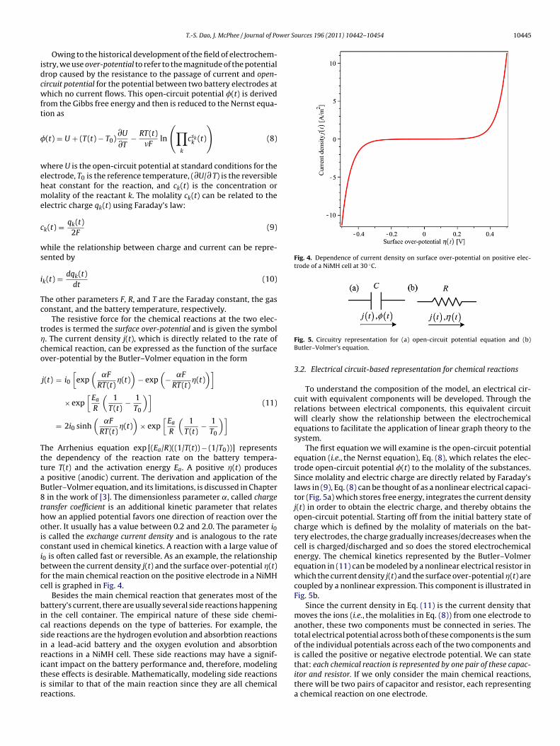

wer Sources 196 (2011) 10442– 10454 10445

idcwft

�

wehme

c

ws

i

Tc

t�co

TttaB8thoicibfc

bicsiritir

Fig. 4. Dependence of current density on surface over-potential on positive elec-trode of a NiMH cell at 30 ◦C.

T.-S. Dao, J. McPhee / Journal of Po

Owing to the historical development of the field of electrochem-stry, we use over-potential to refer to the magnitude of the potentialrop caused by the resistance to the passage of current and open-ircuit potential for the potential between two battery electrodes athich no current flows. This open-circuit potential �(t) is derived

rom the Gibbs free energy and then is reduced to the Nernst equa-ion as

(t) = U + (T(t) − T0)∂U

∂T− RT(t)

�Fln

(∏k

cskk (t)

)(8)

here U is the open-circuit potential at standard conditions for thelectrode, T0 is the reference temperature, (∂U/∂ T) is the reversibleeat constant for the reaction, and ck(t) is the concentration orolality of the reactant k. The molality ck(t) can be related to the

lectric charge qk(t) using Faraday’s law:

k(t) = qk(t)2F

(9)

hile the relationship between charge and current can be repre-ented by

k(t) = dqk(t)dt

(10)

he other parameters F, R, and T are the Faraday constant, the gasonstant, and the battery temperature, respectively.

The resistive force for the chemical reactions at the two elec-rodes is termed the surface over-potential and is given the symbol. The current density j(t), which is directly related to the rate ofhemical reaction, can be expressed as the function of the surfacever-potential by the Butler–Volmer equation in the form

j(t) = i0

[exp

(˛F

RT(t)�(t)

)− exp

(− ˛F

RT(t)�(t)

)]× exp

[Ea

R

(1

T(t)− 1

T0

)]= 2i0 sinh

(˛F

RT(t)�(t)

)× exp

[Ea

R

(1

T(t)− 1

T0

)] (11)

he Arrhenius equation exp [(Ea/R)((1/T(t)) − (1/T0))] representshe dependency of the reaction rate on the battery tempera-ure T(t) and the activation energy Ea. A positive �(t) produces

positive (anodic) current. The derivation and application of theutler–Volmer equation, and its limitations, is discussed in Chapter

in the work of [3]. The dimensionless parameter ˛, called chargeransfer coefficient is an additional kinetic parameter that relatesow an applied potential favors one direction of reaction over thether. It usually has a value between 0.2 and 2.0. The parameter i0s called the exchange current density and is analogous to the rateonstant used in chemical kinetics. A reaction with a large value of0 is often called fast or reversible. As an example, the relationshipetween the current density j(t) and the surface over-potential �(t)or the main chemical reaction on the positive electrode in a NiMHell is graphed in Fig. 4.

Besides the main chemical reaction that generates most of theattery’s current, there are usually several side reactions happening

n the cell container. The empirical nature of these side chemi-al reactions depends on the type of batteries. For example, theide reactions are the hydrogen evolution and absorbtion reactionsn a lead-acid battery and the oxygen evolution and absorbtioneactions in a NiMH cell. These side reactions may have a signif-

cant impact on the battery performance and, therefore, modelinghese effects is desirable. Mathematically, modeling side reactionss similar to that of the main reaction since they are all chemicaleactions.

Fig. 5. Circuitry representation for (a) open-circuit potential equation and (b)Butler–Volmer’s equation.

3.2. Electrical circuit-based representation for chemical reactions

To understand the composition of the model, an electrical cir-cuit with equivalent components will be developed. Through therelations between electrical components, this equivalent circuitwill clearly show the relationship between the electrochemicalequations to facilitate the application of linear graph theory to thesystem.

The first equation we will examine is the open-circuit potentialequation (i.e., the Nernst equation), Eq. (8), which relates the elec-trode open-circuit potential �(t) to the molality of the substances.Since molality and electric charge are directly related by Faraday’slaws in (9), Eq. (8) can be thought of as a nonlinear electrical capaci-tor (Fig. 5a) which stores free energy, integrates the current densityj(t) in order to obtain the electric charge, and thereby obtains theopen-circuit potential. Starting off from the initial battery state ofcharge which is defined by the molality of materials on the bat-tery electrodes, the charge gradually increases/decreases when thecell is charged/discharged and so does the stored electrochemicalenergy. The chemical kinetics represented by the Butler–Volmerequation in (11) can be modeled by a nonlinear electrical resistor inwhich the current density j(t) and the surface over-potential �(t) arecoupled by a nonlinear expression. This component is illustrated inFig. 5b.

Since the current density in Eq. (11) is the current density thatmoves the ions (i.e., the molalities in Eq. (8)) from one electrode toanother, these two components must be connected in series. Thetotal electrical potential across both of these components is the sumof the individual potentials across each of the two components andis called the positive or negative electrode potential. We can state

that: each chemical reaction is represented by one pair of these capac-itor and resistor. If we only consider the main chemical reactions,there will be two pairs of capacitor and resistor, each representinga chemical reaction on one electrode.

10446 T.-S. Dao, J. McPhee / Journal of Power S

rasi

j

wic

�

Ibp

tTRr

3

twiicrob

c

Ioca

two graphs in Fig. 8 are coupled by the temperature variable T(t)which appears in Eqs. (8) and (11).

For the thermal domain, the graph is simply a set of edges con-nected in parallel. The through and across variables for the thermaldomain are the time-derivative of entropy S(t) and the battery tem-

Fig. 6. Circuitry representation for multiple reactions.

Now let us consider an electrode at which there are n chemicaleactions (i.e., both main and side reactions). Since these reactionsre independent of each other, the total electrode current den-ity jtotal(t) is obtained by adding up the current densities of thendividual reactions. That is

total(t) = j1(t) + j2(t) + · · · + jn(t) = icell

Asurf. (12)

here Asurf is the surface area of the porous electrode and icells the current produced by the battery. The voltage across eachapacitor–resistor pair is also the same

C1 (t) + �R1 (t) = �C2 (t) + �R2 (t) = · · · = �Cn (t) + �Rn (t) (13)

t can be inferred from Eqs. (12) and (13) that the electrode cane represented by multiple capacitor–resistor pairs hooked up inarallel as shown in Fig. 6.

We can close the circuit by connecting the positive and negativeerminals to a current source or an external load as shown in Fig. 7.he external load could be a complete electric vehicle. In this figure,int is the internal resistance of the battery. For some batteries, thisesistance is very small and its effects can be ignored.

.3. Thermal effects

So far, we have presented the electrical circuit representation forhe chemical reactions in an electrochemical cell. The model thate consider assumes that the battery temperature is constant or,

n other words, the battery model we have investigated so far is ansothermal model. This assumption is generally acceptable for smallells where the applied current is not high. However, when the cur-ent intensity is high, as in the case of traction batteries for electricr hybrid electric vehicles, the effects of battery temperature canecome significant.

Application of energy balance [14,15] to the whole cell yields

pmcelldT(t)

dt= −hAcell(T(t) − Ta) + icell(t)vcell(t)

−n∑

k=1

jk(t)

(�k(t) − T(t)

∂Uk

∂T

)(14)

n this equation, cp is the heat capacity of the cell, mcell is the massf the cell, h is the external heat transfer coefficient, Acell is theell container external surface area, Ta is the ambient temperature,nd n is the number of chemical reactions. The right-hand side of

ources 196 (2011) 10442– 10454

the equation consists of three terms: the first term corresponds tothe heat exchange with the outside environment through the cellcontainer walls according to Newton’s law of cooling, the secondterm refers to the irreversible heat arisen from ohmic heating forthe whole cell, and the last term is the reversible entropic heatreleased or absorbed by the chemical reactions. Eq. (14) shows thatthe heat generation rate is equal to the sum of heat transferred outof the system and the heat stored in the system.

According to classical thermodynamics, Eq. (14) can be writtenas

dQ (t)dt

= dQ ext(t)dt

+ dQ irr(t)dt

+ dQ rev(t)dt

, (15)

in which dQ(t) = cpmcelldT(t) according to the definition of heatcapacity and (dQext(t)/dt) = − hAcell(T(t) − Ta) according to Newton’slaw of cooling. The last two terms, (dQ irr(t)/dt) = icell(t)vcell(t) and(dQ rev(t)/dt) = −

∑nk=1jk(t)(�k(t) − T(t)(∂Uk/∂T)), are the rates of

heat dissipated/absorbed due to the internal resistance and chem-ical reactions. In electrochemistry, Qrev(t) is also called the Gibbsfree-energy change.

In order to develop a linear graph for the thermal domain,we need to transform the thermal balance equation into thetemperature-entropy form so that the through S(t) and across T(t)variables appear explicitly in the equation. Dividing both sides ofEq. (15) by T(t) results in

S(t) = Sext(t) + Sirr(t) + Srev(t), (16)

where Sext(t), Sirr(t), and Srev(t) are the time derivatives of theentropy for the external temperature exchange term, the irre-versible term, and the reversible term, respectively. In Eq. (16),Srev(t) is the sum of the individual entropies for the chemical reac-tions and can be expressed as Srev(t) =

∑nk=1Srevk

(t).

3.4. Linear graph for battery model

Following the circuitry representation for the chemical domainas discussed in Section 3.2 and the temperature-entropy represen-tation given in Section 3.3, we can develop the linear graphs forboth domains. Examples for such graphs are shown in Fig. 8. In thisfigure, C’s and R’s are the nonlinear capacitors and resistors whoseequations are given in (8) and (11). For convenience, the currenti(t) and voltage v(t) will be used as through and across variables forthe chemical domain. The current flowing through each componentcan be related to the current density by i(t) = Asurfj(t). The voltageacross each resistor is the surface-over potential �(t) while the volt-age across the each capacitor component is the open-circuit voltage�(t). The tree branches and chords have been arbitrarily chosen asshown in Fig. 8a, which bears a striking resemblance to the physicalsystem in Fig. 7. We use a solid line to represent a tree branch and adotted line for a chord. If the model of the external circuit is known,we can also construct the linear graph for the entire system. For bat-tery charge and discharge operations, the external circuit is simplya current source which delivers electric current to the battery. The

perature T(t), respectively. It can be realized that the product of S(t)and T(t) is power, same as the product of voltage and current. Thisindicates that the energy flowing through the system componentsis conserved.

T.-S. Dao, J. McPhee / Journal of Power Sources 196 (2011) 10442– 10454 10447

Fig. 7. Equivalent circuit-based representation for electrochemical cell.

a) che

pa

i

av

q

v

Fig. 8. Linear graph representation for (

The system dynamic equations can be developed following therocedures discussed in Section 2.2. We can write the through vari-bles vector for the chemical domain as

=[

iCc1 (t) . . . iCan (t) iRc1 (t) . . . iRan (t) iRint(t) icell(t)

]T

(17)

The molalities ck’s in Eq. (8) can be replaced by charge vari-bles qk’s using Faraday’s law in (9). These charges are also throughariables

=[

qCc1 (t) . . . qCan (t) qRc1 (t) . . . qRan (t) qRint(t) qcell(t)

]T

(18)

Similarly, the across variable vector can be defined as follows

[ ]T

= vCc1 (t) . . . vCan (t) vRc1 (t) . . . vRan (t) vRint(t) vcell(t)

(19)

mical domain and (b) thermal domain.

We can also define the through and across variable vectors forthe thermal domain

s =[

Sext(t) Sirr(t) Srev1 (t) . . . Srevn (t) S(t)]T

(20)

and

t =[

Text(t) Tirr(t) Trev1 (t) . . . Trevn (t) T(t)]T

(21)

The branch and chord transformations can be applied directlyto the current and voltage variables as shown in Eqs. (4) and (3).However, for the charge variables, initial values, which appear aswe integrate the current variables, must be included in the chordtransformation equation. This gives

[qb(t) + qb(0)] = −Acq[qc(t) + qc(0)] (22)

The formulation procedures for an electrochemical system canbe summarized as in Fig. 9. The figure depicts the steps in the for-mulation as well as their resulting output variables. After the final

step we obtain 2(n − 1) + 1 ODEs representing the charge–currentrelation equations, 2(n − 1) + 1 algebraic equations for the chemi-cal domain, and 1 ODE for the thermal domain. It can be observedthat 2(n − 1) + 1 is also the number of chords in the linear graph.

10448 T.-S. Dao, J. McPhee / Journal of Power S

Tttccis

4

btarcd(bt

Fig. 9. Formulation steps for electrochemical cells.

he number of equations can be reduced further if some of thehrough variables are known functions of time. As an example, ifhe applied current on the battery terminals is known then icellan be considered as a current driver and two equations (i.e., oneharge–current relation and one algebraic equation) can be elim-nated from the final equations since the value of icell can now beubstituted directly into all the equations.

. Application to NiMH cell model

Due to its dominance in almost all hybrid vehicles the NiMHattery model has been chosen to demonstrate the technique inhis paper. The NiMH is one of the latest battery technologiesnd has many advantages over the other more commonly usedechargeable batteries such as the lead-acid battery or the nickel-admium battery. Some of these advantages include higher energy

ensity, more environmental friendly, and less prone to memoryi.e., periodic exercise cycles need to be done less often). The NiMHattery model presented is a modified version of the lumped bat-ery model proposed by Wu et al. [4]. In this section, the NiMH

ources 196 (2011) 10442– 10454

chemistry together with side reactions and thermal effects will bepresented, followed by a linear-graph-based formulation for bothchemical and thermal domains.

4.1. NiMH battery chemistry

The chemical reactions on the two electrodes of the battery canbe written as follows:

Main reaction on positive electrode:

NiOOH + H2O + e−discharge�

chargeNi(OH)2 + OH− (23)

Side reaction on positive electrode:

2OH− → 12

O2 + H2O + 2e− (24)

Main reaction on negative electrode:

MH + OH−discharge�

chargeM + H2O + e− (25)

Side reaction on negative electrode:

12

O2 + H2O + 2e− → 2OH− (26)

where the metal M in the negative electrode is an inter-metalliccompound, usually a rare earth compound. During charging, oxy-gen is generated at the nickel electrode and the gas is formed whenthe solubility limit in the electrolyte is reached. The oxygen is thentransported to the metal hydride electrode where it is reduced bythe recombined reaction (26). During discharge, the oxygen gen-eration reaction may occurs at low rates, at which the potential ofthe nickel electrode is higher than the equilibrium potential of theoxygen generation [16,17].

The electromotive force in the battery as defined by the open-circuit potentials (i.e., Nernst’s equations) for the main reactions(23) and (25) on the positive and negative electrodes is

�1(t) = U1 + (T(t) − T0)∂U1

∂T+ RT(t)

Fln

(cH+,max − cH+ (t)

cecH+ (t)

)(27)

�3(t) = U3 + (T(t) − T0)∂U3

∂T+ RT(t)

Fln(

c2e

)+ 9.712 × 10−4

+0.2372 exp

(−28.057cMH(t)

cMH,max

)

− 2.7302 × 10−4

(cMH(t)/cMH,max)2 + 0.010768

(28)

and the equilibrium potential for the oxygen reactions (24) and (26)is given by

�2(t) = U2 + (T(t) − T0)∂U2

∂T+ RT(t)

2Fln

(p0.5

O2(t)

c2e

)(29)

In these equations, cH+ (t) is the concentration of Ni(OH)2, cMH(t)is the concentration of the metal hydride (MH), pO2 is the par-tial pressure of oxygen gas, and T(t) is the battery temperature.Other parameters and constants are listed in Table B.1. Eq. (28) wascurve-fitted from the experimental data of a nickel/KOH/LaNi5 bat-tery using a nickel oxide positive electrode provided by Paxton and

Newman [1]. There is only one open-circuit potential equation (29)for the two side reactions (24) and (26) since side reactions are cou-pled together by the oxygen transport from the positive electrodeto the negative electrode.

T.-S. Dao, J. McPhee / Journal of Power Sources 196 (2011) 10442– 10454 10449

resen

tt

j

wTg

i

i

i

wc

l

j

w

i

b

i

i

Fig. 10. Circuitry rep

The rate of chemical reactions on each electrode is defined byhe Butler–Volmer equation which relates the current density jk(t)o the surface over-potential �k(t) by

k(t) = i0,k

[exp

(˛kF

RT(t)�k(t)

)− exp

(− ˛kF

RT(t)�k(t)

)](30)

here k = 1 . . . 3 for the first three chemical equations (23)–(25).he exchange current density i0,k for each chemical equation isiven by

0,1 = i0,1,ref

(cH+ (t)cH+,ref

)0.5(ce

ce,ref

)0.5(cH+,max − cH+ (t)

cH+,max − cH+,ref

)0.5

× exp[

Ea,1

R

(1

T(t)− 1

T0

)](31)

0,2 = i0,2,ref

(ce

ce,ref

)0.5(pO2 (t)pO2,ref

)0.5

exp[

Ea,2

R

(1

T(t)− 1

T0

)](32)

0,3 = i0,3,ref

(cMH(t)cMH,ref

)0.5(ce

ce,ref

)0.5(cMH,max − cMH(t)cMH,max − cMH,ref

)0.5

× exp[

Ea,3

R

(1

T(t)− 1

T0

)](33)

here i0,k,ref is the exchange current density at a reference reactantoncentration.

For the oxygen reduction reaction on the negative electrode, aimiting current equation is used for the rate of reaction

4(t) = − pO2 (t)pO2,ref

i0,4 (34)

here

0,4 = i0,4,ref exp[

Ea,4

R

(1

T(t)− 1

T0

)](35)

The battery current icell(t) can be calculated from the charge

alance equations on the electrodes given by

cell(t) = Aposaposlpos(j1(t) + j2(t)) (36)

cell(t) = −Aneganeglneg(j3(t) + j4(t)) (37)

tation for NiMH cell.

The mass balance of the nickel active material is given by

j1(t) = FdcH+ (t)

dt

LNi(OH)2

�Ni(OH)2lposapos

(38)

j3(t) = FdcMH(t)

dt

LMH

�MHlneganeg(39)

Aposaposlposj2(t) + Aneganeglnegj4(t) = FdpO2

(t)

dt

Vgas

RT(t)(40)

The battery temperature can be obtained from the energy bal-ance of the whole cell described by Eq. (14).

4.2. Linear graph representation for chemical domain

The application of the linear graph concept to the chemical reac-tions of the NiMH battery is a straightforward operation. The mainand side chemical reactions for the NiMH battery model shown inSection 4.1 can be represented by an equivalent electrical circuitas shown in Fig. 10. The open-circuit voltage equations (27), (29)and (28) can be represented by nonlinear electrical capacitors C1,C2, and C3. The relationship between the electrical potentials �kand concentrations in these equations is similar to the capacitiverelationship between voltage and charge in an electrical capacitor.

The nonlinear resistors R1, R2, and R3 are used to model theresistive relationship between the current density and over voltagein Eq. (30). The current density for the oxygen reduction reactionin Eq. (34) and the applied current at the battery terminals canbe represented by the current drivers i4(t) = I4 and icell(t) = Iapp. Forsimplicity, it is assumed that the battery is cycled with a constantcurrent Iapp. We also assume that the battery has thin electrodesand, therefore, we can ignore the influence of the battery internalresistance.

The linear graph for the chemical domain is shown in Fig. 11.We see that the topological graph structure comprises eight edges,to which we have assigned arbitrary sign directions. The number ofequations to be solved simultaneously can be reduced by selectinga tree and using a branch-chord formulation, as described in Section2. Choosing C1, C3, C3, R2, and R3 as branches and R1, I4, and Iapp as

chords can reduce the number of final equations as it will be shownthat the equations for I4 and Iapp are known (i.e., limiting current foroxygen reduction reaction and constant charge/discharge current).

The column matrix of through variables is:

10450 T.-S. Dao, J. McPhee / Journal of Power S

i

v

i

i

ca

q

q

c

a

v

Fig. 11. Linear graph presentation for main and side chemical reactions.

=[

iC1(t) iC2(t) iC3(t) iR2(t) iR3(t) iR1(t) i4(t) icell(t)]T

(41)

Vector i can be broken down into the branch through variableector ib and chord through variable vector ic as

b =[

iC1(t) iC2(t) iC3(t) iR2(t) iR3(t)]T

(42)

c =[

iR1(t) i4(t) icell(t)]T

(43)

Since the currents, which are the derivatives of the electricalharges, are through variables, the charges are also through vari-bles and can be written in vector forms as

b =[

qC1(t) qC2(t) qC3(t) qR2(t) qR3(t)]T

(44)

c =[

qR1(t) q4(t) qcell(t)]T

(45)

The current and charge variables are expressed in terms of theurrent densities and concentrations as follows

iR1(t) = Aposaposlposj1(t)iR2(t) = Aposaposlposj2(t)iR3(t) = Aneganeglnegj3(t)i4(t) = Aneganeglnegj4(t)

(46)

nd

qC1(t) = FAposLNi(OH)2

�Ni(OH)2

cH+ (t)

qC3(t) = FAnegLMH

�MHcMH(t)

qC2(t) + q4(t) = FVgas

RT(t)pO2 (t)

(47)

Similarly, the across variable vector can be defined as follows

=[

vC1(t) vC2(t) vC3(t) vR2(t) vR3(t) vR1(t) v4(t) vcell(t)]T

(48)

ources 196 (2011) 10442– 10454

vb =[

vC1(t) vC2(t) vC3(t) vR2(t) vR3(t)]T

(49)

vc =[

vR1(t) v4(t) vcell(t)]T

(50)

where the voltage variables are related to the battery electricalpotentials by

vCk(t) = �k(t)vRk(t) = �k(t) k = 1 . . . 3 (51)

For convenience, the Butler–Volmer equations are convertedinto the conductance form by applying the inverse hyperbolic oper-ation to Eqs. (30) as

vRk(t) = RT(t)˛kF

ln

⎡⎣ jk(t)

2i0,k+

√(jk(t)2i0,k

)2

+ 1

⎤⎦ k = 1 . . . 3

(52)

The expressions in Eqs. (27), (29), (28), (34) and (52) can bewritten as functions of currents, charges, and voltages using therelations in (46), (47) and (51); doing so, we obtain the followingset of six terminal equations

vC1(t) = U1 + (T(t) − T0)∂U1

∂T

+RT(t)F

ln

(cH+,maxFAposLNi(OH)2

− �Ni(OH)2qC1(t)

ce�Ni(OH)2qC1(t)

)vC2(t) = U2 + (T(t) − T0)

∂U2

∂T

+RT(t)2F

ln

(√((qC2(t) + q4(t))/(FVgas))RT(t)

c2e

)

vC3(t) = U3 + (T(t) − T0)∂U3

∂T+ RT(t)

Fln(

c2e

)+ 9.712 × 10−4

+0.2372 exp

[− 28.057�MH

FAnegLMHcMH,maxqC3(t)

]

− 2.7302 × 10−4[((�MH/(FAnegLMHcMH,max))qC3(t)

]2 + 0.010768

vR2(t) = RT(t)˛2F

ln

[iR2(t)

2i0,2Aposaposlpos

+

√(iR2(t)

2i0,2Aposaposlpos

)2

+ 1

⎤⎦

vR3(t) = RT(t)˛3F

ln

[iR3(t)

2i0,3Aneganeglneg

+

√(iR3(t)

2i0,3Aneganeglneg

)2

+ 1

⎤⎦

vR1(t) = RT(t)˛1F

ln

[iR1(t)

2i0,1Aposaposlpos

+

√(iR1(t)

2i0,1Aposaposlpos

)2

+ 1

⎤⎦

(53)

In a similar manner, the current driver in (34) can also be written

as

i4(t) = −qC2(t) + q4(t)pO2,refFVgas

RT(t)i0,4 (54)

wer S

gm

A

wt

⎛⎜⎜⎝

c

⎛⎜⎜⎝

f

B

ie

t

(

+ q4

1

⎤⎦+

0) −))

1(0)

+ 1

⎤⎦

T.-S. Dao, J. McPhee / Journal of Po

We now define the f-cutset and f-circuit matrices. For the graphiven in Fig. 11 and the given tree selection, the fundamental-cutsetatrix is obtained:

f =

⎡⎢⎢⎢⎢⎣

1 0 0 0 0 −1 0 00 1 0 0 0 1 0 −10 0 1 0 0 0 1 10 0 0 1 0 1 0 −10 0 0 0 1 0 1 1

⎤⎥⎥⎥⎥⎦ =

[1b Ac

](55)

hich can be used to write the chord transformation equation forhis system

iC1(t)iC2(t)iC3(t)iR2(t)iR3(t)

⎞⎟⎟⎠ = −

⎡⎢⎢⎢⎢⎣

−1 0 01 0 −10 1 11 0 −10 1 1

⎤⎥⎥⎥⎥⎦(

iR1(t)i4(t)

icell(t)

)(56)

For the charge variables, initial values must be included in thehord transformation equations, which yields

qC1(t) − qC1(0)qC2(t) − qC2(0)qC3(t) − qC3(0)qR2(t) − qR2(0)qR3(t) − qR3(0)

⎞⎟⎟⎠ = −

⎡⎢⎢⎢⎢⎣

−1 0 01 0 −10 1 11 0 −10 1 1

⎤⎥⎥⎥⎥⎦(

qR1(t) − qR1(0)q4(t) − q4(0)

qcell(t) − qcell(0)

)(57)

From the fundamental-cutset matrix, one can directly obtain theollowing fundamental-circuit matrix:

f =

⎡⎢⎣

1 −1 0 −1 0 1 0 00 0 −1 0 −1 0 1 00 1 −1 1 −1 0 0 1

⎤⎥⎦ =

[Bb 1c

](58)

n which each row corresponds to an equation along the edgesnclosing each circuit.

Similarly, making use of Eq. (4), the branch transformation forhe system can be written explicitly as

) ⎡1 −1 0 −1 0

⎤⎛ vC1⎞

⎧⎪⎪⎪⎪⎪⎪⎪⎪⎪⎪⎪⎪⎪⎪⎪⎪⎪⎪⎨⎪⎪⎪⎪⎪⎪⎪⎪⎪⎪⎪⎪⎪⎪⎪⎪⎪⎪⎩

−Aneganeglneg[qcell(t) + qC2(0) − qR1(t) + qR1(0) − qcell(0)FVgaspO2,ref

RT(t)˛1F

ln

⎡⎣ iR1(t)

2i0,1Aposaposlpos+

√(iR1(t)

2i0,1Aposaposlpos

)2

+

+RT(t)F

ln

(FAposLNi(OH)2

cH+,max − �Ni(OH)2(qR1(t) + qR1(

ce�Ni(OH)2(qR1(t) + qR1(0) − qC1(0

−U2 + (T(t) − T0)∂U2

∂T+ RT(t)

2Fln

(√RT(t)(−qR1(t) + qR

−RT(t)˛2F

ln

⎡⎣ −iR1(t) + icell(t)

2i0,2Aposaposlpos+

√(−iR1(t) + icell(t)2i0,2Aposaposlpos

)2

vR1v4

vcell

= −⎢⎣ 0 0 −1 0 −10 1 −1 1 −1

⎥⎦⎜⎜⎝ vC2vC3vR2vR3

⎟⎟⎠ (59)

ources 196 (2011) 10442– 10454 10451

Substituting Eq. (47) and the first equation in (59) into the ter-minal equations in (53) we obtain

RT(t)˛1F

ln

⎡⎣ iR1(t)

2i0,1Aposaposlpos+

√(iR1(t)

2i0,1Aposaposlpos

)2

+ 1

⎤⎦+

+U1 + (T(t) − T0)∂U1

∂T+ RT(t)

F

× ln

(FAposLNi(OH)2

cH+,max − �Ni(OH)2qC1(t)

ce�Ni(OH)2qC1(t)

)+

−U2 + (T(t) − T0)∂U2

∂T+ RT(t)

2Fln

(√RT(t)(qC2(t) + q4(t))

c2e

√FVgas

)+

−RT(t)˛2F

ln

⎡⎣ iR2(t)

2i0,2Aposaposlpos+

√(iR2(t)

2i0,2Aposaposlpos

)2

+ 1

⎤⎦ = 0

(60)

By applying the chord transformations in (56) and (57) to bothcurrent and charge variables in (54) and (60), we obtain the follow-ing set of two equations:

(t)]RT(t)i0,4 = i4(t)

U1 + (T(t) − T0)∂U1

∂T+

qC1(0)))

+

+ qcell(t) − qcell(0) + qC2(0) + q4(t))

c2e

√FVgas

)+

= 0

(61)

It should be noted from the above equation that icell(t) is the cur-rent applied on the battery terminals and, therefore, is completelyknown. We have the following relationships

iR1(t) = dqR1(t)dt

i4(t) = dq4(t)dt

icell(t) = dqcell(t)dt

(62)

Therefore, Eq. (61) become a set of two ordinary differential equa-tions (ODEs) which only consists of three unknowns qR1(t), q4(t),and T(t) and can easily be solved using a numerical integrator withproper initial conditions, if the temperature is known.

4.3. Linear graph for thermal domain

In Section 4.2 we have shown the steps to develop a linear graphand system equations for a NiMH model under the assumptionof constant battery temperature. In real automotive applications,studying the thermal effects of batteries is of particular impor-tance due to the large influence of battery temperature on thebattery and vehicle performance. Besides reducing battery effi-ciency, overheating a battery may even cause an explosion if thebattery temperature is not controlled. Due to these reasons, it is

desirable to also develop a linear graph for the thermal effects in acar battery.

To construct a linear graph for the thermal domain, we canmake use of the entropy–temperature relationship in Eq. (16) for

10452 T.-S. Dao, J. McPhee / Journal of Power Sources 196 (2011) 10442– 10454

tevatf

4

ittoipT

aFqpbI

theiithhar1vtethps

Fig. 13. Battery discharge at constant rates.

Fig. 14. Battery charge at constant rates.

Fig. 12. Linear graph representation for thermal domain.

he four chemical reactions. Considering the time-derivative of thentropies as through variables and the temperature as an acrossariable, we can construct the linear graph for the thermal domains shown in Fig. 12. By applying the branch and chord transforma-ions in Eqs. (59), (56) and (57), we can also convert Eq. (16) into aunction that is only dependent on T(t), qR1(t), and q4(t).

.4. Simulation results

The model developed has been used to simulate several scenar-os in order to observe its behaviors, particularly with regard tohermal effects. Table B.1 contains the model parameters used inhe simulations. These parameters were identified using homotopyptimization from a 3.4 A h NiMH battery produced by North Amer-can Battery Company (NABC) based on the reference parametersrovided in the work of [4]. The battery data was measured at A&Dechnology’s laboratory in Ann Arbor, Michigan, USA.

The battery voltage versus time for four different dischargend charge rates from 1 C (3.4 A) to 1/8 C (0.425 A) are shown inigs. 13 and 14 . As expected, the battery voltage drops/rises moreuickly as the discharge/charge current is increased. Fig. 15 com-ares the battery voltages obtained from simulation results andattery testing data at a constant charge and discharge rate of 1/5 C.t can be seen that these results are in good agreement.

The battery temperature during discharge and charge versusime is shown in Figs. 16 and 17 . It is assumed that the batteryas been cooled down to room temperature (25 ◦C) at the start ofach simulation. In these figures, the depletion of reactants resultsn high over-potential loss that causes a rapid cell temperaturencrease. Due to the temperature exchange with the environment,he battery temperature is flattened out at the end of the cycle. At aigh charge rate, due to the high ohmic and over-potential losses,igh charge potential is needed as expected. The cell heat gener-tion is also significant at high discharge currents for the sameeasons. This may cause the cell temperature to rise more than0 ◦C. At high-rate charge, the oxygen generation also increasesery quickly, contributing significantly to the increase in the cellemperature. However, during discharge, oxygen gas is only gen-rated at low currents. This explains the difference between the cell

emperatures in the two figures at the same rates, particularly at theigh rates. Battery temperature control is therefore very important,articularly in a battery electric vehicle or hybrid electric vehicleystem where the current intensity is usually very high.

Fig. 15. Simulated and experimental battery voltages at 1/5 C charge/discharge rate.

T.-S. Dao, J. McPhee / Journal of Power S

Fig. 16. Battery temperature rising from initial temperature 25 ◦C at constant dis-charge rates.

Fr

m(coMnf

5

fgeTlascl

rt

Appendix B. NiMH battery parameters used in simulations

See Tables B.1 and B.2 .

Table A.1Through and across variables.

Domain Through (unit) Across (unit)

Electrical Current Voltagei (A) v (V)

Mechanical translational Force Velocity�F (N) �v (m s−1)

Mechanical rotational Torque Angular velocity�� (N m) �ω (rad s−1)

Hydraulic Volume flow Pressure�v (m3 s−1) p (N m−2)

Thermal Entropy flow TemperaturedS/dt (W K−1) T (K)

Chemical Molar flow Chemical potentialdN/dt (mol s−1) (J mol−1)

Table B.1NiMH battery parameters.

Parameter Unit Symbol Value

Specific electrode area ofpositive electrode

cm2 cm−3 apos 4000.0

Specific electrode area ofnegative electrode

cm2 cm−3 aneg 3000.0

Surface area of positiveelectrode

cm2 Apos 175.0

Surface area of negativeelectrode

cm2 Aneg 100.0

Thickness of positive electrode cm lpos 3.3 × 10−2

Thickness of negative electrode cm lneg 2.8 × 10−2

Loading of nickel activematerial

g cm−2 LNi(OH)26.8 × 10−2

Loading of metal hydridematerial

g cm−2 LMH 1.13 × 10−1

Concentration of KOHelectrolyte

mol cm−3 ce 7.0 × 10−3

Reference concentration ofKOH electrolyte

mol cm−3 ce,ref 1.0 × 10−3

Maximum concentration ofNi(OH)2 in nickel activematerial

mol cm−3 cH+,max 3.7 × 10−2

Reference concentration of mol cm−3 cH+,ref 0.5cH+,max

ig. 17. Battery temperature rising from initial temperature 25 ◦C at constant chargeates.

One of the most noticeable results is that the linear graphodel simulates approximately 30% faster than the lumped model

i.e., all equations in [4] are stacked together) at all charge and dis-harge rates as summarized in Table B.2. The simulation times werebtained from a DellTMOptiPlex 2.9 GHz desktop computer usingaple dsolve function based on the default Runge–Kutta Fehlberg

umeric integrator with the same settings (abserr = relerr = 10−7)or both linear graph and lumped models.

. Conclusion

In this paper, we have presented a linear graph formulationor systematically generating a compact set of dynamic equationsoverning electrochemical systems. By carefully managing howquations are formed, a smaller set of expressions is obtained.his benefits symbolic implementation by reducing the size of theargest expression that needs to be handled by the computer, thusllowing for the analysis of more complicated systems. It was alsohown that the equations obtained using linear graph theoreti-al approach simulated approximately 30% faster than the original

umped model.

Since the interconnections between a system’s components areepresented by a linear graph, tree selection strategies can be usedo determine the modeling variables for the system. It is clear that

ources 196 (2011) 10442– 10454 10453

this flexibility can provide benefits during formulation as well assimulation.

This approach can be extended to modeling a more complexsystem such as a battery electric vehicle or a hybrid electric vehi-cle within which a battery model is an important part. This is apotential for future research since modeling individual parts ofa battery/hybrid electric vehicle has been done in the literature[9,12,18], but never before using linear graph theory.

Acknowledgements

Financial support for this research has been provided by the Nat-ural Sciences and Engineering Research Council of Canada (NSERC),Toyota, and Maplesoft.

Appendix A. Through and across variables for somephysical systems

See Table A.1.

Ni(OH)2 in nickel activematerial

Maximum concentration ofhydrogen in metal hydridematerial

mol cm−3 cMH,max 1.0 × 10−1

10454 T.-S. Dao, J. McPhee / Journal of Power Sources 196 (2011) 10442– 10454

Table B.1 (Continued)

Parameter Unit Symbol Value

Reference concentration ofhydrogen in metal hydridematerial

mol cm−3 cMH,ref 0.5cMH,max

Reference oxygen pressure atm pO2,ref 1.0Exchange current density of

reaction at referencereactant concentration forfirst reaction

A cm−2 i0,1,ref 15.1 × 10−4

Exchange current density ofreaction at referencereactant concentration forsecond reaction

A cm−2 i0,2,ref 2.0 × 10−4

Exchange current density ofreaction at referencereactant concentration forthird reaction

A cm−2 i0,3,ref 10.2 × 10−4

Exchange current density ofreaction at referencereactant concentration forfourth reaction

A cm−2 i0,4,ref 13.2 × 10−4

Activation energy for firstreaction

J mol−1 Ea,1 10.0 × 103

Activation energy for secondreaction

J mol−1 Ea,2 120.0 × 103

Activation energy for thirdreaction

J mol−1 Ea,3 10.0 × 103

Activation energy for fourthreaction

J mol−1 Ea,4 10.0 × 103

Reversible heat for firstreaction

V K−1 ∂U1/∂ T −1.35 × 10−3

Reversible heat for secondreaction

V K−1 ∂U2/∂ T −1.68 × 10−3

Reversible heat for thirdreaction

V K−1 ∂U3/∂ T −1.55 × 10−3

Reversible heat for fourthreaction

V K−1 ∂U4/∂ T −1.68 × 10−3

Charge transfer coefficient ˛1 0.5Charge transfer coefficient ˛2 1.0Charge transfer coefficient ˛3 0.5Open-circuit voltage V U1,c , U1,d 0.527, 0.458Open-circuit voltage V U2 0.4011Open-circuit voltage V U3 −0.8279Open-circuit voltage V U4 0.4011Gas volume in NiMH cell cm3 Vgas 1.0 × 10−1

Density of nickel activematerial

g cm−3 �Ni(OH)23.4

Density of metal hydride g cm−3 �MH 7.47Reference battery temperature K T0 303.15

Table B.2Average simulation time (in s) comparison between linear graph model and lumpedmodel.

Applied current Linear graph model Lumped model

Discharge 1 C 0.898 1.115Discharge 1/2 C 0.922 1.176Discharge 1/4 C 0.902 1.121Discharge 1/8 C 0.916 1.198Charge 1 C 0.904 1.128Charge 1/2 C 0.919 1.122Charge 1/4 C 0.918 1.124

[[[

[[

[

[

[

[

Charge 1/8 C 0.920 1.189

References

[1] B. Paxton, J. Newman, J. Electrochem. Soc. 144 (11) (1997) 3818–3831.[2] J. Newman, T. William, AIChE J. 21 (1) (1975) 25–41.[3] J. Newman, K.E. Thomas-Alyea, in: Electrochemical Systems, 3rd ed., John Wiley

& Sons Inc., 2004.[4] B. Wu, M. Mohammed, D. Brigham, R. Elder, R.E. White, J. Power Sources 101

(2) (2001) 149–157.[5] Z.M. Salameh, M.A. Casacca, W.A. Lynch, IEEE Trans. Energy Convers. 7 (1)

(1992) 93–98.[6] M. Chen, G.A. Rincon-Mora, IEEE Trans. Energy Convers. 21 (2) (2006) 504–511.[7] P.H. Roe, in: Networks and Systems, Addison-Wesley, 1966.[8] G. Andrews, H. Kesavan, Mech. Mach. Theory 10 (1) (1975) 57–75.[9] J. McPhee, C. Schmitke, S. Redmond, Math. Comput. Modell. Dynam. Syst. 10

(1) (2004) 1–23.10] J. McPhee, Nonlinear Dynam. 9 (1996) 73–90.11] J. McPhee, Mech. Mach. Theory 33 (6) (1998) 805–823.12] C. Schmitke, K. Morency, J. McPhee, J. Multi-body Dynam. Part K 222 (4) (2008)

339–352.13] M. Léger, J. McPhee, Multibody Syst. Dyn. 18 (2) (2007) 277–297.14] Z.H. Wang, W.B. Gu, C.Y. Wang, Proceedings of the 196th ECS Fall Meeting,

Honolulu, Hawaii, 1999.15] P.M. Gomadam, J.W. Weidner, R.E. White, J. Electrochem. Soc. 150 (10) (2003)

A1339–A1345.16] W.B. Gu, C.Y. Wang, S. Li, M.M. Geng, B.Y. Liaw, Electrochim. Acta 44 (1999)

4525–4541.17] P. Albertus, J. Christensen, J. Newman, J. Electrochem. Soc. 155 (1) (2008)

A48–A60.18] T.-S. Dao, A. Seaman, J. McPhee, Proceedings of the 5th Asian Conference on

Multibody Dynamics, 2010.