journal of process control - university of california, los...
TRANSCRIPT

EA
La
b
a
ARRAA
KMPPPT
1
tcb(swfncop(
to
if
0h
Journal of Process Control 24 (2014) 448–462
Contents lists available at ScienceDirect
Journal of Process Control
j our na l ho me pa g e: www.elsev ier .com/ locate / jprocont
conomic model predictive control of parabolic PDE systems:ddressing state estimation and computational efficiency
iangfeng Laoa, Matthew Ellisa, Panagiotis D. Christofidesa,b,∗
Department of Chemical and Biomolecular Engineering, University of California, Los Angeles, CA 90095-1592, USADepartment of Electrical Engineering, University of California, Los Angeles, CA 90095-1592, USA
r t i c l e i n f o
rticle history:eceived 22 October 2013eceived in revised form 12 January 2014ccepted 13 January 2014vailable online 21 February 2014
eywords:odel predictive control
rocess economicsartial differential equations (PDEs)
a b s t r a c t
In a previous work [20], an economic model predictive control (EMPC) system for parabolic partial dif-ferential equation (PDE) systems was proposed. Through operating the PDE system in a time-varyingfashion, the EMPC system demonstrated improved economic performance over steady-state operation.The EMPC system assumed the knowledge of the complete state spatial profile at each sampling period.From a practical point of view, measurements of the state variables are typically only available at afinite number of spatial positions. Additionally, the basis functions used to construct a reduced-ordermodel (ROM) for the EMPC system were derived using analytical sinusoidal/cosinusoidal eigenfunctions.However, constructing a ROM on the basis of historical data-based empirical eigenfunctions by applyingKarhunen-Loève expansion may be more computationally efficient. To address these issues, several EMPC
rocess controlransport-reaction processes
systems are formulated for both output feedback implementation and with ROMs based on analyticalsinusoidal/cosinusoidal eigenfunctions and empirical eigenfunctions. The EMPC systems are evaluatedusing a non-isothermal tubular reactor example, described by two nonlinear parabolic PDEs, where asecond-order reaction takes place. The model accuracy, computational time, input and state constraintsatisfaction, and closed-loop economic performance of the closed-loop tubular reactor under the differentEMPC systems are compared.
. Introduction
Model predictive control (MPC) is a popular optimal controlechnique that has gained widespread popularity within the pro-ess control industries. In the past decade, significant work haseen done on MPC of partial differential equation (PDE) systemse.g., [8–10,12,19,21,24,25]). To guide the PDE system to the desiredteady-state profile, conventional MPC systems are formulatedith the sum of squared differences between the state and inputs
rom their corresponding steady-state values. More recently, eco-omic model predictive control (EMPC) formulated with a generalost function accounting directly for the process economics, whichperates systems in a dynamically optimal fashion, has been pro-osed for systems described by ordinary differential equationsODEs) (e.g., [7,13,17,16,18]).
The significant challenge to applying the proposed EMPC sys-ems directly to PDE systems is deriving a finite-dimensionalrdinary differential equation (ODE) in time approximation of the
∗ Corresponding author at: Department of Chemical and Biomolecular Engineer-ng, University of California, Los Angeles, CA 90095-1592, USA. Tel.: +1 310 794 1015;ax: +1 310 206 4107.
E-mail address: [email protected] (P.D. Christofides).
959-1524/$ – see front matter © 2014 Elsevier Ltd. All rights reserved.ttp://dx.doi.org/10.1016/j.jprocont.2014.01.007
© 2014 Elsevier Ltd. All rights reserved.
PDE model. Specifically, the finite-dimensional model must accu-rately predict the spatiotemporal evolution of the system, while, beof sufficiently low order for computational efficiency. To produce amodel-based control scheme for parabolic PDEs, Galerkin’s methodbased on either analytical or empirical basis functions is typicallyapplied to the PDE model. In addition, utilizing approximate iner-tial manifolds (AIMs) (e.g., [6,11]), a system of finite-dimensionalODEs that accurately describe the dynamics of the dominant (slow)modes of the PDE system is derived for the synthesis of low-order controllers (e.g., [2] and the book [5]). Order reduction usingGalerkin’s method and analytical eigenfunctions was employed in[20] where we proposed an EMPC scheme for parabolic PDE sys-tems.
While, the EMPC system of [20] demonstrated improved closed-loop economics (greater production rate of the desired product oversteady-state operation), the EMPC system assumed the knowledgeof the complete state spatial profile at each sampling period. Inpractice, however, measurements of the PDE system may only beavailable at a finite number of points. Therefore, the formulationof an output feedback EMPC for parabolic PDE systems based on
measurements at a finite number of points should be considered.Additionally, the EMPC systems presented in [20] were devel-oped on the basis of low-order and high-order nonlinear ordinarydifferential equation (ODE) models derived through Galerkin’s

cess C
mlRtfesLpcbfrp
trtPciSnsaams
2
2
o
y
f
f
x
wxdfsogTt
u
wms
x
where �k is an eigenfunction corresponding to the k-th eigenvalue�k and �k is an adjoint eigenfunction of the operator A.
Assumption 1 below characterizes the class of parabolic PDEsconsidered in this work and states that the eigenspectrum of oper-ator A can be partitioned into a finite part consisting of m sloweigenvalues which are close to the imaginary axis and a stable infi-nite complement containing the remaining fast eigenvalues whichare far in the left-half of the complex plane, and that the separationbetween the slow and fast eigenvalues of A is large. We also notethat the large separation of slow and fast modes of the spatial opera-
L. Lao et al. / Journal of Pro
ethod using analytical basis functions. Considering the possibleimitation for using analytical basis functions and to improve theOM accuracy, empirical eigenfunctions as the basis functions forhe Galerkin’s method may be considered. The empirical eigen-unctions may be constructed by applying Karhunen-Loève (K-L)xpansion (e.g., [26,15]). By collecting an ensemble of the systemolution data from process historical data or simulation data, the K-
expansion method considers the presence of the dominant spatialatterns in the solution of the parabolic PDEs and results in a moreomprehensive and accurate ROM than a ROM based on analyticalasis functions. This data-based construction of the basis functionsor order reduction to PDE systems has been widely adopted in theecent years in the context of model-based control problems forarabolic PDE systems (e.g., [4,27,2,1,28,22]).
In this work, several EMPC systems are formulated and appliedo a non-isothermal tubular reactor where a second-order chemicaleaction takes place. First, an output feedback EMPC formula-ion is presented. Second, a reduced-order model (ROM) of theDEs is constructed on the basis of historical data-based empiri-al eigenfunctions by applying Karhunen-Loève expansion to usen the formulation of a computationally efficient EMPC system.everal EMPC systems each using a different ROM (i.e., differentumber of modes and derived from either using analytical sinu-oidal/cosinusoidal eigenfunctions or empirical eigenfunctions) arepplied to the non-isothermal tubular reactor example. The modelccuracy, computational time and closed-loop economic perfor-ance of the closed-loop tubular reactor under the different EMPC
ystems are compared and discussed.
. Preliminaries
.1. Parabolic PDEs
We consider quasi-linear parabolic PDEs with measured outputsf the form:
∂x
∂t= A
∂x
∂z+ B
∂2x
∂z2+ Wu(t) + f (x(z, t)) (1)
j(t) =∫ 1
0
cj(z)x(z, t)dz (2)
or j = 1, . . ., p, with the boundary conditions:
∂x
∂z
∣∣∣∣z=0
= g0x(0, t),∂x
∂z
∣∣∣∣z=1
= g1x(1, t) (3)
or t ∈ [0, ∞) and the initial condition:
(z, 0) = x0(z) (4)
here z ∈ [0, 1] is the spatial coordinate, t ∈ [0, ∞) is the time,′(z, t) = [x1(z, t)· · ·xnx (z, t)] is the vector of the state variables (x′
enotes the transpose of x), f (x(z, t)) denotes a nonlinear vectorunction, yj(t) is the j-th measured output, and cj(z) are knownmooth functions of z (j = 1, . . ., p) whose functional form dependsn the type of the measurement sensor. The notation A, B, W, g0 and1 is used to denote (constant) matrices of appropriate dimensions.he control input vector is denoted as u(t) ∈ R
nu and is subject tohe following constraints:
min ≤ u(t) ≤ umax (5)
here umin and umax are the lower and upper bound vectors of theanipulated input vector, u(t). Moreover, the system states are also
ubject to the following state constraints:
i,min ≤∫ 1
0
rxi(z)xi(z, t)dz ≤ xi,max, i = 1, . . ., nx (6)
ontrol 24 (2014) 448–462 449
where xi,min and xi,max are the lower and upper state constraint forthe i-th state, respectively. The function rxi
(z) ∈ L2(0, 1) where L2(0,1) is the space of measurable, square-integrable functions on theinterval [0, 1] is the state constraint distribution function.
2.2. Galerkin’s method
We first formulate the PDE system of Eqs. (1)–(4) as an infinitedimensional system in the Hilbert space H([0, 1]; R
nx ), with H beingthe space of measurable vector functions defined on [0, 1], withinner product and norm:
(ω1, ω2) =∫ 1
0
(ω1(z), ω2(z))Rnx dz,
‖ω1‖2 = (ω1, ω1)12
(7)
where ω1, ω2 are two elements of H([0, 1]; Rnx ) and the notation
( · , · )Rnx denotes the standard inner product in Rnx . The state func-
tion x(t) on the state-space H is defined as
x(t) = x(z, t), t > 0, 0 ≤ z ≤ 1, (8)
and the operator A is defined as
Ax = Adx
dz+ B
d2x
dz2, 0 ≤ z ≤ 1. (9)
and the measured output operator is defined as:
Cx(t) =[(c1( · ), x( · , t)), . . ., (cp( · ), x( · , t))
]′(10)
Then, the system of Eqs. (1)–(4) takes the following form:
x(t) = Ax(t) + Bu(t) + F(x(t)), x(0) = x0 (11)
y(t) = Cx(t) (12)
where x0 = x0(z), Bu(t) = Wu(t) and F(x(t)) is a nonlinear vectorfunction in the Hilbert space. The eigenvalue problem for A takesthe form
A�k = �k�k, k = 1, . . ., ∞ (13)
subject to
d�k
dz
∣∣∣z=0
= g0�k(0),d�k
dz
∣∣∣z=1
= g1�k(1) (14)
tor in parabolic PDEs ensures that a controller which exponentiallystabilizes the closed-loop ODE system, also stabilizes the closed-loop infinite-dimensional system [3]. This assumption is satisfiedby the majority of diffusion–convection–reaction processes [5].
450 L. Lao et al. / Journal of Process C
A
1
2
3
ifissop((
x
ta
wCde�gaAnetid
2
fliop
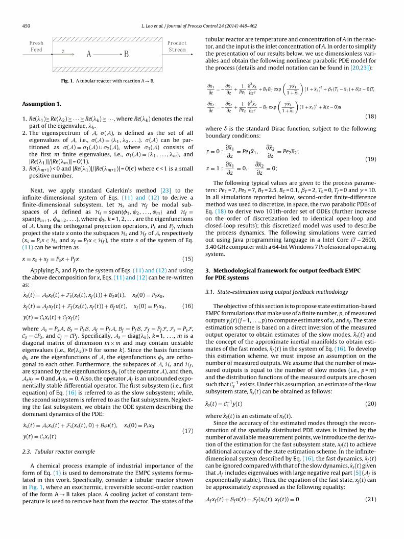
Fig. 1. A tubular reactor with reaction A → B.
ssumption 1.
. Re(�1)≥ Re(�2) ≥ · · · ≥ Re(�k) ≥ · · ·, where Re(�k) denotes the realpart of the eigenvalue, �k.
. The eigenspectrum of A, �(A), is defined as the set of alleigenvalues of A, i.e., �(A) = {�1, �2, . . .}. �(A) can be par-titioned as �(A) = �1(A) ∪ �2(A), where �1(A) consists ofthe first m finite eigenvalues, i.e., �1(A) = {�1, . . ., �m}, and|Re(�1)|/|Re(�m)| = O(1).
. Re(�m+1) < 0 and |Re(�1)|/|Re(�m+1)| = O(�) where � < 1 is a smallpositive number.
Next, we apply standard Galerkin’s method [23] to thenfinite-dimensional system of Eqs. (11) and (12) to derive anite-dimensional subsystem. Let Hs and Hf be modal sub-paces of A defined as Hs = span{�1, �2, . . ., �m} and Hf =pan{�m+1, �m+2, . . .}, where �k, k = 1, 2, . . . are the eigenfunctionsf A. Using the orthogonal projection operators, Ps and Pf, whichroject the state x onto the subspaces Hs and Hf of A, respectivelyxs = Psx ∈ Hs and xf = Pf x ∈ Hf ), the state x of the system of Eq.11) can be written as
= xs + xf = Psx + Pf x (15)
Applying Ps and Pf to the system of Eqs. (11) and (12) and usinghe above decomposition for x, Eqs. (11) and (12) can be re-writtens:
xs(t) = Asxs(t) + Fs(xs(t), xf (t)) + Bsu(t), xs(0) = Psx0,
xf (t) = Af xf (t) + Ff (xs(t), xf (t)) + Bf u(t), xf (0) = Pf x0,
y(t) = Csxs(t) + Cf xf (t)
(16)
here As = PsA, Bs = PsB, Af = Pf A, Bf = Pf B, Ff = Pf F, Fs = PsF,s = CPs, and Cf = CPf . Specifically, As = diag{�k}, k = 1, . . ., m is aiagonal matrix of dimension m × m and may contain unstableigenvalues (i.e., Re(�k) > 0 for some k). Since the basis functionsk are the eigenfunctions of A, the eigenfunctions �k are ortho-onal to each other. Furthermore, the subspaces of A, Hs and Hf ,re spanned by the eigenfunctions �k (of the operator A), and then,sxf ≡ 0 and Af xs ≡ 0. Also, the operator Af is an unbounded expo-entially stable differential operator. The first subsystem (i.e., firstquation) of Eq. (16) is referred to as the slow subsystem; while,he second subsystem is referred to as the fast subsystem. Neglect-ng the fast subsystem, we obtain the ODE system describing theominant dynamics of the PDE:
xs(t) = Asxs(t) + Fs(xs(t), 0) + Bsu(t), xs(0) = Psx0
y(t) = Csxs(t)(17)
.3. Tubular reactor example
A chemical process example of industrial importance of theorm of Eq. (1) is used to demonstrate the EMPC systems formu-
ated in this work. Specifically, consider a tubular reactor shownn Fig. 1, where an exothermic, irreversible second-order reactionf the form A → B takes place. A cooling jacket of constant tem-erature is used to remove heat from the reactor. The states of theontrol 24 (2014) 448–462
tubular reactor are temperature and concentration of A in the reac-tor, and the input is the inlet concentration of A. In order to simplifythe presentation of our results below, we use dimensionless vari-ables and obtain the following nonlinear parabolic PDE model forthe process (details and model notation can be found in [20,23]):
∂x1
∂t= − ∂x1
∂z+ 1
Pe1
∂2x1
∂z2+ BT BC exp
(�x1
1 + x1
)(1 + x2)2 + ˇT (Ts − x1) + ı(z − 0)Ti
∂x2
∂t= − ∂x2
∂z+ 1
Pe2
∂2x2
∂z2− BC exp
(�x1
1 + x1
)(1 + x2)2 + ı(z − 0)u
(18)
where ı is the standard Dirac function, subject to the followingboundary conditions:
z = 0 :∂x1
∂z= Pe1x1,
∂x2
∂z= Pe2x2;
z = 1 :∂x1
∂z= 0,
∂x2
∂z= 0;
(19)
The following typical values are given to the process parame-ters: Pe1 = 7, Pe2 = 7, BT = 2.5, BC = 0.1, ˇT = 2, Ts = 0, Tf = 0 and � = 10.In all simulations reported below, second-order finite-differencemethod was used to discretize, in space, the two parabolic PDEs ofEq. (18) to derive two 101th-order set of ODEs (further increaseon the order of discretization led to identical open-loop andclosed-loop results); this discretized model was used to describethe process dynamics. The following simulations were carriedout using Java programming language in a Intel Core i7 − 2600,3.40 GHz computer with a 64-bit Windows 7 Professional operatingsystem.
3. Methodological framework for output feedback EMPCfor PDE systems
3.1. State-estimation using output feedback methodology
The objective of this section is to propose state estimation-basedEMPC formulations that make use of a finite number, p, of measuredoutputs yj(t) (j = 1, . . ., p) to compute estimates of xs and xf. The stateestimation scheme is based on a direct inversion of the measuredoutput operator to obtain estimates of the slow modes, xs(t) andthe concept of the approximate inertial manifolds to obtain esti-mates of the fast modes, xf (t) in the system of Eq. (16). To developthis estimation scheme, we must impose an assumption on thenumber of measured outputs. We assume that the number of mea-sured outputs is equal to the number of slow modes (i.e., p = m)and the distribution functions of the measured outputs are chosensuch that C−1
s exists. Under this assumption, an estimate of the slowsubsystem state, xs(t) can be obtained as follows:
xs(t) = C−1s y(t) (20)
where xs(t) is an estimate of xs(t).Since the accuracy of the estimated modes through the recon-
struction of the spatially distributed PDE states is limited by thenumber of available measurement points, we introduce the deriva-tion of the estimation for the fast subsystem state, xf(t) to achieveadditional accuracy of the state estimation scheme. In the infinite-dimensional system described by Eq. (16), the fast dynamics, xf (t)can be ignored compared with that of the slow dynamics, xs(t) giventhat Af includes eigenvalues with large negative real part [5] (Af is
exponentially stable). Thus, the equation of the fast state, xf(t) canbe approximately expressed as the following equality:Af xf (t) + Bf u(t) + Ff (xs(t), xf (t)) = 0 (21)

cess C
nulxsE
Awe
x
RwTsCselsnmbmstlEtpelps
3f
tEnadfcfsf
u
s
x
x
x
u
x
x
L. Lao et al. / Journal of Pro
The fast state xf is equal to zero at its quasi-steady-state (weote that x(z, t) = 0 is a steady-state of the nominal PDE system(t) ≡ 0). Accounting for the fact that Af includes eigenvalues with
arge negative real parts, we can neglect the fast subsystem state,f(t) in the nonlinear term, Ff (xs, xf ). Using the estimated slow sub-ystem state, xs to calculate the approximate fast subsystem state,q. (21) becomes
f xf (t) + Bf u(t) + Ff (xs(t), 0) = 0 (22)
here xf (t) is the estimated fast state. An explicit form for thestimated fast state can be derived:
ˆf (t) = −A−1f
[Bf u(t) + Ff (xs(t), 0)] (23)
emark 1. The accuracy of the finite-dimensional ODE modelith m slow modes is of order � = |Re{�1(A)}|/|Re{�m+1(A)}| (O(�)).
his means under state feedback the closeness of the closed-loopystem PDE state to the closed-loop system ODE state is O(�).losed-loop stability under output feedback works not only for thelow and fast modes but also the real state as long as the estimationrror is negligible. This occurs when m is chosen to be sufficientlyarge such that � is sufficiently small. Specifically, to achieve theame level of closeness for the output feedback case (O(�)), theumber of measurements must be equal to the number of slowodes (i.e., p = m). From a practical standpoint, the discrepancy
etween the closed-loop PDE state under output feedback withore than m measurements and the one of the closed-loop PDE
tate under output feedback with m measurements will be indis-inguishable since the achieved closed-loop system performance isimited by the number of slow modes (m) used in the design of theMPC. Therefore, if there are more available measurement pointshan the slow modes (p > m), one can pick any m measurementoints from the set of p points as long as the assumption that C−1
s
xists is satisfied. In this work, from both the open-loop and closed-oop system simulation, we have good state estimation accuracy byicking m sufficiently large and choosing the measurement pointsuch that the inverse of the matrix Cs exists.
.2. Output feedback economic model predictive controlormulation
Utilizing the estimates xs and xf of Eqs. (20) and (23), respec-ively, we formulate a state estimation-based Lyapunov-basedMPC for the system of Eq. (16) to dynamically optimize an eco-omic cost function. We assume that the output measurementsre available continuously and synchronously at sampling instantsenoted as tk = k with k = 0, 1, . . .. Accounting for xf is importantor increasing PDE state estimation accuracy and satisfying stateonstraints. To formulate a finite-dimensional EMPC problem, theast subsystem is truncated at the l-th fast state. With the estimatedlow and fast modes, of Eqs. (20) and (23), respectively, the EMPCormulation takes the following form:
max∈S()
∫ ttk+N
tk
L(x(), u())d (24a)
.t. ˙xs(t) = Asxs(t) + Fs(xs(t), xf (t)) + Bsu(t) (24b)
˜s(tk) = C−1s y(tk) (24c)
˜f (t) = −A−1f
[Bf u(t) + ff (xs(t), 0)] (24d)
ˇ(t) = xs(t) + xf (t) (24e)
min ≤ u(t) ≤ umax, ∀t ∈ [tk, tk+N) (24f)
i,min ≤ (rxi, xi(t)) ≤ xi,max, i = 1, . . ., nx, ∀t ∈ [tk, tk+N) (24g)
ˇ ′(t)Px(t) ≤ � (24h)
ontrol 24 (2014) 448–462 451
where is the sampling period, S() is the family of piecewise con-stant functions with sampling period , N is the prediction horizon,xs(t) and xf (t) are the predicted evolution of the slow subsystemstate and fast subsystem state, respectively, with input u(t) com-puted by the EMPC and y(tk) is the output measurement at thesampling time tk.
In the optimization problem of Eq. (24), the objective functionof Eq. (24a) describes the dynamic economics of the process whichthe EMPC maximizes over a horizon tN. The constraint of Eq. (24b)is used to predict the future evolution of the slow subsystem withthe initial condition given in Eq. (24c) (i.e., the estimate of xs(tk)computed from the output y(tk)). The constraint of Eq. (24d) is thefinite-dimensional truncation of the fast subsystem which is usedto predict the evolution of the fast subsystem states. The symbolx(t) is used to denote the finite dimensional truncated state vec-tor (i.e., both the slow subsystem and the fast subsystem states).The constraints of Eqs. (24f)–(24g) are the available control actionand the state constraints, respectively. Finally, the constraint of Eq.(24h) ensures that the predicted state trajectory is restricted insidea predefined stability region which is a level set of the Lyapunovfunction (see [13] for a complete discussion of this issue). The opti-mal solution to this optimization problem is u * (t|tk) defined fort ∈ [tk, tk+N). The EMPC applies the control action computed for thefirst sampling period to the system in a sample-and-hold fashionfor t ∈ [tk, tk+1). The EMPC is resolved at the next sampling period,tk+1, after receiving a new output measurement, y(tk+1).
Remark 2. In the formulation of the state estimation-basedLyapunov-based EMPC of Eq. (24), Eq. (24h) defines a stabilityregion of the closed-loop system. This stability region is typicallycharacterized with an explicit stabilizing state feedback controller[13,14]. To account for the fact that additional uncertainty may beintroduced by using an output feedback controller over a state feed-back controller due to the estimation error, the stability region,computed using an explicit stabilizing state feedback controller,may be reduced for the output feedback case and a sufficiently largenumber of slow modes m (as well as number of output measure-ments p) can always be found to ensure that closed-loop stabilityunder output feedback is accomplished.
3.3. Implementation of output feedback EMPC
The output feedback EMPC is applied to the tubular reactor.To solve the EMPC problem, the open-source interior point solverIpopt [29] was used. Explicit Euler’s method was used with suffi-ciently small integration step of 1 × 10⁻⁴ to numerically integratethe finite-dimensional ODE model of the transport-reaction pro-cess. The cost function that we consider is to maximize the overallreaction rate along the length of the reactor. The economic cost thatthe EMPC works to maximize over the prediction horizon is
L(x, u) =∫ 1
0
r(z, t)dz (25)
where
r(z, t) = BC exp
(�x1
1 + x1
)(1 + x2)2 (26)
is the reaction rate.Regarding input and state constraints, the manipulated input
is subject to constraints as follows: −1 ≤ u ≤ 1. Owing to economicconsiderations, the amount of reactant material available over the
period tf is fixed. Specifically, the input trajectory should satisfy:1tf
∫ tf
0
u() d = 0.5 (27)

4 cess C
wtmat
x
fu
itmPpt.sx
y
w
y
Wmtwd
c
wzTC
t
x
wcta
t
y
52 L. Lao et al. / Journal of Pro
here tf = 1.0. To simplify the notation, we use the notation u ∈ g(tk)o denote this constraint. Constraints on the minimum and maxi-
um temperatures along the length of the reactor are considereds state constraints, Namely, the temperature along the length ofhe reactor must satisfy the following inequalities:
1,min ≤ x1(z, t) ≤ x1,max (28)
or all z ∈ [0, 1] where x1,min = −1 and x1,max = 3 are the lower andpper limits, respectively.
Since the PDE system of Eq. (18) consists of two PDEs, the index (i = 1, 2) is used to denote the i-th PDE of Eq. (18). We assumehe tubular reactor has p1 + p2 sensors where the first p1 sensors
easure the temperature (i.e., the state corresponding to the firstDE of Eq. (18)) at measurement points zs,1j ∈ [0, 1] for j = 1, 2, . . .,1, and the next p2 sensors measure the concentration of A (i.e.,he second state) at measurement points zs,2j ∈ [0, 1] for j = 1, 2,
. ., p2. Thus, the output measurements consist of the state mea-urements at a finite number of points in the spatial domain (i.e.,′i(tk) = [xi(zs,i1, tk)· · ·xi(zs,ipi
, tk)]) and can be written as
ij(tk) = xi(zs,ij, tk), i = 1, 2, j = 1, 2, . . ., pi
here the output measurement vector, y′(tk) = [y′1(tk)y′
2(tk)] and
′i(tk) = [yi1(tk)· · ·yipi
(tk)], i = 1, 2.
e assume the number of measurements satisfies pi = mi wherei refers to the number of total slow modes retained from the i-
h PDE in the construction of the model of Eq. (24b). Since point-ise measurements are considered, the following measurementistribution function is used:
ij(z) = ı(z − zs,ij), i = 1, 2, j = 1, 2, . . ., pi (29)
here ı is the standard Dirac function. Each measurement point,s,ij in the spatial domain is assumed to be at zs,ij = (j − 1)/(pi − 1).he choice of measurement points satisfies the assumption that−1s,i
exists.The state xi(z, t) can be decomposed into the sum of the ampli-
udes and the eigenfunctions of the first li eigenmodes:
i(z, t) ≈li∑
j=1
aij(t)�ij(z), i = 1, 2 (30)
here aij(t) and �ij(z) are the amplitude and eigenfunctions asso-
iated with the j-th eigenvalue of the spatial operator A. Utilizinghe decomposition of Eq. (30), the estimated slow mode vector,′s,i(tk) = [as,i1(tk)· · ·as,ipi(tk)] (recall that mi = pi) can be written in
he following form:
i(tk) = Cs,ixi(tk) = Cs,ias,i(tk)
=
⎛⎜⎜⎜⎜⎝
�i1(zs,i1) �i2(zs,i1) . . . �ip(zs,i1)
�i1(zs,i2) �i2(zs,i2) . . . �ip(zs,i2)
......
. . ....
�i1(zs,ipi) �i2(zs,ipi
) . . . �ip(zs,ipi)
⎞⎟⎟⎟⎟⎠
⎛⎜⎜⎜⎜⎝
as,i1(tk)
as,i2(tk)
...
as,ipi(tk)
⎞⎟⎟⎟⎟⎠ (31)
ontrol 24 (2014) 448–462
for i = 1, 2. The estimated slow modes are:
as,i(tk) = C−1s,i
yi(tk)
=
⎛⎜⎜⎜⎜⎝
�i1(zs,i1) �i2(zs,i1) . . . �ip(zs,i1)
�i1(zs,i2) �i2(zs,i2) . . . �ip(zs,i2)
......
. . ....
�i1(zs,ipi) �i2(zs,ipi
) . . . �ip(zs,ipi)
⎞⎟⎟⎟⎟⎠
−1 ⎛⎜⎜⎜⎜⎝
xi(zs,i1, tk)
xi(zs,i2, tk)
...
xi(zs,ipi, tk)
⎞⎟⎟⎟⎟⎠(32)
where as,i(tk) is an estimate of as,i(tk) from the output measure-ment, y(tk).
Since the decomposition of Eq. (30) provides a simplifiedmethod for describing the temporal evolution of the PDE system,the reduced-order model used in the EMPC (Eqs. (24b) and (24d)) iswritten in terms of the temporal evolution of the amplitudes of eacheigenmode. After applying the decomposition of Eq. (30) to Eq. (16),multiplying both sides by the adjoint eigenfunction, and making asimilar approximation as in Eq. (23), the resulting reduced-ordermodel has the following form (the · notation is dropped for sim-plicity of presentation):
as,i(t) = As,ias,i(t) + Fs,i(as(t), af (t)) + Bs,iu(t),
af,i(t) = A−1f,i
[Bf,iu(t) + Ff,i(as(t), af (t))
], i = 1, 2
y(t) = Cs,1as,1(t) + Cs,2as,2(t) + Cf,1af,1(t) + Cf,2af,2(t)
(33)
where as,i(t) = [as,i1(t) as,i2(t)· · ·as,imi(t)]′ with elements as,ij(t) ∈
R associated with the amplitudes of the j-th eigenmodes. The vectoraf,i(t) is a vector of similar structure to as,i(t) with elements associ-ated with the next mi + 1 to li eigenmodes. The vector as(t) and af(t)are defined as as(t) = [as,1(t)as,2(t)]′ and af(t) = [af,1(t)af,2(t)]′. Usingthis notation, the matrix As,i is defined as As,i = diag{�ij}, j = 1, . . ., mi(i.e., a diagonal mi × mi matrix where diagonal entries are equal to�ij and the indices j and i are used to denote the j-th eigenmode ofthe i-th PDE state) and the matrix Af,i is defined as Af,i = diag{�ij},j = mi + 1, . . ., li. Therefore, the quadratic Lyapunov function of Eq.(24h) is also written in terms of the amplitudes and has the form:
V(a(t)) = a′(t)Pa(t) (34)
where a(t) denotes a vector consisting of the amplitudes of allretained eigenmodes (i.e., both as(t) and af(t)) for each PDE, P isan (l1 + l2) × (l1 + l2) identity matrix and � = 3 is used in the formu-lations of the EMPC systems below.
3.3.1. Case 1: low-order output feedback EMPC systemIn this set of simulations, a low-order output feedback EMPC
system of the form of Eq. (24) (the fast modes are neglected) isformulated for the tubular reactor with the economic cost functionof Eq. (25), the input constraint of Eq. (27) and the state constraintof Eq. (28). The low-order output feedback EMPC is given by thefollowing optimization problem:
maxu∈S()
1N
∫ tk+N
tk
(∫ 1
0
r(z, )dz
)d (35a)
s.t. ˙as,i(t) = As,ias,i(t) + Fs,i(as(t), 0) + Bs,iu(t), i = 1, 2 (35b)
a (t ) = C−1y (t ), i = 1, 2 (35c)
s,i k s i k−1 ≤ u(t) ≤ 1, ∀t ∈ [tk, tk+N) (35d)
u(t) ∈ g(tk) (35e)

cess Control 24 (2014) 448–462 453
−
a
wtatltwoictm
1
2
wmstc
toTpmtpfttt
00.2
0.40.6
0.81
00.2
0.40.6
0.81
0
0.5
1
1.5
2
2.5
3
zt
x 1(z,t)
F
L. Lao et al. / Journal of Pro
1 ≤m1∑j=1
as,1j(t)�1j(z) ≤ 3 (35f)
˜ ′s(t)Pas(t) ≤ � (35g)
here the notation as denotes the predicted temporal evolution ofhe amplitudes of the slow modes, the prediction horizon is N = 3nd the sampling time is = 0.01. The constraint of Eq. (35e) ishe integral input constraint of Eq. (27) formulated for the samp-ing time tk on the basis of the material usage from t = 0 to t = tko ensure that the integral input constraint is satisfied over theindow tf = 1.0 (for simplicity of presentation, the beginning of the
perating window is denoted as t = 0). The tubular reactor is initial-zed with a transient state profile (i.e., not the steady-state profileorresponding to the steady-state input us = 0.5). For the reactor,wo EMPC systems are formulated with the following low-order
odel of the PDE system:
. The low-order model based on 11 slow modes only (i.e.,m1 = m2 = 11).
. The low-order model based on 21 slow modes only (i.e.,m1 = m2 = 21).
here the measured output points consists of the state measure-ents at m1 = 11 or m1 = 21 points which are evenly spaced in the
patial domain. Additionally, the reactor under uniform in time dis-ribution of the reactant material over tf = 1.0 is also considered foromparison purposes.
The closed-loop state profiles of the reactor over one periodf = 1.0 under the output feedback EMPC formulated with the low-rder model based on 21 slow modes is displayed in Figs. 2 and 3.he computed manipulated input profiles from the low-order out-ut feedback EMPC systems formulated based on 11 and 21 slowodes, respectively, over one period are shown in Fig. 4. From Fig. 4,
he output feedback EMPC system based on 21 slow modes com-utes a smoother manipulated input profile than that of the output
eedback EMPC system based on 11 slow modes. The maximumemperature profiles of the tubular reactor under the EMPC sys-ems are shown in Fig. 5. Since the temperature directly influenceshe reaction rate, the optimal operating strategy is to operate the1
00.2
0.40.6
0.81
−1
−0.8
−0.6
−0.4
−0.2
t
x 2(z,t)
ig. 3. Closed-loop profile of x2 of the tubular reactor under the low-order output feedba
Fig. 2. Closed-loop profile of x1 of the tubular reactor under the low-order outputfeedback EMPC system of Eq. (35) based on 21 slow modes over one operation period.
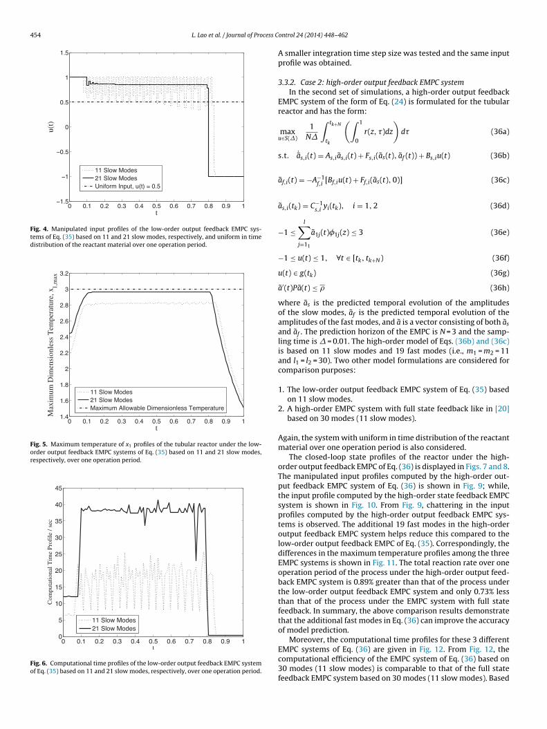
reactor at the maximum allowable temperature. From Fig. 5, bothEMPC systems operate the tubular reactor with a maximum tem-perature less than the maximum allowable which is a consequenceof the error associated with the low-order models. Since the low-order model based on 21 slow modes is able to more accuratelycompute the state profile, the output feedback EMPC system for-mulated with this low-order model operates the reactor at a greatertemperature than the other EMPC system.
Over one period tf = 1, the total reaction rate of the process underthe EMPC system based on 21 slow modes is 5.13% greater than thatof EMPC system based on 11 slow modes and 8.45% greater thanthat of the system under uniform in time distribution of the reactantmaterial. Moreover, the computational time profiles for these twoEMPC systems of Eq. (35) is given in Fig. 6. The EMPC system basedon 11 slow modes has a significant advantage in the computationalefficiency since it uses fewer modes in the reduced-order model.
Remark 3. Regarding the chattering in the computed input profile(Fig. 4), the chattering is not caused by the numerical integration.
00.2
0.40.6
0.8
z
ck EMPC system of Eq. (35) based on 21 slow modes over one operation period.
454 L. Lao et al. / Journal of Process C
0 0.1 0.2 0.3 0.4 0.5 0.6 0.7 0.8 0.9 1−1.5
−1
−0.5
0
0.5
1
1.5
t
u(t)
11 Slow Modes21 Slow ModesUniform Input, u(t) = 0.5
Fig. 4. Manipulated input profiles of the low-order output feedback EMPC sys-tems of Eq. (35) based on 11 and 21 slow modes, respectively, and uniform in timedistribution of the reactant material over one operation period.
0 0.1 0.2 0.3 0.4 0.5 0.6 0.7 0.8 0.9 11.4
1.6
1.8
2
2.2
2.4
2.6
2.8
3
3.2
t
Max
imum
Dim
ensi
onle
ss T
empe
ratu
re, x
1,m
ax
11 Slow Modes21 Slow ModesMaximum Allowable Dimensionless Temperature
Fig. 5. Maximum temperature of x1 profiles of the tubular reactor under the low-order output feedback EMPC systems of Eq. (35) based on 11 and 21 slow modes,respectively, over one operation period.
0 0.1 0.2 0.3 0.4 0.5 0.6 0.7 0.8 0.9 10
5
10
15
20
25
30
35
40
45
t
Com
puta
tiona
l Tim
e Pr
ofile
/ se
c
11 Slow Modes21 Slow Modes
Fig. 6. Computational time profiles of the low-order output feedback EMPC systemof Eq. (35) based on 11 and 21 slow modes, respectively, over one operation period.
ontrol 24 (2014) 448–462
A smaller integration time step size was tested and the same inputprofile was obtained.
3.3.2. Case 2: high-order output feedback EMPC systemIn the second set of simulations, a high-order output feedback
EMPC system of the form of Eq. (24) is formulated for the tubularreactor and has the form:
maxu∈S()
1N
∫ tk+N
tk
(∫ 1
0
r(z, )dz
)d (36a)
s.t. ˙as,i(t) = As,ias,i(t) + Fs,i(as(t), af (t)) + Bs,iu(t) (36b)
af,i(t) = −A−1f,i
[Bf,iu(t) + Ff,i(as(t), 0)] (36c)
as,i(tk) = C−1s,i
yi(tk), i = 1, 2 (36d)
−1 ≤l∑
j=11
a1j(t)�1j(z) ≤ 3 (36e)
−1 ≤ u(t) ≤ 1, ∀t ∈ [tk, tk+N) (36f)
u(t) ∈ g(tk) (36g)
a′(t)Pa(t) ≤ � (36h)
where as is the predicted temporal evolution of the amplitudesof the slow modes, af is the predicted temporal evolution of theamplitudes of the fast modes, and a is a vector consisting of both as
and af . The prediction horizon of the EMPC is N = 3 and the samp-ling time is = 0.01. The high-order model of Eqs. (36b) and (36c)is based on 11 slow modes and 19 fast modes (i.e., m1 = m2 = 11and l1 = l2 = 30). Two other model formulations are considered forcomparison purposes:
1. The low-order output feedback EMPC system of Eq. (35) basedon 11 slow modes.
2. A high-order EMPC system with full state feedback like in [20]based on 30 modes (11 slow modes).
Again, the system with uniform in time distribution of the reactantmaterial over one operation period is also considered.
The closed-loop state profiles of the reactor under the high-order output feedback EMPC of Eq. (36) is displayed in Figs. 7 and 8.The manipulated input profiles computed by the high-order out-put feedback EMPC system of Eq. (36) is shown in Fig. 9; while,the input profile computed by the high-order state feedback EMPCsystem is shown in Fig. 10. From Fig. 9, chattering in the inputprofiles computed by the high-order output feedback EMPC sys-tems is observed. The additional 19 fast modes in the high-orderoutput feedback EMPC system helps reduce this compared to thelow-order output feedback EMPC of Eq. (35). Correspondingly, thedifferences in the maximum temperature profiles among the threeEMPC systems is shown in Fig. 11. The total reaction rate over oneoperation period of the process under the high-order output feed-back EMPC system is 0.89% greater than that of the process underthe low-order output feedback EMPC system and only 0.73% lessthan that of the process under the EMPC system with full statefeedback. In summary, the above comparison results demonstratethat the additional fast modes in Eq. (36) can improve the accuracyof model prediction.
Moreover, the computational time profiles for these 3 different
EMPC systems of Eq. (36) are given in Fig. 12. From Fig. 12, thecomputational efficiency of the EMPC system of Eq. (36) based on30 modes (11 slow modes) is comparable to that of the full statefeedback EMPC system based on 30 modes (11 slow modes). Based
L. Lao et al. / Journal of Process Control 24 (2014) 448–462 455
00.2
0.40.6
0.81
00.2
0.40.6
0.81
0.5
1
1.5
2
2.5
3
zt
x 1(z,t)
Fig. 7. Closed-loop profile of x1 of the process under the high-order output feedbackEMPC system of Eq. (36) based on 30 modes (11 slow modes) over one operationperiod.
00.2
0.40.6
0.81
00.2
0.40.6
0.81
−1
−0.8
−0.6
−0.4
−0.2
zt
x 2(z,t)
Fig. 8. Closed-loop profile of x2 of the process under the high-order output feedbackEMPC system of Eq. (36) based on 30 modes (11 slow modes) over one operationperiod.
0 0.1 0.2 0.3 0.4 0.5 0.6 0.7 0.8 0.9 1−1.2
−0.8
−0.4
0
0.4
0.8
1.2
t
u(t)
30 Modes (11 Slow Modes, Output Feedback)Uniform Input, u(t) = 0.5
Fig. 9. Manipulated input profiles of the high-order output feedback EMPC systemof Eq. (36) based on 30 modes (11 slow modes) and uniform in time distribution ofthe reactant material over one operation period.
0 0.1 0.2 0.3 0.4 0.5 0.6 0.7 0.8 0.9 1−1.2
−0.8
−0.4
0
0.4
0.8
1.2
t
u(t)
30 Modes (11 Slow Modes, State Feedback)Uniform Input, u(t) = 0.5
Fig. 10. Manipulated input profiles of the high-order full state feedback EMPC sys-tem based on 30 modes (11 slow modes) and uniform in time distribution of thereactant material over one operation period.
0 0.1 0.2 0.3 0.4 0.5 0.6 0.7 0.8 0.9 1
1.6
1.8
2
2.2
2.4
2.6
2.8
3
3.2
t
Max
imum
Dim
ensi
onle
ss T
empe
ratu
re, x
1,m
ax
30 Modes (11 Slow Modes, Output Feedback)11 Modes (11 Slow Modes, Output Feedback)30 Modes (11 Slow Modes, State Feedback)Maximum Allowable Dimensionless Temperature
Fig. 11. Maximum temperature of x1, profiles of the low-order output feedbackEMPC system of Eq. (35) based on 11 slow modes, the high-order output feedbackEMPC system of Eq. (36) based on 30 modes (11 slow modes), the high-order fullstate feedback EMPC system based on 30 modes (11 slow modes) over one operationperiod.
0 0.1 0.2 0.3 0.4 0.5 0.6 0.7 0.8 0.9 10
10
20
30
40
50
60
70
t
Com
puta
tiona
l Tim
e Pr
ofile
/ se
c
30 Modes (11 Slow Modes, Output Feedback)11 Modes (11 Slow Modes, Output Feedback)30 Modes (11 Slow Modes, State Feedback)
Fig. 12. Computational time profiles of the low-order output feedback EMPC systemof Eq. (35) based on 11 slow modes, the high-order output feedback EMPC systemof Eq. (36) based on 30 modes (11 slow modes), the high-order full state feedbackEMPC system based on 30 modes (11 slow modes) over one operation period.

456 L. Lao et al. / Journal of Process Control 24 (2014) 448–462
0 0.1 0.2 0.3 0.4 0.5 0.6 0.7 0.8 0.9 1
−1
−0.5
0
0.5
1
t
u(t)
11 Slow Modes with White Noise on Output Measurement
Fig. 13. Manipulated input profiles of the low-order output feedback EMPC systemwith white noise on output measurements (solid line). The dotted line representsu
otmbE
3f
oocsibawtbttiomilcsitlrtmm
4e
fuls
0 0.1 0.2 0.3 0.4 0.5 0.6 0.7 0.8 0.9 1
1.7
1.9
2.1
2.3
2.5
2.7
2.9
3.1
3.3
t
Max
imum
Dim
ensi
onle
ss T
empe
ratu
re, x
1,m
ax
11 Slow Modes with White Noise on Output Measurement
Maximum Allowable Dimensionless Temperature
Fig. 14. Maximum temperature of x1 profile of the low-order output feedback EMPC
niform in time distribution of the reactant material over one operation period.
n the above results, from a practical point of view, comparableotal economic cost and computational time is achieved while using
uch fewer measurement points with the high-order output feed-ack EMPC system than that resulting from the full state feedbackMPC system.
.3.3. Case 3: measurement noise effect on low-order outputeedback EMPC system
In this case, the effect of bounded measurement noise on theutput measurements is considered. Process noise is added to eachf the output measurements (recall that the output measurementsonsist of point-wise measurements of each of the states along thepatial domain). The process noise is modeled as bounded Gauss-an white noise with 0 mean, unit variance, and bounds giveny −wmax,i ≤ wi ≤ wmax,i for i = 1, 2 where wi is the noise valuend wmax,i is the bound on the noise. The bounds are given bymax,1 = 0.1 and wmax,2 = 0.1 which corresponds to 3% and 5% of
he maximum state value, respectively. The low-order output feed-ack EMPC system based on 11 slow modes as in Case 1 is appliedo the tubular reactor. The closed-loop manipulated input profile ofhe reactor under the low-order output feedback EMPC is displayedn Fig. 13. Comparing Fig. 13 with the manipulated input profilef the low-order output feedback EMPC without output measure-ent noise in Fig. 4, the white noise causes increased chattering
n the computed input profile, but the EMPC still maintains closed-oop stability (i.e., boundedness of the closed-loop state profile in aompact set). The maximum temperature profile of the closed-loopystem with measurement noise under the EMPC system is shownn Fig. 14. The EMPC system can still maintain operation belowhe maximum allowable temperature. Furthermore, the closed-oop economic performance index (i.e., the integral of Eq. (25) withespect to time integrated over the operating window) is 4.37 forhe case without measurement noise and 4.32 for the case with
easurement noise (1.1% decrease in economic performance wheneasurement noise is added).
. Methodological framework for low-order EMPC usingmpirical eigenfunctions
As another way to derive a reduced-order model (ROM)
or the system of Eq. (11), empirical eigenfunctions may besed as basis functions in Galerkin’s method. This method canead to improved computational efficiency over using analyticalinusoidal/cosinusoidal eigenfunctions. In this section, the overall
system with white noise on output measurement and maximum allowable dimen-sionless temperature over one operation period.
approach is summarized followed by several closed-loop simu-lations of the closed-loop tubular reactor under an EMPC with amodel constructed from empirical eigenfunctions. Both state feed-back and output feedback implementation of the EMPC systemsformulated for the tubular reactor example are considered.
4.1. Implementation of Karhunen-Loève expansion
In order to compute the empirical eigenfunctions, we firstderive and solve a high-order and convergent discretization ofthe PDE of Eq. (18). In detail, 20 different initial conditions andarbitrary (constant) input values, u(t) were applied to the processmodel to get the spatiotemporal solution profiles. Consequently,from each simulation solution profile, 125 uniformly sampledsolutions (which are typically called “snapshots”) were takenand combined to generate an ensemble of 2500 solutions. TheKarhunen-Loève (K-L) expansion was applied to the developedensemble of solutions to compute empirical eigenfunctions thatdescribe the dominant spatial solution patterns embedded in theensemble where the Jacobian in the K-L expansion is calculatedthrough a finite-difference method. After truncating the eigenfunc-tions with relatively small eigenvalues (smaller than 1 × 10⁻⁵), wewere left with the first 4 eigenvalues which occupy more than99.99% of the total energy included in the entire ensemble. Thefirst 4 of these empirical eigenfunction profiles for each state arepresented in Figs. 15 and 16. Note that in contrast to the sinu-soidal/cosinusoidal eigenfunctions, these empirical eigenfunctionsare not symmetric with respect to the center of the spatial domainowing to the nonlinear term f and the input u(t).
The methodology used to carry out the order reduction andEMPC design is summarized below.
1. Initially, we form an ensemble of solutions of the PDE system ofEq. (1) for different values of manipulated input variables u(t).
2. Then, we apply Karhunen-Loève (K-L) expansion to this ensem-ble to derive a set of empirical eigenfunctions (dominant spatialpatterns that minimize the mean square error over all theensemble elements) [1].
3. The empirical eigenfunctions are used as basis functions within aGalerkin’s model reduction framework to transform the infinitedimensional nonlinear PDE system into a ROM in the form of a
low-dimensional nonlinear ODE system.4. Finally, an EMPC formulation is developed with the ROM andapplied to the tubular reactor example.

L. Lao et al. / Journal of Process Control 24 (2014) 448–462 457
0 0.2 0.4 0.6 0.8 1−2
−1.5
−1
−0.5
0
0.5
1
1.5
2
2.5
z
Em
piri
cal E
igen
func
tion
Set f
or x
11st Eigenfunction Profile2nd Eigenfunction Profile3rd Eigenfunction Profile4th Eigenfunction Profile
Fs
Rttrhatl�x�
4
ttmdimt
Fs
0 0.1 0.2 0.3 0.4 0.5 0.6 0.7 0.8 0.9 10
0.5
1
1.5
2
2.5
3
3.5
4
t
Stat
e D
iffe
renc
e N
orm
, ||d
X|| 2
8 Analytical Eigenfunctions7 Analytical Eigenfunctions4 Empirical Eigenfunctions3 Empirical Eigenfunctions
ig. 15. First 4 empirical eigenfunction set for x1 from an ensemble of 2500 systemolutions.
emark 4. As a practical implementation note, we point outhat even though the increase of the eigenfunctions appliedo the series expansion of Eq. (18) could improve the accu-acy of the computed approximate model, eigenfunctions thatave high frequency spatial profiles with small eigenvaluesre discarded because of the probable round off errors. Forhis case, the descending first 5 empirical eigenvalues areisted as follows: for x1(z, t), �1,1 = 2.365, �1,2 = 1.157 × 10−1,1,3 = 4.926 × 10⁻², �1,4 = 9.315 × 10⁻⁴, �1,5 = 7.255 × 10⁻⁶ and for2(z, t), �2,1 = 9.719 × 10⁻¹, �2,2 = 1.371 × 10⁻¹, �2,3 = 5.138 × 10−2,2,4 = 9.405 × 10⁻⁴, �2,5 = 8.930 × 10⁻⁶.
.2. Galerkin’s method with empirical eigenfunctions
To reduce the PDE model of Eq. (18) into an ODE model, weake advantage of the orthogonality of the empirical eigenfunc-ions obtained from the K-L expansion. Specifically, using Galerkin’s
ethod, we first derive a low-order ODE system for each of the PDEsescribing the temporal evolution of the amplitudes correspond-
ng to the first mi eigenfunctions. The low-order finite-dimensionalodel for the first j = 1, . . ., mi eigenfunctions of the i-th PDE has
he following form:
as,i(t) = As,ias,i(t) + Fs,i(as(t), 0) + Bs,iu(t), i = 1, 2 (37)
0 0.2 0.4 0.6 0.8 1−2.5
−2
−1.5
−1
−0.5
0
0.5
1
1.5
2
z
Em
piri
cal E
igen
func
tion
Set f
or x
2
1st Eigenfunction Profile2nd Eigenfunction Profile3rd Eigenfunction Profile4th Eigenfunction Profile
ig. 16. First 4 empirical eigenfunction set for x2 from an ensemble of 2500 systemolutions.
Fig. 17. L2 norm of the closed-loop evolution profiles of Eq. (18) using 4 differentROMs with respect to the evolution profile from the higher-order discretizationfinite difference method.
where a′s,i
(t) = [as,i1(t)· · ·as,imi(t)] is a vector of the amplitudes of
the first mi eigenfunctions.To present the effectiveness of empirical eigenfunctions in cap-
turing the dominant trends that appear during closed-loop processevolution, we let the process evolve starting from a certain initialcondition and under a constant input value, u(t) = 1. Four differentROMs are presented and compared to show the ROM accuracy in thecontext of EMPC handling manipulated input and state constraints.Specifically, the following ROMs are considered:
1. ROM using 8 analytical sinusoidal/cosinusoidal eigenfunctions(e.g., 8 eigenfunctions for each PDE state; 16 eigenfunctionstotal).
2. ROM using 7 analytical sinusoidal/cosinusoidal eigenfunctions.3. ROM using 4 empirical eigenfunctions.4. ROM using 3 empirical eigenfunctions.
We compared the square of the L2 norm, denoted as ||dX||2, toquantify the error of each of the reduced-order models. Specifically,we define ||dX||2 as
||dX||2 =2∑
i=1
101∑j=1
(xi,j − xi,j)2, i = 1, 2 (38)
where xi,j and xi,j are the state values of the i-th PDE at the j-th dis-crete points equally distributed along the spatial domain obtainedfrom reduced order model and the finite difference method, respec-tively. The four different reduced-order models are compared withrespect to the evolution profile from the higher-order discreti-zation finite difference method (i.e., the two 101th-order set ofODEs obtained by discretizing, in space, the two parabolic PDEsof Eq. (18)) under the same initial condition and input value inFig. 17. From the Fig. 17, comparing the L2 norm between theROM using 4 empirical eigenfunctions and the ROM using 8 ana-lytical eigenfunctions, the ROM constructed from the empiricaleigenfunctions is more accurate than the accuracy of the ROMconstructed from analytical eigenfunctions with more modes. Theaverage approximation error of each reduced-order model is atmaximum of the order of 10−1. Furthermore, we compared the
computational efficiency under the above two different modelreduction methods. The comparison of the computational timecorresponding to these 4 different ROMs is given in Fig. 18. TheROM based on empirical eigenfunctions shows its advantage on the
458 L. Lao et al. / Journal of Process Control 24 (2014) 448–462
0 0.1 0.2 0.3 0.4 0.5 0.6 0.7 0.8 0.9 1.0
0.12
0.16
0.2
0.24
0.28
t
Com
puta
tiona
l Tim
e / s
ec
8 Analytical Eigenfunctions7 Analytical Eigenfunctions4 Empirical Eigenfunctions3 Empirical Eigenfunctions
ca
4
oFdctf
4
uw
u
s
a
−
u
a
wta
foaolitc
0 0.1 0.2 0.3 0.4 0.5 0.6 0.7 0.8 0.9 1−1.5
−1
−0.5
0
0.5
1
1.5
t
u(t)
Fig. 19. Manipulated input profiles of the EMPC formulation of Eq. (39) using 4different ROMs over one operation period (profiles are overlapping).
Fig. 20. Closed-loop profile of x1 of the EMPC formulation of Eq. (39) using 4 differentROMs over one operation period (profiles are overlapping).
Fig. 18. Computational time profiles of Eq. (18) using 4 different ROMs.
omputational efficiency compared with the ROM based on thenalytical sinusoidal/cosinusoidal eigenfunctions.
.3. Implementation of EMPC
The implementations details of the EMPC are the same as for theutput feedback case (see Section 3.3) except for two differences.irst, the availability of the full state profile across the entire spatialomain is assumed at each sampling instance except for the thirdase study below, and second, the reduced-order model used inhe EMPC is constructed using empirical eigenfunctions as basisunctions.
.3.1. Case 1: low-order EMPC system with input constraints onlyIn this set of simulations, we consider an EMPC formulation
sing the model of Eq. (37) and considering only input constraintshich is of the form:
max∈S()
1N
∫ tk+N
tk
(∫ 1
0
r(z, )dz
)d (39a)
.t. ˙as,i(t) = As,ias,i(t) + Fs,i(as(t), 0) + Bs,iu(t) (39b)
˜s,ij(tk) = (�s,ij( · ), xi( · , tk)), j = 1, . . ., mi, i = 1, 2 (39c)
1 ≤ u(t) ≤ 1, ∀t ∈ [tk, tk+N) (39d)
∈ g(tk) (39e)
˜ ′s(t)Pas(t) ≤ � (39f)
here the notation is similar to the notation of the EMPC formula-ions in the previous sections. The EMPC of Eq. (39) is applied with
prediction horizon N = 2 and a sampling time = 0.01.The closed-loop behavior of the tubular reactor under an EMPC
ormulated with four different ROMs was considered: ROMs basedn 3 and 4 empirical eigenfunctions and ROMs based on 7 and 8nalytical sinusoidal/cosinusoidal eigenfunctions. For x(z, 0) = 0, allf these 4 ROMs achieve the same manipulated input and closed-oop state profiles under the EMPC of Eq. (39) which are shownn Figs. 19–21, respectively. We emphasize here on the compu-ational efficiency under the above two different methods. Theomparison of the computational time corresponding to these 4
Fig. 21. Closed-loop profile of x2 of the EMPC formulation of Eq. (39) using 4 differentROMs over one operation period (profiles are overlapping).
different situations is given in Fig. 22. The ROM based on empir-ical eigenfunctions shows its advantage on the computational
efficiency compared with the ROM based on the analytical sinu-soidal/cosinusoidal eigenfunctions.
L. Lao et al. / Journal of Process Control 24 (2014) 448–462 459
0 0.1 0.2 0.3 0.4 0.5 0.6 0.7 0.8 0.9 1.00
0.1
0.2
0.3
0.4
0.5
0.6
0.7
t
Com
puta
tiona
l Tim
e / s
ec
8 Analytical Eigenfunctions7 Analytical Eigenfunctions4 Empirical Eigenfunctions3 Empirical Eigenfunctions
Fd
4c
m
u
s
a
−
−u
a
Wtt
e1euu4aboci
rRtFEr
00.2
0.40.6
0.81
00.2
0.40.6
0.81
0.5
1
1.5
2
2.5
3
zt
x 1(z, t
)
Fig. 23. Closed-loop profile of x1 of EMPC formulation of Eq. (40) using the ROMbased on 4 empirical eigenfunctions over one operation period.
00.2
0.40.6
0.81
00.2
0.40.6
0.81
−1
−0.8
−0.6
−0.4
zt
x 2(z, t
)
Fig. 24. Closed-loop profile of x2 of EMPC formulation of Eq. (40) using the ROMbased on 4 empirical eigenfunctions over one operation period.
0 0.1 0.2 0.3 0.4 0.5 0.6 0.7 0.8 0.9 1
−1
−0.5
0
0.5
1
t
u(t)
4 Empirical Eigenfunctions8 Analytical Eigenfunctions12 Analytical EigenfunctionsUniform Input, u(t) = 0.5
ig. 22. Computational time profiles of the EMPC formulation of Eq. (39) using 4ifferent ROMs over one operation period.
.3.2. Case 2: low-order EMPC system with state and inputonstraints
In this case, the state constraint of Eq. (28) into the EMPC for-ulation and thus, the EMPC formulation takes the form:
max∈S()
1N
∫ tk+N
tk
(∫ 1
0
r(z, )dz
)d (40a)
.t. ˙as,i(t) = As,ias,i(t) + Fs,i(as(t), 0) + Bs,iu(t) (40b)
˜s,ij(tk) = (�s,ij( · ), xi( · , tk)), j = 1, . . ., mi, i = 1, 2 (40c)
1 ≤mi∑j=1
as,1j(t)�1j(z) ≤ 3 (40d)
1 ≤ u(t) ≤ 1, ∀t ∈ [tk, tk+N) (40e)
∈ g(tk) (40f)
˜ ′(t)Pa(t) ≤ � (40g)
e consider a prediction horizon N = 3 and a sampling time = 0.01. For this case, the initial condition is the steady-state of
he system under uniform input distribution, u = 0.5, as shown inhe Figs. 23 and 24.
We compared the simulation results from the ROM based on 4mpirical eigenfunctions (i.e., m1 = m2 = 4) and ROMs based on 8 and2 sinusoidal/cosinusoidal eigenfunctions, respectively, for x(z, 0)qual to the steady-state of the system under constant input value,(t) = 0.8. Figs. 23-24 show the closed-loop evolution of the statesnder the EMPC formulation of Eq. (40) from the ROM based on
empirical eigenfunctions. The manipulated input profiles for thebove 3 different ROMs are given in Fig. 25, which have the sameehavior as the ones in Case 1. For the input profile of ROM basedn 4 empirical eigenfunctions in Fig. 25 (solid line), the chattering isaused by the over-estimated maximum temperature by the ROMn EMPC, which is also seen in Fig. 26 (solid line).
For this case study, we compared the integral of the reactionate along the length of the reactor among the above 3 differentOMs and the case of the system under uniform in time distribu-
ion of the reactant material, i.e., u(t) = 0.5, as shown in Fig. 27. Fromig. 27, for the cases of 3 different ROMs, the reaction rates under theMPC significantly increase initially because of the second-ordereaction rate dependence. The economic cost decrease since theFig. 25. Manipulated input profiles of the EMPC formulation of Eq. (40) using 3different ROMs and uniform in time distribution of the reactant material profileover one operation period.
reactant material fed to the reactor decreases to satisfy the reac-
tant material constraint. Over tf, the total reaction rate from thesystem under the EMPC formulation from the ROM on the basisof 4 empirical eigenfunctions is 11.25% greater than that from the
460 L. Lao et al. / Journal of Process Control 24 (2014) 448–462
0 0.1 0.2 0.3 0.4 0.5 0.6 0.7 0.8 0.9 12
2.2
2.4
2.6
2.8
3
3.2
t
Max
imum
Dim
ensi
onle
ss T
empe
ratu
re, x
1,m
ax
4 Empirical Eigenfunctions8 Analytical Eigenfunctions12 Analytical EigenfunctionsMaximum Allowable Dimensionless Temperature
Fig. 26. Maximum temperature of x1 profiles of the EMPC formulation of Eq. (40)using 3 different ROMs over one operation period.
0 0.1 0.2 0.3 0.4 0.5 0.6 0.7 0.8 0.9 10
0.5
1
1.5
2
2.5
3
3.5
4
4.5
5
5.5
6
t
Rea
ctio
n R
ate,
L(x
,u)
4 Empirical Eigenfunctions8 Analytical Eigenfunctions12 Analytical EigenfunctionsUniform Input, u(t) = 0.5
Fru
sretcfit
EFab
4a
situoe
0 0.1 0.2 0.3 0.4 0.5 0.6 0.7 0.8 0.9 10
5
10
15
20
25
30
35
40
t
Com
puta
tiona
l Tim
e / s
ec
4 Empirical Eigenfunctions8 Analytical Eigenfunctions12 Analytical Eigenfunctions
Fig. 28. Computational time profiles of the EMPC formulation of Eq. (40) using 3different ROMs over one operation period.
00.2
0.40.6
0.81
00.2
0.40.6
0.81
0.5
1
1.5
2
2.5
3
zt
x 1(z,t)
ig. 27. The integral of the reaction rate along the length of the reactor of the tubulareactor under the EMPC formulation of Eq. (40) using 3 different ROMs and underniform in time distribution of the reactant material over one operation period.
ystem under uniform in time distribution of the reactant mate-ial. The total economic cost of the ROM on the basis of 4 empiricaligenfunctions is 0.79% and 1.85% greater than that of the ROM onhe basis of 8 and 12 analytical eigenfunctions, respectively. Thisan be explained from the point of view that the empirical eigen-unctions capture more information on the nonlinear terms and thenput effect in the original PDE model which is not considered byhe analytical eigenfunctions.
The comparison of the computational time corresponding to theMPC systems based on the above 3 different ROMs is given inig. 28. The ROM based on 4 empirical eigenfunctions shows itsdvantage on the computational efficiency compared with the ROMased on both 8 and 12 analytical eigenfunctions.
.3.3. Case 3: low-order output feedback EMPC system with statend input constraints
In this set of simulations, a low-order output feedback EMPCystem (Eq. (35)) based on a ROM using empirical eigenfunctionss formulated and applied to the tubular reactor. The tubular reac-
or is initialized with x(z, 0) equal to the steady-state of the systemnder constant input value, u(t) = 0.6. For the reactor, the low-orderutput feedback EMPC system based on the ROM using 4 empiricaligenfunctions is compared with the low-order output feedbackFig. 29. Closed-loop profile of x1 of EMPC formulation of Eq. (35) using the ROMbased on 4 empirical eigenfunctions over one operation period.
EMPC system based on 11 slow modes only (i.e., m1 = m2 = 11).Additionally, the reactor under uniform in time distribution of thereactant material over tf = 1.0 is also considered for comparisonpurposes.
We compared the simulation results from the low-orderoutput feedback EMPCs using the ROM based on 4 empiricaleigenfunctions (i.e., m1 = m2 = 4) and ROMs based on 11 sinu-soidal/cosinusoidal eigenfunctions, respectively. Figs. 29-30 showthe closed-loop evolution of the states under the EMPC formula-tion of Eq. (35) from the ROM based on 4 empirical eigenfunctions.The manipulated input profiles for the above 2 different ROMs aregiven in Fig. 31. For the input profile of ROM based on 4 empiricaleigenfunctions in Fig. 31 (solid line), the chattering is caused bythe over-estimated maximum temperature by the ROM in EMPC,which is also seen in Fig. 32 (solid line). Different from the simu-lation results in Section 4.3.2, the EMPC using the ROM based on4 empirical eigenfunctions has higher amplitude of fluctuation onthe input profile and also a much lower maximum temperaturein the reactor. This difference results from the limited number ofmeasurement points used with the EMPC using the ROM based on4 empirical eigenfunctions (i.e., p1 = p2 = m1 = m2 = 4) compared to
the EMPC using the ROM based on 11 analytical eigenfunctions (i.e.,p1 = p2 = m1 = m2 = 11).For this case study, we also compared the integral of the reac-tion rate along the length of the reactor among the above 2 different

L. Lao et al. / Journal of Process Control 24 (2014) 448–462 461
00.2
0.40.6
0.81
00.2
0.40.6
0.81
−1
−0.8
−0.6
−0.4
−0.2
zt
x 2(z,t)
Fig. 30. Closed-loop profile of x2 of EMPC formulation of Eq. (35) using the ROMbased on 4 empirical eigenfunctions over one operation period.
0 0.1 0.2 0.3 0.4 0.5 0.6 0.7 0.8 0.9 1−2
−1.5
−1
−0.5
0
0.5
1
1.5
t
u(t)
Output Feedback EMPC Using 4 Empirical Eigenfunctions Output Feedback EMPC Using 12 Analytical Eigenfunctions Uniform Input, u(t) = 0.5
Fig. 31. Manipulated input profiles of the EMPC formulation of Eq. (35) using theROM based on 4 empirical eigenfunctions and the ROM based on 11 analytical eigen-functions and uniform in time distribution of the reactant material profile over oneoperation period.
0 0.1 0.2 0.3 0.4 0.5 0.6 0.7 0.8 0.9 1
1.6
1.8
2
2.2
2.4
2.6
2.8
3
3.2
t
Max
imum
Dim
ensi
onle
ss T
empe
ratu
re, x
1,m
ax
Output Feedback EMPC Using 4 Empirical EigenfunctionsOutput Feedback EMPC Using 11 Analytical EigenfunctionsMaximum Allowable Dimensionless Temperature
Fig. 32. Maximum temperature of x1 profiles of the EMPC formulation of Eq. (35)using the ROM based on 4 empirical eigenfunctions and the ROM based on 11 analyt-ical eigenfunctions and maximum allowable dimensionless temperature over oneoperation period.
0 0.1 0.2 0.3 0.4 0.5 0.6 0.7 0.8 0.9 10
1
2
3
4
5
6
t
Rea
ctio
n R
ate,
L(x
,u)
Output Feedback EMPC Using4 Empirical EigenfunctionsOutput Feedback EMPC Using11 Analytical EigenfunctionsUniform Input, u(t) = 0.5
Fig. 33. The integral of the reaction rate along the length of the tubular reactor underthe EMPC formulation of Eq. (35) using the ROM based on 4 empirical eigenfunctions
and the ROM based on 11 analytical eigenfunctions and uniform in time distributionof the reactant material profile over one operation period.ROMs and the case of the system under uniform in time distribu-tion of the reactant material, i.e., u(t) = 0.5, as shown in Fig. 33. FromFig. 33, the total reaction rate over tf from the system under theEMPC formulation from the ROM on the basis of 4 empirical eigen-functions is still 9.45% greater than that from the system underuniform in time distribution of the reactant material and mean-while, 1.46% less than that of the ROM on the basis of 11 analyticaleigenfunctions.
5. Conclusions
In this work, two types of EMPC systems for quasi-linear PDEsystems were presented: (1) an output feedback EMPC systemand (2) an EMPC system formulated with a reduced-order modelderived using empirical eigenfunctions as basis functions. TheEMPC systems were applied to a tubular reactor of industrialimportance. Through time-varying operation, the EMPC systemsyielded improved closed-loop economic performance over steady-state operation. Additionally, constructing a ROM on the basisof historical data-based empirical eigenfunctions by applyingKarhunen-Loève expansion demonstrated computational bene-fits over using analytical sinusoidal/cosinusoidal eigenfunctions asbasis functions.
Acknowledgments
Financial support from the National Science Foundation and theDepartment of Energy is gratefully acknowledged.
References
[1] A. Armaou, P.D. Christofides, Dynamic optimization of dissipative PDE sys-tems using nonlinear order reduction, Chemical Engineering Science 57 (2002)5083–5114.
[2] J. Baker, P.D. Christofides, Finite-dimensional approximation and control ofnon-linear parabolic PDE systems, International Journal of Control 73 (2000)439–456.
[3] M.J. Balas, Feedback control of linear diffusion processes, International Journalof Control 29 (1979) 523–534.
[4] S. Banerjee, J.V. Cole, K.F. Jensen, Nonlinear model reduction strategies for rapid
thermal processing systems, IEEE Transactions on Semiconductor Manufactur-ing 11 (1998) 266–275.[5] P.D. Christofides, Nonlinear and Robust Control of PDE Systems: Methods andApplications to Transport-Reaction Processes, Birkhäuser, Boston, 2001.

4 cess C
[
[
[
[
[
[
[
[
[
[
[
[
[
[[
[
[
[
[
62 L. Lao et al. / Journal of Pro
[6] P.D. Christofides, P. Daoutidis, Finite-dimensional control of parabolic PDE sys-tems using approximate inertial manifolds, Journal of Mathematical Analysisand Applications 216 (1997) 398–420.
[7] M. Diehl, R. Amrit, J.B. Rawlings, A Lyapunov function for economic optimizingmodel predictive control, IEEE Transactions on Automatic Control 56 (2011)703–707.
[8] S. Dubljevic, P.D. Christofides, Predictive output feedback control of parabolicpartial differential equations (PDEs), Industrial & Engineering ChemistryResearch 45 (2006) 8421–8429.
[9] S. Dubljevic, N.H. El-Farra, P. Mhaskar, P.D. Christofides, Predictive controlof parabolic PDEs with state and control constraints, International Journal ofRobust and Nonlinear Control 16 (2006) 749–772.
10] S. Dubljevic, P. Mhaskar, N.H. El-Farra, P.D. Christofides, Predictive control oftransport-reaction processes, Computers & Chemical Engineering 29 (2005)2335–2345.
11] C. Foias, M.S. Jolly, I.G. Kevrekidis, G.R. Sell, E.S. Titi, On the computation ofinertial manifolds, Physics Letters A 131 (1988) 433–436.
12] D. Georges, Infinite-dimensional nonlinear predictive controller design foropen-channel hydraulic systems, in: Workshop on Irrigation Channels andRelated Problems, vol. 4, Maiori, Salerno, Italy, 2009, pp. 267–285.
13] M. Heidarinejad, J. Liu, P.D. Christofides, Economic model predictive control ofnonlinear process systems using Lyapunov techniques, AIChE Journal 58 (2012)855–870.
14] M. Heidarinejad, J. Liu, P.D. Christofides, State-estimation-based economicmodel predictive control of nonlinear systems, Systems & Control Letters 61(2012) 926–935.
15] P. Holmes, J.L. Lumley, G. Berkooz, Turbulence, Coherent Structures, Dynami-cal Systems and Symmetry, Cambridge University Press, New York, New York,1996.
16] R. Huang, L.T. Biegler, E. Harinath, Robust stability of economically orientedinfinite horizon NMPC that include cyclic processes, Journal of Process Control22 (2012) 51–59.
17] R. Huang, E. Harinath, L.T. Biegler, Lyapunov stability of economically orientedNMPC for cyclic processes, Journal of Process Control 21 (2011) 501–509.
[
ontrol 24 (2014) 448–462
18] R. Huang, S.C. Patwardhan, L.T. Biegler, Robust stability of nonlinear modelpredictive control based on extended Kalman filter, Journal of Process Control22 (2012) 82–89.
19] K. Ito, K. Kunisch, Receding horizon optimal control for infinite dimensionalsystems, ESAIM: Control, Optimisation and Calculus of Variations 8 (2002)741–760.
20] L. Lao, M. Ellis, P.D. Christofides, Economic model predictive control oftransport-reaction processes, Industrial & Engineering Chemistry Research(2014), http://dx.doi.org/10.1021/ie401016a, in press.
21] T.V. Pham, D. Georges, G. Besanc on, Receding horizon boundary control ofnonlinear conservation laws with shock avoidance, Automatica 48 (2012)2244–2251.
22] S. Pitchaiah, A. Armaou, Output feedback control of distributed parametersystems using adaptive proper orthogonal decomposition, Industrial & Engi-neering Chemistry Research 49 (2010) 10496–10509.
23] W.H. Ray, Advanced Process Control, McGraw-Hill, New York, New York, 1981.24] H. Shang, J.F. Forbes, M. Guay, Model predictive control for quasilinear hyper-
bolic distributed parameter systems, Industrial & Engineering ChemistryResearch 43 (2004) 2140–2149.
25] H. Shang, J.F. Forbes, M. Guay, Computationally efficient model predictive con-trol for convection dominated parabolic systems, Journal of Process Control 17(2007) 379–386.
26] L. Sirovich, Turbulence and the dynamics of coherent structures, I – Coherentstructures. II – Symmetries and transformations. III – Dynamics and scaling,Quarterly of Applied Mathematics 45 (1987) 561–590.
27] A. Theodoropoulou, R.A. Adomaitis, E. Zafiriou, Model reduction for optimiza-tion of rapid thermal chemical vapor deposition systems, IEEE Transactions onSemiconductor Manufacturing 11 (1998) 85–98.
28] A. Varshney, S. Pitchaiah, A. Armaou, Feedback control of dissipative
PDE systems using adaptive model reduction, AIChE Journal 55 (2009)906–918.29] A. Wächter, L.T. Biegler, On the implementation of an interior-point filterline-search algorithm for large-scale nonlinear programming, MathematicalProgramming 106 (2006) 25–57.