Journal of Sound and Vibration 441 (2019) 50e62

Contents lists available at ScienceDirect

Journal of Sound and Vibration

journal homepage: www.elsevier .com/locate/ jsvi

Acoustic loading beneath hypersonic transitional andturbulent boundary layers

K. Ritos a, *, D. Drikakis b, **, I.W. Kokkinakis a

a Department of Mechanical and Aerospace Engineering, University of Strathclyde, Glasgow, UKb University of Nicosia, Nicosia, Cyprus

a r t i c l e i n f o

Article history:Received 27 March 2018Received in revised form 1 October 2018Accepted 13 October 2018Available online 22 October 2018Handling Editor: Paolo Tiso

Keywords:Acoustic loadingTransitionTurbulenceMultimodeCompressible flowsImplicit Large Eddy Simulations

* Corresponding author.** Corresponding author.

E-mail addresses: konstantinos.ritos@strath.ac.u

https://doi.org/10.1016/j.jsv.2018.10.0210022-460X/© 2018 The Author(s). Published by Elsev4.0/).

a b s t r a c t

This paper concerns a study of pressure fluctuations beneath hypersonic transitional andturbulent boundary layers and associated acoustic loading on a flat surface. We haveemployed high-order implicit large eddy simulations in conjunction with the atmospheric(von K�arm�an) multimode energy spectrum as initial condition, and conducted simulationsat Mach 4, 6 and 8 and for different inflow turbulence intensities. The spectral analysis ofthe pressure fluctuations shows consistent results with the available theoretical, experi-mental and numerical data for fully turbulent boundary layers. In the transition region thespectrum roll-off diverges from the existing scaling predictions for incompressible, as wellas fully-turbulent compressible flows. This study shows that the spectrum in the transitionregion is governed by different scaling laws. The Mach number has a direct impact on thespectrum for both transitional and fully turbulent flows, especially in the high-frequencyregion of the spectrum. Increasing the inlet turbulence intensity leads to higher amplitudepressure fluctuations in the mid-to-high-frequency region, faster transition to turbulence,and higher acoustic loading on the solid surface.© 2018 The Author(s). Published by Elsevier Ltd. This is an open access article under the CC

BY license (http://creativecommons.org/licenses/by/4.0/).

1. Introduction

Pressure fluctuations within supersonic and hypersonic transitional and turbulent boundary layers (TBLs) are a dominantcause of acoustic fatigue that structural elements of an aircraft are exposed to, according to Bull [1]. It has been shown that thepressure fluctuations and heating rates in boundary-layer transition are higher than the observed in a fully turbulentboundary layer [2]. The periodic intermittent spatial-temporal alternation between laminar and turbulent regions produce abroad spectrum of disturbances that leads to these high pressure fluctuations.

Supersonic TBLs have been extensively studied focusing on the amplitude of pressure fluctuations [3] and the roll-off ofthe pressure spectrum [4e6]. Based on incompressible data and conventional (noisy flow) hypersonic wind-tunnel mea-surements an attempt to establish a correlation between transitional and turbulent pressure fluctuations wasmade [7]. Theseinitial attempts did not accurately predict the transitional pressure fluctuations.

The linear stability theory [8] shows that multiple instability modes exist in high-speed boundary layers, contrary to low-speed or incompressible boundary layers where only one mode exist (Tollmien-Schlichting). Moreover, the transition process

k (K. Ritos), drikakis.d@unic.ac.cy (D. Drikakis).

ier Ltd. This is an open access article under the CC BY license (http://creativecommons.org/licenses/by/

K. Ritos et al. / Journal of Sound and Vibration 441 (2019) 50e62 51

in hypersonic boundary layers is highly random due to the existence of higher modes. The random nature of the hypersonictransition process explains its sensitivity to changes in the disturbance environment that can significantly change thetransition process [9]. Contrary to previous studies that focused on single mode or ‘controlled’ transition, this paper focuseson multi-mode perturbations, which comprise a large number of waves imitating the von K�arm�an atmospheric turbulence.

Although hypersonic TBLs and transitional flows have been studied experimentally during the recent years [10e13],numerical studies are limited [9,14,15]. Furthermore, high-resolution investigations of TBLs on acoustic loading are indeedscarce [16]. To the best of the authors' knowledge studies for the frequency content of pressure fluctuations in attachedtransitional boundary layers at supersonic and hypersonic speeds have not been carried out. Experiments in transitionalhypersonic boundary layers, not necessarily over a flat plate, have been performed in the past with a characteristic examplebeing the work of Casper et al. [13] and references therein.

The aim of this work is to present spatial and spectral analysis of pressure fluctuations beneath a transitional hypersonicboundary layer in conjunction with a von K�arm�an atmospheric-like inflow condition. Simulations have been performed atMach 4, 6 and 8 and turbulence intensities in the range of 0.5%e3% of the free stream velocity. The results are compared withavailable Direct Numerical Simulations (DNS) and experimental data in the fully turbulent region, and the accuracy oftheoretical predictions is also investigated.

2. Computational model

The problem considered in this study concerns hypersonic flow over a flat plate subjected to von K�arm�an atmosphericspectrum at the inlet. The flow transitions to fully turbulent downstream of the plate. The implicit Large Eddy Simulation(iLES) approach has been employed in the framework of the high-order code CNS3D, which has been used in the past across arange of iLES studies for transitional and turbulent flows [17e19]. CNS3D is based on the HLLC Riemann solver [20] and aninth-orderWENO scheme [21] for the advective terms, second-order discretisation for the viscous terms and the third-orderaccurate Runge-Kutta method for the time integration [22].

It has been shown that shock-capturing, finite volume, Godunon-type methods are suited for the simulation ofcompressible turbulent flows in the numerical framework of iLES [22,23]. Furthermore, the order of spatial discretisation iniLES significantly influences the turbulence scales captured [24,25]. High-order iLES for wall-resolved subsonic, supersonicand hypersonic turbulent boundary layers can be found in Refs. [18,19,24,26,27].

Simulations were performed at Mach 4, 6 and 8 and for turbulence intensities, Tu¼ 0.5, 1 and 3% of the free-stream ve-locity. The free-stream flow conditions correspond to earth standard atmosphere at an altitude of h¼ 12 km, where the free-stream density, pressure, and temperature are r∞¼ 0.3124 kg/m3, P∞¼ 19.417 kPa and T∞¼ 216.64 K, respectively. Theincoming flow has a Reynolds number, Re, of 52, 000, 78, 000 and 104, 000 for the M¼ 4, 6 and 8 cases, respectively; the Renumber calculation is based on the free-stream properties and the distance (xl¼ 2mm) required for a Blasius profile of a giventhickness to be developed.

The simulation domain is a rectangular cuboid that starts at the position xl and has dimensions 100� 6� 6mm. Periodicboundary conditions are implemented in the spanwise direction (z). On the wall, no-slip isothermal conditions are employedwith a temperature Tw of 820 K, 1600 K and 2700 K, for M¼ 4, 6 and 8, respectively. These temperatures have been chosen tobe close to the adiabatic recovery temperature for each Mach number, thus excluding wall cooling or heating effects. Su-personic outflow conditions are imposed at the outlet and at the upper boundary. The velocity spectrum at the inlet containsenergy modes according to the von K�arm�an energy spectrum [28]. The imposed turbulence intensities trigger bypass tran-sition and turbulence at a downstream location. This is shown in Fig.1 by the isosurfaces of Q-criterion, which defines a vortexas a continuous fluid regionwith a positive second invariant of the velocity gradient [29,30], i.e Q> 0. The turbulence intensityTu¼ 3% is comparable to the free-stream turbulence intensity used by Brandt et al. [31] who performed numerical simula-tions that qualitatively reproduced experiments of transition over a flat-plate triggered by grid-generated turbulence.

A grid independence study was performed for the flow case ofM¼ 6 (transitional boundary layer) with Tu¼ 3% and threegrids: G1¼661�161�91, G2¼ 811�201�121 and G3¼1001�251�151. For the grid spacing calculation the conventional,inner variable, scalingmethod has been employed, i.e. Dyþ¼ utDy∕nw, where the friction velocity ut ¼ ffiffiffiffiffiffiffiffiffiffiffiffiffiffi

tw=rwp

, nw is the nearwall kinematic viscosity; tw is the near wall shear stress; and rw is the near wall density. According to the analysis presentedin Ref. [25] we consider the present simulations as under-resolved DNS. Properties of the boundary layer are given in Table 1for the grid G2 along with information from a supersonic experiment and comparable (with respect to wall units) previousDNS simulations of fully turbulent hypersonic flows.

Fig. 2 shows the time-averaged van Driest transformed velocity profile and Reynolds normal stresses at the end of thesimulation domain for all grids. According to the incompressible “law of the wall” introduced by Theodore von K�arm�an, thetransformed velocity profile should be composed of a linear region close to the wall, followed by a logarithmic overlap region.The present iLES reproduce the linear region and, additionally, the logarithmic region is in excellent agreement with theexperimental data of Elena et al. [35] for M¼ 2.3; previous DNS simulations at M¼ 6 [32]; and the logarithmic law proposedby Bradshaw [36], where the constants are derived through experiments. The past experimental and numerical data are fromcases corresponding to higher friction Reynolds number, thus higher velocity values in the outer layer are shown. Further-more, simulations using different grid resolutions predicted the transition region in a similar locationwithin accuracy margin

Fig. 1. Isosurfaces of Q-criterion coloured by Mach number highlighting the transitional and fully turbulent regions of the boundary layer for the cases: (a)M¼ 6,Tu¼ 0.5%, (b) M¼ 6, Tu¼ 3% cases, respectively.

K. Ritos et al. / Journal of Sound and Vibration 441 (2019) 50e6252

of 2%. In view of the above, the analysis and discussion presented below is based on grid G2. The spacing in wall units of thisgrid is Dxþ ¼ 12.6, Dyþw ¼ 0:39, Dyþe ¼ 4:7 and Dzþ¼ 5.5.

The flow statistics are computed by averaging in time over three flow cycles and spatially in the spanwise direction. Thetotal simulation time for each case is equal to six flow cycles. The calculated amplitudes of the pressure fluctuations and theirspectral characteristics are analysed below. The method developed by Welch [37] is used to calculate the power spectraldensity (PSD) of the pressure fluctuations in specific locations on thewall. The sampling frequency is approximately 500MHz,with the effective resolution due to grid restrictions being approximately 3.5MHz. This frequency is high enough to resolve allthe spectrum regions that contain the most energetic pressure fluctuations.

3. Acoustic loading

3.1. Spatial analysis

Acoustic loading is expected to peak in the transition region, obtaining significantly higher values than those sustained inthe laminar or fully turbulent regions [13,38]. For all cases considered in this paper the pressure fluctuations in the transitionregion are 38% larger (~3 dB) than their values in the fully turbulent region (Fig. 3a). This results in doubling the amount ofenergy contained in the pressure fluctuations. Acoustic fatigue experiments on aluminum and composite panel structureshave shown that a 3 dB increment is capable to reduce the lifetime of the material by half or more [39,40]. Fig. 3a shows thatfor higher Mach numbers the peak of pressure fluctuations occurs further downstream, thus indicating a delayed transition.

Table 1Boundary layer properties at the points of analysis. The lowest Reynolds numbers correspond to the transition region and the highest to the fully turbulentflow. The classification of the simulation type is according to [25] with UR meaning under-resolved.

Ref. M Ret Req Grid points Sim. Type

Present 4 127e271 3, 456 � 8, 461 20� 106 UR-DNSPresent 6 88e172 853 � 1, 892 20� 106 UR-DNSPresent 8 73e119 914 � 1, 665 20� 106 UR-DNS[32] 6 e 8, 433 11� 107 DNS[14] 5.81 412.8 5, 775.1 22� 106 DNS[15] 6 e 2, 652 79� 106 DNS[16, 33] 5.85 464 9, 659 64� 107 UR-DNS[34] 5.86 453 9, 455 54� 107 DNS[35] 2.32 1, 050 4, 700 e Exp.

Fig. 2. Results forM¼ 6 and Tu¼ 3% for three different grids (G1, G2 and G3). (a) van Driest transformed velocity profile at the end of the simulation domain. Theexperimental measurements at M¼ 2.3 are from Elena et al. [35]; the Bradshaw's [36] log-law is derived from experimental data; and Martin's DNS [32] cor-responds to M¼ 6. The inset is a schematic representation of the simulation domain. (b) Reynolds normal stresses txx in outer coordinates at the end of thesimulation domain for three different grid resolutions.

K. Ritos et al. / Journal of Sound and Vibration 441 (2019) 50e62 53

Fig. 3. (a) Mach number effect on SPL calculations at the wall for Tu¼ 3%. (b) SPL calculations for M¼ 6 and Tu¼ 3% for three different grids (G1, G2 and G3); x isthe streamwise distance from the inlet non-dimensionalised by xl.

K. Ritos et al. / Journal of Sound and Vibration 441 (2019) 50e6254

The difference in acoustic loading between the laminar and transition region is even greater by up to 16 dB for the flowsstudied here. In Fig. 3b we also demonstrate the excellent grid convergence achieved with respect to SPL calculations alongthe plate for a representative case.

The (normalised) pressure fluctuations increase when reducing the Mach number (Fig. 4) and this is in agreement withDNS results [33] and experimental measurements [41]. The experimental measurements are presented in three differentforms as originally given by Beresh et al. [41]. With black filled-in squares we show the unprocessed/uncorrected data, whilewith empty squares we show the corrected data with Corcos corrections and noise cancellation. Finally, the star symbolsshow a further correction of the measured data based on an estimation of the high frequencies that are not captured by thesensors.

Laganelli et al. [3] proposed a theoretical model for P0rms∕q∞ beneath compressible fully turbulent boundary layers, whereq∞ ¼ ðr∞u2∞Þ=2 is the dynamic pressure and u∞ is the free-stream velocity. The model is based on fitting incompressiblemeasurements [42e45] to compressible flows by taking into account the wall temperature and free-stream Mach number:

Fig. 4. Root mean square of wall pressure fluctuations (P0rms) in the fully turbulent region normalised by the freestream dynamic pressure, q∞, versus Machnumber. The iLES results are based on the present calculations and Ritos et al. [19] for M¼ 2.25. The lines represent theoretical predictions based on Eq. (1) withTw∕Taw¼ 0.99; see discussion in the text.

K. Ritos et al. / Journal of Sound and Vibration 441 (2019) 50e62 55

P0rmsq∞

¼ 0:006h0:5þ ðTw=TawÞ

�0:5þ 0:09M2

∞

�þ 0:04M2

∞

i0:64; (1)

where Taw is the adiabatic wall temperature calculated from the recovery temperature. The theoretical model (Fig. 4) providesmuch lower values than the present and past iLES [19], as well as past DNS [33], most likely due to insufficient sensors' spatialresolution [1,46e48].

Previous studies have suggested different values for the numerator of Eq. (1) in the range of 0.008 and 0.010 [1,41,49,50].Additionally, Gravant et al. [51] suggested that the numerator's value is dependent on Req. Beresh et al. [41] has proposed avalue of 0.009 for the incompressible limit based on an estimated extension of the measured pressure spectra (Fig. 4). Thepresent simulations suggest that the value should be 0.008 (Fig. 4). This correction agrees well with DNS [33] and gives betterresults for a broad range of Mach numbers (M¼ 2.25e8).

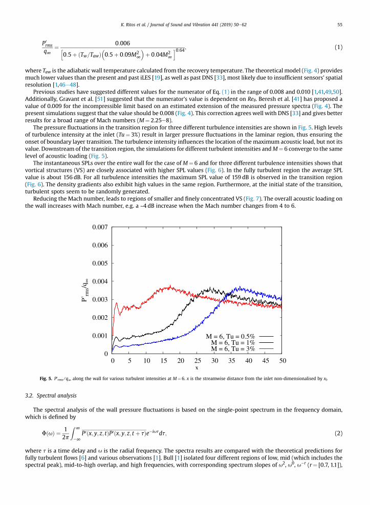
The pressure fluctuations in the transition region for three different turbulence intensities are shown in Fig. 5. High levelsof turbulence intensity at the inlet (Tu¼ 3%) result in larger pressure fluctuations in the laminar region, thus ensuring theonset of boundary layer transition. The turbulence intensity influences the location of the maximum acoustic load, but not itsvalue. Downstream of the transition region, the simulations for different turbulent intensities andM¼ 6 converge to the samelevel of acoustic loading (Fig. 5).

The instantaneous SPLs over the entire wall for the case ofM¼ 6 and for three different turbulence intensities shows thatvortical structures (VS) are closely associated with higher SPL values (Fig. 6). In the fully turbulent region the average SPLvalue is about 156 dB. For all turbulence intensities the maximum SPL value of 159 dB is observed in the transition region(Fig. 6). The density gradients also exhibit high values in the same region. Furthermore, at the initial state of the transition,turbulent spots seem to be randomly generated.

Reducing the Mach number, leads to regions of smaller and finely concentrated VS (Fig. 7). The overall acoustic loading onthe wall increases with Mach number, e.g. a ~4 dB increase when the Mach number changes from 4 to 6.

Fig. 5. P0rms∕q∞ along the wall for various turbulent intensities at M¼ 6. x is the streamwise distance from the inlet non-dimensionalised by xl.

3.2. Spectral analysis

The spectral analysis of the wall pressure fluctuations is based on the single-point spectrum in the frequency domain,which is defined by

FðuÞ ¼ 12p

Z ∞

�∞P0ðx; y; z; tÞP0ðx; y; z; t þ tÞe�iutdt; (2)

where t is a time delay and u is the radial frequency. The spectra results are compared with the theoretical predictions forfully turbulent flows [6] and various observations [1]. Bull [1] isolated four different regions of low, mid (which includes thespectral peak), mid-to-high overlap, and high frequencies, with corresponding spectrum slopes of u2, u0, u�r (r¼ [0.7, 1.1]),

Fig. 6. Instantaneous flow characteristics of the boundary layer at M¼ 6 and three turbulent intensities at the inflow. The density gradient is a side perspective,while the streamwise velocity and SPL are a top-down perspective. The axes in the Tu¼ 0.5% case apply in all other cases too.

K. Ritos et al. / Journal of Sound and Vibration 441 (2019) 50e6256

and u�t (t¼ [7∕3, 5]), respectively (Fig. 8). The low frequency region is influenced by the turbulent motion in the outer part ofthe boundary layer, while high frequencies are influenced by the viscosity and turbulent motion in the inner part of theboundary layer.

According to the theoretical arguments made by Ffowcs-Williams [4] for compressible flows, in the low frequency regionthe scaling should be u / 0. This observation has been confirmed by experimental and numerical studies of supersonic andhypersonic turbulent boundary layers [16,34,41,52]. This is in contrast to the Kraichnan-Phillips theorem for incompressibleflows [1,53,54], which suggests u2.

The mid-to-high overlap frequency region appears at sufficiently high Req values and the spectrum varies as u�r withr¼ 0.7 to 1.1, influenced by the local Reynolds number. This region is associated with pressure-induced eddies in the loga-rithmic region of the boundary layer. Its scaling behaviour was predicted by Bradshaw [5], and was verified theoretically [55]and experimentally [41,51].

Following the u�r region, the spectrum becomes u�7∕3, henceforth called “acoustic-transition”, which was also predictedfor isotropic turbulence by Batchelor [56] and has also been observed in various experiments [48,57,58], as well as verified bynumerical calculations of supersonic turbulent boundary layers [16,52]. At high frequencies the spectrum decaysmore rapidlyreaching a slope proportional to u�5. Sources in the sublayer (yþ< 20) contribute to this frequency region according to thetheoretical prediction of Blake [6], with the scaling being validated experimentally, as well [51,59].

3.3. Fully turbulent region

The spectra at two positions along the plate are presented. The first location corresponds to the end of the transitionregion, which is identified as the point of peak pressure fluctuations and depends on the inlet Mach number. The secondlocation (x¼ 45) is located in the fully turbulent flow. These locations were selected in order to discuss the differences of the

Fig. 7. Instantaneous flow characteristics of the boundary layer for three Mach numbers and Tu¼ 3%. The density gradient is a side perspective, while thestreamwise velocity and SPL are a top-down perspective. The axes in 6 (Tu¼ 0.5% case) apply in all cases here.

K. Ritos et al. / Journal of Sound and Vibration 441 (2019) 50e62 57

transitional and fully turbulent regions. The spectrum roll-off of the fully turbulent flow is shown in Fig. 9. All spectra havebeen filteredwith the ‘smooth bezier’ function of Gnuplot in order to highlight the various scaling regionsmore clearly. Fig. 9bshows both the raw and the filtered PSD. The spectrum roll-off is not affected by filtering. Fig. 9d shows a characteristic non-filtered spectrum where grid convergence is achieved. The low frequency pressure fluctuations are nearly grid-converged.The magnitude of the high-frequency spectrum is under-predicted on the coarsest grid (G1).

Fig. 8. Frequency regions isolated through collective observations by Bull [1].

Fig. 9. PSD in the fully turbulent region. The dashed vertical line in (d) indicated the maximum frequency resolved by mesh G2.

K. Ritos et al. / Journal of Sound and Vibration 441 (2019) 50e6258

The low frequency region yields u / 0, which agrees with the aforementioned analysis. The mid-to-high overlap fre-quency region scales as u�r with the frequency range and slope being Mach number dependent. The value of r lies between1.0 and 1.3 depending on the Mach number. This region also occurs over a broader range of frequencies, as the Mach numberincreases.

The high frequency region of the spectrum, including the “acoustic-transition” scaling (Fig. 8), also appears in the case ofhypersonic turbulent boundary layers. Additionally, the last leg of the high frequency encompasses a region of (approxi-mately) u�8 atM¼ 6 and 8. We attribute this region to high-speed, compressibility effects closer to the wall (yþ< 20). TheMach dependence of the spectrum in fully turbulent boundary layers has also been observed in experiments [60] and nu-merical simulations [16]. Due to the quasi-incompressible nature of the flow near the (iso-thermal) wall, the temperaturefluctuations are significantly reduced.

3.4. End of the transition region

The largest pressure fluctuations occur in the transition region (Figs. 3a and 5) and the spectra results are shown in Fig. 10.Note that for all Mach numbers the transition region contains considerably more low-frequency pressure fluctuationscompared to the fully turbulent boundary layer.

In the low frequency region, the simulations yield u0.3 for all Mach numbers. The rest of the spectrum depends strongly onthe Mach number. For M¼ 4 the mid-frequency region is a plateau, while for M¼ 6 and M¼ 8 the scaling yields u�0.5 andu�0.8, respectively. In the “acoustic-transition” region the scaling yields u�3, u�1.6 and u�2.8 for M¼ 4, M¼ 6 and M¼ 8,respectively. It is clear that the scaling of the spectra at the end of the transition region is different than Batchelor's theoreticalprediction of u�7∕3, which was based on the assumption of isotropic turbulence. The deviation of the scaling behaviour fromu�7∕3 due to the onset of flow anisotropy and localised coherent structures. Near thewall, turbulent flow structures are highlyanisotropic having an ellipsoidal shape [27]. The streamwise turbulent structures are dominant in the mid-buffer layer re-gion; for a supersonic flow (M¼ 2.5) this is around yþz 10 [27].

In the high frequency regime the spectrum scales with u�5, u�6.8 andu�7.8 for the threeMach numbers (Fig.10). Therefore,the high frequency flow regime at the end of the transition region approaches the spectral behaviour of the fully turbulentflow for all Mach numbers. The spectrum's decay is accelerated when increasing the Mach number, namely u�5 forM¼ 4 andu�8 for M¼ 6 and M¼ 8, respectively.

The new spectra scaling applicable to the end of the transition region is summarised in Fig. 11. The low frequency regimescales with k¼ 0.3, while the rest of the spectrum is Mach number dependent. The scaling lies in the intervals r¼ [0.5, 0.8],

Fig. 10. PSD at the end of the transition region.

Fig. 11. Frequency regions in the transition flow region. The scaling factors are: k¼ 0.3, r¼ [0.5, 0.8], t¼ [1.6, 3.0] and s¼ [5, 7.8]. The r scaling does not appear atM¼ 4.

K. Ritos et al. / Journal of Sound and Vibration 441 (2019) 50e62 59

t¼ [1.6, 3.0] and s¼ [5, 7.8] for the mid-to-high frequency overlap, “acoustic-transition” from overlap to high frequency, andhigh-frequency region, respectively.

3.5. Turbulent intensity effects

The turbulent intensity has a small effect on the spectrum at the end of the transition region (Fig. 12a). For Tu¼ 0.5% andTu¼ 1.0% the Reynolds number is slightly higher than Tu¼ 3.0%, thus the spectra for the first two cases are in closeragreement. For Tu¼ 0.5%, the mid-frequency region of u�0.5 appears only within a short range of frequencies.

In the fully turbulent flow, the friction Reynolds number is similar for all turbulent intensities. The turbulent intensityinfluences only the overlap region and the initial part of the high frequency region. The pre-multiplied pressure spectra

Fig. 12. Turbulent intensity effects on the PSD of pressure fluctuations: (a) at the end of transition regionwhere the peak of P0rms magnitude is calculated; (b) fullyturbulent locations with the same Ret. Turbulent intensity effects on the pre-multiplied PSD of the pressure fluctuations. The different x locations correspond tothe end of the transition region.

K. Ritos et al. / Journal of Sound and Vibration 441 (2019) 50e6260

(Fig. 12b) show that the maximum value occurs in the same position irrespective of the turbulent intensity value. However, ahigher turbulent intensity results in a higher amplitude due to the higher energy content of the fluctuation imposed at theinlet.

4. Conclusions

Acoustic effects beneath hypersonic transitional boundary layers have been investigated by performing spatial andspectral analysis of near-wall pressure fluctuations. iLES at different Mach numbers and a range of inlet turbulent intensitieshave been carried out. The simulations have also been validated against DNS and experimental data. The most importantconclusions drawn from the present study are summarised below:

� Laganelli's theoretical model, applicable to the incompressible limit, was modified and validated against iLES, DNS andexperimental data for a range of Mach numbers.

� Increasing the turbulence intensity of the free-stream turbulence influences the location of the maximum acoustic loadbut not its magnitude.

� High SPL values are associated with vortical structures of large streamwise velocity.� Structural panels will be subjected to the strongest acoustic fatigue in the transition region.� Spectral analysis was performed at two points, at the end of the transition and in the fully turbulent flow, and revealed thefollowing:(i) The frequency spectrum is Mach number dependent both for transitional and fully turbulent flows.(ii) The pressure fluctuations in transitional flows are governed by scaling laws that differ from the ones in turbulent

flows. New scaling laws for the wall-pressure fluctuations in the transition region have been presented.(iii) Increasing the free-stream turbulence intensity leads to larger fluctuations in the fully turbulent region.

Future research should aim at the development of improved acoustic models for transitional and fully turbulentcompressible flows, as well as investigation of the effects of acoustic loading on the structural vibration and fatigue ofaerospace structures.

Acknowledgements

This work was sponsored by the Air Force Office of Scientific Research, Air Force Material Command, USAF, under grantnumber FA9550-14-1-0224. The U.S. Government is authorised to reproduce and distribute reprints for Governmentalpurpose notwithstanding any copyright notation thereon. The authors would like to thank S. M. Spottswood and Z. Riley atAFRL Structural Sciences Center, as well as D. Garner (EOARD) for their support. Results were obtained using the EPSRC fundedARCHIE-WeSt High Performance Computer (www.archie-west.ac.uk) under EPSRC grant no. EP/K000586/1.

References

[1] M.K. Bull, Wall-pressure fluctuations beneath turbulent boundary layers: some reflections on forty years of research, J. Sound Vib. 190 (3) (1996)299e315.

[2] S.R. Pate, M.D. Brown, Acoustic Measurements in Supersonic Transitional Boundary Layers, Tech. Rep. AEDC-TR-69-182, ARO Inc, 1969.[3] A.L. Laganelli, A. Martellucci, L.L. Shaw, Wall pressure fluctuations in attached boundary-layer flow, AIAA J. 21 (4) (1983) 495e502.[4] J.E. Ffowcs-Williams, Surface pressure fluctuations induced by boundary layer flow at finite Mach number, J. Fluid Mech. 22 (1965) 507e519.

K. Ritos et al. / Journal of Sound and Vibration 441 (2019) 50e62 61

[5] P. Bradshaw, Inactive motion and pressure fluctuations in turbulent boundary layers, J. Fluid Mech. 30 (2) (1967) 241e258.[6] W.K. Blake, Mechanics of Flow-induced Sound and Vibration, Academic Press, New York, 1986.[7] J.C. Houbolt, On the Estimation of Pressure Fluctuations in Boundary Layers and Wakes, Tech. Rep. TIS 66SD296, General Electric, 1966.[8] L.M. Mack, Boundary Layer Linear Stability Theory, Tech. Rep. 709, AGARD, 1984.[9] J. Sivasubramanian, H.F. Fasel, Direct numerical simulation of transition in a sharp cone boundary layer at mach 6: fundamental breakdown, J. Fluid

Mech. 768 (2015) 175e218.[10] C.-H. Zhang, Q. Tang, C.-B. Lee, Hypersonic boundary-layer transition on a flared cone, Acta Mech. Sin. 29 (1) (2013) 48e53.[11] K.M. Casper, S.J. Beresh, S.P. Schneider, Pressure fluctuations beneath instability wavepackets and turbulent spots in a hypersonic boundary layer, J.

Fluid Mech. 756 (2014) 1058e1091.[12] Y. Zhu, C. Zhang, X. Chen, H. Yuan, J. Wu, S. Chen, C. Lee, Transition in hypersonic boundary layers: role of dilatational waves, AIAA J. 54 (10) (2016)

3039e3049.[13] K.M. Casper, S.J. Beresh, J.F. Henfling, R.W. Spillers, B.O.M. Pruett, Hypersonic wind-tunnel measurements of boundary-layer transition on a slender

cone, AIAA J. 54 (4) (2016) 1250e1263.[14] L. Duan, I. Beekman, M.P. Martín, Direct numerical simulation of hypersonic turbulent boundary layers. Part 3. Effect of Mach number, J. Fluid Mech.

672 (2011) 245e267.[15] K.J. Franko, S.K. Lele, Breakdown mechanisms and heat transfer overshoot in hypersonic zero pressure gradient boundary layers, J. Fluid Mech. 730

(2013) 491e532.[16] L. Duan, M.M. Choudhari, C. Zhang, Pressure fluctuations induced by a hypersonic turbulent boundary layer, J. Fluid Mech. 804 (2016) 578e607.[17] D. Drikakis, Advances in turbulent flow computations using high-resolution methods, Prog. Aero. Sci. 39 (6e7) (2003) 405e424.[18] D. Drikakis, M. Hahn, A. Mosedale, B. Thornber, Large eddy simulation using high resolution and high order methods, Proc. R. Soc. A 367 (2009)

2985e2997.[19] K. Ritos, I.W. Kokkinakis, D. Drikakis, S.M. Spottswood, Implicit large eddy simulation of acoustic loading in supersonic turbulent boundary layers,

Phys. Fluids 29 (4) (2017) 1e11.[20] E.F. Toro, Riemann Solvers and Numerical Methods for Fluid Dynamics, third ed., Springer, 2009.[21] D.S. Balsara, C.W. Shu, Monotonicity preserving weighted essentially non-oscillatory schemes with increasingly high order of accuracy, J. Comput.

Phys. 160 (2) (2000) 405e452.[22] D. Drikakis, W. Rider, High-resolution Methods for Incompressible and Low-speed Flows, Springer, 2005.[23] F. Grinstein, L. Margolin, W. Rider (Eds.), Implicit Large Eddy Simulation: Computing Turbulent Fluid Dynamics, Cambridge University Press, 2007.[24] I.W. Kokkinakis, D. Drikakis, Implicit large eddy simulation of weakly-compressible turbulent channel flow, Comput. Methods Appl. Math. 287 (2015)

229e261.[25] K. Ritos, I.W. Kokkinakis, D. Drikakis, Performance of high-order implicit large eddy simulations, Comput. Fluids 178 (2018) 307e312, https://doi.org/

10.1016/j.compfluid.2018.01.030.[26] K. Ritos, I.W. Kokkinakis, D. Drikakis, Physical insight into a mach 7.2 compression corner flow, in: AIAA Aerospace Sciences Meeting, Kissimmee,

Florida, 2018.[27] K. Ritos, I.W. Kokkinakis, D. Drikakis, Physical insight into the accuracy of finely-resolved iLES in turbulent boundary layers, Comput. Fluids 169 (2018)

309e316.[28] D.K. Wilson, Turbulence Models and the Synthesis of Random Fields for Acoustic Wave Propagation Calculations, Tech. Rep. ARL-TR-1677, Army

Research Laboratory, 1998.[29] J.C.R. Hunt, A.A. Wray, P. Moin, Eddies, Streams, and Convergence Zones in Turbulent Flows, Tech. rep., Center for Turbulence Research, 1988.[30] V. Kol�a�r, J. �Sístek, Corotational and compressibility aspects leading to a modification of the vortex-identification q-criterion, AIAA J. 53 (8) (2015)

2406e2410.[31] L. Brandt, P. Schlatter, D.S. Henningson, Transition in boundary layers subject to free-stream turbulence, J. Fluid Mech. 517 (2004) 167e198.[32] M.P. Martín, Direct numerical simulation of hypersonic turbulent boundary layers. Part 1. initialization and comparison with experiments, J. Fluid

Mech. 570 (2007) 347e364.[33] L. Duan, M.M. Choudhari, Numerical study of pressure fluctuations due to a Mach 6 turbulent boundary layer, in: 51st AIAA Aerospace Sciences

Meeting, 2013, pp. 1e16.[34] C. Zhang, L. Duan, M.M. Choudhari, Effect of wall cooling on boundary-layer-induced pressure fluctuations at Mach 6, J. Fluid Mech. 822 (2017) 5e30.[35] M. El�ena, J.P. Lacharme, Experimental study of a supersonic turbulent boundary layer using a laser Doppler anemometer, J. Mec. Theor. Appl. 7 (2)

(1988) 90e175.[36] P. Bradshaw, Compressible turbulent shear layers, Annu. Rev. Fluid Mech. 9 (1977) 33e54.[37] P.D. Welch, The use of Fast Fourier Transform for the estimation of power spectra: a method based on time averaging over short, modified perio-

dograms, IEEE Trans. Audio Electroacoust. AU-15 (1967) 70e73.[38] A. Martellucci, L. Chaump, D. Rogers, D. Smith, Experimental determination of the aeroacoustic environment about a slender cone, AIAA J. 11 (5) (1973)

635e642.[39] B.J. Moskal, Investigation of the Sonic Fatigue Characteristics of Randomly Excited Aluminum, Tech. Rep. CR-425, NASA, 1966.[40] J. Soovere, The effect of acoustic/thermal environments on advanced composite fuselage panels, J. Aircraft 22 (4) (1985) 257e263.[41] S.J. Beresh, J.F. Henfling, R.W. Spillers, B.O.M. Pruett, Fluctuating wall pressures measured beneath a supersonic turbulent boundary layer, Phys. Fluids

23 (075110) (2011) 1e16.[42] R.D. Shattuck, Sound Pressures and Correlations of Noise on the Fuselage of a Jet Aircraft in Flight, Tech. Rep. TN-D-1086, NASA, 1961.[43] W.W. Willmarth, C.E. Wooldridge, Measurements of the fluctuating pressure at the wall beneath a thick turbulent boundary layer, J. Fluid Mech. 14 (2)

(1962) 187e210.[44] W.W. Willmarth, F.W. Roos, Resolution and structure of the wall pressure field beneath a turbulent boundary layer, J. Fluid Mech. 22 (1) (1965) 81e94.[45] M.K. Bull, Wall-pressure fluctuations associated with subsonic turbulent boundary layer flow, J. Fluid Mech. 28 (4) (1967) 719e754.[46] W.W. Willmarth, Pressure fluctuations beneath turbulent boundary layers, Annu. Rev. Fluid Mech. 7 (1975) 13e36.[47] M.K. Bull, A.S.W. Thomas, High frequency wall-pressure fluctuations in turbulent boundary layers, Phys. Fluids 19 (4) (1976) 597e599.[48] G. Schewe, On the structure and resolution of wall-pressure fluctuations associated with turbulent boundary layer flow, J. Fluid Mech. 134 (1983)

311e328.[49] R.M. Lueptow, Transducer resolution and the turbulent wall pressure spectrum, J. Acoust. Soc. Am. 97 (1) (1995) 370e378.[50] M.C. Goody, R.L. Simpson, Surface pressure fluctuations beneath two¼ and three-dimensional turbulent boundary layers, AIAA J. 38 (10) (2000)

1822e1831.[51] S.P. Gravante, A.M. Naguip, C.E. Wark, H.M. Nagib, Characterization of the pressure fluctuations under a fully developed turbulent boundary layer, AIAA

J. 36 (10) (1998) 1808e1816.[52] M. Bernardini, S. Pirozzoli, Wall pressure fluctuations beneath supersonic turbulent boundary layers, Phys. Fluids 23 (085102) (2011) 1e11.[53] R.H. Kraichnan, Pressure fluctuations in turbulent flow over a flat plate, J. Acoust. Soc. Am. 28 (3) (1956) 378e390.[54] O.M. Phillips, On the aerodynamic surface sound from a plane turbulent boundary, Proc. R. Soc. A 234 (1198) (1956) 327e335.[55] R.L. Panton, J.H. Linebarger, Wall pressure spectra calculations for equilibrium boundary layers, J. Fluid Mech. 65 (2) (1974) 261e287.[56] G.K. Batchelor, Pressure fluctuations in isotropic turbulence, Proc. Camb. Phil. Soc. 47 (1951) 359e374.[57] Y. Tsuji, T. Ishihara, Similarity scaling of pressure fluctuation in turbulence, Phys. Rev. E 68 (2003), 026309.

K. Ritos et al. / Journal of Sound and Vibration 441 (2019) 50e6262

[58] R. Camussi, M. felli, F. Pereira, G. Aloisio, A.D. Marco, Statistical properties of wall pressure fluctuations over a forward-facing step, Phys. Fluids 20(2008), 075113.

[59] T.M. Farabee, M.J. Casarella, Spectral features of wall pressure fluctuations beneath turbulent boundary layers, Phys. Fluids A 3 (10) (1991) 2410e2420.[60] J. Laufer, Some statistical properties of the pressure field radiated by a turbulent boundary layer, Phys. Fluids 7 (8) (1964) 1191e1197.