Journal of Theoretical Biology 266 (2010) 504–515

Contents lists available at ScienceDirect

Journal of Theoretical Biology

0022-51

doi:10.1

� Corr

E-m

ddhoff@

journal homepage: www.elsevier.com/locate/yjtbi

Natural selection and veridical perceptions

Justin T. Mark �, Brian B. Marion, Donald D. Hoffman

Department of Cognitive Science, University of California, Irvine, CA 92697, USA

a r t i c l e i n f o

Article history:

Received 2 April 2010

Received in revised form

23 June 2010

Accepted 21 July 2010Available online 24 July 2010

Keywords:

Evolution

Replicator dynamics

Interface games

Sensation

Game theory

93/$ - see front matter & 2010 Elsevier Ltd. A

016/j.jtbi.2010.07.020

esponding author. Tel.: +1 720 234 7985.

ail addresses: jtmark@uci.edu (J.T. Mark), bm

uci.edu (D.D. Hoffman).

a b s t r a c t

Does natural selection favor veridical perceptions, those that more accurately depict the objective

environment? Students of perception often claim that it does. But this claim, though influential, has not

been adequately tested. Here we formalize the claim and a few alternatives. To test them, we introduce

‘‘interface games,’’ a class of evolutionary games in which perceptual strategies compete. We explore, in

closed-form solutions and Monte Carlo simulations, some simpler games that assume frequency-

dependent selection and complete mixing in infinite populations. We find that veridical perceptions can

be driven to extinction by non-veridical strategies that are tuned to utility rather than objective reality.

This suggests that natural selection need not favor veridical perceptions, and that the effects of selection

on sensory perception deserve further study.

& 2010 Elsevier Ltd. All rights reserved.

1. Introduction

Students of perception often claim that perception, in general,estimates the truth. They argue that creatures whose perceptionsare more true are also, thereby, more fit. Therefore, due to naturalselection, the accuracy of perception grows over generations, sothat today our perceptions, in most cases, approximate the truth.

They admit that there are, on occasion, illusory percepts; butthese appear, most often, in psychology labs with contriveddisplays. And they acknowledge limits to perception; visible light,for instance, occupies a small portion of the electromagneticspectrum, and visible objects inhabit a modest range of spatialscales. But they maintain that, for middle-sized objects to whichvision is adapted, the colors, shapes and motions that we see are,most often, good estimates of the true values in the real world.

Their statements on this are clear. Lehar (2003), for instance,argues that ‘‘The primary function of perception [is] that ofgenerating a fully spatial virtual-reality replica of the externalworld in an internal representation.’’ Geisler and Diehl (2003) say,‘‘In general, (perceptual) estimates that are nearer the truth havegreater utility than those that are wide of the mark.’’ Palmer(1999), in his textbook Vision Science, asserts that, ‘‘evolutionarilyspeaking, visual perception is useful only if it is reasonablyaccurate.’’ Yuille and Bulthoff (1996) concur, saying, ‘‘visualperception yinvolves the evolution of an organism’s visual

ll rights reserved.

arion@uci.edu (B.B. Marion),

system to match the structure of the world and the codingscheme provided by nature.’’

If perception estimates the truth then, they argue, a naturalmodel of perception is Bayesian estimation. In such a model forvisual perception, the eye receives some images, I, and the brainthen estimates the true values of scene properties, S, such asshape and color (see, e.g., Knill and Richards, 1996). To do so, itcomputes the conditional probability measure PðSjIÞ, and thenselects a value for which this conditional probability is, say,maximized.

By Bayes’ rule, PðSjIÞ ¼ PðIjSÞPðSÞ=PðIÞ. The term P(S) denotes the‘‘prior’’ distribution of true values of physical properties, such asshapes and colors. The ‘‘likelihood’’ term PðIjSÞ describes how thephysical world maps to images at the eye. P(I) normalizes allvalues to probabilities. These terms, as used in the computationsof the brain, are shaped by selection, so that its estimates areaccurate. As a result, the priors and likelihoods used by the brainaccurately reflect the true priors and likelihoods in the world.

This account of perception and its evolution is, no doubt,appealing. But it depends crucially on the claim that truerperception is fitter perception. This raises two questions. Doesevolutionary theory support this claim? And what, precisely, ismeant by true perception?

We answer the second question, in the next section, byformalizing possible relations between perception and reality.Then, to answer the first question, we use evolutionary games toexplore the relative fitness of these possible relations. We findthat truth can fare poorly if information is not free; costs for timeand energy required to gather information can impair the fitnessof truth. What often fares better is a relation between perceptionand reality akin to the relation between a graphical user interface

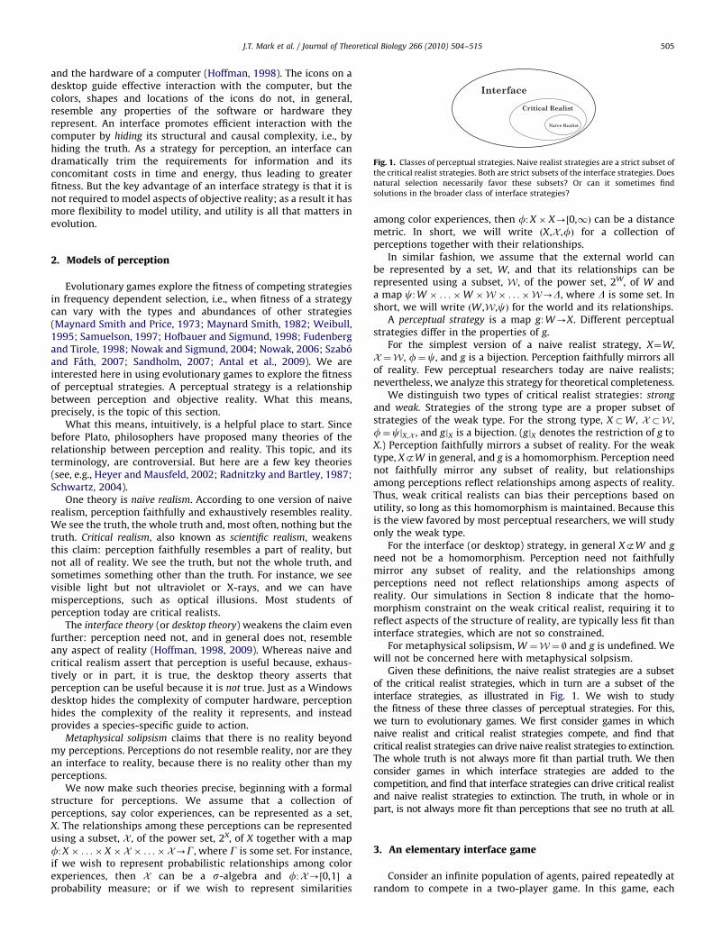
Fig. 1. Classes of perceptual strategies. Naive realist strategies are a strict subset of

the critical realist strategies. Both are strict subsets of the interface strategies. Does

natural selection necessarily favor these subsets? Or can it sometimes find

solutions in the broader class of interface strategies?

J.T. Mark et al. / Journal of Theoretical Biology 266 (2010) 504–515 505

and the hardware of a computer (Hoffman, 1998). The icons on adesktop guide effective interaction with the computer, but thecolors, shapes and locations of the icons do not, in general,resemble any properties of the software or hardware theyrepresent. An interface promotes efficient interaction with thecomputer by hiding its structural and causal complexity, i.e., byhiding the truth. As a strategy for perception, an interface candramatically trim the requirements for information and itsconcomitant costs in time and energy, thus leading to greaterfitness. But the key advantage of an interface strategy is that it isnot required to model aspects of objective reality; as a result it hasmore flexibility to model utility, and utility is all that matters inevolution.

2. Models of perception

Evolutionary games explore the fitness of competing strategiesin frequency dependent selection, i.e., when fitness of a strategycan vary with the types and abundances of other strategies(Maynard Smith and Price, 1973; Maynard Smith, 1982; Weibull,1995; Samuelson, 1997; Hofbauer and Sigmund, 1998; Fudenbergand Tirole, 1998; Nowak and Sigmund, 2004; Nowak, 2006; Szaboand Fath, 2007; Sandholm, 2007; Antal et al., 2009). We areinterested here in using evolutionary games to explore the fitnessof perceptual strategies. A perceptual strategy is a relationshipbetween perception and objective reality. What this means,precisely, is the topic of this section.

What this means, intuitively, is a helpful place to start. Sincebefore Plato, philosophers have proposed many theories of therelationship between perception and reality. This topic, and itsterminology, are controversial. But here are a few key theories(see, e.g., Heyer and Mausfeld, 2002; Radnitzky and Bartley, 1987;Schwartz, 2004).

One theory is naive realism. According to one version of naiverealism, perception faithfully and exhaustively resembles reality.We see the truth, the whole truth and, most often, nothing but thetruth. Critical realism, also known as scientific realism, weakensthis claim: perception faithfully resembles a part of reality, butnot all of reality. We see the truth, but not the whole truth, andsometimes something other than the truth. For instance, we seevisible light but not ultraviolet or X-rays, and we can havemisperceptions, such as optical illusions. Most students ofperception today are critical realists.

The interface theory (or desktop theory) weakens the claim evenfurther: perception need not, and in general does not, resembleany aspect of reality (Hoffman, 1998, 2009). Whereas naive andcritical realism assert that perception is useful because, exhaus-tively or in part, it is true, the desktop theory asserts thatperception can be useful because it is not true. Just as a Windowsdesktop hides the complexity of computer hardware, perceptionhides the complexity of the reality it represents, and insteadprovides a species-specific guide to action.

Metaphysical solipsism claims that there is no reality beyondmy perceptions. Perceptions do not resemble reality, nor are theyan interface to reality, because there is no reality other than myperceptions.

We now make such theories precise, beginning with a formalstructure for perceptions. We assume that a collection ofperceptions, say color experiences, can be represented as a set,X. The relationships among these perceptions can be representedusing a subset, X , of the power set, 2X, of X together with a mapf:X � . . .� X � X � . . .� X-G, where G is some set. For instance,if we wish to represent probabilistic relationships among colorexperiences, then X can be a s-algebra and f:X-½0,1� aprobability measure; or if we wish to represent similarities

among color experiences, then f:X � X-½0,1Þ can be a distancemetric. In short, we will write ðX,X ,fÞ for a collection ofperceptions together with their relationships.

In similar fashion, we assume that the external world canbe represented by a set, W, and that its relationships can berepresented using a subset, W, of the power set, 2W, of W anda map c:W � . . .�W �W � . . .�W-D, where D is some set. Inshort, we will write ðW ,W,cÞ for the world and its relationships.

A perceptual strategy is a map g:W-X. Different perceptualstrategies differ in the properties of g.

For the simplest version of a naive realist strategy, X¼W,X ¼W, f¼c, and g is a bijection. Perception faithfully mirrors allof reality. Few perceptual researchers today are naive realists;nevertheless, we analyze this strategy for theoretical completeness.

We distinguish two types of critical realist strategies: strong

and weak. Strategies of the strong type are a proper subset ofstrategies of the weak type. For the strong type, X �W , X �W,f¼cjX,X , and gjX is a bijection. (gjX denotes the restriction of g toX.) Perception faithfully mirrors a subset of reality. For the weaktype, XgW in general, and g is a homomorphism. Perception neednot faithfully mirror any subset of reality, but relationshipsamong perceptions reflect relationships among aspects of reality.Thus, weak critical realists can bias their perceptions based onutility, so long as this homomorphism is maintained. Because thisis the view favored by most perceptual researchers, we will studyonly the weak type.

For the interface (or desktop) strategy, in general XgW and g

need not be a homomorphism. Perception need not faithfullymirror any subset of reality, and the relationships amongperceptions need not reflect relationships among aspects ofreality. Our simulations in Section 8 indicate that the homo-morphism constraint on the weak critical realist, requiring it toreflect aspects of the structure of reality, are typically less fit thaninterface strategies, which are not so constrained.

For metaphysical solipsism, W ¼W ¼ | and g is undefined. Wewill not be concerned here with metaphysical solpsism.

Given these definitions, the naive realist strategies are a subsetof the critical realist strategies, which in turn are a subset of theinterface strategies, as illustrated in Fig. 1. We wish to studythe fitness of these three classes of perceptual strategies. For this,we turn to evolutionary games. We first consider games in whichnaive realist and critical realist strategies compete, and find thatcritical realist strategies can drive naive realist strategies to extinction.The whole truth is not always more fit than partial truth. We thenconsider games in which interface strategies are added to thecompetition, and find that interface strategies can drive critical realistand naive realist strategies to extinction. The truth, in whole or inpart, is not always more fit than perceptions that see no truth at all.

3. An elementary interface game

Consider an infinite population of agents, paired repeatedly atrandom to compete in a two-player game. In this game, each

J.T. Mark et al. / Journal of Theoretical Biology 266 (2010) 504–515506

agent must choose one of three territories. Each territory containstwo resources (e.g., food and water) which may, or may not, becorrelated. The quantity of each resource ranges from 1 to 100,and their sum is the utility of that territory. (Later we considerutility that is a nonmonotonic function of quantity.)

When an agent chooses a territory, the utility of that territorybecomes the agent’s fitness. The agent that chooses second mustselect between the remaining two territories. Each agent uses oneof two perceptual strategies in its attempt to find the territorywith greatest utility.

The simple strategy, which is a critical realist strategy, observesonly one resource per territory, say food. If the quantity of thatresource is above a threshold, it sees ‘‘green,’’ otherwise its sees‘‘red.’’ If there is only one green territory, the agent chooses thatterritory. If there is more than one green territory, the agentchooses among them at random. If there are only red territories, itagain chooses at random.

The truth strategy, which is a naive realist strategy, sees theexact quantity of each resource in each territory, and chooses thebest available territory.

Seeing more data takes more time. So, in the simplest versionof this game, simple chooses first when competing againsttruth. For more complex versions, priority of choice is settledprobabilistically.

Similarly, seeing more data takes more energy, so truth

requires more energy than simple. We subtract the cost of energyfrom the utility that each agent gets from its territory.

There are, of course, infinite variations on this simple game.The number of resources and their correlations can be varied. Thenumber of territories can be increased. The simple agent might seethree or more colors rather than just two. We explore some ofthese variations below, using Monte Carlo simulations. But first,to fix ideas, we start with a particularly simple variation that wecan solve in closed form. We find that the costs in time and energycharged to truth can exceed the benefits it receives from perfectknowledge, so that truth ends up less fit than simple. We derivethe payoffs to truth and simple with mathematical detail, in orderto make the structure of interface games quite clear.

Truth 47

63

22

71

94

11

SimpleFood = 47

Water = 63

Food = 22

Water = 71

Food = 94

Water = 11

Food > 50Otherwise

Fig. 2. Illustration of the truth and simple perceptual strategies. In the middle are

three territories, each having a food value and water value between 1 and 100. The

perceptions of truth are shown to the left of each territory. Since truth sees the

exact values, its perceptions are identical to the food and water values of each

territory. The perceptions of simple are shown to the right of each territory. Here

simple sees the color green if the food value of a territory is 450; otherwise it sees

red. (For interpretation of the references to color in this figure legend, the reader is

referred to the web version of this article.)

4. A single resource game

In this game, the external world has three territories, T1, T2, T3,and one resource, say food, that takes discrete values in the setV ¼ {1,2,y,m}. The possible values of food in the three territoriesform our external world space W ¼ V1 � V2 � V3, where each Vi isa copy of V. We assume that W has a measurable structureW ¼ 2W , where 2W is the power set of W; each set AAW is anevent. Food is uniformly, and independently, distributed on eachmeasurable space ðVi,V iÞ, i ¼ 1, 2, 3, where V i ¼ 2Vi .

We consider two perceptual strategies: truth and simple. Theperceptual space of truth is the measurable space ðY ,YÞ ¼ ðW ,WÞ.The perceptual space of simple is the measurable space ðX,XÞ,where X ¼ C1 � C2 � C3, for Ci¼{0,1} and X ¼ 2X . We think of 0 asthe percept ‘‘red’’ and 1 as ‘‘green;’’ for mnemonic convenience,we sometimes write R instead of 0 and G instead of 1. Whensimple views a territory, it does not see the actual food value ofthat territory; instead it sees either red or green. It sees green ifthe actual food value exceeds some boundary bAV , and redotherwise. This is, of course, a particularly simplistic form ofperceptual categorization, adopted here for its mathematicalsimplicity; this evolutionary game can be modified to use morecomplex forms of perceptual categorization.

The sensory map from the world to the perceptual space oftruth is the identity map, g:W-Y . In the case of simple, for anyboundary bAV , we define a map fb:V

3-X, induced by the map

f Vb :V-C given by

f Vb ðvÞ ¼

0 if 1rvrb,

1 if bovrm,

(ð1Þ

for any vAV . The map f Vb assigns a color to a single territory V, and

fb uses f Vb to assign a color to each of the three territories. This is

illustrated in Fig. 2.Observe that the perceptual space of the simple strategy, as

defined above, can be written as

X ¼ f000,001, . . . ,111g, ð2Þ

or, in our R and G notation

X ¼ fRRR,RRG, . . . ,GGGg, ð3Þ

where, for instance, RRG means the first two territories are redand the other is green.

4.1. Simple

To use evolutionary game theory to analyze the competitionbetween the simple and truth strategies, we must first computethe expected payoffs to each strategy when competing with itselfand with the other strategy. These payoffs contribute to theevolutionary fitness of each strategy.

We now compute expected food payoffs for simple. If simple isfirst to choose a territory, then there are two events of interest:G0 ¼ {0 green territories} ¼ {RRR}, and its complement G123 ¼ {1,2, or 3 green territories}¼X�G0. If G0 occurs, then simple mustpick a red territory; otherwise simple picks a green territory, sinceit always picks green if possible. The probabilities for these eventsare

PðG0Þ ¼bm

� �3

,

PðG123Þ ¼ 1�PðG0Þ, ð4Þ

where b=m is the probability of a single red territory, and we usethe fact that the territories are independently distributed.

The expected payoff of a green territory is

EðvjGÞ ¼mþbþ1

2, ð5Þ

J.T. Mark et al. / Journal of Theoretical Biology 266 (2010) 504–515 507

because food is distributed uniformly on ½bþ1,m� and so has anexpectation midway between bþ1 and m. The expected payoff ofa red territory is

EðvjRÞ ¼bþ1

2, ð6Þ

because food is distributed uniformly on ½1,b� in red territories.Multiplying these payoffs by their probabilities, we find theexpected payoff to simple when choosing first:

Eð1ÞS ðvjb,mÞ ¼ PðG0Þbþ1

2þPðG123Þ

mþbþ1

2: ð7Þ

where the subscript S denotes the simple strategy and thesuperscript (1) indicates choosing first. Taking the derivative of(7) with respect to the boundary, b, we find that simple maximizesits expected payout if it has the boundary b¼m=

ffiffiffi3p

.In this game, simple chooses first when competing against

truth, so its expected payoff against truth is

ESjT ¼ Eð1ÞS ðvjb,mÞ, ð8Þ

where SjT denotes simple competing against truth.We now compute the expected payoff for simple vs simple. One

simple agent is randomly picked to choose first. We have justcomputed the expected payoffs for simple choosing first, so wenow consider the payoffs for simple choosing second. In this case,the events of interest are G01 ¼ {0 or 1 green territories} and G23

¼ {2 or 3 green territories}. For the event G01, simple must choosered (since there is at most one green territory, and the first agenttook it) and for G23 simple chooses green. The probabilityassociated with each event is then

PðG01Þ ¼bm

� �3

þ3bm

� �2 m�bm

� �, ð9aÞ

PðG23Þ ¼ 1�PðG01Þ, ð9bÞ

where in (9a), the first term is the probability that all threeterritories are red, and the second term is the probability ofexactly 1 green territory.

Using the expected payoffs for red and green territories from(5) and (6), we compute the expected payoff for simple choosingsecond to be

Eð2ÞS ðvjb,mÞ ¼ PðG01Þbþ1

2þPðG23Þ

mþbþ1

2: ð10Þ

Using (7) and (10) we can now define the expected payoff tosimple when competing against another simple agent to be

ESjS ¼12½Eð1ÞS ðvjb,mÞþEð2ÞS ðvjb,mÞ�, ð11Þ

which is simply the average of Eqs. (7) and (10).

4.2. Truth

In this simplified game, when truth and simple compete, simple

chooses first but might not choose the best territory. Theprobability that it chooses the best depends on the number ofgreen territories. For instance, if there is just one green territory,then simple will choose it and get the best. Truth then chooses thebest of the remaining territories. Thus, the key events forcalculating the expected payoffs for truth when competing againstsimple are G0 ¼ {RRR}, G1 ¼ {RRG,RGR,GRR}, G2 ¼ {GGR,GRG,RGG},and G3 ¼ {GGG} with probabilities

PðG0Þ ¼bm

� �3

,

PðG1Þ ¼ 3bm

� �2 m�bm

� �,

PðG2Þ ¼ 3bm

� �m�b

m

� �2

,

PðG3Þ ¼m�b

m

� �3

: ð12Þ

The payoff for each event can be found using (1) ‘‘orderstatistics’’ and (2) the probability that simple chooses the bestterritory. The rth order statistic of a statistical sample is itsr th-smallest value. For instance, if one samples, with replace-ment, three numbers from a uniform distribution on the integersbetween 1 and 100, the first order statistic is the smallest of thesethree numbers.

In particular, for our purposes here, order statistics allow us tocalculate the maximum value of a sample (see, e.g., Calik andGungor, 2004). This value depends only on the number of red andgreen territories, because red and green territories have differentuniform distributions. Red territories draw from the set ½1,b�,whereas green territories draw from ½bþ1,m�. Thus, let j be thenumber of red territories (0r jr3) and k the number of greenterritories (0rkr3), so that j+k is the total number of territories(three in the example at hand). Then the cumulative distributionfunction (cdf) of the rth order statistic for V is either

Fr:jðvjRÞ ¼

Xj

i ¼ r

j

i

� �v

b

� �i

1�v

b

� �j�i

if 1rvrb,

1 if bovrm,

8>><>>: ð13aÞ

Fr:kðvjGÞ ¼

0 if 1rvrb,Xk

i ¼ r

k

i

� �v�bm�b

� �i

1�v�bm�b

� �k�i

if bovrm:

8>><>>: ð13bÞ

Eq. (13a) describes the cdf of the rth order statistic for redterritories. In particular, Fj:j is the cdf of the maximum valuedrawn from j red territories. Eq. (13b) does the same for greenterritories. Eqs. (13a) and (13b) can be used to calculate theexpected value of the rth order statistic for red and greenterritories (Calik and Gungor, 2004):

Er:jðvjRÞ ¼Xm

v ¼ 0

½1�Fr:nðvjRÞ�, ð14aÞ

Er:kðvjGÞ ¼Xm

v ¼ 0

½1�Fr:nðvjGÞ�: ð14bÞ

Ej:jðvjRÞ is the expected value of the best of j red territories;similarly Ek:kðvjGÞ is the expected value of the best of k greenterritories. Using (14a) and (14b) we can compute the expectedvalue of the best territory chosen by truth for any combination of j

red and k green territories. For this computation, the mostrelevant events are again G0, G1, G2, and G3 because they allow usto compute the probability that simple chooses the best territoryin each event. The expected payoffs for truth associated with eachevent are

EðvjG0Þ ¼23 E3:3ðvjRÞþ

13E2:3ðvjRÞ, ð15aÞ

EðvjG1Þ ¼ E2:2ðvjRÞ, ð15bÞ

EðvjG2Þ ¼12 E2:2ðvjGÞþ

12E1:2ðvjGÞ, ð15cÞ

EðvjG3Þ ¼23 E3:3ðvjGÞþ

13E2:3ðvjGÞ: ð15dÞ

Appendix A gives formulas for each Ei:j in these equations.Eq. (15a) describes the event G0 consisting of 0 green (i.e., threered territories). In this case simple chooses randomly from amongthe three territories. There is a 2/3 chance that simple will not

Table 2Selection dynamics.

Simple wins a4c and b4d

Truth wins aoc and bod

Bistable a4c and bod

Stably coexist aoc and b4d

Neutral a ¼ c and b ¼ d

Fig. 3. Stable evolutionary outcomes of the single resource game.

J.T. Mark et al. / Journal of Theoretical Biology 266 (2010) 504–515508

choose the best territory, in which case truth will choose the bestterritory. This gives us the first term in (15a). There is a 1/3 chancethat simple will choose the best territory, in which case truth willchoose the second best territory. This gives us the second term in(15a). Eq. (15b) describes the event G1 consisting of one green andtwo red territories. In this case simple chooses the green, i.e., thebest, territory, forcing truth to choose the best of two redterritories. Eq. (15c) describes the event G2 consisting of twogreen and one red territories. Simple chooses randomly betweenthe two green territories. Half of the time simple will choose thebest territory forcing truth to take the second best territory.Otherwise, simple will choose the second best territory allowingtruth to choose the best and giving the second term in (15c). For(15d), describing the event G3, there are three green territoriesand simple, once again, chooses randomly among them. Thus truth

will take the best territory 2/3 of the time, and the second best 1/3of the time.

Using the probabilities for the events G0 through G3 from (12),and their expected payoffs from (15), the expected payoff for truth

when competing against simple is

ETjSðvjb,mÞ ¼X3

i ¼ 0

EðvjGiÞPðGiÞ: ð16Þ

When truth competes against truth, each chooses the bestterritory available. Thus, to find the expected payoff we need onlycompute the expected values of the best and second bestterritories, viz., E3:3(v) and E2:3(v). The expected payoff to truth

when competing against truth is then

ETjT ðvÞ ¼12½E3:3ðvÞþE2:3ðvÞ�, ð17Þ

where

E3:3ðvÞ ¼3m2þ2m�1

4m, ð18aÞ

E2:3ðvÞ ¼mþ1

2ð18bÞ

(see Calik and Gungor, 2004, Section 6).

5. Evolutionary dynamics

Given the expected payoffs from the previous section, evolu-tionary game theory can be used to study the long terminteractions between simple and truth. For instance, when doesone strategy drive the other to extinction, and when do the twostably coexist? To this end, we create a payoff matrix describingthe competition between the strategies, as presented in Table 1.

The payoff matrix is defined as follows. Simple gets payoff a

when competing against simple and payoff b when competingagainst truth. Truth gets payoff c when competing against simple

and payoff d when competing against truth. The payoff to astrategy is taken to be the fitness of that strategy, i.e., itsreproductive success. The fitness of a strategy in one generationdetermines the proportion of players using that strategy in thenext generation. Asymptotically, i.e., after many generations,there are five possible outcomes for the two strategies, presentedin Table 2, that are determined by the payoffs in Table 1.

Table 1Payoff matrix.

Simple Truth

Simple a b

Truth c d

A strategy ‘‘wins’’ if, asymptotically, it drives the other strategyto extinction regardless of the initial proportions of the strategies;a winning strategy is the best response to itself and the otherstrategy. Two strategies stably coexist if, independent of theirinitial proportions, those proportions approach asymptoticallystable values; each strategy is the best reply to the other strategy,but not to itself. Two strategies are bistable if their initialproportions determine which strategy drives the other toextinction; each strategy is the best response to itself, but notto the other strategy. Two strategies are neutral if their initialproportions, whatever they happen to be, are preserved asymp-totically.

The payoffs in Table 1 for simple and truth are the expectedvalues calculated previously (Eqs. (8), (11), (16), and (17)) minusthe cost of information. This cost is computed by multiplying thecost per bit of information, ce, by the number of bits used. We thinkof ce as the energy expenditure that each strategy uses to acquireand process information, and to choose a territory. This is central tothe analysis of perceptual strategies, since processing moreinformation takes, on average, more time and energy. Accountingfor information costs, the entries for the payoff matrix are

a¼ ESjS�3ce,

b¼ ESjT�3ce,

c¼ ETjS�3celog2ðmÞ,

d¼ ETjT�3celog2ðmÞ: ð19Þ

Simple sees 1 bit of information per territory, since it only sees redor green. Therefore, because there are three territories, it sees atotal of 3 bits of information. Truth sees log2ðmÞ bits of informationper territory, which for m¼100 is approximately 20 bits. There arealso, of course, energy costs for decision, not just for perception.But for simplicity of analysis we ignore these here.

We now plot, in Fig. 3, how ce and the red/green boundary usedby simple affect the asymptotic performance of each strategy.White is where simple wins, black where truth wins, and graywhere the two strategies stably coexist.

As seen from Fig. 3, simple drives truth to extinction for mostboundaries. Even if simple has a poor boundary (e.g., 0–10 or90–100), truth wins only for small ce. This suggests that as the costof information increases, simpler perceptual strategies canenhance survival.

J.T. Mark et al. / Journal of Theoretical Biology 266 (2010) 504–515 509

6. Environmental complexity

The evolutionary game we have studied so far is quite simple.Now, to better understand the strengths and weaknesses of eachstrategy, we increase the complexity of the external world in threeways: we vary the number of territories, the number of resourcesper territory, and the correlations between resources. One mightexpect that additional complexity would favor truth but, as weshow in this section, simple can still drive truth to extinction.

0 0.2 0.4 0.6 0.8 10

0.05

0.1

0.15

0.2

Correlation

Cos

t per

Bit

Fig. 5. Effect of correlation on the maximum cost per bit at which truth drives to

extinction an optimal simple agent in an environment with seven territories and

four resources. When r¼ 0 this maximum cost corresponds to about 11.6% of the

expected payout to truth, and when r¼ 1 it corresponds to about 1%.

6.1. Correlated resources

We first modify our simple game by adding a single resource(e.g., water) to each territory, and then study the effects of varyingthe correlation between food and water. Since truth sees everyaspect of the world, each additional resource will increase thenumber of bits it sees and the energy it expends. Simple only seesfood and therefore expends no energy on perceiving water. If thecorrelation between food and water is high and simple happens topick a territory with a large food value, then it probably also gets ahigh water value; simple effectively gains information about waterwithout expending more energy. However, it gains little ifcorrelations are low. In nature, of course, both high and lowcorrelations are found between various resources.

As before, the quantities of food and water have uniformdistributions on [1,2,y,m]; we now assume they have correlationr. We studied the effect of correlation on the evolutionary stablestrategies by running Monte Carlo simulations of the competitionbetween truth and simple. Each input to the payoff matrix wascomputed as the average of 106 interactions, which was sufficientto provide stable values.

Fig. 4 shows that as correlation increases, truth does steadilyworse when simple has a central boundary, but does better whensimple has a boundary at either extreme. The range of boundaries forwhich simple drives truth to extinction also increases with increasedcorrelation. The increased correlation effectively gives simple freeaccess to more information, allowing it to compete more effectively.

Fig. 4. Evolutionarily stable strategies with increasing correlation. When r¼ 0, truth ca

which corresponds to an energy cost of about 6.8% of the expected payout to truth.

It is useful now to define the optimal boundary for simple to bethe boundary that maximizes its expected payoff against truth,i.e., that maximizes b in the payoff matrix of Table 1. Fig. 5 showsthat, as the correlation between resources increases, a simple

agent using an optimal boundary does better against truth. In thisfigure, we quantify the performance of truth by the maximum costper bit of information at which truth drives the optimal simple

agent to extinction. This figure assumes seven territories and fourresources per territory which, we shall see, is favorable for truth;the effects of adding more territories and resources are discussedin more detail in the next section.

6.2. Additional resources

We now increase the complexity of the game by adding moreresources to each territory. Fig. 6 shows that adding resourcesimproves the fitness of truth up to a point, but then adding moreresources beyond this slowly reduces the fitness of truth. Thefitness of truth increases initially because, with each additionalresource, simple sees a smaller proportion of the information in

n survive against an optimal simple agent so long as the cost per bit is about o0:2,

Exp

ecte

d M

axim

um V

alue

100

90

80

70

60

502

Number of Territories

4 6 8 10 12 14

J.T. Mark et al. / Journal of Theoretical Biology 266 (2010) 504–515510

the environment and, as a result, is less likely to choose the bestterritory. This allows truth to pick the best territory more often.

As we continue to add resources, though, the territoriesbecome more homogenous, i.e., the difference between the bestand worst territories becomes smaller. Therefore, while truth ismore likely to choose a better territory than simple, the differencein their payouts becomes less significant. At the same time, truth’scost increases with each additional resource while simple’s costremains constant. This combination of higher costs and moresimilar territories leads to the asymptotic decrease in truth’sfitness and, in consequence, an asymptotic increase in the fitnessof simple.

Fig. 8. Expected maximum value for n territories.

6.3. Additional territories

We now return to one resource per territory and increase thenumber of territories. The additional territories provide a slightlymore complex environment in which we compare the twostrategies. Both simple and truth are charged as before for eachadditional bit of information they use to see the extra territoriesin the environment. But while both strategies see increases incosts, truth’s cost increases significantly faster with the increasesin information.

Fig. 7 shows that while the initial addition of territories aidstruth, the costs of seeing more than eight territories overcomesthe benefits. To understand this effect, we revisit how theexpected maximum value of n territories changes withincreasing n. Recall from Eq. (18a) that the expected maximumvalue for three territories is approximately 75. If we add anadditional territory, that value jumps to about 80. As we continueto add more territories; however, the increases in the expected

5 10 15 20 25 300

0.02

0.04

0.06

0.08

0.1

0.12

Number of Resources

Cos

t per

Bit

Fig. 6. Effect of the number of resources on the maximum cost per bit at which

truth drives to extinction an optimal simple agent. In an environment with

10 resources per territory, this maximum cost corresponds to about 3.7% of the

expected payout to truth, and for 30 resources it is about 3.0%.

5 10 15 20 25 300

0.05

0.1

0.15

0.2

Number of Territories

Cos

t per

Bit

Fig. 7. Effect of the number of territories on the maximum cost per bit at which

truth drives to extinction an optimal simple agent. In an environment with eight

territories, this maximum cost corresponds to about 10% of the expected payout to

truth, and for 30 territories it is about 18.8%.

maximum territory level off as shown in Fig. 8. For truth, thismeans that for more than eight territories, the increase in costrequired to see the extra territories exceeds the increase in itsexpected maximum payout. However, for the optimal simple, theincrease in cost required to see each extra territory (i.e., one bit)does not exceed the increase in its expected maximum payout.This payout grows quickly for simple because, for any fixedboundary o100, as the number of territories increases thenumber of green territories will also increase. Therefore theoptimal simple uses a higher boundary and receives a greaterpayout. As a result, we see that simple maintains its evolutionarilyadvantage as complexity increases.

7. Optimality in a complex environment

The previous section focused on the effects of increasingenvironmental complexity in the competition between truth andthe optimal simple agent. The simulations show that, even in morecomplex environments, the optimal simple agent still drives truth

to extinction for small cost-per-bit values. We now study how theoptimal boundary for the simple agent changes with increasingenvironmental complexity. We also study strategies that usemultiple, optimally placed boundaries, rather than the singleboundary used by simple.

7.1. Optimal boundary placement

As we increase complexity by adding more territories, theboundary for the optimal simple agent shifts. With moreterritories available, the probability increases that one of themhas a large food value. To increase the probability that it willchoose a more valuable territory, the optimal simple agent musthave a higher boundary, so that only territories with high foodvalues are labeled green. In other words, it is useful for simple tobecome more discriminating in its selection of territories, asshown in Fig. 9.

7.2. Multiple category strategies

We now study how a simple agent performs if, instead of twocategories, it has n categories; we will call this an nCat agent. Forexample, a 3Cat agent might have boundaries at 70 and 40 andwould label territories 470 ‘‘green,’’ territories 440 but r70‘‘yellow,’’ and territories r40 ‘‘red.’’ The three perceptualcategories are ordered, e.g., green4yellow4red. In addition tothis perceptual order, the agent has another order describing itsdecision strategy, such as yellow4green4red, i.e., choose yellowterritories if available, then green,then red. The nCat agent is ahybrid of simple and truth (e.g., at 100 categories the nCat agent isidentical to truth). This allows us to study how additional

5 10 15 20 25 3055

60

65

70

75

80

85

90

Opt

imal

Bou

ndar

y

Number of Territories

Fig. 9. Increase in the optimal boundary as environmental complexity increases.

0 10 20 30 40 50 60 70 80 90 100

0 10 20 30 40 50 60 70 80 90 100

Fig. 10. Optimal boundary placement in a simple game (3-territories, 2-resources,

and no correlation). Each strategy has a preference order that is identical to its

perceptual order (e.g., green4yellow4red). (For interpretation of the references to

color in this figure legend, the reader is referred to the web version of this article.)

0 10 20 30 40 50 60 70 80 90 100100

105

110

115

120

125

Number of Boundaries

Ave

rage

Pay

off

Cost per bit = 0Cost per bit = 0.1Cost per bit = 0.25Cost per bit = 0.5Cost per bit = 0.75Cost per bit = 1

Fig. 11. Effect of additional boundaries on the expected payout of the nCat agent

with evenly spaced boundaries. Environment consists of three territories each

with two uncorrelated resources and an expected payout of approximately 125 for

the best territory.

122

123

124

125

126

Pay

off

J.T. Mark et al. / Journal of Theoretical Biology 266 (2010) 504–515 511

perceptual information about the environment affects the evolu-tionary fitness of a strategy.

Fig. 10 shows the optimal placement for one through fiveboundaries in a game with three territories and two uncorrelatedresources.

As the number of categories increases, the optimal nCat agentreceives more information about the environment. If the nCat

agent wished to glean the most information about its environ-ment, it would space its n�1 boundaries evenly because thedistribution of resources in this environment is uniform. Instead,the lower part of the scale gets relatively few boundaries whilethe higher end becomes crowded with additional boundaries. Thismirrors results from Komarova and Jameson (2008) showing thatoptimal boundary placement is governed to a large degree byutility. The optimal nCat agent, in this case, has more boundariesnear the high end of the resource scale, allowing it to betterdistinguish among those territories with high utility. In thismanner, the nCat agent maximizes its fitness.

0 10 20 30 40 50 60 70 80 90 100117

118

119

120

121

Number of Boundaries

Ave

rage Cost per bit = 0

Cost per bit = 0.1

Cost per bit = 0.25

Cost per bit = 0.5

Cost per bit = 0.75

Cost per bit = 1

Fig. 12. Effect of additional categories on the expected payout of the nCat agent

with evenly spaced boundaries when cost increases logarithmically with the

number of bits. Environment consists of three territories each with two

uncorrelated resources and an expected payout of approximately 125 for the best

territory.

7.3. Truth seeking strategies

As we saw in the previous section, the optimal nCat agent hascategories with unevenly spaced boundaries, allowing it to be intune with the utility of its environment. However, since theresources in the environment have uniform distributions, if thenCat had categories with evenly spaced boundaries, this wouldallow it to be better in tune with the truth of its environment (forinstance, in the sense of a least squares estimate of the true valueof a resource). The categories best tuned to utility need not be thecategories best tuned to truth.

In this section, we study the categories best tuned to truth, i.e.,we study the nCat agent with evenly spaced boundaries. As thenumber of boundaries increases, this agent sees a more refinedrepresentation of the truth of its environment, and will approximatethe truth strategy as the number of boundaries approaches 100.

Fig. 11 shows the expected payoff for the nCat agent as thenumber of evenly spaced boundaries increase. For the ‘‘cost perbit¼0’’ curve, there is no increase in payoff for additionalboundaries beyond 10 boundaries.

Fig. 11 also shows that if the cost of information is greater than0, then there is an optimal number of categories that maximizesthe expected payoff. As the cost of information increases, thisoptimal number of categories decreases. Adding further cate-gories actually decreases the expected payoff and, in consequence,will probably decrease fitness.

One might object that Fig. 11 assumes that the cost ofinformation grows linearly with the number of bits, thus ignoringthe possibility that there could be an economy of scale. Toinvestigate this objection we ran new simulations, shown inFig. 12, in which the cost for information only growslogarithmically with the number of bits. Again we see that thereis no increase in payoff for additional categories beyond about 16categories.

Util

ity

0 20 30 40 50 60 80 90 100

100

Util

ity

0 20 30 40 50 60 80 90 100

CR3 (Critical Realist)

IF3 (Interface)

0

100

0

Resource Quantity

Resource Quantity

10 70

10 70

Fig. 13. (A) Optimal boundary placement on a Gaussian utility structure for a 3Cat

critical realist. (B) A 3Cat interface strategy for a Gaussian utility structure. Because

the perceptual map of an interface strategy is not required to be a homomorphism

of the structure of reality, it can instead be tuned to the utilities that are critical to

evolutionary fitness.

J.T. Mark et al. / Journal of Theoretical Biology 266 (2010) 504–515512

8. Interface strategies

One might argue that the simulations discussed so far suggest thatperceptions need not resemble reality to be fit. After all, the simple

strategy sees only red or green, and not the reality of its simulatedenvironment, viz., food and other resources with values ranging from1 to 100. Moreover, red and green are arbitrary representations andcould just as easily be replaced by blue and yellow, smoothand rough, pen and pencil, or even nonsense syllables such asdax and vox; none of these resemble food, water, or 1–100 in anyway. And yet, in many simulations, simple drives truth to extinction.

However, one could counter that simple’s perceptions stillpreserve a vestige of truth. Even though green and red do notresemble the truth, if simple orders its perceptual categoriesgreen 4 red then this reflects a true feature of the environment:every food value that leads to a green perception is greater thanevery food value that leads to a red perception. (It also happens, inthis special case, that green reflects greater utility than red; but ingeneral the order on perceptual categories need not be the sameas the utility order.) This homomorphism between the order inthe environment and the order on perceptual categories is whywe, in Section 3, call simple a critical-realist strategy. Thus, onecould argue that the simulations so far show only that somecritical-realist strategies, which see limited but true informationabout the environment, can be fit.

This raises the question of the fitness of interface strategies: Ifwe eliminate the last vestige of truth in the perceptions of anagent, i.e., if we eliminate any homomorphism between environ-ment and perceptions, can a perceptual strategy still be fit? Herewe show that the answer is yes. Interface strategies canoutcompete critical realist strategies, and can continue to do sowhen naive realist strategies are also present. But first, we brieflydiscuss nonlinear utilities.

8.1. Gaussian utilities

Our simulations, so far, posit a specific linear relationshipbetween utility and quantity of resources, in which, e.g., 10 unitsof food yield twice the payout of 5. Of course utilities in natureneed not fit this model. For a thirsty mouse, a little dew mighthave more utility than a large lake. For a hungry shark, a smalltuna might have more utility than a large whale. The utility ofeating spices depends on local annual temperature (Billing andSherman, 1998) and the utility of geophagy, the deliberate eatingof dirt, depends on the phenolic content of local plants(Krishnamani and Mahaney, 2000).

The spice and geophagy examples illustrate that utilities ofresources can interact with each other and with other aspects ofthe environment. The mouse and shark examples illustrate that,even if such interactions are ignored, utilities can vary nonlinearlywith the quantity of resources. For now, we will omit interactionsbetween utilities, and simply introduce a truncated Gaussianutility function independently on each resource in the environ-ment. In this case, agents receive the highest payout by choosingterritories with resources falling inside an optimal midrange,rather than by finding the greatest quantity of resources.

This poses a new problem, because perceptual informationabout resource quantities is not enough to determine the payoutof each territory. In order to pick the best territory, a strategymust know the payout associated with each possible resourcequantity. We must now charge each strategy for both seeing thequantity and knowing the utility of each resource, and its costbecomes

ce½trlog2ðqÞ�þck½rqnb�, ð20Þ

where ce is again the cost per bit of information, ck is the cost perbit of knowledge about utility values, t is the number ofterritories, r is number of resources, q is the number of perceptualcategories for that strategy, and nb is the number of bits used torepresent the utility of a resource quantity. In the case of truth, wetake q to be 100.

In this situation, the optimal simple agent has its boundary justbelow the peak of the Gaussian curve, so that its green categorycontains this maximum value.

An optimal critical realist with three perceptual categories(red, yellow, green) and perceptual order red o yellow o greenis illustrated in Fig. 13(A); we will call it CR 3. Its decision rulewould be to prefer yellow to green, and green to red. Notice thatthe order governing its decision rule is red o green o yellowwhich differs from its perceptual order. Even though perceptualorders and decision rules can differ, together they coevolve.

An interface strategy is illustrated in Fig. 13(B). It has fourboundaries, but only three perceptual categories (red, yellow,green), so we call it IF 3. As is clear in the figure, the resourcevalues that get mapped to the perceptual category yellow are notall contiguous, nor the resource values that get mapped to red.Thus, this mapping is not a homomorphism. However, it is bettertuned to what really matters in evolution, namely utility. Thiskind of mapping is not possible for the critical realist because itsperceptions must be homomorphic to relationships in reality. Thisrestriction limits the flexibility of the critical realist to be tuned toutilities.

8.2. Three strategy games

We now have the framework to directly compare the threeperceptual strategies described at the start of this paper. Takingtruth to be a naive realist strategy, CR 3 to be a critical realiststrategy, and IF 3 to be an interface strategy, then, by includingall three strategies in one population, we can evaluate the fitnessof each strategy relative to the others by simulating theirevolutionary dynamics through successive generations.

J.T. Mark et al. / Journal of Theoretical Biology 266 (2010) 504–515 513

In our games involving three strategies, the agents arerepeatedly paired at random to compete. This gives a 3�3 payoffmatrix and, unlike in two-player games, we cannot immediatelycalculate which strategy survives and which goes extinct. Insteadwe compute the time derivatives of the frequencies of eachstrategy using the replicator equation (Hofbauer and Sigmund,1998; Nowak, 2006; Taylor and Jonker, 1978),

_X i ¼ Xi½fið~X Þ�fð~X Þ�, ð21Þ

where fð~X Þ is the average fitness and, for each strategy i, Xi

denotes its frequency, _X i its time derivative and fið~X Þ its fitness.

Here, fið~X Þ ¼

Pnj ¼ 1 Pijxj where Pij is the payoff matrix, and

fð~X Þ ¼P

ifið~X Þxi.

We plot the resulting dynamics as a flow field on a 2-simplex(see Fig. 14), where each vertex i represents a populationcomposed entirely of strategy i, each point on the edge oppositeto vertex i represents a population devoid of strategy i, and eachinterior point represents a population containing all threestrategies.

In Fig. 14, the vertices represent the naive-realist (truth),critical-realist (CR 3), and interface strategies (IF 3), competing inan environment with a Gaussian utility structure.

We assume that the truth agent assigns a utility to each of the100 possible resource values, so that nb in (20) is log2ð100Þ; sinceCR 3 and IF 3 only need to order their three categories, their nb in

25

50

75

25

25

50

75

CR3

Truth

IF3

25

50

7525

50

75

CR3

Truth

IF3

Cost = 1%

Cost = 10%

50 75

25 50 75

Fig. 14. Competition between truth, CR 3, and IF 3 in a game with three territories

and one resource per territory. Utility is given by a Gaussian with mean 50 and

standard deviation 20. Arrows indicate evolutionary flows. In (A) the cost to truth

is 1% of its expected payout averaged over competitions with all three strategies

(cost per bit ¼ 0.0074). In (B) the cost to truth is 10% (cost per bit ¼ 0.074). Payoff

matrices for these competitions can be found in Appendix B.

(20) is log2ð3Þ. We also assume that ck¼ce/10, making energycosts of perception and knowledge of utility roughly on a par.Instead of varying over the cost per bit, ce, as we have done inprevious figures, we compute the cost to truth as a percentage oftruth’s expected payout averaged over competitions with all threestrategies. The cost to CR 3 and IF 3 is then computed from (20)and truth’s cost. In this way, the cost for each strategy can bedirectly compared to the expected payoff for truth.

As shown in Fig. 14, for low costs truth dominates and forhigher costs IF 3 dominates; in fact, IF 3 dominates for costs44:25%, truth dominates for costs o4:29%, and in between theycoexist. For these competitions, CR 3 is driven to extinction solong as the initial population contains IF 3 agents. In populationswith no IF 3 agents, CR 3 dominates truth for costs 49:3%, isdominated by truth for costs o9:9%, and in between they coexist.

In order to show that IF 3 does not drive truth and CR 3 toextinction only in this isolated case, we ran simulations withadditional territories and resources. We first increased thenumber of territories. In an environment with 30 territories andone resource per territory, IF 3 drives CR 3 and truth to extinctionfor costs 42:8% of truth’s expected payoff.

We then increased the number of resources. In an environmentwith three territories and 30 resources per territory, IF 3 and CR 3each have three categories per resource but use nb ¼ log2ð100Þ, sothat they can adequately represent the expected utility of eachcategory. In this case IF 3 drives CR 3 and truth to extinction forcosts 40:5% of truth’s expected payoff. These simulations showthat, due to the large costs required for truth to see more complexenvironments, IF 3 is in fact more fit than truth in theseenvironments with increased complexity.

In summary, these competitions between naive realist, criticalrealist and interface strategies show that natural selection doesnot always favor naive realism or critical realism, and that inmany scenarios only the interface strategy survives.

9. Discussion

Perceptual researchers typically assume that ‘‘it is clearlydesirable (say, from an evolutionary point of view) for anorganism to achieve veridical percepts of the world’’ (Feldman,2009, p. 875). They assume, that is, that truer perceptions areipso facto more fit. Although they acknowledge that naturalselection can shape perception to be a ‘‘bag of tricks’’ or heuristics(Ramachandran, 1990), they assume that these tricks or heuristicsare short cuts to the truth.

We tested this assumption using standard tools of evolu-tionary game theory. We found that truer perceptions need not bemore fit: Natural selection can send perfectly, or partially, trueperceptions to extinction when they compete with perceptionsthat use niche-specific interfaces which hide the truth in order tobetter represent utility. Fitness and access to truth are logicallydistinct properties. More truthful perceptions do not entailgreater fitness.

One key insight here is that perceptual information is not free.For every bit of information gleaned by perception there aretypically costs in time and energy. These costs can of course bedefrayed. To reduce costs in time, for instance, neurons canprocess information in parallel. But each additional neuron in aparallel architecture requires additional energy. Costs in time andenergy can trade off, but not be eliminated.

A second key insight is that perceptual information is shapedby natural selection to reflect utility, not to depict reality. Utilitydepends idiosyncratically on the biological needs of eachparticular organism. Idiosyncracies in utility will necessarily leadto concomitant differences in perception, even for organisms that

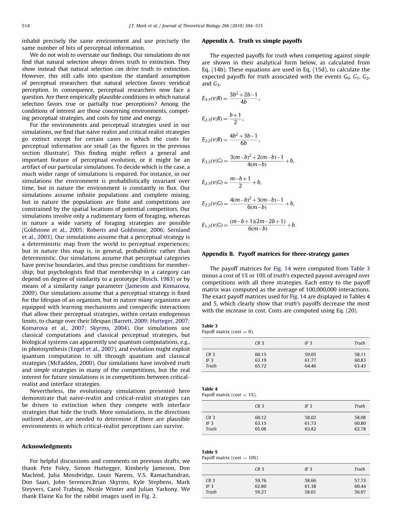
Table 3Payoff matrix (cost ¼ 0).

CR 3 IF 3 Truth

CR 3 60.15 59.05 58.11

IF 3 63.19 61.77 60.83

Truth 65.72 64.46 63.43

Table 4Payoff matrix (cost ¼ 1%).

CR 3 IF 3 Truth

CR 3 60.12 58.02 58.08

IF 3 63.15 61.73 60.80

Truth 65.08 63.82 62.78

J.T. Mark et al. / Journal of Theoretical Biology 266 (2010) 504–515514

inhabit precisely the same environment and use precisely thesame number of bits of perceptual information.

We do not wish to overstate our findings. Our simulations do not

find that natural selection always drives truth to extinction. Theyshow instead that natural selection can drive truth to extinction.However, this still calls into question the standard assumptionof perceptual researchers that natural selection favors veridicalperception. In consequence, perceptual researchers now face aquestion. Are there empirically plausible conditions in which naturalselection favors true or partially true perceptions? Among theconditions of interest are those concerning environments, compet-ing perceptual strategies, and costs for time and energy.

For the environments and perceptual strategies used in oursimulations, we find that naive realist and critical realist strategiesgo extinct except for certain cases in which the costs forperceptual information are small (as the figures in the previoussection illustrate). This finding might reflect a general andimportant feature of perceptual evolution, or it might be anartifact of our particular simulations. To decide which is the case, amuch wider range of simulations is required. For instance, in oursimulations the environment is probabilistically invariant overtime, but in nature the environment is constantly in flux. Oursimulations assume infinite populations and complete mixing,but in nature the populations are finite and competitions areconstrained by the spatial locations of potential competitors. Oursimulations involve only a rudimentary form of foraging, whereasin nature a wide variety of foraging strategies are possible(Goldstone et al., 2005; Roberts and Goldstone, 2006; Sernlandet al., 2003). Our simulations assume that a perceptual strategy isa deterministic map from the world to perceptual experiences;but in nature this map is, in general, probabilistic rather thandeterministic. Our simulations assume that perceptual categorieshave precise boundaries, and thus precise conditions for member-ship; but psychologists find that membership in a category candepend on degree of similarity to a prototype (Rosch, 1983) or bymeans of a similarity range parameter (Jameson and Komarova,2009). Our simulations assume that a perceptual strategy is fixedfor the lifespan of an organism, but in nature many organisms areequipped with learning mechanisms and conspecific interactionsthat allow their perceptual strategies, within certain endogenouslimits, to change over their lifespan (Barrett, 2009; Hutteger, 2007;Komarova et al., 2007; Skyrms, 2004). Our simulations useclassical computations and classical perceptual strategies, butbiological systems can apparently use quantum computations, e.g.,in photosynthesis (Engel et al., 2007), and evolution might exploitquantum computation to sift through quantum and classicalstrategies (McFadden, 2000). Our simulations have involved truth

and simple strategies in many of the competitions, but the realinterest for future simulations is in competitions between critical-realist and interface strategies.

Nevertheless, the evolutionary simulations presented heredemonstrate that naive-realist and critical-realist strategies canbe driven to extinction when they compete with interfacestrategies that hide the truth. More simulations, in the directionsoutlined above, are needed to determine if there are plausibleenvironments in which critical-realist perceptions can survive.

Table 5Payoff matrix (cost ¼ 10%)

CR 3 IF 3 Truth

CR 3 59.76 58.66 57.73

IF 3 62.80 61.38 60.44

Truth 59.27 58.01 56.97

Acknowledgments

For helpful discussions and comments on previous drafts, wethank Pete Foley, Simon Huttegger, Kimberly Jameson, DonMacleod, Julia Mossbridge, Louis Narens, V.S. Ramachandran,Don Saari, John Serences,Brian Skyrms, Kyle Stephens, MarkSteyvers, Carol Trabing, Nicole Winter and Julian Yarkony. Wethank Elaine Ku for the rabbit images used in Fig. 2.

Appendix A. Truth vs simple payoffs

The expected payoffs for truth when competing against simple

are shown in their analytical form below, as calculated fromEq. (14b). These equations are used in Eq. (15d), to calculate theexpected payoffs for truth associated with the events G0, G1, G2,and G3.

E3:3ðvjRÞ ¼3b2þ2b�1

4b,

E2:3ðvjRÞ ¼bþ1

2,

E2:2ðvjRÞ ¼4b2þ3b�1

6b,

E3:3ðvjGÞ ¼3ðm�bÞ2þ2ðm�bÞ�1

4ðm�bÞþb,

E2:3ðvjGÞ ¼m�bþ1

2þb,

E2:2ðvjGÞ ¼4ðm�bÞ2þ3ðm�bÞ�1

6ðm�bÞþb,

E1:2ðvjGÞ ¼ðm�bþ1Þð2m�2bþ1Þ

6ðm�bÞþb:

Appendix B. Payoff matrices for three-strategy games

The payoff matrices for Fig. 14 were computed from Table 3minus a cost of 1% or 10% of truth’s expected payout averaged overcompetitions with all three strategies. Each entry to the payoffmatrix was computed as the average of 100,000,000 interactions.The exact payoff matrices used for Fig. 14 are displayed in Tables 4and 5, which clearly show that truth’s payoffs decrease the mostwith the increase in cost. Costs are computed using Eq. (20).

J.T. Mark et al. / Journal of Theoretical Biology 266 (2010) 504–515 515

References

Antal, T., Nowak, M., Traulsen, A., 2009. Strategy abundance in 2�2 games forarbitrary mutation rates. Journal of Theoretical Biology 257, 340–344.

Barrett, J.A., 2009. The evolution of coding in signaling games. Theory and Decision67, 223–237.

Billing, J., Sherman, P.W., 1998. Antimicrobial functions of spices: why some like ithot. The Quarterly Review of Biology 73, 3–49.

Calik, S., Gungor, M., 2004. On the expected values of sample maximum of orderstatistics from a discrete uniform distribution. Applied Mathematics Compu-tation 157, 695–700.

Engel, G.S., Tessa, R.C., Read, E.L., Ahn, T., Mancal, T., Cheng, Y., Blankenship, R.E.,Fleming, G.R., 2007. Evidence for wavelike energy transfer through quantumcoherence in photosynthetic systems. Nature 446, 782–786.

Feldman, J., 2009. Bayes and the simplicity principle in perception. PsychologicalReview 116, 875–887.

Fudenberg, D., Tirole, J., 1998. Game Theory, sixth ed MIT Press, Cambridge, MA.Geisler, W.S., Diehl, R.L., 2003. A Bayesian approach to the evolution of perceptual

and cognitive systems. Cognitive Science 27, 379–402.Goldstone, R.L., Ashpole, B.C., Roberts, M.E., 2005. Knowledge of resources and

competitors in human foraging. Psychonomic Bulletin & Review 12, 81–87.Heyer, D., Mausfeld, R. (Eds.), 2002. Perception and the Physical World:

Psychological and Philosophical Issues in Perception. Wiley, New York.Hofbauer, J., Sigmund, K., 1998. Evolutionary Games and Population Dynamics.

Cambridge University Press, Cambridge.Hoffman, D.D., 1998. Visual Intelligence: How We Create What We See.

W.W. Norton, New York.Hoffman, D.D., 2009. The interface theory of perception. In: Dickinson, S., Tarr, M.,

Leonardis, A., Schiele, B. (Eds.), Object Categorization: Computer and HumanVision Perspectives. Cambridge University Press, Cambridge.

Hutteger, S.M., 2007. Evolution and the explanation of meaning. Philosophy ofScience 74, 1–27.

Jameson, K.A., Komarova, N.L., 2009. Evolutionary models of color categorization.Journal of the Optical Society of America A 26 (6), 1414–1436.

Knill, D., Richards, W. (Eds.), 1996. Perception as Bayesian Inference. CambridgeUniversity Press, Cambridge.

Komarova, N.L., Jameson, K.A., Narens, L., 2007. Evolutionary models of colorcategorization based on discrimination. Journal of Mathematical Psychology51, 359–382.

Komarova, N.L., Jameson, K.A., 2008. Population heterogeneity and color stimulusheterogeneity in agent-based color categorization. Journal of TheoreticalBiology 253, 680–700.

Krishnamani, R., Mahaney, W., 2000. Geophagy among primates: adaptivesignificance and ecological consequences. Animal Behavior 59, 899–915.

Lehar, S., 2003. Gestalt isomorphism and the primacy of subjective consciousexperience: a Gestalt Bubble model. Behavioral and Brain Sciences 26, 375–444.

Maynard Smith, J., 1982. Evolution and the Theory of Games. CambridgeUniversity Press, Cambridge.

Maynard Smith, J., Price, G.R., 1973. The logic of animal conflict. Nature 246, 15–18.McFadden, J., 2000. Quantum Evolution. W.W. Norton, New York.Nowak, M.A., 2006. Evolutionary Dynamics: Exploring the Equations of Life.

Belknap Harvard University Press, Cambridge, MA.Nowak, M.A., Sigmund, K., 2004. Evolutionary dynamics of biological games.

Science 303, 793–799.Palmer, S.E., 1999. Vision Science: Photons to Phenomenology. MIT Press,

Cambridge, MA.Radnitzky, G., Bartley, W.W. (Eds.), 1987. Evolutionary Epistemology, Theory of

Rationality, and the Sociology of Knowledge. Open Court, La Salle, Illinois.Ramachandran, V.S., 1990. Interactions between motion, depth, color and form:

the utilitarian theory of perception. In: Blakemore, C. (Ed.), Vision: Coding andEfficiency. Cambridge University Press, Cambridge.

Roberts, M.E., Goldstone, R.L., 2006. EPICURE: Spatial and knowledge limitations ingroup foraging. Adaptive Behavior 14, 291–313.

Rosch, E., 1983. Prototype classification and logical classification: the two systems.In: Scholnick, E.K. (Ed.), New Trends in Conceptual Representation: Challengesto Piagets Theory?. Lawrence Erlbaum Associates Hillsdale.

Samuelson, L., 1997. Evolutionary Games and Equilibrium Selection. MIT Press,Cambridge, MA.

Sandholm, W.H., 2007. Population Games and Evolutionary Dynamics. MIT Press,Cambridge, MA.

Schwartz, R., 2004. Perception. Blackwell Publishing, Malden, MA.Sernland, E., Olsson, O., Holmgren, N.M.A., 2003. Does information sharing

promote group foraging? Proceedings of the Royal Society of London 2701137–1141.

Skyrms, B., 2004. The Stag Hunt and the Evolution of Social Structure. CambridgeUniversity Press, Cambridge.

Szabo, G., Fath, G., 2007. Evolutionary games on graphs. Physics Reports 446,97–216.

Taylor, P., Jonker, L., 1978. Evolutionary stable strategies and game dynamics.Mathematical Bioscience 40, 145–156.

Weibull, J., 1995. Evolutionary Game Theory. MIT Press, Cambridge, MA.Yuille, A., Bulthoff, H., 1996. Bayesian decision theory and psychophysics. In: Knill,

D., Richards, W. (Eds.), Perception as Bayesian Inference. CambridgeUniversity Press, Cambridge.