journal of theoretical politics - duke universitypeople.duke.edu/~gsv5/jtp2014.pdf · journal of...

http://jtp.sagepub.com/Journal of Theoretical Politics

http://jtp.sagepub.com/content/26/3/355The online version of this article can be found at:

DOI: 10.1177/0951629813502709

2014 26: 355 originally published online 15 November 2013Journal of Theoretical PoliticsJustin Fox and Georg Vanberg

Narrow versus broad judicial decisions

Published by:

http://www.sagepublications.com

can be found at:Journal of Theoretical PoliticsAdditional services and information for

http://jtp.sagepub.com/cgi/alertsEmail Alerts:

http://jtp.sagepub.com/subscriptionsSubscriptions:

http://www.sagepub.com/journalsReprints.navReprints:

http://www.sagepub.com/journalsPermissions.navPermissions:

What is This?

- Nov 15, 2013OnlineFirst Version of Record

- Nov 28, 2013OnlineFirst Version of Record

- Jun 19, 2014Version of Record >>

at DUKE UNIV on September 3, 2014jtp.sagepub.comDownloaded from at DUKE UNIV on September 3, 2014jtp.sagepub.comDownloaded from

http://jtp.sagepub.com/

http://jtp.sagepub.com/content/26/3/355

http://www.sagepublications.com

http://jtp.sagepub.com/cgi/alerts

http://jtp.sagepub.com/subscriptions

http://www.sagepub.com/journalsReprints.nav

http://www.sagepub.com/journalsPermissions.nav

http://jtp.sagepub.com/content/26/3/355.full.pdf

http://jtp.sagepub.com/content/early/2013/11/27/0951629813502709.full.pdf

http://jtp.sagepub.com/content/early/2013/11/13/0951629813502709.full.pdf

http://online.sagepub.com/site/sphelp/vorhelp.xhtml



Article

Narrow versus broad judicialdecisions

Journal of Theoretical Politics2014, Vol. 26(3) 355–383

©The Author(s) 2013Reprints and permissions:

sagepub.co.uk/journalsPermissions.navDOI:10.1177/0951629813502709

jtp.sagepub.com

Justin FoxDepartment of Political Science, Washington University in St. Louis, USA

Georg VanbergDepartment of Political Science, Duke University, USA

AbstractA central debate among judges and legal scholars concerns the appropriate scope of judicialopinions: should decisions be narrow, and stick to the facts at hand, or should they be broad,and provide guidance in related contexts? A central argument for judicial ‘minimalism’ holds thatjudges should rule narrowly because they lack the knowledge required to make general rules togovern unknown future circumstances. In this paper, we challenge this argument. Our argumentfocuses on the fact that, by shaping the legal landscape, judicial decisions affect the policies thatare adopted, and that may therefore subsequently be challenged before the court. Using a simplemodel, we demonstrate that in such a dynamic setting, in which current decisions shape futurecases, judges with limited knowledge confront incentives to rule broadly precisely because theyare ignorant.

KeywordsJudicial review; judicial minimalism; constitutional interpretation; broad and narrow rulings

1. IntroductionThe US Supreme Court exercises judicial review in the course of resolving particulardisputes.1 It is not surprising that the contextual nature of decisions has given rise tocompeting views regarding their appropriate scope. One position, exemplified by JusticeAntonin Scalia, holds that opinions should not be tied too closely to the facts of theparticular cases that give rise to them. Instead, the justices ought to develop broad rulesthat enhance predictability in the law and provide clear guidance to policymakers, lower

Corresponding author:Georg Vanberg, Department of Political Science, Duke University, Durham, NC 27708, USA.Email: [email protected]

at DUKE UNIV on September 3, 2014jtp.sagepub.comDownloaded from


356 Journal of Theoretical Politics 26(3)

courts, and individuals in related circumstances (see e.g. Scalia, 1989). Others, includingformer Justice Sandra Day O’Connor and Chief Justice John Roberts, have argued for theopposite approach. In this view, judicial opinions should be narrow, that is, they should‘stick to the case at hand’ and avoid, to the extent possible, rules that wander beyond thespecific issues presented. As Chief Justice Roberts put it in a commencement addressat Georgetown University Law School in 2006: ‘If it’s not necessary to decide more todispose of a case, in my view, it’s necessary not to decide more (Associate Press, 2006).’

The difference between these approaches is best illustrated with the help of exam-ples. Consider Employment Division v. Smith, a 1990 case involving a challenge to thedenial of unemployment benefits by individuals who had lost jobs as a result of con-suming peyote, a controlled substance, during a native American religious ceremony.The Supreme Court rejected the claim that the employees’ right to the free exercise ofreligion had been infringed. In doing so, Justice Scalia’s opinion crafted a broad rule.Rather than restrict itself to upholding the denial of unemployment benefits as a result ofdrug use, the opinion established that governments are generally free to impose restric-tions that affect religious practice without violating the First Amendment if there existsa legitimate (non-religious) reason for regulating the behavior. As a result, the opinionprovides relatively clear guidance to lower courts, governments, and citizens with respectto the constitutionality of a wide range of potential restrictions on religious behavior.2 Incontrast, in City of Ontario v. Quon, a 2010 decision, the Supreme Court held that theaudit of a police officer’s city-issued pager did not constitute a violation of the FourthAmendment. The Court’s decision was narrow, focusing on the fact that, in this instance,administrators had a valid, work-related reason for the audit. Justice Kennedy’s opinionexplicitly rejected the notion of devising a more general rule to govern searches of theelectronic communications of government employees.

One prominent argument in favor of such judicial ‘minimalism’ focuses on the factthat judges may lack the knowledge required to develop broad rules that are appropriatefor (unknown) future circumstances. As a result, broad opinions run the risk of announ-cing rules that turn out to be inappropriate ex post, and that may be difficult or costlyto change. To avoid such ‘lock-in’, judges ought to rule narrowly, and only extend rules‘piece-meal’ as new cases allow them to do so. As Cass Sunstein has put it, a court‘does best if it proceeds narrowly and if it avoids steps that might be confounded byunanticipated circumstances’ (Sunstein, 2005, p. 1903). To do so is no more than anacknowledgment ‘that there is much that it does not know’ (Sunstein, 1999, p. ix). Indeed,Justice Kennedy’s opinion in Quon stresses this ‘knowledge problem’ as a rationale forits limited scope:

Prudence counsels caution before the facts in the instant case are used to establish far-reachingpremises . . . A broad holding concerning employees’ privacy expectations vis-à-vis employer-provided technological equipment might have implications for future cases that cannot bepredicted. It is preferable to dispose of this case on narrower grounds.

In this paper, we consider this ‘epistemological’ argument for judicial minimalism.Specifically, we ask whether judges with limited knowledge may, under certain circum-stances, have reason to issue broad decisions precisely because they know that there is‘much that they don’t know’. Perhaps surprisingly, our answer to this question is ‘yes’.



Fox and Vanberg 357

What is the intuition behind this claim? Some of the most significant decisions thatjudges make are those that evaluate the constitutionality of policies adopted by legisla-tors and bureaucrats. When a court, especially a high court, issues such a decision, itprovides guidance about what is (or is not) constitutionally acceptable in the court’s eyes.Policymakers react, and adjust policy in light of the court’s ruling. Abortion policy inthe US states, for example, has been shaped by the Supreme Court’s decision on whatconstitutes an undue burden on access to abortion. This is significant for the problem athand since only those policies that are adopted can be subsequently challenged beforethe court. Because narrow and broad decisions do not change the legal landscape in thesame way, they lead policymakers to respond in different ways. That is, the distinctionbetween a narrow and a broad decision shapes the cases that judges are likely to hearin the future. As we show, in this dynamic setting, broader rules, even if they involvethe risk of being ‘wrong’, can sometimes be desirable from the justices’ point of viewbecause they enhance the ability of judges to craft ‘good law’.3

Before proceeding, a caveat is in order. We are engaging a particular argument for thedesirability of narrow decisions, namely that judges have limited knowledge and there-fore ought to be cautious in pronouncing on issues not yet presented to them. There are,of course, arguments in favor of judicial minimalism that derive from other considera-tions. Most important, perhaps, is a concern for the proper role of judges in a democraticsociety. As Sunstein has argued forcefully, narrow decisions have the virtue of preserv-ing maximum scope for decision-making by democratically elected (and accountable)institutions.4 Our argument does not negate this objection to broad decisions; we merelyaim to muddy the waters by suggesting that for judges with limited knowledge, broadrulings can, contrary to the epistemological objection, serve the purpose of developing‘better’ legal rules more efficiently than narrow opinions, at least on occasion.5

In the model we develop, we capture the spirit of the ‘epistemological objection’by assuming that judges subscribe to a legal philosophy that separates ‘acceptable’ and‘unacceptable’ (governmental) actions, and that they are motivated by a desire to see pre-vailing legal rules come as close as possible to reflecting their legal principles.6 Whilejudges have clear conceptions of the legal principles they value, they are uncertain abouthow they would evaluate specific policies in light of those principles. In hearing a case,they learn about the implications of their legal principles for the policy at issue (and theycan, on the basis of this knowledge, make educated guesses about related policies). Forexample, a judge may believe that regulations that impose an ‘undue burden’ on a fun-damental liberty are unacceptable. But knowing whether any particular regulation failsby this standard only becomes clear in the judge’s mind when she considers the regula-tion and its impact in the context of the evidence and arguments presented in a concretedispute.7 The critical implication of thinking about judicial preferences in this manneris that judges always face some uncertainty about how they would evaluate policies thathave not yet been challenged in front of them. This uncertainty captures the epistemologi-cal objection because it introduces the risk that broad rules, which make pronouncementswith respect to policies the court has not yet reviewed, could be ‘mistaken’ in declaringcertain policies (un)constitutional.8

The paper proceeds as follows. In the next section, we present a model that formalizesthe choice between narrow and broad opinions confronting judges. We then demonstratethat under a wide range of conditions, judges with limited knowledge can use broad




rulings to craft better legal rules over time. A final section interprets the results andconcludes. All proofs are relegated to the appendix.

2. Limited knowledge and legal breadthIn this section, we develop a model that explores the logic of the epistemological objec-tion to broad rulings. The model is designed to take account of two central features of theprocess in which judges craft law.

1. Judges are uncertain about the policy implications of legal principles until they reviewa policy.

2. Judicial opinions change the legal landscape and therefore affect policies that aresubsequently adopted. This, in turn, shapes the cases that judges hear in the future.

The central question we ask is whether in this dynamic setting, the conventional argu-ment that judges with incomplete knowledge ought to rule narrowly holds. Surprisingly,we show that judicial ignorance can provide a reason for being broad rather than narrow.The key intuition is that judges can use broad opinions to shape policy responses in waysthat help them craft ‘better’ law in the future. To develop this argument, we employ aone-dimensional spatial model of the interactions between a judge and a policymaker.Without loss of generality, we assume that the policy space is restricted to X = [0, 2].The dimension represents policies that are adopted by the policymaker and challengedbefore the judge. We assume that the policymaker is endowed with spatial policy pref-erences. Letting α ∈ (0, 2) denote the policymaker’s ideal point, these preferences arerepresented by the function π (x; α) = z(| x − α |), where z is a continuously decreasingfunction, which implies that the policymaker always prefers policies closer to his idealpoint.9

The judge’s motivations differ from the policymaker’s: the judge is committed to alegal principle that identifies some legally relevant quality of policies (e.g. the degreeto which a regulation burdens a fundamental liberty), and then evaluates policies againstthis criterion. We assume that policies can be meaningfully ordered in terms of the legallyrelevant quality. For example, as we move from left to right, regulations become increas-ingly burdensome, or search procedures become increasingly intrusive.10 As a result, aswe move to the right, given a judge’s legal principle, policies at some point become tooburdensome, and thus unacceptable. Of course the precise point at which this occursdepends on the legal principle, and may therefore differ among judges. For any judge,the preferred legal regime is one in which policies that are acceptable under her legalprinciple are deemed ‘constitutional’ and policies which are unacceptable are deemed‘unconstitutional’. More precisely, a legal principle is characterized by a threshold θ .Policies less than or equal to θ are acceptable under this principle. Policies above θ areunacceptable. Thus, the preferred legal regime of a judge with a legal principle charac-terized by θ is one in which all policies x ≤ θ are deemed constitutional and all policiesx > θ are deemed unconstitutional. See Figure 1 for an illustration.

The critical ingredient of the epistemological objection to broad rules is that judgesface uncertainty over the application of legal principles to specific policies until they haveheard the relevant arguments and seen the evidence. In our framework, this means that



Fox and Vanberg 359

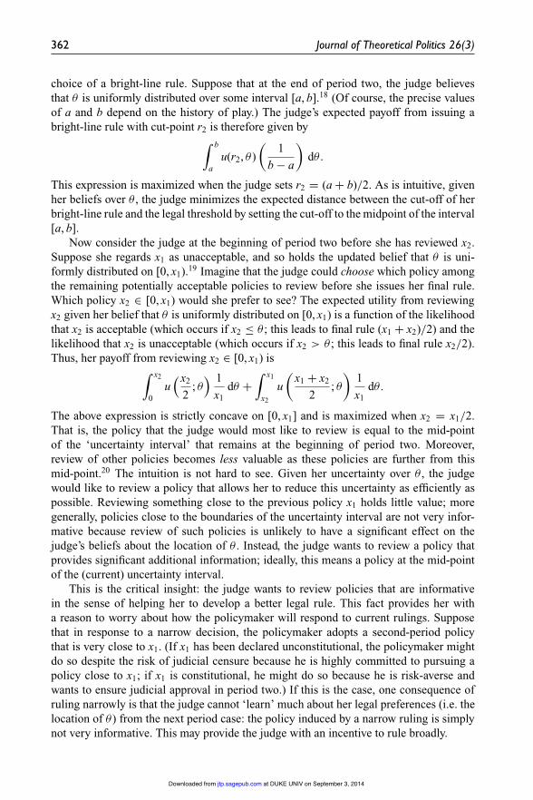
Figure 1. Classifying policies. As we move from left to right, policies become more burdensomein terms of the legally relevant criterion. Policies that are less than or equal to θ are acceptableunder the judge’s legal principle and policies that fall above θ are unacceptable.

the judge does not know the precise location of the threshold θ that divides acceptablepolicies from unacceptable policies. Formally, the judge may know that she regards poli-cies that are sufficiently ‘moderate’ as acceptable (those below some threshold a) and thatshe regards some policies as unacceptable because they are ‘too extreme’ (those abovesome threshold b > a). But she is uncertain about how she feels about policies that liebetween a and b. That is, from judge’s perspective, θ , the cut-off that separates constitu-tional from unconstitutional policies, is a random variable with support (a, b). Asked ‘inthe abstract’ whether a particular policy x ∈ (a, b) is acceptable, the judge is not sure. Butonce the judge reviews a specific policy x, and is presented with evidence and arguments,she learns whether x falls to the left (‘x is acceptable’) or right (‘x is unacceptable’) of θ ,and in doing so, learns something about the location of θ .11 For example, suppose thatthe judge reviews x and discovers that she regards it as acceptable. She has now learned θ

must lie somewhere in [x, b). Similarly, if she regards x as unacceptable, θ must lie some-where in (a, x). This modeling approach captures the intuitive notion that a judge who isunsure about the implications of her legal principles for a specific policy area becomesmore certain as she hears more and more cases. As a result, she can formulate legal ruleswith greater accuracy and confidence.12

The model consists of two periods. The restriction to two periods ensures that themodel is tractable, while preserving the dynamic that is at the heart of our argument:the judge can learn from hearing cases across the two periods, and the policymaker canrespond to first-period decisions in the second period. The critical question is whetherthere are reasons for the judge to issue a broad ruling in the first period (we make precisewhat we mean by ‘narrow’ and ‘broad’ below).

In what follows, we assume that there is an existing status quo policy, which we taketo be x = 0, and this policy has been found to be acceptable and declared constitutionalby the judge at some earlier point in time. The sequence of play is:

1. Legal threshold is drawn. Neither the policymaker nor the judge observe θ , but bothknow that θ is uniformly distributed on X = [0, 2].

2. First-period review stage. The judge reviews an (exogenously given) policy x1 ∈ X .She learns whether x1 is acceptable under her legal principle or not. The judge issuesa legal rule that declares x1 constitutional or unconstitutional, and that may (but neednot) make pronouncements on the constitutionality of other policies (we provide amore precise definition of legal rules next).




3. First-period implementation stage. If the judge’s rule declares x1 unconstitutional,policy reverts to the status quo x = 0; otherwise x = x1 is implemented.

4. Second-period policymaking stage. The policymaker, who has observed the judge’sfirst-period ruling, proposes a second-period policy x2.

5. Second-period review stage. The judge reviews policy x2, learns whether it is accept-able under her legal principle, and issues a decision that declares x2 constitutional orunconstitutional, and announces a final legal rule.

6. Second-period implementation stage. If the judge’s rule declares x2 unconstitutional,policy reverts to the current status quo (x = 0 if x1 was unconstitutional; x = x1 if x1

was constitutional). If the judge’s rule declares x2 constitutional, it is implemented.

The task for the judge is to craft legal rules. Formally, a legal rule is a function thatmaps every policy x $→ {constitutional, unconstitutional, undecided}. A special type oflegal rule is a bright-line rule. A bright-line rule announces a cut-point r ∈ X , suchthat policies above the cut-point are declared unconstitutional and policies below the cut-point are declared constitutional. The important feature of a bright-line rule is that itunambiguously classifies every policy as either constitutional or not. We assume that theultimate goal of the judge is to work towards a legal regime that provides such certainty. Inour two-period model, we capture this feature by assuming that the judge will announcea bright-line rule at the end of period two. Clearly, the judge’s most preferred bright-line rule is r = θ , which disposes of all cases in accordance with her preferences.13 Asr diverges from θ , more and more cases are disposed of incorrectly. We represent thejudge’s preferences over bright-line rules with the utility function u(r; θ ) = − | r − θ |.

We assume that in the first period, the judge is not confined to bright-line rules.Instead, she is free to issue ‘incomplete rules’. Unlike bright-line rules, incomplete rulesmake definitive statements only about a subset of policies. Specifically, suppose that inhearing a case, the judge learns that x1 is unacceptable under her legal principle andshe announces a first-period ‘incomplete rule’ r1 ∈ [0, x1]. The meaning of this rule isthat policies above r1 are declared unconstitutional (including x1), but the judge reservesjudgment on policies below r1 (that is, the rule does not declare policies below r1 consti-tutional: it leaves the status of these policies ‘undecided’). Conversely, if she learns thatx1 is acceptable, she announces a rule r1 ∈ [x1, 2] that partitions policies into those thatare constitutional (policies below r1), and those on which the judge has yet to take a stand(those above r1).14

2.1. Broad and narrow rulesWithin the set of incomplete rules, we can distinguish between broad and narrow rules.Suppose the judge wants to declare x1 constitutional. There are two types of incompleterules the judge can announce (the corresponding rules for declaring x1 unconstitutionalare symmetric):

• A narrow opinion, which sets r1 = x1;• A broad opinion, which sets r1 > x1.

The first rule is ‘narrow’ in the sense that the judge leaves all policies about which sheis still uncertain ‘undecided’, that is, the judge does not decide more than is necessary to



Fox and Vanberg 361

dispose of the first-period case correctly. To see this, note that if x1 is acceptable underthe judge’s legal principle, then by implication all x < x1 are acceptable in the judge’seyes as well, and the judge knows this.15 Thus, a narrow rule makes definite pronounce-ments only for policies about which the judge is certain. In contrast, the second typeof rule is ‘broad’ in the sense that it declares some policies constitutional about whichthe judge is still uncertain (specifically, x ∈ (x1, r1]).16 Consider how the two opinionsused as illustrative examples in the introduction fit into this modeling approach. In Quon,Kennedy’s opinion was narrow. It declared that x1 (the audit of Quon’s messages) wasconstitutional, but it explicitly refused to speculate whether other policies (i.e. searches)might raise concerns. In contrast, Scalia’s opinion in Employment Division was broad. Itannounced that x1 (withholding of benefits) was constitutional and that other restrictionsthat the Court had not yet confronted would be constitutional as well.

This formulation allows us to capture the essence of the epistemological objection tobroad opinions. Because broad opinions apply to policies the judge has not yet reviewed,they may get it wrong: a broad rule might declare as constitutional policies that thejudge would regard as unacceptable were she to review a case involving them (and viceversa). Naturally, this is only a problem if opinions are ‘sticky’; that is, if, having beenannounced, a broad rule cannot be undone costlessly in the future. We capture this finalaspect by assuming that the judge is bound by stare decisis, that is, that the second-periodrule must be consistent with the first-period rule.

Definition 1 The second-period rule is consistent with the first-period rule if all policiesdeclared unconstitutional (constitutional) under the first-period rule are also declaredunconstitutional (constitutional) under the second-period rule.

To see the implications of consistency, consider the case in which the judge’s first-period rule declares all policies weakly above r1 unconstitutional (and remains silent onall policies below r1). Then consistency requires that the judge’s second-period rule alsodeclare all policies weakly above r1 unconstitutional (and so r2 ≤ r1).17

To close out the description of the model, we must specify the player’s payoffs. Weassume that the policymaker cares about the policy implemented in the second period.Formally, if x is implemented in period two, the policymaker’s payoff is π (x; α). Thejudge cares about how closely the final legal rule approximates the rule she would craftif she had perfect information about the legal threshold. That is, given the underlyingthreshold θ and the second-period bright-line rule r2, the judge’s payoff is u(r2; θ ). Inanalyzing the model, we restrict attention to sequential equilibria (Kreps and Wilson,1982). Formal proofs of all results are in the appendix.

2.2. The informational value of casesTo develop the intuition that explains why the judge may choose to use different legalrules, and in particular, broad rules, in period one, we must begin by considering theproblem confronting the judge at the end of the game: she must craft a legal rule thatapproximates her underlying legal principles despite the fact that she is uncertain abouthow she evaluates policies she has not yet reviewed. Thus, when she chooses the finallegal rule, she must do so in light of her uncertainty about the extent to which differ-ent rules approximate the underlying legal threshold. Consider what this implies for the




choice of a bright-line rule. Suppose that at the end of period two, the judge believesthat θ is uniformly distributed over some interval [a, b].18 (Of course, the precise valuesof a and b depend on the history of play.) The judge’s expected payoff from issuing abright-line rule with cut-point r2 is therefore given by

∫ b

au(r2, θ )

(1

b − a

)dθ .

This expression is maximized when the judge sets r2 = (a + b)/2. As is intuitive, givenher beliefs over θ , the judge minimizes the expected distance between the cut-off of herbright-line rule and the legal threshold by setting the cut-off to the midpoint of the interval[a, b].

Now consider the judge at the beginning of period two before she has reviewed x2.Suppose she regards x1 as unacceptable, and so holds the updated belief that θ is uni-formly distributed on [0, x1).19 Imagine that the judge could choose which policy amongthe remaining potentially acceptable policies to review before she issues her final rule.Which policy x2 ∈ [0, x1) would she prefer to see? The expected utility from reviewingx2 given her belief that θ is uniformly distributed on [0, x1) is a function of the likelihoodthat x2 is acceptable (which occurs if x2 ≤ θ ; this leads to final rule (x1 + x2)/2) and thelikelihood that x2 is unacceptable (which occurs if x2 > θ ; this leads to final rule x2/2).Thus, her payoff from reviewing x2 ∈ [0, x1) is

∫ x2

0u(x2

2; θ

) 1x1

dθ +∫ x1

x2

u(

x1 + x2

2; θ

)1x1

dθ .

The above expression is strictly concave on [0, x1] and is maximized when x2 = x1/2.That is, the policy that the judge would most like to review is equal to the mid-pointof the ‘uncertainty interval’ that remains at the beginning of period two. Moreover,review of other policies becomes less valuable as these policies are further from thismid-point.20 The intuition is not hard to see. Given her uncertainty over θ , the judgewould like to review a policy that allows her to reduce this uncertainty as efficiently aspossible. Reviewing something close to the previous policy x1 holds little value; moregenerally, policies close to the boundaries of the uncertainty interval are not very infor-mative because review of such policies is unlikely to have a significant effect on thejudge’s beliefs about the location of θ . Instead, the judge wants to review a policy thatprovides significant additional information; ideally, this means a policy at the mid-pointof the (current) uncertainty interval.

This is the critical insight: the judge wants to review policies that are informativein the sense of helping her to develop a better legal rule. This fact provides her witha reason to worry about how the policymaker will respond to current rulings. Supposethat in response to a narrow decision, the policymaker adopts a second-period policythat is very close to x1. (If x1 has been declared unconstitutional, the policymaker mightdo so despite the risk of judicial censure because he is highly committed to pursuing apolicy close to x1; if x1 is constitutional, he might do so because he is risk-averse andwants to ensure judicial approval in period two.) If this is the case, one consequence ofruling narrowly is that the judge cannot ‘learn’ much about her legal preferences (i.e. thelocation of θ ) from the next period case: the policy induced by a narrow ruling is simplynot very informative. This may provide the judge with an incentive to rule broadly.



Fox and Vanberg 363

2.3. Pushing the policymakerThe previous section established that the judge has strict preferences over the policies shewould like to review in period two. When the judge believes that θ is uniform on [0, x1],the policy she most wants to review is x2 = x1/2; when she believes that θ is uniform on[x1, 2], it is x2 = (x1 + 2)/2. Policies decline in ‘informational value’ as they get furtherfrom these points. Of course, the judge cannot directly choose which policy to review,since only those policies that the policymaker proposes can come before the judge. Howinformative the period-two policy is therefore depends upon the policymaker’s decision.

To see the implications of this fact, consider a case in which the judge reviews x1 andfinds it unacceptable under her legal principle.21 As a result, the judge and policymakerbelieve that θ is uniform on [0, x1). Suppose the judge rules narrowly, declaring x1 andall policies above it as unconstitutional. How will the policymaker react to this decision?If the policymaker proposes a policy x2 ≥ x1, it will be declared unconstitutional. If heproposes a policy x2 < x1, it is declared constitutional if the judge finds it acceptableunder her legal principle, and declared unconstitutional otherwise (resulting in reversionto the status quo policy x = 0). The probability that the judge finds x2 ∈ [0, x1) acceptableis (x1 − x2)/x1. Thus, the policymaker’s expected utility from proposing x2 ∈ X is

{ x2x1

π (0; α) + x1−x2x1

π (x2; α), if x2 < x1

π (0; α), if x2 ≥ x1.(1)

This expected utility is maximized either at or to the left of the policymaker’s idealpoint.22 The fact that the policymaker may choose to make a proposal to the left of hisideal point stems from his concern about having the proposal declared unconstitutional:he may be willing to moderate his proposal in order to increase the likelihood of aconstitutionality ruling. In what follows, we use x∗ to denote the proposal x2 thatmaximizes (1).

We are now in a position to see why the judge may have reason to rule broadly inperiod one. Suppose that instead of ruling narrowly, she rules broadly, setting r1 < x1

(which implies that policies x2 ∈ (r1, x1) will be declared unconstitutional, even thoughthe judge, on the basis of the first period case, is not certain how she would view suchpolicies if he reviewed them). In the face of such a ruling, the policymaker knows thatproposing x2 > r1 will result in a judicial veto, something he wants to avoid. If the ruleis sufficiently broad and outlaws the policy the policymaker would adopt in response toa narrow rule (i.e. r1 < x∗), he will respond by choosing the closest ‘legal’ policy to x∗,setting x2 = r1.23

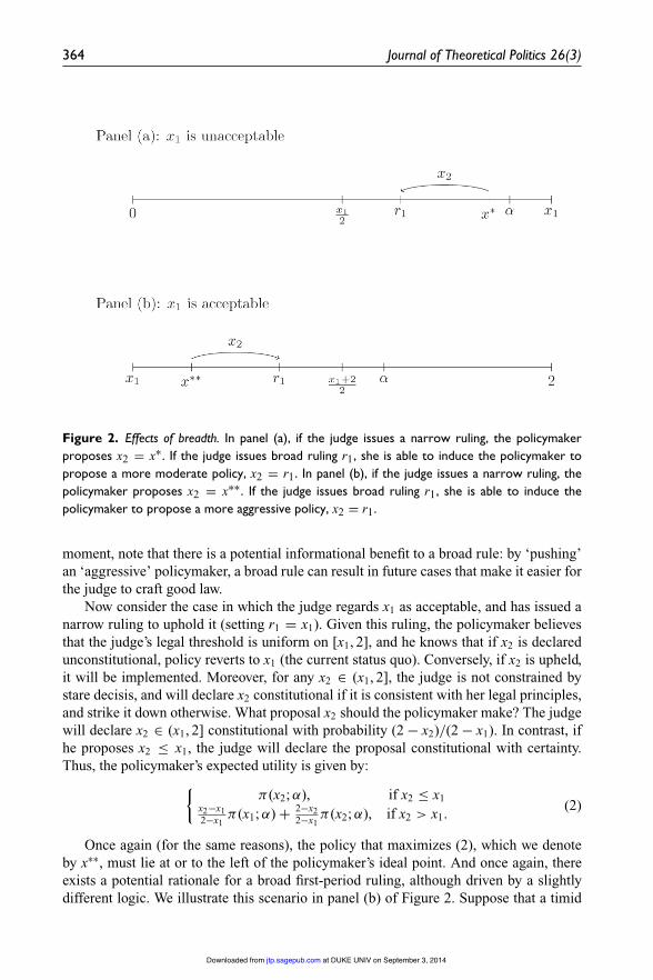
In other words, if a ruling is broad enough, the judge can induce the policymaker tomake a more moderate proposal than he would otherwise. Why might the judge want todo so? We illustrate the logic in panel (a) of Figure 2. Recall that the most informativepolicy for the judge, the policy she would most prefer to review, is x1/2. Suppose thatleft to his own devices, the policymaker will exploit the legal room created by a narrowruling to adopt a policy x∗ that is close to the one that has just been struck down. Ratherthan accept such an uninformative response, the judge can issue a broad rule to the leftof x∗ that will ‘push’ the policymaker to a more moderate, and informative, proposal.Of course, doing so has costs (these costs, which will be the focus of the next section,explain why the judge will not push the policymaker all the way to x1/2). But for the




Figure 2. Effects of breadth. In panel (a), if the judge issues a narrow ruling, the policymakerproposes x2 = x∗. If the judge issues broad ruling r1, she is able to induce the policymaker topropose a more moderate policy, x2 = r1. In panel (b), if the judge issues a narrow ruling, thepolicymaker proposes x2 = x∗∗. If the judge issues broad ruling r1, she is able to induce thepolicymaker to propose a more aggressive policy, x2 = r1.

moment, note that there is a potential informational benefit to a broad rule: by ‘pushing’an ‘aggressive’ policymaker, a broad rule can result in future cases that make it easier forthe judge to craft good law.

Now consider the case in which the judge regards x1 as acceptable, and has issued anarrow ruling to uphold it (setting r1 = x1). Given this ruling, the policymaker believesthat the judge’s legal threshold is uniform on [x1, 2], and he knows that if x2 is declaredunconstitutional, policy reverts to x1 (the current status quo). Conversely, if x2 is upheld,it will be implemented. Moreover, for any x2 ∈ (x1, 2], the judge is not constrained bystare decisis, and will declare x2 constitutional if it is consistent with her legal principles,and strike it down otherwise. What proposal x2 should the policymaker make? The judgewill declare x2 ∈ (x1, 2] constitutional with probability (2 − x2)/(2 − x1). In contrast, ifhe proposes x2 ≤ x1, the judge will declare the proposal constitutional with certainty.Thus, the policymaker’s expected utility is given by:

{π (x2; α), if x2 ≤ x1

x2−x12−x1

π (x1; α) + 2−x22−x1

π (x2; α), if x2 > x1. (2)

Once again (for the same reasons), the policy that maximizes (2), which we denoteby x∗∗, must lie at or to the left of the policymaker’s ideal point. And once again, thereexists a potential rationale for a broad first-period ruling, although driven by a slightlydifferent logic. We illustrate this scenario in panel (b) of Figure 2. Suppose that a timid



Fox and Vanberg 365

policymaker (i.e. one very concerned to avoid a judicial veto in period two) with idealpoint α > x1 reacts to a narrow ruling by proposing a policy x∗∗ that is very close to x1

(and therefore likely to be upheld). This proposal is not very informative for the judge,who would prefer to review a policy close to (x1 + 2)/2. Putting it differently, from thejudge’s perspective, the policymaker’s risk aversion leads him to hew too closely to thepolicy just upheld. By writing a broad rule with cut-off r1 > x1 (which guarantees thatall policies in the (x1, r1] interval will be declared constitutional) the judge can providereassurance that leads the policymaker to make a bolder and more informative proposalthan he otherwise would. Specifically, a broad rule r1 ∈ (x∗∗, (x1 + 2)/2] will lead a timidpolicymaker to propose x2 = min{α, r1}, which is closer to the judge’s preferred policythan x∗∗ (see the figure).24 Of course, as in the previous case, the fact that a broad rulecan induce a more informative second-period proposal does not imply that the judge willwant to rule broadly; there are potential costs to doing so, and we consider these trade-offs in the next section. Nevertheless, we have established that a broad ruling can provideinformational benefits to the judge.

2.4. The costs of breadthThere are potential gains to the judge in issuing a broad ruling in period one. But ofcourse, broad rulings also have a downside: they can generate lock-in costs. Suppose thejudge finds x1 unacceptable and issues a broad ruling r1 < x1. The policymaker willrespond to this ruling by proposing a policy within the remaining ‘legally permissible’range, that is, x2 ≤ r1. If the judge learns that she regards x2 as acceptable, she hasdiscovered that her underlying legal threshold lies between x2 and x1, and she wouldlike to set the final bright-line rule r2 = (x2 + x1)/2. Unfortunately, the requirementthat the second-period rule must be consistent with her first-period rule may preventher from being able to announce this rule whenever x2 is sufficiently close to r1 (sincewhenever x2 is close enough to r1, r1 < (x2 + x1)/2). The best the judge can do in sucha situation is to affirm the existing rule (i.e. set r2 = r1). This situation captures theepistemological objection to broad rulings: judges run the risk of being ‘locked in’ toinappropriate rules by the forces of stare decisis (or any other force that pushes themtowards legal consistency).

This, then, is the fundamental trade-off confronting judges in our model: by issuingbroad rulings, they can shape policy responses by the policymaker, and thus ensure thatthey will hear more informative cases than those that result from a narrow ruling. Butdoing so comes at the potential cost of being ‘stuck’ with legal rules that turn out to beless than ideal in light of new evidence. In short, the informational gains associated withusing judicial breadth must be weighed against the associated lock-in costs. Intuitively,how this trade-off plays out depends critically on how close the policymaker’s responseto a narrow ruling is to the previous policy x1. In other words, it depends on how ‘infor-mative’ the policymaker’s proposal is. And this, in turn, depends on the policymaker’spreferences, specifically on the policymaker’s ideal point (which policy does he wish toimplement?) and on his attitudes towards risk (how does the policymaker view the poten-tial trade-off between pursuing his policy goal and the threat of a judicial veto?). In thenext section, we turn to this issue, and provide equilibrium conditions that will lead thejudge to issue broad rulings.




3. Ruling broadly: Equilibrium conditionsAs we have just seen, the judge may have an incentive to rule broadly if the policymaker’sresponse to a narrow ruling is close to the original policy. This may occur for two rea-sons. If the judge finds the first-period policy unacceptable, it may occur because thepolicymaker is so risk-accepting in pursuing his preferred policy that he is willing toexploit the legal maneuver room left by a narrow rule to adopt a policy close to x1 despitethe risk of judicial censure. If the judge finds the first-period policy acceptable, it mayoccur because the policy-maker is so risk-averse that he adopts a policy close to x1 inhopes of securing judicial approval. What differentiates the two scenarios is that in one,the policy-maker is risk-accepting and has sufficiently extreme preferences, while in theother he is sufficiently risk-averse.

In this section, we flesh out this intuition by presenting two propositions, one thatdeals with the case in which the judge finds the first-period policy unacceptable and onethat deals with the case in which the judge finds the first-period policy acceptable. Foreach scenario, we identify the class of policymakers whose proposals are sufficientlyuninformative that ruling broadly is optimal. In particular, we allow policymakers tovary across two dimensions: their ideal point and their tolerance toward risk. In statingthe propositions, we assume without loss of generality that the exogenous first-periodpolicy x1 = 1. The first proposition covers the case in which the judge concludes thatthe first-period policy is inconsistent with her legal principles. As a result, the judge (andpolicymaker) believes that θ is uniformly distributed on [0, 1).

Proposition 1 Suppose the judge regards x1 = 1 as unacceptable, and the policymaker’sexpected utility is single-peaked on [0, min{α, 1}].25

(a) If the policymaker is risk-averse (π is strictly concave), the judge will never rulebroadly.

(b) If the judge rules broadly, the policymaker’s ideal point must be sufficientlyextreme (α > (3 +

√3)/6).

(c) If the judge issues a broad ruling, she sets r1 = 2/3.(d) If the policymaker is risk-accepting, and his ideal point satisfies (b), then

scenarios exist under which the judge rules broadly.

Consider the intuition behind part (a). Because a risk-averse policymaker is con-cerned to avoid a judicial veto, he responds to a narrow rule with a policy that is alreadyso moderate that a broad rule cannot provide informational gains to the judge. Theintuition behind part (b) is similar. Policymakers whose ideal point is moderate (i.e.α < (3 +

√3)/6) respond to a narrow ruling with a proposal that is already so different

from x1 that the informational gains of a broad ruling do not justify the associated lock-incosts. Only if the policymaker is sufficiently extreme in his preferences may the responseto a narrow ruling be so uninformative that it is beneficial to ‘push down’ the proposalwith the help of a broad ruling. Part (c) identifies which broad rule the judge will adopt;note that this rule is above the most informative policy the judge could review, and whichshe would choose to review in an ‘unconstrained’ world (x2 = 1/2). Because the judgeincurs lock-in costs for pushing down the policymaker, she chooses not to push all theway to 1/2; the informational gains of doing so do not outweigh the additional lock-incosts.



Fox and Vanberg 367

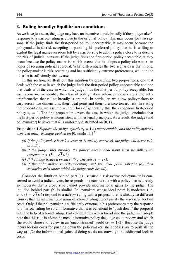
Figure 3. Class of policymakers for which breadth is optimal when x1 = 1 is unacceptable. The shadedregion indicates those values of α and λ for which the judge rules broadly, using legal breadth topush the policymaker to propose a more moderate policy. In the shaded region, the judge setsthe cut-off of her first-period rule r1 = 2/3.

Part (d) is illustrated in Figure 3. To draw this figure, we impose a specific func-tional form, assuming that the policymaker’s payoff function is given by π (x2; α, λ) =1/(| x − α | +λ), where λ > 0. This utility function (chosen largely for analyticaltractability) is risk-accepting on [0, α]. As λ decreases, the policymaker is more will-ing to bear the risk of judicial censure in pursuit of his ideal point. Put differently, as λ

decreases, the policymaker becomes more risk accepting. As a result, as λ approaches 0,the policymaker may become so aggressive in the second-period proposal that a broadruling is worthwhile. The shaded region of Figure 3 identifies those values of α and λ forwhich the judge rules broadly. Note that she issues a broad rule only if the policymaker’sideal point is sufficiently extreme (α > (3 +

√3)/6) and the policymaker is sufficiently

risk-accepting (λ is small enough); jointly, these conditions ensure that the response to anarrow ruling is so close to x1 that a broad ruling is optimal.26

We now turn to the case in which the judge concludes that the first-period policy isacceptable, which implies that the judge (and policymaker) believes that θ is uniformlydistributed on [1, 2].




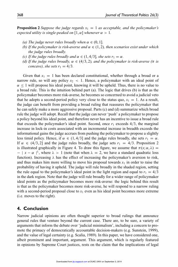
Proposition 2 Suppose the judge regards x1 = 1 as acceptable, and the policymaker’sexpected utility is single-peaked on [1, α] whenever α > 1.

(a) The judge never rules broadly when α ∈ (0, 1].(b) If the policymaker is risk-averse and α ∈ (1, 2), then scenarios exist under which

the judge rules broadly.(c) If the judge rules broadly and α ∈ (1, 4/3], she sets r1 = α.(d) If the judge rules broadly, α ∈ (4/3, 2), and the policymaker is risk-averse (π is

concave), she sets r1 = 4/3.

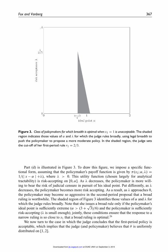
Given that x1 = 1 has been declared constitutional, whether through a broad or anarrow rule, so will any policy x2 < 1. Hence, a policymaker with an ideal point ofα ≤ 1 will propose his ideal point, knowing it will be upheld. Thus, there is no value toa broad rule. This is the intuition behind part (a). The logic that drives (b) is that as thepolicymaker becomes more risk-averse, he becomes so concerned to avoid a judicial vetothat he adopts a second-period policy very close to the status quo, x1 = 1. As a result,the judge can benefit from providing a broad ruling that reassures the policymaker thathe can safely make a more aggressive proposal. Parts (c) and (d) summarize which broadrule the judge will adopt. Recall that the judge can never ‘push’ a policymaker to proposea policy beyond his ideal point, and therefore never has an incentive to issue a broad rulethat exceeds the policymaker’s ideal point. Second, once r1 exceeds 4/3, the marginalincrease in lock-in costs associated with an incremental increase in breadth exceeds theinformational gains the judge accrues from pushing the policymaker to propose a slightlyless timid policy. Hence, if α ∈ (1, 4/3] and the judge rules broadly, she sets r1 = α.If α ∈ (4/3, 2] and the judge rules broadly, the judge sets r1 = 4/3. Proposition 2is illustrated graphically in Figure 4. To draw this figure, we assume that π (x; α, λ) =− | x − α |λ, where λ > 1 (note that when λ = 2, we have a standard quadratic lossfunction). Increasing λ has the effect of increasing the policymaker’s aversion to risk,and thus makes him more willing to move his proposal towards x1 in order to raise theprobability of having it upheld. The judge will rule broadly in the shaded region, settingthe rule equal to the policymaker’s ideal point in the light region and equal to r1 = 4/3in the dark region. Note that the judge will rule broadly for a wider range of policymakerideal points as the policymaker becomes more risk-averse: the logic behind this resultis that as the policymaker becomes more risk-averse, he will respond to a narrow rulingwith a second-period proposal close to x1 even as his ideal point becomes more extreme(i.e. moves to the right).

4. ConclusionNarrow judicial opinions are often thought superior to broad rulings that announcegeneral rules that venture beyond the current case. There are, to be sure, a variety ofarguments that inform the debate over ‘judicial minimalism’, including a concern to pro-mote the primacy of democratically accountable decision-makers (e.g. Sunstein, 1999),and the value of legal certainty (e.g. Scalia, 1989). In this paper, we have considered one,albeit prominent and important, argument. This argument, which is regularly featuredin opinions by Supreme Court justices, rests on the claim that the implications of legal



Fox and Vanberg 369

Figure 4. Class of policymakers for which breadth is optimal when x1 = 1 is acceptable. The shadedregion indicates those values of α and λ for which the judge rules broadly, using legal breadth toinduce the policymaker to propose a more aggressive policy. In the light region, the judge setsthe cut-off of her first-period rule equal to the ideal point of the policymaker, that is, r1 = α, andin the dark region, the judge sets the cut-off of her first-period rule r1 = 4/3.

principles for particular policies and cases are often difficult to ascertain in the abstract.Especially where competing values must be balanced, judges may only know what thelegal principles to which they are committed demand when they adjudicate a particulardispute. As a result, judges risk error when they announce general rules that apply tocircumstances or policies with which they have not yet been confronted. In light of suchuncertainty, the argument goes, narrow opinions are desirable because they limit judicialerror.

We have challenged this argument. The intuition underlying the claim we make issimple. At least when judges rule on the constitutionality of the policies adopted bylegislators and bureaucrats, judicial decisions shape the legal landscape by defining whatis legally (im)permissible. As a result, current decisions affect the policies that will beadopted in the future. And because only those policies that are actually adopted can bechallenged, current decisions affect the subsequent cases that judges will hear. As wehave shown, in this dynamic setting, judicial uncertainty about the policy implications oflegal principles may, in contrast to conventional arguments, provide a reason for judicialbreadth rather than minimalism by allowing the court to guide the policy responses ofoverly ‘aggressive’ or ‘timid’ policymakers. Another way to put the point is to say that the




epistemological argument for judicial minimalism focuses on one consequence of limitedjudicial knowledge: the desire to avoid mistakes. Our argument highlights that, as withmost things in life, there is a trade-off: narrow rulings prevent the adoption of legal rulesthat turn out to be inappropriate ex post. But if current decisions shape future policies,then narrow rules may also lead policymakers to respond to decisions with policies thatprovide judges with little useful information in crafting ‘good’ legal rules. Broad rulingsthat ‘push’ policymakers can help judges to develop legal rules that more accuratelyreflect their legal principles.

In closing, several caveats are worth noting. The first emerges from the last point.Our argument rests squarely on the fact that current decisions shape policy responsesand therefore future cases. Although this assumption is plausible, especially when judgesrule on public policies that are likely to be revised in light of judicial decisions, it is worthemphasizing that our argument does not apply if the issues brought before the court inthe future are independent of current decisions. A second caveat is closely connected.We should be clear that the central thrust of our argument is not explanatory. We are notclaiming that in choosing between a narrow and a broad approach to decisions, judgesare primarily concerned with influencing public policy responses in an effort to gener-ate ‘informative’ future cases.27 Rather, the aim of the argument is to demonstrate thata prominent normative argument in favor of narrow opinions, the epistemological objec-tion, is insufficient to establish that broad opinions are undesirable. Judicial ignoranceis not always an argument for narrowness; judges with limited knowledge may, in fact,want to write broad opinions in order to confront their uncertainty.

A final point concerns the restriction of our model to two periods. In part, our conclu-sions are driven by the fact that the judge in our model is ‘stuck’ with the second-periodrule. As a result, she is eager to use the first-period rule to learn as much as possible abouther preferences. This leads her (sometimes) to rule broadly. To take the polar oppositeof our model, imagine an infinitely patient judge confronting an infinite series of cases(and policies). She would have no reason to rule broadly, since she can adjust the legalrule piecemeal over time, and (because she is infinitely patient) is content to work slowlytowards the ideal rule, taking no risks in ruling broadly. Clearly, our argument does notapply to this judge. In the ‘real world’, of course, judges fall somewhere between thesepoles. On the one hand, there are multiple, recurring opportunities to refine legal rules,and judges therefore do not face the same pressures as the judge in our model. On theother hand, judges do face time pressures. Some policy areas provide only infrequentopportunities to revise the law. More importantly, judges are not likely to be infinitelypatient in developing ‘good’ legal rules. They know that they must eventually leave thebench. Moreover, frequent revision of a rule reduces legal certainty and imposes reliancecosts on individuals who must make decisions in light of the currently prevailing rule. Asa result, judges will feel some urgency to arrive at a ‘good’ legal rule. And if this is true,the trade-off we have identified rears its head.

AppendixRecall the definition of s in endnote 11. This appendix considers the case in whichthe judge concludes that the rst-period policy x1 = 1 is unacceptable (s1 = unac-ceptable). Appendix A.1 deals with the incentives confronting the judge in the second



Fox and Vanberg 371

period. Appendix A.2 deals with the incentives confronting the policymaker in the sec-ond period. Appendix A.3 deals with the incentives confronting the judge in the firstperiod. Appendix A.4 formally proves Proposition 1 using the results from AppendixA.1, A.2 and A.3. The proof of Proposition 2 is proved in an analogous manner and isavailable upon request.

Given that the judge has concluded that x1 = 1 is unacceptable, the density of thejudge’s posterior belief about θ at the time she issues her first-period ruling is equal toone for all θ ∈ [0, 1). Further, we assume that in the first period, the judge either issuesa narrow ruling r1 = 1 that declares x1 = 1 and all policies above x1 = 1 as unconstitu-tional, or a broad ruling r1 ∈ [0, 1) that declares all policies x > r1 as unconstitutional.Finally, recall that we restrict the judge to using a bright-line rule r2 in the second period.Such a rule declares all policies x < r2 as constitutional and all policies x > r2 as uncon-stitutional. How the rule treats policy x = r2 is not pinned down by the definition in themain text. For technical convenience, we assume that whenever r2 < 1, policy x = r2 isdeclared constitutional.

A.1. The judge’s second-period problemWrite U(r2; a, b) for the judge’s expected payoff from issuing a bright-line rule with cut-off r2 when the density of the distribution of θ is equal to 1/(b − a) for all θ ∈ (a, b).Hence,

U(r2; a, b) =∫ b

au(r2; θ )

1b − a

dθ .

Fact 1. Suppose 0 ≤ a < b ≤ 2. Then U(·; a, b) is single-peaked in r2 on [0, 2] and isstrictly maximized when r2 = (a + b)/2.

Proof: Using the fact that u(r2; θ ) = − | r2 − θ |, we have that

U(r2; a, b) =

⎧⎪⎨

⎪⎩

− a+b2 + r2, if r2 ≤ a

−a2−b2+2(a+b)r2−2r22

2(b−a) , if a < r2 < ba+b

2 − r2, if r2 ≥ b.

Hence,

∂U∂r2

(r2; a, b) =

⎧⎨

⎩

1, if r2 < a(b+a)−2r2

(b−a) , if a < r2 < b−1, if r2 > b.

Inspection reveals that for all r2 ∈ (0, a) ∪ (a, (a + b)/2), ∂U/∂r2(r2; a, b) > 0, andfor all r2 ∈ ((a + b)/2, b) ∪ (b, 2), ∂U/∂r2(r2; a, b) < 0. These facts, together with thecontinuity of U(·; a, b) in r2 on [0, 2] imply that U(·; a, b) is single-peaked on [0, 2] andis strictly maximized when r2 = (a + b)/2. !

Our requirement that the judge’s second-period rule is consistent with her first-periodrule implies that the cut-off of her second-period rule r2 ≤ r1. In light of this fact, wehave the following lemma.




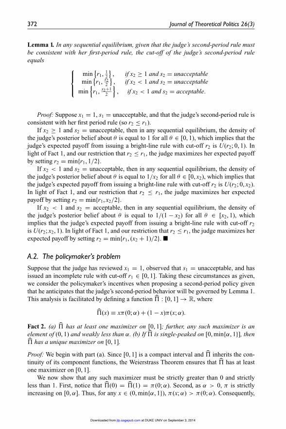
Lemma 1. In any sequential equilibrium, given that the judge’s second-period rule mustbe consistent with her first-period rule, the cut-off of the judge’s second-period ruleequals

⎧⎪⎨

⎪⎩

min{r1, 1

2

}, if x2 ≥ 1 and s2 = unacceptable

min{r1, x2

2

}, if x2 < 1 and s2 = unacceptable

min{

r1, x2+12

}, if x2 < 1 and s2 = acceptable.

Proof: Suppose x1 = 1, s1 = unacceptable, and that the judge’s second-period rule isconsistent with her first period rule (so r2 ≤ r1).

If x2 ≥ 1 and s2 = unacceptable, then in any sequential equilibrium, the density ofthe judge’s posterior belief about θ is equal to 1 for all θ ∈ [0, 1), which implies that thejudge’s expected payoff from issuing a bright-line rule with cut-off r2 is U(r2; 0, 1). Inlight of Fact 1, and our restriction that r2 ≤ r1, the judge maximizes her expected payoffby setting r2 = min{r1, 1/2}.

If x2 < 1 and s2 = unacceptable, then in any sequential equilibrium, the density ofthe judge’s posterior belief about θ is equal to 1/x2 for all θ ∈ [0, x2), which implies thatthe judge’s expected payoff from issuing a bright-line rule with cut-off r2 is U(r2; 0, x2).In light of Fact 1, and our restriction that r2 ≤ r1, the judge maximizes her expectedpayoff by setting r2 = min{r1, x2/2}.

If x2 < 1 and s2 = acceptable, then in any sequential equilibrium, the density ofthe judge’s posterior belief about θ is equal to 1/(1 − x2) for all θ ∈ [x2, 1), whichimplies that the judge’s expected payoff from issuing a bright-line rule with cut-off r2

is U(r2; x2, 1). In light of Fact 1, and our restriction that r2 ≤ r1, the judge maximizes herexpected payoff by setting r2 = min{r1, (x2 + 1)/2}. !

A.2. The policymaker’s problemSuppose that the judge has reviewed x1 = 1, observed that s1 = unacceptable, and hasissued an incomplete rule with cut-off r1 ∈ [0, 1]. Taking these circumstances as given,we consider the policymaker’s incentives when proposing a second-period policy giventhat he anticipates that the judge’s second-period behavior will be governed by Lemma 1.This analysis is facilitated by defining a function &̂ : [0, 1] → R, where

&̂(x) ≡ xπ (0; α) + (1 − x)π (x; α).

Fact 2 . (a) &̂ has at least one maximizer on [0, 1]; further, any such maximizer is anelement of (0, 1) and weakly less than α. (b) If &̂ is single-peaked on [0, min{α, 1}], then&̂ has a unique maximizer on [0, 1].

Proof: We begin with part (a). Since [0, 1] is a compact interval and &̂ inherits the con-tinuity of its component functions, the Weierstrass Theorem ensures that &̂ has at leastone maximizer on [0, 1].

We now show that any such maximizer must be strictly greater than 0 and strictlyless than 1. First, notice that &̂(0) = &̂(1) = π (0; α). Second, as α > 0, π is strictlyincreasing on [0, α]. Thus, for any x ∈ (0, min{α, 1}), π (x; α) > π (0; α). Consequently,



Fox and Vanberg 373

for any x ∈ (0, min{α, 1}), &̂(x) > &̂(0) = &̂(1) = π (0; α). Thus, neither 0 nor 1 aremaximizers of &̂ on [0, 1].

We now show that any maximizer of &̂ on [0, 1] is weakly less than α. In the eventthat α ≥ 1, the result is immediate. So consider the case in which α < 1 and supposethat x ∈ (α, 1]. We need to show that &̂(α) > &̂(x):

απ (0; α) + (1 − α)π (α; α) > xπ (0; α) + (1 − x)π (x; α).

As α is the unique maximizer of π , π (α; α) > π (x; α), and π (α; α) > π (0; α). Thesefacts, together with the fact that x > α, ensure that the displayed inequality holds.Consequently, x > α cannot be a maximizer of &̂ on [0, 1].

We now turn to part (b). Suppose &̂ is single-peaked on [0, min{α, 1}], and begin byconsidering the case in which α ≥ 1. Thus, &̂ is single-peaked on [0, 1], and so has aunique maximizer on [0, 1]. Now consider the case in which α < 1. Thus, &̂ is single-peaked on [0, α], and so has a unique maximizer on [0, α]. This fact, together with part(a), ensures that &̂ has a unique maximizer on [0, 1]. !

For the remainder of the appendix, we will assume that &̂ is single-peaked on[0, min{α, 1}].

Assumption 1 . &̂ is single-peaked on [0, min{α, 1}].

In light of Fact 2(b), whenever Assumption 1 holds, &̂ has a unique maximizer on[0, 1], which we shall denote by x∗.

Lemma 2 . (a) Suppose the judge issues a narrow rule in period one. Then, in any sequen-tial equilibrium, the policymaker’s expected payoff from proposing policy x2, denoted&n

u(x2), is

&nu(x2) =

{&̂(x2), if x2 < 1π (0; α), if x2 ≥ 1.

(b) Suppose the judge issues a broad rule with breadth r1 ∈ [0, 1) in period one. Then, inany sequential equilibrium, the policymaker’s expected payoff from proposing policy x2,denoted &b

u(x2; r1), is

&bu(x2; r1) =

{&̂(x2), if x2 ≤ r1

π (0; α), if x2 > r1.

Proof: Suppose that the judge has reviewed x1 = 1 and observed that s1 = unacceptable.Then, in any sequential equilibrium, the density of the policymaker’s posterior beliefabout θ is equal to 1 for all θ ∈ [0, 1), and the judge’s behavior in the second period isgoverned by Lemma 1.

With this in mind, begin with part (a): consider the case in which the judge hasruled narrowly in period one. That is, she declares x = 1 and all policies above it asunconstitutional. The fact that x1 = 1 is unconstitutional under the judge’s first-periodrule means that the status quo remains at x = 0. Consequently, if the policymaker’ssecond-period proposal is declared unconstitutional, policy x = 0 is implemented. Fur-thermore, consistency of the judge’s second-period rule with her first-period rule requires




that the judge’s second-period rule declare all policies weakly above x = 1 as unconsti-tutional. Hence, the policymaker’s payoff from proposing a policy x2 ≥ 1 equals π (0; α).In contrast, if the policymaker proposes a policy x2 ∈ [0, 1), it will be declared con-stitutional if s2 = acceptable and will be declared unconstitutional if s2 = unacceptable(Lemma 1). Given the policymaker’s beliefs, the probability that s2 = acceptable is 1−x2

and the probability that s2 = unacceptable is x2. Hence, the policymaker’s expected pay-off from proposing x2 ∈ [0, 1) equals &̂(x2). The proof of part (b) is similar to that ofpart (a). !

The above lemma taken together with next two lemmas jointly establish that regard-less of whether the judge rules narrowly or broadly in period one, the policymaker hasan optimal proposal. Furthermore, they establish that by increasing the breadth of herfirst-period ruling, the judge can induce the policymaker to propose a policy closer to thestatus quo (x = 0) than he would otherwise propose.

Lemma 3 . Suppose Assumption 1 holds, and denote the unique value of x2 that maxi-mizes &̂ on [0, 1] as x∗. Then the value of x2 that strictly maximizes &n

u on [0, 2] equalsx∗.

Proof: Suppose Assumption 1 holds: &̂ is single-peaked on [0, min{α, 1}]. Further,denote the unique value of x2 that maximizes &̂ on [0, 1] as x∗. Fact 2(a) informs usthat x∗ ∈ (0, 1).

As x∗ ∈ (0, 1), &̂(x∗) > &̂(0) = π (0; α). Further, since x∗ < 1, &nu(x∗) = &̂(x∗).

These facts, together with the fact that &nu(x) = π (0; α) for all x > 1, imply that any

maximizer of &nu on [0, 2] is an element of [0, 1]. This fact, together with the fact that

&nu(x) = &̂(x) for all x ∈ [0, 1], implies that the set of maximizers of &n

u on [0, 2] isequivalent to the set of maximizers of &̂ on [0, 1]. Consequently, the fact that x = x∗ isthe unique maximizer of &̂ on [0, 1] implies that x = x∗ is the unique maximizer of &n

uon [0, 2]. !Lemma 4 . Suppose Assumption 1 holds, and denote the unique value of x2 that maxi-mizes &̂ on [0, 1] as x∗. If r1 ∈ (0, 1), the value of x2 that strictly maximizes &b

u(·; r1)equals

{x∗, if x∗ ≤ r1

r1, if x∗ > r1.

If r1 = 0, any value of x2 maximizes &bu(·; r1).

Proof: First, suppose that r1 ∈ (0, 1). Further, suppose Assumption 1 holds: &̂ is single-peaked on [0, min{α, 1}]. Denoting the unique maximizer of &̂ on [0, 1] by x∗, Fact 2(a)informs us that x∗ ∈ (0, 1) and that x∗ ≤ α.

Begin with the case in which x∗ ≤ r1. As x∗ ∈ (0, 1), &̂(x∗) > &̂(0) = π (0; α).Further, since x∗ ≤ r1, &b

u(x∗) = &̂(x∗). These facts, together with the fact that&b

u(x; r1) = π (0; α) for all x > r1, imply that any maximizer of &bu on [0, 2] is an

element of [0, r1]. Given that &b(x; r1) = &̂(x) on [0, r1], it thus follows that the set ofmaximizers of &b

u on [0, 2] is equivalent to the set of maximizers of &̂ on [0, r1]. Sincex = x∗ is the unique maximizer of &̂ on [0, 1], our supposition that x∗ ≤ r1 implies thatx = x∗ is the unique maximizer of &̂ on [0, r1]. Hence, x = x∗ is the unique maximizerof &b

u on [0, 2].



Fox and Vanberg 375

Now consider the case in which r1 ∈ (0, x∗). Since x∗ ≤ α, it follows that r1 ∈(0, α). This fact, together with the fact that π is strictly increasing on [0, α] implies thatπ (r1; α) > π (0; α). Given that r1 ∈ (0, 1), we can thus conclude that &̂(r1) > π (0; α).This fact, together with the fact that &b

u(r1; r1) = &̂(r1) and the fact that &bu(x; r1) =

π (0; α) for all x > r1, implies that any maximizer of &bu on [0, 2] is an element of [0, r1].

This fact, together with the fact that &bu(x; r1) = &̂(x) for all x ∈ [0, r1], implies that the

set of maximizers of &bu on [0, 2] is equivalent to the set of maximizers of &̂ on [0, r1].

Since &̂ is single-peaked around x∗ over the interval [0, min{α, 1}], our supposition thatr1 < x∗ implies that the unique maximizer of &̂ on [0, r1] is x = r1. Hence, x = r1 is theunique maximizer of &b

u on [0, 2].Finally, consider the case in which r1 = 0. Then inspection of &b

u reveals that it isinvariant in x2 and so any value of x2 is a maximizer. !

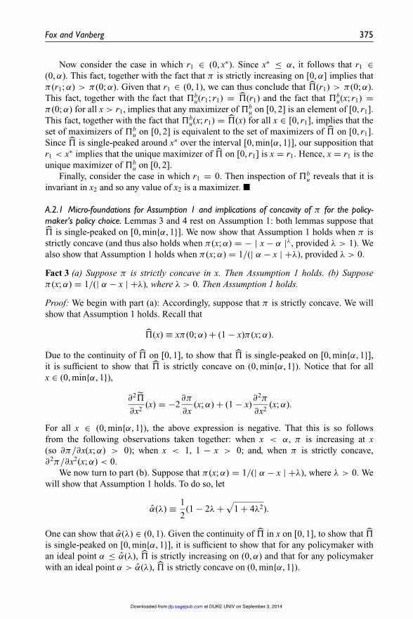
A.2.1 Micro-foundations for Assumption 1 and implications of concavity of π for the policy-maker’s policy choice. Lemmas 3 and 4 rest on Assumption 1: both lemmas suppose that&̂ is single-peaked on [0, min{α, 1}]. We now show that Assumption 1 holds when π isstrictly concave (and thus also holds when π (x; α) = − | x − α |λ, provided λ > 1). Wealso show that Assumption 1 holds when π (x; α) = 1/(| α − x | +λ), provided λ > 0.

Fact 3 (a) Suppose π is strictly concave in x. Then Assumption 1 holds. (b) Supposeπ (x; α) = 1/(| α − x | +λ), where λ > 0. Then Assumption 1 holds.

Proof: We begin with part (a): Accordingly, suppose that π is strictly concave. We willshow that Assumption 1 holds. Recall that

&̂(x) ≡ xπ (0; α) + (1 − x)π (x; α).

Due to the continuity of &̂ on [0, 1], to show that &̂ is single-peaked on [0, min{α, 1}],it is sufficient to show that &̂ is strictly concave on (0, min{α, 1}). Notice that for allx ∈ (0, min{α, 1}),

∂2&̃

∂x2(x) = −2

∂π

∂x(x; α) + (1 − x)

∂2π

∂x2(x; α).

For all x ∈ (0, min{α, 1}), the above expression is negative. That this is so followsfrom the following observations taken together: when x < α, π is increasing at x(so ∂π/∂x(x; α) > 0); when x < 1, 1 − x > 0; and, when π is strictly concave,∂2π/∂x2(x; α) < 0.

We now turn to part (b). Suppose that π (x; α) = 1/(| α − x | +λ), where λ > 0. Wewill show that Assumption 1 holds. To do so, let

α̂(λ) ≡ 12

(1 − 2λ +√

1 + 4λ2).

One can show that α̂(λ) ∈ (0, 1). Given the continuity of &̂ in x on [0, 1], to show that &̂

is single-peaked on [0, min{α, 1}], it is sufficient to show that for any policymaker withan ideal point α ≤ α̂(λ), &̂ is strictly increasing on (0, α) and that for any policymakerwith an ideal point α > α̂(λ), &̂ is strictly concave on (0, min{α, 1}).




Letting ξ (x) ≡ x2 + α + λ − 2x(α + λ), note that for any x ∈ (0, min{α, 1}),

∂&̂

∂x(x) = ξ (x)

(α + λ)(α + λ − x)2,

and that

∂2&̂

∂x2(x) = −2(α + λ − 1)

(α + λ − x)3.

Begin by supposing that α ≤ α̂(λ), which together with our restriction to policy-makers with positive ideal points implies that α ∈ (0, α̂(λ)]. We need to show that∂&̂/∂x(x) > 0 for all x ∈ (0, α). Notice that ∂&̂/∂x(x) > 0 for all x ∈ (0, α) if and onlyif ξ (x) > 0 for all x ∈ (0, α). Since ξ is strictly decreasing in x on [0, α], to show that∂&̂/∂x(x) > 0 for all x ∈ (0, α), it is sufficient to show that ξ (α) ≥ 0. Notice that ξ (α) is

strictly concave in α and is equal to 0 if and only if α =(

1 − 2λ −√

1 + 4λ2)

/2 < 0

or α = α̂(λ). This fact, together with our supposition that α ∈ (0, α̂(λ)], implies that ξ (α)is non-negative.

Now consider the case in which α > α̂(λ). We need to show that for all x ∈(0, min{α, 1}), ∂2&̂/∂x2(x) < 0. To prove this claim, it is sufficient to show that α+λ > 1.

Now notice α̂(λ) + λ =(

1 +√

1 + 4λ2)

/2 > 1. And since α > α̂(λ), it follows thatα + λ > 1. !

Fact 4 . Suppose π is strictly concave. Any maximizer x∗ of &̂ on [0, 1] is weakly less than1/2.

Proof: Suppose π is strictly concave. We know from Fact 2(a) that any maximizer of &̂ on[0, 1] is an element of (0, 1) and weakly less than α. So if α ≤ 1/2, it immediately followsthat any maximizer of &̂ on [0, 1] is weakly less than 1/2. Now consider the case in whichα > 1/2. The strict concavity of π implies that &̂ is strictly concave on (0, min{α, 1})(see the proof of part (a) of Fact 3). Consequently, to show that any maximizer of &̂ on[0, 1] is weakly less than 1/2, it is sufficient to show that ∂&̂/∂x (1/2) ≤ 0. As

∂&̂

∂x

(12

)= π (0; α) − π

(12

; α)

+ 12

∂π

∂x

(12

; α)

,

∂&̂/∂x (1/2) ≤ 0 if and only if

∂π

∂x

(12

; α)

≤π

( 12 ; α

)− π (0; α)

12 − 0

.

The strict concavity and differentiability of π in x, together with Theorem 7.9 ofSundaram (1996, p. 183), ensures that the above inequality holds. !

A.3. The judge’s first-period problemWe will use the following fact throughout this section.



Fox and Vanberg 377

Fact 5 . Suppose 0 ≤ a < b ≤ 2. The expression∫ b

a u(r; θ )dθ is single-peaked in r on[0, 2] and is strictly maximized when r = (a + b)/2.

Proof: Apply a proof technique similar to that used to prove Fact 1. !Suppose that the judge has reviewed x1 = 1 and observed that s1 = unacceptable.

Write V nu for the judge’s expected payoff from ruling narrowly (i.e. issuing an incomplete

rule that declares all policies weakly above x1 = 1 as unconstitutional), and write V bu (r1)

for the judge’s expected payoff from ruling broadly (i.e. issuing an incomplete rule witha cut-off r1 < 1 in which all policies strictly above r1 are declared unconstitutional).Throughout this section, we will assume that Assumption 1 is satisfied. This implies thatthe policymaker’s response to the judge’s first-period ruling is governed by Lemmas 3and 4. As before, we shall let x∗ denote the unique maximizer of &̂ on [0, 1]. Finally, weassume that the judge incurs an infinitesimal cost if she issues a broad ruling. In whatfollows, we will denote this cost by ε, where ε > 0. This assumption ensures that foralmost all parameterizations of our model, there will be at most one first-period rulingthat is consistent with equilibrium behavior for the judge.

Lemma 5 . Suppose that Assumption 1 holds. Then in any sequential equilibrium, wehave the following:

(a) The judge’s expected payoff from issuing a narrow ruling:

V nu ≡

∫ x∗

0u(

x∗

2; θ

)dθ +

∫ 1

x∗u(

x∗ + 12

; θ)

dθ .

(b) The judge’s expected payoff from issuing a broad ruling with breadth r1 ∈ [0, 1) is

V bu (r1) =

⎧⎪⎪⎨

⎪⎪⎩

∫ r10 u

( r12 ; θ

)dθ +

∫ 1r1

u (r1; θ ) dθ − ε, if r1 < x∗∫ x∗

0 u(

x∗2 ; θ

)dθ +

∫ 1x∗ u (r1; θ ) dθ − ε, if x∗ ≤ r1 < x∗+1

2∫ x∗

0 u(

x∗2 ; θ

)dθ +

∫ 1x∗ u

(x∗+1

2 ; θ)

dθ − ε, if x∗+12 ≤ r1.

Proof: We begin by proving part (a). Suppose that the judge has (i) reviewed x1 = 1,(ii) observed that s1 = unacceptable, (iii) has issued a narrow first-period ruling, and (iv)Assumption 1 is satisfied. Notice that (i) and (ii) imply that in any sequential equilibrium,the density of the judge’s posterior belief about θ is equal to 1 for all θ ∈ [0, 1). Giventhe judge’s beliefs, establishing part (a) amounts to establishing that the judge’s payofffor any θ < x∗ is u (x∗/2; θ ) and the judge’s payoff for any θ ≥ x∗ is u ((x∗ + 1)/2; θ ).

Given (iv) and Lemma 3, the policymaker responds to a narrow first-period rulingby proposing x∗. As such, Lemma 1 ensures that in the event that s2 = unacceptable,the judge issues a second-period ruling with cut-off x∗/2, and in the event that s2 =acceptable, the judge issues a second-period ruling with cut-off (x∗ + 1)/2. Since s2 =unacceptable whenever θ < x∗, for any θ < x∗, the judge’s payoff is u (x∗/2; θ ); and sinces2 = acceptable whenever θ ≥ x∗, for any θ ≥ x∗, the judge’s payoff is u ((x∗ + 1)/2; θ ).Hence, part (a) follows. Part (b) is proved in an analogous manner. !




Write V netu (r1; x∗) for the judge’s net benefit from issuing a broad ruling with breadth

r1 ∈ [0, 1) when a narrow ruling elicits x∗. Thus,

V netu (r1; x∗) = V b

u (r1) − V nu

Notice that V netu (·; x∗) inherits the continuity of V b

u in r1.

Fact 6 . (a) For all r1 ≥ x∗, V netu (r1; x∗) < 0. (b) V net

u (r1; x∗) ≥ 0 only if x∗ > (3 +√

3)/6.

Proof: We begin with part (a). Suppose that r1 ≥ x∗. We need to show thatV net

u (r1; x∗) < 0. First, consider the case in which r1 ∈ [(x∗ + 1)/2, 1). In light ofLemma 5, V net

u (r1; x∗) = −ε < 0. Now consider the case in which r1 ∈ [x∗, (x∗ + 1)/2).In light of Lemma 5,

V netu (r1; x∗) =

∫ 1

x∗u (r1; θ ) dθ −

∫ 1

x∗u(

x∗ + 12

; θ)

dθ − ε,

which is negative, as∫ 1

x∗ u ((x∗ + 1)/2; θ ) dθ >∫ 1

x∗ u (r1; θ ) dθ (Fact 5) and ε > 0.We now turn to part (b). For all r1 ∈ (0, x∗),

∂V netu (r1; x∗)∂r1

= ∂V bu (r1; x∗)∂r1

= 2 − 3r1

2

and

∂2V netu (r1; x∗)

∂r21

= ∂V bu (r1; x∗)∂r1

= −32

,

the latter of which implies that V bu (·; x∗) is strictly concave in r1 on (0, x∗).

Suppose that x∗ ≤ 2/3. Then ∂V netu /∂r1(r1; x∗) > 0 for all r1 ∈ (0, x∗). This fact,

together with the continuity of V netu (·; x∗) in r1 on [0, 1) and part (a) of this lemma, implies

that V netu (r1; x∗) < 0 for all r1 ∈ [0, 1). Consequently, if V net

u (r1; x∗) ≥ 0, then x∗ > 2/3.Now suppose that x∗ > 2/3. Then r1 = 2/3 is the unique solution to the first-order

condition

∂V netu (r1; x∗)∂r1

= 0

on (0, x∗). This fact, together with the fact that V netu (·; x∗) is strictly concave in r1 on (0, x∗)

and continuous in r1 on [0, x∗), implies that the value of r1 that maximizes the judge’s netbenefit of ruling broadly on [0, x∗) is r1 = 2/3. This fact, together with part (a), impliesthat V net

u (r1; x∗) ≥ 0 only if

V netu

(23

; x∗)

= 112

(1 − 6x∗(1 + x∗)) − ε ≥ 0.

As ε > 0, the above inequality holds only if x∗ > (3 +√

3)/6. !



Fox and Vanberg 379

A.4. Proof of Proposition 1Before proving Proposition 1 of the main text, we restate it in slightly more technicalterms.

Proposition 1 Suppose Assumption 1 holds and consider a sequential equilibrium.Further, suppose that the judge regards x1 = 1 as unacceptable (s1 = unacceptable).

(a) If the policymaker is risk-averse (π is strictly concave), the judge will never rulebroadly.

(b) If the judge rules broadly, the policymaker’s ideal point must be sufficiently

extreme(α > (3 +

√3)/6

).

(c) If the judge issues a broad ruling, she sets r1 = 2/3.(d) If the policymaker is risk-accepting, and his ideal point satisfies (b), then

scenarios exist under which the judge rules broadly.

Proof: Suppose that Assumption 1 holds and consider a sequential equilibrium. Further,suppose that the judge regards x1 = 1 as unacceptable (s1 = unacceptable).

Begin with part (a). Suppose π is strictly concave, and, by way of contradiction,suppose that the judge issues a broad ruling. Thus, there exists a value of r1 ∈ [0, 1) suchthat V net

u (r1; x∗) ≥ 0. A necessary condition for this inequality to hold is x∗ > (3 +√

3)/6(Fact 6(b)). However, since π is strictly concave, it follows that x∗ ≤ 1/2 (Fact 4), whichyields a contradiction.

Now turn to part (b). If the judge issues a broad ruling, then there exists a value ofr1 ∈ [0, 1) such that V net

u (r1; x∗) ≥ 0. In light of Fact 6(b), this condition is satisfied onlyif x∗ > (3 +

√3)/6. This fact, together with the fact that x∗ ≤ α (Fact 2(a)), implies that

α > (3 +√

3)/6 in any equilibrium in which the judge rules broadly.Now consider part (c). Suppose the judge rules broadly. Then there exists a value of

r1 ∈ [0, 1) such that V netu (r1; x∗) ≥ 0. This implies that x∗ > (3 +

√3)/6 and that r1 ∈

[0, x∗) (Fact 6). Now for any r1 ∈ [0, x∗), V bu (r1) =

∫ r10 u (r1/2; θ ) dθ +

∫ 1r1

u (r1; θ ) dθ . Assuch, for any r1 ∈ (0, x∗),

∂V bu (r1; x∗)∂r1

= 2 − 3r1

2

and

∂2V bu (r1; x∗)

∂r21

= −32

,

the latter of which implies that V bu (·; x∗) is strictly concave in r1 on (0, x∗). Further, note

that r1 = 2/3 is the unique solution to the first-order condition

∂V bu (r1; x∗)∂r1

= 0

on (0, x∗). In light of the continuity of V bu in r1 on [0, x∗), it thus follows that the value of

r1 that strictly maximizes V bu on [0, x∗) is r1 = 2/3. Consequently, if the judge issues a

broad ruling, she sets r1 = 2/3.Lastly, turn to part (d). Suppose that π (x; α) = 1/(| α − x | +λ) and λ > 0. Figure 3

identifies those values of α and λ for which the judge rules broadly when ε ≈ 0. !




Acknowledgements

We are grateful to Nicholas Almendares, Deborah Beim, Tiberiu Dragu, Jean-Guillaume Forand,Giri Parameswaran, Maggie Penn, Mattias Polborn, Kenneth Shotts, and Jeffrey Staton, as wellas conference participants at the 2011 Comparative Constitutional Roundtable at GWU, the 2012Annual Meeting of the American Law and Economics Association, the 2012 Annual Meeting ofthe Midwest Political Science Association, and the 2012 Annual Meeting of the Southern Politi-cal Science Association, and seminar participants at the CSDP American Politics Colloquium atPrinceton University and the George Rabinowitz Seminar at UNC-Chapel Hill.

Funding

The author(s) received no financial support for the research and/or authorship of this article.

Notes

1. This is, of course, a direct consequence of Article 3, Section 2 of the US Constitution, whichlimits the Court’s jurisdiction to specific ‘cases or controversies’.

2. The scope of the rule was so broad that Justice O’Connor, a champion of narrow rulings,refused to sign Scalia’s opinion, even though she concurred with the Court’s judgment. Instead,she urged a narrow resolution: ‘I would . . . hold that the State in this case [emphasis added] hasa compelling interest in regulating peyote use by its citizens, and that accommodating respon-dents’ religiously motivated conduct “will unduly interfere with fulfillment of the governmentalinterest”.’

3. In work posterior to this paper, Parameswaran (2012), using a closely related modeling frame-work, offers a similar insight. We also note that there is an important complementarity betweenour argument and a recent paper by Baker and Mezetti (2012), who investigate how the abilityto choose cases affects the development of law when judges must pay a cost for hearing a case.Because Baker and Mezetti focus on the impact of docket control, they abstract away from themanner in which current decisions can shape future cases, which is the focus of our analysis.

4. As Sunstein (2005, pp. 1915–16) puts it,

The Court might choose a narrow ruling precisely because it seeks to retain room for demo-cratic debate and experimentation . . . where the issue has a great deal of novelty, and wherethe Court is unsure how to handle it, a great deal is to be gained by allowing the democraticprocess continuing room for experimentation.

5. In addition to the normative literature on judicial minimalism, scholars have recently begunto focus on positive accounts of the choice between narrow and broad opinions. For example,Clark (2012) investigates how high courts can use broad and narrow rules to guide decision-making by lower courts.

6. That is, judges in our model care about ‘policy’ only in so far as it is acceptable (or unaccept-able) under their legal principle; they have no preferences among policies that are acceptable.We should note that there is an affinity between this approach and recent work that makes useof ‘case space’ models. For example, Lax (2012) explores the choice between rules and stan-dards for a court attempting to control lower courts in a judicial hierarchy. In our approach, thegoal for the court is to develop a legal rule over time that approximates its preferred rule asmuch as possible. For Lax, the goal for the court is to develop a legal rule that results in casedispositions by lower courts that reflect the court’s preferred dispositions as much as possible.

7. Justice Potter Stewart’s famous concurrence in Jacobellis v. Ohio provides a colorful renditionof this point. While he agreed that hard-core pornography may be constitutionally criminalized,



Fox and Vanberg 381

Stewart stressed that knowing what qualifies under this label can be ‘discovered’ only on a case-by-base basis: ‘I shall not today attempt further to define the kinds of material I understand to beembraced within that shorthand description, and perhaps I could never succeed in intelligiblydoing so. But I know it when I see it, and the motion picture involved in this case is not that.’

8. This argument is closely related to Justice Felix Frankfurter’s objection to the practice of judi-cial advisory opinions, which he regarded as dangerous precisely because they required judgesto opine on the constitutionality of policies in the absence of the information revealed in aconcrete dispute (see Rogers and Vanberg, 2002).

9. For the moment, we intentionally leave the policymaker’s utility function general. We explorethe implications of specific functional forms in Section 3.

10. The model we develop has close affinity to ‘case space models’, which derive from seminalwork by Kornhauser (1992), and have become increasingly common in modeling courts andjudicial behavior (e.g. Carrubba et al., 2012; Lax and Cameron, 2007; Lax, 2007). While thesemodels conceive of the space as representing the legally relevant ‘facts’ that characterize acase, the space in our model represents the policies a judge can be asked to review.

11. Formally, the judge observes a signal s ∈ {acceptable, unacceptable}. The signal observeddepends on the location of x relative to the legal threshold θ , such that

Pr(s = acceptable|x, θ ) ={

1, x ≤ θ

0, x > θ .

12. It is this uncertainty over the precise location of the judge’s underlying legal threshold, and thepossibility of learning about her legal preferences by hearing cases, that marks one distinc-tion between our model and most existing case space models, which assume that judges knowprecisely where their preferred legal rules lie.

13. A technical point: our definition of a bright-line rule is silent as to whether x = r is declaredconstitutional or unconstitutional. Thus, when r = θ , for all cases to be disposed of correctly,policy x = r must be declared constitutional in addition to all policies x < r.

14. Exactly how an incomplete rule with cutoff r1 treats policy x = r1 is not pinned down by ourdiscussion in the text. In what follows, we use the following conventions: When x1 is accept-able, we restrict attention to r1 ≥ x1 in which policy x = r1 is declared constitutional. When x1is unacceptable, we restrict attention to r1 ≤ x1. When r1 < x1, the judge reserves judgementon policy x = r1; in contrast, when r1 = x1, policy x = r1 is declared unconstitutional.

15. In a related paper, Niblett (2013, p. 24) uses the same definition of ‘narrow’ rules. Niblett’spaper investigates how legal rules develop in a decentralized fashion among a multiplicity ofjudges who issue narrow rules but respect stare decisis; he does not consider broad rules.

16. Naturally, this is not the only possible characterization of narrow and broad rules. Most obvi-ously, one could conceive of a broad rule as one that announces a ‘bright-line’ r1 ≥ x1 suchthat all x > r1 are unconstitutional while all x ≤ r1 are constitutional. The advantage of the cur-rent formulation is that it implies that narrow and broad rules are comparable in the sense thatboth make pronouncements about what is permissible while remaining silent on what may notbe permissible (and vice versa). Broader rules simply have a wider scope of constitutionality(unconstitutionality) that goes beyond the immediate case. As we show below, this formula-tion also has the advantage of providing scope for ‘rule development’ that is consistent withcommon notions of stare decisis.

17. An alternative assumption is that opinions can be overturned at some cost. The results beloware consistent with such a version of the model, assuming that the cost of reversing a previousdecision is sufficiently high.

18. In a sequential equilibrium, one can show that both along the path of play and off the path ofplay, beliefs will be uniformly distributed over some interval. The exact interval will dependon the history of play.




19. The case in which x1 is acceptable, and the judge holds the updated belief that θ is uniformlydistributed on [x1, 2], is analogous.

20. Similarly, if the judge regards x1 as acceptable, and therefore holds the updated belief that θ isuniformly distributed on [x1, 2], the most informative second-period case is x2 = (x1 + 2)/2.This dynamic is similar to the dynamic of the Baker and Mezetti (2012) model, in which judgeschoose to hear cases at the mid-point of the ‘uncertainty interval’ because it is costly to hearcases, and they therefore have an incentive to look for those that are most informative.

21. The case in which x1 is acceptable under the judge’s legal principle is treated next.22. This is intuitive since policies to the right are dominated by proposing the ideal point, which has

a higher probability of being declared constitutional, and has a higher policy payoff if upheld.23. If r1 ≥ x∗, the policymaker will continue to propose x∗.24. At the same time, a broad rule cannot fully ‘control’ the policymaker: the policymaker can

never be induced to make a proposal above his ideal point α. For this reason, the judge willnever set a broad rule r1 > α.

25. The primitives on the policymaker’s utility function π sufficient to ensure that his expectedpayoff given his uncertainty about θ is single-peaked in x2 on [0, min{α, 1}] are discussed inAppendix A.2.1. This single-peakedness condition, formalized in the appendix, ensures thatthe policymaker’s optimal response to a broad first-period ruling is ‘well-behaved’.

26. Note an additional interesting feature: once the policymaker’s ideal point becomes too extreme,the judge will once again issue a narrow rule.

27. Having said that, we would be surprised to learn that judges do not consider potential policyresponses, although for reasons that may be more closely tied to the desire to influence publicpolicy directly (see Staton and Vanberg, 2008).

References

Associate Press (22 May, 2006) Chief Justice Says His Goal is More Consensus on the Court. NewYork Times, A16.

Baker S and Mezetti C (2012) A theory of rational jurisprudence. Journal of Political Economy120: 513–551.

Carrubba C, Friedman B, Martin A, et al. (2012) Who controls the content of Supreme Courtopinions? American Journal of Political Science 56: 400–412.

Clark T (2012) Scope and precedent: judicial rule-making under uncertainty. Working paper. EmoryUniversity Department of Political Science.

Kreps D and Wilson R (1982) Sequential equilibria. Econometrica 50: 863–894.Kornhauser L (1992) Modeling collegial courts I: path dependence. International Review of Law

and Economics 12: 169–185.Lax J (2007) Constructing legal rules on appellate courts. American Political Science Review 101:

591–604.Lax J (2012) Political constraints on legal doctrine: how hierarchy shapes the law. Journal of Politics

74: 765–781.Lax J and Cameron C (2007) Bargaining and opinion assignment on the US Supreme Court. Journal

of Law, Economics, and Organization 23: 276–302.Niblett A (2013) Case-by-case adjudication and the path of law. Journal of Legal Studies 42:

303–330.Parameswaran G (2012) Ruling narrowly: Learning, experimentation, and rule creation. Working

paper. Princeton University Department of Economics.Rogers JR and Vanberg G (2002) Judicial advisory opinions and legislative outcomes in compara-

tive perspective. American Journal of Political Science 46: 379–397.Scalia A (1989) The rule of law as a law of rules. University of Chicago Law Review 56: 1175–1188.



Fox and Vanberg 383

Staton J and Vanberg G (2008) The value of vagueness: delegation, defiance, and judicial opinions.American Journal of Political Science 52: 504–519.

Sundaram R (1996). A First Course in Optimization Theory. Cambridge: Cambridge UniversityPress.

Sunstein C (1999) One Case at a Time: Judicial Minimalism on the Supreme Court. Cambridge,MA: Harvard University Press.

Sunstein C (2005) Problems with minimalism. Stanford Law Review 58: 1899–1918.



journal of theoretical politics - duke universitypeople.duke.edu/~gsv5/jtp2014.pdf · journal of...

Documents