J. Wind Eng. Ind. Aerodyn. 146 (2015) 51–58

Contents lists available at ScienceDirect

Journal of Wind Engineeringand Industrial Aerodynamics

http://d0167-61

n CorrE-m

journal homepage: www.elsevier.com/locate/jweia

Simulation of turbulent flows around a prism in suburban terraininflow based on random flow generation method simulation

Yi-Chao Li a,n, Chii-Ming Cheng b, Yuan-Lung Lo b, Fuh-Min Fang c, De-qian Zheng d

a Wind Engineering Research Center, Tamkang University, New Taipei City, Taiwanb Civil Engineering, Tamkang University, New Taipei City, Taiwanc Civil Engineering, National Chung-Hsing University, Taichung, Taiwand School of Civil Engineering and Architecture, Henan University of Technology, Henan, China

a r t i c l e i n f o

Article history:Received 15 September 2014Received in revised form16 July 2015Accepted 16 July 2015

Keywords:Computational fluid dynamicAtmospheric boundary layerLarge eddy simulationRandom flow generation

x.doi.org/10.1016/j.jweia.2015.07.00805/& 2015 Elsevier Ltd. All rights reserved.

esponding author.ail address: Liyichao223@gmail.com (Y.-C. Li).

a b s t r a c t

In the study, the modified discretizing and synthesizing random flow generation (MDSRFG) was adoptedto generate an anisotropic boundary layer inlet for large-eddy simulation. The mean velocity, turbulenceintensity and turbulence length scale distributions at inlet, were defined according to the measurementsat TKU wind tunnel. The von Kármán model was used as the target spectrum. Wind tunnel pressuremeasurements on a square prism model with aspect ratio of 3 was used for validation of numericalsimulation. Results show that turbulence energy is well maintained from the inlet to the downstream.The relative differences between the measurement and predicted results are 3.4% (mean drag coeffi-cient), 11% (fluctuating drag coefficient), 25.6% (fluctuating side force coefficient) and 4.7% (Strouhalnumber). The simulated mean and fluctuating pressure distributions showed good agreements with theexperiments. The averaged differences between measurement and predicted results are 14.49% (meanpressure coefficient) and 13.74% (fluctuating pressure coefficient). This indicates that the adoption of areasonable process based on the MDSRFG method is an effective tool to generate a spatially correlatedatmospheric boundary layer flow field.

& 2015 Elsevier Ltd. All rights reserved.

1. Introduction

The aerodynamic behavior of a prism in an atmosphericboundary layer has been a typical problem in wind engineering. Toanalyze the problem numerically, an appropriate turbulent inletflow should not only maintain its mean wind speed and the tur-bulence characteristics to the downstream, but also result in reli-able wind force on the structure. There are several reasons todevelop an appropriate procedure to generate random flow fieldas an inflow boundary condition in large-eddy simulations (LES).Firstly, LES has become an attractive approach due to theimprovement of computational power. Secondly, the turbulencebehavior within the domain is dominated by the inlet condition.Moreover, when the inlet condition is not properly prescribed,even for stationary turbulent flows, LES method could consumelarge execution time, such as adding artificial shear stresses or theroughness elements to obtain a target flow with fully developedturbulence.

To successfully execute this technique, several methods areavailable for the generation of inlet turbulence boundary-layerflow conditions. They can be classified into two general categories:precursor simulation methods and synthesis methods (Tabor andBaba-Ahmedi, 2010). Both approaches present advantages anddrawbacks and can be implemented in many different ways.

Precursor simulation methods involve the generation of tur-bulence by conducting a pre-computation of the flow in order togenerate a ‘library’ or database, before or in concurrency with themain LES calculation. Then, the generated fluctuations are intro-duced into the inlet boundary of the computational domain.Examples of this kind of approach are the methods based on cyclicdomains (Liu and Pletcher, 2006; Lund et al., 1998) or those using apre-prepared library. In particular, Lund et al. (1998) applied amodified Spalart method (Spalart and Leonard, 1985), in a con-current library generation fashion, to sample the data as thesimulation proceeds. All the above-mentioned precursor meth-odologies can be integrated into the main domain, sampling theturbulence in a downstream section of the inlet and then mappingit back into the inlet. In summary, the precursor simulationmethods set the conditions for the LES implementation from a‘real’ simulation of turbulence, it is therefore expected that the

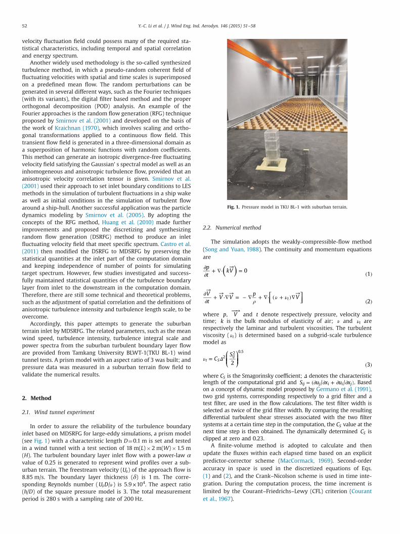
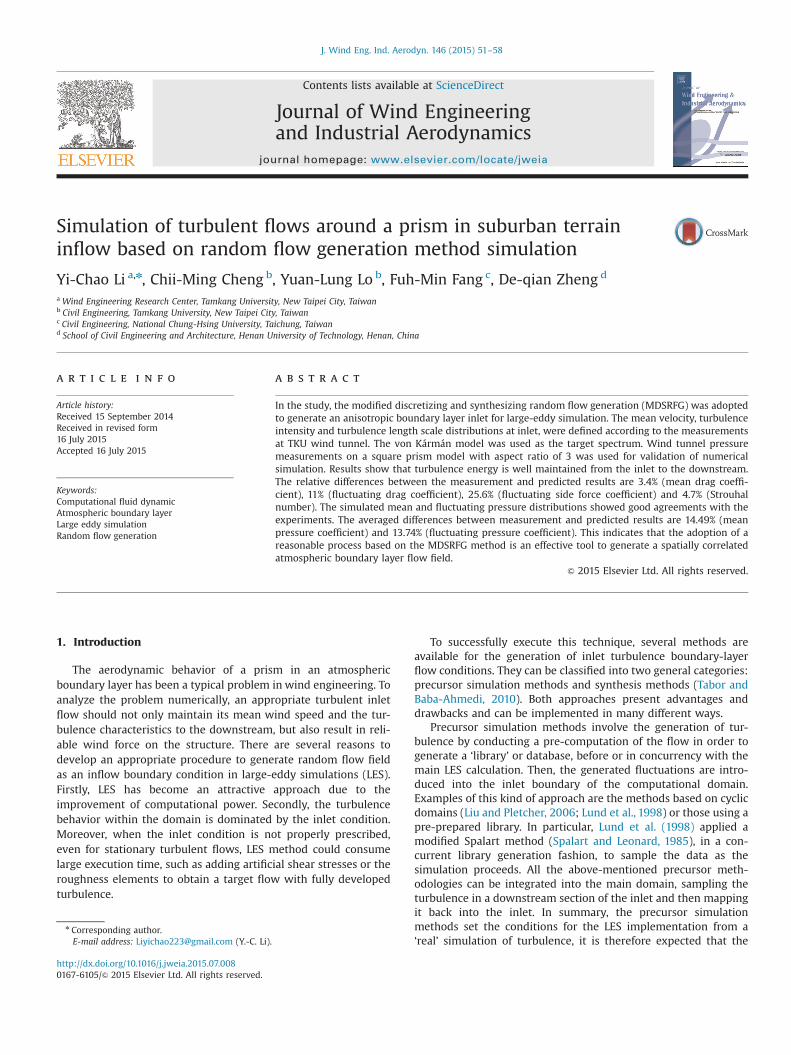
Fig. 1. Pressure model in TKU BL-1 with suburban terrain.

Y.-C. Li et al. / J. Wind Eng. Ind. Aerodyn. 146 (2015) 51–5852

velocity fluctuation field could possess many of the required sta-tistical characteristics, including temporal and spatial correlationand energy spectrum.

Another widely used methodology is the so-called synthesizedturbulence method, in which a pseudo-random coherent field offluctuating velocities with spatial and time scales is superimposedon a predefined mean flow. The random perturbations can begenerated in several different ways, such as the Fourier techniques(with its variants), the digital filter based method and the properorthogonal decomposition (POD) analysis. An example of theFourier approaches is the random flow generation (RFG) techniqueproposed by Smirnov et al. (2001) and developed on the basis ofthe work of Kraichnan (1970), which involves scaling and ortho-gonal transformations applied to a continuous flow field. Thistransient flow field is generated in a three-dimensional domain asa superposition of harmonic functions with random coefficients.This method can generate an isotropic divergence-free fluctuatingvelocity field satisfying the Gaussian' s spectral model as well as aninhomogeneous and anisotropic turbulence flow, provided that ananisotropic velocity correlation tensor is given. Smirnov et al.(2001) used their approach to set inlet boundary conditions to LESmethods in the simulation of turbulent fluctuations in a ship wakeas well as initial conditions in the simulation of turbulent flowaround a ship-hull. Another successful application was the particledynamics modeling by Smirnov et al. (2005). By adopting theconcepts of the RFG method, Huang et al. (2010) made furtherimprovements and proposed the discretizing and synthesizingrandom flow generation (DSRFG) method to produce an inletfluctuating velocity field that meet specific spectrum. Castro et al.(2011) then modified the DSRFG to MDSRFG by preserving thestatistical quantities at the inlet part of the computation domainand keeping independence of number of points for simulatingtarget spectrum. However, few studies investigated and success-fully maintained statistical quantities of the turbulence boundarylayer from inlet to the downstream in the computation domain.Therefore, there are still some technical and theoretical problems,such as the adjustment of spatial correlation and the definitions ofanisotropic turbulence intensity and turbulence length scale, to beovercome.

Accordingly, this paper attempts to generate the suburbanterrain inlet by MDSRFG. The related parameters, such as the meanwind speed, turbulence intensity, turbulence integral scale andpower spectra from the suburban turbulent boundary layer floware provided from Tamkang University BLWT-1(TKU BL-1) windtunnel tests. A prism model with an aspect ratio of 3 was built; andpressure data was measured in a suburban terrain flow field tovalidate the numerical results.

2. Method

2.1. Wind tunnel experiment

In order to assure the reliability of the turbulence boundaryinlet based on MDSRFG for large-eddy simulations, a prism model(see Fig. 1) with a characteristic length D¼0.1 m is set and testedin a wind tunnel with a test section of 18 m(L)�2 m(W)�1.5 m(H). The turbulent boundary layer inlet flow with a power-law αvalue of 0.25 is generated to represent wind profiles over a sub-urban terrain. The freestream velocity (Uδ) of the approach flow is8.85 m/s. The boundary layer thickness (δ) is 1 m. The corre-sponding Reynolds number (U D/νδ ) is 5.9×104. The aspect ratio(h/D) of the square pressure model is 3. The total measurementperiod is 280 s with a sampling rate of 200 Hz.

2.2. Numerical method

The simulation adopts the weakly-compressible-flow method(Song and Yuan, 1988). The continuity and momentum equationsare

pt

kV 0 1( )∂∂

+ ∇⋅→

= ( )

⎡⎣⎢

⎤⎦⎥

Vt

V Vp

V2

tρν ν∂

→

∂+

→⋅∇

→= − ∇ + ∇⋅ ( + )∇

→( )

where p, V⎯ →⎯⎯⎯

and t denote respectively pressure, velocity andtime; k is the bulk modulus of elasticity of air; ν and tν arerespectively the laminar and turbulent viscosities. The turbulentviscosity ( tν ) is determined based on a subgrid-scale turbulencemodel as

⎛⎝⎜⎜

⎞⎠⎟⎟C

S

2 3t S

ij22 0.5

ν Δ=( )

where CS is the Smagorinsky coefficient; Δ denotes the characteristiclength of the computational grid and S u x u x/ /ij j i i j= (∂ ∂ + ∂ ∂ ). Basedon a concept of dynamic model proposed by Germano et al. (1991),two grid systems, corresponding respectively to a grid filter and atest filter, are used in the flow calculations. The test filter width isselected as twice of the grid filter width. By comparing the resultingdifferential turbulent shear stresses associated with the two filtersystems at a certain time step in the computation, the CS value at thenext time step is then obtained. The dynamically determined CS isclipped at zero and 0.23.

A finite-volume method is adopted to calculate and thenupdate the fluxes within each elapsed time based on an explicitpredictor-corrector scheme (MacCormack, 1969). Second-orderaccuracy in space is used in the discretized equations of Eqs.(1) and (2), and the Crank–Nicolson scheme is used in time inte-gration. During the computation process, the time increment islimited by the Courant–Friedrichs–Lewy (CFL) criterion (Courantet al., 1967).

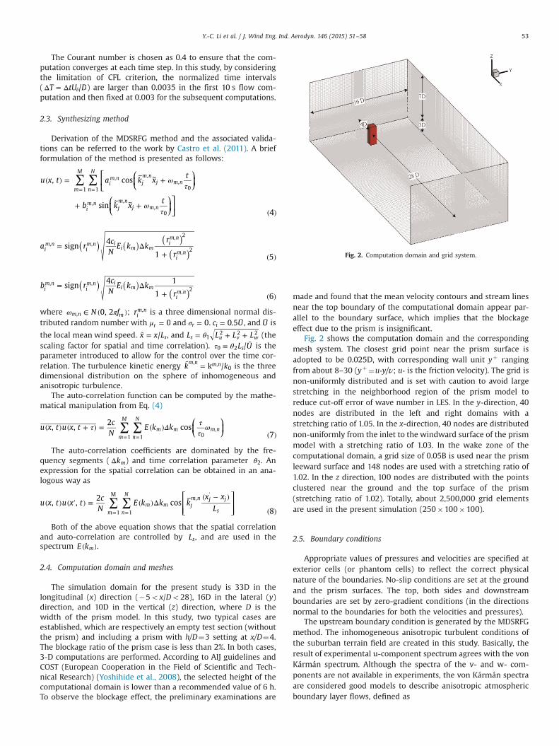
Fig. 2. Computation domain and grid system.

Y.-C. Li et al. / J. Wind Eng. Ind. Aerodyn. 146 (2015) 51–58 53

The Courant number is chosen as 0.4 to ensure that the com-putation converges at each time step. In this study, by consideringthe limitation of CFL criterion, the normalized time intervals( T tU D/Δ = Δ δ ) are larger than 0.0035 in the first 10 s flow com-putation and then fixed at 0.003 for the subsequent computations.

2.3. Synthesizing method

Derivation of the MDSRFG method and the associated valida-tions can be referred to the work by Castro et al. (2011). A briefformulation of the method is presented as follows:

⎡⎣⎢

⎛⎝⎜

⎞⎠⎟

⎛⎝⎜

⎞⎠⎟

⎤⎦⎥

u x t a k xt

b k xt

, cos

sin4

m

M

n

N

im n

jm n

j m n

im n

jm n

j m n

1 1

, ,,

0

, ,,

0

∑ ∑ ωτ

ωτ

( ) =~ ~ +

+~ ~ +

( )

= =

a rc

NE k k

r

rsign

4

1 5im n

im n i

i m mim n

im n

, ,, 2

, 2( ) ( )( )

( )= Δ+ ( )

b rc

NE k k

rsign

4 1

1 6im n

im n i

i m m

im n

, ,

, 2( )( )

( )= Δ+ ( )

where N f0, 2m n m,ω π∈ ( ); rim n, is a three dimensional normal dis-

tributed random number with 0rμ = and 0rσ = . c U0.5i = ¯ , and U is

the local mean wind speed. x x L/ s˜ = , and L L L Ls u v w12 2 2θ= + + (the

scaling factor for spatial and time correlation). L U/s0 2τ θ= ¯ is theparameter introduced to allow for the control over the time cor-relation. The turbulence kinetic energy k kk /m n m n, ,

0˜ = is the three

dimensional distribution on the sphere of inhomogeneous andanisotropic turbulence.

The auto-correlation function can be computed by the mathe-matical manipulation from Eq. (4)

⎛⎝⎜

⎞⎠⎟u x t u x t

cN

E k k, ,2

cos7m

M

n

N

m m m n1 1 0

,∑ ∑τ Δ ττ

ω( ) ( + ) = ( )( )= =

The auto-correlation coefficients are dominated by the fre-quency segments ( kmΔ ) and time correlation parameter 2θ . Anexpression for the spatial correlation can be obtained in an ana-logous way as

⎡⎣⎢⎢

⎤⎦⎥⎥u x t u x t

cN

E k k kx x

L, ,

2cos

8m n

N

m m jm n j j

s1

M

1

,∑ ∑( ) ( ′ ) = ( )Δ~ ( − )

( )= =

′

Both of the above equation shows that the spatial correlationand auto-correlation are controlled by Ls, and are used in thespectrum E km( ).

2.4. Computation domain and meshes

The simulation domain for the present study is 33D in thelongitudinal (x) direction (�5ox/Do28), 16D in the lateral (y)direction, and 10D in the vertical (z) direction, where D is thewidth of the prism model. In this study, two typical cases areestablished, which are respectively an empty test section (withoutthe prism) and including a prism with h/D¼3 setting at x/D¼4.The blockage ratio of the prism case is less than 2%. In both cases,3-D computations are performed. According to AIJ guidelines andCOST (European Cooperation in the Field of Scientific and Tech-nical Research) (Yoshihide et al., 2008), the selected height of thecomputational domain is lower than a recommended value of 6 h.To observe the blockage effect, the preliminary examinations are

made and found that the mean velocity contours and stream linesnear the top boundary of the computational domain appear par-allel to the boundary surface, which implies that the blockageeffect due to the prism is insignificant.

Fig. 2 shows the computation domain and the correspondingmesh system. The closest grid point near the prism surface isadopted to be 0.025D, with corresponding wall unit yþ rangingfrom about 8–30 (yþ¼u*y/ν; u* is the friction velocity). The grid isnon-uniformly distributed and is set with caution to avoid largestretching in the neighborhood region of the prism model toreduce cut-off error of wave number in LES. In the y-direction, 40nodes are distributed in the left and right domains with astretching ratio of 1.05. In the x-direction, 40 nodes are distributednon-uniformly from the inlet to the windward surface of the prismmodel with a stretching ratio of 1.03. In the wake zone of thecomputational domain, a grid size of 0.05B is used near the prismleeward surface and 148 nodes are used with a stretching ratio of1.02. In the z direction, 100 nodes are distributed with the pointsclustered near the ground and the top surface of the prism(stretching ratio of 1.02). Totally, about 2,500,000 grid elementsare used in the present simulation (250�100�100).

2.5. Boundary conditions

Appropriate values of pressures and velocities are specified atexterior cells (or phantom cells) to reflect the correct physicalnature of the boundaries. No-slip conditions are set at the groundand the prism surfaces. The top, both sides and downstreamboundaries are set by zero-gradient conditions (in the directionsnormal to the boundaries for both the velocities and pressures).

The upstream boundary condition is generated by the MDSRFGmethod. The inhomogeneous anisotropic turbulent conditions ofthe suburban terrain field are created in this study. Basically, theresult of experimental u-component spectrum agrees with the vonKármán spectrum. Although the spectra of the v- and w- com-ponents are not available in experiments, the von Kármán spectraare considered good models to describe anisotropic atmosphericboundary layer flows, defined as

Y.-C. Li et al. / J. Wind Eng. Ind. Aerodyn. 146 (2015) 51–5854

⎡⎣⎢

⎤⎦⎥

t S fI U L U

fL Uu componen :

4 /

1 70.8 / 9

uu u

u

2

2 5/6

( ) ( )( )

− ( ) =¯ ¯

+ ¯( )

z/

0 0.25 0.5 0.75 1 1.25 1.50

0.2

0.4

0.6

0.8

1

Experimential=0.25

u/U0 Turbulence

z/

0 0.1 00

0.2

0.4

0.6

0.8

1

α

_

δ δ

Fig. 3. Vertical profiles of inlet condition (a) mean wind spee

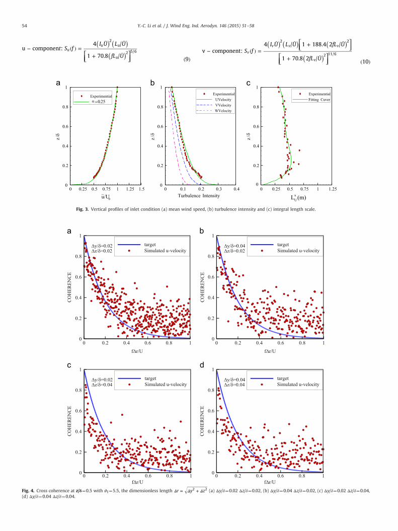
Fig. 4. Cross coherence at z/δ¼0.5 with 1θ ¼5.5, the dimensionless length r y2Δ Δ= +(d) Δy/δ¼0.04 Δz/δ¼0.04.

⎡⎣⎢

⎤⎦⎥

⎡⎣⎢

⎤⎦⎥

S fI U L U fL U

fL Uv component:

4 / 1 188.4 2 /

1 70.8 2 / 10

v

v v v

v

2 2

2 11/6

( ) ( ) ( )( )

− ( ) =¯ ¯ + ¯

+ ¯( )

Intensity.2 0.3 0.4

ExperimentialUVelocityVVelocityWVelocity

LxU(m)

z/

0 0.25 0.5 0.75 1 1.250

0.2

0.4

0.6

0.8

1ExperimentialFitting Cuver

δ

d, (b) turbulence intensity and (c) integral length scale.

z2Δ (a) Δy/δ¼0.02 Δz/δ¼0.02, (b) Δy/δ¼0.04 Δz/δ¼0.02, (c) Δy/δ¼0.02 Δz/δ¼0.04,

Y.-C. Li et al. / J. Wind Eng. Ind. Aerodyn. 146 (2015) 51–58 55

⎡⎣⎢

⎤⎦⎥

⎡⎣⎢

⎤⎦⎥

S f

I U L U fL U

fL U

w component:

4 / 1 188.4 2 /

1 70.8 2 / 11

w

w w w

w

2 2

2 11/6

( ) ( ) ( )( )

− ( )

=¯ ¯ + ¯

+ ¯( )

All the prescribed parameters are obtained from TKU BL1 windtunnel experiments. Regarding the u-component velocity mea-surements, the total measurement period is 60 s with a samplingrate of 500 Hz. The mean wind speed profile is set to follow thepower law with α¼0.25. The longitudinal turbulence intensityprofile is set by I z0.3 0.26 /u

0.35δ= − ( ) . The longitudinal length

Umean/U

z/

0 0.5 10

0.2

0.4

0.6

0.8

1Targetx/D=0x/D=2x/D=4x/D=6x/D=8x/D=10

Iv

z/

0 0.1 0.2 0.3 0.40

0.2

0.4

0.6

0.8

1Targetx/D=0x/D=2x/D=4x/D=6x/D=8x/D=10

δ

δ

δ

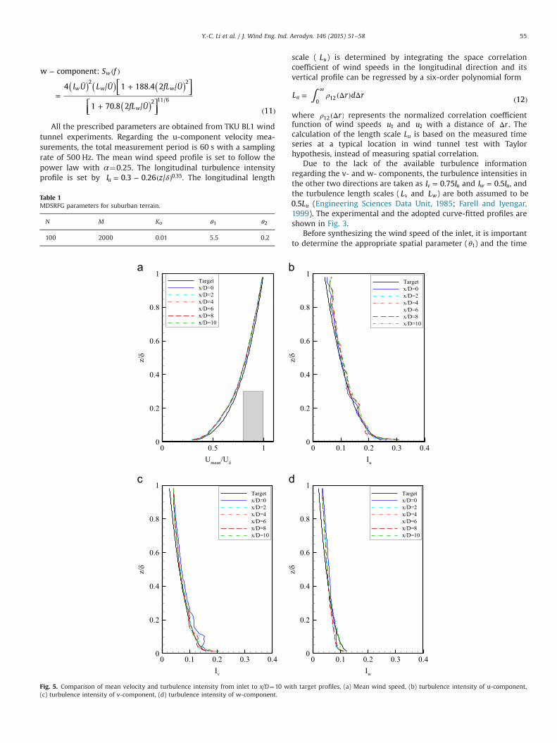
Fig. 5. Comparison of mean velocity and turbulence intensity from inlet to x/D¼10 wi(c) turbulence intensity of v-component, (d) turbulence intensity of w-component.

Table 1MDSRFG parameters for suburban terrain.

N M K0 1θ 2θ

100 2000 0.01 5.5 0.2

scale ( Lu) is determined by integrating the space correlationcoefficient of wind speeds in the longitudinal direction and itsvertical profile can be regressed by a six-order polynomial form

L r d r 12u0

12∫ ρ= (Δ ) Δ ( )∞

where r12ρ (Δ ) represents the normalized correlation coefficientfunction of wind speeds u1 and u2 with a distance of rΔ . Thecalculation of the length scale Lu is based on the measured timeseries at a typical location in wind tunnel test with Taylorhypothesis, instead of measuring spatial correlation.

Due to the lack of the available turbulence informationregarding the v- and w- components, the turbulence intensities inthe other two directions are taken as I I0.75v u= and I I0.5w u= , andthe turbulence length scales ( Lv and Lw) are both assumed to be

L0.5 u (Engineering Sciences Data Unit, 1985; Farell and Iyengar,1999). The experimental and the adopted curve-fitted profiles areshown in Fig. 3.

Before synthesizing the wind speed of the inlet, it is importantto determine the appropriate spatial parameter ( 1θ ) and the time

Iu

z/

0 0.1 0.2 0.3 0.40

0.2

0.4

0.6

0.8

1Targetx/D=0x/D=2x/D=4x/D=6x/D=8x/D=10

Iw

z/

0 0.1 0.2 0.3 0.40

0.2

0.4

0.6

0.8

1Targetx/D=0x/D=2x/D=4x/D=6x/D=8x/D=10

δ

δ

th target profiles. (a) Mean wind speed, (b) turbulence intensity of u-component,

Y.-C. Li et al. / J. Wind Eng. Ind. Aerodyn. 146 (2015) 51–5856

parameter ( 2θ ). 1θ dominates the scaling factor according to thedefinition in Section 2.3, influences the spatial and time correla-tion. Although Eq. (8) gives a convenient way to estimate thespatial correlation between the synthesizing points having thesame form of spectra, the turbulence boundary layer spectra varysignificantly along the vertical direction. In order to define thespatial correlation to determine 1θ , a theoretical equation forreference, the spatial coherence proposed by Davenport (1968), isadopted to be the target function as

⎡⎣ ⎤⎦⎡⎣ ⎤⎦Coh e f

n C z z C y y

U z U z,

0.5 13f z y

21 2

2 21 2

2 1/2

1 2= ^ =

( − ) + ( − )

( ) + ( ) ( )−^

where y1,y2,z1,z2 are the coordinates on the y–z plane. Cy and Cz arethe exponential decay coefficients in the horizontal and verticaldirection respectively. C 10z = and C 16y = are suggested byDavenport (1968) and are consistent with the results of TKU BL1suburban terrain. The experimental coherence function is obtainedfrom calculating the cross spectrum of two simultaneouslyrecorded wind speeds, which is defined as

S r f S r f iS r f, , , 14C Q12 12 12(Δ ) = (Δ ) + (Δ ) ( )

where the real part is known as the co-spectrum and the ima-ginary part is quadrature spectrum. The coherence function is thendefined as

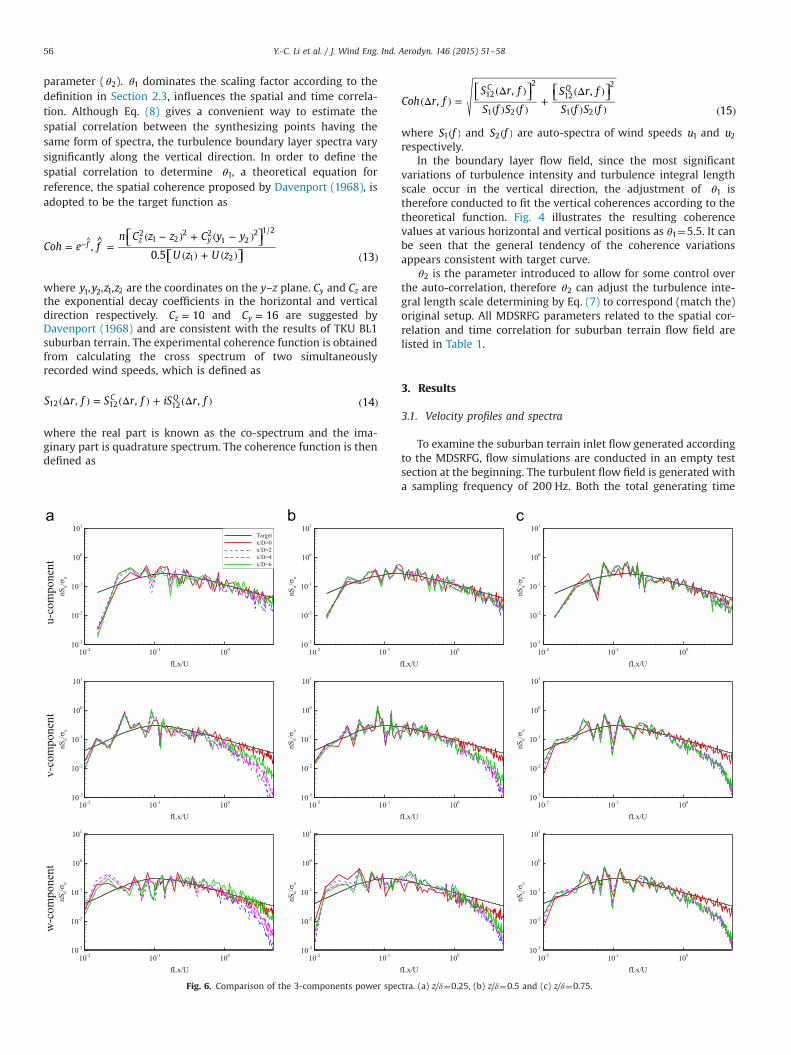
Fig. 6. Comparison of the 3-components power spec

⎡⎣ ⎤⎦ ⎡⎣ ⎤⎦Coh r f

S r f

S f S f

S r f

S f S f,

, ,

15

C Q12

2

1 2

12

2

1 2(Δ ) =

(Δ )

( ) ( )+

(Δ )

( ) ( ) ( )

where S f1( ) and S f2 ( ) are auto-spectra of wind speeds u1 and u2

respectively.In the boundary layer flow field, since the most significant

variations of turbulence intensity and turbulence integral lengthscale occur in the vertical direction, the adjustment of 1θ istherefore conducted to fit the vertical coherences according to thetheoretical function. Fig. 4 illustrates the resulting coherencevalues at various horizontal and vertical positions as 1θ ¼5.5. It canbe seen that the general tendency of the coherence variationsappears consistent with target curve.

2θ is the parameter introduced to allow for some control overthe auto-correlation, therefore 2θ can adjust the turbulence inte-gral length scale determining by Eq. (7) to correspond (match the)original setup. All MDSRFG parameters related to the spatial cor-relation and time correlation for suburban terrain flow field arelisted in Table 1.

3. Results

3.1. Velocity profiles and spectra

To examine the suburban terrain inlet flow generated accordingto the MDSRFG, flow simulations are conducted in an empty testsection at the beginning. The turbulent flow field is generated witha sampling frequency of 200 Hz. Both the total generating time

tra. (a) z/δ¼0.25, (b) z/δ¼0.5 and (c) z/δ¼0.75.

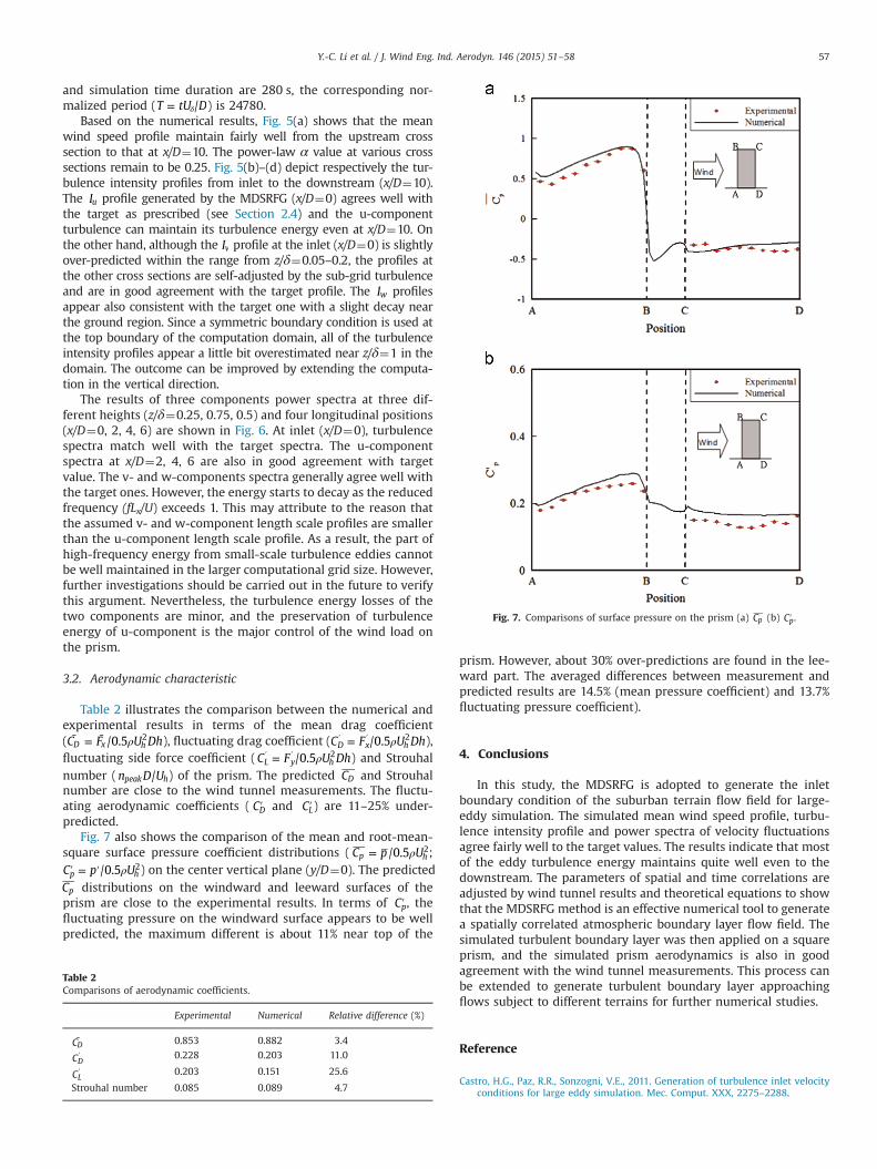
Fig. 7. Comparisons of surface pressure on the prism (a) Cp (b) Cp′ .

Y.-C. Li et al. / J. Wind Eng. Ind. Aerodyn. 146 (2015) 51–58 57

and simulation time duration are 280 s, the corresponding nor-malized period (T tU D/= δ ) is 24780.

Based on the numerical results, Fig. 5(a) shows that the meanwind speed profile maintain fairly well from the upstream crosssection to that at x/D¼10. The power-law α value at various crosssections remain to be 0.25. Fig. 5(b)–(d) depict respectively the tur-bulence intensity profiles from inlet to the downstream (x/D¼10).The Iu profile generated by the MDSRFG (x/D¼0) agrees well withthe target as prescribed (see Section 2.4) and the u-componentturbulence can maintain its turbulence energy even at x/D¼10. Onthe other hand, although the Iv profile at the inlet (x/D¼0) is slightlyover-predicted within the range from z/δ¼0.05–0.2, the profiles atthe other cross sections are self-adjusted by the sub-grid turbulenceand are in good agreement with the target profile. The Iw profilesappear also consistent with the target one with a slight decay nearthe ground region. Since a symmetric boundary condition is used atthe top boundary of the computation domain, all of the turbulenceintensity profiles appear a little bit overestimated near z/δ¼1 in thedomain. The outcome can be improved by extending the computa-tion in the vertical direction.

The results of three components power spectra at three dif-ferent heights (z/δ¼0.25, 0.75, 0.5) and four longitudinal positions(x/D¼0, 2, 4, 6) are shown in Fig. 6. At inlet (x/D¼0), turbulencespectra match well with the target spectra. The u-componentspectra at x/D¼2, 4, 6 are also in good agreement with targetvalue. The v- and w-components spectra generally agree well withthe target ones. However, the energy starts to decay as the reducedfrequency (fLx/U) exceeds 1. This may attribute to the reason thatthe assumed v- and w-component length scale profiles are smallerthan the u-component length scale profile. As a result, the part ofhigh-frequency energy from small-scale turbulence eddies cannotbe well maintained in the larger computational grid size. However,further investigations should be carried out in the future to verifythis argument. Nevertheless, the turbulence energy losses of thetwo components are minor, and the preservation of turbulenceenergy of u-component is the major control of the wind load onthe prism.

3.2. Aerodynamic characteristic

Table 2 illustrates the comparison between the numerical andexperimental results in terms of the mean drag coefficient(C F U Dh/0.5D x h

2ρ¯ = ¯ ), fluctuating drag coefficient (C F U Dh/0.5D x h2ρ=′ ′ ),

fluctuating side force coefficient (C F U Dh/0.5L y h2ρ=′ ′ ) and Strouhal

number (n D U/peak h) of the prism. The predicted CD and Strouhalnumber are close to the wind tunnel measurements. The fluctu-ating aerodynamic coefficients ( CD′ and CL′) are 11–25% under-predicted.

Fig. 7 also shows the comparison of the mean and root-mean-square surface pressure coefficient distributions ( C p U/0.5p h

2ρ= ;C p U/0.5p h

2ρ′ = ′ ) on the center vertical plane (y/D¼0). The predictedCp distributions on the windward and leeward surfaces of theprism are close to the experimental results. In terms of Cp′ , thefluctuating pressure on the windward surface appears to be wellpredicted, the maximum different is about 11% near top of the

Table 2Comparisons of aerodynamic coefficients.

Experimental Numerical Relative difference (%)

CD 0.853 0.882 3.4

CD′ 0.228 0.203 11.0

CL′ 0.203 0.151 25.6

Strouhal number 0.085 0.089 4.7

prism. However, about 30% over-predictions are found in the lee-ward part. The averaged differences between measurement andpredicted results are 14.5% (mean pressure coefficient) and 13.7%fluctuating pressure coefficient).

4. Conclusions

In this study, the MDSRFG is adopted to generate the inletboundary condition of the suburban terrain flow field for large-eddy simulation. The simulated mean wind speed profile, turbu-lence intensity profile and power spectra of velocity fluctuationsagree fairly well to the target values. The results indicate that mostof the eddy turbulence energy maintains quite well even to thedownstream. The parameters of spatial and time correlations areadjusted by wind tunnel results and theoretical equations to showthat the MDSRFG method is an effective numerical tool to generatea spatially correlated atmospheric boundary layer flow field. Thesimulated turbulent boundary layer was then applied on a squareprism, and the simulated prism aerodynamics is also in goodagreement with the wind tunnel measurements. This process canbe extended to generate turbulent boundary layer approachingflows subject to different terrains for further numerical studies.

Reference

Castro, H.G., Paz, R.R., Sonzogni, V.E., 2011. Generation of turbulence inlet velocityconditions for large eddy simulation. Mec. Comput. XXX, 2275–2288.

Y.-C. Li et al. / J. Wind Eng. Ind. Aerodyn. 146 (2015) 51–5858

Courant, R., Friedrichs, K.O., Lewy, H., 1967. On the partial difference equations ofmathematical physics. IBM J. 11, 215–234.

Davenport, A.G., 1968. The dependence of wind load upon Meteorological Para-meter. In: Proceedings of International Research Seminar on Wind Effects onBuildings and Structures. University of Toronto Press, Toronto, pp. 19–82.

Engineering Sciences Data Unit, 1985. Characteristics of Atmospheric TurbulenceNear the Ground. ESDU International Ltd, London, Data Item 85020.

Farell, C., Iyengar, K.S., 1999. Experiments on the wind tunnel simulation ofatmospheric boundary layers. J. Wind Eng. Ind. Aerodyn. 79, 11–35.

Germano, M., Piomelli, U., Moin, P., Cabot, W.H., 1991. A dynamic subgrid-scaleeddy viscosity model. Phys. Fluids 3, 1760–1765.

Huang, S.H., Li, Q.S., Wu, J.R., 2010. A general inflow turbulence generator for largeeddy simulation. J. Wind Eng. Ind. Aerodyn. 98, 600–617.

Kraichnan, R.H., 1970. Diffusion by a random velocity field. Phys. Fluids 13, 22–31.Liu, K.L., Pletcher, R.H., 2006. Inflow conditions for the large eddy simulation of

turbulent boundary layers: a dynamic recycling procedure. J. Comput. Phys. 219(1), 1–6.

Lund, T.S., Wu, X., Squires, K.D., 1998. Generation of turbulent inflow data forspatially-developing boundary layer simulations. J. Comput. Phys. 140,233–258.

MacCormack, R. 1969. The effect of viscosity in hyper-velocity impact cratering.AIAA Paper, pp. 69–354.

Smirnov, A., Celik, I., Shi, S., 2005. Les of bubble dynamics in wake flows. Comput.Fluids 34, 351–373.

Smirnov, R., Shi, S., Celik, I., 2001. Random flow generation technique for large eddysimulations and particle-dynamics modeling. J. Fluids Eng. 123, 359–371.

Song, C., Yuan, M., 1988. A weakly compressible flow model and rapid convergencemethods. J. Fluids Eng. 110 (4), 441–455.

Spalart, P.R., Leonard, A., 1985. Direct numerical simulation of equilibrium turbu-lence boundary layer. In: Proceedings of the 5th Symposium on TurbulentShear Flows. Ithaca, NY.

Tabor, G., Baba-Ahmedi, M., 2010. Inlet conditions for large eddy simulation: areview. Comput. Fluids 39, 553–567.

Yoshihide, T., Akashi, M., Ryuichiro, Y., Hiroto, K., Tsuyoshi, N., Masaru, Y., Taichi, S.,2008. AIJ guidelines for practical applications of CFD to pedestrian windenvironment around buildings. J. Wind Eng. Ind. Aerodyn. 96, 1749–1761.