journal of wind engineering & industrial aerodynamics · local-scale forcing effects on wind...

Journal of Wind Engineering & Industrial Aerodynamics 170 (2017) 238–255

Contents lists available at ScienceDirect

Journal of Wind Engineering & Industrial Aerodynamics

journal homepage: www.elsevier .com/locate/ jweia

Local-scale forcing effects on wind flows in an urban environment: Impact ofgeometrical simplifications

A. Ricci a,b,*, I. Kalkman b, B. Blocken b,c, M. Burlando a, A. Freda a, M.P. Repetto a

a Department of Civil, Chemical and Environmental Engineering (DICCA), University of Genoa, Genoa, Italyb Building Physics and Services, Department of the Built Environment, Eindhoven University of Technology, Eindhoven, The Netherlandsc Building Physics Section, Department of Civil Engineering, KU Leuven, Leuven, Belgium

A R T I C L E I N F O

Keywords:CFD simulationsUrban wind flowModel detailingGeometric uncertaintiesStatistical performance

* Corresponding author. Department of Civil, ChemicalE-mail addresses: [email protected], [email protected]

[email protected] (M. Burlando), [email protected]

http://dx.doi.org/10.1016/j.jweia.2017.08.001Received 14 September 2016; Received in revised form 2

0167-6105/© 2017 The Authors. Published by Elsevier L

A B S T R A C T

Wind flow in urban areas is strongly affected by the urban geometry. In the last decades most of the geometriesused to reproduce urban areas, both in wind-tunnel (WT) tests and Computational Fluid Dynamics (CFD) simu-lations, were simplified compared to reality in order to limit experimental effort and computational costs.However, it is unclear to which extent these geometrical simplifications can affect the reliability of the numericaland experimental results. The goal of this paper is to quantify the deviations caused by geometrical simplifica-tions. The case under study is the district of Livorno city (Italy), called “Quartiere La Venezia”. The 3D steadyReynolds-averaged Navier-Stokes (RANS) simulations are solved, first for a single block of the district, then for thewhole district. The CFD simulations are validated with WT tests at scale 1:300. Comparisons are made of meanwind velocity profiles between WT tests and CFD simulations, and the agreement is quantified using four vali-dation metrics (FB, NMSE, R and FAC1.3). The results show that the most detailed geometry provides improvedperformance, especially for wind direction α ¼ 240� (22% difference in terms of FAC1.3).

1. Introduction

The complex morphology of cities renders the analytical descriptionof wind flow in urban areas very difficult. Analytical wind flow modelsare generally well established over flat open terrain, where the windprofiles mainly depend on the aerodynamic roughness of the surface andon thermal stratification. In contrast, wind flow in urban environments isgoverned by a variety of complex factors, such as the heterogeneousgeometry of buildings, flow impingement, separation and recirculationand local thermal effects.

The region above the buildings, usually defined as the urbanboundary layer (UBL), is influenced by continuously changing surfaceroughness, so that the wind flow never reaches a homogeneous equilib-rium condition. The situation is even more complex within the urbancanopy layer (UCL), where streets give rise to complex canyoning effectsthat are strongly dependent on the canyon orientation with respect to theincoming wind. Many researchers have investigated different aspects ofurban flows (see e.g. reviews by Britter and Hanna, 2003; Fernando,2010; Fernando et al., 2010), but at present the UBL is not yet completelyunderstood althoughWT tests and CFD simulations are frequently used in

and Environmental Engineering (DICl (A. Ricci), [email protected] (I.(A. Freda), [email protected] (M

0 July 2017; Accepted 5 August 201

td. This is an open access article und

urban physics and wind engineering to gain increased understanding.In the last decades, several studies have focused on numerical

modeling of wind flow over random urban-like obstacles (e.g. Xie et al.,2008), uniform and staggered building arrays (e.g. Coceal and Belcher,2004; Xie and Castro, 2006; An et al., 2013; Razak et al., 2013), idealizedurban surfaces (e.g. Cheng and Port�e-Agel, 2015), semi-idealized urbancanopies (e.g. Hertwig et al., 2012) and actual urban environments(Blocken et al., 2012; Janssen et al., 2013; Montazeri et al., 2013; GarcíaS�anchez et al., 2014). Errors and uncertainties can be related to thegeometrical model precision, the approximate form of the governingequations (RANS, LES), the turbulence models, the discretizationschemes and the boundary conditions such as the inflow conditions andthe surface roughness (Franke et al., 2007; Blocken et al., 2007a; Har-greaves and Wright, 2007; Tominaga et al., 2008a, b; Emory et al., 2013;Gorl�e et al., 2015). Carpentieri and Robins (2015) analyzed the impact ofmorphological parameters on wind flow in the UCL. Their results showhow the building height variability, the angles between street canyonorientations and incoming wind and other local geometrical features canstrongly influence the characteristics of the urban flow.

Several authors (Chang and Meroney, 2003; Fernando, 2010; Barlow,

CA), University of Genoa, Genoa, Italy.Kalkman), [email protected], [email protected] (B. Blocken), massimiliano..P. Repetto).

7

er the CC BY license (http://creativecommons.org/licenses/by/4.0/).

mailto:[email protected]









http://crossmark.crossref.org/dialog/?doi=10.1016/j.jweia.2017.08.001&domain=pdf

www.sciencedirect.com/science/journal/01676105

http://www.elsevier.com/locate/jweia

http://dx.doi.org/10.1016/j.jweia.2017.08.001

http://creativecommons.org/licenses/by/4.0/



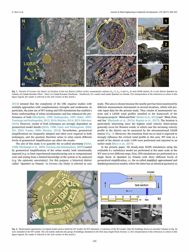
Fig. 1. Pictures of Livorno city (Italy): (a) location of the test district (yellow circle), anemometric stations (Avp 3, Avp 4 and Avp 6) and LiDAR station, (b–c) test district Quartiere LaVenezia, (d) Canale Rosciano (West – East), (e) Canale Rosciano (Northeast – Southwest), (f) a small canal inside Quartiere La Venezia. (For interpretation of the references to colour in thisfigure legend, the reader is referred to the web version of this article.)

A. Ricci et al. Journal of Wind Engineering & Industrial Aerodynamics 170 (2017) 238–255

2013) stressed that the complexity of the UBL requires studies withmultiple approaches with complementary strengths and weaknesses. Inparticular, the joint use of WT testing and CFD simulations has enabled abetter understanding of urban aerodynamics and has enhanced the per-formance of both (Murakami, 1990; Stathopoulos, 1997; Baker, 2007;Tominaga and Stathopoulos, 2013, 2016; Blocken, 2014, 2015; Meroney,2016). However, results of both techniques are strongly dependent ongeometrical model details (AIAA, 1998; Casey and Wintergerste, 2000;AIJ, 2004; Franke, 2006; Blocken, 2014). Nevertheless, geometricalsimplifications are frequently adopted and often even required in bothtechniques, and the question therefore arises to what extent differentlevels of geometrical simplification can affect the results.

The aim of this study is to quantify the so-called uncertainty (AIAA,1998; Oberkampf et al., 2004; Versteeg and Malalasekera, 2007) causedby geometrical simplifications of the urban model, both intentionallyimposed (e.g. to limit experimental manufacturing cost or computationalcost) and arising from a limited knowledge of the system to be analyzed(e.g. the epistemic uncertainty). For this purpose, a historical districtcalled “Quartiere La Venezia” in Livorno city (Italy) is selected as case

Fig. 2. Wind-tunnel experiments: (a) digital model used to build the WT model, (b) WT schemawere included in the WT model. The red outline indicates the group of buildings simulated in tfigure legend, the reader is referred to the web version of this article.)

239

study. This area is chosen because the nearby port has been monitored bydifferent measurement instruments in several locations, which will pro-vide input data for the present study. They consist of anemometric sta-tions and a LiDAR wind profiler installed in the framework of theEuropean projects “Wind and Ports” (Solari et al., 2012) and “Wind, Ports,and Sea” (Burlando et al., 2015a; Repetto et al., 2017). The location isparticularly interesting since the highest wind velocity observationsgenerally occur for Western winds, in which case the incoming velocityprofile in the district can be measured by the aforementioned LiDARstation (Fig. 1). Moreover, the transition from sea to land is expected tostrongly influence the vertical wind profile in this area. WT tests on amodel of the district at scale 1:300 were performed and reported in anearlier study (Ricci et al., 2017).

In the present paper, 3D steady-state RANS simulations using therealizable k-ε turbulence model are performed at the same scale as theWT tests in two different steps. First, CFD simulations are performed on asingle block of Quartiere La Venezia with three different levels ofgeometrical simplification, i.e. the so-called simplified, approximated anddetailed geometrical models, where the latter has an identical geometry as

tic, (c) pictures of the WT model. Only the buildings shown as extruded volumes in Fig. 2ahe first step (single block; Section 3). (For interpretation of the references to colour in this

Fig. 3. Location of measurement positions (a) (L11-14, L21-14, L31-14) and (b) (A11-A52) in the investigated district of Livorno city. The red positions were used for comparison of WT andCFD results (Section 4.2.2). The green positions were only used to compare the results of two CFD models (Section 4.2.2). (For interpretation of the references to colour in this figurelegend, the reader is referred to the web version of this article.)


the WT model. Second, simulations are performed for the whole urbanmodel of Quartiere La Venezia for two of the three levels of geometricalsimplification, i.e. the simplified and the approximated geomet-rical models.

The paper is organized as follows. Section 2 contains a shortdescription of the WT tests used to validate the CFD simulations. Section3 and Section 4 describe two steps of CFD analysis. In particular, Section3 introduces the CFD models (simplified, approximated and detailed), theboundary conditions and the computational setup for the simulations forthe single block of Quartiere La Venezia. On the basis of the obtainedresults, Section 4 describes the CFD simulations for the whole urbandistrict adopting the simplified and approximated models, and shows thecomparison of the WT and CFD results in terms of mean velocity profiles.In Section 5, the level of agreement between WT and CFD results isquantified using validation metrics. Finally, Section 6 (discussion andlimitations) and Section 7 (summary and conclusions) concludethe paper.

2. Description of the wind-tunnel experiments

Only some main aspects of the WT tests are mentioned in this section;the reader is referred to Ricci et al. (2017) for more details. WT tests on ageometrical model of the whole urban district were performed in theatmospheric boundary layer (ABL) wind tunnel of the Department ofCivil, Chemical and Environmental Engineering (DICCA) of the Poly-technic School of the University of Genoa, Italy. The wind tunnel atDICCA is a closed-loop subsonic circuit with a test section of 8.8 m longand a cross-section of 1.70 m (width) x 1.35 m (height) (Fig. 2b). A WTmodel of the case study - Quartiere la Venezia in Livorno city - was createdat a scale of 1:300 using medium density fiberboard (MDF) of differentthicknesses for the ground plates and buildings, and 3 mm closed cellPVC foamboard panels for roofs and bridges (Fig. 2a,c). The blockageratio in the cross-section was kept below 3.5% for all wind directions.

240

Tests were performed for three western wind directions (α ¼ 240�, 270�

and 300�), corresponding to the prevalent wind directions for thestrongest winds in Livorno (Fig. 2a). The mean wind velocity scenariosobtained during the European project “Wind and Ports” (Solari et al.,2012) by means of the WINDS model (Wind Interpolation byNon-Divergent Schemes), anemometric data, and the digital land covermaps of the CORINE project (Bossard et al., 2000) were used as referencefor the choice of the incoming flow profiles in the WT tests. Based on this,an ABL profile with aerodynamic roughness length z0 ¼ 0.1 m (full scale)and friction velocity u* ¼ 0.89 m/s was used for the WT tests.

In the WT tests, the mean wind velocity was measured at two sets ofpositions (Fig. 3). In the first set, 10 positions inside “Canale Rosciano”(A11 - A52) were monitored at 15 heights in the range from 0.02 to 0.6 mabove the wind-tunnel floor (corresponding to 6 m and 180 m full scaleabove mean sea level). Since these positions are fixed to the model ge-ometry, their position in the WT is dependent on model orientation andhence on wind direction. The second set was distributed along a Carte-sian grid laid out according to the WT local reference system, consistingof 15 measurement locations at 15 heights (from 0.02 to 0.6 m above thewind tunnel floor) aligned along three lines of five measurement posi-tions each (L11-5, L21-5, L31-5). Both sets of measurements will be used tovalidate the CFD simulations performed on the urban district, QuartiereLa Venezia, described in Section 4. A third set of measuring positions (L16-14, L26-14, L36-14), indicated in Fig. 3 by the green points, was used toinvestigate the wind velocity profile development in the downstreampart of the computational domain. The results of this investigation aredescribed in Section 4.

3. CFD simulations of a single block of Quartiere La Venezia

3.1. Computational geometry, domain and grid

In the first step, CFD simulations were performed on a single block of

Fig. 4. Relationship between the WT test-section and the CFD computational domain: (a) top view and (b) side view of wind-tunnel test section. Symbols: (W) width and (H) height of theWT and computational domain; (LWT) length of the test section; (L) distance between the position of the measured wind profile and the end boundary; (LCFD) length of the computationaldomain; (15 hmax) distance between the last building of the urban model and the outlet face of the computational domain, where hmax is the maximum building height.

Fig. 5. Geometry and computational grid on building and ground surfaces for (a) simplified, (b) approximated, (c) detailed geometrical models of a block of buildings of Quartiere La Venezia,for the wind direction α ¼ 240�. The selected group of buildings is indicated by a red outline in Fig. 2a. (For interpretation of the references to colour in this figure legend, the reader isreferred to the web version of this article.)


Quartiere La Venezia (indicated by the red outline in Fig. 2a) at the samescale of the WT tests (1:300) and for wind direction α ¼ 240�, in order topreliminarily investigate the deviations caused by three different levelsof geometrical simplification (i.e. called hereafter simplified, approxi-mated and detailed geometrical models). Based on the CFD results ob-tained in this step, the criteria to realize the geometries of the wholeurban district were chosen for the second step. Fig. 4 shows the rela-tionship between the WT test-section and the CFD computationaldomain. The size of the computational domain wasL � W � H ¼ 5.5 � 1.70 � 1.35 m3, where the width (W) and height (H)are coincident with the WT cross-section. The three CFD geometricalmodels and the associated grids were realized using the software Gambit2.4.6. The first one, termed simplified geometrical model, was obtainedrepresenting the single group of buildings as a single bluff body with aheight equal to the arithmetic average height of that building group(Fig. 5a). The second one, termed approximated geometrical model, wasobtained including buildings with their real ground plan and heights, butreplacing pitched roofs with flat ones (Fig. 5b). To this purpose, theheight of every building was calculated as the average between theheights of the peak and the eaves of the pitched roofs. Note that the pitchof the roofs of Quartiere La Venezia are probably less relevant from the

241

aerodynamic point of view, since these are low-sloped roofs with slopesin the range of only about 5�–10�.

The third one, the detailed geometrical model, was perfectly coinci-dent with the WT geometrical model, including the real ground plan andheights of the buildings including pitched roofs (Fig. 5c). Grid generationfor the simplified and approximated geometrical was performed usingthe surface grid generation technique presented by van Hooff andBlocken (2010) in order to achieve a high-level control over the gridlayout. Grid generation for the detailed geometrical model was per-formed only in part using this technique due to the sloped roof geometry.All three grids were constructing adhering to the best guidelines (Frankeet al., 2007; Tominaga et al., 2008a; Blocken, 2015). The local grid res-olution was taken equal or higher than that in previous studies that usedthe same technique and employed certain grid resolutions based ondetailed grid-sensitivity tests (van Hooff and Blocken, 2010; Blockenet al., 2012). The expansion ratio of the grid was kept below 1.2 every-where in the computational domain and at least thirty cells were usedalong every building edge, which is far beyond the minimum number often mentioned in the best practice guidelines (Franke et al., 2007;Tominaga et al., 2008a). In order to avoid convergence problems andmaximize numerical accuracy, only hexahedral and prismatic cells were

Fig. 6. Inlet profiles: mean wind velocity (U), turbulent kinetic energy (k) and turbulence dissipation rate (ε). Also indicated are measured values (black circles). The height of the tallestbuilding (hmax), as indicated by the blue rectangle in the figure, is equal to 0.15 m (corresponding to 45 m full scale). (For interpretation of the references to colour in this figure legend, thereader is referred to the web version of this article.)

Fig. 7. Boundary conditions for the computational domain.


used for the simplified and approximated geometrical models in line withvan Hooff and Blocken (2010); conversely, hexahedral, prismatic andtetrahedral cells were employed in the detailed model because of thepitched roof geometries. The construction of the computational grid ofthe detailed geometrical model was found to be about five times morecomputationally demanding (user time and processing time combined)than the other two geometrical models. The resulting grids counted 5.9million cells for the simplified geometrical model, 8.5 million cells for theapproximated geometrical model, and 11.8 million cells for the detailedgeometrical model.

3.2. Boundary conditions

In order to reproduce the inflow conditions of the WT tests as accu-rately as possible, the inlet face of the computational domain was placedwhere the approach-flow profile was measured in the WT, that isapproximately 1 m upstream of the first building of the urban model(Fig. 4). Hence, the measured vertical mean velocity profile was pre-scribed, and the vertical profiles of the turbulent kinetic energy k(z) andthe turbulence dissipation rate ε(z) were calculated using the equationsbelow (Tominaga et al., 2008a):

kðzÞ ¼ 12

�σ2uðzÞ þ σ2vðzÞ þ σ2wðzÞ

�(1)

εðzÞ ¼ C0:5μ kðzÞ dU

dz(2)

242

For Eq. (1) the velocity standard deviations σu(z), σv(z) and σw(z)measured in the WT tests were employed. In Eq. (2) the constant Cμ is0.09 and a smoothing function was used to remove excessive numericalnoise introduced by the gradient calculation. Since the WT equipmentdoes not allowmeasurements to be made over the entire height of theWTcross-section, mean wind velocity and velocity standard deviations weredirectly measured only from 0 to 0.6 m and from 1.20 to 1.35 m. In thecentral part, between 0.6 and 1.20 m, these quantities were linearlyinterpolated in order to link both measured parts (Fig. 6). Note that theheight of the tallest building is 0.15 m (corresponding to 45 m full scale)and as a result the particular shape of the vertical profiles above 0.6 m isexpected to be of minor to no importance for the resulting flow patternsbelow the 0.15 m threshold.

At the bottom, sides and top of the domain as well as on the buildingand bridge surfaces, the standard wall functions by Launder and Spalding(1974) with roughness modification by Cecebi and Bradshaw (1977)were employed. At the bottom of the computational domain, an equiv-alent sand-grain roughness height ks equal to 0.0013m (0.39m full scale)was imposed. This value was calculated in accordance with Blocken et al.(2007a) as ks ¼ 9.793 z0/Cs, where Cs (the roughness constant) was takenequal to 2.5 in order to comply with the necessary condition yp > ks,where yp is the distance of the centroid of the first cell from the wall. Thesize of the first near-wall cell was chosen in order to obtain dimensionlesswall unit values yþ in the logarithmic layer range, i.e. 30–300 (Blockenet al., 2007a,b). An overview of these boundary conditions is given inFig. 7. At the sides and top of the domain as well as on the building andbridge surfaces, ks was equal to zero. At the outlet of the domain, zerostatic gauge pressure was imposed.

3.3. Solver settings

The CFD simulations were performed using the open-source CFD codeOpenFOAM 2.3.0 with the 3D steady-state Reynolds-Averaged Navier-Stokes (RANS) approach. The realizable k-ε turbulence model wasadopted for closure (Shih et al., 1995). Second-order discretizationschemes were used for the convective and viscous terms of the governingequations. The SIMPLE algorithm was adopted to couple pressure andvelocity fields (Patankar, 1980; Ferziger and Peri�c, 2002). Numericalconvergence was achieved when the residuals showed no discerniblefluctuation and further decrease during the iterative process. All CFDsimulations were performed on a High Performance Computing (HPC)system at DICCA, using a computer node with 32 cores running in par-allel at 1.4 GHz.

Fig. 8. (a) Perspective view of the selected single block of Quartiere La Venezia and nearby surroundings. Contours of amplification factor in horizontal and vertical plane for (b) simplified,(c) approximated and (d) detailed geometrical models, for wind direction α ¼ 240�, made at 0.02 m above sea level (6 m full scale) and in a vertical centerplane of the computational domain(see Fig. 3a).


3.4. CFD results: comparison of results for the three geometrical models

The amplification factor U/Uin,0.02m is defined as the local wind speeddivided by the inlet wind speed at height z ¼ 0.02 m (Uin,0.02m). Theamplification factor U/Uin,0.60m is defined in the same way but with inletwind speed at height z ¼ 0.60 m. Fig. 8 shows contours of the amplifi-cation factor in a horizontal plane at 0.02 m and in the vertical center-plane through L2 (see Fig. 3a). The CFD results for the three geometricalmodels exhibit almost the same wind-flow patterns upstream of thebuilding block, both in terms of horizontal and vertical contours (Fig. 8).In contrast, significant differences are observed for the approximated anddetailed geometrical models, with respect to the simplified one, at thecourtyard and in the wake (Fig. 8c and d). The differences can beinvestigated more in detail by the mean wind velocity profiles at thepositions C1 - C8 (Fig. 9). In Fig. 9, the axes show the ratio U/Uin,0.6m(abscissa) vs. normalized reference height z/zref (ordinate), with refer-ence height zref ¼ 0.60 m. The deviations of the simplified and approxi-mated geometrical models with respect to the detailed geometrical modelare calculated in terms of differences between mean velocity ratios, U/

243

Uin,0.6, i.e. Δsim ¼ Usim/Uin,0.6 – Udet/Uin,0.6 and Δapp ¼ Uapp/Uin,0.6 – Udet/Uin,0.6, at the positions C1 - C8 and for four different levels (0.05, 0.1,0.15 and 0.2 of z/zref) above the bottom of the domain (Table 1).

In general, the CFD results from the three geometrical models showthe same wind velocity values above z/zref ≈ 0.2. In contrast, theapproximated and detailed geometrical models exhibit significant differ-ences with respect to the simplified geometrical model (below z/zref ≈ 0.2)at all positions except for C1 and C2 (upstream of the obstacle).

In the central part of the computational domain, at positions C3, C4and C5, larger differences in terms of mean velocity ratio are found be-tween the three CFDmodels mostly inside the courtyards of the buildings(for the approximated and detailed geometrical models). The approximatedmodel shows small overestimations at positions C3 and C4 below z/zref ≈0.1 with respect to the detailed model (Table 1). Below z/zref ≈ 0.1, thesimplifiedmodel evidently does not provide any velocity values due to theabsence of the courtyards (Fig. 9 and Table 1). At z/zref ¼ 0.15 and at z/zref ¼ 0.2, the Δapp values are smaller than Δsim (Table 1). Approximatelythe same trend of mean velocity ratio observed at positions C3 and C4 isalso found at position C5 at levels 0.15 and 0.2 of z/zref (Table 1).

Fig. 9. Comparison of the vertical mean wind velocity profiles (zref ¼ 0.60 m) above the points C1 - C8 for the inlet direction α ¼ 240�, for the simplified (CFD sim), approximated (CFD app)and detailed (CFD det) geometrical models. The inlet profile (black dashed line) is also shown for comparison.

Table 1Variation in mean velocity ratio between simplified and detailed models (Δsim), and approximated and detailed geometrical models (Δapp) at positions C1 - C8 (see Fig. 8).

z/zref C1 C2 C3 C4

Δsim Δapp Δsim Δapp Δsim Δapp Δsim Δapp

0.05 0 0.001 0.005 0.002 building 0.018 building �0.0170.1 0 0.001 �0.045 0.028 building 0.044 building 0.0330.15 0 0.001 0.015 0.003 0.015 0.001 0.048 0.0140.20 0.001 0.000 0.012 0.002 0.011 0.001 0.005 0.002

z/zref C5 C6 C7 C8

Δsim Δapp Δsim Δapp Δsim Δapp Δsim Δapp

0.05 building building �0.078 0.003 0.177 0.025 0.142 0.0230.1 building building 0.418 �0.052 0.348 0.052 0.158 0.0400.15 0.082 0.027 0.117 0.066 0.060 0.021 0.034 0.0040.20 0.003 �0.001 0.004 �0.005 0.000 �0.009 �0.008 �0.014


In the downstream part of the computational domain, at positions C6,C7 and C8, very substantial discrepancies in mean velocity ratio arefound between the simplified and the other geometrical models (Fig. 9

244

and Table 1). A flattening of the three curves is observed at the positionsC6 and C7 between 0.05 and 0.15 of z/zref, which increases withdecreasing height of the buildings (Fig. 9). As a matter of fact, in the

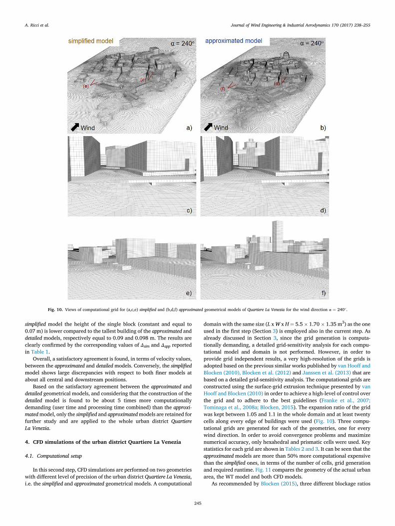
Fig. 10. Views of computational grid for (a,c,e) simplified and (b,d,f) approximated geometrical models of Quartiere La Venezia for the wind direction α ¼ 240� .


simplified model the height of the single block (constant and equal to0.07 m) is lower compared to the tallest building of the approximated anddetailed models, respectively equal to 0.09 and 0.098 m. The results areclearly confirmed by the corresponding values of Δsim and Δapp reportedin Table 1.

Overall, a satisfactory agreement is found, in terms of velocity values,between the approximated and detailed models. Conversely, the simplifiedmodel shows large discrepancies with respect to both finer models atabout all central and downstream positions.

Based on the satisfactory agreement between the approximated anddetailed geometrical models, and considering that the construction of thedetailed model is found to be about 5 times more computationallydemanding (user time and processing time combined) than the approxi-matedmodel, only the simplified and approximatedmodels are retained forfurther study and are applied to the whole urban district QuartiereLa Venezia.

4. CFD simulations of the urban district Quartiere La Venezia

4.1. Computational setup

In this second step, CFD simulations are performed on two geometrieswith different level of precision of the urban district Quartiere La Venezia,i.e. the simplified and approximated geometrical models. A computational

245

domain with the same size (L xW x H¼ 5.5� 1.70� 1.35 m3) as the oneused in the first step (Section 3) is employed also in the current step. Asalready discussed in Section 3, since the grid generation is computa-tionally demanding, a detailed grid-sensitivity analysis for each compu-tational model and domain is not performed. However, in order toprovide grid independent results, a very high-resolution of the grids isadopted based on the previous similar works published by van Hooff andBlocken (2010), Blocken et al. (2012) and Janssen et al. (2013) that arebased on a detailed grid-sensitivity analysis. The computational grids areconstructed using the surface-grid extrusion technique presented by vanHooff and Blocken (2010) in order to achieve a high-level of control overthe grid and to adhere to the best guidelines (Franke et al., 2007;Tominaga et al., 2008a; Blocken, 2015). The expansion ratio of the gridwas kept between 1.05 and 1.1 in the whole domain and at least twentycells along every edge of buildings were used (Fig. 10). Three compu-tational grids are generated for each of the geometries, one for everywind direction. In order to avoid convergence problems and maximizenumerical accuracy, only hexahedral and prismatic cells were used. Keystatistics for each grid are shown in Tables 2 and 3. It can be seen that theapproximated models are more than 50% more computational expensivethan the simplified ones, in terms of the number of cells, grid generationand required runtime. Fig. 11 compares the geometry of the actual urbanarea, the WT model and both CFD models.

As recommended by Blocken (2015), three different blockage ratios

Table 2Comparison of computational grids (in terms of number of cells) for the simplified andapproximated models.

Wind direction Simplified model Approximated model app/sim

α ¼ 240� 13,205,730 23,275,935 1.76α ¼ 270� 11,283,586 20,817,834 1.84α ¼ 300� 11,394,163 19,915,959 1.75

Table 3Comparison of computational time required for the simplified and approximated models.

Computational time Simplifiedmodel

Approximatedmodel

app/sim

total time for grid generation(h)

432 687 1.59

total runtime (h) 234 402 1.72


are calculated: the vertical blockage ratio BRH, the lateral blockage ratio BRLand the (frontal area) blockage ratio BR. Ideally these ratios should bebelow 17% for the first two and 3% for the last one. The values given inEq. (3) below show that this criterion is met for BRH but not for BR andBRL: especially the value for BRL is quite high. However, the projectedfrontal area gives an overly pessimistic estimate of the importance ofblockage effects due to the existence of streets in the model throughwhich air can flow. Furthermore, since all measurement positions and allpositions of interest are located in the central part of the urbanmodel, theeffect of possible artefacts near the edges of the model on observations inthese positions is expected to be limited. Regardless, most important forthe validation study is that the cross-section of the computational domainmatches the WT cross-section, which is the case.

BR ¼ Abuilding

Adomain¼ 3:5% BRH ¼ Hbuilding

Hdomain¼ 5:8% BRL ¼ Lbuilding

Ldomain¼ 58:8%

(3)

Concerning the other computational settings, the same boundaryconditions, inlet conditions, turbulence model, discretization scheme forthe equations, algorithm solver and cluster machine are used as in thefirst step (Section 3).

Fig. 11. Quartiere La Venezia: view from wind direction α ¼ 240�. (a) Photo of the actual urbacomputational grid of the approximated model.

246

4.2. Comparison of wind-tunnel and CFD results

4.2.1. Contours of amplification factorContours of the amplification factor are analyzed in various hori-

zontal and vertical sections at different heights and widths of thecomputational domain. Fig. 12 shows the amplification factors Uin,0.02m,for both CFD models and for three wind directions.

In Fig. 12a–b (α ¼ 240�), Canale Rosciano is almost aligned with theapproach-flow wind direction and, as a result, the wind flow is funneledthrough the canal. Separation and reversal zones are not observed alongthe canal for this wind direction. Inside the canal, the wind velocity in thesimplified model is substantially higher than in the approximated one.

In Fig. 12c–d (α ¼ 270�), the Canale Rosciano is more sheltered fromthe approaching wind compared to α ¼ 240�. The simplifiedmodel showshigher wind velocities in the central part of the domain (to the North ofthe Canale Rosciano) than the approximated one.

In Fig. 12e–f (α¼ 300�), the Canale Rosciano is more perpendicular tothe approach-flow, and it is therefore to a large degree sheltered by theupstream buildings. The approximated model shows higher wind veloc-ities and more extensive leeward zones at the beginning and the end ofthe canal, respectively. Especially for this wind direction, the CFD sim-ulations are found to be quite sensitive to the geometric detailing.Important differences between the two levels of detail employed in thisstudy are found inside the narrow street and canal, as shown in Fig. 13 forthe amplification factor Uin,0.6m.

Fig. 14 shows contours of the amplification factor Uin,0.6m for bothCFD models at the centerline of the computational domain for α ¼ 240�.Despite the fact that model detail can heavily modify the wind-flowpattern inside the urban district, overall, the thickness of the UBLseems similar in both CFDmodels. Indeed, Fig. 14 shows almost the samehorizontal development of stratification for the simplified and approxi-matedmodels, although the maximum height of the buildings is differentfor both models, i.e. about 0.10 m and 0.15 m (32 and 45 m at full scale)respectively. This is useful information in our understanding of thephysical interpretation of displacement height.

4.2.2. Vertical wind profilesTo analyze the streamwise (horizontal) homogeneity of the approach-

flow profiles, an empty domain with the same size as that for the urbanmodel (see Section 4.1) is employed. The profiles at the inlet face and at

n district, (b) photo of the WT model, (c) computational grid of the simplified model, (d)

Fig. 12. Contours of amplification factor: comparison between simplified and approximated geometrical models for wind directions (a, b) α ¼ 240�, (c, d) α ¼ 270� and (e, f) α ¼ 300�-horizontal sections (left) and axonometric view (right) made at 0.02 m above the bottom (6 m above sea level at full scale). Canale Rosciano is indicated by “CR” in the figures.


247

Fig. 13. Contours of amplification factor in vertical centerplane along lines L2 (see Fig. 3a) for the inlet wind direction α ¼ 300�: comparison between simplified and approximated modelfrom (a–b) birdy-eye view, and (c–d) view from Canale Rosciano.

Fig. 14. Contours of amplification factor in vertical centerplane through lines L2 (see Fig. 3a) wind velocity for the inlet wind direction α ¼ 240�: comparison between (a) simplified and (b)approximated models.


the position of the first building of the urban model are compared alongthe lines L2 (centerline of computational domain) and at 0.02 m abovethe bottom, yielding a relative difference of only 0.91% (with an increaseof the velocity), indicating sufficient horizontal inhomogeneity (Blockenet al., 2007a).

Fig. 15 shows dimensionless mean wind velocity profiles obtainedfrom the WT and CFD models for the three wind directions at four lo-cations. The set of measuring positions placed at the central line of theCanale Rosciano (A22-A52) were chosen in order to understand the can-yoning effects inside the urban district (see Fig. 3b).

Overall, above roughly 0.17 m (50 m full-scale equivalent), corre-sponding to z/zref ffi 0.28, the mean velocity profiles are fairly undis-turbed for all models (WT, simplified and approximated models) andapproximately coincident with the incoming profiles, especially for thewind direction α¼ 240�. For α¼ 240�, the wind is approximately alignedwith the entrance of Canale Rosciano and can flow between the cityblocks rather freely. It is also evident that, when the orientation of theCanale Rosciano is more inclined with respect to the incoming wind (fromα ¼ 240� to α ¼ 300�), at lower heights, the WT and CFD wind velocityprofiles are strongly modified by the buildings and the different degreesof precision with which they are represented turn out to have a largeeffect on the flow, especially inside the narrow street and canal.

Fig. 15a (α ¼ 240�): at position A22, where the incoming flow is

248

aligned with the canal, the agreement between CFD and WT results isquite satisfactory. At position A32 the CFD model predictions are lessaccurate. Intentionally chosen, this position is located directly leeward ofthe important bridge near the city center and in the middle of a cross-roads. At position A42 the level of detail of the CFD model plays a keyrole. In this part of the canal the incoming flow is no longer perfectlyaligned with it, and the wake effects due to the presence of the buildingscan be extremely dependent on their shape. Whereas the mean velocityprofile of the approximated model shows a very similar trend comparedwith the WT profile, the simplified model displays a larger gap to the WTresults between 0.11 and 0.28 of z/zref. In the last position A52, which islocated in the middle of a canal curve, the approximated model againleads to a better prediction than the simplified one. Overall, for this winddirection, the approximated model shows better agreement with WT re-sults than the simplified one. This also holds true for the measuring po-sitions that are not reported here.

Fig. 15b (α ¼ 270�): at position A22 the agreement between the CFDmodels and the WT results is very close in the higher part of the domaindown to z/zref ¼ 0.1 (18 m full scale). However, the discrepancy betweenWT and CFD results is substantial close to the ground. At positions A32and A42 important differences are found between 0 and 0.2 z/zref. Aspreviously stated, these positions are located directly leeward of somebuildings (see also Fig. 12c–d), where the results are affected by the

Fig. 15. Comparison of the vertical mean wind velocity profiles (zref ¼ 0.60 m) along the lines A22-A52 for the inlet directions (a) α ¼ 240�, (b) α ¼ 270� and (c) α ¼ 300�, for the simplifiedmodel (CFD sim), approximated model (CFD app), and WT model (WT). The inlet profile (black dashed line) is also shown for comparison.


249

Fig. 16. Comparison of turbulent kinetic energy profiles (zref ¼ 0.60 m) along the line A32 for the inlet directions (a) α ¼ 240�, (b) α ¼ 270�, (c) α ¼ 300� using the simplified model (CFDsim), approximated model (CFD app), and WT model (WT).


underestimation of the turbulent kinetic energy k due to the steady-stateRANS approach here adopted. As an example, Fig. 16 shows the under-estimation of the turbulent kinetic energy for all wind directions at po-sition A32. The quantitative agreement between WT and CFD results isunsatisfactory for this wind direction, although the qualitative windprofile development of the models inside the Canale Rosciano (from po-sition A22 to A52) is somewhat similar. This was probably due to thecanyoning effects along the water canal. The worst agreement betweenthe WT and CFD results occurs at position A22 below z/zref ¼ 0.15, and atpositions A32, A42 and A52 below z/zref ¼ 0.30.

Fig. 15c (α ¼ 300�): the worst performance of the CFD models isobtained for this wind direction. The buildings located at the edge of theCanale Rosciano represent a barrier for the wind flow. Only for positionA22, located windward of the canal, the comparison is satisfactory. Forthe rest of the positions (A32, A42 and A52) the CFD profiles are quitedifferent from the WT ones. The wind flow is not channeled along theCanale Rosciano and canyoning effects occur in the simulations behindthe buildings placed at the edge of the channel (see Fig. 12e–f). Thisaspect explains the trend of the profiles at different positions. The worstagreement between the WT and CFD results is observed at position A22below z/zref ¼ 0.1, and at positions A32, A42 and A52 belowz/zref ¼ 0.40.

Finally, in order to understand the different wind flow patterns pro-duced by two CFD models (i.e. simplified and approximatedmodels) in thedownstream part of the computational domain, mean velocity profiles oftwo CFD models are compared at the 27 positions (L16-14, L26-14, L36-14)already shown in Fig. 3a. The mean velocity profiles monitored along thecenterline of the computational domain (from L26 to L214) and for thethree wind directions considered, are graphically displayed in Fig. 17.The axes show the ratio U/Uin,0,6m (abscissa) vs. normalized referenceheight z/zref (ordinate), with the incoming wind velocity Uin,0,6m

measured at a reference height of zref ¼ 0.6 m as normalization factor.Overall, the two CFD models show, for each wind direction, a

different wind velocity profile development in the downstream part ofthe computational domain, from the last building of the urban district (atabout the position L25 and L26) to the outlet face (Fig. 17). It is worth tonote that, for the simplified model, where the tallest building (about0.10 m) is lower than the equivalent of the approximated model (about0.15 m), the wind velocity profile reaches almost a complete equilibrium

250

condition, i.e. it does not change anymore, in the downwind distance(from the position L26 to the outlet face of the domain). In contrast, forthe approximated model, for which the mismatch of roughness heights islarger than the simplified model, the mean velocity profile needs a largerdownwind distance to reach an equilibrium condition.

4.2.3. Error analysis along vertical linesA comparison between the CFD and WT test results is made along

vertical lines at the positions A21 and A41 (see also Fig. 3b) for 15heights and three wind directions. Normalized mean wind velocities inthe CFD results and WT data are plotted against each other in Fig. 18.The abscissa reports the ratio between the mean wind velocity measuredat height z and the reference mean wind velocity measured at z ¼ 0.6 m(Uref) in the WT tests; the ordinate axis shows the same ratio for the CFDresults. Fig. 18a shows better agreement between the approximatedmodel and the WT model than between the simplified and the WT model.In the latter case the velocity ratio is substantially overestimatedcompared to the WT data. In contrast, the approximated model showssome underestimation of the velocity values close to the ground. For theinlet wind direction α ¼ 270�, shown in Fig. 18b, discrepancies areobserved between the CFD and WT velocity ratios, especially at positionA41 near the ground. This is found for both CFD models, probably dueto the flow reversal zones close to the walls (see Fig. 12c–d). The resultsshown in Fig. 18c are consistent with those for the central line of theCanale Rosciano (Fig. 15c). The large deviations between CFD and WTresults highlighted at position A21 for this inflow direction (α ¼ 300�)can be due to the zone of flow separation present at the entrance of thecanal (see Fig. 12e–f). Underestimation and overestimation of the ve-locity ratios occurs at position A41, in the lower and higher part of theprofiles, respectively. Fig. 18 clearly shows one of the limitations of thisstudy. As a matter of fact, the accuracy that can be achieved is mostlikely limited by the deficiencies of the 3D steady state RANS approach.The use of a more accurate geometry may therefore not lead toimproved predictions within the areas where non-stationary wind-flowpatterns occur. This limitation was already pointed out, for instance, byMurakami (1993), Tominaga et al. (2008b) and Blocken et al. (2016),who discussed this issue for building aerodynamics and by Burlandoet al. (2015b), who discussed this issue using an analogous CFD modelto simulate the flow around a vertical axis wind turbine.

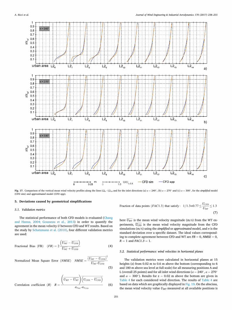
Fig. 17. Comparison of the vertical mean wind velocity profiles along the lines L26 - L214 and for the inlet directions (a) α ¼ 240�, (b) α ¼ 270� and (c) α ¼ 300�, for the simplified model(CFD sim) and approximated model (CFD app).


5. Deviations caused by geometrical simplifications

5.1. Validation metrics

The statistical performance of both CFD models is evaluated (Changand Hanna, 2004; Gousseau et al., 2013) in order to quantify theagreement in the mean velocity U between CFD and WT results. Based onthe study by Schatzmann et al. (2010), four different validation metricsare used:

Fractional Bias ðFBÞ ðFBÞ ¼ 2

�UWT � UCFD

�UWT þ UCFD

(4)

Normalized Mean Square Error ðNMSEÞ NMSE ¼ ðUWT � UCFDÞ2UWT ⋅UCFD

(5)

Correlation coefficient ðRÞ R ¼

UWT � UWT

!�UCFD � UCFD

�σUWT ⋅σUCFD

(6)

251

Fraction of data points ðFAC1:3Þ that satisfy : 1=1:3≈0:77�UCFD

UWT� 1:3

(7)

here UWT is the mean wind velocity magnitude (m/s) from the WT ex-periments, UCFD is the mean wind velocity magnitude from the CFDsimulations (m/s) using the simplified or approximatedmodel, and σ is thestandard deviation over a specific dataset. The ideal values correspond-ing to complete agreement between CFD and WT are FB ¼ 0, NMSE ¼ 0,R ¼ 1 and FAC1.3 ¼ 1.

5.2. Statistical performance: wind velocities in horizontal planes

The validation metrics were calculated in horizontal planes at 15heights (z) from 0.02 m to 0.6 m above the bottom (corresponding to 6and 180 m above sea level at full scale) for all measuring positions A andL (overall 25 points) and for all inlet wind directions (α ¼ 240�, α ¼ 270�

and α ¼ 300�). Results for z ¼ 0.02 m above the bottom are given inTable 4 for each considered wind direction. The results of Table 4 arebased on data which are graphically displayed in Fig. 19. On the abscissa,the mean wind velocity value UWT measured at all available positions is

Fig. 18. Comparison of normalized mean wind velocity values along the vertical profiles A21 and A41 for inlet directions (a) α ¼ 240�, (b) α ¼ 270� and (c) α ¼ 300� for the WT model(WT), simplified and approximated models. Dashed lines correspond to 10% errors.


displayed, normalized with respect to the mean inlet wind velocitymagnitude taken at reference height Uin,0.02 (6 m above sea level at fullscale). The equivalent ratio UCFD/Uin,0.02 of the WT data is reported onthe ordinate.

For a wind direction of α ¼ 240� the FB values of the approximatedmodel clearly shows a tighter distribution around the diagonal comparedto the simplified model, indicating better agreement. For α ¼ 270� thesame FB value is obtained for both CFD models while for α ¼ 300� thesimplified model performed better than the approximated one. A similartrend is observed for the NMSE which shows better performance of theapproximated model for α ¼ 240�. Its performance becomes comparableto that of the simplifiedmodel for α¼ 270� while it is outperformed by thesimplified model for α ¼ 300�. The R of the approximated models is in

252

general quite satisfactory. For α ¼ 240� and α ¼ 300� the approximatedmodel clearly performed better than the simplified model while theyshowed similar performance for α ¼ 270�. Finally, the metric FAC1.3 isused to understand how many data positions fall within 30% of WT data.No difference in the performance of both CFD models is observed in thismetric for α ¼ 270� and α ¼ 300�, while the approximated model per-formed much better for α ¼ 240�.

5.3. Influence of geometrical simplifications on the total drag

In order to assess the effect of the geometrical simplifications on thetotal drag (D), this parameter was calculated for both the simplified andapproximated models (Dsim and Dapp) and for the three wind directions

Table 4Validation metrics (FB ¼ Fractional Bias, NMSE ¼ Normalized Mean Square Error,R ¼ correlation coefficient, FAC1.3 ¼ Fraction of data within a factor of 1.3) for both CFDmodels, three inlet wind directions (α ¼ 240�, α ¼ 270�, α ¼ 300�), and 25 measurementpositions (A and L) at z ¼ 0.02 m above the bottom, corresponding to 6 m above the sealevel at full scale. Also indicated are the number of samples (measurement positions) thatare not occupied by the urban model and are therefore available for statistical analysis(note that this depends on the wind direction as positions L are fixed with respect to the WTsection).

(α ¼ 240�) for z ¼ 0.02 m CFD sim vs WT CFD app vs WT ideal value

FB �0.15 �0.04 0NMSE 0.07 0.04 0R 0.64 0.77 1FAC1.3 0.67 0.89 1samples 18 of 25 18 of 25 25


FB 0.23 0.23 0NMSE 0.13 0.12 0R 0.75 0.76 1FAC1.3 0.50 0.50 1samples 20 of 25 20 of 25 25


FB 0.25 0.30 0NMSE 0.32 0.34 0R 0.35 0.53 1FAC1.3 0.41 0.41 1samples 17 of 25 17 of 25 25

Table 5Comparison of total drag force between simplified and approximated models. The total dragvalues are non-dimensionalized with respect to the total drag force of simplified modelfound for the wind direction α¼ 270�. The ratio in terms of relative difference between twoCFD models is also reported in the last row of the table.

Total drag ratio α ¼ 240� α ¼ 270� α ¼ 300�

Dsim/Dsim,270� 0.84 1.00 1.11Dapp/Dsim,270� 1.01 1.19 1.20Diff. (%) 20.2% 19.0% 8.1%


considered. As expected, for all the CFD cases the most significantcontribution to the total drag is given by the pressure drag associated tothe bluff bodies (i.e. buildings and bridges), whereas the viscous dragcontribution is confined between 2% and 6%, depending on the CFD caseconsidered. In Table 5 the ratio between D and Dsim, 270� (chosen asreference value) is shown for all the CFD models. For all the wind di-rections considered, the drag for the approximated model is higher thanthe simplified one, i.e. þ20.2% for α ¼ 240�, þ19.0% for α ¼ 270� andþ8.1% for α ¼ 300�, as reported in the last row of Table 5, where therelative difference between two CFD models is calculated as ((Dapp/Dsim,270�)-(Dsim/Dsim,270�)/(Dsim/Dsim,270�)). This is possibly attributable tothe higher mean height of the buildings, which yields a higher contri-bution of the pressure drag as well. In addition, the total drag alsochanges according to the wind direction considered.

6. Discussion and limitations

In this case study, the 3D steady-state RANS approach with the real-izable k-ε turbulence model was applied to simulate mean wind-velocitypatterns in a single block of Quartiere La Venezia and in the whole urbandistrict reproduced at reduced scale (1:300). A portion of the WT sectionwas reproduced by the computational domain in order to facilitate thecomparison between WT and CFD results. This study is based on several

Fig. 19. Comparison of CFD and WT data at the monitored positions (A and L) for inlet direc(corresponding to 6 m above sea level at full scale). Dashed black lines correspond to 10% an

253

assumptions:

� The study was performed for only a single city district. Nevertheless,the selected area may be considered representative of many historictowns including different types of buildings and narrow and curvedstreets.

� WT tests and CFD simulations were performed only for a neutrallystratified ABL flow, which typically occurs at the highest windvelocities.

� Three geometries with different degrees of precision were analyzedonly for a single block of Quartiere La Venezia, since the detailedmodelof the whole urban district was found to be extremely computationaldemanding.

� The method used to estimate the height of the buildings (the averagebetween the heights of the peak and eaves of roofs) of the approxi-mated model may be not completely representative of buildings withroofs particularly slanted.

� The CFD simulations were performed using the 3D steady-state RANSapproach, which is known to be deficient especially in separationzones. Large-Eddy Simulation (LES) are currently planned in order toinvestigate the impact of this limitation.

� Only a limited number of measuring positions (25 positions in thehorizontal plane) was taken into account during the WT tests andsubsequently used to validate the CFD results. For each point, how-ever, 15 different heights were monitored, so that the overall numberof points is actually equal to 375. These points, in turn, weremeasured for three wind directions, which means 1125 independentmeasurements.

In spite of these limitations, the CFD simulations of the urban districtshowed a satisfactory agreement with the WT tests for wind directionα ¼ 240� when the finer geometry (approximated model) was used.

7. Summary and conclusions

In this paper the local-scale forcing effects on wind flows in an urbanenvironment were evaluated. In the first step, 3D steady-state RANSsimulations were performed on a single block of a selected case study -

tions: (a) α ¼ 240�, (b) α ¼ 270�, (c) α ¼ 300� at a height z ¼ 0.02 m above the bottomd 30% of errors.


Quartiere la Venezia in Livorno city (Italy) - for one wind direction(α ¼ 240�) and three geometries with different degrees of precision, i.e.simplified, approximated and detailed models. Based on the numerical re-sults found in the first step, a simplified and approximated model of theurban district Quartiere La Venezia were generated and simulated in thesecond step, using the same computational settings employed in the firststep (dimension of domain, boundary conditions, turbulence model, dis-cretization schemes for the equations, algorithm solver). In order toinvestigate to which extent geometrical model details can affect the CFDresults, themeanwind velocity profiles of bothCFDmodels at 25 positionsfor 15 heights each and three different wind directions were comparedwith the WT results. In order to quantify the agreement between the WTand the CFD results, the statistical performance was evaluated using fourdifferent validation metrics: FB, NMSE, R and FAC1.3.

From the first step of this study, the following observations canbe made:

� The simplified model showed large difference in terms of mean ve-locity with respect to the approximated and detailed models, mostly inthe lower part of the wind velocity profiles (Section 3.4).

� The approximated and detailed models showed a satisfactory agree-ment both upstream and downstream of the single block (Section3.4). The small differences in terms of mean velocity found mostly inthe courtyard of the buildings, between two CFD models, do notjustify probably a very high computational effort required to realizeand simulate an eventual detailed model of the entire urban district(Section 3.4).

From the second step of this study, the following observations canbe made:

� The mean velocity contours showed the sensitivity of the simulationsto the different degrees of model precision. The largest differencesbetween the flow fields in the approximated and simplified modelswere found in the narrow streets and canal, especially for the winddirection α ¼ 240� (Section 4.2.1).

� Although the geometric detail can affect the wind-flow pattern insidethe urban district, the thickness of the UBL was similar for both CFDmodels (Section 4.2.1).

� For the wind directions α ¼ 270� and α ¼ 300�, corresponding to adecrease of the flow alignment with respect to the entrance of CanaleRosciano, the agreement between CFD and WT results decreased(Section 4.2.2).

� The CFD results showed an unsatisfactory correspondence betweenthe CFD andWT results in locations where non-stationary phenomenaoccurred. It is likely that here the 3D steady-state RANS approachbecomes the main source of error, in which case a more detailedgeometry will not improve the flow prediction.

� The validation metrics (FB, NMSE, R and FAC1.3) confirmed that thefiner geometry (approximatedmodel) on averageassuresnotablybetterperformance than the coarse one (simplifiedmodel) (Section 5.2).

� The geometrical simplifications applied to the urban model of Quar-tiere La Venezia affected the results also in terms of total drag. Theapproximatedmodel resulted in a higher total drag with respect to thesimplified model for all wind directions considered (Section 5.3).

Overall, wind flowmodeling in urban areas is affected by many errorsand uncertainties related to the inlet conditions, boundary conditions,numerical approach (RANS, LES, DNS), turbulence models, etc. A dis-cussion of all these errors and uncertainties is beyond the scope of thepresent paper, but the future intention is to quantify their relativeimportance for the urban area investigated in this paper. In particular,numerical investigations on the same urban model (at scale 1:300) are inprogress to quantify the uncertainties concerning inlet conditions as wellas the numerical approach (RANS, LES, …).

254

Acknowledgements

The authors gratefully acknowledge the Port Authority of Livorno forthe data of its anemometric monitoring network. All the monitoringdevices and the HPC system at DICCA have been funded by the EuropeanCross-border Programme Italy/France “Maritime” 2007–2013 throughthe “Wind and Port” (CUP: B87E09000000007) and “Wind, Ports, andSea” (CUP: B82F13000100005) projects.

This research has been carried out in the framework of the Project“Wind monitoring, simulation and forecasting for the smart managementand safety of port, urban and territorial systems” funded by “Compagniadi San Paolo” (ID ROL: 9820) in the period 2016–2018.

References

AIAA, 1998. Guide for the Verification and validation of computational fluid dynamicssimulations. AIAA. G-077–1998, ISBN: 1563472856.

An, K., Fung, J.C.H., Yim, S.H.L., 2013. Sensitivity of inflow boundary conditions ondownstream wind and turbulence profiles through building obstacles using a CFDapproach. J. Wind Eng. Ind. Aerodyn. 115, 137–149.

Architectural Institute of Japan, 2004. Recommendations for Loads on Buildings.Architectural Institute of Japan (in Japanese).

Baker, C.J., 2007. Wind engineering – past, present and future. J. Wind Eng. Ind.Aerodyn. 95, 843–870.

Barlow, J.F., 2013. The wind that shakes the buildings: wind engineering from aboundary layer meteorology perspective. In: Owen, J.S., et al. (Eds.), Fifty Years ofWind Engineering: Prestige Lectures from the Sixth European and African Conferenceon Wind Engineering. University of Birmingham.

Blocken, B., 2015. Computational Fluid Dynamics for Urban Physics: importance, scales,possibilities, limitations and ten tips and tricks towards accurate and reliablesimulations. Build. Environ. 91, 219–245.

Blocken, B., 2014. 50 years of computational wind engineering: past, present and future.J. Wind Eng. Ind. Aerodyn. 129, 69–102.

Blocken, B., Janssen, W.D., van Hooff, T., 2012. CFD simulation for pedestrian windcomfort and wind safety in urban areas: general decision framework and case studyfor the Eindhoven University campus. Environ. Model. Softw. 30, 15–34.

Blocken, B., Stathopoulos, T., Carmeliet, J., 2007a. CFD simulation of the atmosphericboundary layer: wall function problems. Atmos. Environ. 41, 238–252.

Blocken, B., Carmeliet, J., Stathopoulos, T., 2007b. CFD evaluation of the wind speedconditions in passages between buildings – effect of wall-function roughnessmodifications on the atmospheric boundary layer flow. J. Wind Eng. Ind. Aerodyn.95, 941–962.

Blocken, B., Stathopoulos, T., van Beeck, J.P.A.J., 2016. Pedestrian-level wind conditionsaround buildings: review of wind-tunnel and CFD techniques and their accuracy forwind comfort assessment. Build. Environ. 100, 50–81.

Bossard, M., Feranec, J., Otahel, J., 2000. Corine Land Cover Technical Guide-addendum2000. Technical Report No 40. EFA, Copenhagen.

Britter, R.E., Hanna, S.R., 2003. Flow and dispersion in urban areas. Annu. Rev. FluidMech. 35, 469–496.

Burlando, M., De Gaetano, P., Pizzo, M., Repetto, M.P., Solari, G., Tizzi, M., Bonino, G.,2015a. The European project wind, ports, and sea. In: Proceedings of the 14thInternational Conference on Wind Engineering, Porto Alegre, Brazil, June 21–26.

Burlando, M., Ricci, A., Freda, A., Repetto, M.P., 2015b. Numerical and experimentalmethods to investigate the behaviour of vertical-axis wind turbines with stators.J. Wind Eng. Ind. Aerodyn. 144, 125–133.

Carpentieri, M., Robins, A.G., 2015. Influence of urban morphology on air flow overbuilding arrays. J. Wind Eng. Ind. Aerodyn. 145, 61–74.

Casey, M., Wintergerste, T., 2000. Best Practice Guidelines, ERCOFTAC Special InterestGroup on Quality and Trust in Industrial CFD. ERCOFTAC, Brussels.

Chang, J.C., Hanna, S.R., 2004. Air quality model performance evaluation. Meteorol.Atmos. Phys. 87, 167–196.

Cebeci, T., Bradshaw, P., 1977. Momentum Transfer in Boundary Layers. HemispherePublishing Corporation, New York.

Chang, C.H., Meroney, R.N., 2003. Concentration and flow distributions in urban streetcanyons: wind tunnel and computational data. J. Wind Eng. Ind. Aerodyn. 91,1141–1154.

Cheng, W.C., Port�e-Agel, F., 2015. Adjustment of turbulent boundary-layer flow toidealized urban surfaces: a large-eddy simulation study. Bound. - Layer. Meteorol.129, 1–23.

Coceal, O., Belcher, S.E., 2004. A canopy model of mean winds through urban areas. Q. J.R. Meteorol. Soc. 130, 1349–1372.

Emory, M., Larsson, J., Iaccarino, G., 2013. Modeling of structural uncertainties inReynolds-averaged Navier-Stokes closures. Phys. Fluids 25, 110822.

Fernando, H.J.S., 2010. Fluid dynamics of urban atmospheres in complex terrain. Annu.Rev. fluid Mech. 42, 365–389.

Fernando, H.J.S., Zajiic, D., Di Sabatino, S., Dimitrova, R., Hedquist, B., Dallman, A.,2010. Flow, turbulence and pollutant dispersion in urban atmospheres. Phys. Fluids22, 051301–1–20.

Ferziger, J.H., Peri�c, M., 2002. Computational Methods for Fluid Dynamics, third ed.Springer-Verlag, ISBN 3-540-42074-6.

Franke, J., Hellsten, A., Schlünzen, H., Carissimo, B., 2007. COST Action 732 QualityAssurance and Improvement of Microscale Meteorological Models.

http://refhub.elsevier.com/S0167-6105(16)30500-1/sref1




























































































Franke, J., 2006. Recommendations of the COST action C14 on the use of CFD inpredicting pedestrian wind environment. In: The Fourth International Symposium onComputational Wind Engineering, Yokohama, Japan, July 2006.

García S�anchez, C., Philips, D.A., Gorl�e, C., 2014. Quantifying inflow uncertainties forCFD simulations of the flow in downtown Oklahoma City. Build. Environ. 78,118–129.

Gorl�e, C., Garcia-Sanchez, C., Iaccarino, G., 2015. Quantifying inflow and RANSturbulence model form uncertainties for wind engineering flows. J. Wind Eng. Ind.Aerodyn. 144, 202–212.

Gousseau, P., Blocken, B., van Heijst, G.J.F., 2013. Quality assessment of Large-EddySimulations of wind flow around a high-rise building: validation and solutionverification. Comput. Fluids 79, 120–133.

Hargreaves, D.M., Wright, N.G., 2007. On the use of the k–ε model in commercial CFDsoftware to model the neutral atmospheric boundary layer. J. Wind Eng. Ind.Aerodyn. 95 (5), 355–369.

Hertwig, D., Efthimiou, G.C., Bartzis, J.G., Leitl, B., 2012. CFD-RANS model validation ofturbulent flow in a semi-idealized urban canopy. J. Wind Eng. Ind. Aerodyn. 111,61–72.

Janssen, W.D., Blocken, B., van Hooff, T., 2013. Pedestrian wind comfort aroundbuildings: comparison of wind comfort criteria based on whole-flow field data for acomplex case study. Build. Environ. 59, 547–562.

Launder, B.E., Spalding, D.B., 1974. The numerical computation of turbulent flows.Comput. Methods Appl. Mech. Eng. 3, 269–289.

Meroney, R.N., 2016. Ten questions concerning hybrid computational/physical modelsimulation of wind flow in the built environment. Build. Environ. 96, 12–21.

Montazeri, H., Blocken, B., Janssen, W.D., van Hooff, T., 2013. CFD evaluation of newsecond-skin facade concept for wind comfort on building balconies: case-study for thePark Tower in Antwerp. Build. Environ. 68, 179–192.

Murakami, S., 1993. Comparison of various turbulence models applied to a bluff body.J. Wind Eng. Ind. Aerodyn. 46–47, 21–36.

Murakami, S., 1990. Computational wind engineering. J. Wind Eng. Ind. Aerodyn. 36,517–538.

Oberkampf, W.L., Trucano, T.G., Hirsch, C., 2004. Verification, validation, and predictivecapability in computational engineering and physics. Appl. Mech. Rev. 57, 345–384.

Patankar, S.V., 1980. Numerical Heat Transfer and Fluid Flow. McGraw-Hill bookcompany, ISBN 0-07-048740-5.

Razak, A.A., Hagishima, A., Ikegaya, N., Tanimoto, J., 2013. Analysis of airflow overbuilding arrays for assessment of urban wind environment. Build. Environ. 59,56–65.

255

Repetto, M.P., Burlando, M., Solari, G., De Gaetano, P., Pizzo, M., Tizzi, M., 2017. A web-based GIS platform for the safe management and risk assessment of complexstructural and infrastructural systems exposed to wind. Adv. Eng. Softw. http://dx.doi.org/10.1016/j.advengsoft.2017.03.002 (in press).

Ricci, A., Burlando, M., Freda, A., Repetto, M.P., 2017. Wind tunnel measurements of theurban boundary layer development over a historical district in Italy. Build. Environ.111, 192–206.

Schatzmann, M., Olesen, H., Franke, J., 2010. COST 732 model evaluation case studies:approach and results. COST Action 732.

Shih, T.H., Liou, W.W., Shabbir, A., Zhu, J., 1995. A new k-ε eddy-viscosity model forhigh Reynolds number turbulent flows e model development and validation. Comput.Fluids 24, 227–238.

Solari, G., Repetto, M.P., Burlando, M., De Gaetano, P., Parodi, M., Pizzo, M., Tizzi, M.,2012. The wind forecast for safety management of port areas. J. Wind Eng. Ind.Aerodyn. 104–106, 266–277.

Stathopoulos, T., 1997. Computational wind engineering: past achievements and futurechallenges. J. Wind Eng. Ind. Aerodyn. 67–68, 509–532.

Tominaga, Y., Mochida, A., Yoshie, R., Kataoka, H., Nozu, T., Yoshikawa, M., et al.,2008a. AIJ guidelines for practical applications of CFD to pedestrian windenvironment around buildings. J. Wind Eng. Ind. Aerodyn. 96, 1749–1761.

Tominaga, Y., Mochida, A., Murakami, S., Sawaki, S., 2008b. Comparison of variousrevised k–εmodels and LES applied to flow around a high-rise building model with 1:1:2 shape placed within the surface boundary layer. J. Wind Eng. Ind. Aerodyn. 96(4), 389–411.

Tominaga, Y., Stathopoulos, T., 2013. CFD simulation of near-field pollutant dispersion inthe urban environment: a review of current modelling techniques. Atmos. Environ.79, 716–730.

Tominaga, Y., Stathopoulos, T., 2016. Ten questions concerning modeling of near-fieldpollutant dispersion in the built environment. Build. Environ. 105, 390–402.

van Hooff, T., Blocken, B., 2010. Coupled urban wind flow and indoor natural ventilationmodelling on a high-resolution grid: a case study for the Amsterdam ArenA stadium.Environ. Model. Softw. 25, 51–65.

Versteeg, H.K., Malalasekera, W., 2007. An Introduction to Computational FluidDynamics, second ed. Pearson Education, ISBN 978-0-13-127498-3.

Xie, Z., Coceal, O., Castro, I.P., 2008. Large-eddy simulation of flows over random urbanlike obstacles. Boundary-Layer Meteorol. 129, 1–23.

Xie, Z., Castro, I.P., 2006. LES and RANS for turbulent flow over arrays of wall-mountedobstacles. Flow. Turbul. Combust. 76, 291–312.


























































http://dx.doi.org/10.1016/j.advengsoft.2017.03.002

http://dx.doi.org/10.1016/j.advengsoft.2017.03.002


















































journal of wind engineering & industrial aerodynamics · local-scale forcing effects on wind...

Documents