journal of xx, vol. x, no. x, month year 1 computing …

JOURNAL OF XX, VOL. X, NO. X, MONTH YEAR 1

Computing the Drivable Area of Autonomous RoadVehicles in Dynamic Road Scenes

Sebastian Sontges and Matthias Althoff

Abstract—This paper presents an algorithm for overapprox-imating the drivable area of road vehicles in the presence oftime-varying obstacles. The drivable area can be used to detectwhether a feasible trajectory exists and in which area onecan limit the search of drivable trajectories. For this purposewe abstract the considered road vehicle by a point mass withbounded velocity and acceleration. Our algorithm calculates thereachable occupancy at discrete time steps. At each time step theset is represented by a union of finitely many sets which are eachthe Cartesian product of two 2-dimensional convex polytopes.We demonstrate our method with three examples: i) a trafficsituation with identical dynamic constraints in x- and y- direction,ii) a highway scenario with different lateral and longitudinalconstraints of the dynamics and iii) a highway scenario withdifferent traffic predictions. The examples demonstrate, that wecan compute the drivable area quickly enough to deploy ourapproach in real vehicles.

Index Terms—Autonomous cars, motion prediction, road ve-hicle safety, reachable set.

I. INTRODUCTION

H IGHLY autonomous cars and advanced driver assistancesystems provide a great opportunity for increasing safety

and comfort in transportation. These systems make decisionsautomatically and choose the driving path themselves withoutrelying on a human driver. However, the decision making andtrajectory generation still pose a major challenge. Usually,the planning yields high-dimensional search problems, whichmust be solved with limited computational resources and hardreal-time constraints. These limitations demand appropriateheuristics to accelerate the search and the need for anytimealgorithms which are able to produce solutions in a timelymanner.

In this work, we present a method for computing anoverapproximation of the set of all possible trajectories ofan automated vehicle. Our method constructs the set of allstates that can be reached by a vehicle considering speed andacceleration bounds while moving in a two-dimensional planewith static and dynamic obstacles.

One basic task of an automated vehicle is the trajectorygeneration from the current position to some goal positionwithout causing any collision. A popular approach to generatetrajectories is to cast the trajectory generation problem into agraph search problem [1]. A set of states in the continuousstate space of the vehicle is selected as nodes of a graph.Trajectories connecting these states are added as edges in the

Sebastian Sontges and Matthias Althoff are with the Department of Com-puter Science, Technische Universitat Munchen, Boltzmannstraße 3, 85748Garching, Germany e-mail: [email protected], [email protected].

Manuscript received ; revised

graph. Depending on the motion model, the trajectories aresolutions to a boundary value problem of open or closed-loop dynamical systems, kinematic models or purely geometriccurves. The nodes can be selected in a random fashion [2](e.g. RRT) or according to an appropriate deterministic scheme[3], [4] (e.g. along the lane). Selecting states and trajectoriestailored towards the specific driving task, the structure in theenvironment and the traffic situation can reduce the size ofthe search graph [5]. A trajectory is found when a path inthe graph is found that connects the initial node to one in thegoal region. One major drawback of graph-based approachesis that the size of the graph scales exponentially with respectto the number of search dimensions. This may quickly lead torestrictive, long search times. Suppose a vehicle can movein a two-dimensional plane with time-dependent obstacles.A vehicle model with two position variables, two velocityvariables and one time variable yields a 5-dimensional searchspace. An exhaustive search for an appropriate, dense selec-tion of trajectories is therefore difficult. An early approachfor reducing complexity involves decomposing the trajectorygeneration to a path planning problem in a static environmentand a velocity planning problem in path-time space [6]. Indynamic scenarios, this decomposition can be too restrictive.A more general approach is to use heuristics to reduce thesearched subspace of the graph [7] and to accept suboptimalsolutions [8]. Besides graph-based approaches, other methodssuch as artificial potential fields [9] and cell decompositions[10] are proposed to generate collision free trajectories forautomated vehicles.

Our method calculates the possible search space underconsideration of static and dynamic obstacles and thus signifi-cantly prunes the search space of the search methods reviewedabove. The dynamic obstacles can be arbitrary, time-varyingoccupied regions. The computed set is an overapproximationof the set of all states which can be reached by the hostvehicle. This set is often referred to as the reachable set. Itis guaranteed that all solution trajectories lie within this set.All trajectories leaving the reachable set during planning canbe proven to either violate the constraints on the dynamicsor eventually collide. A related approach considering setsof reachable states instead of trajectories is presented in[11] which computes the backward reachable set of a goalregion using a method based on the Hamilton-Jacobi-Bellmanequation and involves solving partial differential equations.An approximation of the projected reachable set on a gridin spatial domain using optimal control is introduced in [12].However, it is difficult to include arbitrary shaped time varyingobstacles in this method. In [13] the set of reachable positions


is represented as a time varying polygon but the velocitydomain is neglected.

A second application of our method is to trigger drivingassistant systems, in particular collision mitigation systems.In order to provide the driver with the possibility to avoida collision as long as possible, most collision mitigationsystems only intervene when a collision is no longer avoidable[13], [14]. Many approaches only consider sampled candidatetrajectories, i.e. they check whether no safe solution froma set of finitely many solutions still exists. However, sinceinfinitely many possible trajectories exist, approaches basedon sampling cannot guarantee that a safe trajectory still existsand hence are only resolution or probabilistically complete.However, if our approach returns an empty drivable area,we can prove the non-existence of any evasive maneuver forthe given traffic prediction and can appropriately trigger thecollision mitigation system [15].

A third application of our method is to assess the riskof a traffic situation. Risk assessment has a huge impacton maneuver selection and planning strategies since risk isan essential part for determining optimal trajectories. Anoverview of risk assessment methods can be found in [16].The drivable area of a vehicle as obtained from our work canbe used to deduce risk measures, such as using the area of thedrivable region as a measure to compare alternative plannedtrajectories.

The computation of the drivable area has a lot of re-semblance with classical reachability analysis, but also sig-nificant differences, which require special choices in termsof the applied algorithms and the set representation. Onemain difference is that the computation of the drivable arearequires set difference of the drivable area between the egovehicle and other traffic participants, which results in non-convex and sometimes even non-connected sets. In classicalreachability analysis, however, reachable sets are typicallyrepresented by connected and convex sets, including polytopes[17], zonotopes [18], rectangular grids [19], ellipsoids [20],support functions [21], oriented rectangular hulls [22], andaxis-aligned boxes [23]. We therefore propose a set repre-sentation that borrows ideas from approximative rectangularcell decomposition in the position domain [24] to considerset differences, while we use convex polytopes in the velocitydomain to faithfully consider the vehicle dynamics. A secondmain difference is for the application in road vehicles, theavailable computation time is strictly limited.

The presented algorithm is based on our previous work [15].The novelty of this work is as follows:• Results of preceding and subsequent time steps are used

for the calculations of the reachable set. In our previouswork, the algorithm uses information exclusively fromthe previous step to calculate the next step. In this work,the calculated set is tightened by including informationfrom subsequent steps i.e. excluding states that eventuallyenter forbidden regions.

• The set representation is refined. In our previous work,we approximate the reachable set at each time step by theunion of four-dimensional intervals which may overlap.Here, we approximate the reachable set by an union

of sets, of which each set is the Cartesian product oftwo convex 2-dimensional polytopes. The interior of thesets are disjunct and the boundaries may intersect. Thealgorithmic realization is more efficient despite improvedaccuracy.

• In contrast to our previous work, velocity limits areconsidered. This is particularly important when the cho-sen time horizon is so large, that otherwise meaninglessspeeds are reached.

II. DEFINITIONS AND PROBLEM FORMULATION

A. Reachable set

Given an initial state s0, an input signal u(t) and the systemdynamics s(t) = f(s(t), u(t)), the trajectory of the state is:

s(t) = s0 +

∫ t

t0

f(s(τ), u(τ)) dτ.

We assume a set of forbidden states F(t) to be given. Thereachable set reach(t;X0) is defined as the set of all statesthat can be reached from an initial set X0 at time t:

reach(t;X0) = {s(t;u, s0) |∃u ∈ U , ∃s0 ∈ X0,

s(τ ;u, s0) /∈ F(τ) for τ ∈ [t0, t]}

(1)

where we use the notation s(t;u, s0) to refer to the trajectorywith initial state s0 and input u(t). In the above definition, thereachable set is restricted to states which can only be reachedwithout entering the forbidden states (see Fig. 1).

We additionally define the anticipated reachable set

reachant(t;X0, T ) = {s(t;u, s0) |∃u ∈ U , ∃s0 ∈ X0,

s(τ ;u, s0) /∈ F(τ) for τ ∈ [t0, T ]}

(2)

where t ∈ [t0, T ]. This set is a set of states which can bereached at time t and their trajectories can be continued untiltime T ≥ t without entering the forbidden region (see Fig. 1).It holds that

reachant(t;X0, T ) ⊆ reach(t;X0).

B. Problem statement

We aim at calculating an overapproximation (i.e. a superset)of the anticipated reachable set of a vehicle for a given set ofobstacles which corresponds to a forbidden region F(t). Com-mon vehicle models f(s, u) possess nonlinear behavior andseveral dimensions in the state space, which makes it difficultto calculate the reachable set efficiently. We overapproximatethe vehicle behavior by a moving point mass with boundedacceleration and speed.

The system model used is an abstraction of a realisticvehicle. We motivate this through the following implication:Given a model M of a dynamical system, the model Mi

is an abstraction of M if the reachable set contains theother reachable set, i.e. reachM ⊆ reachMi

. We assumethe acceleration and speed to be bounded, which holds for


t1

t1

t2

t2 T

t1 t2 T

Fig. 1. Reachable set considering collision free trajectories until the given timestep (top). Anticipated reachable set considering only collision free trajectoriesfor the whole planning horizon [t0, T ] (bottom).

all realistic vehicles. Therefore the reachable set of realisticvehicles is a subset of our computed reachable set.

The systems dynamics f(s, u) of the abstract system is:

xxyy

=

0 1 0 00 0 0 00 0 0 10 0 0 0

xxyy

+

0 01 00 00 1

(uxuy)

(3)

|ux| ≤ amax,x|uy| ≤ amax,y

vmin,x ≤ x ≤ vmax,xvmin,y ≤ y ≤ vmax,y

The occupied region of the vehicle in the workspace ismodeled by a disc A(s(t)). We choose the diameter of thedisc to be the diameter of the inner circle of the vehicleshape, since an underapproximation of the shape yields anoverapproximation of the reachable set. The obstacle set O(t)is supposed to be given and defines the forbidden region of theego vehicle. At all times in the planning horizon, the occupiedregion of the vehicle A(s(t)) in the workspace at state s(t)must not intersect with O(t):

∀t : A(s(t)) ∩ O(t) = ∅.

The forbidden region is deduced from the obstacles:

F(t) = {s(t) |A(s(t)) ∩ O(t) 6= ∅} .

In the case of no obstacles, there is a closed-form solutionof the reachable set for our model (3). However, in thepresence of arbitrary obstacles, the set can only be computednumerically since obstacles of arbitrary shape and arrangementinterfere with the closed-form solution. The actual reachableset thus becomes a set that cannot be computed and repre-sented efficiently. The objective of this paper is to presentan algorithm that tightly overapproximates this set, i.e. allapproximations we apply are strict in the sense that the actualreachable set is a subset.

III. MATHEMATICAL MODELING

The dynamics of a state along the x- and y-direction of thesystem (3) is modeled as independent and can be computedseparately. However, to check whether a state lies in theforbidden region F , the pair of positions (x, y) of a state mustbe considered jointly. In this section the mathematical solutionfor the reachable set of the one-dimensional motion along onedirection is shown first. The reachable set of several of theseone-dimensional motions are then merged in our proposedalgorithm shaping an overapproximation of the reachable setof the joined two-dimensional motions.

A. Reachable set of one-dimensional motion

We consider the subproblem of one-dimensional motion in(3), but initially neglect the velocity constraint. In addition, weassume that the system must pass at time t1, t2, . . . , tn someposition interval I1, I2, . . . , In:

(xx

)=

(0 10 0

)︸︷︷︸

A

(xx

)+

(01

)︸︷︷︸B

ux (4)

|ux| ≤ amax,xx(t1) ∈ I1, x(t2) ∈ I2, . . . , x(tn) ∈ In

Suppose the initial states are within a convex initial set X0

at t0 = 0. The reachable set without any position constraint isgiven by

reach(t;X0) ={s

∣∣∣∣∃s0 ∈ X0,∃u ∈ U , s = eAts0 +

∫ t

0

eA(t−τ)Bu(τ)dτ

}= eAtX0 ⊕

{s

∣∣∣∣∃u ∈ U , s =

∫ t

0

eA(t−τ)Bu(τ)dτ

}︸︷︷︸

=:Pu,x(t)

= eAtX0 ⊕ Pu,x (t) (5)

where ⊕ denotes the Minkowski sum, which is defined as:

eAtX0 ⊕ Pu,x (t) ={a+ b

∣∣a ∈ eAtX0, b ∈ Pu,x (t)}.

Pu,x (t) is the set of all states that can be reached froman initial state (x, x)T = (0, 0)T for all possible accelerationconstrained inputs. This region is bounded by the minimumand maximum speeds, that can be reached at each positionafter time t. Given a specific terminal position xt at time t, theminimum/maximum speed at this position can be determinedusing optimal control theory. Pontryagin’s principle yieldsa bang-bang input candidate function with switching timeγt (γ ∈ [0 . . . 1]).

The upper velocity bound (full braking until time γt, thenfull acceleration) is obtained by

x(h)t (γ) = x0 + x0t+ a0t

2

(1

2− 2γ + γ2

)x(h)t (γ) = x0 + amax,xt (1− 2γ)


position [m]

0

2

4

6

8

10ti

me

step

(a)

Position constraints

position [m]−15

−10

−5

0

5

10

15

spee

d[m

/s]

(b)

P1

Pn

Reachable states

−5 0 5

position [m]

−15

−10

−5

0

5

10

15

spee

d[m

/s]

(c)

P1

Pn

Reachable states using backward reach set

Fig. 2. Reachable set of one-dimensional motion of a point mass with boundedacceleration. The position of the point mass is constrained to the intervalsI1 = I2 = · · · = In at time steps 1, 2, . . . , n (a). Forward solution ofthe reachable set (b) and solution using the backward minimal reachable setapproximation (c).

and the lower bound (full acceleration until time γt, then fullbraking) is obtained by

x(l)t (γ) = x0 + x0t− a0t2

(1

2− 2γ + γ2

)x(l)t (γ) = x0 − amax,xt (1− 2γ) .

The upper bound is concave and the lower bound convex.The intersection of both is convex (see Fig. 3).

We calculate the set of possible states Pi at each timestep t1, t2, . . . , tn in a successive manner. First, the set ispropagated one time step further, then it is intersected withthe allowed position interval:

P∗i ⊆(eA(ti−ti−1)Pi−1 ⊕ Pu,x (ti − ti−1)

)∩ (Ii × [−∞,∞]) .

−0.4 −0.2 0.0 0.2 0.4

position [m]

−3

−2

−1

0

1

2

3

speed[m

/s]

x(h)t (γ)

x(l)t (γ)

exact Pu,x

polytope approx. Pu,x

Fig. 3. Closed-form solution Pu,x of the reachable set of an acceleration-bounded point mass with initial state (0, 0)T and a polytope approximationusing supporting halfspaces at switching times γ = 0, 0.5, 1.

If additional speed constraints are considered:

Pi ⊆(eA(ti−ti−1)Pi−1 ⊕ Pu,x (ti − ti−1)

)(6)

∩ (Ii × [vmin,x, vmax,x]) .

The last equation is an overapproximation, since the speedconstraint may be violated in between the time interval.

The set eA(ti−ti−1)Pi−1 ⊕ Pu,x(ti − ti−1) is convex, forconvex Pi−1. However, the curved boundary of Pu,x compli-cates the computation of the Minkowski sum of the sets andthe intersections with halfspaces. To perform these calculationsefficiently, we overapproximate each set by a polytope Pu,xwhich has a fixed number of supporting halfspaces. Each stateon the set boundary corresponds to a switching time of thebang-bang input. The linear equation for one halfspace at someγ is given by (see Fig. 3):

dx(l)t

dγ

dx(l)t

dγ

T∣∣∣∣∣∣∣γ

(0 1−1 0

)T (xtxt

)≤

dx(l)t

dγ

dx(l)t

dγ

T∣∣∣∣∣∣∣γ

(0 1−1 0

)T (x(l)t

x(l)t

)∣∣∣∣∣γ

and similarly for x(h)t . Fig. 2 (b) shows the calculated reach-able sets P1,P2, . . . ,Pn for an example where we choose theintervals I1 = I2 = · · · = In to be equal.

B. Minimal backward reachable set

Considering the same one-dimensional motion (4) from theprevious subsection, some states may propagate over severaltime steps through position intervals but eventually cannotreach an allowed interval in a future time step. Such statesare denoted inevitable collision states (ICS) [25]. The regionof inevitable collision states is determined by the backwardminimal reachable set of the forbidden region [26]. States thatinevitably collide within [0, T ] can contribute to reach(t;X0)


−10−5 0 5 10

position

−10

−5

0

5

10sp

eed

(a)

tj

−10−5 0 5 10

positionsp

eed

(b)

ti

Fig. 4. Position constraint for an acceleration-bounded point mass at time tj(a) and the corresponding allowed states at ti < tj (b).

but do not contribute to reachant(t;X0, T ) and may thereforebe removed during the iterative computation.

The exact computation of ICS yields again a reachabilityanalysis and can therefore in general not be computed effi-ciently [27]. Instead we determine an underapproximative setICS of states which inevitably collide and remove these fromthe iterative computation of reachant:

P ′i := Pi \ ICS = Pi ∩ ICS,

with the complement set (see Appendix A)

ICS(Ij , ti, tj) =

{(xi, xi)

T

∣∣∣∣(−1 −∆tij1 ∆tij

)(xixi

)≤(−Ij,min,x + 1

2amax∆t2ijIj,max,x + 1

2amax∆t2ij

)}.

with ∆tij = tj − ti. Fig. 4 shows the set of feasible states tjfor the constraint x(tj) ∈ Ij . The set ICS(Ij , ti, tj) at tj < ticontains all states which can reach the feasible states at ti.

This can be repeated for all points in time ti < tj ≤ tn tobound the set of all allowed initial states. Thus, the anticipatedreachable set at time ti can be tightened by the constraints afterti:

P ′i := Pi⋂ n⋂

j=i+1

ICS(Ij , ti, tj)

.

P ′i stays convex, since it is an intersection of a convex setwith halfspaces. Fig. 2 (c) shows the tightened reachable setfor the example scenario of the previous section.

IV. ALGORITHM - REACHABLE SET OFTWO-DIMENSIONAL MOTION

So far we have only considered one-dimensional motion.Our proposed algorithm calculates an overapproximation ofthe anticipated reachable set of the two-dimensional motion (3)at discrete points in time. The approximated set is representedas the union Ri of base sets B(q)i , which can be representedefficiently. Each B(q)i is the Cartesian product of two convex2-dimensional polytopes P(q)

i,x/y . Each polytope corresponds toone direction of motion along the x-axis and the y-axis. One

F(ti)

projxy(B(q)i−1)

ti−1

projxy(B(q)i )

propagated

Rect(q)

discretized

Poly(m)

merged

Rect(p)

partitioned

Rect(s)

collision detection and split

(a) (b)

(c) (d)

(e) (f)

Fig. 5. Propagation and overapproximation of the reachable set after one timestep. Shown is the projected reachable set in xy-domain. The reachable set ofthe previous time step (a) is propagated according to the dynamical systemas described in Sec. IV-A. The propagated set (b) is overapproximated (c)-(f)considering collisions with obstacles as described in Sec. IV-B.

axis of each polytope corresponds to the position, the other tospeed:

reachant (ti;X0, T ) ⊆ Ri =⋃q

B(q)i

with B(q)i = P(q)i,x × P

(q)i,y ,

int(B(r)i ) ∩ int(B(l)i ) = ∅ for r 6= l.

(7)

The B(q)i are selected such that the interior is pairwisedisjoint.

The algorithm computes the sets Ri iteratively (see Fig. 5and Alg. 1, ll. 3 - 7; we use the notation {B(q)i }q =

{B(1)i ,B(2)i , . . . } to denote a list of elements). First, the

previous set Ri−1 = ∪qB(q)i−1 is propagated by one timestep according to the dynamical system (6) and ignoring theobstacles O(t). Second, all colliding states are removed fromthe propagated set. The resulting set is overapproximated bya set with representation (7). Third, the new base sets B(q)iare stored as nodes in a graph G. An edge is inserted into Gbetween B(l)i−1 and B(s)i if one is reachable by the other. Eachof these three steps are explained in the following Sec. IV-Ato Sec. IV-C.

A. Flow of the reachable set ignoring obstacles

Both polytopes P(q)i−1,x/y of each B(q)i−1 are propagated

according to the solution of the LTI system with the over-approximation (6) and ignoring any obstacles:

P(q)i,x :=

({(1 ∆t0 1

)s

∣∣∣∣ s ∈ P(q)i−1,x

}⊕ Pu,x(∆t)

)⋂{(

xx

)∣∣∣∣ vmin,x ≤ x ≤ vmax,x}


Algorithm 1

Input: Initial set X0 = ∪qB(q)0 , collision detection for axis-

aligned rectangles with F(t).Output: Graph G with nodes storing {B(q)i }q for i = 1, . . . , n

time steps.

1: function COMPUTEREACHSET(∪qB(q)0 )2: G.INIT(∪qB(q)0 )3: for i = 1 to n do4: ∪qB(q)i ← PROPAGATE(∪qB(q)i−1)5: ∪qB(q)i , E ← OVERAPPROXIMATE(∪qB(q)i \F(ti))6: G.UPDATEGRAPH(∪qB(q)i , E)7: end for8: return G9: end function

10: function PROPAGATE(∪qB(q)i−1)11: for all B(q)i−1 in {B(q)i−1}q do12: P(q)

i,x ← PROPAGATEX(P(q)i−1,x)

13: P(q)i,y ← PROPAGATEY(P(q)

i−1,y)14: B(q)i ← (P(q)

i,x × P(q)i,y )

15: end for16: return ∪B(q)i17: end function

18: function OVERAPPROXIMATE(∪qB(q)i \ F(ti))19: {Rect(·)d } ← DISCRETIZE({projxy(B(·)i )})20: {Poly(·)m } ← MERGE({Rect(·)d })21: {Rect(·)p } ← PARTITION({Poly(·)m })22: {Rect(·)s } ← SPLIT({Rect(·)p })23: E ← OVERLAP({Rect(·)s }, {projxy(B(·)i )})24: for all Rect(l)s in {Rect(l)s }l do25: B(l)i ← CREATEBASESET(Rect(l)s , {B(k)i }(l,k)∈E )26: end for27: return ∪qB(q)i , E28: end function

and similarly for the y-direction (Algorithm 1 Steps 12-13).The propagated set ∪qB(q)i = ∪q(P(q)

i,x ×P(q)i,y ) may intersect

with the set of forbidden states F(ti), and B(q)i may overlapwith each other.

B. Overapproximation of the reachable set considering obsta-cles

In order to consider obstacles and obtain an Ri with the setrepresentation (7) for the next time step, the forbidden statesare removed from ∪qB(q)i and the set is overapproximated suchthat:

Ri = ∪qB(q)i ⊇ (∪qB(q)i \ F(ti)) (8)

where B(q)i are of the form (7).We create this set Ri by partitioning the projection of

∪qB(q)i \ F(ti) in the position domain (see Fig. 5) and assignan overapproximation of the velocity region to each subset ofthe partition.

Fig. 6. Partitioning of an orthogonal polygon into rectangles.

a) Discretize and merge: The merge step computes theunion of the projection of {B(q)i }q in the position domain.The boundaries in the position domain are axis-aligned rect-angles (Algorithm 1 Step 19). We denote these rectangles byRect

(·)d . The union of the rectangles are orthogonal polygons

(Algorithm 1 Step 20). The computation of the polygons isrelated to Klee’s measure problem and can be done efficientlyusing a sweep line algorithm and a segment tree [28]. Ingeneral, the coordinates of the vertices of the polygon arereal numbers. Thus, the calculation would yield orthogonalpolygons with a large number of corners even for slightlydisplaced edges. Therefore we discretize the boundary byenlarging the rectangles to a grid with segment length kg inadvance:

Rect(q)d, min x :=

⌊min(projx(P(q)

i,x ))

kg

⌋· kg

Rect(q)d, max x :=

⌈max(projx(P(q)

i,x ))

kg

⌉· kg

and similarly along the y-direction.b) Partition: The orthogonal polygons of paragraph b)

are split into axis-aligned rectangles (Algorithm 1 Step 21).Through a sweep line algorithm the polygons are cut at eachvertical edge into a rectangle and the remaining polygon. Thiscontinues until the remaining polygon is fully partitioned intorectangles (Fig. 6).

c) Collision detection and splitting: So far, workspaceobstacles have been ignored. In this step (Algorithm 1Step 22), each axis-aligned rectangle is split into two equallysized rectangles if it intersects an obstacle. The split is doneby cutting the axis-aligned rectangle along the middle x- or y-coordinate depending on which one is longer. This is repeateduntil each rectangle is collision free or it collides and itsdiameter is less than the radius of the occupied region of thevehicle A(s(t)) (cf. Sec. II-B). In the latter case, all stateslying in the axis-aligned rectangle intersect an obstacle, andthe states can be excluded. The set of computed Rect(·)s coversthe projection of the desired set (8):

projxy(∪qB(q)i \ F(ti)) ⊆(∪q Rect(q)s

).

d) Overlap: In order to extend the two-dimensional set∪q Rect(q)s of reachable positions to a four-dimensional setwith velocity information, it is determined which Rect

(l)s is

reachable by which B(q)i . The reachable pairs (l, q) are storedin the set E .


B(3)i

B(4)i

B(7)i

B(9)i

B(...)i

B(2)i−1

B(3)i−1

B(4)i−1

B(...)i−1

B(2)i+1

B(5)i+1

B(6)i+1

B(...)i+1

Fig. 7. Relationship between B(q)i of different time steps.

e) Create new base sets: For each Rect(l)s a set B(l)i =

P(l)i,x×P

(l)i,y with an overapproximation of the reachable veloc-

ities is created (Algorithm 1 Step 25). The polytopes P(l)i,x and

P(l)i,y are constructed from the convex hull of the propagated

polytopes of all parent B(k)i intersected with the spatial boundsof the axis-aligned rectangle Rect(l)s :

P(l)i,x =convexhull

⋃(l,k)∈E

(P(k)i,x

⋂{(

xx

)∣∣∣∣Rect(l)s, min x ≤ x ≤ Rect(l)s, max x

})).

The union of the polytopes from the previous time step is ingeneral not convex. We use the convex hull to restore convex-ity. Similarly, the polytope for the y-direction is assigned.

C. Reachability between base sets of succeeding time steps

Usually not all B(·)i−1 can reach all B(·)i in two succeedingtime steps. We express the reachability between sets B(k)i−1 andB(l)i through a graph G (see Fig. 7). Each node in G containsone set B. An edge is added between two nodes if one canreach the other in one time step (l. 6).

V. MULTIPLE RUNS TO REFINE DRIVABLE AREA

In Alg. 1, the reachable set at each time step is constructedfrom the result of the previous time step. This corresponds toan overapproximation of reach(t;X0) (cf. (1)) which neglectsinformation about subsequent steps. For the anticipated reach-able set reachant(t;X0, T ), it is additionally required thatthere is a trajectory which continues each state until time Twithout entering F . This property is difficult to check becauseit leads again to a reachability analysis.

Instead we use two approaches to tighten the overapprox-imation of reachant: i) we remove B(q)i if it does not haveany descendant in G and i is not the last time step (there are

no descendants in the last step) and ii), we calculate addi-tional constraints to apply the simplified concept of inevitablecollision states from Sec. III-B.

The first approach can be readily implemented on the sets{B(q)1 }q, . . . , {B

(q)n−1}q . The second approach is explained in

the following. For each time step we construct an axis-alignedrectangle RectCi in position domain which must be passedby all trajectories. The rectangle constraints RectCi=1,...,n areconstructed by running Alg. 1 once and calculate the boundingbox of {projxy(B(q)i )}q at each time ti. In Sec. III-B it isshown for the one-dimensional case that given a positioninterval, which must be passed at time ti, the set of possibleinitial states at some time t < ti is restricted. We apply thesame technique here. If the state along the x- or y- directioncannot reach either the x- or y- interval of the axis-alignedrectangle of any RectCi in subsequent time steps, it is removed.

The propagation step of Alg. 1 is extended to exclude allthese states:

P(q)i,x =

({(1 ∆t0 1

)s∣∣∣s ∈ P(q)

i−1,x

}⊕ Pu,x(∆t)

)⋂{(

xx

)|vmin,x ≤ x ≤ vmax,x

}⋂ n⋂

j=i

ICS(Ij,x, ti, tj)

where Ij,x denotes the interval of RectCj along the x-axis. Thepropagation along the y-direction is extended similarly.

In some cases a goal region is provided by a high-levelplanner, e.g. an area corresponding to a selected lane at sometime tn = T . The reachant can be used to narrow down theset of initial states which possibly can reach this goal region.After a first run, all B(q)n which intersect the goal region areselected. All of their ancestors up to initial time t0 are selected.For this subset of {B1} , . . . , {Bn} the boundary boxes arecalculated and used as constraints for a second run of thealgorithm as described above.

VI. EXPERIMENTS AND EVALUATION

A. Identical dynamical constraints in x- and y-direction

As a first example we consider the scenario shown in Fig. 8.Two cars A and B are passing each other on two separate lanesin opposite direction. The ego vehicle drives behind car A.

The parameters to compute the drivable area can be chosendepending on the considered application. For emergencysituations high acceleration bounds shall be selected. Lowervalues can be used to compute a bound of a comfortabledrivable area. The following parameters are used for the egovehicle in this examples:

time step ∆t 0.15sabsolute maximum acceleration amax,x/y 10.0 m

s2

minimum speed vmin,x/y −30.0 ms

maximum speed vmax,x/y 30.0 ms

grid size kg 0.5mradius of vehicle 0.9mtime horizon T 3.0s


car B

car Aego car

initial scenario

time: 0.90 sec of 3.00 sec





braking

overtaking

Fig. 8. Drivable area at different time steps in the overtaking scenario.

We suppose that a prediction of car A and car B for thegiven time horizon is provided. In this example, a prediction ofthe occupied region is based on the following assumptions [29]that i) each car stays in the lane and ii) each car may accelerateor brake with 10.0 m

s2 in longitudinal direction, if the speed isbelow some parameterized speed vs. Above vs, acceleration isinversely proportional to speed, up to a maximum speed vmax.We emphasize that the prediction is not part of the presentedalgorithm and is used here only for the sake of the example.Any prediction that provides a collision detection with axis-aligned rectangles at any given point in time can be used incombination with the presented algorithm.

Fig. 8 shows the reachable set at different points in time. Thetwo dark regions are those forbidden due to the prediction ofthe other two cars. The boundary of the street is modeled using

min. speed x-axis

xy

speed

max. speed x-axis

xy

speed

min. speed y-axis

xy

speed

max. speed y-axis

xy

speed

Fig. 9. Boundaries of the reachable velocities at time step 1.5 s of theovertaking scenario.

first run

second run

RectCi constraints from first run

RectCnRectC0

Fig. 10. Refinement of the drivable area of the overtaking maneuver after asecond run of the algorithm.


oriented rectangles (not shown in the figure). The evolutionof the reachable set shows that two maneuvers are implicitlycovered—braking and overtaking. The total number of setsB is 1447. The computation takes approx. 75ms for the 3.0stime horizon in a single-threaded C++ implementation on a2.6 GHz Core i5 (I5-4288U).

The calculated set is 5-dimensional (x, x, y, y, t). Fig. 9shows the covered velocity region at time step 1.5 sec. Tosimplify the plot, only the maximum and minimum speed foreach B in both directions are shown.

In a further step, we select the goal region to be the areaahead of the overtaken car and run the algorithm again for arefinement (cf. Sec. V). Fig. 10 shows the improvement afterthe second run of the algorithm. The region shown for the firstrun are all Bn of the last time step lying in the goal region andall their ancestors. For the second run, the bounding boxes ofeach time step are used to construct constraints. This tightensthe reachable set, particularly in the early time steps. There,a larger number of subsequent constraints apply which shrinkthe area more strongly.

The information gained by the calculated reachable setmight be used for a subsequent trajectory planner. For ex-ample, the narrow passage during overtaking can be easilyidentified. Since any trajectory must lie within the determinedregions, intermediate goal regions at given time steps can beconstructed for a planning algorithm.

B. Different dynamical constraints in lateral and longitudinaldirection

At higher speeds, for example on highways, it is oftenreasonable to consider the lateral and longitudinal directionseparately. On curved roads we choose a coordinate system,which aligns along the center of the road [30]. The longitudinalpositions are located along the arc length of the curved roadcenter, the lateral position is given along the normal vector ofthe road center at a given longitudinal position. This makes itpossible to map a Cartesian coordinate system to the curvedroad. In this example, the reachable set of lateral-longitudinalposition and speeds is determined on a part of a highway asshown in Fig. 11. The cars’ future positions are predicted usingthe assumption that i) each car stays in the lane and ii) eachcar brakes. A safety margin is added behind and in front of allcars. Again, any prediction may be used as long it providescollision checks with axis-aligned rectangles at a given pointin time.

The following parameters are chosen for the ego vehicle inthis examples:

time step ∆t 0.15stime horizon T 3.0sabsolute maximum acceleration (long.) amax,x 10.0 m

s2

minimum speed (long.) vmin,x 0.0 ms

maximum speed (long.) vmax,x 45.0 ms

absolute maximum acceleration (lat.) amax,y 3.0 ms2

minimum speed (lat.) vmin,y −3.0 ms

maximum speed (lat.) vmax,y +3.0 ms

grid size (lat. and long.) kg 0.5mradius of vehicle 0.9m

(a)

(b)

(c)

(d)

(e)

140


(f)

140


(g)

140


(h)

140


(i)

Fig. 11. Reachable set for the same scenario (a) with two different initiallongitudinal speeds of 35 m/s (b) and 43 m/s (d). Underapproximation of thereachable set through a randomly sampled tree of trajectories (c,e-i).


We compare the overapproximation of the reachable setwith a strict underapproximation. The underapproximation iscalculated using a rapidly-exploring random tree [31]. Thestates are connected using an analytical solution for thereachable set of the speed and acceleration bounded system[32]. The exact drivable area of our model is therefore largerthan the one computed by sampling, but smaller than theone computed by our approximative set-based method. Thedistance of the samples to the border of the reachable setindicates the maximum overapproximation.

Two different initial states for the host vehicle are simulated.These two scenarios show the impact of the initial state onthe calculated reachable set. In the first scenario, the initiallongitudinal speed is 35 m/s. In the second scenario, the initiallongitudinal speed is 43 m/s. The initial position and lateralspeed are the same in both cases. The total number of setsB is 1074 and 362, respectively. The computation times are50ms and 20ms. The slower initial speed shows a clearly largerbound of maneuverability region. The reachable set of thefaster initial speed vanishes at prediction time 3.0 sec. Sinceall evasive maneuvers must lie in the reachable set, it provesthat in this case and in the given traffic prediction, no suchmaneuver exists. Possibly, new measures for risk assessmentcan be constructed from properties of the reachable set, forexample its volume or its change of size over different timesteps.

C. Computation with different prediction models

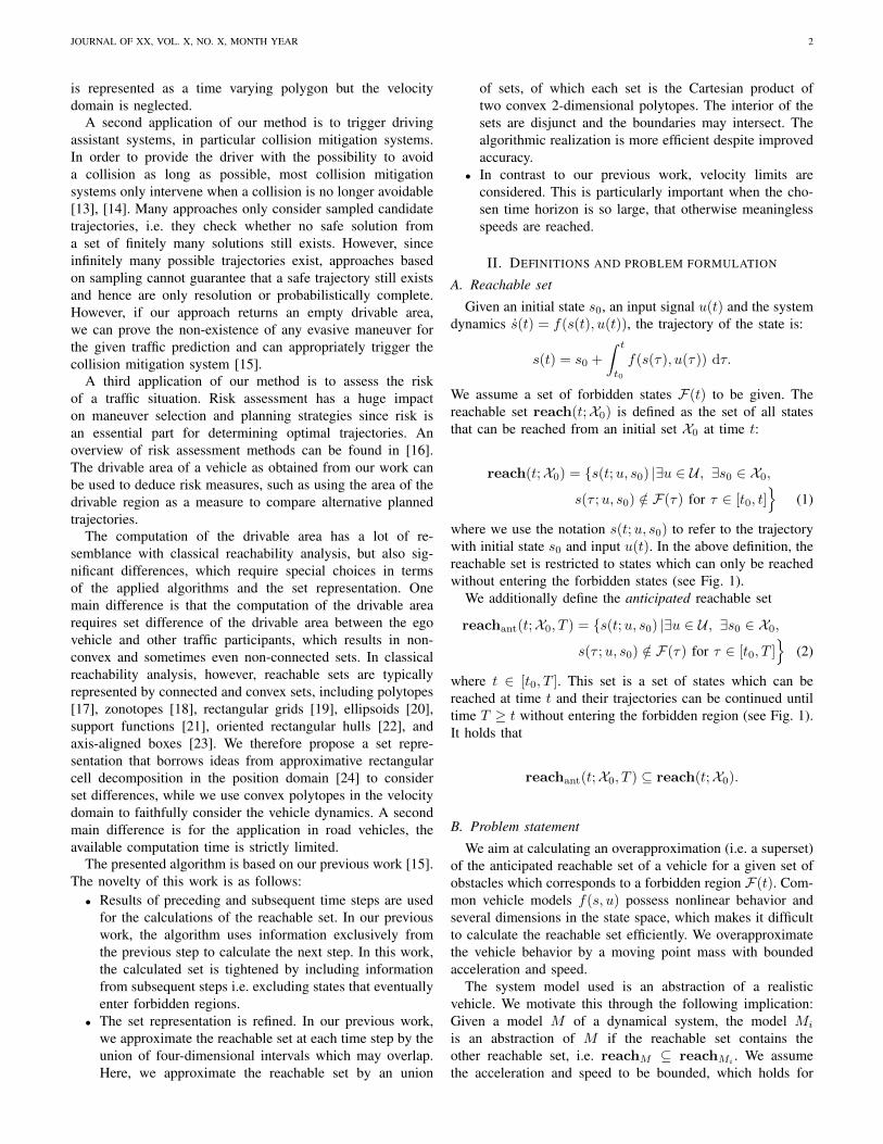
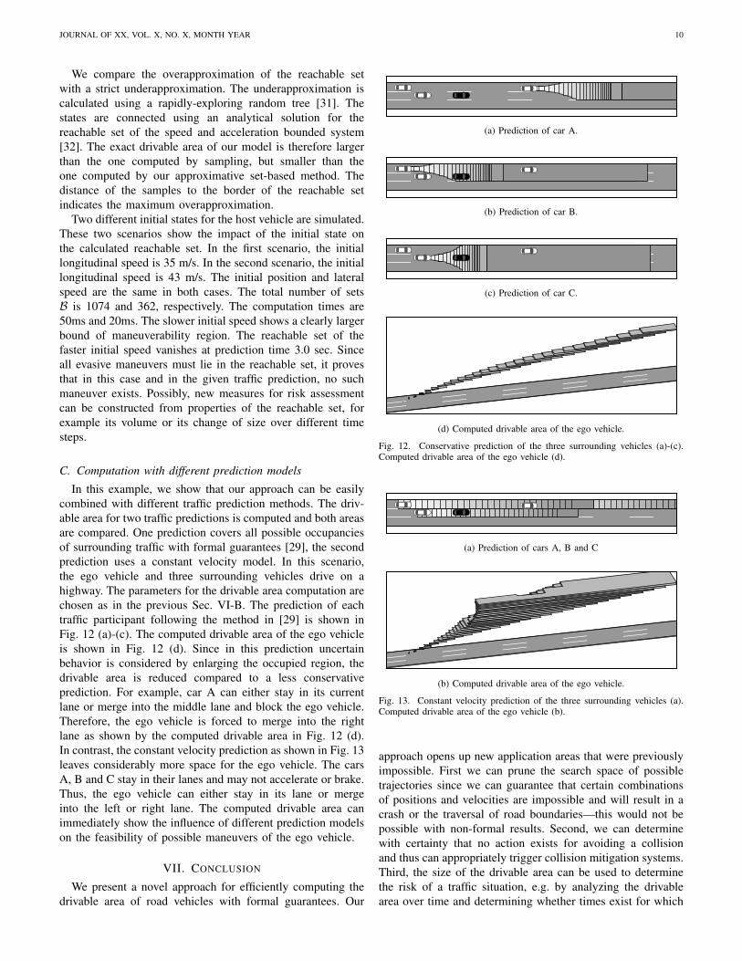
In this example, we show that our approach can be easilycombined with different traffic prediction methods. The driv-able area for two traffic predictions is computed and both areasare compared. One prediction covers all possible occupanciesof surrounding traffic with formal guarantees [29], the secondprediction uses a constant velocity model. In this scenario,the ego vehicle and three surrounding vehicles drive on ahighway. The parameters for the drivable area computation arechosen as in the previous Sec. VI-B. The prediction of eachtraffic participant following the method in [29] is shown inFig. 12 (a)-(c). The computed drivable area of the ego vehicleis shown in Fig. 12 (d). Since in this prediction uncertainbehavior is considered by enlarging the occupied region, thedrivable area is reduced compared to a less conservativeprediction. For example, car A can either stay in its currentlane or merge into the middle lane and block the ego vehicle.Therefore, the ego vehicle is forced to merge into the rightlane as shown by the computed drivable area in Fig. 12 (d).In contrast, the constant velocity prediction as shown in Fig. 13leaves considerably more space for the ego vehicle. The carsA, B and C stay in their lanes and may not accelerate or brake.Thus, the ego vehicle can either stay in its lane or mergeinto the left or right lane. The computed drivable area canimmediately show the influence of different prediction modelson the feasibility of possible maneuvers of the ego vehicle.

VII. CONCLUSION

We present a novel approach for efficiently computing thedrivable area of road vehicles with formal guarantees. Our

(a) Prediction of car A.

(b) Prediction of car B.

(c) Prediction of car C.

(d) Computed drivable area of the ego vehicle.

Fig. 12. Conservative prediction of the three surrounding vehicles (a)-(c).Computed drivable area of the ego vehicle (d).

(a) Prediction of cars A, B and C

(b) Computed drivable area of the ego vehicle.

Fig. 13. Constant velocity prediction of the three surrounding vehicles (a).Computed drivable area of the ego vehicle (b).

approach opens up new application areas that were previouslyimpossible. First we can prune the search space of possibletrajectories since we can guarantee that certain combinationsof positions and velocities are impossible and will result in acrash or the traversal of road boundaries—this would not bepossible with non-formal results. Second, we can determinewith certainty that no action exists for avoiding a collisionand thus can appropriately trigger collision mitigation systems.Third, the size of the drivable area can be used to determinethe risk of a traffic situation, e.g. by analyzing the drivablearea over time and determining whether times exist for which


the solution space is tight, which corresponds to a dangeroussituation. Another possibility to assess the risk of a situationis to compute the drivable area for an uncertain predictionwith probabilistic occupancies with different level sets ofprobability to determine at which level a collision cannot beavoided anymore.

Our method is particularly applicable to problems in dy-namic environments with a short planning horizon of a fewseconds. For these short time horizons, the motion of othervehicles can be predicted reasonably. Our set representationand the construction of our algorithm are tailored towardsan efficient approach despite the necessity to operate in fivedimensions. We have demonstrated in this paper that ourapproach is fast enough to be embedded in automated vehicles.In the future, we plan to exploit the benefits of this approachfor efficient trajectory planning. In particular our approach isable to detect narrow passages between obstacles which areusually difficult to find by trajectory planners.

APPENDIX ADERIVATION OF THE APPROXIMATIVE MINIMAL

BACKWARD REACHABLE SET

Consider the one-dimensional motion with position con-straints (4). We denote the position x at time tj for an initialstate (xi, xi)

T at time ti and an input u(t) by

xj(u;xi, xi) = xi + xi · (tj − ti) +

∫ tj

ti

∫ t

ti

u(τ)dτdt. (9)

If we set the forbidden region to the complement of theposition constraints F(ti) := Ii for t0, . . . , tn, we obtain from(2):

(xi, xi)T ∈ reachant ⇒ ∃u, xj(u;xi, xi) ∈ [Ij,min, Ij,max].

If a state only reaches the forbidden region F for any inputu, it is an ICS and does not belong to reachant:

∀u, xj(u;xi, xi) /∈ [Ij,min, Ij,max]⇒ (xi, xi)T /∈ reachant.

(10)

We denote by ICS an underapproximation of the ICS set.One approximate ICS deduced from (10) is the set of all states(xi, xi) which are accelerated by +amax but their position attj is < Ij,min, and all states which are accelerated by −amaxbut their position at tj is > Ij,max:

ICS(Ij , ti, tj) := {(xi, xi)T | xj(+amax;xi, xi) < Ij,min

∨ xj(−amax;xi, xi) > Ij,max}.(11)

The complement set ICS is obtained from (11) and (9):

ICS(Ij , ti, tj) =

{(xi, xi)

T

∣∣∣∣(−1 −∆tij1 ∆tij

)(xixi

)≤(−Ij,min,x + 1

2amax∆t2ijIj,max,x + 1

2amax∆t2ij

)}with ∆tij = tj − ti.

APPENDIX BCOMPUTATIONAL COMPLEXITY

This section gives a brief summary of the algorithms weuse for the geometric calculations in our implementation. Thenumber of newly created sets Bi in each iteration generallydepends on the obstacle set O(t) and cannot be predicted. Wetherefore give the complexity in terms of b, which denotes themaximum number of elements Bi of all iterations. Similarly,we use the maximum number p of vertices of Pi,x/y in alliterations. The number of time steps is n.

Two polytope representations are distinguished. The V-representation of a polytope through the convex hull of aset of points, and the H-representation through the boundedintersection of a set of halfspaces:Pi,x/y V-representation p pointsPu,x/y V-representation u pointsICS H-representation 2n halfspaces

The points in V-representation are stored either in counter-clockwise order or lexicographically in ascending x-direction.

The complexity of the operations involving convex 2-dimensional polytopes is:

a) Linear mapping eAt Px/y: O(p), result keeps counter-clockwise point order of Px/y for the particular A.

b) Minkowski sum Px/y ⊕ Pu: O(p + u), if both Px/yand Ru are sorted in counter-clockwise order [33, Theorem3.10].

c) Intersection Px/y ∩ (∩nj=0ICS(Ij)): O(p + 2n), if∩nj=0ICS is given in V-representation and both are orderedcounter-clockwise. The conversion from H-representationtakes O(2n log 2n) [33, Corollary 3.10].

d) Convex hull of ∪bq=1P(q)x/y: O(bp log bp) and, if all

points are sorted lexicographically, O(bp) [33, Theorem 1.1].The sorting step can be improved if each P(q)

x/y is ordered

counter-clockwise. The points of each P(q)x/y can be distributed

into two lists: one in lexicographically ascending order, andone in descending order in O(p). Then, all 2n sorted lists aremerged using a k-way merge in O(bp log 2b) [34, Problem9.5-9].

Next, we consider the complexity of the operations in-volving axis-aligned rectangles and orthogonal polygons. Thenumber of edges of polygons is denoted e. For orthogonalpolygons the number of horizontal edges equals the numberof vertical edges ev = e/2.

e) Partition orthogonal polygons into axis-aligned rect-angles: O(ev log ev). We use a sweep line algorithm that cutsparts of the polygon at vertical edges. The active set of verticaledges is kept in an interval tree. It can be shown that thenumber bn of newly created axis-aligned rectangles in thispartition is 2bn ≥ ev ≥ bn. By assumption it holds that b ≥ bn.

f) Merge axis-aligned rectangles to orthogonal polygons:O(b log b+ e log(b2/e)) [28].

g) Overlap between two sets of axis-aligned rectangles:O(b2), if all rectangles of one set overlap with all rectanglesof the other.


ACKNOWLEDGMENT

The authors gratefully acknowledge financial support by theGerman Research Foundation (DFG) AL 1185/3-1

REFERENCES

[1] D. Ferguson, T. M. Howard, and M. Likhachev, “Motion planning inurban environments,” Journal of Field Robotics, vol. 25, no. 11-12, pp.939–960, 2008.

[2] Y. Kuwata, J. Teo, G. Fiore, S. Karaman, E. Frazzoli, and J. P. How,“Real-time motion planning with applications to autonomous urbandriving,” IEEE Transactions on Control Systems Technology, vol. 17,no. 5, pp. 1105–1118, Sep. 2009.

[3] J. Ziegler and C. Stiller, “Spatiotemporal state lattices for fast trajectoryplanning in dynamic on-road driving scenarios,” in IEEE/RSJ Int. Conf.on Intelligent Robots and Systems, 2009, pp. 1879–1884.

[4] M. McNaughton, C. Urmson, J. Dolan, and J.-W. Lee, “Motion planningfor autonomous driving with a conformal spatiotemporal lattice,” inIEEE Int. Conf. on Robotics and Automation, 2011, pp. 4889–4895.

[5] D. Madas, M. Nosratinia, M. Keshavarz, P. Sundstrom, R. Philippsen,A. Eidehall, and K.-M. Dahlen, “On path planning methods for automo-tive collision avoidance,” in IEEE Intelligent Vehicles Symposium, 2013,pp. 931–937.

[6] K. Kant and S. W. Zucker, “Toward efficient trajectory planning: Thepath-velocity decomposition,” The International Journal of RoboticsResearch, vol. 5, no. 3, pp. 72–89, 1986.

[7] D. Dolgov, S. Thrun, M. Montemerlo, and J. Diebel, “Path planning forautonomous vehicles in unknown semi-structured environments,” TheInternational Journal of Robotics Research, vol. 29, no. 5, pp. 485–501, 2010.

[8] M. Likhachev, G. J. Gordon, and S. Thrun, “Ara*: Anytime a* withprovable bounds on sub-optimality,” in Advances in Neural InformationProcessing Systems, 2003, pp. 767–774.

[9] J. Ji, A. Khajepour, W. W. Melek, and Y. Huang, “Path planning andtracking for vehicle collision avoidance based on model predictive con-trol with multiconstraints,” IEEE Transactions on Vehicular Technology,vol. 66, no. 2, pp. 952–964, 2017.

[10] J. Park, S. Karumanchi, and K. Iagnemma, “Homotopy-based divide-and-conquer strategy for optimal trajectory planning via mixed-integerprogramming,” IEEE Transactions on Robotics, vol. 31, no. 5, pp. 1101–1115, 2015.

[11] I. Xausa, R. Baier, O. Bokanowski, and M. Gerdts, “Computation ofsafety regions for driver assistance systems by using a hamilton-jacobiapproach,” 2014, working paper or preprint. [Online]. Available:https://hal.archives-ouvertes.fr/hal-01123490

[12] M. Gerdts and I. Xausa, “Avoidance trajectories using reachable sets andparametric sensitivity analysis,” in IFIP Conference on System Modelingand Optimization. Springer, 2011, pp. 491–500.

[13] C. Schmidt, F. Oechsle, and W. Branz, “Research on trajectory planningin emergency situations with multiple objects,” in IEEE Int. Conf. onIntelligent Transportation Systems, 2006, pp. 988–992.

[14] N. Kaempchen, B. Schiele, and K. Dietmayer, “Situation assessmentof an autonomous emergency brake for arbitrary vehicle-to-vehiclecollision scenarios,” Transactions on Intelligent Transportation Systems,vol. 10, no. 4, pp. 678–687, 2009.

[15] S. Sontges and M. Althoff, “Determining the nonexistence of evasivetrajectories for collision avoidance systems,” in IEEE Int. Conf. onIntelligent Transportation Systems, 2015, pp. 956–961.

[16] S. Lefvre, D. Vasquez, and C. Laugier, “A survey on motion predictionand risk assessment for intelligent vehicles,” ROBOMECH Journal,vol. 1, no. 1, p. 1, Jul. 2014.

[17] A. Chutinan and B. H. Krogh, “Computational techniques for hybridsystem verification,” IEEE Transactions on Automatic Control, vol. 48,no. 1, pp. 64–75, 2003.

[18] M. Althoff, O. Stursberg, and M. Buss, “Reachability analysis of nonlin-ear systems with uncertain parameters using conservative linearization,”in IEEE Conference on Decision and Control, 2008, pp. 4042–4048.

[19] T. Dang and O. Maler, “Reachability analysis via face lifting,” in HybridSystems: Computation and Control. Springer, 1998, pp. 96–109.

[20] A. B. Kurzhanski and P. Varaiya, “Ellipsoidal techniques for reachabilityanalysis: internal approximation,” Systems & Control Letters, vol. 41,no. 3, pp. 201–211, 2000.

[21] A. Girard and C. Le Guernic, “Zonotope/hyperplane intersection forhybrid systems reachability analysis,” in Hybrid Systems: Computationand Control. Springer, 2008, pp. 215–228.

[22] O. Stursberg and B. H. Krogh, “Efficient representation and computationof reachable sets for hybrid systems,” in Hybrid Systems: Computationand Control. Springer, 2003, pp. 482–497.

[23] T. A. Henzinger, B. Horowitz, R. Majumdar, and H. Wong-Toi, “Beyondhytech: Hybrid systems analysis using interval numerical methods,” inHybrid systems: Computation and Control. Springer, 2000, pp. 130–144.

[24] S. Kambhampati and L. Davis, “Multiresolution path planning formobile robots,” IEEE Journal on Robotics and Automation, vol. 2, no. 3,pp. 135–145, Sep. 1986.

[25] T. Fraichard and H. Asama, “Inevitable collision states - a step towardssafer robots?” Advanced Robotics, vol. 18, no. 10, pp. 1001–1024, 2004.

[26] I. M. Mitchell, “Comparing forward and backward reachability as toolsfor safety analysis,” in Hybrid Systems: Computation and Control.Springer, 2007, pp. 428–443.

[27] A. Lawitzky, A. Nicklas, D. Wollherr, and M. Buss, “Determining statesof inevitable collision using reachability analysis,” in IEEE/RSJ Int.Conf. on Intelligent Robots and Systems, 2014, pp. 4142–4147.

[28] W. Lipski and F. P. Preparata, “Finding the contour of a union of iso-oriented rectangies,” Journal of Algorithms, vol. 1, no. 3, pp. 235 – 246,1980.

[29] M. Althoff and S. Magdici, “Set-based prediction of traffic participantson arbitrary road networks,” IEEE Transactions on Intelligent Vehicles,vol. 1, no. 2, pp. 187–202, 2016.

[30] M. Werling, J. Ziegler, S. Kammel, and S. Thrun, “Optimal trajectorygeneration for dynamic street scenarios in a frenet frame,” in IEEE Int.Conf. on Robotics and Automation, 2010, pp. 987–993.

[31] S. M. LaValle, Planning algorithms. Cambridge University Press, 2006.[32] J. Johnson and K. Hauser, “Optimal acceleration-bounded trajectory

planning in dynamic environments along a specified path,” in IEEE Int.Conf. on Robotics and Automation, 2012, pp. 2035–2041.

[33] M. De Berg, M. Van Kreveld, M. Overmars, and O. C. Schwarzkopf,Computational geometry. Springer, 2000.

[34] T. H. Cormen, C. E. Leiserson, R. L. Rivest, and C. Stein, “Introductionto algorithms. 3rd ed.” 2009.

Sebastian Sontges is currently Ph.D. candidate atTechnische Universitat Munchen, Germany. He re-ceived his diploma degree in Electrical Engineeringin 2011 from Technische Universitat Munchen. From2012 to 2013 he was research assistant in the De-partment of Electrial Engineering. In 2014 he joinedthe Department of Computer Science. His researchinterests include control theory and motion planningwith applications for autonomous vehicles.

Matthias Althoff is assistant professor in computerscience at Technische Universitat Munchen, Ger-many. He received the diploma engineering degreein Mechanical Engineering in 2005, and the Ph.D.degree in Electrical Engineering in 2010, both fromTechnische Universitat Munchen, Germany. From2010 to 2012 he was a postdoctoral researcher atCarnegie Mellon University, Pittsburgh, USA, andfrom 2012 to 2013 an assistant professor at Tech-nische Universitat Ilmenau, Germany. His researchinterests include formal verification of continuous

and hybrid systems, reachability analysis, planning algorithms, nonlinearcontrol, automated vehicles, and power systems.

journal of xx, vol. x, no. x, month year 1 computing …

Documents