jukka nokelainen effects of increased …
TRANSCRIPT

JUKKA NOKELAINEN
EFFECTS OF INCREASED DISTRIBUTION NETWORK CABLING
ON DISTRIBUTION MANAGEMENT AND NETWORK INFOR-
MATION SYSTEMS
Master of Science Thesis
Examiner: Professor Pekka Verho Thesis examiner and topic approved in the Faculty of Computing and Electrical Engineering Council meet-ing 6th May 2015


i
ABSTRACT
Jukka Nokelainen: Effects of Increased Distribution Network Cabling on Distri-bution Management and Network Information Systems Tampere University of Technology Master of Science Thesis, 91 pages, 22 Appendix pages May 2015 Master’s Degree Programme in Electrical Engineering Major: Power Systems and Electricity Market Examiner: Professor Pekka Verho Keywords: Network information system, Distribution management system, earth fault, reactive power, voltage control
The tightening of requirements for the distribution networks’ quality of supply obliges
distribution system operators to make large investments in distribution networks. Medium
voltage network cabling is one prominent method to improve the reliability of delivery.
However, the cable characteristics are different from the characteristics of an overhead
line. An underground cable produces significant amount of both reactive power and earth
fault current. In order to keep the touch voltages in acceptable limits during an earth fault,
in addition to centralized coils also distributed arc suppression coils are being increasingly
used. Transferring reactive power causes losses and major cost are caused by the Fingrid’s
fee for inputting reactive power in main grid. The reactive power is being compensated
by shunt reactors.
The objective of this thesis was to find the development needs to ABB MicroSCADA Pro
DMS600 software in the aspect of medium voltage network cabling. Representatives of
4 distribution system operators were interviewed and both measurements and simulations
were performed to find the needs for improvements. Also the feasibility of active voltage
level management feature Volt-VAr Control for Finnish customers was discussed.
As an outcome of this thesis, several development needs were gathered. New devices
such as shunt reactors and Dyn11+YN transformers need to be accurately modelled to
enhance load flow calculation and to ease the network coding. The earth fault analysis
method of present DMS600 version includes multiple simplifications that may cause in-
accuracies in networks containing long cable feeders and multiple arc suppression coils.
More accurate earth fault calculation method was presented to improve the accuracy of
the earth fault analysis method. Needs for features and notices to support the distribution
system operators in the planning and operation of distribution network consisting of dis-
tributed compensation coils were presented. For example visualizing the compensation
degree of feeders could help the planning and operation of feeders containing distributed
arc suppression coils. Also the analysing of multiple network plans that are in the area of
same HV-MV substation should be possible. That way the growth of reactive power and
earth fault current could be taken into consideration during network planning. Required
theory and information for developing above mentioned improvements were gathered.
However, future work is needed to implement features to the DMS600 software.
ii
TIIVISTELMÄ
JUKKA NOKELAINEN: Jakeluverkon maakaapeloinnin vaikutukset käytöntuki- ja verkkotietojärjestelmiin Tampereen teknillinen yliopisto Diplomityö, 91 sivua, 22 liitesivua Toukokuu 2015 Sähkövoimatekniikan diplomi-insinöörin tutkinto-ohjelma Pääaine: Sähköverkot ja -markkinat Tarkastaja: professori Pekka Verho Avainsanat: Verkkotietojärjestelmä, käytöntukijärjestelmä, maasulku, loisteho, jännitteen hallinta
Tiukentuvien jakeluverkon toimitusvarmuusvaatimusten takia jakeluverkkoyhtiöt joutu-
vat tekemään investointeja toimitusvarmuuden parantamiseksi. Keskijänniteverkon kaa-
pelointi on tehokas ratkaisu näiden vaatimusten täyttämiseksi. Keskijännitekaapelin säh-
köiset ominaisuudet kuitenkin eroavat avojohtoverkon ominaisuuksista. Keskijännitekaa-
peli tuottaa huomattavan määrän loistehoa ja maasulkuvirtaa. Maasulun aikaisten koske-
tusjännitteiden pitämiseksi sallituissa rajoissa, jakeluverkkoyhtiöt käyttävät yhä enem-
män keskitetyn sammutuskuristimen lisäksi hajautettuja sammutuskuristimia. Loistehon
siirrosta jakeluverkossa aiheutuu häviöitä. Mikäli loistehoa siirretään liikaa kantaverk-
koon päin, huomattavia kustannuksia voi aiheutua myös Fingridin loistehomaksusta.
Loistehon kompensoimiseksi jakeluverkossa käytetään rinnakkaisreaktoreita.
Työn tavoitteena oli selvittää kehittämistarpeet ABB MicroSCADA Pro DMS600 tuot-
teeseen keskijänniteverkon kaapelointiin liittyvien asioiden kannalta. Kehittämistarpei-
den kartoittamiseksi neljän jakeluverkkoyhtiön edustajia haastateltiin, tehtiin mittauksia
todellisessa haja-asutusalueen keskijänniteverkossa ja suoritettiin simulointeja PSCAD
ohjelmistolla. Yhtenä työn tavoitteena oli myös selvittää ABB MicroSCADA Pro
DMS600 aktiiviseen jännitteen ja loistehon hallintaan tarkoitetun Volt-VAr Control –
ominaisuuden hyödynnettävyyttä suomalaisissa jakeluverkkoyhtiöissä.
Työn tuloksena kerättiin useita kehittämistarpeita ABB MicroSCADA Pro DMS600 tuot-
teeseen. Uudet laitteet, kuten rinnakkaisreaktorit ja muuntajakuristimet tulee mallintaa
verkkotieto- ja käytöntukijärjestelmässä tehonjakolaskennan tarkentamiseksi ja verkon
koodauksen helpottamiseksi. Tämän hetkinen maasulkulaskentametodi sisältää myös yk-
sinkertaistuksia, jotka voivat aiheuttaa epätarkkuutta verkoissa, joissa on pitkiä kaapeli-
lähtöjä ja useita kompensointilaitteita. Maasulkulaskentojen parantamiseksi työssä esitet-
tiin kehittyneempi laskentatapa maasulkujen mallintamiseksi. Myös ominaisuuksia ha-
jautettuja kompensointilaitteita sisältävän jakeluverkon suunnittelun ja käytön helpotta-
miseksi tarvitaan. Lähdön kompensointiasteen visualisointi voisi helpottaa hajautettujen
sammutuskuristimien käyttöä ja suunnittelua. Myös useiden saman aseman syöttämän
verkon alueella tehtävien verkostosuunnitelmien samanaikainen analysointi tulee olla
mahdollista, jotta suunnittelussa voidaan ottaa huomioon maasulkuvirran ja loistehon
kasvun vaikutukset. Työssä kerättiin yllä mainittujen kehitystarpeiden toteuttamiseen
tarvittava teoria, mutta työssä esitetyt ominaisuudet jäävät tulevaisuudessa toteutetta-
viksi.

iii
PREFACE
This Master of Science Thesis was written for ABB Oy Power Systems, Network Man-
agement. The examiner of the thesis was Professor Pekka Verho from the Department of
Electrical Engineering and the supervisor of the thesis was Lic. Tech Pentti Juuti from
ABB Oy. I would like to thank both examiner and supervisor for guidance and advices
during this work.
I am also grateful for my colleagues and superior for their support. Many thanks belongs
to my superior M.Sc. Ilkka Nikander for useful comments, M.Sc. Kai Kinnunen for par-
ticipating to the interviews and B. Eng. Antti Kostiainen for giving assistance in questions
related to the performed measurements.
I would also like to thank the interviewed persons from the distribution network compa-
nies; Tero Salonen and Mika Marttila from Leppäkosken Sähkö Oy, Markku Pouttu and
Arttu Ahonen from Koillis-Satakunnan Sähkö Oy, Tommi Lähdeaho from Elenia Oy and
Timo Kiiski, Jussi Antikainen and Matti Pirskanen from Savon Voima Verkko Oy. Thank
you for your time and comments.
Finally I want to express my deepest gratitude for my family for supporting me during
my studies and whole life.
Tampere, 19th May 2015
Jukka Nokelainen

iv
CONTENTS
ABSTRACT ....................................................................................................................... I
TIIVISTELMÄ ................................................................................................................ II
PREFACE ....................................................................................................................... III
SYMBOLS AND ABBREVIATIONS ......................................................................... VII
FIGURES ...................................................................................................................... XII
1. INTRODUCTION .................................................................................................... 1
1.1 Background of the thesis ................................................................................ 1
1.2 Research problem and objectives ................................................................... 1
1.3 Research methodology ................................................................................... 2
1.4 Structure of the thesis ..................................................................................... 3
2. EARTH FAULTS IN MEDIUM VOLTAGE NETWORKS ................................... 4
2.1 Earth fault theory ............................................................................................ 4
2.1.1 Isolated network ............................................................................... 5
2.1.2 Compensated network ...................................................................... 7
2.2 Objectives of earth fault protection and compensation .................................. 9
2.3 Earth fault detection methods ....................................................................... 11
2.4 Challenges in earth fault analysis due to extended cabling .......................... 14
2.4.1 Zero sequence impedance of cable ................................................ 14
2.4.2 Influence of fault location .............................................................. 16
2.5 Earth fault current compensation ................................................................. 19
2.5.1 Centralized compensation .............................................................. 19
2.5.2 Distributed compensation .............................................................. 19
2.6 Analysis method for compensated system equipped with distributed coils . 22
3. REACTIVE POWER CONTROL .......................................................................... 27
3.1 Objectives of reactive power compensation ................................................ 27
3.1.1 Power losses ................................................................................... 27
3.1.2 Voltage rise .................................................................................... 28
3.1.3 Reactive power fee ......................................................................... 29
3.2 Compensation devices .................................................................................. 32
3.2.1 Shunt capacitors ............................................................................. 32
3.2.2 Shunt reactors ................................................................................. 33
3.2.3 FACTS devices .............................................................................. 34
4. VOLTAGE CONTROL .......................................................................................... 36
4.1 Voltage control in a passive distribution networks ...................................... 36
4.2 Distributed generation in a passive distribution network ............................. 37
4.3 Active voltage level management ................................................................ 38
5. MICROSCADA PRO DMS600 ............................................................................. 40
5.1 DMS600 Network Editor ............................................................................. 40
5.2 DMS600 Workstation .................................................................................. 40
5.3 Features ........................................................................................................ 41

v
5.3.1 Earth fault analysis ......................................................................... 41
5.3.2 Load modeling ............................................................................... 42
5.3.3 Load flow calculations ................................................................... 42
5.3.4 Volt-VAr Control ........................................................................... 44
6. FIELD MEASUREMENTS .................................................................................... 46
6.1 Test setup...................................................................................................... 46
6.2 Measurement results ..................................................................................... 47
6.2.1 Shunt reactor with earthed wye connection ................................... 47
6.2.2 Effect of shunt reactors in load flow of feeder............................... 48
6.3 Comparison of measurements and DMS600 calculations............................ 51
6.3.1 Model of shunt reactors.................................................................. 51
6.3.2 Effect of shunt reactors on voltages along feeder .......................... 52
6.4 Development needs to DMS600 based on measurements ........................... 55
7. PSCAD SIMULATIONS ........................................................................................ 57
7.1 Effect of long cable in earth fault current calculations ................................ 58
7.2 Effect of distributed compensation in earth fault calculations ..................... 60
7.2.1 Combination of centralized and distributed compensation ............ 61
7.2.2 Distributed compensation .............................................................. 63
7.3 Development needs to DMS600 based on simulations ................................ 64
8. INTERVIEWS ........................................................................................................ 66
8.1 Cabling objectives ........................................................................................ 66
8.1.1 Elenia Oy........................................................................................ 66
8.1.2 Koillis-Satakunnan Sähkö Oy ........................................................ 67
8.1.3 Leppäkosken Sähkö Oy ................................................................. 68
8.1.4 Savon Voima Verkko Oy ............................................................... 68
8.2 Compensation strategies ............................................................................... 69
8.2.1 Earth fault current .......................................................................... 69
8.2.2 Reactive power ............................................................................... 70
8.3 Customer requirements and ideas ................................................................ 71
8.3.1 Earth fault current compensation ................................................... 71
8.3.2 Reactive power ............................................................................... 74
8.3.3 Overheating of cable ...................................................................... 75
8.4 Feasibility of Volt-VAr Control for Finnish customers ............................... 75
9. RESULTS ............................................................................................................... 77
9.1 Developed solutions and methods ................................................................ 77
9.1.1 New devices ................................................................................... 77
9.1.2 Earth fault calculation in case of mixed compensation .................. 80
9.1.3 Visualization to prevent overcompensation of feeder.................... 81
9.1.4 Notices and events ......................................................................... 82
9.1.5 Calculation of multiple plans ......................................................... 83
9.1.6 Advanced earth fault protection analysis ....................................... 84
10. CONCLUSIONS ..................................................................................................... 86

vi
REFERENCES................................................................................................................ 88
APPENDIX 1: QUESTIONNAIRE
APPENDIX 2: THE DATASHEET OF A DYN11+YN TRANSFORMER
APPENDIX 3: THE DIMENSIONAL DRAWING OF A TRANSFORMER
APPENDIX 4: MEASURED POWERS ALONG FEEDER
APPENDIX 5: MEASURED AND ESTIMATED VOLTAGES
APPENDIX 6: SQL QUERY FOR MEASUREVALUES
APPENDIX 7: SQL QUERY FOR MEASUREMENTS ALONG FEEDER
APPENDIX 8: MATLAB CODE FOR PI-SECTION
APPENDIX 9: SIMULATION RESULTS
APPENDIX 10: THE MODEL OF THE SIMULATED SYSTEM

vii
SYMBOLS AND ABBREVIATIONS
SYMBOLS
B Capacitive susceptance
C0 Capacitance to earth
C0xkm The capacitance of a cable section
Ce Capacitance to earth
Cj Capacitance of faulted feeder
De The equivalent penetration depth
E Voltage between phase and earth in fault point just before an earth
fault
f Frequency
IC The capacitive earth fault current component
IE Current flowing to earth
Ief Earth fault current
If Earth fault current
Ifc The capacitive component of the fault current
Ifc2 The capacitive component of the fault current in case fault is in the
end of the feeder
Ifr The resistive component of the fault current
Ifr2 The resistive component of the fault current in case fault is in the
end of the feeder
Iftot The total fault current
Iftot_DMS The total fault current calculated by DMS
Iftot2 The total fault current in case fault is in the end of the feeder
IL Current produced in a compensation coil
Ion Nominal compensation capacity
IR The resistive earth fault current component
Ir Residual current, the sum of phase currents, asymmetric current
IR0 Current in coil’s parallel resistance
Ires Residual current, the sum of phase currents, asymmetric current
IRL Current in coil resistance
I0 Zero sequence current
k Coefficient for the relation between touch and earthing voltages
L Inductance
l The cable length
LBG The inductance of the coils in background feeder
LFd The inductance of the coils in studied feeder
viii
LLocal The inductance of distributed coil
n The amount of distributed arc suppression coil
P Active power
P0 No-load losses
Pk The copper losses of transformer
Ploss Active power losses in a line
Q Reactive power
QC Reactive power generated by line susceptances
Qcap Reactive power generated by a capacitor
QL,line Reactive power consumed by line series reactances
QN Nominal reactive power output
QS Reactive power window output limit
QS1 Reactive power window output limit
R Resistance
r Reduction factor
R/X The resistance-reactance ratio of a coil
R0 Coil’s parallel neutral point resistance
R0l The zero sequence resistance of faulted feeder
R0la The zero sequence resistance of healthy feeder before the first ca-
ble-coil-module
R0T2 The zero sequence resistance of zero point transformer
rc' The geometric mean radius of a conductor
Rc the conductor resistance
Re Parallel connection of R0 and RL
Re1 The earthing resistance of the grid at the beginning end of the ca-
ble
Re2 The earthing resistance of the grid at the second end of the cable
Rf Fault resistance
Rg The ground resistance
RL Coil resistance
Rl The positive sequence resistance of faulted feeder
Rm Earthing resistance
Rn The resistance in the neutral point
Rnu The zero sequence resistance of distributed arc suppression coil
Rs The sheath resistance
rs' The geometric mean radius of sheath
S Apparent power
SN Apparent power of the largest generator
Sn Nominal apparent power
𝑆𝑅1𝛿 The rated reactive power per phase

ix
𝑆𝑅3𝛿 The rated three-phase reactive power
tk Peak usage time
U Voltage
U0 Zero sequence voltage
U0 Neutral point displacement voltage in case the fault is in the begin-
ning of feeder
U02 Neutral point displacement voltage in case the fault is in the end of
feeder
U0_DMS Neutral point displacement voltage calculated by DMS
U0mät Zero sequence voltage that is measured by a relay
Uae The voltage phasor of phase voltage b during an earth fault in
phase c
Uan The voltage phasor of phase voltage a
Ube The voltage phasor of phase voltage a during an earth fault in
phase c
Ubn The voltage phasor of phase voltage b
Ucn The voltage phasor of phase voltage c
Ucoil Voltage over the each coil
Uk Touch voltage
Um Earthing voltage
UN Nominal line voltage
Un0 Neutral point displacement voltage during an earth fault in phase c
Uph Earthing voltage
Us Step voltage
Utp Touch voltage
V0 Neutral point voltage
WGen Net active power production
WOutput Output active energy
Vp Phase to earth voltage
X Reactance
X0c The zero sequence capacitive reactance of faulted feeder
X0ca The zero sequence capacitive reactance of healthy feeder before
the first cable-coil-module
X0ckabel The zero sequence capacitive reactance of cable in cable-coil mod-
ule
X0l The zero sequence inductive reactance of faulted feeder
X0la The zero sequence inductive reactance of healthy feeder before the
first cable-coil-module
X0T1 The zero sequence reactance of primary transformer or zero point
transformer
X0T2 The zero sequence inductive reactance of zero point transformer

x
XC Capacitor reactance
Xc The positive sequence capacitive reactance of faulted feeder
Xca The positive sequence capacitive reactance of healthy feeder
XDelta Reactance of a delta-connected shunt reactor
XL Coil reactance
Xl The positive sequence reactance of faulted feeder
XLine The inductive reactance of a line
Xn The reactance in the neutral point
Xnu The zero sequence inductive reactance of distributed arc suppres-
sion coil
Xnät The impedance of supply point
Xshunt The shunt reactance of compensated line section
XT1 The positive sequence impedance of primary substation
XWye Reactance of a wye-connected shunt reactor
Y Shunt admittance
Z Series impedance
Z0 Zero-sequence impedance
Z0a The total zero sequence impedance of healthy feeder
Z1 Positive-sequence impedance
Z2 Negative-sequence impedance
Zc Characteristic impedance
Zn The total impedance consisting of impedance of centralized coil
and the zero sequence impedance of transformer
Zna Parallel connection of Zn and Z0a
Zu The zero sequence impedance of cable/distributed coil –module
ω Angular speed
µ0 The permeability of a free space
3I0mät Zero sequence current that is measured by a relay
ABBREVIATIONS
ABB Asea Brown Boveri
AHX-W240 A medium voltage power cable
AMR Automated meter reading
AVC relay Automatic voltage control relay
CVC Coordinated voltage control
CVR Conservation voltage reduction
DER Distributed energy resource
DG Distributed generation
DMS Distribution management system
DMS600 ABB MicroSCADA Pro DMS600
DMS600 NE ABB MicroSCADA Pro DMS600 Network Editor

xi
DMS600 WS ABB MicroSCADA Pro DMS600 Workstation
DSO Distribution system operator
HV High voltage
LV Low voltage
MV Medium voltage
NIS Network information system
OHL Overhead line
OLTC On load tap changer
LTC load tap changer
PFC Power factor correction
PSCAD Power System Computer Aided Design, a simulation software
RMS Root mean square
SCADA Supervisory control and data acquisition
SFS The Finnish Standards Association
SIL Surge impedance loading
SQL Structured query language
SVC Static Var Compensator
TSO Transmission system operator
VSR Variable shunt reactor
VVC Volt-VAr Control

xii
FIGURES
Figure 1. An earth fault in a network with an unearthed neutral [2]. Edited .................. 5
Figure 2. The equivalent circuits for the earth fault in a network with an unearthed
neutral. Ce represents the capacitance between phase and earth [2] [3].
Edited ............................................................................................................. 5
Figure 3. The voltage phasor diagram for an earth fault in an isolated neutral
system [3] ....................................................................................................... 7
Figure 4. An earth fault in centrally compensated system [3].......................................... 8
Figure 5. The equivalent circuit of earth fault in a centrally compensated system
[4] ................................................................................................................... 8
Figure 6. The allowed touch voltages in the function of fault time [6] .......................... 10
Figure 7. The equivalent circuit of an earth fault in isolated system. The
capacitances of faulted feeder are separated. [1] ....................................... 12
Figure 8. The single phase equivalent of an earth fault in centralized and
distributed compensated system [7], modified from [5] .............................. 12
Figure 9. The magnitude and argument of the equivalent zero sequence impedance
of cables modelled by pi-sections (dashed) and capacitances only
(solid). [3] .................................................................................................... 15
Figure 10. Sequence networks representing an earth fault at the end of the line with
negligible (left) and non-negligible (right) series impedances of
sequence networks [3] .................................................................................. 17
Figure 11. Neutral point displacement voltage (dashed) and zero sequence voltage
at fault location (solid) during an end of line fault in resonance earthed
system. Phase is related to the neutral point displacement voltage. [3] ...... 17
Figure 12. Fault currents at the fault location during solid busbar earth fault (solid)
and solid earth fault at end of the line (dashed) in resonance earthed
rural cable system with variable cable lengths [3] ...................................... 18
Figure 13. Earth fault at the busbar in single long cable system with centralized
(left) and distributed compensation (right) [3] ............................................ 20
Figure 14. System consisting of two feeders. Earth fault occurs in feeder A. [14] ........ 22
Figure 15. The equivalent circuit of positive and negative sequence networks in
case of a single phase earth fault in feeder A [14] ...................................... 23
Figure 16. The equivalent circuit of zero sequence network in case of a single phase
earth fault in feeder A [14] .......................................................................... 23
Figure 17. The equivalent circuit for the zero sequence impedance of feeder B.
Corresponds Z0a in Figure 16 [14] ............................................................. 24
Figure 18. The equivalent circuit of the zero sequence impedance of the module
consisting of distributed compensation coil and locally compensated
line sections. Circuit corresponds Zu in Figure 17 [14] ............................. 24
Figure 19. The equivalent circuit of zero sequence network [14] .................................. 25
Figure 20. Reactive power window [19] ........................................................................ 31

xiii
Figure 21 Reactive current versus the connected voltage of different reactive power
compensation devices [24] ........................................................................... 35
Figure 22. The voltage profile of radial feeder with only load [22] [1] ........................ 36
Figure 23. The voltage profile of a radial feeder when also generation is present
[22]. .............................................................................................................. 38
Figure 24. The earth fault calculation results of resonant earthed substation
Heinäaho. ..................................................................................................... 41
Figure 25. The electrical data of line section. U is the main voltage of node marked
with X, et. is the distance from HV-MV substation to node, P and Q are
the active and reactive powers, I is the current and Uh is the voltage
rigidity. ......................................................................................................... 43
Figure 26. The load flow summary of feeder Oaks in substation RIVERS. .................... 43
Figure 27 MV-LV substations containing measurement devices and shunt reactors
(squares) and the positive direction of measured power flow in MV-LV
substations (arrows). Small arrows represents loads along the feeder. ...... 47
Figure 28 Net reactive power and calculated average phase to phase voltage in
MV-LV substation 06355. ............................................................................. 48
Figure 29. Supplied reactive power and the average phase current of the studied
feeder while the distributed shunt reactors are disconnected. ..................... 49
Figure 30. Reactive power and voltage in the beginning of feeder. Distributed shunt
reactors are disconnected. ........................................................................... 50
Figure 31. Reactive power and voltage in the beginning of feeder. Distributed shunt
reactors are not connected. .......................................................................... 50
Figure 32. The model of a MV-LV substation consisting of a distribution
transformer and a wye connected reactor with earthed star point. ............. 51
Figure 33. The measured and calculated reactive power values in case of three
different voltages affecting over shunt reactor. ........................................... 52
Figure 34. The measured and calculated active power values in case of three
different voltages affecting over shunt reactors ........................................... 52
Figure 35. The measured and estimated voltages along inspected feeder in case of
different tap changer positions. Shunt reactors are not connected.............. 53
Figure 36. The measured and estimated voltages along inspected feeder in case of
different tap changer positions. Shunt reactors are connected. ................... 54
Figure 37. Voltages in 06355. Measured, Matlab (pi-section) and DMS600 ................ 55
Figure 38. Fault current in fault place. Fault is in the beginning and in the end of
the studied feeder. The length of studied feeder is varied. ........................... 59
Figure 39. Neutral point displacement voltage. Fault is in the beginning and in the
end of studied feeder. The length of studied feeder is varied. Centralized
arc suppression coil is adjusted to keep compensation ratio in 90 % in
case the fault occurs in the beginning of feeder. .......................................... 60
xiv
Figure 40. Earth fault current in fault point. Centralized coil is adjusted to keep the
compensation degree in 90 % while the amount of distributed coils is
varied. ........................................................................................................... 62
Figure 41. Neutral point displacement voltage. Centralized coil is adjusted to keep
the compensation degree in 90 % while the amount of distributed coils
is varied. ....................................................................................................... 62
Figure 42. Earth fault current in fault place. Only distributed coils are used. .............. 63
Figure 43. Neutral point displacement voltage. Only distributed coils are used. .......... 64
Figure 44. Proposed schema for MV-LV substation consisting of two MV
disconnectors J01, J02, distribution transformer and shunt reactor. M1
is the transformer disconnector, R1 is the disconnector for reactor and
R2 is the disconnector between Y coupled reactor and earth. ..................... 79
Figure 45. Transformer datasheet with a possibility to document shunt reactor ........... 79
Figure 46. Visualization concept for the compensation degree of feeders. A: There
is only one coil in the feeder. Feeder generates more earth fault current
than local coil compensates -> K < 100 %. B: There are two coils in
the short feeder -> K > 100 %. .................................................................... 81
Figure 47. Proposed earth fault result list with an additional information. Figure
is for demonstration use only. Results are not valid. ................................... 82
Figure 48. The example of the combined calculation results of multiple network
plans ............................................................................................................. 84

1
1. INTRODUCTION
1.1 Background of the thesis
Wind, storms and snow loads have caused major disturbances to the power distribution
network during recent years. Due to the long power grid disturbances, new law came into
effect on 1st September 2013. According to new law, fault in the distribution network
caused by storm or snow load cannot cause an interruption over 6 hours in town plan area
and over 36 hours in the other area after year 2028. In addition to the new law distribution
system operators (DSOs) are obligated to pay a legal compensation to their customers for
interruptions over 12 hours.
Replacing overhead lines with underground cables is one way to improve the reliability
of delivery because the underground cable is safe from storms and snow loads. However
the cable characteristics are different from the characteristics of an overhead line. Replac-
ing overhead lines with underground cables increases the production of earth fault current
and reactive power. Especially in rural area networks consisting long cable sections earth
fault analysis might cause new problems. In these networks the zero sequence series im-
pedance of cables might reach a value that is not negligible. Zero sequence series imped-
ance might cause resistive current component and problems detecting earth fault. In order
to minimize these problems, DSOs are going to increase the use of distributed compen-
sation.
Also due to the cable characteristics cable’s natural loading is higher than one in case of
overhead line. Because of this cable more likely produces reactive power. Reactive power
transportation causes losses and the voltage to rise. The Finnish transmission system op-
erator Fingrid Oyj is attending to the reactive power balance to maintain voltage levels in
sustainable level. In order to encourage DSOs to keep the reactive power transportation
between main grid and distribution network at appropriate level, Fingrid inherits fees for
exceeding reactive power limits. Reactive power fee and losses caused by reactive power
transportation drives DSOs to pay more attention to reactive power in distribution net-
work.
1.2 Research problem and objectives
Due to different characteristics of cabled network DSOs have to pay attention to new
issues. Compensation methods that have been in the past rarely used will be more com-
monly used in the future. MicroSCADA Pro DMS600 network information system (NIS)

2
and distribution management system (DMS) have to give accurate calculation results and
support despite the network characteristics.
The objectives of this thesis are to investigate by measurements and simulations the
DMS’s ability to keep up with the calculation requirements caused by increased distribu-
tion network cabling and to find by interviews of Finnish DSOs the development needs
to DMS600 software. It is also being investigated if the feature Volt-VAr Control is an
effective solution in Finnish distribution networks to solve the problems related to reac-
tive power transportation and voltage stability.
The thesis introduces relevant information to understand the theory of a single phase earth
fault, reactive power control objectives and the compensation methods in distribution net-
works. Requirements from the aspect of NIS and DMS are presented and development
needs and recommended methods to fulfill the requirements are presented.
1.3 Research methodology
Research methodology in this thesis is based on literature study, measurements, simula-
tions and interviews with the representatives of DSOs. Earth fault and reactive power
theory are presented based on literature. Measurement and PSCAD simulation results are
presented and compared to DMS’s estimation results. DSO’s cabling objectives and re-
quirements are presented based on interviews.
Measurements were done in medium voltage network of Savon Voima Verkko Oy in
rural area feeder consisting of over 40 km line. Inspected feeder was mainly cable. Three
Dyn11+YN coupled transformers were connected along the feeder to compensate the
earth fault current and the reactive power generated by lines. Reactive power, voltages
and currents were measured in the beginning of the feeder and in the MV-LV substations
where Dyn11+YN coupled transformers were located. The measured quantities are com-
pared to quantities calculated by DMS in different situations in order to investigate the
accuracy of DMS’s calculation.
PSCAD simulations were done to investigate the accuracy of DMS’s earth fault calcula-
tions. The accuracy of DMS’s calculations were studied in case of long cable feeder and
in case of different earth fault compensation methods.
Representatives of three Finnish DSOs were interviewed during the spring 2015. Inter-
viewed DSOs and their representatives were:
Tero Salonen and Mika Marttila, Leppäkosken Sähkö Oy
Markku Pouttu and Arttu Ahonen, Koillis-Satakunnan Sähkö Oy
Tommi Lähdeaho, Elenia Oy
Timo Kiiski, Jussi Antikainen and Matti Pirskanen, Savon Voima Verkko Oy

3
DSO’s cabling objectives, compensation strategies of earth fault current and reactive
power as well as development needs to DMS and NIS were asked. Questionnaire that was
in the basis for discussion is presented in Appendix 1.
1.4 Structure of the thesis
The thesis contains 10 Chapters. The theory of earth fault in medium voltage networks is
presented in Chapter 2. Also problems due to increased medium voltage network cabling
and the earth fault compensation methods are presented in Chapter 2.
Chapter 3 contains the theory of reactive power control. In this chapter the objectives of
reactive power compensation and the theory of compensation devices are presented.
Chapter 4 contains theory of voltage control. The voltage control objectives, problems
caused by distributed generation and control methods and control variables are presented
in that chapter.
Network information system and distribution management system of the ABB Mi-
croSCADA Pro DMS600 software are introduced with their functionalities in Chapter 5.
Field measurements and the comparison of measured and estimated results are presented
in Chapter 6. Also development needs to DMS based on the measurements are introduced
in this chapter.
Chapter 7 covers the comparison of earth fault analysis results of PSCAD model and
DMS. Development needs based on analysis of that chapter are also presented.
Cabling objectives and compensation methods of interviewed DSOs are presented in
Chapter 8. Interviewed DSO’s requirements and development ideas are also presented in
that chapter. In the end of that chapter the feasibility of Volt-VAr Control feature to Finn-
ish customers is discussed.
Chapter 9 contains results of the thesis. The proposed methods to fulfill the DSO’s re-
quirements are presented. Conclusions are presented in Chapter 10.
4
2. EARTH FAULTS IN MEDIUM VOLTAGE NET-
WORKS
Earth fault is the most common fault type in medium voltage network, where almost half
of the faults are earth faults. An earth fault occurs when one or several phases become
galvanically connected to earth. An earth fault occurs if for example a tree falls over an
overhead line or if an excavator scratches a cable. When the earth fault occurs a fault
current starts to flow through the fault point causing danger to human. This is why the
fault has to be isolated. In this section the theory of earth faults, detection methods and
compensation methods are presented. Also the problems caused by the extended use of
medium voltage cable are introduced.
2.1 Earth fault theory
The series impedance and shunt capacitance of the transmission lines are important fac-
tors that effect on the earth fault behavior of system. There are also components in the
system whose only purpose is to control the earth fault behavior. The amount of fault
current depends on the earthing of the system. The system earthing consist of the connec-
tions between transformer neutral point and earth. The connections influence the zero
sequence equivalent impedance of the system and by that the unsymmetrical fault current.
The fault current determines the voltage at the transformer neutral i.e. the neutral point
displacement voltage.
System earthing needs to be designed to limit the earth fault current in order to avoid
touch and step voltages. However the fault current and displacement voltages needs to be
high enough to facilitate high-impedance earth fault detection. Different system earthing
methods are
Solidly earthed neutral point
Neutral point earthing via impedance
Isolated neutral point
Neutral point earthed via a suppression coil
In addition the suppression coil earthing can be done centralized, distributed or with com-
bination of these. In this sections latest two from the previous list is represented since
those are the most commonly used system earthing methods in Finnish medium voltage
networks.

5
2.1.1 Isolated network
In an isolated system there is no connection between the neutral points of network and
earth. Thus isolated system is also called as an unearthed system. Since there is no con-
nection between the neutral point and earth the only return path for an earth fault current
is through the capacitances of each phase to earth. In isolated networks the earth fault
current is often small and lower than load current, thereby it is unlikely to cause damage
to lines, cables or other equipment. The voltage between faulted equipment and earth is
small, which improves safety. Transients and power frequency over voltages can be
higher than in resistance earthed systems. [1]
An earth fault in isolated system is represented in Figure 1. Before the fault, the voltage
at the fault location equals the phase to earth voltage E. Because all the neutral points of
the system are isolated from earth, the zero sequence impedance between any point of the
system and earth appear as infinite. The series impedance of lines and equipment to the
zero sequence current is essentially smaller than the shunt impedance represented by the
earth capacitance of the lines and can thus be neglected. Equivalent Thevenin’s circuit
can be modeled as in Figure 2 where point c represents the neutral point of MV winding
side of HV-MV transformer.
Figure 1. An earth fault in a network with an unearthed neutral [2]. Edited
Figure 2. The equivalent circuits for the earth fault in a network with an unearthed
neutral. Ce represents the capacitance between phase and earth [2] [3]. Edited

6
From the equivalent circuit the equations (1) and (2) for the maximum earth fault current
If and the neutral point voltage V0 can be calculated in terms of the phase-earth voltage E
before the fault. In a solid earth fault the earth fault current is solely capacitive, but in
case of non-solid earth fault there is both resistive and capacitive current components in
earth fault current. In equation (1) 𝐼𝑅 represents the resistive part and 𝐼𝐶 represents the
capacitive part of fault current. [4] [1].
𝐼𝑓 = 𝐼𝑅 + 𝑗𝐼𝐶 =𝑅𝑓(3𝜔𝐶𝑒)2𝐸
1 + (𝑅𝑓3𝜔𝐶𝑒)2+ 𝑗
3𝜔𝐶𝑒𝐸
1 + (𝑅𝑓3𝜔𝐶𝑒)2 (1)
𝑉0 =1
𝑗3𝜔𝐶𝑒(𝐼𝑓) =
1
1 + 𝑗3𝜔𝐶𝑒𝑅𝑓𝐸 (2)
In case of an unsolid fault there is a voltage drop across the fault resistance Rf. Therefore
the entire pre fault phase voltage is not applied across the system capacitance. Using
equations (1) and (2) equations (3) and (4) can be derived for the ratio of neutral point
voltage and phase voltage. [2]
𝑉0
𝐸=
1
√1 + (3𝜔𝐶e𝑅𝑓)2
(3)
𝑉𝑜
𝐸=
1𝑗𝜔𝐶0
1𝑗𝜔𝐶e
+ 3𝑅𝑓
(4)
Equation (4) states, that the highest value of neutral voltage is equal to the phase voltage.
The highest value is reached when the fault resistance is zero and for higher resistances,
the zero sequence voltage becomes smaller. In case of a solid earth fault the healthy phase
to earth voltage increases to the value of healthy state phase to phase voltage. The maxi-
mum phase to phase voltage 1,05 Vphase-phase is achieved when the fault resistance is about
37% of the impedance consisting of the network capacitances [2]. The phase and the
magnitude of the neutral point voltage and the voltage across the fault resistance depends
on the phase and magnitude of the earth fault current and the fault resistance. The behav-
ior of voltages during and earth fault are represented in Figure 3.

7
Figure 3. The voltage phasor diagram for an earth fault in an isolated neutral system
[3]
In a normal conditions the phase to neutral voltages and the phase to earth voltages are
basically the same but during an earth fault those are quite different. The neutral shift is
equal to the zero sequence voltage. [2] Changes in neutral point displacement voltage and
unsymmetrical currents can be used to detect earth fault in a system. Typically, over volt-
age relays are used to detect neutral point displacement voltage and directional residual
over current relays are used for selective fault direction. Relay operation thresholds de-
cide the sensitivity of earth fault detection. Since high impedance faults, which cause low
fault currents and neutral point displacement voltages, are needed to detect, the relay
needs to operate on low thresholds. These are, however, always natural unbalances in the
system, which rise the neutral point displacement voltages and unsymmetrical currents,
which can cause unwanted relay operations. [3]
Since earth fault current in isolated neutral system highly depend on the system capaci-
tances, it might not be suitable earthing method in the networks with large amounts of
cable, or in contrary in small networks consisting overhead lines. [3]
2.1.2 Compensated network
In large overhead or cable systems with isolated neutral the capacitance between phase
and earth is so large that earth fault currents increases. In order to compensate the earth
fault current inductive neutral point reactors, also called Petersen coils are installed be-
tween an arbitrary number of system neutral points and earth. The inductance of Petersen
coil can be adjusted to match closely the network phase-earth capacitances depending on
the system configuration. If the Petersen coil is tuned to be lower than the earth capaci-
tance of the network the network is under compensated. This is the way that compensated
networks are usually operated, because in case of overcompensation the detection of fault
is unsure. [1] Earth fault current compensation can be done with centralized Petersen coil
in HV-MV substation, or with distributed compensation coils along feeders.

8
In centralized compensation Petersen coil is installed in HV-MV substation. Centralized
compensation coil is typically equipped with compensation controller, which keeps the
compensation degree at given state. Compensation degree is the ratio of inductive current
of compensation coil and total earth fault current generated in capacitances of the system.
An earth fault situation in centrally compensated system is represented in Figure 4.
Figure 4. An earth fault in centrally compensated system [3]
The equivalent circuit for earth fault in centrally compensated system without line im-
pedances is represented in Figure 5.
Figure 5. The equivalent circuit of earth fault in a centrally compensated system [4]
The earth fault current of compensated system is small, thus parallel resistance in com-
pensation coil is used in order to facilitate earth fault detection. Resistive part of earth
fault current is generated in parallel resistance 𝑅𝑜 and in the series resistance 𝑅𝐿 of the
coil. L is the inductance of the compensation coil. In case of a solid earth fault the earth
fault current is calculated as shown in equation (5). [4]
𝐼𝑒𝑓 = 𝐼𝑅𝐿 + 𝐼𝑅0 + 𝐼𝐿 + 𝐼𝑐
𝐼𝑒𝑓 =(𝑅𝐿 + 𝑅𝑜)𝐸
𝑅𝐿 ∙ 𝑅𝑜+ 𝑗 ∙ (3𝜔𝐶0 −
1
𝜔L) 𝐸
(5)
In case of non-solid earth fault earth fault current reduces as given in equation (6).

9
𝐼𝑒𝑓 =𝑅𝑒(𝑅𝑓𝑅𝑒 + 1) + 𝑅𝑓𝑋𝑒
2 + 𝑗𝑋𝑒
(𝑅𝑓𝑅𝑒 + 1)2 + 𝑅𝑓𝑋𝑒2 (6)
Where
𝑅𝑒 =𝑅𝐿+𝑅0
𝑅𝐿 ∙ 𝑅𝑜
𝑋𝑒 = 3𝜔𝐶0 −1
𝜔𝐿
Equation (7) gives the neutral displacement voltage, the voltage across the system’s im-
pedance to earth [4]
𝑈0 =𝐼𝑒𝑓
√(1
𝑅𝑒)
2
+ (3𝜔𝐶0 −1
𝜔𝐿)2
(7)
The current flowing through the Petersen coil has resistive and reactive component. The
angle of the current can be derived from equation (5). There are however load current and
system resistance neglected. [1] Selective detection of earth fault current is typically done
with directional residual over current relays and voltage relays. Directional residual over
current relays measure the resistive part of the earth fault current and voltage relays meas-
ure the neutral point displacement voltage. For fault detection to be successful system is
kept slightly over or under compensated. It will keep the earth fault current low enough
to enable arc fault self-extinction, and sufficient earth fault detection. [3]
2.2 Objectives of earth fault protection and compensation
Earth fault current that is flowing from phase to earth causes a voltage to earth in fault
point. Typically an earth fault occurs in MV-LV substation. In that case earth fault current
flows from line to earth through an air gap and the earthing of MV-LV substation. Earth
fault current causes a voltage drop Um over earthing resistance Rm. The relation of these
is represented in equation (8).
𝑈𝑚 = 𝐼𝑓 ∙ 𝑅𝑚 (8)
The earthing voltage 𝑈𝑚causes a touch voltage that might affect over a human or an ani-
mal. Usually the touch voltage Utp is only part of the voltage to earth 𝑈𝑚. Finnish Stand-
ard Association defines the allowed relation between the earthing voltage and touch volt-
age for different installations. The relation is presented in equation (9) and the coefficient
k for different installations is represented in Table 1.

10
𝑈𝑚 ≤ 𝑘 ∙ 𝑈𝑡𝑝 (9)
Table 1. The allowed coefficients for different earthing conditions. [5]
k System conditions
2 Ideal value
4 Bad earthing conditions. Voltage grading in every MV-LV substation and earthing
of every LV-feeder is necessary
5 Bad earthing conditions, voltage grading in every MV-LV substation and own
earthing for every customer point is necessary.
Dangerousness of the touch voltage depends on the time the voltage affects over a human
body. Finnish Standard Association defines the allowed touch voltages in function of the
fault time, which is represented in Figure 6.
Figure 6. The allowed touch voltages in the function of fault time [6]
When calculating touch voltages it needs to be taken into account that part of the earth
fault current flows in the other parts than the earthing resistance. For example in substa-
tions the earth fault current might also flow through an overhead earthing wire or through
the metal sheath of cables. In these cases the earth fault current used in equation (8) is
corrected with reduction factor r as represented in equation (10). [6]
𝐼𝐸 = 𝑟 ∙ 𝐼𝑓 (10)
In which 𝐼𝐸 is the current flowing to earth, r is reduction factor and 𝐼𝑓 is earth fault current.
If for example feeders A, B and C consist of cables with different reduction factors 𝑟𝐴, 𝑟𝐵
and 𝑟𝐶, the total earth fault current flowing to earth is calculated with equation (11).

11
𝐼𝐸 = 𝑟𝐴 ∙ 3𝐼0𝐴 + 𝑟𝐵 ∙ 3𝐼0𝐵 + 𝑟𝐶 ∙ 3𝐼0𝐶 (11)
In which 3𝐼0𝐴 is the earth fault current generated by feeder A, 3𝐼0𝐵 is the earth fault
current generated by feeder B and 3𝐼0𝐶 is the earth fault current generated by feeder C.
[6]
As can be seen from equation (8) and Figure 6. The only way to keep the touch voltages
in acceptable limits is to reduce the earth fault current, fault time or earthing resistance.
Since the earthing conditions in Finland are usually bad, the reduction of earthing re-
sistance is expensive and operation time of earth fault relay needs to be as quick as pos-
sible to avoid too long fault time even though operation during earth fault is in principle
possible due to the Dyn11 connected MV-LV transformers. Possible ways to decrease an
earth fault current is to divide network into smaller pieces by multiple primary transform-
ers or to use compensation coils for earth fault compensation. [5].
2.3 Earth fault detection methods
In an isolated neutral system the earth fault current is smaller than load current and thus
the detection of earth fault cannot be utilized by use of over current relay. The possible
indicators of earth fault are fundamental frequency neutral point displacement voltage,
change in fundamental frequency phase voltage, fundamental frequency asymmetric cur-
rent, harmonics in current or voltage and high frequency current changes. Detection with
fault current harmonics is based on the fact that earth fault current contains 5 th harmonic.
The high frequency current changes occurs during the first moments of earth fault. Basi-
cally the earth fault detection in substations is taken care of by directional relay which
operates based on the measured asymmetric current Ir and measured asymmetric voltage
between system neutral and earth. The asymmetrical current can be measured by the sum
connection of current transformers or with cable type current transformer.
The current that relay sees during an earth fault is smaller than the total earth fault in fault
point. This is because the current generated in faulted feeder is transmitted in both direc-
tion through the current measurement device. In Figure 7 an equivalent circuit of an iso-
lated system is represented whose capacitances of two lines are separated. 3Cj represents
the earth capacitance of faulted feeder.

12
Figure 7. The equivalent circuit of an earth fault in isolated system. The capacitances
of faulted feeder are separated. [1]
Since the same zero sequence voltage V0 effects on both capacitances 3Cj and 3(C-Cj), it
follows equation (12) for the residual current Ir that is seen by a relay during an earth
fault. [5]
𝐼𝑟 = (𝐶 − 𝐶𝑗)
𝐶𝐼𝑓 (12)
For directional earth fault protection to detect the faulted feeder current Ir and voltage V0
needs to exceed the defined limits and the angle between negative V0 and Ir have to be
close to 90˚. Therefore the third operating condition of directional earth fault relay is an
angle sector represented in equation (13). The suitable angle tolerance ∆𝜑 depends in
neutral isolated system on the system conductance and resistances of the lines. [5]
90˚ − ∆𝜑 < 𝜑 < 90˚ + ∆𝜑 (13)
In which 𝜑 is the angle between Ir and V0, and ∆𝜑 is the angle tolerance.
The single phase equivalent circuit of a system consisting of both distributed and central-
ized coils is presented in Figure 8. LBG is the coil inductance located in background net-
work (centralized and distributed coils) and LFd is the inductance of the coils located in
the inspected feeder.
Figure 8. The single phase equivalent of an earth fault in centralized and distributed
compensated system [7], modified from [5]

13
The absolute value of the residual current for the faulted feeder in system represented in
Figure 8 can be calculated with equation (14) [7].
𝐼𝑟 =
√1 + (𝑅𝐿(3𝜔(𝐶 − 𝐶𝐹𝑑) −1
𝜔𝐿𝐵𝐺))2
√(𝑅𝑓 + 𝑅𝐿)2 + (𝑅𝑓𝑅𝐿(3𝜔𝐶 −1
𝜔𝐿))2
𝑈
√3 (14)
Where L is the total inductance of all coils in the network.
In compensated neutral system the Ir is mainly generated in the parallel resistance of the
centralized coil and is thus mainly resistive. The parallel resistance of the coil can be
configured to work differently in different systems depending on the desired purposes.
Parallel resistance can be connected all the time or it can be connected only during an
earth fault if the earth fault have not disappeared after small time delay. The parallel re-
sistance increases the resistive earth fault current and it is thus easier for relays to detect
earth fault selectively. In case of resonant earthed neutral system the directional over cur-
rent relay is set to trip if the angle between current and voltage is maximum ±∆𝜑. Since
the system is often operated close to resonance, the angle 𝜑 might alternate significantly
during earth fault and angle tolerance is thus usually set remarkably higher than in neutral
isolated systems. [5]
In system where only distributed compensation coils is used the earth fault current is
mainly reactive. Thus the earth fault detection can be utilized as in neutral isolated system.
In this case the changes in switching state causes large changes in earth fault current gen-
eration of the feeder consisting of local coil, which causes problems in sensitive earth
fault detection. Locations of the coils should be carefully selected to avoid the situation
where local coils overcompensate the feeder and therefore the earth fault current produced
by the feeder would become inductive. Protection settings might not been adjusted to take
such an operation into account. [8]
The advantage of the traditional earth fault protection methods is that they are commonly
known and the setting principles are familiar to protection engineers. The performance of
the traditional protection methods is considered adequate, but there are some limitations
especially systems with distributed coils, multiple types of fault resistance and intermit-
tent earth faults. These kind of systems will be in use since the cabling increases but part
of the lines remain overhead lines. Also one limitation of the traditional earth fault detec-
tion method is that relay settings must be changed if the compensation coil is discon-
nected, which complicates the daily operation of distribution network. [9] Recent studies
indicates that admittance based protection would solve these problems, since its inherent
immunity to fault resistance, good sensitivity and easy setting principles. [8]

14
2.4 Challenges in earth fault analysis due to extended cabling
Cabling of medium voltage network is not a new phenomenon since medium voltage
cable is commonly used in urban area networks. In urban area networks the load density
is high and therefore large wire cross-sections are used. Because the distance between
MV-LV substations is small there are lots of earthing points in cable sheath. In addition
there are lots of other earthing networks in cities. In case of rural area medium voltage
networks the situation is quite different to urban area network. In rural area the load den-
sity is lower, which is why wire and sheath cross-sections are smaller and the cable sheath
is earthed in only few points. Earthing conditions are worse than in urban areas. [10]
In case of urban area networks some assumptions in earth fault analysis can be used that
doesn’t necessarily apply in rural cable network. In conventional earth fault analysis the
total cable length determines the earth fault behavior of the system. It does not make any
difference if the total length is made up by a few long or many short cables. The second
assumption is that the earth fault current is solely capacitive and proportional to total
cable length. Because the current is capacitive it can be totally compensated by use of a
Petersen coil. The size of the coil can be dimensioned from cable data and its resistive
losses are proportional to the inductive current generated in the coil. The third assumption
is that the neutral point displacement voltage in a tuned system is determined exclusively
by the neutral point resistance and fault resistance. The last assumption is that the fault
location does not effect on the earth fault behavior of the system. [4]
2.4.1 Zero sequence impedance of cable
The zero sequence series impedance influences the earth fault behavior of systems con-
sisting of long cable feeders. The zero sequence impedance of underground cable is de-
termined by the zero sequence capacitance and series impedance. The zero sequence ca-
pacitance does not have as much uncertainties as zero sequence series impedance, which
strongly depends on cable installations. Since zero sequence series impedance does not
influence the earth fault behavior of conventional systems, it have not been interesting
value and there are still many uncertainties in its calculation methods. The zero sequence
impedance Z modeled by a pi-section and by a capacitance only is presented in Figure
10. The argument of the impedance is represented by δ.

15
Figure 9. The magnitude and argument of the equivalent zero sequence impedance of
cables modelled by pi-sections (dashed) and capacitances only (solid). [3]
As can be seen in Figure 10 the series impedance does not influence the absolute value
of zero sequence impedance but does however effect on the argument. The argument of
the impedance differs from the -90˚, which means the impedance consist of a resistive
and reactive part. [3]
In Master of Science thesis of Hanna-Mari Pekkala [11] and Sami Vehmasvaara [12] the
equation (15) is used for zero sequence in PSCAD simulations of cabled networks. The
equation is developed by Gunnar Henning from ABB Power Technologies. [11]
𝑍0 = 𝑙(𝑅𝑐 + 3𝑗𝜔𝜇0
2𝜋ln
𝑟𝑠
√𝑟𝑐′ ∙ 𝑑′3
) +3𝑙𝑅𝑠(𝑅𝑒1 + 𝑅𝑒2 + 𝑙(𝑅𝑔 +
𝑗𝜔𝜇0
2𝜋 ln𝐷𝑒
𝑟𝑠′))
𝑅𝑒1 + 𝑅𝑒2 + 𝑙(𝑅𝑠 + 𝑅𝑔 +𝑗𝜔𝜇0
2𝜋 ln𝐷𝑒
𝑟𝑠′)
(15)
In equation (15) constraints are the following:
l is the cable length
𝐷𝑒 is the equivalent penetration depth [m]
𝑟𝑐′ is the geometric mean radius of a conductor
𝑅𝑐 is the conductor resistance
𝑅𝑒1 is the earthing resistance of the grid at the beginning end of the cable
𝑅𝑒2 is the earthing resistance of the grid at the second end of the cable
𝑅𝑔 is the earth resistance [Ω/m]
𝑅𝑠 is the sheath resistance
𝑟𝑠′ is the geometric mean radius of sheath
𝜇0 is the permeability of a free space
ω is the angular velocity.
16
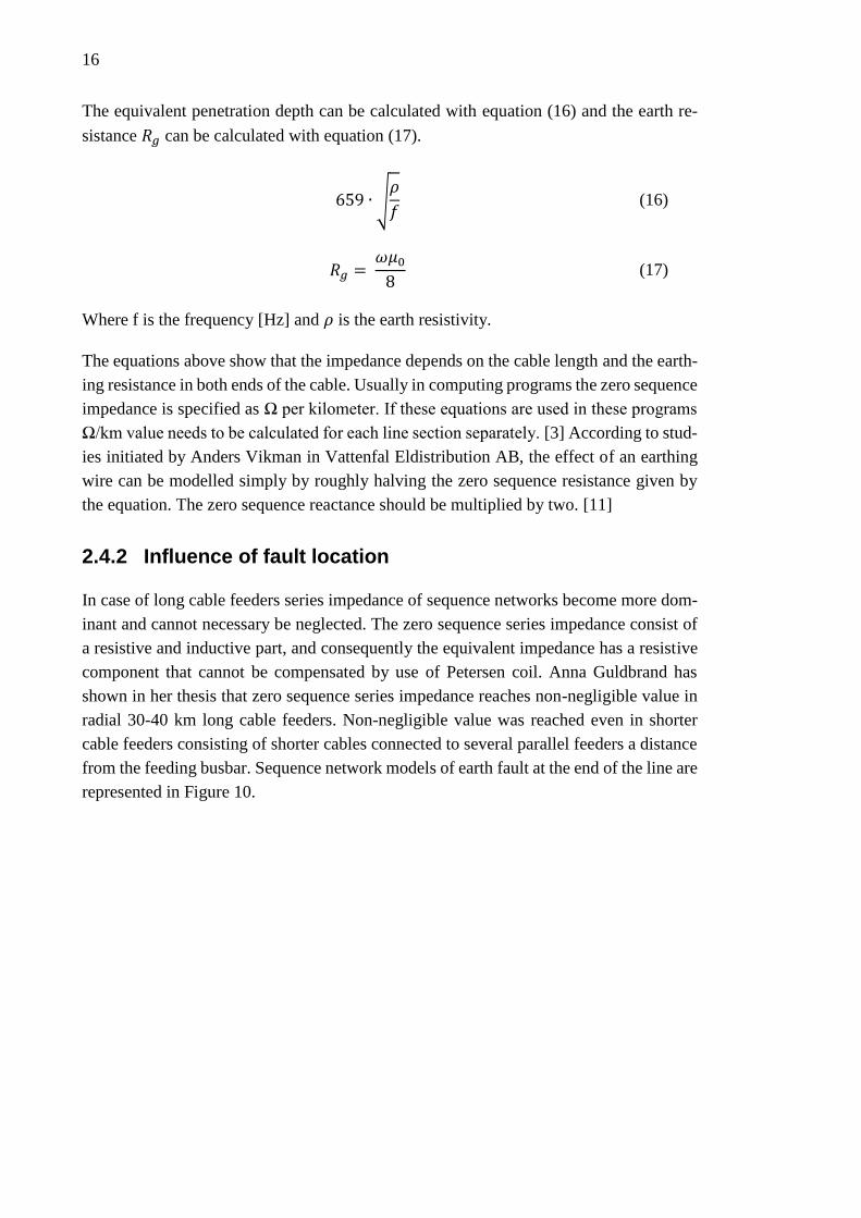
The equivalent penetration depth can be calculated with equation (16) and the earth re-
sistance 𝑅𝑔 can be calculated with equation (17).
659 ∙ √𝜌
𝑓 (16)
𝑅𝑔 = 𝜔𝜇0
8 (17)
Where f is the frequency [Hz] and 𝜌 is the earth resistivity.
The equations above show that the impedance depends on the cable length and the earth-
ing resistance in both ends of the cable. Usually in computing programs the zero sequence
impedance is specified as Ω per kilometer. If these equations are used in these programs
Ω/km value needs to be calculated for each line section separately. [3] According to stud-
ies initiated by Anders Vikman in Vattenfal Eldistribution AB, the effect of an earthing
wire can be modelled simply by roughly halving the zero sequence resistance given by
the equation. The zero sequence reactance should be multiplied by two. [11]
2.4.2 Influence of fault location
In case of long cable feeders series impedance of sequence networks become more dom-
inant and cannot necessary be neglected. The zero sequence series impedance consist of
a resistive and inductive part, and consequently the equivalent impedance has a resistive
component that cannot be compensated by use of Petersen coil. Anna Guldbrand has
shown in her thesis that zero sequence series impedance reaches non-negligible value in
radial 30-40 km long cable feeders. Non-negligible value was reached even in shorter
cable feeders consisting of shorter cables connected to several parallel feeders a distance
from the feeding busbar. Sequence network models of earth fault at the end of the line are
represented in Figure 10.

17
Figure 10. Sequence networks representing an earth fault at the end of the line with
negligible (left) and non-negligible (right) series impedances of sequence networks [3]
In the left figure the series impedances of positive, negative and zero sequence networks
are neglected as in conventional earth fault analysis. In right figure the series impedances
are non-negligible, which causes voltage drop in sequence networks. Since the voltage
drop has a real and imaginary part, the zero sequence voltage magnitude can either in-
crease or decrease. In Figure 11 the neutral point displacement voltage and zero sequence
voltage at fault location is presented during an end of line fault with different line lengths.
Figure 11. Neutral point displacement voltage (dashed) and zero sequence voltage at
fault location (solid) during an end of line fault in resonance earthed system. Phase is
related to the neutral point displacement voltage. [3]
Since there are voltage drops across the non-negligible series impedances of the faulted
feeder, the amplitude and the phase of neutral point displacement voltage are different
from that of the zero sequence voltage at the fault location. The voltage drop depends on
the size and phase of zero sequence current but also the size and phase of equivalent zero

18
sequence impedance and hence depends on the network structure and location of the fault.
In addition, the voltage drops in positive and negative sequence networks influence the
zero sequence voltage at the fault location. This causes that the zero sequence voltage at
the fault point differs from the phase voltage, even if the fault impedance is negligible.
[3]
Since the maximum earth fault current is considered as the worst case scenario, it is there-
fore consequential to find the fault location in which the earth fault current reaches its
maximum value. Figure shows the earth fault current during busbar fault and end of line
fault in resonance earthed system tuned for faults in busbar. IR is the resistive earth fault
current component and IC is the capacitive earth fault current component.
Figure 12. Fault currents at the fault location during solid busbar earth fault (solid)
and solid earth fault at end of the line (dashed) in resonance earthed rural cable system
with variable cable lengths [3]
The curves in Figure 12 shows that fault current during an end of line fault is smaller than
fault current during busbar fault. This is because the positive and negative impedance
contribute to the equivalent impedance, which limits the earth fault current. Even though
the calculations show that the earth fault current is larger for faults in busbar than faults
in end of line, it cannot be concluded that a fault on the busbar gives maximum earth fault
current. The Petersen coil decreases the earth fault current but since it cannot be tuned to
compensate same amount of earth fault current independently on fault location, the influ-
ence of earthing will vary depending on fault location. [3] As mentioned above the effect
on fault location on the earth fault current and neutral point displacement voltage is due
to series impedances of sequence networks. The effect of series impedances can be min-
imized by use of distributed compensation described in Section 2.5.2.

19
2.5 Earth fault current compensation
2.5.1 Centralized compensation
In Finnish networks the high voltage side of the primary transformer is earthed only in
some particular points defined by Fingrid Oyj, but basically the transmission network is
unearthed. As a result the earth fault in transmission network does not effect on the cur-
rents or voltages in the medium voltage network. Same applies in case of earth fault in
medium voltage network: it does not effect on the primary side network of primary trans-
former. The primary transformers are mainly Yd coupled, which means that there is no
neutral point in secondary side available. Therefore in order to connect an earthing device
to neutral point of medium voltage network a neutral point needs to be created. This is
usually done with earthing transformer, which usually is Znyn-coupled. The compensa-
tion coil is connected to neutral point of earthing transformer via disconnector that ena-
bles the disconnection of the coil during for example maintenance. The centralized Pe-
tersen coil is automatically adjustable. In Finland compensation degree is kept slightly
under compensated, but for example in Sweden it is kept slightly overcompensated. Be-
hind this practice is the idea that it is more likely for some network part to be disconnected
from network, which changes the network closer to resonance point. [11]
2.5.2 Distributed compensation
Instead of one large controlled coil in the HV-MV substation it is possible to install small
compensation devices around the system. Each of these devices comprises a star point
transformer and Petersen coil without automatic control or transformer that consist of YN
connected Petersen coil for earth fault current compensation and distribution transformer
[10]. Distribution transformers with only earth fault current compensation capability are
Zn(d)yn or Znzn0-coupled. These couplings give the magnetic balance to the transformer
in case of an earth fault at LV-side of distribution transformer, which disables the earth
fault current to be seen in MV-voltage side. [11] If these coils are properly located in
individual feeders around the network, no additional automatically adjusted arc-suppres-
sion-coil is required. The disconnection of the compensation equipment when the associ-
ated feeder is isolated from the network keeps the compensation level at sustainable state
regardless of the switching arrangements on the network. [1]
2.5.2.1 Effect of distributed compensation on earth fault current
transportation
In system where series reactance can be neglected, equivalent circuit of earth fault in
system with distributed compensation is equal to one in case of system with centralized
compensation except that zero sequence network consists of multiple parallel inductances

20
and possible resistances. Earth fault current and neutral point displacement voltage can
be calculated with equations (6) and (7) presented in Section 2.1.2.
The distributed compensation is one solution to limit the resistive losses caused in trans-
portation of reactive current and non-ideal neutral point reactors. In Figure 13 the se-
quence networks in case of earth fault in busbar is presented. In system presented in left
side of the figure only centralized compensation coil is used. In the system presented in
the right side of the figure combination of centralized and distributed compensation is
used.
Figure 13. Earth fault at the busbar in single long cable system with centralized (left)
and distributed compensation (right) [3]
If the cable is long and only centralized compensation is used the zero sequence series
impedance is not negligible. If also distributed coils are used and those are dimensioned
to compensate for the capacitive current generated in the system, and the distance between
the coils is limited, the total shunt impedance is very large and the series impedance can
therefore be neglected. [3]
2.5.2.2 Coil rating
The effect of arc suppression coils is based on the inductive earth fault current generated
in the coil, which compensates the capacitive earth fault current. Distributed compensa-
tion coils are manually adjustable and there are coils of different sizes. ABB produces
coils with compensation capacity of 3,5 - 5 A, 5 - 15 A and 15 - 25 A. [10] The rating of
the coil can also made by the shunt impedances of the system. For the influence of series
impedance of the system to be as small as possible, the equivalent zero sequence shunt
impedance should be as large as possible. The shunt reactance of system can be calculated
with equation (18).

21
𝑋𝑠ℎ𝑢𝑛𝑡 =𝜔3𝐿𝑙𝑜𝑐𝑎𝑙 ∙
1𝜔𝐶0𝑥𝑘𝑚
1𝜔𝐶0𝑥𝑘𝑚
− 𝜔3𝐿𝑙𝑜𝑐𝑎𝑙
(18)
Where Xshunt is the shunt reactance of compensated line section, 𝐿𝑙𝑜𝑐𝑎𝑙 is the inductance
of distributed coil and 𝐶0𝑥𝑘𝑚 is the equivalent capacitance of the cable section.
While the reactance of coil approaches the reactance of cable section the total shunt reac-
tance approaches infinity. In reality the capacitance to earth is distributed and the shunt
admittance is therefore finite. As the distance between coils increases, shunt admittance
of the system decreases and resistive losses in zero sequence network increases. [4] In
addition to resistive losses of in lines resistive losses are also generated in compensation
coils. Resistive losses of compensation coils are approximately 2,5 % and therefore losses
increases while the coil size increases. [10] The current provided by compensation coil
can be calculated with equation (19).
𝐼𝐿 =𝑈0
√3∙
1
𝑅𝐿 + 𝑗𝜔𝐿 (19)
Where 𝑈0 is the zero sequence voltage affecting on distributed coil, 𝑅𝐿 is the series re-
sistance of the coil and L is the inductance of the coil.
2.5.2.3 Coil location
The location of distributed arc suppression coils effects on the resistive losses during earth
fault. It is recommended in Licentiate thesis of Anna Guldbrand that 15 to 20 km of each
cable feeders are compensated by centralized compensation coil and the rest of the feeders
are compensated with local compensation coils.
In reference [13] J. Jaakkola and K. Kauhaniemi have been investigated the effect of
density of distributed coil. In that paper the smallest variation in fault currents in different
fault locations was reached in distributed compensated networks where distributed coils
were placed in 5 km intervals. However, there was no big difference compared to situation
where coils were placed in 10 km or 20 km intervals. Therefore it is probably cost efficient
to install coils with 10 or 20 km intervals. In case of centralized and distributed coils it
turned out to be good solution to compensate first 10 km of feeders with centralized com-
pensation coil and the rest of the feeders with distributed coils with interval of 10 km.
[13]
During a pilot project in Savon Voima Verkko Oy Dyn11+YN coupled distributed coils
were installed in cabled rural distribution network. Esa Virtanen proposes that on the basis
of experience in that project the optimum location of coils is about 10 km from each
other’s, and that in mixed network 50 % of earth fault current should be compensated
centrally and 50 % with distributed coils. [10]

22
2.6 Analysis method for compensated system equipped with
distributed coils
In above sections it have been demonstrated that the assumptions of conventional earth
fault analysis cannot be used in system consisting of long cable feeders. In addition to the
series resistances of long feeders the increased amount of resistive losses in distributed
coils and in zero point transformers causes inaccuracy to conventional analysis. Gunilla
Brännman has developed a method in which the resistance of distributed coils and the
zero sequence impedance of transformer are taken into consideration. The model is de-
veloped based on symmetrical components and is explained more detail in publication
“Analysmodell för Impedansjordat System med Lokal Kompensering”. In this section the
basics of the modeling method are presented. [14]
In conventional earth fault analysis only the shunt capacitances and shunt reactance of
zero sequence network are taken into consideration. In this modeling method only imped-
ances which have smaller effect than 1 % into total impedance are neglected. The positive
sequence impedance is the impedance of network that participates the short circuit in the
system. Negative sequence impedance is usually equal to positive sequence impedance
in case of lines and transformers. Zero sequence impedance depends mainly on the earth-
ing of the system. In order to present the idea of the method the sequence networks are
created for system consisting of two feeders A and B. There is a centralized compensation
coil in the neutral point of primary transformer and two distributed coils are placed in
feeder B. Dyn coupled transformer in feeder A is a normal distribution transformer. The
system is presented in Figure 14.
Figure 14. System consisting of two feeders. Earth fault occurs in feeder A. [14]
In case of a single phase earth fault on feeder A the equivalent positive and negative
sequence impedances look like one presented in Figure 15. The positive sequence re-
sistance of primary transformer and feeder B is in this case neglected. Every line sections
are modelled with pi-section consisting of shunt capacitances and series impedance.

23
Figure 15. The equivalent circuit of positive and negative sequence networks in case of
a single phase earth fault in feeder A [14]
In Figure 15 Xnät is the impedance of supply point, XT1 is the positive sequence impedance
of primary substation, Xca is the positive sequence capacitive reactance of feeder B, Xc is
the positive sequence capacitive reactance of feeder A, Rl is the positive sequence re-
sistance of feeder A, Xl is the positive sequence reactance of feeder A.
The zero sequence impedance of the system can be calculated from equivalent circuit
presented in Figure 16.
Figure 16. The equivalent circuit of zero sequence network in case of a single phase
earth fault in feeder A [14]
In Figure 16 Xn is the reactance in the neutral point, Rn is the resistance in the neutral
point, X0T1 is the zero sequence reactance of primary transformer or zero point trans-
former, Z0a is the total zero sequence impedance of feeder B, X0c is the zero sequence
capacitive reactance of feeder A, R0l is the zero sequence resistance of feeder A, X0l is the
zero sequence inductive reactance of feeder A.
The total zero sequence impedance of feeder B consists of modules, including locally
compensated line sections and distributed coils, and pi-sections of lines that are not lo-
cally compensated. The impedance of feeder B is presented in Figure 17.

24
Figure 17. The equivalent circuit for the zero sequence impedance of feeder B.
Corresponds Z0a in Figure 16 [14]
In Figure 17 X0ca is the zero sequence capacitive reactance of feeder B before the first
cable/distributed coil –module, R0la is the zero sequence resistance and X0la is the zero
sequence inductive reactance respectively. Zu is the zero sequence impedance of ca-
ble/distributed coil –module which is presented more detail in Figure 18.
Figure 18. The equivalent circuit of the zero sequence impedance of the module con-
sisting of distributed compensation coil and locally compensated line sections. Circuit
corresponds Zu in Figure 17 [14]
In Figure 18 X0ckabel is the zero sequence capacitive reactance of cable in cable-coil mod-
ule, X0T2 is the zero sequence inductive reactance of zero point transformer, R0T2 is the
zero sequence resistance of zero point transformer, Xnu is the zero sequence inductive
reactance of distributed arc suppression coil and Rnu is the zero sequence resistance of
distributed arc suppression coil. As can be seen in Figure 18 the series impedance of the
locally compensated line section is neglected.
In systems that consists of multiple distributed arc suppression coils in the feeder, the
total impedance of cable-coil modules is the inductance of parallel connection of those
modules. In case the arc suppression coils are similar to each other the total impedance
of n modules is Zu/n.
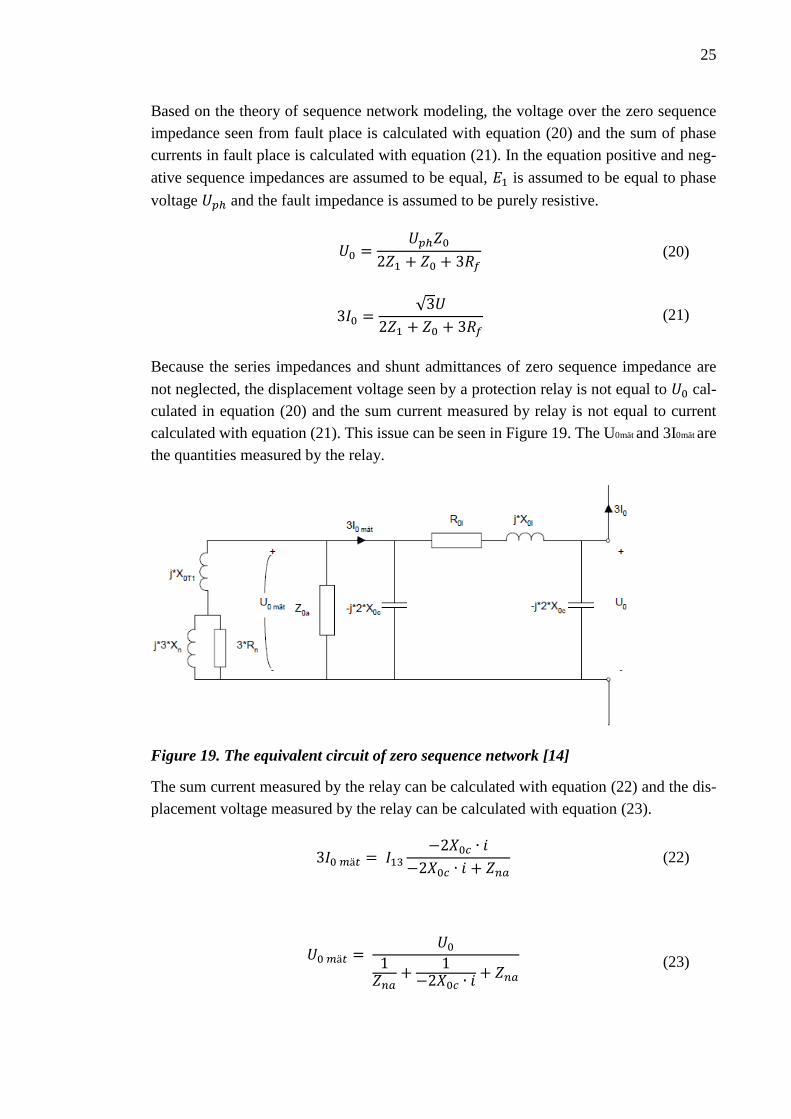
25
Based on the theory of sequence network modeling, the voltage over the zero sequence
impedance seen from fault place is calculated with equation (20) and the sum of phase
currents in fault place is calculated with equation (21). In the equation positive and neg-
ative sequence impedances are assumed to be equal, 𝐸1 is assumed to be equal to phase
voltage 𝑈𝑝ℎ and the fault impedance is assumed to be purely resistive.
𝑈0 =𝑈𝑝ℎ𝑍0
2𝑍1 + 𝑍0 + 3𝑅𝑓 (20)
3𝐼0 =√3𝑈
2𝑍1 + 𝑍0 + 3𝑅𝑓 (21)
Because the series impedances and shunt admittances of zero sequence impedance are
not neglected, the displacement voltage seen by a protection relay is not equal to 𝑈0 cal-
culated in equation (20) and the sum current measured by relay is not equal to current
calculated with equation (21). This issue can be seen in Figure 19. The U0mät and 3I0mät are
the quantities measured by the relay.
Figure 19. The equivalent circuit of zero sequence network [14]
The sum current measured by the relay can be calculated with equation (22) and the dis-
placement voltage measured by the relay can be calculated with equation (23).
3𝐼0 𝑚ä𝑡 = 𝐼13
−2𝑋0𝑐 ∙ 𝑖
−2𝑋0𝑐 ∙ 𝑖 + 𝑍𝑛𝑎 (22)
𝑈0 𝑚ä𝑡 = 𝑈0
1𝑍𝑛𝑎
+1
−2𝑋0𝑐 ∙ 𝑖 + 𝑍𝑛𝑎
(23)

26
In which
𝐼13 = 3𝐼0
−2𝑋0𝑐 ∙ 𝑖
−2𝑋0𝑐 ∙ 𝑖 + 𝑍02
𝑍02 = 1
1𝑍𝑛𝑎
+1
−2𝑋0𝑐 ∙ 𝑖
+ 𝑅0𝑙 + 𝑋0𝑙 ∙ 𝑖
𝑍𝑛𝑎 = 1
1𝑍𝑛
+1
𝑍0𝑎
In the above equations 𝑍𝑛 is the total impedance consisting of impedance of centralized
coil and the zero sequence impedance of transformer.
This method is more accurate way to model the earth fault behavior of system consisting
distributed compensation coils and long cables. The effect of coil size, resistive losses
and the series impedances of lines are now taken into consideration. It is however hard to
accurately define the zero sequence parameters of lines and devices, which makes it hard
to model the behavior of the systems accurately. [14]

27
3. REACTIVE POWER CONTROL
3.1 Objectives of reactive power compensation
Investments of distribution networks are expensive and the lifetimes of network compo-
nents are long. That is why investments need to be carefully designed to make sure that
resources are used effectively. When different network investment plans are compared
both technical and economic issues need to be taken into consideration. In this section
technical and economic factors that effects on reactive power compensation method are
presented.
3.1.1 Power losses
Reactive power is the second component of electrical power. Some loads need reactive
power but transferring reactive power causes unnecessary losses in power lines and trans-
formers. Apparent power is the complex sum of reactive and active powers, which is why
the excess of reactive power Q increases the demand of apparent power. According to
Ohm’s law the power of electric circuit depends on voltage and current. Since the voltage
of transmission network is kept constant the current has to grow to enable apparent power
to increase. Growth of current causes active losses in lines. Active power losses Ploss of a
line is calculated using equation (24).
𝑃𝐿𝑜𝑠𝑠 = 3𝐼2𝑅 (24)
Where I is the phase current flowing in a transmission line and R is the series resistance
of the line. Since the current of transmission line consist of reactive and active compo-
nents, equation (24) can be derived into equation (25).
𝑃𝑙𝑜𝑠𝑠 = (𝑃
𝑈)
2
𝑅 + (𝑄
𝑈)
2
𝑋 (25)
Where X is the series reactance of the transmission line and U is the voltage of the net-
work in examined point. [15]
It can be seen in both equations above that reactive power noticeably effects on the losses
of transmission line. As the reactive power increases the current in transmission line, it
also reduces the transferring capacity of the line. Transferring capacity of cable is deter-
mined by thermal limits. Another concern is the load losses of primary transformer. The
losses in primary transformer are also dependent on the apparent power flow.

28
3.1.2 Voltage rise
Voltage drop along the feeder depends on the line’s impedances and the load current
flowing through the line. In a single radial lightly loaded circuit homogenously distributed
phase to earth capacitance feeds reactive power to circuit and the voltage drop is therefore
having a negative value proportional to the square of circuit length. An inductive reac-
tance of power line consumes reactive power and the shunt capacitances of the line gen-
erate it. The amount of generated reactive power is proportional to voltage of the line.
The amount of consumed reactive power in the series inductive reactance is proportional
to the current flowing through the line. The total reactive power generated by three phases
can be calculated with equation (26).
𝑄𝐶 = 3𝑈𝑝ℎ2𝐵 (26)
Where Uph is the phase voltage and B is the capacitive susceptance of the line. The total
amount of reactive power consumed in three phases of power line can be calculated with
equation (27).
𝑄𝐿,𝑙𝑖𝑛𝑒 = 3𝐼2𝑋𝐿𝑖𝑛𝑒 (27)
Where I is the current flowing through the line and XLine is the inductive series reactance
of the line.
Power line is working on its natural loading if the generated and consumed reactive pow-
ers are equal. In this case the power line compensates itself, which means the power line
takes no reactive power from elsewhere. Equations (26) and (27) can now set equal as in
equation (28).
𝑄𝐶 = 𝑄𝐿,𝑙𝑖𝑛𝑒 ⇔ 3𝑈𝑝ℎ2𝐵 = 3𝐼2𝑋𝐿 ⇔
𝑈𝑝ℎ2
𝐼2=
𝑋𝐿
𝐵=
𝐿
𝐶= 𝑍𝐶
2 (28)
Where ZC is the impedance of the load needed to operate power line on its natural loading.
If both side of the equation is squared, it results equation (29).
𝑍𝐶 = √𝐿
𝐶 (29)
With this load impedance, the power line operates on its natural loading. According to
the theory of transmission lines the best transmission condition is achieved in case the
impedance of the load equals to the characteristic impedance of the line. This means that
ZC can also be called the characteristic impedance. ZC is actually a phasor with angle, but
in case of lossless line equation (29) is valid and the voltage profile is flat through the
line. The surge impedance loading (SIL) is amount of real power that is needed to operate

29
power line in its natural loading. Surge impedance loading can be calculated with equa-
tion (30).
𝑆𝐼𝐿 = 𝑈2
𝑍𝐶 (30)
Surge impedance loading is considerably higher for cables compared with overhead lines
because the higher values of capacitance. In distribution network the SIL of the cable is
approximately 10 times larger than the SIL of an overhead line [16]. At least in case of
transmission network cables the current carrying capacity limits the transferred load be-
fore the natural loading is achieved. This is why cables are operated below its SIL and
the cables are therefore generating reactive power [17] [16].
3.1.3 Reactive power fee
The power system in Finland consists of power plants, main grid, regional networks, dis-
tribution networks, and consumers of energy. Fingrid Oyj is the owner of main grid in
Finland. Fingrid is responsible for operation supervision, operation planning, mainte-
nance and development of the main grid and for electricity market development.
Fingrid is attending to the reactive power balance to maintain voltage levels in sustainable
level. In order to encourage DSOs to keep the reactive power in limits, Fingrid inherits
fees for exceeding reactive power limits. The use of reactive power is monitored prelim-
inary at a regional level. Regions are created from customer’s or customers’ connection
points which are close to each other electrically. When the reactive power limits of a
regional monitoring area are exceeded and it disturbs the operation of the main grid, Fin-
grid has the right to invoice the owner of the connection point. [18]
The output limit of reactive power at the connection point is calculated using formulas
(31). The formula that results higher value is chosen to be the output limit on the basis of
the calculation.
𝑄𝑆 = 𝑊𝑜𝑢𝑡 ∙0,16
𝑡𝑘+ 0,025 ∙
𝑊𝑝𝑟𝑜𝑑
5000
𝑄𝑆 = 𝑊𝑜𝑢𝑡 ∙0,16
𝑡𝑘+ 0,1 ∙ 𝑆𝑁
(31)
Where 𝑊𝑜𝑢𝑡 is the output energy (MWh) at the connection point, 𝑊𝑝𝑟𝑜𝑑 is the net pro-
duction (MWh) of the power plant at the connection point, 𝑆𝑁 is the apparent power of
largest generator at the connection point and 𝑡𝑘 is the peak usage time, which is defined
for different consumption type. Peak usage times for consumption types are following
represented in Table 2.

30
Table 2. Peak usage times for consumption types [19]
𝒕𝒌 (h) Consumption type
7000 Process industries
6000 Other industries
5000 Other consumption
If the largest generator is smaller than 10 MVA 𝑊𝑝𝑟𝑜𝑑= 0 and 𝑆𝑁= 0. 0,1∙𝑆𝑁 is however
at most 30 MVAr. The input limit of reactive power at the connection point is calculated
using the equation (32).
𝑄𝑆1 = −0,25 ∙ 𝑄𝑆 (32)
The reactive power fee consist of usage fee and energy fee. The reactive power fee is
determined on the basis of the highest exceeding of the reactive power window in a
month. Energy fee is 10 €/MVArh for all reactive power that is supplied or received
in/from the area that is exceeding the reactive power window in the month. The reactive
power window and the fees to be paid for exceeding the use of reactive power are pre-
sented in Figure 20. Fees are calculated using following equations (33), (34) and (35):
If P ≤ QS / 0,16 and Q > QS
(𝑄 − 𝑄𝑆) ∙ 3000 €/𝑀𝑉𝐴𝑟 (33)
If P ≤ QS / 0,16 and Q/P > 0,16
(𝑄 − 0,16 ∙ 𝑃) ∙ 3000 €/𝑀𝑉𝐴𝑟 (34)
If |Q| > |QS1|
(|𝑄| − |𝑄𝑆1|) ∙ 3000 €/𝑀𝑉𝐴𝑟 (35)
Q is the reactive power in the high voltage side of connection point in the examination
hour. If the reactive power measurement QM is in low voltage side Q = QM – QL where
QL is the calculated reactive power losses of transformers and branch lines at the connec-
tion point. P is measured average power of active power at the connection point during
the examination hour.

31
Figure 20. Reactive power window [19]
If the output or input of reactive power exceeds the reactive power window, the reason
for exceeding shall be verified before potential invoicing. The exceeding of the window
shall not be invoiced if the exceeding is caused by a fault or disturbance in the main grid.
If the window have not been exceeded more than 10 hours per month and the output or
input reactive power have not exceeded doubly the supply limit, no reactive power fees
will be charged for that month. [19]
Reactive power fee contract is at the moment open to interpretation. Fees are not based
on real expenses and it has been hard to reveal the source of exceeding reactive power
window because there might have been multiple connection points of different DSOs in
the same monitoring area. Because the extending use of cable in distribution network
effects on reactive power generation, some changes are going to be made in main grid
contract. In new contract that will be taking effective in beginning of 2016, reactive power
fees are based on real expenses and connection points are going be monitored and charged
separately. [20] Reactive power fees will be based on the expenses of investing costs of
reactors, capacity that reactive power reserves and maintenance costs of compensators.
Reactive energy fee will be based on the losses of compensators and the losses in the
feeders caused by reactive power. Costs will also be checked annually. Any official num-
bers have not been published but in reference [21] new cost for exceeding reactive power
fees have been suggested. Suggested fees are
Reactive power consumption: 1000 €/MVAr, month
Reactive power production: 1500 €/MVAr, month
Reactive energy: 5 €/MVArh

32
Even though fees would be smaller than earlier, since reactive power window will be
formed for every connection point, DSOs need to pay more attention on the monitoring
of reactive power window to avoid reactive power fees.
3.2 Compensation devices
Preventing unnecessary reactive power flow in network is possible by generating reactive
power where it is consumed, or on the contrary, consume reactive power where it is gen-
erated. In some countries feeder capacitors are commonly used to generate reactive power
for purposes of lines and consumers but in Nordic countries these are rare. Capacitors are
mainly located in substations to control reactive power flow through primary transformers
to avoid reactive power charges from the transmission system operator (TSO). [22] Con-
trarily to overhead line network in cable network reactive power needs to be consumed
to prevent unnecessary reactive power flow. Reactive power can be consumed with shunt
reactors connected parallel to the lines.
3.2.1 Shunt capacitors
Shunt capacitors are used to compensate inductive reactive power. Capacitors are quite
common in HV-MV substations that are feeding overhead lines. While cabling of distri-
bution network increases the need for capacitors in substations decreases at least if the
loads of substation are easily predictable and load profile is flat. HV shunt capacitor bank
consists of multiple parallel and series connected standard sized capacitor banks. Capac-
itor banks are typically 20 – 50 MVAr in 110 kV networks and 1-5 MVAr in 20 kV
networks. Reactive power generated by capacitor can be calculated with equation (36)
[15].
𝑄𝑐𝑎𝑝 = 𝜔𝐶𝑈2 = (𝑈
𝑈𝑁)
2
𝑄𝑁 (36)
Where ω is the angular frequency, UN is the nominal voltage of a capacitor, QN is the
nominal reactive power of a capacitor and U is the voltage of the network.
As can be seen from equation (36) the reactive power generated by shunt capacitor fluc-
tuates dramatically if voltage decreases. In case of a fault in power system feeder is sep-
arated from network. Thus the reactive power of system decreases and reactive power
support is needed. While reactive power decreases also the voltage in network decreases.
Thus also the reactive power generated by capacitor decreases. Above described scenario
is why shunt capacitors poorly fit for reactive power support of power system while fault.
[15]

33
3.2.2 Shunt reactors
Reactors are electrically the opposite of capacitors. Reactors are used to consume reactive
power. Reactors can also be used to filter harmonics or to limit current. There are several
possible connection choices for reactors used in reactive power compensation: delta-con-
nection, unearthed wye-connection, earthed wye-connection and earthed wye connection
with a neutral reactor. [23] The latter is used only in countries where one phase reclosing
is used. The purpose of reactor between star point and earth is to compensate the second-
ary arc current flowing from healthy line to faulted line during earth fault that might pre-
vent the successful reclosing [15].
Delta-connection and unearthed wye-connection can be transformed to each other with
wye-delta transformation. These unearthed reactor connections affects only in reactive
power of line while reactors with earthed star point compensates also the earth fault cur-
rent of the system. The reactance of wye connected reactor can be calculated with equa-
tion (37) and the reactance of delta connected reactor can be calculated with equation
(38).
𝑋𝑤𝑦𝑒 = 𝑈𝑁
2
𝑆𝑅3𝛿
=𝑈𝑁
2
3 ∙ 𝑆𝑅1𝛿
(37)
𝑋𝑑𝑒𝑙𝑡𝑎 = 3 ∙𝑈𝑁
2
𝑆𝑅3𝛿
=𝑈𝑁
2
𝑆𝑅1𝛿
(38)
Where 𝑈𝑁 is the nominal system voltage, 𝑆𝑅3𝛿 is the rated three-phase reactive power,
𝑆𝑅1𝛿 is the rated reactive power per phase. [23]
Reactive power consumed by shunt reactor can be calculated using equation (27), equa-
tion (39) or equation (40):
𝑄 =3𝑈𝑐𝑜𝑖𝑙
2
𝑋𝑝ℎ (39)
𝑄 = (𝑈
𝑈𝑁)
2
𝑄𝑁 (40)
Where Q is the reactive power that shunt reactor consumes, Ucoil is voltage over the each
coil, Xph is reactance of individual coil in shunt reactor, U is voltage over shunt reactor
and UN is rated voltage of shunt reactor and QN is rated power of reactor.

34
3.2.3 FACTS devices
In networks where consumption and generation are reasonably predictable and stable,
fixed shunt capacitor banks or fixed shunt reactors are used. Reactive power compensa-
tion is then accomplished for a specific operation condition only. Mechanical switching
of those units offers more flexibility in the system.
In the situation where loads change rapidly, for example in electric arc furnaces, rapid
voltage changes can cause disturbances in lightning systems and in other power equip-
ment. In such cases Static Var Compensation (SVC) installations are provided. SVC con-
sists of thyristor controlled reactor in parallel to a fixed capacitor bank. It provides a fast
controllable reactive load which responds very quickly to voltage changes. [24] Like an
SVC, Static Compensator (STATCOM) instantly and continuously provides variable re-
active power in response to voltage transients, supporting the stability of grid voltage. A
small STATCOM can also be combined with switched passive elements to more econom-
ically have a controllable reactive power compensator. [25]
If very fast and dynamic response is not mandatory, a continuously Variable Shunt Reac-
tor (VSR) may be optimal choice for reactive power compensation. VSRs are favored in
networks with distributed generation whose may not always provide full control over their
electrical output and in networks with strongly varying loads powered through long over-
head lines or cables. As a part of the overall reactive compensation scheme, a continu-
ously VSR may provide reactive power compensation and smooth steady state voltage
control in response to the daily load cycle and possible changes in power generation.
Because the consumed reactive power of VSRs is not fixed, it offers the ability to adapt
to system topology changes. [26]
The adjustability of VSRs power output is obtained via variation of its inductance, which
is achieved by adjusting the air gaps of its magnetic circuits. In order to apply the auto-
matic control of the VSR an automatic control device is needed to control the motor drive
unit for coil adjustment. For example Trench’s control device is used both in earth fault
compensation controller and in VSR reactive power controller that allows remote opera-
tion of the VSR by means of digital inputs or via a substation automation and control
system. [26]. The compensation ability of different compensation devices in function of
voltage is presented in In Figure 21.

35
Figure 21 Reactive current versus the connected voltage of different reactive power
compensation devices [24]
Reactive power of passive components is dependent on voltage and the reactance of the
component, but reactive power of STATCOM and SVC have much larger ability to
change the generated reactive power in different voltage conditions.
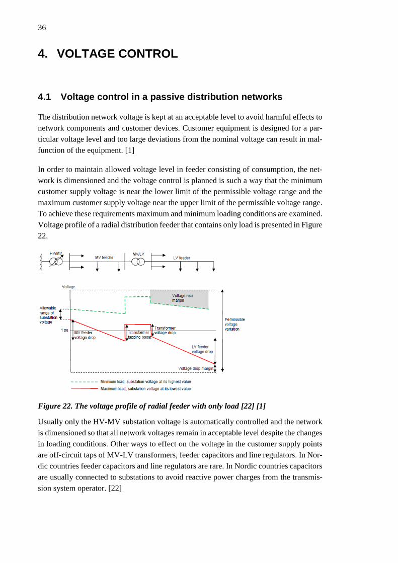
36
4. VOLTAGE CONTROL
4.1 Voltage control in a passive distribution networks
The distribution network voltage is kept at an acceptable level to avoid harmful effects to
network components and customer devices. Customer equipment is designed for a par-
ticular voltage level and too large deviations from the nominal voltage can result in mal-
function of the equipment. [1]
In order to maintain allowed voltage level in feeder consisting of consumption, the net-
work is dimensioned and the voltage control is planned is such a way that the minimum
customer supply voltage is near the lower limit of the permissible voltage range and the
maximum customer supply voltage near the upper limit of the permissible voltage range.
To achieve these requirements maximum and minimum loading conditions are examined.
Voltage profile of a radial distribution feeder that contains only load is presented in Figure
22.
Figure 22. The voltage profile of radial feeder with only load [22] [1]
Usually only the HV-MV substation voltage is automatically controlled and the network
is dimensioned so that all network voltages remain in acceptable level despite the changes
in loading conditions. Other ways to effect on the voltage in the customer supply points
are off-circuit taps of MV-LV transformers, feeder capacitors and line regulators. In Nor-
dic countries feeder capacitors and line regulators are rare. In Nordic countries capacitors
are usually connected to substations to avoid reactive power charges from the transmis-
sion system operator. [22]

37
The voltage level in substation is usually adjusted by AVC relay. At the simplest, the
AVC relay aims to keep the substation voltage constant. The AVC relay compares the
measured substation voltage and the reference voltage. If the reference voltage differs
from measured voltage more than the AVC relay dead band, the delay counter is started.
The delay counter remains active as long as the measured voltage remains outside the
hysteresis limit of the AVC relay. The delay can use definite or inverse time characteris-
tics. Modern AVC relays have a possibility to use line-drop compensation as standard. In
line-drop compensation the substation voltage is not kept constant but it depends on the
current flowing through the main transformer. The measured substation voltage VSS is
replaced with VSS -(R+jX)*I, where (R+jX) is the line impedance between the substation
and the load centre which voltage is wanted to kept constant. I is the current of main
transformer. [22]
The MV-LV transformers of the have off-circuit taps that can be used to change the wind-
ing ratio of the transformers. To change the setting of these taps interruption of electricity
supply is needed, which is why their position is decided at the planning stage and kept
constant throughout the year. [22]
4.2 Distributed generation in a passive distribution network
In Figure 22 unidirectional power flows have been assumed when voltage control has
been planned and, therefore, the margin to the feeder voltage upper limit is relatively
small. When generation is connected to network, unidirectional power flow cannot be
assumed and the voltage profile of the network can become quite different as presented
in Figure 23.

38
Figure 23. The voltage profile of a radial feeder when also generation is present [22].
When generation is connected on the MV-feeder, the feeder might have sections with
both ascending and descending voltage profiles. In maximum loading conditions genera-
tion rises the voltage and hence improves the voltage. During minimum loading, maxi-
mum generation conditions, the maximum voltage exceeds the feeder voltage upper limit
and the voltage performance of the feeder is not acceptable.
At the moment distributed generation (DG) is not allowed to participate in network con-
trol in any way. Two extreme loading conditions are considered and if voltage becomes
excessive passive methods are used to lower the distribution network maximum voltage
to an acceptable level. Usually conductor size is increased or generation is connected on
a dedicated feeder. [22]
4.3 Active voltage level management
Voltage rise caused by DG is usually the factor that limits the hosting capacity for DG.
The voltage rise can be reduced by decreasing line impedance, by controlling the real and
reactive power flows in the network or by adjusting the substation voltage at some point
along the feeder. Methods to decrease the maximum supply point voltage is listed in the
following:
Increasing conductor size
Connecting generation on a dedicated feeder
Adjusting the off-circuit taps of the MV-LV transformers
Installing step voltage regulators on feeders
Reducing substation voltage
Allowing the generator to absorb reactive power
Allowing the curtailment of generator real power
Installing passive or active reactive power compensators on feeders
Controlling the loads
Installing energy storages and charging them when voltage rise needs to be miti-
gated
Coordinated voltage control (CVC) methods determine their control actions based on the
state of the whole distribution network and controls the controllable resources to maintain
voltages in acceptable limits. The CVC methods can determine their control actions based
on control rules or use some kind of optimization algorithm. The import data can be di-
rectly measured or state estimation can be utilized. Coordinated voltage control methods
could be categorized also based on the control variables they use in the control. The most
common control variables are substation voltage and real and reactive powers of DG
units. [22]

39
The optimizing algorithms can be categorized based on the objective function. Possible
variables to be minimizes by CVC algorithm are network losses, DG real power curtail-
ment, cost of reactive power control, cost of reactive and real power import from the
transmission system, number or cost of tap changer operations and quantities related to
voltage quality such as average voltage deviation and maximum voltage deviation. [22]
There are quite big difference in how easily different kinds of active resources can be
taken into voltage control use. Production curtailment of DG units can be taken into use
relatively easily if equipment needed for remote real power control already exists. How-
ever electricity distribution and production are unbundled and the DSO is not responsible
for dispatching the DG units. Contracts needs to be made to allow the DSO to control real
power of DG units. In case of load control, the equipment to control loads needs to be
installed because no such equipment usually exists. Also contracts with customer needs
to be done if customer owned resources are used. Also the behavior of the controlled
loads needs to be taken into account in the control algorithm. If the controlled load is for
example heating load, the temperature of the house needs to be taken into account and,
hence load control can continue some limited time. [22] In contractual point of view the
easiest way to voltage control is to use DSO owned resources such as tap changer of main
transformer and reactive power compensation devices presented in Section 3.

40
5. MICROSCADA PRO DMS600
5.1 DMS600 Network Editor
DMS600 Network Editor (DMS600 NE) is the network information system (NIS) of Mi-
croSCADA Pro DMS600 product portfolio. DMS600 NE is primarily used to model the
distribution network into the network database and to make multiple administrative ac-
tions to whole DMS such as management of the integration between MicroSCADA and
DMS600. Customer information from the CIS is imported to network database and is also
available in DMS600 NE. Network data provides information for network analyses such
as load flow with user defined loading level, fault current calculation and protection anal-
ysis calculations. [27] In addition to network editing DMS600 NE has also possibility to
make network planning. Several extension modules for network asset management and
maintenance and condition data collection is available. [28]
5.2 DMS600 Workstation
DMS600 Workstation is a distribution management system of MicroSCADA Pro
DMS600 product portfolio. DMS is an intelligent decision support system for distribution
network operation and management. DMS is an autonomous part of an integrated system
which consists of distribution automation, SCADA, network database system, the geo-
graphical and the customer database and telephone answering machine. The DMS in-
cludes many intelligent and advanced applications useful for the control center operator
to minimize the operation costs subject to the technical constraints. Such applications are
maintaining of the switching state through the graphical user-interface, real time network
monitoring and sophisticated network calculations based on optimization, short term load
forecasting, switching planning, and fault management. [29]
The DMS integrates multiple external traditionally separately worked computer systems
into one user interface. SCADA provides connections to the distribution automation sys-
tems such as relays, fault detectors, remote controlled circuit breakers and measurements
offering real-time information from the process. The network database contains amount
of detailed and versatile data on existing network, which can be used in state estimation.
Maps offers information on roads and line sections. Customer database is used for mod-
eling the loads and outage costs. Telephone answering machine is used to serve custom-
ers’ trouble calls. [29]
The DMS offers real-time electrical state of distribution network and it can inform the
operator of various abnormalities such as faults, voltage drops and over loadings, and
offer proposal of necessary actions. Operator can study real time state of network or in-
vestigate network in simulation mode for example to check the adequacy of protection

41
relay configuration in abnormal switching state or to make switching plans for future
network repair work. [29]
5.3 Features
5.3.1 Earth fault analysis
In order to plan required earthing equipment and earth fault protection relay configuration
DMS600 NE and WS provides a feature that calculates earth fault currents and neutral
point displacement voltages in case of a solid and resistive single phase earth faults. Also
the protection relay settings, relay configuration check and check of adequate earthing
are listed in earth fault calculation result list. The earth fault calculation result list of
DMS600 NE is presented in Figure 24. The same list aside from earthing check is avail-
able in DMS600 WS. Calculation results available in WS can be used to check if the relay
settings are sufficient in current or simulated switching state.
Figure 24. The earth fault calculation results of resonant earthed substation Heinäaho.
Earth fault calculation results offer total earth fault current in case of solid and unsolid
earth fault and more accurate information for each feeder. Results that are calculated sep-
arately for each feeder are the following:
Total feeder length.
Ratio of overhead line, isolated line and underground cable.

42
Neutral point displacement voltage in substation.
Residual current seen by protection relay in case the earth fault is in protected
feeder.
Residual current seen by protection relay in case the earth fault is in background
feeder.
The total earth capacitance of all feeders is calculated by means of earth capacitance of
conductors and conductor lengths of sections in feeders. The internal impedance of
Thevenin’s source is assumed to be formed merely of the network’s earth capacitance. In
Section 2.1 the equations of complex earth fault currents and neutral point displacement
voltages are presented based on the Thevenin’s theorem.
5.3.2 Load modeling
The simulation of different network configurations requires adequate models of loads at
MV-LV substation level. In outage planning the forecast are needed for several days and
in back-up connection planning even for months. Usually measurement data is available
in primary substations or in switching substations but there are multiple load points in the
network that needs to be estimated [30]. MicroSCADA Pro DMS600 uses loads curves
or Velander formula to estimate loads. Velander formula is used to determine the maxi-
mum power of load point. It is also used if only annual energies of consumption points
are available. If load curves are used each load point has a load curve based on the type
of consumer. One load curve can represent any bounded area, for example an electrical
company’s network, a factory’s or customer’s electrical load. User can define different
groups for different consumers, for example for agriculture, domestic customer, private
services and 2-shift industry. [27] The total load profile of MV-LV substation derives
from the sum of customer’s load profiles. Similarly the load profile of feeder accumulates
from the loads of MV-LV substations in it. In general, power of every load point and
distribution transformer is calculated based on summed group energies and load curves
of groups.
If the load flow calculation results is wanted to be accurate, it is remarkably important
that load curves and annual energies are up to date. Since the AMR measurement and
more intelligence devices have increased in networks it is possible to develop more accu-
rate load curves. MicroSCADA Pro DMS600 have a load curve editor for that kind of
purposes. User can define load- and deviation curves manually or create even more accu-
rate load curves by importing measurement data. [27]
5.3.3 Load flow calculations
The purpose of load flow calculations is to offer voltage, current and power loss data of
every section and node in network. Load flow calculation is done based on the network

43
configuration, network data, load data and measurement data available from SCADA. In
DMS600 WS and NE it is possible to study the voltages, loads and current of any line
section and it is possible to calculate the load flow summary for any feeder. The user
interface of line section’s estimated data is presented in Figure 25 and load flow calcula-
tion results of feeder Oaks are presented in Figure 26.
Figure 25. The electrical data of line section. U is the main voltage of node marked
with X, et. is the distance from HV-MV substation to node, P and Q are the active and
reactive powers, I is the current and Uh is the voltage rigidity.
Figure 26. The load flow summary of feeder Oaks in substation RIVERS.
The load flow calculation in radial network differs from calculation of a looped network.
Only voltage that load flow calculation has as a parameter is a busbar voltage of HV-MV
substation. That is why calculation has to be done iteratively. Basic idea of calculation
sequence is following:
1. Calculation is started by assuming that all nodes has some voltage.
2. Based on the load model, load currents of all lines are calculated starting
from the farthermost node in radial network.

44
3. Based on the load currents calculated in step 2 voltages of all nodes are
calculated starting from root node of network.
4. The lowest calculated voltage is compared with lowest calculated voltage
of previous calculation round or guess made in step 1. If the difference is
smaller than 0,03 kV in MV network or smaller than 1 V in LV network
calculation is stopped. Alternatively calculation is started from step 2 with
voltages calculated in phase 3. [31]
MicroSCADA Pro DMS600 is often getting measurements from SCADA interface. Usu-
ally measurements are available from substations including voltage measurement of bus-
bar and current measurements for each feeders. These measurements can be used for im-
proved load estimation. In case the current or power measurements are available, loads
can be fitted so that the total load will match to measurement. Same applies with active
and reactive power measurements along the feeder. At the moment in version 4.4 FP1
HF1 voltage measurements can be utilized only if those are in HV-MV substation [32].
5.3.4 Volt-VAr Control
ABB has lately introduced a new feature in MicroSCADA Pro DMS600 for coordinated
voltage control for medium voltage distribution systems. Volt and VAr control (VVC) is
a technology to control the switching of capacitor banks and tap setting of load tap
changer transformers and voltage regulators. This feature has two main modes of opera-
tion, one for power factor correction (PFC) and other for conservation voltage control
(CVR) for demand reduction by lowering voltage level. In both modes voltage violation
correction is used to maintain voltage within definable limits. VVC uses linear program-
ming formulation solver to find the optimal switching operations [27].
The power factor correction mode is a technology to maintain the power factor at optimal
state in varying loading conditions. Power factor correction is commonly taken as a way
of reducing MW losses while it minimizes the reactive power flows. This algorithm cal-
culates the optimal switching of capacitor banks in order to keep the reactive power of
defined point at reasonable limit [27]. It is also possible to set a set point for active and
reactive power output of distributed generation. Power factor correction mode also keeps
voltages within definable limits. User can define the power factor of substation or power
factor of single feeder head to be corrected. If the power factor of whole substation is
corrected, the reactive power flowing through main transformer will stay at minimum
while all controllable objects in network and in substation can be used. If the feeder wise
control in used, the power factor of single feeder is corrected in spite of the reactive power
flow through main transformer. [27]
Conservation voltage reduction mode control is used for demand reduction by lowering
voltage level. Demand reduction can reduce the operation cost of a distribution company

45
by reducing coincident peak capacity payment and defer distribution system capacity ex-
pansion [33]. The control objects of this mode are the tap changer of main transformer
and voltage regulators within the feeder. Also capacitors can be used in order to compen-
sate reactive power or adjust voltage.
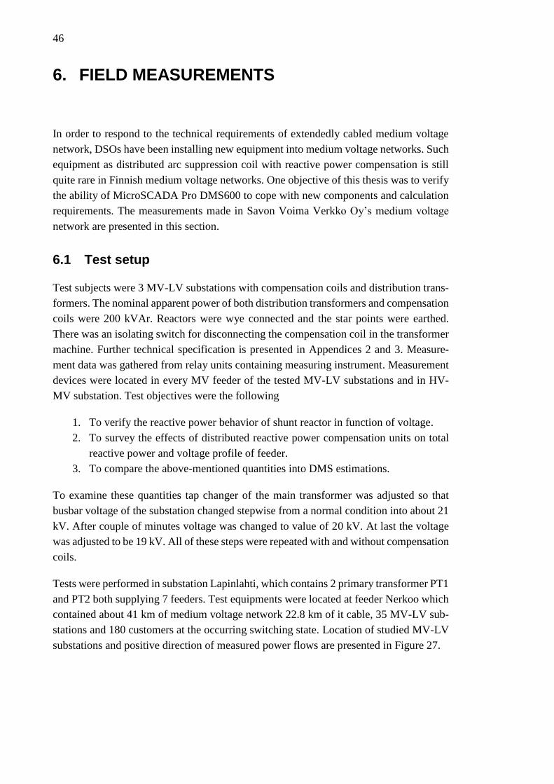
46
6. FIELD MEASUREMENTS
In order to respond to the technical requirements of extendedly cabled medium voltage
network, DSOs have been installing new equipment into medium voltage networks. Such
equipment as distributed arc suppression coil with reactive power compensation is still
quite rare in Finnish medium voltage networks. One objective of this thesis was to verify
the ability of MicroSCADA Pro DMS600 to cope with new components and calculation
requirements. The measurements made in Savon Voima Verkko Oy’s medium voltage
network are presented in this section.
6.1 Test setup
Test subjects were 3 MV-LV substations with compensation coils and distribution trans-
formers. The nominal apparent power of both distribution transformers and compensation
coils were 200 kVAr. Reactors were wye connected and the star points were earthed.
There was an isolating switch for disconnecting the compensation coil in the transformer
machine. Further technical specification is presented in Appendices 2 and 3. Measure-
ment data was gathered from relay units containing measuring instrument. Measurement
devices were located in every MV feeder of the tested MV-LV substations and in HV-
MV substation. Test objectives were the following
1. To verify the reactive power behavior of shunt reactor in function of voltage.
2. To survey the effects of distributed reactive power compensation units on total
reactive power and voltage profile of feeder.
3. To compare the above-mentioned quantities into DMS estimations.
To examine these quantities tap changer of the main transformer was adjusted so that
busbar voltage of the substation changed stepwise from a normal condition into about 21
kV. After couple of minutes voltage was changed to value of 20 kV. At last the voltage
was adjusted to be 19 kV. All of these steps were repeated with and without compensation
coils.
Tests were performed in substation Lapinlahti, which contains 2 primary transformer PT1
and PT2 both supplying 7 feeders. Test equipments were located at feeder Nerkoo which
contained about 41 km of medium voltage network 22.8 km of it cable, 35 MV-LV sub-
stations and 180 customers at the occurring switching state. Location of studied MV-LV
substations and positive direction of measured power flows are presented in Figure 27.
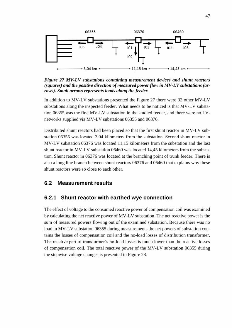
47
Figure 27 MV-LV substations containing measurement devices and shunt reactors
(squares) and the positive direction of measured power flow in MV-LV substations (ar-
rows). Small arrows represents loads along the feeder.
In addition to MV-LV substations presented the Figure 27 there were 32 other MV-LV
substations along the inspected feeder. What needs to be noticed is that MV-LV substa-
tion 06355 was the first MV-LV substation in the studied feeder, and there were no LV-
networks supplied via MV-LV substations 06355 and 06376.
Distributed shunt reactors had been placed so that the first shunt reactor in MV-LV sub-
station 06355 was located 3,04 kilometers from the substation. Second shunt reactor in
MV-LV substation 06376 was located 11,15 kilometers from the substation and the last
shunt reactor in MV-LV substation 06460 was located 14,45 kilometers from the substa-
tion. Shunt reactor in 06376 was located at the branching point of trunk feeder. There is
also a long line branch between shunt reactors 06376 and 06460 that explains why these
shunt reactors were so close to each other.
6.2 Measurement results
6.2.1 Shunt reactor with earthed wye connection
The effect of voltage to the consumed reactive power of compensation coil was examined
by calculating the net reactive power of MV-LV substation. The net reactive power is the
sum of measured powers flowing out of the examined substation. Because there was no
load in MV-LV substation 06355 during measurements the net powers of substation con-
tains the losses of compensation coil and the no-load losses of distribution transformer.
The reactive part of transformer’s no-load losses is much lower than the reactive losses
of compensation coil. The total reactive power of the MV-LV substation 06355 during
the stepwise voltage changes is presented in Figure 28.

48
Figure 28 Net reactive power and calculated average phase to phase voltage in MV-LV
substation 06355.
The phase to phase voltage in Figure 28 is calculated from the average value of the meas-
ured phase to earth voltages in MV-LV substation 06355. Each coil in wye connected
shunt reactor consumes reactive power proportional to the voltage between phase and the
star point of reactor. Therefore the total reactive power consumed by reactor can be cal-
culated with an equation (39) in which the system voltage is the main voltage calculated
from the average value of phase to earth voltages.
6.2.2 Effect of shunt reactors in load flow of feeder
Shunt reactors are used in medium voltage network to compensate the reactive power
generated by medium voltage network cables. Measurements were done to examine the
effects of distributed shunt reactors on medium voltage reactive power flow and current
capacity in stable and in varied voltage conditions.
In Figure 29 the supplied reactive power and the current of the studied feeder are pre-
sented while the distributed shunt reactors are disconnected one by one. The upright
dashed lines represent the moments when the shunt reactors were disconnected.
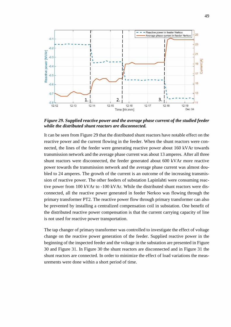
49
Figure 29. Supplied reactive power and the average phase current of the studied feeder
while the distributed shunt reactors are disconnected.
It can be seen from Figure 29 that the distributed shunt reactors have notable effect on the
reactive power and the current flowing in the feeder. When the shunt reactors were con-
nected, the lines of the feeder were generating reactive power about 160 kVAr towards
transmission network and the average phase current was about 13 amperes. After all three
shunt reactors were disconnected, the feeder generated about 600 kVAr more reactive
power towards the transmission network and the average phase current was almost dou-
bled to 24 amperes. The growth of the current is an outcome of the increasing transmis-
sion of reactive power. The other feeders of substation Lapinlahti were consuming reac-
tive power from 100 kVAr to -100 kVAr. While the distributed shunt reactors were dis-
connected, all the reactive power generated in feeder Nerkoo was flowing through the
primary transformer PT2. The reactive power flow through primary transformer can also
be prevented by installing a centralized compensation coil in substation. One benefit of
the distributed reactive power compensation is that the current carrying capacity of line
is not used for reactive power transportation.
The tap changer of primary transformer was controlled to investigate the effect of voltage
change on the reactive power generation of the feeder. Supplied reactive power in the
beginning of the inspected feeder and the voltage in the substation are presented in Figure
30 and Figure 31. In Figure 30 the shunt reactors are disconnected and in Figure 31 the
shunt reactors are connected. In order to minimize the effect of load variations the meas-
urements were done within a short period of time.

50
Figure 30. Reactive power and voltage in the beginning of feeder. Distributed shunt
reactors are disconnected.
Figure 31. Reactive power and voltage in the beginning of feeder. Distributed shunt
reactors are not connected.
It can be seen from figures that the variation in supplied reactive power is more dependent
on voltage in system where distributed shunt reactors are not connected. In case the shunt
reactors are connected there are no noticeable changes in reactive power while voltage is
varied. This is caused by the fact that the reactive power generated by cable is compen-
sated already in the distributed shunt reactors. If the shunt reactors are disconnected, the
reactive power generated along the feeder is transported to the beginning of feeder.

51
6.3 Comparison of measurements and DMS600 calculations
6.3.1 Model of shunt reactors
Tested equipment with an earth fault current compensation capability and a reactive
power compensation capability was modeled in MicroSCADA Pro DMS600 before the
measurements. The model of the equipment consisting of a distribution transformer and
a wye connected shunt reactor with earthed star point is presented in Figure 32.
Figure 32. The model of a MV-LV substation consisting of a distribution transformer
and a wye connected reactor with earthed star point.
Since there is no possibility in DMS600 to model a shunt reactor, a capacitor was coded
to DMS600. The nominal reactive power of the capacitor was set to be negative to repre-
sent the consumption of reactive power. In order to model the coil’s earth fault current
compensation capability an arc suppression coil was coded to the MV-LV substation.
The active power consumed in MV-LV substation 06355 includes the losses of the shunt
reactor and the losses of the distribution transformer. The LV-network of the transformer
was disconnected so the losses of the transformer were formed merely by the no-load
losses of the distribution transformer. The nominal losses of the shunt reactor are 7550
W and no-load losses of the distribution transformer are 405 W, so the losses are mainly
generated in the shunt reactor. In order to verify the accuracy of the modeled equipment,
calculated and measured reactive and active powers in case of different connection volt-
ages are presented in Figure 33 and in Figure 34.

52
Figure 33. The measured and calculated reactive power values in case of three different
voltages affecting over shunt reactor.
Figure 34. The measured and calculated active power values in case of three different
voltages affecting over shunt reactors
It can be seen from Figure 33 that the reactive power is accurately calculated in DMS. In
Figure 34 it is shown that the calculated active power remarkably differs from the meas-
ured active power. The differences between active powers is mainly due to the losses in
shunt reactor. In DMS the reactor is modeled with an ideal capacitor, and the losses of
the substation are constant no-load losses of the distribution transformer.
6.3.2 Effect of shunt reactors on voltages along feeder
In order to test the accuracy of state estimation, the measured voltages along the feeder
are compared to voltages that are calculated based on estimated loadings. Measured pow-
ers along the feeder and in the beginning of the feeder can be used in the DMS's load
estimation. Usually only measurements from the beginning of the feeder are used because
there are no measurements available from the MV-LV substations. Measured voltages are
0
50
100
150
200
20,9 20 18,8
kVA
r
Voltage [kV]
Q in DMS Measured Q
0
1
2
3
4
5
6
7
20,9 20 18,8
kW
Voltage [kV]
Measured P P in DMS

53
compared to calculated voltages in two different situation. In the first case the loads are
estimated based on the measured powers and the voltage in the beginning of feeder. In
second case also measured powers from 3 MV-LV substations along the feeder are used
in estimation. The measured voltages along the feeder are compared to calculated volt-
ages during different voltage levels in substation with and without distributed shunt reac-
tors. Results in case the shunt reactors were disconnected are presented in Figure 35.
Results in case shunt reactors were connected are presented in Figure 36. In both figures
the voltages of three MV-LV substation are presented in case of three voltage level. Clus-
tered column “DMS” represents estimated voltages in case only measured P, Q and V
values from substation were used. Clustered column “DMS2” represents calculated volt-
ages in case also measured powers from the MV-LV substations were used. The measured
powers from the MV-LV substations along the feeder that were used in estimation are
presented in Appendix 4. Measured and estimated voltages are presented in Appendix 5.
Estimation tests were done after the real measurements by adding the saved measurement
values in each step into DMS-database. The SQL-queries that were used in setting of
measurement values are presented in Appendices 6 and 7.
Figure 35. The measured and estimated voltages along inspected feeder in case of dif-
ferent tap changer positions. Shunt reactors are not connected.
18
18,5
19
19,5
20
20,5
21
6355 6376 6460 6355 6376 6460 6355 6376 6460
kV
MV-LV substation
DMS DMS2 Measured

54
Figure 36. The measured and estimated voltages along inspected feeder in case of dif-
ferent tap changer positions. Shunt reactors are connected.
Calculated voltages are higher than measured voltages in every measurement points. The
differences between measured and calculated voltages is in worse case about 200 V. The
use of power measurements along the feeder seem not to make the voltage calculation
more accurate in this system. The difference remains that big probably because of the
other distribution transformers along the line branches without measurements. Also the
fact that the load curves were in somewhat different state at the time the test was done
than at the time measurements were done makes some error to the test results. The effect
of load curves can be assumed small because there are no loads in inspected feeder that
would have large variations in consumption.
However there was no load between the HV-MV substation and the MV-LV substation
06355 so it is expected that the voltage of that line section would be accurately calculated.
In order to test the DMS’s calculation method, the voltage difference occurring in that
line section was also calculated with Matlab. The line section was modeled with one pi-
section and the receiving end voltage was calculated with the measured sending end volt-
age and current. The used Matlab-script is presented in Appendix 8. Line parameters used
in calculation are presented in Table 3.
Table 3. The parameters of the first line section.
Length [m] Resistance [Ω/km] Reactance [Ω/km] Susceptance [µS/km]
3040 0,125 0,110 94,20
The measured receiving end voltage and voltage calculated with Matlab and DMS are
presented in Figure 37. Only case that is above presented in Figure 35 is presented. Shunt
reactors are disconnected.
18
18,5
19
19,5
20
20,5
21
6355 6376 6460 6355 6376 6460 6355 6376 6460
kV
MV-LV substation
DMS DMS 2 Measured

55
Figure 37. Voltages in 06355. Measured, Matlab (pi-section) and DMS600
It can be seen in Figure 37 that the results of DMS and Matlab pi-section does not differ
from each other much. Therefore the differences between the measured and calculated
voltages are caused from the improper calculating parameters rather than improper cal-
culation method. The accuracy of voltage measure is ± 0,5 %, the accuracy of reactive
power measure is ± 3 %, accuracy of active power measure is ± 1 % and accuracy of
current measure is ± 5 % or 1 A [34]. The inaccuracies of measurement values explains
part of the differences. One possible reason for differences between calculated and meas-
ured voltages might be that the resistance of cable is bigger than resistance used in calcu-
lation because there are multiple medium voltage cables close to each other. If the cable
warm up it might cause the resistance of the cable to rise. On the basis of ohm’s law the
voltage drop is higher in lines with higher resistance.
6.4 Development needs to DMS600 based on measurements
As presented in Section 6.3.1 the model of shunt reactor used in pilot study models the
reactive power of wye connected shunt reactor with sufficient accuracy. However the
active power of shunt reactor is high and the reactor cannot be modeled as an ideal sink
of reactive power. Thereby the active losses of shunt reactors needs to be taken into ac-
count. In order to make the coding of Dyn11+YN transformer easier, an own component
for transformer is needed.
In Section 6.3.2 the measured and the calculated voltages were compared case of two
different DMS configuration. It seems that P and Q measurements in 3 MV-LV substa-
tions along the feeder did not make the estimation of voltages more accurate but the power
18,5
19
19,5
20
20,5
21
21,5
21,14 19,88 19,03
kV
Busbar voltage [kV]
DMS Matlab Measured

56
flow was divided more accurately between feeder branches. Differences between meas-
ured and calculated voltages are not, however, caused by false calculation but more likely
caused by inaccuracies in measurements.

57
7. PSCAD SIMULATIONS
In this section simulations are performed to examine the present DMS version's ability to
perform earth fault calculations in extensively cabled distribution network. Basically the
accuracy of commonly used conventional earth fault analysis is compared to a more com-
plex analysis method. Simulations are made with a simple network model consisting of
shunt reactors and one type of cable. The cable that is used in simulations is AHX-W240.
Line parameters are the same that have been used in pilot project of ABB Oy and Savon
Voima Verkko Oy. Line parameters are presented in Table 4. Susceptance b have been
calculated from the corresponding capacitive reactance values for DMS.
Table 4. AHX-W240 calculation parameters used in simulations
R [mΩ/m] Xi [mΩ/m] Xc [MΩ*m] b [µs/km]
Pos. sequence 0.139 0.116 10.6 94.340
Zero sequence 0.576 0.221 10.97 91.158
Centralized arc suppression coil is connected to a busbar via an earthing transformer
whose calculation parameters for each winding are presented in Table 5. Sn is the nominal
apparent power, Xl is the leakage resistance, P0 is the leakage resistance and Pk is the
copper losses of the transformer.
Table 5. The calculation parameters of the centralized coil's zero point transformer
U1/U2 Sn [kVA] Xl [pu] P0 [pu] Pk [pu]
6,83/6,83 300 0,078 0,0011 0,014
Distributed arc suppression coils are modeled as YN coupled coils. The calculation pa-
rameters of the shunt reactors are listed in Table 6. Un is the nominal voltage, Qn is the
nominal compensated reactive power, Ion is the nominal compensated earth fault current
and R/X is the resistance-reactance ratio of the coil.
Table 6. The calculation parameters of shunt reactor [Appendix 2]
Un [kV] Qn [kVAr] Ion [A] R/X [%]
20,5 200 16,9 2,5
In earth fault analysis of DMS only the zero sequence susceptance of the line presented
in Table 4 and the nominal compensation current of arc suppression coil presented in

58
Table 6 are used. The zero sequence capacitance is used in conventional earth fault anal-
ysis also in [1] p. 62. The calculation voltage in DMS’s earth fault analysis is 20 kV so
the tap changer in PSCAD model is adjusted to maintain voltage 20 kV in busbar during
every network configuration.
7.1 Effect of long cable in earth fault current calculations
In order to study the DMS’s ability to model earth faults in network consisting large
amount of cable, simulations were made in networks containing different amount of ca-
ble. Modeled network contains 5 feeders. 4 of the feeders consists of 5 km AHX-W240
cable. In this simulation case the length of one studied feeder was varied from 5 to 35 km.
There were no line branches in the studied feeder nor in the background network. Two
simulation cases were studied in every network configuration. In first case a solid earth
fault occurred in the beginning of the studied feeder and in second case a solid earth fault
occurred in the farthermost node of the studied feeder. It is not, however, possible to
define a fault point in DMS so only one situation case was calculated by DMS. In both
cases only the centralized coil was used to compensate the earth fault current. The induct-
ance of the centralized coil was adjusted to compensate 90 % of the earth fault in the
busbar by using equation (41). The compensation current 𝐼𝐿 of an arc suppression coil
was set to be 90 % of the earth fault current that flows to the ground in case an earth fault
occurred in the beginning of the studied feeder.
𝐿 =
𝑈𝑛
√3𝜔𝐼𝐿
(41)
In the first case the fault occurred in the beginning of the studied feeder. The fault current
in the fault place is presented in Figure 38. In figures Ifc is the capacitive part of the fault
current, Ifr is the resistive part of the fault current, Iftot is the total fault current,
Iftot_DMS is the total fault current calculated by DMS. Ifc2, Ifr2 and Iftot2 are the cor-
responding quantities in case the fault occurred in the end of the studied feeder. All sim-
ulation results are presented in detail in Appendix 9.

59
Figure 38. Fault current in fault place. Fault is in the beginning and in the end of the
studied feeder. The length of studied feeder is varied.
As expected, the differences between the results of PSCAD and DMS simulations are
bigger with longer lines. In case the studied feeder is 5 km long the earth fault current
calculated by DMS is about 2 amperes lower than the earth fault current calculated by
PSCAD. In case the studied feeder is 35 km long the difference between the results is
about 8 amperes. Since the difference becomes larger with longer lines, it can be deduced
that different line parameters are used in calculation in PSCAD and DMS. In PSCAD’s
calculation method both zero sequence and positive sequence parameters effect on the
earth fault current. As explained in Section 7, the zero sequence susceptance was set to
be the ground susceptance of the line in DMS. Other possible reason for differences is the
losses in earthing transformer and other parts of sequence networks. Due to the losses the
centralized coil does not produce the inductive current that it adjusted to produce based
on equation (41). However, it needs to be noticed that in DMS user can define the com-
pensated current for centralized coil. DMS’s calculation method does not take stand on
what inductance is needed to achieve that current.
It can also be seen that the resistive part of the fault current increases while the length of
the feeder increases. This is caused by the resistive losses of lines, earthing transformer
and arc suppression coil. The resistive part of earth fault current reaches maximum value
of 5.41 A in case the feeder is 35 km long and the earth fault occurs in the beginning of
the feeder. It can also be seen that the total fault current is about the same size inde-
pendently of the fault place. However the reactive part and resistive part of the fault cur-
rent are different in different fault places.
0
2
4
6
8
10
12
14
16
18
20
22
24
26
5 10 15 20 25 30 35
Ief
[A]
The length of studied feeder [km]Ifc Ifr Ifc2 Ifr2 Iftot Iftot_DMS Iftot2

60
In Figure 39 the neutral point displacement voltages are presented. In PSCAD simulation
the voltages are calculated from the sum of busbar voltages. In figure U0 is the neutral
point displacement voltage in case the fault occurs in the beginning of feeder and
U0_DMS is the neutral point displacement voltage calculated by DMS. Coefficient U02
is corresponding quantity in case the fault occurs in the end of studied feeder.
Figure 39. Neutral point displacement voltage. Fault is in the beginning and in the end
of studied feeder. The length of studied feeder is varied. Centralized arc suppression
coil is adjusted to keep compensation ratio in 90 % in case the fault occurs in the be-
ginning of feeder.
Results indicates that the neutral point displacement voltage calculated by DMS is close
to simulated, but the difference between results increases in case of longer lines. The
voltage changes while the length of feeder is increased probably due to the bigger effect
of series impedances.
The neutral point displacement voltage of this system is higher if the earth fault occurs in
the end of the feeder. In multiple papers it have been claimed that the zero sequence series
impedance causes the drop in neutral point displacement voltage if the fault occurs in the
end of long cable feeder. In this simulation model for example the zero sequence re-
sistance of cable is 0.576 Ω/km, which is very low compared to for example 2,52 Ω/km
used in Master of Science thesis of Sami Vehmasvaara [12].
7.2 Effect of distributed compensation in earth fault calcula-
tions
In order to study the DMS’s ability to model the earth fault situation in case of different
use cases of compensation coils, simulations were made with the same network model
used in previous section. The length of the studied feeder is in this simulation case 35 km
because this is, based on interviews, probably the longest cabled trunk line in Finnish
distribution networks. In this case a solid earth fault occurred in the beginning of the
11,45
11,5
11,55
11,6
11,65
11,7
5 10 15 20 25 30 35
U0
[kV
]
The length of studied feeder [km]
U0 U0_DMS U02

61
studied feeder. In first simulation case the centralized compensation coil was set to main-
tain constant compensation degree and the amount of 16,9 A shunt reactors in the system
was varied. In second simulation case the centralized compensation coil was not used but
the amount of distributed shunt reactors was varied. In both cases the placing of the dis-
tributed coils was started from the end of the feeder and those were located in a way that
each coil compensates the capacitive earth fault current that the cable around it generated.
First 6 coils were placed into the studied feeder. After that coils were placed also in feed-
ers in background feeders. Results of each simulation case is in detail presented in Ap-
pendix 9.
7.2.1 Combination of centralized and distributed compensation
Before the simulations the earth fault generated by inspected feeder was calculated by
DMS in order to solve how many distributed coils could be installed on that feeder with-
out the feeder to be overcompensated. The inspected feeder generates earth fault current
110,5 A so there could be maximum 110,5 A / 16,9 A = 6.5 local coils. Feeders in back-
ground network generates 15,8 A earth fault current, so those would be overcompensated
if coil was installed in those feeders. The inductance of the centralized coil is determined
by the earth fault current without any compensation. Earth fault current in case of solid
earth fault in the beginning of inspected feeder in case of an isolated neutral system is
180,25 A based on PSCAD model and 173,7 A based on DMS model. The inductance L
of centralized coil is calculated with equation (41), where 𝑈𝑛 is the nominal main voltage,
𝐼𝐿 is (180,25 A)*0,9-(n*16,9 A) in PSCAD and (173,7 A)*0,9-(n*16,9 A) in DMS. N is
the number of distributed coils in network.
The effect of distributed coils on fault current and neutral point displacement voltages
based on PSCAD simulations and DMS calculations are presented in Figure 40, and in
Figure 41.

62
Figure 40. Earth fault current in fault point. Centralized coil is adjusted to keep the
compensation degree in 90 % while the amount of distributed coils is varied.
In Figure 40 it can be seen that based on PSCAD simulations the earth fault current de-
creases while the amount of distributed coils is increased even though the centralized coil
is adjusted to keep the compensation rate in a constant value. This is probably due to the
smaller effect of system’s series reactances when the amount of distributed coils is in-
creased. Also the resistive current component degreases while coils are located in the
faulted feeder because of this phenomena. Also the fact that the amount of earth fault
current compensated by distributed coil is not always the nominal 16,9 A, effects on the
differences between results of PSCAD and DMS. It needs to be noticed that in DMS user
can define the compensated current for centralized coil. DMS’s calculation method does
not take stand on what inductance is needed to achieve that current. However, as expected,
the earth fault coefficients go closer to the coefficients calculated based on assumptions
while the amount of coils is increased.
Figure 41. Neutral point displacement voltage. Centralized coil is adjusted to keep the
compensation degree in 90 % while the amount of distributed coils is varied.
0
5
10
15
20
25
0 1 2 3 4 5 6 6+1 6+1+1 6+1+1+1
Ief
[A]
The amount of distributed coils
Ifc Ifr Iftot Iftot_DMS
11,45
11,5
11,55
11,6
11,65
0 1 2 3 4 5 6 6+1 6+1+1 6+1+1+1
U0
[kV
]
The amount of distributed coils
U0 U0_DMS

63
In Figure 41 it is shown that the increased amount of distributed coils decreases the neu-
tral point displacement voltage. This is probably due to the smaller effect of system’s
series reactances when the amount of distributed coils is increased. Based on conventional
earth fault analysis the neutral point displacement voltage is constant while the compen-
sation degree is constant. The difference between results in this system is in worse case
about 100 V and the minimum difference is about 80 V.
7.2.2 Distributed compensation
In second case only distributed compensation coils are used. The earth fault currents and
neutral point displacement voltages are simulated in system where the amount of distrib-
uted coils is varied. First the studied feeder is almost completely compensated with the
local coils and then one compensation coil is placed also in every feeder in background
network. The results of simulations are presented in Figure 42 and in Figure 43.
Figure 42. Earth fault current in fault place. Only distributed coils are used.
It can be seen in Figure 42 that the use of distributed coils decreases the amount of earth
fault current. There is a small difference between results of PSCAD simulation and DMS,
and the difference degreases while use of distributed coils increases. The difference be-
tween the results in worse case is 6,55 A and the minimum difference is 2,7 A. The dif-
ference between results degreases probably due to the degreasing effect of series imped-
ances while the amount of distributed coils increases.
0
20
40
60
80
100
120
140
160
180
Ief
[A]
The amount of distributed coils
Ifc Ifr Iftot Iftot_DMS

64
It can also be seen that the amount of resistive earth fault current starts to grow when the
coils are installed in background network. In this case probably the total amount of resis-
tive losses in zero sequence network begins to grow.
Figure 43. Neutral point displacement voltage. Only distributed coils are used.
Figure 43 shows that there is some difference in the results of the neutral point displace-
ment voltages if only few distributed coils are used. The difference between the results is
in worse case about 320 V. Not until the network is almost totally compensated a differ-
ence remains between the results. In that case also the PSCAD simulation model acts as
conventional earth fault analysis assumes.
7.3 Development needs to DMS600 based on simulations
The earth fault results calculated with the PSCAD simulation model and with the DMS
model have some differences. First of all the zero sequence capacitance was used in con-
ventional earth fault analysis, that caused smaller earth fault currents than PSCAD model.
Other differences between the results of PSCAD and DMS are caused by simplifications.
These simplifications can be made when the earth fault related calculations are made in
networks consisting multiple short cable feeders. As it have been presented in previous
simulations the calculation results are not accurate in a network consisting long cable
feeder. If the results remarkably differs from the values of the real system, false calcula-
tion results might cause larger touch voltages and difficulties in detecting earth faults.
However there are inaccuracies and simplifications in the PSCAD model that is used in
previous simulations. Especially the zero sequence impedance of cable is not known ex-
actly. Therefore, the actual earth fault behavior of cables is not known precisely.
The biggest differences in the calculation results appear in a system with a long cable
feeder where the distributed compensation coils are not used. The results would be more
11,45
11,55
11,65
11,75
11,85
11,95
U0
[kV
]
The amount of distributed coils
U0 U0_DMS

65
accurate if the positive sequence impedance and also the series impedance of zero se-
quence impedance was taken into account. Also the impedances of the earthing trans-
former and the resistance of the distributed coils needs to be taken into account to get
more accurate results. It might also be useful for DMS user if the resistive and reactive
parts of the earth fault current was presented in addition to the total current. In systems
consisting of longer cables, whose zero sequence resistance is larger than the resistance
used in the previous simulation model, the earth fault quantities might have different re-
sults in different fault places. In that case DMS should provide a feature for analyzing
earth faults in different fault places.

66
8. INTERVIEWS
One objective of this thesis was to find the need for improvements in the aspect of me-
dium voltage network cabling. Representatives of 4 distribution system operators were
interviewed in order to discuss the problems that large scale medium voltage network
cabling causes and to find the development needs to MicroSCADA Pro DMS600 to fa-
cilitate their work. In this chapter the DSOs’ cabling objectives, compensation strategies
and development ideas are presented. Also the feasibility of Volt-VAr Control for Finnish
customers is discussed in this section.
8.1 Cabling objectives
In recent years increased long electricity distribution interruptions caused by storms and
major weather events had the legislators and Energy Authority to consider tightening and
amendment to Electricity Market Act and authority requirements. New Electricity Market
Act was given in 9th August 2013 and it came into effect on 1st September 2013. The aim
of the law is to improve the reliability of electricity distribution and to reduce the long
interruptions caused by major weather events. According to the new law distribution net-
work must be planned, built and maintained so that fault in the distribution networks
caused by a storm or snow load doesn’t cause an interruption for customers with maxi-
mum duration of six hours per occurrence in the town plan area and 36 hours per occur-
rence in other area. 100 % of DSO’s customers must meet the requirements set in article
at latest by 31st December 2028 including holiday houses. [28]
Cabling is one way to improve the reliability of distribution because cable is protected
from storms and snow loads. In this section the interviewed DSO’s cabling objectives and
practices are presented.
8.1.1 Elenia Oy
Elenia Oy serves 415 000 customers in its operational area in Tavastia Proper, Päijänne-
Tavastia, Tampere region, South Ostrobothnia and Northern Ostrobothnia. [35] Elenia
Oy’s distribution network consists of 23 000 km of medium voltage line and 40 000 km
of low voltage line. [36] Already in 2009 Elenia Oy made a decision that all re-build lines
will be constructed underground cable. [35] The cabling goal is to have cabling rate of 70
% in both medium voltage and in low voltage networks. At the moment the cabling rate
of medium voltage network is 20 % and the cabling rate of low voltage network is 40 %.
To achieve the cabling goal 900 km of medium voltage cable and 1000 km of low voltage
cable is installed yearly at least in next years. [36]

67
Already before the new reliability requirements Elenia Oy studied the fault points saved
in DMS to determine the cabling requirements for achieving proper reliability of delivery.
The cabling goal 70 % + 70 % was set based on this study. The cabling is not, however,
the only way to improve the reliability of delivery. For example automation is in big role
since lots of overhead line remains in network. [36]
The main focus of cabling is at the moment in urban area and in rural area trunk cables
since it have been proved to be the most cost efficient solution in low loaded rural area
networks. Tomi Hakala have studied the issue in his Master of Science thesis, “Prioriti-
zation principles for the reinvestment plan of low loaded parts of the rural medium voltage
network” [37]. The cabling of trunk cables in rural area network have proved to be a good
solution also in practice since Elenia Oy have already cabled a few 30-40 km long trunk
cables between rural area substations. Even though faults occur in line branches, those
are disconnected from the trunk line and the delivery of the whole feeder is interrupted
only a short time. During major storm the cabled trunk line is energized and the faulted
branches can be fixed and restored one by one. [36]
8.1.2 Koillis-Satakunnan Sähkö Oy
Koillis-Satakunnan Sähkö Oy provides electricity distribution services in South Ostro-
bothnia, central Finland and in Tampere region. [38] Distribution network of Koillis-Sa-
takunnan Sähkö Oy consists of 1600 km of medium voltage line and 2300 km of low
voltage line. At the moment cabling rate is 3,7 % in medium voltage network and 26 %
in low voltage network. [39]
Koillis-Satakunnan Sähkö Oy aims to have 100 % cabling rate in urban network areas to
meet the reliability requirements. The total cabling of urban areas networks requires how-
ever only about 55 km of additional medium voltage network cabling. Cabling pace in
medium network will be about 20 km per year in next two years, but after the urban are
have been cabled, it will take a long time to achieve cabling rate of 10 % in medium
voltage network. In a low voltage network cabling rate will be increased by 3 percentage
unit every year until the cabling rate of 65 – 70 % is achieved. [39]
The main strategy of Koillis-Satakunnan Sähkö Oy for achieving the reliability require-
ments in rural area network is to move overhead lines close to road. This have been proved
to be an efficient solution for avoiding trees falling to lines and for facilitating the clearing
of the fault. Cabling of rural area medium voltage networks is not considered to be a good
solution because of the following issues:
Expenses in relation to supplied power
Slow localization and reparation of a cable fault
Lack of backup connections

68
Soil conditions and waterways
The re-build low voltage network is however decided to build with an underground cable
because the low voltage underground cable is usually even more profitable than overhead
line. [39]
8.1.3 Leppäkosken Sähkö Oy
Leppäkosken Sähkö Oy operates distribution network in area of Ikaalinen, Jämijärvi,
Kihniö, Parkano, Hämeenkyrö and Ylöjärvi. Distribution network consists of 1500 km of
medium voltage line and 2800 km of low voltage line. At the moment 9,6 % of medium
voltage network and 39 % of low voltage network is cabled. In order to enhance the reli-
ability of delivery Leppäkosken Sähkö Oy pursuits a cabling rate of 40 % in the medium
voltage network and cabling rate of 60 % in the low voltage network until year 2028.
These goals are achieved by a cabling pace of 34 km per year in the medium voltage
network and 45 km per year in the low voltage network. Leppäkosken Sähkö Oy have
relatively short feeders compared to rural area networks. When the cabling goals are
achieved the longest cabled feeders will consist of 20-30 km cable. The longest rural area
feeder consists of 54 km of line, but it will not be cabled. [40]
At the moment 42 % of customers in urban area network and 13 % of customers in rural
area network are connected in network that complies with the requirements of maximum
interruption time of 6 h in urban area and 36 h in rural area. Underground cabling is not
an automatic way to reconstruct an old network. Cable is used in places that it is cost
efficient. Among cabling the other ways to improve the reliability of delivery are listed
below.
Maintaining of fault clearance organization
Backup connections
Moving overhead lines close to road
Effective clearing of overhead line routes
There have never been an interruption of delivery in distribution network of Leppäkosken
Sähkö Oy that have lasted over 36 h, which is why the effective fault clearance organiza-
tion is in big role in their strategy. [40]
8.1.4 Savon Voima Verkko Oy
Savon Voima Verkko Oy operates distribution network in eastern Finland. Distribution
network consists of about 25 500 km lines and electricity is delivered for over 113 000
consumption points. [41] At the moment there are 11 202 km of medium voltage line and
13 991,5 km of low voltage line in distribution network of Savon Voima Verkko Oy. 5,9
% of the medium voltage network and 27 % of the low voltage network is cabled. The
69
goal is to cable 25 – 30 % of medium voltage network. In 2020 17 % of the medium
voltage network will be cabled. Distribution network of Savon Voima Verkko Oy is
mainly rural area network. There are 225 meters of lines per one customer in their distri-
bution network, which is significantly more than in urban area networks having only
about 20 meters of line per one customer. This is why it is not profitable to invest more
in cable.
There will be long cabled feeders in rural area networks. The longest cabled feeder at the
moment is the feeder Nerkoo, where the measurements of this thesis were done. The trunk
line of Nerkoo is about 14,6 km long and there are lots of line branches.
8.2 Compensation strategies
Increased medium voltage network cabling give rise to earth fault current and reactive
power generated in lines. In this section compensation strategies and future plans among
these problems of interviewed utilities are presented.
8.2.1 Earth fault current
At the moment networks are used both unearthed and compensated, but the future trend
in all interviewed distribution system operators is to have at least centralized arc suppres-
sion coil in every substation. Leppäkosken Sähkö Oy have recently installed a centralized
compensation coil to all substations. Elenia Oy, Koillis-Satakunnan Sähkö Oy and Savon
Voima Verkko Oy will install centralized compensation coil in all substations in near
future. Also distributed compensation is already being used in parallel with centralized
coil. The combination of centralized and distributed compensation coils is the future so-
lution for the challenges of cable network within all interviewed DSOs’ distribution net-
works. The benefits of this solution are listed below. [40] [39] [36] [42]
Investing in distributed coils postpones the investing in larger centralized coil. In
very large cabled network earth fault current might even be so large that central-
ized coil with sufficient capacity is not even available. [40] [36] [42]
Distributed coils decreases the transportation of earth fault current and thus the
resistive component of earth fault current. [40] [36] [42]
Without centralized coil the earth fault current remains too high because the dis-
tributed coils cannot be dimensioned optimally for all switching states. [36]
Without centralized compensation coil resonance circuit might appear that causes
unwanted relay tripping. [36]
The increased use of distributed arc suppression coils is somewhat new approach to com-
pensation of earth fault current and hereby causes new concerns to be taken care of in
70
planning and operation of distribution network. The strategy of distributed coil dimen-
sioning in Elenia Oy is that 80 % of earth fault current generated in line section between
remote controlled switches is compensated locally, and rest of the earth fault current is
compensated with centralized coil. This strategy is set to prevent the overcompensation
of individual feeder in any switching state made by remote controlled switches. There
remains however possibility of overcompensation if the state of manually operated
switches is changed. [36] Overcompensation of feeders is the main concern also in other
interviewed utilities. Leppäkosken Sähkö Oy and Savon Voima Verkko Oy are also will-
ing to optimally dimension and place the distributed coil from the aspect of the earth fault
current’s resistive part. [40]
8.2.2 Reactive power
Increased cabling of medium voltage network increases the reactive power generated in
low loaded network. All of the interviewed distribution system operators envisage that
the increased cabling raises new requirements for the planning and for the operation of
network. The main reason for adjusting reactive power is the reactive power window of
Fingrid Oy, because expenses rise quickly if the window is exceeded. Especially if the
reactive power of every HV-MV substation is started to monitor separately in the begin-
ning of year 2016, the DSOs need to pay more attention to the reactive power consump-
tion and generation. Since the generated reactive power might exceed the reactive power
window during summer nights already in networks consisting of mainly overhead lines,
the situation will be more severe in networks that consist of mainly cable.
At present time all of the interviewed utilities have capacitors in some of the HV-MV
substations and in switching stations to support the voltage of weak overhead lines [36],
to raise voltage during replacement of HV-MV substation [40] or to prevent the reactive
power consumption from exceeding the consumption side of the reactive power window.
[39]. While the amount of medium voltage cable increases the need for capacitors prob-
ably decreases in many situations and the demand for shunt reactor increases. Elenia Oy
and Savon Voima Verkko have been testing a few distributed shunt reactors along long
cable feeders. Representative of Elenia Oy told that the heating of distributed shunt reac-
tors might cause problems and needs to be taken into consideration. The reactive power
compensation strategy of Elenia Oy is that shunt reactors are installed in HV-MV substa-
tions and in switching stations because the centralized compensation is the most cost ef-
ficient way to compensate reactive power. The strategy is a result of Master science thesis
of Sami Vehmasvaara “Compensation strategies in cabled rural networks”. [36]
Leppäkosken Sähkö Oy have not desided the final compensation strategy, but they see
that it might be more cost effective in their network to compensate reactive power with
distributed coils. Leppäkosken Sähkö Oy will probably use coils with compensation
capabilities of both earth fault current and reactive power. [40] Also Savon Voima Verkko

71
Oy will use the disttibuted compensation method. The cabling rate of Koillis-Satakunnan
Sähkö Oy will be so low that they unlikely invest in shunt reactors. [39]
In addition to shunt reactors and capacitors distribution system operators aim to minimize
the transportation of reactive power by charging customers for noticeable consumption
or generation of reactive power. Leppäkosken Sähkö Oy and Elenia Oy charges for the
use of reactive power but Koillis-Satakunnan Sähkö Oy charges for both generation and
consumption of reactive power. The reactive power charge have turned out to be an
effective way to encourage customers to instal own compensation devices. [40] [39] [36]
Also distributed energy resources affect in the reactive power flow and in the voltage
stability of distribution network. Interviewed DSOs have generation in their network.
Koillis-Satakunnan Sähkö Oy has a few hydroelectric power plants of which reactive
power generation is being controlled from the control room via SCADA. The reactive
power generation of power plants are being controlled to keep the reactive power flow of
the system inside the reactive power window. The power plants are however connected
to HV-MV substation busbar or there are own feeders without consumpiton for the power
plants. Above-mentioned arrangements make the protection analysis and the controlling
of voltages in customer supply points easier. [39] Elenia Oy have no planning strategy
for distributed generation. Representatives of Elenia Oy envision that the microgeneration
connected to low voltage networks is distributed widely and the amount of power plants
connected to medium voltage network will not increase since small power plants are not
profitable. [36]
8.3 Customer requirements and ideas
In this section the customers’ development ideas and needs are presented. The require-
ments are divided into earth fault current and reactive power –related sections and also
the overheating of cable –related concern is introduced.
8.3.1 Earth fault current compensation
As it have been previously mentioned, the use of distributed arc suppression coils is going
to increase and the replacement of centralized arc suppression coils is in many cases com-
pulsory since the capacity of old coils is not sufficient. Customers requires tools for plan-
ning the optimal location and sizing of arc suppression coils. Also checks and notices
made by DMS are required to help the operator in the risk analysis of different network
configurations.

72
8.3.1.1 Calculation of earth fault current caused by multiple net-
work plans
Since the capacities of the presently installed centralized arc suppression coils are not at
the moment large enough to compensate the earth fault current of cabled networks, the
coils needs to be replaced with bigger ones. [40] Also the strengthening of earthing is
planned by the calculations of network information system. [36] Multiple network plans
are performed in the same HV-MV substation area and all of them are affecting on the
earth fault current of the network. A procedure now for deciding the correct time for coil
replace is to separately execute earth fault calculation for each plan and then by hand
calculate the total earth fault current in each phase of the cabling process. Network infor-
mation system should provide a possibility for calculating an earth fault calculation for
multiple network plans in the same time. [37] [36] Furthermore NIS could provide the
calculation results in each phase of planned network construction process.
8.3.1.2 Calculations to prevent overcompensation of feeder
The placing and sizing of distributed arc suppression coils should be done in a way that
an individual feeder stays under compensated in every switching state. This should be
done to ensure the correct functioning of conventional earth fault relays. [40] [39] [36]
[42] For example in Elenia Oy this requirement is being implemented so that arc suppres-
sion coils are being dimensioned to compensate 80 % of the earth fault current generated
in the line between each remote controlled switches. The compensation degree of lines is
being calculated by hand by dividing the inductive current of local coil with the generated
earth fault current of particular line section. [36] Network information system should pro-
vide a compensation degree of each feeder in an earth fault results list. This information
could also be visualized by colors in network window, which would ease the checking of
compensation degree in multiple different network configurations. [36] [40]
8.3.1.3 Support for admittance protection
Some of the interviewed DSOs are willing to invest in a new technology in the area of
network protection. For example Savon Voima Verkko Oy requires that the admittance
protection would be supported in DMS. In present DMS version only older relay types
are supported. DMS should provide a possibility to document relay configuration of the
admittance relay and the configuration data should be used to check the performance of
relay configuration. [42]
8.3.1.4 More detailed earth fault analysis
As have been presented in Section 2.5.2.1 the use of distributed arc suppression coils
decreases the transportation of earth fault current and hence the resistive part of it. Also
the neutral point displacement voltage and residual current seen by relay remains some-
what independent on fault location if the distributed coils are placed between optimal
intervals. In Elenia Oy the more detailed protection analysis is not being done by the
network planners by NIS, but in Leppäkosken Sähkö Oy MicroSCADA Pro DMS600 is

73
being used also for earth fault relay configuration planning. [36] [40] Network infor-
mation system should provide more detailed information about earth faults. For example
resistive and reactive part of residual current and neutral point displacement voltage in
case of different fault locations are needed for exact relay configuration and distributed
coil placing [40].
8.3.1.5 Notices for operator
Compared to network consisting of mainly overhead lines, more attention needs to be
paid in earth fault current issues in cabled networks. In extendedly cabled network the
maximum earth fault current generated in feeders varies significantly during switching
state changes. In addition, in systems where distributed compensation is used, new issues
needs to be taken into consideration.
The increase of earth fault current raises a possibility that the capacity of an automatically
controlled centralized coil is not large enough to compensate the earth fault current of a
large network. Centralized coils have a controller which knows the current state of coil’s
reactance. This information is delivered to SCADA and an alarm is added to an alarm list
if needed. However the alarm is not being noticed until the coil’s state has reached the
alarming value. This is why the capacity of compensation coil should be taken into con-
sideration in switching planning mode and warn the switching planner if the maximum
limit of compensation coil will be reached. In addition to the notices in switching planning
mode, the operator should be warned if the earth fault current is larger than the maximum
compensation capacity of the centralized coil in state monitoring mode. This way all in-
formation would be available in DMS even if the state of the compensation controller is
not available in SCADA. [40] [36]
The use of distributed compensation coils needs to be taken into account also in operation
of distribution network. Even though the location and size of distributed coils have been
tried to be planned in a way that the feeder would not be overcompensated in any switch-
ing state, it is not always possible in a network consisting of multiple switching compo-
nents. For example in Elenia Oy local compensation is sized to compensate 80 % of the
earth fault current generated in lines between two remote-controlled switches. There are
however manually-controlled disconnectors in network that may cause the overcompen-
sation of the feeder. DMS should provide information about this kind of situation. Infor-
mation should be available when switching sequence is planned and also in a state mon-
itoring mode. With the help of information in switching planning the switching planner
would be aware of the situation and may decide whether more complex switching se-
quence is necessary to avoid the overcompensation. In case the abnormal switching state
lasts only a short amount of time the overcompensation does not necessarily cause any
actions. In case that abnormal switching state will last a long time, further switching is
needed. If the overcompensation situation is left in the network for example during major
storm, it is important that the switching state will later be fixed to normal. Therefore DMS

74
should provide for example coloring mode that highlights the feeders that are overcom-
pensated. The same visualization could be used that is already described in Section
8.3.1.2. [36]
8.3.2 Reactive power
Extended use of medium voltage cable increases the reactive power generated in distri-
bution network. In order to effectively plan the reactive power compensation and to han-
dle the voltage and reactive power balance, adequate component models and load flow
calculations in NIS and DMS are required. What also needs to be taken into consideration
in network operation is that the reactive current generated by network might significantly
vary if the switching state is changed. In this section requirements for NIS and DMS are
presented to support the decision making of DSOs.
8.3.2.1 Modeling of components
The installation of a shunt reactor effects on the load flow of a network and needs to be
therefore properly modeled. In addition to static reactors also automatically controlled
reactors might be used in the near future [36]. Also a component consisting of distribution
transformer and a star connected reactor with an earthable star point will be used in near
future in the distribution networks of many DSOs. The latter one needs to be modeled
with one component in order to have proper component reports and to avoid unnecessary
network coding. What needs to be taken into consideration in the model of this component
is that there is a possibility to disconnect the star point and earth. In this case the compo-
nent operates as a shunt reactor but it does not compensate any earth fault current. The
star point might be disconnected in case that cabling process have not been proceeded so
far that earth fault current compensation is needed, but the required component is installed
in advance [40].
8.3.2.2 Calculation of reactive power caused by multiple network
plans
As it have already been explained in case of an earth fault current in Section 8.3.1.1,
multiple plans in the MV network of the same HV-MV substation effects also on the
reactive power generation of the whole network. A possibility to calculate the reactive
power flow of multiple network plans is important because the reactive power flowing
through primary transformer causes losses and might exceed the Ingrid’s reactive power
window. If the effect of multiple plans was calculated, the need for centralized shunt re-
actor would be easily evaluated in advance. However the generation of reactive power
highly depends on the current loading situation, so there should be possibility to calculate
the reactive power flow in case of different loadings. [36]

75
8.3.2.3 Notices for operator
In a network consisting of only overhead lines the major concern in network switching
planning have been the voltage drop along the feeders. In case of an extendedly cabled
network the voltage rise might be a bigger problem. Also the amount of reactive power
transferred through the primary transformer needs to be observed more closely. DMS
should provide information to avoid these problems. At the moment in some utilities the
Ingrid’s power window is monitored in SCADA. If the reactive power limits were saved
to DMS, it would be possible to warn the operator for the exceeding of reactive power
window already during switching planning. [36]
8.3.3 Overheating of cable
The cooling time constant of a cable is larger than the cooling time constant of an over-
head line, which means that cables cool down more slowly than overhead lines. This
phenomena arouses a concern that the cable could heat up during the fault isolating pro-
cess if multiple test switching are done with a fast sequence before the fault point is iso-
lated. Representatives of PKS Sähkönsiirto Oy proposed that DMS should inform the
network operator if there is a possibility of cable overheating. [43]
Also the concern aroused among interviewed representatives that the load current might
reach the maximum allowed current in abnormal switching states. Measured currents
should be used and an operator should be informed if the maximum loading current of
line is reached. [42]
8.4 Feasibility of Volt-VAr Control for Finnish customers
One objective of this thesis was to discuss if the Volt-VAr Control feature of Mi-
croSCADA Pro DMS600 is a considerable solution for the reactive power problems
caused by the increased use of MV cable. The conclusions on this section are mainly
based on interviews. VVC includes two different operation modes as presented in Section
5.3.4. In power factor correction mode capacitor banks, voltage regulators, on load tap
changers and the outputs of power plants are being controlled to maintain the reactive
power transportation at minimum state. Conservation voltage reduction can be used to
minimize the capacity expansions of distribution system. Power factor correction mode
might help the DSOs in the problems caused by the increasing reactive power generation.
Interviewed DSOs have few capacitors in their networks and the capacitors are being used
only in exceptional situation. On the contrary the use of compensation coils will increase
due to the MV cables and the reactive power window. Among interviewed DSOs Koillis-
Satakunnan Sähkö Oy and Elenia Oy prefer the centralized coil to distributed coils. Other
interviewed DSOs will probably use distributed compensation coils. In the aspect of VVC
it is important to remember that for example Dyn11+YN transformers’ reactive output

76
cannot be adjusted. Those cannot neither be disconnected because there is a normal dis-
tribution transformer also behind the transformer’s disconnector. However, the central-
ized shunt reactors can be disconnected. If the use of passive centralized coils will in-
crease, those could be controlled by VVC feature.
There are no voltage regulators in interviewed DSO’s networks and tap changers cannot
usually be used for reactive power control because it effects on the voltage of the whole
network. Usually voltage is close to the minimum allowed level in some point of the
network. Therefore, in addition to shunt reactors and capacitors, other possible control
variables in the distribution networks of interviewed DSOs are the reactive power outputs
of power plants. A small scale distributed generation is not considered a problem among
interviewed DSOs but the reactive power outputs of larger generators in medium voltage
networks are already controlled among some of the DSOs. The medium voltage power
plants in the networks of interviewed DSOs are supplying power directly to HV-MV sub-
stations or those are connected to substation via own feeders. This is why the control of
reactive power output is not that urgent compared to control in networks where consump-
tion and generation are located in the same feeder. However, reactive power output is
being controlled to maintain the reactive power flow between HV and MV networks in
sustainable level. The use of VVC feature would facilitate the work of operators espe-
cially in systems containing multiple power plants.
Probably the biggest benefit of VVC would be achieved if the actions of VVC feature
could be modelled already when a feeder for a new power plants is being planned. In that
case there would not necessarily be need for a network that strong and expenses could be
minimized. Therefore, NIS should provide a planning tools in which the active voltage
control mode is taken into account. Development needs of NIS in the aspect of active
voltage control methods have been further investigated in the Doctor of Science Thesis
of Anna Kulmala: Active Voltage Control in Distribution Networks Including Distributed
Energy Resources [22].

77
9. RESULTS
9.1 Developed solutions and methods
During the measurements, simulations and interviews multiple development needs for
NIS and DMS were brought out. In this chapter the needed methods to achieve the re-
quirements are proposed. At first the new devices and the methods to correctly model the
devices’ electrical phenomena are presented. After that the solutions to improve the cal-
culation methods of present earth fault analysis feature are presented. At last the methods
to develop a more accurate earth fault analysis feature, additional notices and visualiza-
tions are presented. Also the outline of the feature for multiple network plan calculations
is presented.
9.1.1 New devices
In order to correctly model the earth fault behavior and the load flow of system, the com-
ponents need to be correctly documented and modelled in DMS’s network model. Until
now the reactive power compensation have been implemented mainly with capacitors.
Therefore there have not been a need for modeling reactors in DMS. Also the components
used in earth fault current compensation have not been modelled in detail in DMS. In
order to enhance earth fault calculation results, more detailed model of earth fault related
components needs to be gathered.
9.1.1.1 Shunt reactor
Shunt reactor is used to compensate the reactive power that lines generate during low load
situation. Shunt reactors can be star or delta coupled. The reactive power consumption of
reactor depends on the reactance of coils and on the voltage over the coils. Even though
the coupling of reactor effects on the power consumption as presented in Section 3.2.2, it
is convenient in DMS to calculate the reactive power based on the nominal power and
voltage of reactor as presented in equation (40). Based on measurements presented in
Section 6.3.1 and interviews presented in Section 8.2, the active power losses of shunt
reactors needs to be modelled also.
The connection voltage can be taken by the result of state estimation calculations but the
nominal values of reactor needs to be gathered during network coding. It is already pos-
sible in present DMS version to code a shunt reactor in DMS network model, but the
nominal values are not gathered. The values needed to model a shunt reactor are the fol-
lowing:
Nominal voltage
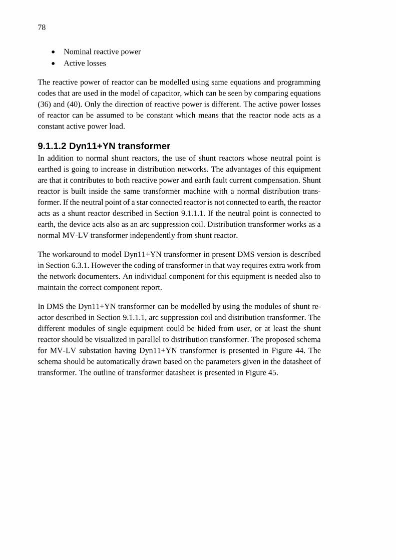
78
Nominal reactive power
Active losses
The reactive power of reactor can be modelled using same equations and programming
codes that are used in the model of capacitor, which can be seen by comparing equations
(36) and (40). Only the direction of reactive power is different. The active power losses
of reactor can be assumed to be constant which means that the reactor node acts as a
constant active power load.
9.1.1.2 Dyn11+YN transformer
In addition to normal shunt reactors, the use of shunt reactors whose neutral point is
earthed is going to increase in distribution networks. The advantages of this equipment
are that it contributes to both reactive power and earth fault current compensation. Shunt
reactor is built inside the same transformer machine with a normal distribution trans-
former. If the neutral point of a star connected reactor is not connected to earth, the reactor
acts as a shunt reactor described in Section 9.1.1.1. If the neutral point is connected to
earth, the device acts also as an arc suppression coil. Distribution transformer works as a
normal MV-LV transformer independently from shunt reactor.
The workaround to model Dyn11+YN transformer in present DMS version is described
in Section 6.3.1. However the coding of transformer in that way requires extra work from
the network documenters. An individual component for this equipment is needed also to
maintain the correct component report.
In DMS the Dyn11+YN transformer can be modelled by using the modules of shunt re-
actor described in Section 9.1.1.1, arc suppression coil and distribution transformer. The
different modules of single equipment could be hided from user, or at least the shunt
reactor should be visualized in parallel to distribution transformer. The proposed schema
for MV-LV substation having Dyn11+YN transformer is presented in Figure 44. The
schema should be automatically drawn based on the parameters given in the datasheet of
transformer. The outline of transformer datasheet is presented in Figure 45.

79
Figure 44. Proposed schema for MV-LV substation consisting of two MV disconnectors
J01, J02, distribution transformer and shunt reactor. M1 is the transformer discon-
nector, R1 is the disconnector for reactor and R2 is the disconnector between Y coupled
reactor and earth.
Figure 45. Transformer datasheet with a possibility to document shunt reactor
Shunt reactor is drawn in the substation schema if “Shunt reactor” is selected in the trans-
former’s datasheet. The disconnector R2 between neutral point and earth shown in Figure
44 is generated if “Disc.” is selected from datasheet. If “solid” is selected, the discon-
nector is not drawn. R/X value is the ratio of reactor’s resistance and reactance, which
can be used in earth fault current calculations described in Section 9.1.6. If the discon-
nector R2 is open the shunt reactor consumes reactive power but does not effect on earth

80
fault behavior of the system. If the disconnector R2 is closed, the shunt reactor consumes
reactive power but also acts as an arc suppression coil during an earth fault.
9.1.1.3 Variable shunt reactor
The use of variable shunt reactors will not remarkably increase among interviewed DSOs,
but the representative of Elenia said in interview that VSRs might be one possible solution
to maintain reactive power balance in their network. If the prices of VSRs become down
also other DSOs might begin to use these devices. VSR is automatically controlled by
controller to keep the reactive power consumption at constant value almost independently
from the voltage level. VSRs voltage dependency is discussed more in Section 3.2.3.
In DMS VSR could be modelled using the same data that was presented in Section 9.1.1.1.
In addition to data used in the passive shunt reactor, also minimum and maximum reactive
power limits needs to be documented. Also the configuration of VSR should be docu-
mented to predict the behavior of VSR during simulations and switching planning.
9.1.2 Earth fault calculation in case of mixed compensation
During simulations it was noticed that the present version of DMS600 cannot handle all
of the needed earth fault current calculations of system consisting of both centralized and
distributed compensation coils. At present the earth fault calculation list consist of a total
earth fault current, a current generated by feeder and a residual current seen by relay in
case the earth fault occurs in the inspected feeder. In the present DMS version the total
earth fault current in fault place is calculated correctly, but the residual currents of faulted
and healthy feeders are calculated in a wrong way .
The earth fault theory of conventional earth fault analysis in network consisting of cen-
tralized and distributed coils is presented in Section 2.3. The residual current of faulted
feeder should be calculated with equation (14), which can be derived from Figure 8.
Based on the same figure, the equation for residual current of healthy feeder should be
calculated with equation (42). 𝐿𝐹𝑑 represents the inductance of coils in studied feeder and
L is the total inductance of the network.
𝐼𝑟 =
√1 + (𝑅𝐿(3𝜔𝐶𝐹𝑑 −1
𝜔𝐿𝐹𝑑))2
√(𝑅𝑓 + 𝑅𝐿)2 + (𝑅𝑓𝑅𝐿(3𝜔𝐶 −1
𝜔𝐿))2
𝑈
√3 (42)
Applying these corrections the present conventional earth calculation feature would offer
good approximation of important earth fault quantities in system where centralized and
distributed compensation coils are used at the same time.

81
9.1.3 Visualization to prevent overcompensation of feeder
In order to support the network planner and operators in handling of distributed arc sup-
pression coils, NIS and DMS should provide information from the compensation rate of
feeders. As presented in Section 8.2.1 DSOs plan the location of distributed coils in a way
that the individual feeder does not become overcompensated in any normal switching
state. DMS should provide information in earth fault calculation list and in network view
by colors. A proposed visualization concept for compensation degree is presented in Fig-
ure 46. In figure A the compensation rate is below 100 %. In figure B the feeder is over-
compensated because only a short line section and a second distributed coil are connected
to the feeder.
Figure 46. Visualization concept for the compensation degree of feeders. A: There is
only one coil in the feeder. Feeder generates more earth fault current than local coil
compensates -> K < 100 %. B: There are two coils in the short feeder -> K > 100 %.
With this visualization concept network planner could easily check that the feeder will
not be overcompensated in any possible switching state. This visualization would also
help network operator to prevent the overcompensation during switching operations and
to correct the switching state for example after major storm.
In addition to visualization, the compensation capacity generated by distributed coils and
centralized coils should be calculated in the earth fault calculation list. This way the com-
pensation degree of feeders would be available in earth fault report and the capacity of
centralized compensation coil would be easily monitored. The proposed earth fault result
list with above mentioned corrections is presented in Figure 47.

82
Figure 47. Proposed earth fault result list with an additional information. Figure is for
demonstration use only. Results are not valid.
In case of a system presented in figure mixed compensation is used. The maximum com-
pensation current of centralized compensation coil is 180 A, and the sum of nominal cur-
rents of distributed coils is 264,5 A. The centralized coil is set to keep compensation
degree in 95 %. Earth fault currents are calculated in case of the present compensation
equipment and in case of isolated system. From these results also a used compensation
capacity is calculated. The total used compensation capacity is calculated with equation
100 % * (116 A / 264,5 A) = 43,8 % and the used capacity of centralized coil is calculated
with equation 100 % * ((116 A – 84,5 A) / 180 A) = 17,5 %. Also a column “DISTR.
COMP. DEGREE” have been added into the list of feeder’s results. It can be seen that
for example 80 % of earth fault current generated by feeder Cleveland is compensated
with distributed coils.
9.1.4 Notices and events
One main function of DMS is to give notices for user to prevent the operations that might
cause for example unwanted relay tripping or danger. Both earth fault current and reactive
power generation might change noticeably when the switching state of cabled network is
changed. Already in present version of DMS multiple checks are done during switching
planning mode. For example breaking capacity of circuit breakers is checked. The addi-
tional check that should be done during switching planning are the following:

83
Capacity of centralized compensation coil
Overcompensation of feeder
Exceeding of reactive power window
Capacity of centralized compensation coil needs to be checked every time the amount of
generated earth fault current changes. If the total earth fault current exceeds the maximum
current of coil, a warning should be given. Also the distributed coils needs to be taken
into account.
During switching planning overcompensation of feeders should be checked and noticed
every time switching is done. Check should work in the same way than the visualization
described in Section 9.1.3.
Exceeding of the reactive power window might cause expenses rather quickly. DMS
should check if the reactive power transferred to transmission network is larger than a
defined limit. The generated reactive power depends on the current loading situation and
is thus difficult to accurately forecast. However, the forecasted loads and conductor data
can be used to estimate the generated reactive power during the hour the switching is
planned to be executed. In order to enable the described notice, reactive power limits for
each connection points needs to be defined for example in the datasheet of feeding points
in HV-MV substations.
9.1.5 Calculation of multiple plans
DSOs have multiple ongoing network plans, for example cabling projects, in the area of
same HV-MV substation. Because the cabling significantly changes the reactive power
and earth fault current generation, DSOs need to invest in shunt reactors and arc suppres-
sion coils. The need and size of investments depend on the total reactive power or earth
fault current of HV-MV substation. It is possible in present DMS600 NE version to exe-
cute load flow and earth fault analysis only for one plan at the time. It should be possible
to select network plans from the area of same HV-MV substation whose mutual reactive
power and earth fault results would be calculated at the same time. The proposed calcu-
lation result list is presented in Figure 48.

84
Figure 48. The example of the combined calculation results of multiple network plans
From the results presented in Figure 48 network planner can track the growth of an earth
fault current, the amount of compensation capacity, the amount of reactive power and the
power losses in network in different phases of network construction process. Also other
information that is calculated already in present DMS version should be calculated for
multiple plans.
9.1.6 Advanced earth fault protection analysis
It have been stated previously in Sections 2.4 and 7 that the conventional earth fault anal-
ysis with multiple assumptions might not be accurate enough to analyze the earth fault
phenomena in networks consisting long cables or multiple distributed arc suppression
coils. Many assumptions and simplifications are also made in DMS’s earth fault analysis.
The major assumptions that should be corrected are the following:
Arc suppression coils are ideal
Earthing transformers are not taken into account
Equivalent circuit consists of only zero sequence capacitance, coil inductance and
fault resistance
Due to these assumptions the zero sequence voltage is the same in the fault place and in
HV-MV substations despite the fault place. Also the location of distributed coils does not
effect on the earth fault behavior of the system. In order to make the earth fault analysis
more accurate more information needs to be used in calculations. Arc suppression coils
are usually connected to the tertiary winding of auxiliary transformer in substation. It

85
should be possible to document the correct connection methods to DMS. This way the
zero sequence impedance of the transformer could be used in earth fault analysis. Second
option is to add the zero sequence impedance of whole earthing equipment in the
datasheet of arc suppression coil. In latter case it should be taken into account that the
zero sequence impedance of coils is multiplied by three in equivalent circuit, but the im-
pedance of transformer is not multiplied. In addition to impedances of earthing equip-
ment, more conductor data needs to be used. Already in present DMS version as well as
positive sequence resistance and reactance also zero sequence resistance and zero se-
quence reactance are saved into database.
After the required data is saved into database, more accurate earth fault analysis feature
can be applied. In advanced calculation method the sequence networks needs to be created
and the zero sequence impedance of earthing transformer needs to be taken into account
in calculation of neutral point displacement voltage. The theory of method is presented in
Section 2.6. The main steps of analysis method in the aspect of DMS is presented in
following:
1. User select the fault point and a fault impedance to be analyzed
2. Create the positive, negative and zero sequence impedances seen from the fault
point as described in Section 2.6.
3. Calculate and show the fault current in fault point (equation (21)), residual cur-
rents of all feeders (equation (22)) and neutral point displacement voltage (equa-
tion (23)).
With the results of this analysis method DSOs can more accurately investigate the effect
of long cable and the amount of arc suppression coils on relay configurations. Still inac-
curacy remains in the zero sequence impedance of lines if user have not been saved the
correct impedances into database. There are some equations that could be used in the
calculation of zero sequence impedances, for example one presented in Section 2.4.1. One
possibility is that DMS generates an approximation of zero sequence impedance for lines
using equation (15). The earthing impedance data can be saved into DMS database so that
data could be used in calculation of zero sequence impedance. However, the most effec-
tive method to solve the zero sequence impedance is to measure it [44]. If measurement
values are used, user needs to document an own conductor type for each measured line
section because the value of zero sequence impedance depends on installation type and
earthing of sheath.

86
10. CONCLUSIONS
This thesis studied the development needs of ABB MicroSCADA Pro products portfo-
lio’s network information system and distribution management system from the aspect of
medium voltage network cabling. Objectives of the thesis were to gather information
about the problems that medium voltage cabling causes for DSOs and to examine the
DMS’s present ability to support users in these issues. Four DSOs were interviewed and
measurements and simulations were made to find the development needs to software.
Also the feasibility of Volt-VAr Control feature for Finnish DSOs was discussed.
Volt-VAr Control feature could facilitate network operators work because then operators
would not need to control the reactive power output of power plants, capacitors and reac-
tors to avoid the costs that are caused by reactive power transportation. However, there
are not much capacitors nor power plants in interviewed DSOs’ medium voltage net-
works. In addition, most of the DSOs are going to install shunt reactors that are not con-
trollable. The biggest benefit of VVC would be achieved if the actions of VVC feature
could be modelled already when a feeder for a new power plants is being planned. In that
case there would not necessarily be need for a network that strong and expenses could be
minimized. Therefore, NIS should provide a planning tools in which the active voltage
control mode is taken into account.
Earth fault analysis and reactive power generation in case of a long rural area cable were
the main issues that have been studied in this thesis. Most of the interviewed DSOs will
increase the use of distributed earth fault current compensation and reactive power com-
pensation devices. Combination of centralized and distributed arc suppression coils will
be increasingly used because that way the phenomena caused by the series impedance of
a long cable will be minimized. Other advantage of mixed compensation is that DSOs
don’t necessarily need to invest in very large centralized arc suppression coils. Because
cables generate reactive power significantly more than overhead lines, also reactive
power is being compensated to prevent losses and to prevent the exceeding of Fingrid’s
reactive power window. Some of the interviewed DSOs will use centralized shunt reac-
tors and some of them will use distributed shunt reactors. Distributed shut reactors are
usually easier to install and those prevent the voltage from rising along a long feeder.
DSOs require more accurate earth fault calculation results, support in both planning and
handling of distributed arc suppression coils, accurate modeling of shunt reactors and arc
suppression coils, possibility to handle the calculation results of multiple network plans
and notices for operators to easier handle the reactive power and the capacity of central-
ized arc suppression coil during network operation. Also a feature for managing over-
heating of cable is proposed because cable cools down much slower compared to an over-
head line.

87
Earth fault analysis method used in present DMS version could be improved in order to
better fulfill the requirements needed in analysis of extensively cabled network. In the
present DMS version earth fault calculations are based on conventional earth fault analy-
sis, which contains certain assumptions. Equivalent circuit that is used in earth fault anal-
ysis consists of zero sequence capacitance of network, inductance of compensation coils
and fault resistance. In a system consisting of a long cable also the zero sequence series
impedance of lines and both the positive and negative sequence impedances of lines need
to be taken into consideration. In a system consisting of multiple distributed coils also the
total impedances of coils and earthing transformers need to be taken into account to ac-
curately calculate the earth fault currents and neutral point displacement voltages.
In the present DMS version it is possible to use the measurement values of current, volt-
age, reactive power and active power to estimate the load flow in network. DMS’s ability
to estimate voltages along feeder was tested in distribution network of Savon Voima
Verkko Oy. Powers, currents and voltages were measured from the beginning of the
feeder and from the three MV-LV substations along the feeder. Measured and estimated
voltages were compared in case of two different DMS configuration. In the first case only
busbar voltage and powers measured in the beginning of the feeder were used in the esti-
mation. In the second case also the measured powers from the MV-LV substations along
the feeder were used. It seems that estimated voltages are somewhat higher than measured
voltages. In the inspected system the use of measurements along the feeder did not make
the voltage calculation much more accurate, but the loading between line branches were
more accurately adjusted to match the measurements. The differences between the meas-
ured and calculated voltages are probably caused by the line branches, the inaccuracies
of measurements and inadequate calculation parameters such as line resistance. The volt-
age drop was also studied with Matlab and same results were obtained.
After the development needs were gathered, solutions and methods were developed to
meet the new requirements. Models for new devices such as shunt reactors and
Dyn11+YN transformers are presented. Visualization for feeders’ compensation degree
is proposed. Requirements for notices and events that would help the user maintaining
compensation degree and reactive power generation in acceptable limits are presented.
Requirements for calculation of multiple network plans from the aspect of reactive power
and earth fault current are presented. Finally the needed changes to software for develop-
ing a more detailed earth fault analysis feature was presented.
Several changes to DMS600’s calculation functions are needed and more data needs to
be saved into database. The additional data can be used for the more accurate modeling
of shunt reactors and arc suppression coils during normal operating conditions and during
earth faults.

88
REFERENCES
[1] E. Lakervi and E. J. Holmes, Electricity distribution network design, IEE Power
Series 21, 2nd edition ed., Peter Peregrinus Ltd, 1995, p. 325.
[2] S. Hänninen, Single phase earth faults in high impedance grounded networks,
Characteristics, indication and location., Technical Research Centre of Finland
VTT, Otamedia, 2001, p. 78p. + app 61p.
[3] A. Guldbrand, Earth Faults in Extensive Cable Networks, Licentiate Thesis, Lund
University, Department of Measurement Technology and industrial Electrical
Engineering, 2009, p. 116 [121].
[4] A. Guldbrand, System earthing, Lund University, Industrial Electrical
Engineering and Automation, 2006, p. 12.
[5] E. Lakervi and J. Partanen, Sähkönjakelutekniikka, 3. ed., Otatieto / Gaudeamus
Helsinki University Press Oy Yliopistokustannus, HYY Yhtymä, 2008, p. 295.
[6] Finnish standards association SFS, SFS 6001 + A1 + A2 High-voltage electrical
installations, SESKO ry.
[7] E. Määttä, Earth fault protection of compensated rural area cabled medium
voltage networks, Master of Science Thesis, University of Vaasa, Faculty of
Technology, Electrical Engineering, 2014, p. 133.
[8] A. Wahlroos, J. Altonen and A. O. D. Automation, Compensated networks and
admittance based earth fault protection, 2011, p. 18.
[9] A. Wahlroos, J. Altonen, T. Hakola and T. Kemppainen, Practical application and
performance of novel admittance based earth-fault protection in compensated
MV-networks, Frankfurt: CIRED, 21 th International Conference on Electricity
Distribution, 2011, p. 4.
[10] Esa Virtanen, ABB Oy, Transformers, "Maaseutuverkkojen kaapelointi ja
loistehokysymykset," in Sähkön laadun hallinta -asiantuntijaseminaari, Luosto,
9.-13.2.2015, Luosto, 2015.

89
[11] H.-M. Pekkala, Challenges in extensive cabling of the rural area networks and
protection in mixed networks, Master of Science Thesis, Tampere University of
Technology, 2010, p. 130.
[12] S. Vehmasvaara, Compensation strategies in cabled rural networks, Master of
Science Thesis, Tampere University of Technology, 2013, p. 97.
[13] J. Jaakkola and K. Kauhaniemi, Factors Affecting the Earth Fault Current in
Large-Scale Rural Medium Voltage Cable Network, Stockholm: CIRED, 22 nd
International Conference on Electricity Distribution, 2013, p. 4.
[14] G. Brännman, Analysmodell för impedansjordat system med lokal
kompensering, University Of Trollhättan/Uddevalla, Department of Technology,
2003, p. 52.
[15] J. Elovaara and L. Haarla, Sähköverkot II, Gaudeamus Helsinki University
Press/Otatieto, 2011, p. 551.
[16] J. Elovaara ja L. Haarla, Sähköverkot 1, Järjestelmätekniikka ja sähköverkon
laskenta, Tallinna Raamatutrükikoda 2011: Gaudeamus Helsinki University
Press / Otatieto, 2011, p. 520.
[17] S. Repo, Sähkönsiirtoverkon jännitestabiilisuusmarginaalin approksimointi,
Tampere: Tampereen Teknillinen Korkeakoulu, 2000, p. 64.
[18] Fingrid Oyj, Kantaverkkosopimus 2012-2015, Fingrid Oyj, 2011, p. 16.
[19] Fingrid Oyj, Liite 4 Loissähkön sovellusohje, Fingrid Oyj, 2011, p. 5.
[20] Fingrid Oyj, "Uusi kantaverkkosopimus ohjaa loissähköön käyttöä," Fingrid,
Kantaverkko ja käyttövarmuus, 3/2014, p. 32, 25 11 2014.
[21] Fingrid Oyj, Tariffirakenne-esitys ja palautteet neuvottelukunta. Power point
slides, 2014.
[22] A. Kulmala, Active Voltage Control in Distribution Networks Including
Distributed Energy Resources, Doctor of Science Thesis, Tampere University of
Technology, 2014, p. 71.
[23] Areva T&D, "Shunt reactors in power systems, Tech News," [Online]. Available:
https://www.scribd.com/doc/60460850/Shunt-Reactor. [Accessed 19 2 2015].

90
[24] ABB Oy, "VarPro STATCOM, System designed by PLABB, Power point
slides," 2014.
[25] ABB Oy, "ABB Oy, STATCOM - SVC Light," ABB Oy, [Online]. Available:
http://new.abb.com/facts/statcom. [Accessed 15 5 2015].
[26] Trench, "Variable Shunt Reactors for Reactive Power Compensation," [Online].
Available: http://www.trenchgroup.com/en/Products-Solutions/Coil-
Products/Variable-Shunt-Reactors/node_727. [Accessed 20 2 2015].
[27] ABB Oy, "MicroSCADA Pro DMS600 4.4 FP1 System Administrator," 2014.
[Online]. Available:
https://library.e.abb.com/public/42da663268a9e60cc1257d6500426e56/DMS60
0_System%20Administration_757321_ENb.pdf?filename=DMS600_System%
20Administration_757321_ENb.pdf. [Accessed 7 5 2015].
[28] K. Kinnunen, Development of network information and distribution management
systems from the aspects reporting requirements, Tampere University of
Technology, 2014, p. 90.
[29] P. Järventausta, Feeder Fault Management in Medium Voltage Electricity
Distribution Networks, Tampere: Tampere University of Technology, 1995, p.
264.
[30] P. Verho, Configuration Management of Medium Voltage Electricity
Distribution Network, Manuscript 2009 ed., 2009, p. 126.
[31] ABB Oy, DMS600 Calculations. Calculation: Methods, Equations and Results,
p. 24.
[32] M. Kärenlampi, Interviewee, [Interview]. 11 2014.
[33] ABB Oy, Volt-var Optimization - A Case Study. Santee Cooper, 2014.
[34] ABB Oy, Remote I/O, RIO600 Product Guide, Product version 1.5, 2014.
[35] Elenia Oy, "Elenia Oy website," [Online]. Available: www.elenia.fi. [Accessed
24 3 2015].
[36] T. Lähdeaho, Interviewee, Interview at Elenia Oy. [Interview]. 13 3 2015.

91
[37] T. Hakala, Priorisation prinsiples for the reinvestment plan of low loaded parts of
the rural medium voltage network, Master of Science Thesis, T. U. o. technology,
Ed., Tampere University of Technology, 2013, p. 76.
[38] Koillis-Satakunnan Sähkö Oy, "Koillis-Satakunnan Sähkö Oy website,"
[Online]. Available: http://www.ksat.fi/fi/etusivu/sahkosopimuksen_tilaus.
[Accessed 24 3 2015].
[39] M. Pouttu and A. Ahonen, Interviewees, Interview at Koillis Satakunnan Sähkö
Oy. [Interview]. 9 3 2015.
[40] T. Salonen and M. Marttila, Interviewees, Inteview at Leppäkösken Sähkö Oy.
[Interview]. 4 3 2015.
[41] Savon Voima Oyj, "Savon voima homepage," [Online]. Available:
http://www.savonvoima.fi/Yritysesittely/Konserni/Sivut/konserni.aspx.
[Accessed 24 4 2015].
[42] T. Kiiski, J. Antikainen and M. Pirskanen, Interviewees, Savon Voima Verkko Oy
interview. [Interview]. 29 4 2015.
[43] M. Karhinen, Interviewee, PKS Sähkönsiirto Oy meeting. [Interview]. 17 12
2014.
[44] J. Altonen, Email message, 2015.


APPENDIX 1: QUESTIONNAIRE

APPENDIX 2: THE DATASHEET OF A DYN11+YN TRANS-
FORMER


APPENDIX 3: THE DIMENSIONAL DRAWING OF A TRANS-
FORMER
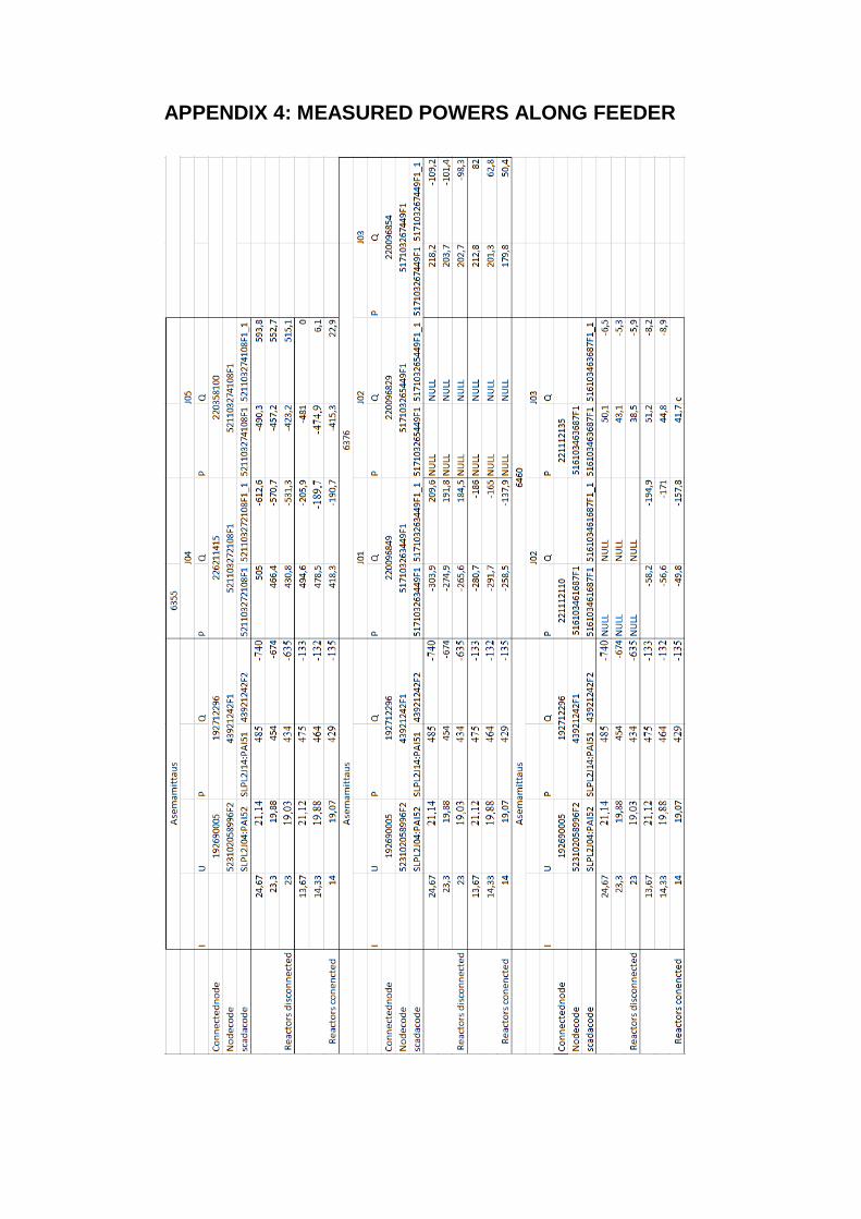
APPENDIX 4: MEASURED POWERS ALONG FEEDER

APPENDIX 5: MEASURED AND ESTIMATED VOLTAGES
Table 7. Comparison of measured and estimated voltages along the feeder. Shunt re-
actors are disconnected. P, Q and BB voltage are corresponding quantities in the be-
ginning of the feeder. Current is the current in the beginning of the feeder. Other pow-
ers used in load estimation are presented in Appendix 4.
P [kW] 485 454 434
Q [kVAr] -740 -674 -635
BB volt-
age [kV]
21,14 19,88 19,03
Fdr. volt-
age [kV]
Meas
ured
DMS DMS
2
Meas
ured
DMS DMS
2
Meas-
ured
DMS DMS
2
06355 20.89 21,14 21,14 19,66 19,88 19,88 18,78 19,03 19,03
06376 20.96 21,14 21,15 19,71 19,88 19,88 18,85 19,03 19,03
06460 20.96 21,14 21,14 19,72 19,87 19,87 18,83 19,03 19,03
Current
[A]
24.67 24,1 24,9 23.67 23,2 24,0 23.00 22,7 23,5

Table 8. Comparison of measured and estimated voltages along the feeder. Shunt re-
actors are connected. P, Q and BB voltage are corresponding quantities in the begin-
ning of the feeder. Current is the current in the beginning of the feeder. Other powers
used in load estimation are presented in Appendix 4.
P [kW] 475 464 429
Q [kVAr] -133 -132 -135
Voltage
[kV]
21,12 19.88 19.07
Fdr. volt-
age [kV]
Meas. DMS DMS
2
Meas. DMS DMS
2
Meas. DMS DMS
2
06355 20.88 21,11 21,11 19,58 19,87 19,87 18,84 19,06 19,06
06376 20.92 21,09 21,10 19,62 19,85 19,85 18,87 19,04 19,06
06460 20.92 21,09 21,09 19,62 19,85 19,85 18,87 19,03 19,06
Current.
[A]
13.67 13,4 13,8 14.33 14,1 14,9 14 14,6 13,2

APPENDIX 6: SQL QUERY FOR MEASUREVALUES
--Muristimet irti verkosta Update [SVV_OPERA_TESTI].[dbo].SwitchingComponent set StateE = '0', StateA = '0', StateB = '0', StateC = '0' WHERE (Switch LIKE '06460J01S1') OR (Switch LIKE '06355J01S1') OR (Switch LIKE '06376J01S1') --Step 1:jannite 21 kV --Asemasuureet Update [SVV_OPERA_TESTI].[dbo].measurevalues set value = 21.14 where scadacode like 'SLPL2J04:PAI52' --Kiskojan-nite Update [SVV_OPERA_TESTI].[dbo].measurevalues --Nerkoo patoteho set value = '485' where scadacode like 'SLPL2J14:PAI51' Update [SVV_OPERA_TESTI].[dbo].measurevalues --Nerkoo loisteho set value = '-740' where scadacode like '43921242F2' --Step 2: Jannite 20 kV --Asemasuureet Update [SVV_OPERA_TESTI].[dbo].measurevalues set value = '19.88' where scadacode like 'SLPL2J04:PAI52' --Kiskojan-nite Update [SVV_OPERA_TESTI].[dbo].measurevalues --Nerkoo patoteho set value = '454' where scadacode like 'SLPL2J14:PAI51' Update [SVV_OPERA_TESTI].[dbo].measurevalues --Nerkoo loisteho set value = '-674' where scadacode like '43921242F2' --Step 3: Jannite 19 kV --Asemasuureet Update [SVV_OPERA_TESTI].[dbo].measurevalues set value = '19.03' where scadacode like 'SLPL2J04:PAI52' --Kiskojan-nite Update [SVV_OPERA_TESTI].[dbo].measurevalues --Nerkoo patoteho set value = '434' where scadacode like 'SLPL2J14:PAI51' Update [SVV_OPERA_TESTI].[dbo].measurevalues --Nerkoo loisteho set value = '-635' where scadacode like '43921242F2' --Muristimet Kiinni verkossa Update [SVV_OPERA_TESTI].[dbo].SwitchingComponent set StateE = '1',

StateA = '1', StateB = '1', StateC = '1' WHERE (Switch LIKE '06460J01S1') OR (Switch LIKE '06355J01S1') OR (Switch LIKE '06376J01S1') --Step 1:jannite 21 kV --Asemasuureet Update [SVV_OPERA_TESTI].[dbo].measurevalues set value = '21.12' where scadacode like 'SLPL2J04:PAI52' --Kiskojan-nite Update [SVV_OPERA_TESTI].[dbo].measurevalues --Nerkoo patoteho set value = '475' where scadacode like 'SLPL2J14:PAI51' Update [SVV_OPERA_TESTI].[dbo].measurevalues --Nerkoo loisteho set value = '-133' where scadacode like '43921242F2' --Step 2: Jannite 20 kV --Asemasuureet Update [SVV_OPERA_TESTI].[dbo].measurevalues set value = '19.88' where scadacode like 'SLPL2J04:PAI52' --Kiskojan-nite Update [SVV_OPERA_TESTI].[dbo].measurevalues --Nerkoo patoteho set value = '464' where scadacode like 'SLPL2J14:PAI51' Update [SVV_OPERA_TESTI].[dbo].measurevalues --Nerkoo loisteho set value = '-132' where scadacode like '43921242F2' --Step 3: Jannite 19 kV --Asemasuureet Update [SVV_OPERA_TESTI].[dbo].measurevalues set value = '19.07' where scadacode like 'SLPL2J04:PAI52' --Kiskojan-nite Update [SVV_OPERA_TESTI].[dbo].measurevalues --Nerkoo patoteho set value = '429' where scadacode like 'SLPL2J14:PAI51' Update [SVV_OPERA_TESTI].[dbo].measurevalues --Nerkoo loisteho set value = '-135' where scadacode like '43921242F2'
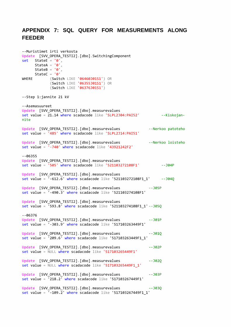
APPENDIX 7: SQL QUERY FOR MEASUREMENTS ALONG
FEEDER
--Muristimet irti verkosta Update [SVV_OPERA_TESTI2].[dbo].SwitchingComponent set StateE = '0', StateA = '0', StateB = '0', StateC = '0' WHERE (Switch LIKE '06460J01S1') OR (Switch LIKE '06355J01S1') OR (Switch LIKE '06376J01S1') --Step 1:jannite 21 kV --Asemasuureet Update [SVV_OPERA_TESTI2].[dbo].measurevalues set value = 21.14 where scadacode like 'SLPL2J04:PAI52' --Kiskojan-nite Update [SVV_OPERA_TESTI2].[dbo].measurevalues --Nerkoo patoteho set value = '485' where scadacode like 'SLPL2J14:PAI51' Update [SVV_OPERA_TESTI2].[dbo].measurevalues --Nerkoo loisteho set value = '-740' where scadacode like '43921242F2' --06355 Update [SVV_OPERA_TESTI2].[dbo].measurevalues set value = '505' where scadacode like '521103272108F1' --J04P Update [SVV_OPERA_TESTI2].[dbo].measurevalues set value = '-612.6' where scadacode like '521103272108F1_1' --J04Q Update [SVV_OPERA_TESTI2].[dbo].measurevalues --J05P set value = '-490.3' where scadacode like '521103274108F1' Update [SVV_OPERA_TESTI2].[dbo].measurevalues set value = '593.8' where scadacode like '521103274108F1_1' --J05Q --06376 Update [SVV_OPERA_TESTI2].[dbo].measurevalues --J01P set value = '-303.9' where scadacode like '517103263449F1' Update [SVV_OPERA_TESTI2].[dbo].measurevalues --J01Q set value = '209.6' where scadacode like '517103263449F1_1' Update [SVV_OPERA_TESTI2].[dbo].measurevalues --J02P set value = NULL where scadacode like '517103265449F1' Update [SVV_OPERA_TESTI2].[dbo].measurevalues --J02Q set value = NULL where scadacode like '517103265449F1_1' Update [SVV_OPERA_TESTI2].[dbo].measurevalues --J03P set value = '218.2' where scadacode like '517103267449F1' Update [SVV_OPERA_TESTI2].[dbo].measurevalues --J03Q set value = '-109.2' where scadacode like '517103267449F1_1'

--06460 Update [SVV_OPERA_TESTI2].[dbo].measurevalues --J02P set value = NULL where scadacode like '516103461687F1' Update [SVV_OPERA_TESTI2].[dbo].measurevalues --J02Q set value = NULL where scadacode like '516103461687F1_1' Update [SVV_OPERA_TESTI2].[dbo].measurevalues --J03P set value = '50.1' where scadacode like '516103463687F1' Update [SVV_OPERA_TESTI2].[dbo].measurevalues --J03Q set value = '-6.5' where scadacode like '516103463687F1_1' --Step 2: Jannite 20 kV --Asemasuureet Update [SVV_OPERA_TESTI2].[dbo].measurevalues set value = '19.88' where scadacode like 'SLPL2J04:PAI52' --Kiskojan-nite Update [SVV_OPERA_TESTI2].[dbo].measurevalues --Nerkoo patoteho set value = '454' where scadacode like 'SLPL2J14:PAI51' Update [SVV_OPERA_TESTI2].[dbo].measurevalues --Nerkoo loisteho set value = '-674' where scadacode like '43921242F2' --06355 Update [SVV_OPERA_TESTI2].[dbo].measurevalues set value = '466.4' where scadacode like '521103272108F1' --J04P Update [SVV_OPERA_TESTI2].[dbo].measurevalues set value = '-570.7' where scadacode like '521103272108F1_1' --J04Q Update [SVV_OPERA_TESTI2].[dbo].measurevalues --J05P set value = '-457.2' where scadacode like '521103274108F1' Update [SVV_OPERA_TESTI2].[dbo].measurevalues set value = '552.7' where scadacode like '521103274108F1_1' --J05Q --06376 Update [SVV_OPERA_TESTI2].[dbo].measurevalues --J01P set value = '-274.9' where scadacode like '517103263449F1' Update [SVV_OPERA_TESTI2].[dbo].measurevalues --J01Q set value = '191.8' where scadacode like '517103263449F1_1' Update [SVV_OPERA_TESTI2].[dbo].measurevalues --J02P set value = NULL where scadacode like '517103265449F1' Update [SVV_OPERA_TESTI2].[dbo].measurevalues --J02Q set value = NULL where scadacode like '517103265449F1_1' Update [SVV_OPERA_TESTI2].[dbo].measurevalues --J03P set value = '203.7' where scadacode like '517103267449F1' Update [SVV_OPERA_TESTI2].[dbo].measurevalues --J03Q set value = '-101.4' where scadacode like '517103267449F1_1'

--06460 Update [SVV_OPERA_TESTI2].[dbo].measurevalues --J02P set value = NULL where scadacode like '516103461687F1' Update [SVV_OPERA_TESTI2].[dbo].measurevalues --J02Q set value = NULL where scadacode like '516103461687F1_1' Update [SVV_OPERA_TESTI2].[dbo].measurevalues --J03P set value = '43.1' where scadacode like '516103463687F1' Update [SVV_OPERA_TESTI2].[dbo].measurevalues --J03Q set value = '-5.3' where scadacode like '516103463687F1_1' --Step 3: Jannite 19 kV --Asemasuureet Update [SVV_OPERA_TESTI2].[dbo].measurevalues set value = '19.03' where scadacode like 'SLPL2J04:PAI52' --Kiskojan-nite Update [SVV_OPERA_TESTI2].[dbo].measurevalues --Nerkoo patoteho set value = '434' where scadacode like 'SLPL2J14:PAI51' Update [SVV_OPERA_TESTI2].[dbo].measurevalues --Nerkoo loisteho set value = '-635' where scadacode like '43921242F2' --06355 Update [SVV_OPERA_TESTI2].[dbo].measurevalues set value = '430' where scadacode like '521103272108F1' --J04P Update [SVV_OPERA_TESTI2].[dbo].measurevalues set value = '-531.3' where scadacode like '521103272108F1_1' --J04Q Update [SVV_OPERA_TESTI2].[dbo].measurevalues --J05P set value = '-423.2' where scadacode like '521103274108F1' Update [SVV_OPERA_TESTI2].[dbo].measurevalues set value = '515.1' where scadacode like '521103274108F1_1' --J05Q --06376 Update [SVV_OPERA_TESTI2].[dbo].measurevalues --J01P set value = '-265.6' where scadacode like '517103263449F1' Update [SVV_OPERA_TESTI2].[dbo].measurevalues --J01Q set value = '184.5' where scadacode like '517103263449F1_1' Update [SVV_OPERA_TESTI2].[dbo].measurevalues --J02P set value = NULL where scadacode like '517103265449F1' Update [SVV_OPERA_TESTI2].[dbo].measurevalues --J02Q set value = NULL where scadacode like '517103265449F1_1' Update [SVV_OPERA_TESTI2].[dbo].measurevalues --J03P set value = '202.7' where scadacode like '517103267449F1' Update [SVV_OPERA_TESTI2].[dbo].measurevalues --J03Q set value = '-98.3' where scadacode like '517103267449F1_1'

--06460 Update [SVV_OPERA_TESTI2].[dbo].measurevalues --J02P set value = NULL where scadacode like '516103461687F1' Update [SVV_OPERA_TESTI2].[dbo].measurevalues --J02Q set value = NULL where scadacode like '516103461687F1_1' Update [SVV_OPERA_TESTI2].[dbo].measurevalues --J03P set value = '38.5' where scadacode like '516103463687F1' Update [SVV_OPERA_TESTI2].[dbo].measurevalues --J03Q set value = '-5.9' where scadacode like '516103463687F1_1' --Muristimet Kiinni verkossa Update [SVV_OPERA_TESTI2].[dbo].SwitchingComponent set StateE = '1', StateA = '1', StateB = '1', StateC = '1' WHERE (Switch LIKE '06460J01S1') OR (Switch LIKE '06355J01S1') OR (Switch LIKE '06376J01S1') --Step 1:jannite 21 kV --Asemasuureet Update [SVV_OPERA_TESTI2].[dbo].measurevalues set value = '21.12' where scadacode like 'SLPL2J04:PAI52' --Kiskojan-nite Update [SVV_OPERA_TESTI2].[dbo].measurevalues --Nerkoo patoteho set value = '475' where scadacode like 'SLPL2J14:PAI51' Update [SVV_OPERA_TESTI2].[dbo].measurevalues --Nerkoo loisteho set value = '-133' where scadacode like '43921242F2' --06355 Update [SVV_OPERA_TESTI2].[dbo].measurevalues set value = '494.6' where scadacode like '521103272108F1' --J04P Update [SVV_OPERA_TESTI2].[dbo].measurevalues set value = '-205.9' where scadacode like '521103272108F1_1' --J04Q Update [SVV_OPERA_TESTI2].[dbo].measurevalues --J05P set value = '-481' where scadacode like '521103274108F1' Update [SVV_OPERA_TESTI2].[dbo].measurevalues set value = '0' where scadacode like '521103274108F1_1' --J05Q --06376 Update [SVV_OPERA_TESTI2].[dbo].measurevalues --J01P set value = '-280.7' where scadacode like '517103263449F1'

Update [SVV_OPERA_TESTI2].[dbo].measurevalues --J01Q set value = '-186' where scadacode like '517103263449F1_1' Update [SVV_OPERA_TESTI2].[dbo].measurevalues --J02P set value = NULL where scadacode like '517103265449F1' Update [SVV_OPERA_TESTI2].[dbo].measurevalues --J02Q set value = NULL where scadacode like '517103265449F1_1' Update [SVV_OPERA_TESTI2].[dbo].measurevalues --J03P set value = '212.8' where scadacode like '517103267449F1' Update [SVV_OPERA_TESTI2].[dbo].measurevalues --J03Q set value = '82' where scadacode like '517103267449F1_1' --06460 Update [SVV_OPERA_TESTI2].[dbo].measurevalues --J02P set value = '-58.2' where scadacode like '516103461687F1' Update [SVV_OPERA_TESTI2].[dbo].measurevalues --J02Q set value = '-194.9' where scadacode like '516103461687F1_1' Update [SVV_OPERA_TESTI2].[dbo].measurevalues --J03P set value = '51.2' where scadacode like '516103463687F1' Update [SVV_OPERA_TESTI2].[dbo].measurevalues --J03Q set value = '-8.2' where scadacode like '516103463687F1_1' --Step 2: Jannite 20 kV --Asemasuureet Update [SVV_OPERA_TESTI2].[dbo].measurevalues set value = '19.88' where scadacode like 'SLPL2J04:PAI52' --Kiskojan-nite Update [SVV_OPERA_TESTI2].[dbo].measurevalues --Nerkoo patoteho set value = '464' where scadacode like 'SLPL2J14:PAI51' Update [SVV_OPERA_TESTI2].[dbo].measurevalues --Nerkoo loisteho set value = '-132' where scadacode like '43921242F2' --06355 Update [SVV_OPERA_TESTI2].[dbo].measurevalues set value = '478.5' where scadacode like '521103272108F1' --J04P Update [SVV_OPERA_TESTI2].[dbo].measurevalues set value = '-189.7' where scadacode like '521103272108F1_1' --J04Q Update [SVV_OPERA_TESTI2].[dbo].measurevalues --J05P set value = '-474.9' where scadacode like '521103274108F1' Update [SVV_OPERA_TESTI2].[dbo].measurevalues set value = '6.1' where scadacode like '521103274108F1_1' --J05Q --06376 Update [SVV_OPERA_TESTI2].[dbo].measurevalues --J01P set value = '-291.7' where scadacode like '517103263449F1'

Update [SVV_OPERA_TESTI2].[dbo].measurevalues --J01Q set value = '-165' where scadacode like '517103263449F1_1' Update [SVV_OPERA_TESTI2].[dbo].measurevalues --J02P set value = NULL where scadacode like '517103265449F1' Update [SVV_OPERA_TESTI2].[dbo].measurevalues --J02Q set value = NULL where scadacode like '517103265449F1_1' Update [SVV_OPERA_TESTI2].[dbo].measurevalues --J03P set value = '201.3' where scadacode like '517103267449F1' Update [SVV_OPERA_TESTI2].[dbo].measurevalues --J03Q set value = '62.8' where scadacode like '517103267449F1_1' --06460 Update [SVV_OPERA_TESTI2].[dbo].measurevalues --J02P set value = '-56.6' where scadacode like '516103461687F1' Update [SVV_OPERA_TESTI2].[dbo].measurevalues --J02Q set value = '-171' where scadacode like '516103461687F1_1' Update [SVV_OPERA_TESTI2].[dbo].measurevalues --J03P set value = '44.8' where scadacode like '516103463687F1' Update [SVV_OPERA_TESTI2].[dbo].measurevalues --J03Q set value = '-8.9' where scadacode like '516103463687F1_1' --Step 3: Jannite 19 kV --Asemasuureet Update [SVV_OPERA_TESTI2].[dbo].measurevalues set value = '19.07' where scadacode like 'SLPL2J04:PAI52' --Kiskojan-nite Update [SVV_OPERA_TESTI2].[dbo].measurevalues --Nerkoo patoteho set value = '429' where scadacode like 'SLPL2J14:PAI51' Update [SVV_OPERA_TESTI2].[dbo].measurevalues --Nerkoo loisteho set value = '-135' where scadacode like '43921242F2' --06355 Update [SVV_OPERA_TESTI2].[dbo].measurevalues set value = '418.3' where scadacode like '521103272108F1' --J04P Update [SVV_OPERA_TESTI2].[dbo].measurevalues set value = '-190.9' where scadacode like '521103272108F1_1' --J04Q Update [SVV_OPERA_TESTI2].[dbo].measurevalues --J05P set value = '-415.3' where scadacode like '521103274108F1' Update [SVV_OPERA_TESTI2].[dbo].measurevalues set value = '22.9' where scadacode like '521103274108F1_1' --J05Q --06376 Update [SVV_OPERA_TESTI2].[dbo].measurevalues --J01P set value = '-258.5' where scadacode like '517103263449F1' Update [SVV_OPERA_TESTI2].[dbo].measurevalues --J01Q

set value = '-137.9' where scadacode like '517103263449F1_1' Update [SVV_OPERA_TESTI2].[dbo].measurevalues --J02P set value = NULL where scadacode like '517103265449F1' Update [SVV_OPERA_TESTI2].[dbo].measurevalues --J02Q set value = NULL where scadacode like '517103265449F1_1' Update [SVV_OPERA_TESTI2].[dbo].measurevalues --J03P set value = '179.8' where scadacode like '517103267449F1' Update [SVV_OPERA_TESTI2].[dbo].measurevalues --J03Q set value = '50.4' where scadacode like '517103267449F1_1' --06460 Update [SVV_OPERA_TESTI2].[dbo].measurevalues --J02P set value = '-49.8' where scadacode like '516103461687F1' Update [SVV_OPERA_TESTI2].[dbo].measurevalues --J02Q set value = '-157.8' where scadacode like '516103461687F1_1' Update [SVV_OPERA_TESTI2].[dbo].measurevalues --J03P set value = '41.7' where scadacode like '516103463687F1' Update [SVV_OPERA_TESTI2].[dbo].measurevalues --J03Q set value = '-9.5' where scadacode like '516103463687F1_1'

APPENDIX 8: MATLAB CODE FOR PI-SECTION
syms Vr syms Ir %%AHX-W240 l=3.04 %km x=0.11 %%ohmia/km r=0.125 %%ohmia/km c= 0.3 *10^(-6) %%mikrofaradia/km b= 2*pi*c X=x*l R=r*l B_s=b*l Y=i*B_s Z=R+i*X A=1+(1/2)*Y*Z D=1+(1/2)*Y*Z B= Z C= Y*(1+(1/4)*Y*Z) Vs=19030 Is=23,00 M = ([A,B;C,D]) S = ([Vs;Is]) R = ([Vr;Ir]) ratk=solve (S == M*R) abs(double(ratk.Vr)) abs(double)

APPENDIX 9: SIMULATION RESULTS
Table 9. Earth fault current and zero point displacement voltage calculated by PSCAD
and DMS in different networks. Centralized coil is set to compensate 90 % of earth
fault current. Fault occurs in the beginning of studied feeder
Line
length
Ifc Ifr Iftot Iftot_DMS U0 U0_DMS
5 10,21 0,69 10,24 7,9 11,59 11,5
10 12,46 1,02 12,49 9,5 11,588 11,5
15 14,84 1,46 14,92 11,1 11,581 11,5
20 17,26 2,08 17,38 12,6 11,58 11,5
25 19,69 2,92 19,91 14,2 11,588 11,5
30 22,2 4,02 22,56 15,8 11,597 11,5
35 24,75 5,41 25,33 17,4 11,6 11,5

Table 10. Earth fault current and zero point displacement voltage calculated by PSCAD
and DMS in different networks. Centralized coil is set to compensate 90 % of earth
fault current. Fault occurs in the farthermost node of studied feeder’s trunk line
Line
length Ifc2 Ifr2 Iftot2 Iftot_DMS2 U02 U0_DMS2
5 10,21 0,7 10,23 7,9 11,6 11,5
10 12,46 0,98 12,49 9,5 11,599 11,5
15 14,84 1,37 14,9 11,1 11,597 11,5
20 17,24 1,89 17,34 12,6 11,6 11,5
25 19,65 2,59 19,82 14,2 11,61 11,5
30 22,13 3,48 22,41 15,8 11,622 11,5
35 24,66 4,56 25,08 17,4 11,624 11,5

Table 11. Earth fault current and zero point displacement voltage calculated by PSCAD
and DMS in different networks. Centralized coil is set to keep the compensation degree
in 90 %. Amount of 16,9 A distributed coils is varied
Local
coils Ifc Ifr Iftot Iftot_DMS U0 U0_DMS
0 24,74 5,41 25,32 17,4 11,6 11,5
1 22,78 4,34 23,19 17,4 11,6 11,5
2 21,08 3,6 21,38 17,4 11,59 11,5
3 19,65 3,15 19,9 17,4 11,59 11,5
4 18,46 2,92 18,69 17,4 11,59 11,5
5 17,5 2,89 17,75 17,4 11,59 11,5
6 16,75 2,99 17,03 17,4 11,58 11,5
6+1 16,18 3,2 16,69 17,4 11,58 11,5
6+1+1 15,8 3,46 16,73 17,4 11,58 11,5
6+1+1+1 15,58 3,81 16,85 17,4 11,58 11,5

Table 12. Earth fault current and zero point displacement voltage calculated by PSCAD
and DMS in different networks. Only distributed compensation is used. Amount of 16,9
A distributed coils is varied
Local coils Ifc Ifr Iftot Iftot_DMS U0 U0_DMS
0 180,23 2,54 180,25 173,7 11,92 11,6
1 162,33 2,01 162,34 156,8 11,88 11,6
2 144,72 1,77 144,73 140 11,85 11,6
3 127,22 1,75 127,23 123,1 11,81 11,6
4 109,95 1,93 109,97 106,2 11,77 11,6
5 92,84 2,23 92,87 89,3 11,74 11,6
6 75,87 2,61 75,91 72,4 11,7 11,6
6+1 58,99 3,02 59,06 56,4 11,67 11,6
6+1+1 42,2 3,43 42,34 39,5 11,63 11,6
6+1+1+1 25,52 3,83 25,81 22,6 11,6 11,6
6+1+1+1+1 8,94 4,23 9,89 5,7 11,56 11,6

APPENDIX 10: THE MODEL OF THE SIMULATED SYSTEM