julia bredtmann the intra-household division of labor – an ... · ruhr economic papers #200 julia...

The Intra-household Divisionof Labor – An Empirical Analysisof Spousal Infl uenceson Individual Time Allocation

#200

RUHR

Julia Bredtmann

ECONOMIC PAPERS

Imprint

Ruhr Economic Papers

Published by

Ruhr-Universität Bochum (RUB), Department of EconomicsUniversitätsstr. 150, 44801 Bochum, Germany

Technische Universität Dortmund, Department of Economic and Social SciencesVogelpothsweg 87, 44227 Dortmund, Germany

Universität Duisburg-Essen, Department of EconomicsUniversitätsstr. 12, 45117 Essen, Germany

Rheinisch-Westfälisches Institut für Wirtschaftsforschung (RWI)Hohenzollernstr. 1-3, 45128 Essen, Germany

Editors

Prof. Dr. Thomas K. BauerRUB, Department of Economics, Empirical EconomicsPhone: +49 (0) 234/3 22 83 41, e-mail: [email protected]

Prof. Dr. Wolfgang LeiningerTechnische Universität Dortmund, Department of Economic and Social SciencesEconomics – MicroeconomicsPhone: +49 (0) 231/7 55-3297, email: [email protected]

Prof. Dr. Volker ClausenUniversity of Duisburg-Essen, Department of EconomicsInternational EconomicsPhone: +49 (0) 201/1 83-3655, e-mail: [email protected]

Prof. Dr. Christoph M. SchmidtRWI, Phone: +49 (0) 201/81 49-227, e-mail: [email protected]

Editorial Offi ce

Joachim SchmidtRWI, Phone: +49 (0) 201/81 49-292, e-mail: [email protected]

Ruhr Economic Papers #200

Responsible Editor: Thomas K. Bauer

All rights reserved. Bochum, Dortmund, Duisburg, Essen, Germany, 2010

ISSN 1864-4872 (online) – ISBN 978-3-86788-227-9

The working papers published in the Series constitute work in progress circulated to stimulate discussion and critical comments. Views expressed represent exclusively the authors’ own opinions and do not necessarily refl ect those of the editors.


Julia Bredtmann

The Intra-household Divisionof Labor – An Empirical Analysis

of Spousal Infl uenceson Individual Time Allocation


Bibliografi sche Information

der Deutschen Nationalbibliothek

Die Deutsche Nationalbibliothek verzeichnet diese Publikation in der Deutschen National bibliografi e; detaillierte bibliografi sche Daten sind im Internet über: http://dnb.d-nb.de abrufbar.

ISSN 1864-4872 (online)ISBN 978-3-86788-227-9

Julia Bredtmann1

The Intra-household Division of Labor –

An Empirical Analysis of Spousal Infl uences

on Individual Time Allocation

AbstractRegarding total working hours, including both paid and unpaid labor, hardly any diff erences between German men and women exist. However, whereas men allocate most of their time to market work, women still do most of the non-market work. Using the German Time Use Surveys 1991/92 and 2001/02, this paper aims to analyze the interactions between the time use decisions of partners within one household. Thereby, an interdependent model of the partners’ times allocated to paid and unpaid work that allows for simultaneity and endogeneity of the time allocation decisions of the spouses is applied. The results suggest that male time in market and non-market work is unaff ected by their wife’s time use, while women adjust their time alloca-tion to the time schedule of their partner. These fi ndings might partly explain why in Germany – and other European countries as well – gender diff erences in employment and wages still persist.

JEL Classifi cation: J16, J22, C34

Keywords: Intra-household division of labor; time allocation; structural equation model

August 2010

1 Ruhr University Bochum and RWI. – The author is grateful to Thomas K. Bauer, Daniel S. Hamermesh, Sebastian Otten, and Harald Tauchmann, as well as to participants at IATUR conference 2009, the ESPE 2010 Annual Congress, and seminars at RWI for helpful comments and suggestions. – All correspondence to Julia Bredtmann, Ruhr University Bochum, Chair for Empirical Economics, 44780 Bochum, Germany, E-Mail: [email protected].

1 Introduction

In terms of their total daily workload, including both market and non-market work, hardlyany differences between German men and women exist. However, whereas men perform mostof the paid work, women still do most of the unpaid work (Statistisches Bundesamt, 2003).According to Becker’s theory of the allocation of time (Becker, 1965), such a specialization ofthe partners within one household is efficient, as private households represent economic insti-tutions that maximize their utility by optimizing the members’ time allocation to market andhousehold production. Hence, the household’s decision about its members’ times in paid andunpaid work is defined taking the relative productivity of the household members into account,i.e. the partner that can offer a higher potential income specializes in market work, whereasthe partner with a lower potential income specializes in non-market work.1

Although such a specialization might be efficient for the household as a whole, the partnerwho specializes in non-market work will be disadvantaged against the other in terms of futurelabor market opportunities. In most instances it will be the wife who specializes in houseworkand childcare, while the husband concentrates on market work. While withdrawing from thelabor market and specializing in housework, the wife’s marketable human capital stays constantor even decreases, so that her chances to get back to the labor market are reduced. Hence, thistraditional division of labor between partners may serve as an explanation for remaining differ-ences in labor market opportunities and wages between men and women. The consequences ofsuch a specializations of the partners with women withdrawing from the labor market becomeeven more serious if the household breaks apart at any time, necessitating that the wife makesa living from being gainfully employed. Thus, it might be one of the reasons why women areaffected by old-age poverty more than men are. As divorce rates have increased considerablyduring the last decades and are still on a high level today, solving this problem might be ofhigh relevance for Germany in the following years.

Using the German Time Use Surveys 1991/92 and 2001/02, this paper analyzes the deter-minants having an impact on the way partners within one household share their work betweeneach other. Whereas the bulk of the existing research on the division of labor within couplehouseholds focuses on the effect of wages on time allocation, the aim of this analysis is toshed light on the interrelations between the time uses of the partners, i.e. it is analyzed howone spouse’s time spend in paid and unpaid work respectively is affected by his partner’s timesspend in these activities. While – due to the time budget constraint – an individual’s amount oftime dedicated to paid and unpaid work is assumed to be negatively correlated with each other,

1Due to the assumption of the household maximizing one utility function, which implies that the members ofthe household are driven by pure altruism within their families, Becker’s theory has been liable to considerablecriticism (see among others Chiappori, 1988; McElroy and Horney, 1981).

4

the way the partners’ times are interacted is ambiguous. On the one hand, in the presence ofassortative mating in regard to preferences for market and non-market work respectively, thepartners’ times spend in market and non-market work constitute complements. Furthermore, ifthe partners derive utility from spending time together, they will adapt their time schedules toeach other, also resulting in a positive correlation between the time allocations of the partners.On the other hand, the spouses’ times in paid and unpaid work could constitute substitutes,which would be in line with Becker’s theory of a specialization of partners within the household.

To address the problems of simultaneity and endogeneity of the partners’ time use decisions,a structural interdependent model of the spouses’ time allocation to market and non-marketwork is applied, whose parameters are estimated via instrumental variables. The validity ofthese instruments is then tested by applying over-identification tests to all of the time useequations. While the problem of left-truncation in time use data is mostly solved by estimatinga Tobit model, I follow a different approach. Since the consistency of the Tobit model restson the assumption that an individual’s decision of whether to participate in an activity is de-termined by the same mechanism that determines the amount of time spent with this activity,conditional on participation, a dubble-hurdle model proposed by Cragg (1971) is applied hereinstead. This model allows both outcomes to be determined by different processes and thereforerelaxes the strong assumptions of the Tobit model. The results suggest that the amount of timemen allocate to market and non-market work is unaffected by their wife’s time use. Women, incontrast, adjust their employment hours to the time schedule of their partner: The more timeher husband spends with non-market work, the less time the wife spends with non-market workand the more time she spends with market work.

The outline of the paper is as follows. Section 2 provides a brief overview of the existingevidence on intra-household time allocation. In section 3, the method used in the empiricalanalysis is described. The underlying data are presented in section 4, along with a descriptiveanalysis of German couples’ time allocation. Estimation results are discussed in section 5, andsection 6 concludes.

2 Literature Review

In recent years, intra-household time allocation and in particular the division of labor betweenpartners within a household has become subject of a growing strand of theoretical as wellas empirical literature. The bulk of the empirical time use research focuses on wage effects,i.e. it is analyzed whether own and spouses’ wages do have an impact on the partners’ timeallocation (cf. Hersch and Stratton, 1994; Kalenkoski et al., 2006; Bloemen and Stancanelli,2008). Thereby, the partners’ wages serve as a proxy for the individuals’ relative bargaining

5

power within the household, following modern economic theories that model intra-householdtime allocation as the outcome of a bargaining process between the partners.

However, relatively little is known about the interrelations between the time allocations ofthe partners or more precisely, the reactions of the individual’s time use on changes in thetime allocation of the partner. An exception is Connelly and Kimmel (2007), who analyze theeffect of spouse’s characteristics on active leisure time, childcare time, and home productiontime for a sample of married couples with young children drawn from the American Time UseSurvey (ATUS). Using out-of-sample-predictions to address the problem of missing spousal in-formation in the data and endogeneity of the parters’ time uses, they find that on weekdays,mothers whose husbands have more leisure time also have more leisure time. At the weekend,however, a negative correlation between husband’s and wife’s leisure time exists. Furthermore,the authors find that on weekdays, fathers spend more minutes in caregiving when their wifeworks more hours in the market. Accordingly, fathers engaging in childcare can relieve theirwifes by decreasing her minutes spend on caregiving. Husbands’ time spend on housework, incontrast, increases their wives’ time in the same activity, but this effect is only significant forweekend days. Using alternative ways to address the problem of missing spousal information(in-sample-prediction, matching approach), the authors find hardly any effects of spousal fac-tors on the the partners’ time use choices.

Bloemen and Stancanelli (2008) estimate the impact of wages on the time allocation to paidwork, childcare, and housework of French parents, allowing the errors of these equations tobe correlated with each other. Estimates of these correlations reveal a negative correlation inunobservables between husband’s time in paid and unpaid work as well as between wife’s timein these activities. This indicates the existence of unobservable characteristics that either selectindividuals into market or into non-market activities. In contrast, a positive correlation betweenfathers’ and mothers’ time dedicated to paid work as well as between their times dedicated tohousework is found, which is explained by assortative mating in regard to high preferences formarket or non-market work of both spouses. The unobservables in the wife’s paid work equa-tion are also positively correlated with the unobservables in the husband’s childcare equation,suggesting that wives whose husband has an unobserved preference for caregiving are able toenlarge their times dedicated to market activities.

Deding and Lausten (2006) are the first to explain intra-household time allocation by in-cluding the partners’ times in market and non-market work as explanatory variables in theindividuals’ time use equations. For a sample of Danish couples they investigate the interrela-tions between the partners’ time allocated to paid and unpaid work. To address the problem ofendogeneity of the partners’ time uses, Amemiya’s Generalized Least Squares is applied. The

6

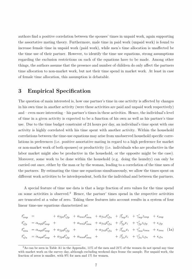
authors find a positive correlation between the spouses’ times in unpaid work, again supportingthe assortative mating theory. Furthermore, male time in paid work (unpaid work) is found toincrease female time in unpaid work (paid work), while men’s time allocation is unaffected bethe time use of their partner. However, to identify the time use equations, strong assumptionsregarding the exclusion restrictions on each of the equations have to be made. Among otherthings, the authors assume that the presence and number of children do only affect the partnerstime allocation to non-market work, but not their time spend in market work. At least in caseof female time allocation, this assumption is debatable.

3 Empirical Specification

The question of main interested is, how one partner’s time in one activity is affected by changesin his own time in another activity (were these activities are paid and unpaid work respectively)and – even more interesting – his partner’s times in these activities. Hence, the individual’s levelof time in a given activity is expected to be a function of his own as well as his partner’s timeuse. Due to the time budget constraint of 24 hours per day, an individual’s time spent with oneactivity is highly correlated with his time spent with another activity. Within the householdcorrelations between the time-use equations may arise from unobserved household specific corre-lations in preferences (i.e. positive assortative mating in regard to a high preference for marketor non-market work of both spouses) or productivity (i.e. individuals who are productive in thelabor market might also be productive in the household, or the opposite might be the case).Moreover, some work to be done within the household (e.g. doing the laundry) can only becarried out once, either by the man or by the woman, leading to a correlation of the time uses ofthe partners. By estimating the time use equations simultaneously, we allow the times spent ondifferent work activities to be interdependent, both for the individual and between the partners.

A special feature of time use data is that a large fraction of zero values for the time spendon some activities is observed.2 Hence, the partner’ times spend in the respective activitiesare truncated at a value of zero. Taking these features into account results in a system of fourlinear time-use equations characterized as:

t∗imp = + αfp1t∗

ifp + αmu1t∗imu + αfu1t∗

ifu + β′mpxi + γ′

mpzimp + εimp

t∗ifp = αmp2t∗

imp + + αmu2t∗imu + αfu2t∗

ifu + β′fpxi + γ′

fpzifp + εifp

t∗imu = αmp3t∗

imp + αfp3t∗ifp + + αfu3t∗

ifu + β′muxi + γ′

muzimu + εimu (1a)

t∗ifu = αmp4t∗

imp + αfp4t∗ifp + αmu4t∗

imu + + β′fuxi + γ′

fuzifu + εifu

2As can be seen in Table A1 in the Appendix, 11% of the men and 21% of the women do not spend any timewith market work on the survey day, although excluding weekend days frome the sample. For unpaid work, thefraction of zeros is smaller, with 9% for men and 1% for women.

7

tijk =

⎧⎪⎨⎪⎩

t∗ijk if t∗

ijk > 0

0 otherwise(i = 1, ..., N ; j = m, f ; k = p, u) (1b)

where t∗ijk is the latent number of minutes spent on activity k (that is paid or unpaid work) by

household member j (that is male or female) in household i (i = 1, ..., N). The actual observedminutes tijk will equal t∗

ijk if t∗ijk is non-negative and zero otherwise. xi and zijk represent vectors

of explanatory variables included in all equations and equation-specific variables respectively.εijk is the error term.

The coefficients of basic interest are αjk1, αjk2, αjk3 and αjk4. They represent how an indi-viduals time spent in activity k is affected by changes in its own time in the opposite activityand its partner’s times in the same and the opposite activity. However, the correspondingvariables t∗

imp, t∗ifp, t∗

imu and t∗ifu on the right hand side of equations (1) are not exogenously

determined, but themselves choice variables. In order to identify causal effects of changes inthe partners’ time use, we need to search for exogenous variations in the partner’s times in paidand unpaid work. The problem of finding such instruments will be discussed in more detail later.

In order to estimate simultaneous-equation models with limited dependent variables andendogenous regressors, different methods have been proposed; see Amemiya (1978, 1979),Heckman (1978), Smith and Blundell (1986) and – for a discussion of the asymptotic rela-tive efficiency of these estimators – Blundell and Smith (1989). Here, a two-stage proceduredeveloped by Nelson and Olson (1978) is applied. The advantage of this method is that it isrelatively simple to implement. Nevertheless, estimates obtained by this method are consistentand asymptotic normal. The procedure is as follows.

In the first step, the reduced form representation from equation (1) is formed, that is:

t∗imp = π′

mpxi + δ′mp1zimp + δ′

fp1zifp + δ′mu1zimu + δ′

fu1zifu + νimp

t∗ifp = π′

fpxi + δ′mp2zimp + δ′


fu2zifu + νifp

t∗imu = π′

muxi + δ′mp3zimp + δ′


fu3zifu + νimu (2a)

t∗ifu = π′

fuxi + δ′mp4zimp + δ′


fu4zifu + νifu

tijk =

⎧⎪⎨⎪⎩

t∗ijk if t∗

ijk > 0

0 otherwise(i = 1, ..., N ; j = m, f ; k = p, u) (2b)

Equations (2) are estimated by applying maximum likelihood estimates to each of the fourequations separately. From the estimates for π′

jk and δ′, fitted values t̂∗imp, t̂∗

ifp, t̂∗imu and t̂∗

ifu

8

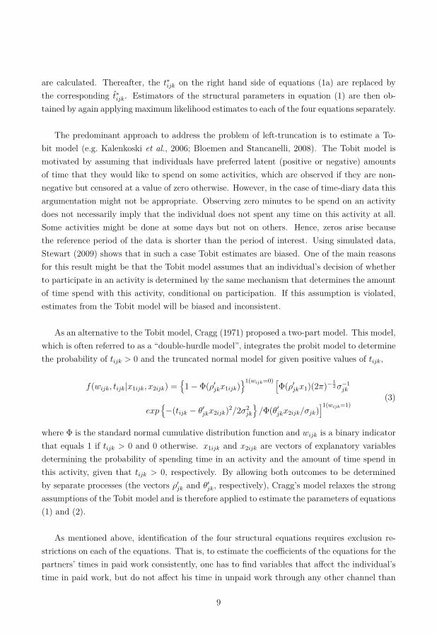
are calculated. Thereafter, the t∗ijk on the right hand side of equations (1a) are replaced by

the corresponding t̂∗ijk. Estimators of the structural parameters in equation (1) are then ob-

tained by again applying maximum likelihood estimates to each of the four equations separately.

The predominant approach to address the problem of left-truncation is to estimate a To-bit model (e.g. Kalenkoski et al., 2006; Bloemen and Stancanelli, 2008). The Tobit model ismotivated by assuming that individuals have preferred latent (positive or negative) amountsof time that they would like to spend on some activities, which are observed if they are non-negative but censored at a value of zero otherwise. However, in the case of time-diary data thisargumentation might not be appropriate. Observing zero minutes to be spend on an activitydoes not necessarily imply that the individual does not spent any time on this activity at all.Some activities might be done at some days but not on others. Hence, zeros arise becausethe reference period of the data is shorter than the period of interest. Using simulated data,Stewart (2009) shows that in such a case Tobit estimates are biased. One of the main reasonsfor this result might be that the Tobit model assumes that an individual’s decision of whetherto participate in an activity is determined by the same mechanism that determines the amountof time spend with this activity, conditional on participation. If this assumption is violated,estimates from the Tobit model will be biased and inconsistent.

As an alternative to the Tobit model, Cragg (1971) proposed a two-part model. This model,which is often referred to as a “double-hurdle model”, integrates the probit model to determinethe probability of tijk > 0 and the truncated normal model for given positive values of tijk,

f(wijk, tijk|x1ijk, x2ijk) ={1 − Φ(ρ′

jkx1ijk)}1(wijk=0) [

Φ(ρ′jkx1)(2π)− 1

2 σ−1jk

exp{−(tijk − θ′

jkx2ijk)2/2σ2jk

}/Φ(θ′

jkx2ijk/σjk)]1(wijk=1)

(3)

where Φ is the standard normal cumulative distribution function and wijk is a binary indicatorthat equals 1 if tijk > 0 and 0 otherwise. x1ijk and x2ijk are vectors of explanatory variablesdetermining the probability of spending time in an activity and the amount of time spend inthis activity, given that tijk > 0, respectively. By allowing both outcomes to be determinedby separate processes (the vectors ρ′

jk and θ′jk, respectively), Cragg’s model relaxes the strong

assumptions of the Tobit model and is therefore applied to estimate the parameters of equations(1) and (2).

As mentioned above, identification of the four structural equations requires exclusion re-strictions on each of the equations. That is, to estimate the coefficients of the equations for thepartners’ times in paid work consistently, one has to find variables that affect the individual’stime in paid work, but do not affect his time in unpaid work through any other channel than

9

through his time in paid work. Similarly, to estimate the equations for the partners’ times inunpaid work consistently, one has to find variables that affect the individual’s time in unpaidwork directly, but his time in paid work only indirectly via the time spent on paid work. Atthis point it is worth noting that a structural form is only estimated for the second part of thedubble-hurdle model, since interest is directed towards the interrelations between the partners’time allocations for those who actually allocate time to these activities. For the selection equa-tions, the unrestricted reduced form (2) is estimated instead.

The assumptions made regarding the exclusion restrictions on the structural equations are asfollows: In order to identify the paid work equations, I assumed that the housing characteristics,i.e. the ownership of the house/flat the couple is living in, the existence of a dishwasher/dryer,the use of external help (domestic help, nanny, handcrafter etc.), whether additional persons areliving within the household, and the distance to the nearest grocery store affect the partners’times in unpaid work, but do not have a direct impact on their times in paid work. Additionally,male time in paid work is assumed to be unaffected by the number and age of the children, whilethis doesn’t hold true for female employment hours.3 Likewise, in order to identify the unpaidwork equations, I assumed that some job characteristics such as the individual’s occupation,the commuting time to and from the workplace as well as the day of the week (Friday or not),do not have a direct impact on the partners’ times in unpaid work. Moreover, the spouses’time dedicated to non-market work was assumed to be uncorrelated with their working timeregulations, i.e. indicators on whether they are doing shift work or have fixed work schedules.

Identification of the structural equations requires at least as much instruments as endogenousregressors included in each of the four equations. Since the vectors zimp, zifp, zimu and zifu

each consist of more than three elements, all of our four equations are over-identified. Thisallows for applying a test for over-identifying restrictions and thus validating the assumptionsmade regarding the exclusion restrictions. As Hoxby and Paserman (1998) show, standardover-identification tests statistics are biased in the presence of clustered data. To address thisproblem, a heteroscedasticity-robust variant of the Hausman test (cf. Wooldridge, 2002) isapplied.

3When comparing the time allocation of employed couples with and without children, it becomes obviousthat compared to childless women, mothers work significantly less hours in the market, while male workinghours are not affected by parenthood.

10

4 Data and Descriptive Statistics

4.1 The German Time Use Surveys 1991/92 and 2001/02

The following analysis is based on the German Time Use Surveys (GTUS) that were conductedby the Federal Statistical Office in 1991/92 and 2001/02. Both surveys were carried out inthe context of representative quota samples of all private households in Germany. The GTUS1991/92 was conducted in 7,200 households that were interviewed between autumn 1991 andsummer 1992. Information was collected on the time use of all household members aged 12years and older, who were asked to describe the routine of the day in 5-minute intervals on twosubsequent days. A total of 32,000 diary days were collected. The GTUS 2001/02 covers about5,400 households who were interviewed between April 2001 and March 2002. All householdmembers aged 10 years and older had to fill in three time diaries – two on working days andone on Saturday or Sunday – in order to describe the routine of the day in 10-minute inter-vals. Altogether, information about 37,700 diary days exists. Despite these methodologicaldifferences between the surveys both data sets are comparable to each other.4 One distinctivefeature that has to be noted here concerns the definition of childcare time. Whereas in the1991/92-sample time spent with children under the age of 16 is defined as childcare time, inthe 2001/02-sample time with children under the age of 18 is included. However, as it couldbe assumed that the time-intensity of children in that age is very small, this difference shouldnot have an impact on the estimation results.

The advantage of the German time use data, as compared to other time use surveys (e.g.the ATUS), is that both partners’ time uses and individual characteristics can be observed.Moreover, the information is very detailed. About 200 different activities can be distinguishedand in addition to main activities, secondary activities as well as persons who are present andmeans of transport have been surveyed. However, in the following analysis main activities havebeen included only.

The following analysis aims to shed light on the connection between the partners’ timesallocated to paid and unpaid work. These time uses are defined as follows: Paid work includestime dedicated to main and secondary employment, work breaks as well as commuting timeto and from the workplace. Furthermore, times for on-the-job training and job seeking are in-cluded. In the literature, unpaid work is usually defined according to the third-person-criterion(Reid, 1934), i.e. it includes all unpaid tasks that could in principle be delegated to a thirdperson. We follow this categorization. Unpaid work consists of housework (preparing meals,cleaning/keeping up house and yard, doing the laundry, gardening, caring for pets, doing main-tenance and repair, shopping, making use of external services, managing the household, travel

4A comparison of the GTUS 1991/91 and the GTUS 2001/02 can be found in Table A2 in the Appendix.

11

time in connection with these activities) and childcare (feeding the child, bathing the child,educating the child, playing/doing sports with the child, talking to the child, reading to thechild, travel time in connection with child-related activities).5 Analyzing the connection be-tween paid and unpaid work of partners consequently means not including time spent sleepingand leisure time in the analysis.

The sample considered in the following analysis consists of married and cohabiting couplesliving within one household that were selected according to the following criteria:

– both spouses are aged between 18 and 64 years, i.e. they are of working age

– both spouses are employed (full-/part-time)

– both spouses had filled in the time diary on the same day

– both spouses had filled in the time diary on a normal day6

– the household does not contain adult persons in need of care

As interest is directed towards the connection between the partners’ times in paid and unpaidwork, weekdays (Monday till Friday) are included only.7 Further excluding individuals withmissing information on at least one of the variables used in the empirical analysis leads to asample of 2,952 couples and 5,301 diary days.

4.2 Variables

In the empirical analysis several household and individual characteristics are controlled for.Since there are no theoretical arguments to suggest that some factors do either solely affectthe probability to engage in paid or unpaid work or solely affect the amount of time allocatedto these activities, the variables included in the first and the second part of the dubble-hurdlemodel are the same. On the household level, dummy variables for the region the couple is livingin (East vs. West Germany), the sample period (1991/92 vs. 2001/02) and an interaction of

5Some authors argue that the utility associated with childcare is different from the utility generated byordinary housework and thus the two have to be analyzed separately (see e.g. Deding and Lausten, 2006;Kimmel and Connelly, 2007). I would have followed this approach, but for lack of instruments solely affectinghousework and childcare respectively, in this analysis both tasks had to be combined.

6As individuals themselves had to decide whether the day is a normal or a non-normal day, an exclusionof non-normal days is debatable. Therefore, the same analysis has been carried out including all diary days.However, the results didn’t change significantly, thus they are not presented here.

7It is worth noting that this might result in underestimating male non-market work, since men tend todo relatively more household and childcare tasks on weekends. However, since time pressure is much higherduring the week compared to the weekend, because many of the non-market tasks cannot be postponed untilthe weekend (e.g. taking the children to school, preparing meals etc. ), but have to be done at fixed times ofthe week, main interest is directed towards the interrelations of the partners’ time uses during the week.

12

both are included. Additionally, the household income, the couples’ marital status (cohabitingor married), the number of children, and the age of the youngest child are controlled for. Onthe individual level, the age of the partners, their schooling and vocational education (4 and 6dummies, respectively), and their net hourly wages are controlled for.

Concerning the income information, some remarks are necessary. First, information onmonthly net earnings was collected both as a continuous variable and in intervals, for respon-dents who did not provide continuous earnings information. For them, earnings are set equalto the mid-point of each interval, and to the lower bound of the top interval. Second, earningsinformation was collected in Deutsche Mark (DM) in 1991/92 (1 euro equals 1,95583 DM) andin euros in 2001/02. Even if converting the 1991/92-earnings into euros, both measures arenot comparable to each other, due to inflation and a considerable growth in wages over thisperiod. In addition, this wage growth was much more pronounced in East compared to WestGermany (Gernandt and Pfeiffer, 2008)). I address this problem by interacting the earningsvariable with the dummy for the sample period.8 Third, the direction of causality between anindividual’s earnings and its time allocation (especially its allocation of time to market work) isnot clear cut. On the one hand, the partners’ relative earnings could serve as a proxy for theirbargaining power within the household and therefore affect the division of paid and unpaid workbetween the spouses. On the other hand, an individual’s working time has a direct impact onits earnings, so that a reverse causation between earnings and working time exists. A commonway to address this problem is replacing actual wages by predicted wages and using the latteras control variables in the regression. As information on standard wage predictors is scarcein the data (primarily, information on the working experience of the individuals is missing),predicting the partner’s wages was not possible. However, as hourly wages, i.e. monthly netearnings divided by usual working hours, instead of monthly wages are included, the problemof reverse causality should be of minor relevance here.

In addition, instruments for the partners’ times spent in paid and unpaid work are includedin the regressions. As instruments for the unpaid work equations, dummy variables indicatingthe ownership of the house/flat the couple is living in, the existence of a dishwasher/dryer, theuse of external help (domestic help, nanny, handcrafter etc.), whether additional persons areliving within the household as well as a variable containing the distance to the nearest grocerystore are included. As mentioned in Section 3, the number and the age of the children serveas additional instruments for male time dedicated to unpaid work, while they could not beapproved to be valid instruments for female time in unpaid work. To identify the paid workequations, dummies for the spouses’ occupation, their working time regulations (indicatingwhether they have fixed work schedules or shift work), the day of the week (Friday or not) and

8As both aspects also apply to the information on household income, the same was done for this variable.

13

a variable containing the individuals’ commuting time to and from the workplace are includedas instruments. Descriptive statistics of these variables are given in Table A3 in the Appendix.

4.3 Couples’s Time Allocation

Figure 1 shows the daily minutes men and women allocate to paid and unpaid work as well asthe total daily workload of the partners. In all cases, individuals spending non-zero minutes inthe respective activity are included only. In 1991/92, West German men spend about 9 hoursand West German women about 6 hours in paid work on an average working day. Ten yearslater, the difference between the sexes becomes smaller, since women increased their workinghours (by about half an hour), while men’s working hours stayed almost constant. In EastGermany, both men and especially women do work longer hours in the market and the divisionof market work between the sexes is much more equal compared to West Germans. From the1990s to 2001, both men and women slightly decreased their working hours (by about 20 min-utes for men and 15 minutes for women), but the ratio between the sexes stays almost constant.The finding of East German women working considerably more hours in the market comparedto West German women is not surprisingly and can be explained by the East Germans’ institu-tional background prior to German reunification. In the former German Democratic Republic,almost all women had been full time employed, thus still today female (full-time) employmentis much more usual in East Germany compared to West Germany.

< Figure 1 about here >

Regarding the partners’ times in unpaid work in West Germany in the 1990s, one can seethat with an average workload of 5.5 hours per day, women do the bulk of the couples’ house-hold work, while men spend less than 2 and a half hours. In 2001/02, the difference betweenthe sexes becomes smaller, but this is mainly due to women having reduced their time in non-market work, while men’s time in non-market work increased only slightly. Compared to WestGermany, the division of unpaid labor between the sexes is more equal in East Germany, withmen spending about 2.5 and women about 4.5 hours in non-market work. From 1991 to 2001,both men and women in East Germany reduced their time in unpaid work. But similar tothe allocation of time to paid work, the female share of time in unpaid work stayed almostconstant. In sum, both East and West German couples decreased their time in unpaid workover one decade, a fact that may partly be explained by technological progress, i.e. the increas-ing utilization of home appliances like dishwashers, microwaves etc. or the rise in demands onexternal home help.

The total working time of the couple is higher in the Eastern part of Germany, where menand women spend about 21 hours with paid or unpaid work per weekday, compared to 19.5

14

hours for West German couples. However, although East and West German couples differ intheir intra-household allocation of time to market and non-market work, the total workloadof the household is shared equally between the partners in both parts of the country. Thisgoes against the widely held belief that – with an increase in female participation in the labormarket – women have to bear a double burden of both being employed and being responsiblefor the household (and – if present – for the children).9

Despite these differences in the time allocation of the four subsamples, the following em-pirical analysis is conducted for the sample as a whole. For a separate analysis, the numberof observations, especially in the East German sample, would have been too small. To allowfor differences in the time allocation of East and West German couples and changes over time,dummy variables for the region, the sample period as well as an interaction between the twohave been included in the regression.

5 Empirical Results

5.1 Reduced form estimates

Table 1 shows the estimation results of the reduced form equations (2) for the partners’ timesspend with paid work. Marginal effects of the probit regression in the first part of the dubble-hurdle model are included in columns 1 and 3 along with their standard errors. For men,hardly any variables show a significant impact on the probability of spending any time withemployment on the survey day. In contrast, womens’ employment probability is highly affectedby the number and age of her children. Moreover, the probability of spending time with mar-ket work decreases by womens’ age, probably reflecting that younger women are more likelyto work full-time compared to older ones. Lastly, womens’ employment probability is affectedby their vocational education and increasing with their wage rate. The results indicate thatthe reason for not spending any time with employment on the survey day differs by gender.Observing a woman to spend zero minutes with market work might most likely be due to thewoman working part-time and being observed on a non-working day. For men, a clear-cutreason for not working on the survey day cannot be found, since almost all men are full-timeemployed (only 3% of the men declared to work part-time, compared to 46% of the women).These results support the importance of applying an econometric specification that allows thedecision of spending time with employment and the minutes of time spend with employmentconditional on participation to be determined by different factors.

9However, it should be kept in mind that main activities are considered only. If women (or men) are morelikely to do working tasks simultaneously, their total workload will be underestimated.

15

< Table 1 about here >

The results of the second part of the dubble-hurdle model for male and female minutes spendwith market work are shown in columns 2 and 4 of Table 1. As expected, the couples’ house-hold income is positively correlated with both partners’ working hours. Moreover, cohabitingwomen spend significantly more minutes in market work compared to those being married. Onthe individual level, both partners’ employment hours are found to decrease by age. Moreover,men’s employment hours vary by their vocational education. While female working hours aresignificantly decreasing with the number and presence of small children, mens’ working hoursare not affected by children. Regarding the effects of the instruments used in the paid workequations, doing shift-work is found to increase female employment hours. Furthermore, femaleblue-collar workers and women being self-employed work less minutes in the markets comparedto white collar workers. In contrast to women, men being self-employed work longer hoursin the market, while the opposite is true for civil servants. Compared to other days of theweek, both men and women spend less minutes with employment on Fridays and their workingtime increases by the distance to the workplace. Joint significance of the instruments can beconfirmed by the corresponding F-tests (values 39.55 and 18.73 for male and female workingtime respectively).

The results of the reduced form equations for male and female time spend with unpaid workare shown in Table 2. Since the proportion of women not spending any time with non-marketwork on the survey day is very low (less than 1%), the first-step probit model could only beestimated for men. For them, the probability of spending time with unpaid work is increasingwith the presence of small children in the household. Moreover, self-employed are less likely toengage in non-market work compared to white collar workers.


Regarding the results of the second-part of the dubble-hurdle model (columns 2 and 4),the truncated regressions for the partners’ minutes spend in unpaid work, cohabiting womenare found to spend significantly less minutes in non-market work compared to those married.Together with the positive effect of cohabitation on female employment hours, this finding iscontrary to Becker’s theory of marriage (Becker, 1973, 1974). According to him, marriage leadsto a specialization of two spouses within a household, in a way that the partner with the higherearnings potential (which will in most instances be the man) specializes in market work, whilethe one with the lower earnings potential specializes in housework. However, since the propor-tion of couples being married is increasing by the age of the partners, this might partly reflect agenerational effect, with older couples having a more traditional division of labor compared to

16

younger ones. This finding is supported by the fact that female non-market hours are increasingby age. Moreover, both spouses’ time spend with unpaid work is highly affected by the numberand age of their children. From the other instruments, living in an owner-occupied dwellingis found to have a significant positive impact on both partners’ time spend with unpaid work.Male time in non-market work is further increasing with the distance to the nearest grocerystore. While having a dishwasher is reducing male time in non-market work, it is increasing fe-male time in non-market work (both effects are significant at a 10-percent level only). Whereastoweling the dishes seems to be a typical male task, (un-)loading the dishwasher seems to bea female task. Moreover, women’s time in unpaid work is significantly higher in householdscontaining additional persons, which might be older people, e.g. the partners’ parents, thatare cared for. Regarding the results of the F-tests for joint significance of the instruments,instrument weakness can be ruled out for the female equation, while the value of 8.9 for themale equation is slightly below the critical threshold of F = 10 for power in IV models.

By and large, the estimation results of the determinants of the partners’ times allocated tomarket and non-market work confirm those expected by theoretical consideration and found inprevious studies.

5.2 Structural form estimates

Full structural form estimates for the partners’ times allocated to paid and unpaid work canbe found in Table A4. Since the reduced instead of the structural form is estimated for theselection equations, second-part results are reported only. The effects of main interest – theinterdependencies between the time uses of the partners – are shown in Table 3.


Regarding male time in paid work, it becomes obvious that none of the coefficients of theendogenous regressors is significant. Male time spent in market work is fixed, i.e. men’s em-ployment hours are neither affected by their own time spent with non-market work, nor bytheir wife’s time allocation (to market and non-market work). In contrast, female time in paidwork is highly affected by her partner’s time allocation: The more time the men dedicates tomarket work, the more time the women dedicates to market work as well. This could be anindicator for assortative mating being relevant in this context, in a way that individuals witha high preference for market work select themselves together. Moreover, it is consistent withthe finding of Hamermesh (2002), who provides evidence that couples attempt to synchronizetheir work schedules in order to increase their joint leisure time. Female time in paid work isfurther increasing by male time allocated to unpaid work. Thus, men who engage in householdand childcare tasks can take some time pressure off from their wife, who on her part is able to

17

increase her employment hours. Since for employees time pressure is considerably higher duringweekdays compared to the weekend, this effect might partly be driven by restricting the analysisto weekdays. Lastly, the wife’s own time allocated to non-market work is significantly reducingher time allocated to market work, which is merely a consequence of the time budget constraint.

The results for the partners’ times spend with unpaid work show that mens’ time allocationis unaffected by the time allocation of their partner. In contrast, female time dedicated to non-market work is found to be negatively affected by her partners’ time in paid and unpaid work.Hence, womens’ non-market workload is highly depending on the support by their partner. Asexpected, for both partners their own time in market work has a significant negative impact ontheir time in non-market work.

As mentioned above, the unbiasedness of the estimation results critically relies on the va-lidity of the exclusion restrictions. The p-values of the respective χ2-tests on over-identifyingrestrictions range from 0.36 for female time in paid work to 0.92 for male time in paid work.Hence, for all equations the null-hypothesis of valid exclusion restrictions can’t be rejected andwe can be confident about the validity of the instruments. For comparison, Table A5 shows theestimation results for the the interdependencies between the time uses of the partners apply-ing a Tobit model instead of the double-hurdle model. The results are similar to those of thedubble-hurdle model, except for male time dedicated to market work, which is now significantlyaffected by female time allocated to market and non-market work. However, as the consistencyof the Tobit estimates critically rests on the assumption that an individual’s decision of whetherto participate in an activity is determined by the same mechanism that determines the amountof time spent with this activity, these results are at risk of being biased.

In sum the results help us getting an idea of the couples’ decision making process regardingthe division of labor between the partners. It seems that in the first instance, the male partnerdetermines his time allocated to market work. Consequently, the more time he spends withmarket work, the less time he spends with non-market work. Male non-market time, on theother hand, determines the amount of time the wife spends with unpaid work. Finally, onthe basis of the amount of time left, the decision about her working hours is made. Theinterdependency between women’s non-market and market hours might be particularly strongfor couples with (small) children, as in most cases childcare tasks (such as feeding/dressingthe children, taking them to the kindergarten and to the school respectively etc.) have tobe done at fixed times of the day. Dividing non-market work into housework and childcareand analyzing both tasks separately may provide some further insights into the couples’ timeallocation decisions. However, due to the lack of instruments solely affecting housework andchildcare respectively, analyzing both tasks separately wasn’t possible here.

18

6 Conclusion

The aim of this paper was to shed light on the intra-household division of labor of Germancouples, more precisely, the interactions between the time allocations of the partners withinone household. It contributes to the existing literature by employing a structural interdepen-dent model of the spouses’ time allocation to market and non-market work, that allows forsimultaneity and endogeneity of the time uses of the partners. For estimation, a dubble-hurdlemodel proposed by Cragg (1971) is applied, that allows the probability of spending time in anactivity and the amount of time spend in this activity, conditional on participation to be de-termined by separate processes and therefore relaxes the strong assumptions of the Tobit model.

The major finding is that men’s time allocation to paid and unpaid work is unaffected bytheir wives’ time allocation, while women adjust their working hours to the time allocation oftheir partner. This finding suggests that within the household, men can avail themselves of a“first mover advantage”, i.e. they decide about their amount of time dedicated to market andnon-market work first. On the basis of male time allocation, which constitutes a fixed parame-ter in the female time allocation decision, women in turn choose their optimal amount of timededicated to market and non-market work. Thereby, the more their husband supports themin the field of non-market work, the more time and effort they are able to invest in market work.

Although the widely spread belief of women’s total workload exceeding that of men’s ifboth partners are employed doesn’t prove true for the case of Germany, German women stillbear a double burden of being responsible for household and children and being active in thelabor market. The amount of time being left for the latter thereby substantially depends onthe domestic support of her partner. This finding might provide a further explanation for stillpersisting gender differences in respect of wages and promotion prospects in Germany. On theone hand, employers may assume women to be less productive in the labor market and thereforebe more likely to hire or promote men instead. On the other hand, women themselves may seeklower payed or less promising jobs that are characterized by a higher flexibility in schedulingand therefore compatible with their responsibility for household and children.

It is obvious that the division of labor of German spouses would become more equal ifmen increased their engagement in non-market work, which would raise their wife’s amountof time disposable for market work. However, as policy makers cannot affect intra-householdtime allocation directly, they should at least aim for providing a working environment thatoffers a maximum of flexibility. This includes regulations regarding working time flexibilities,parental leave regulations as well as the provision of childcare services, which would lower theopportunity costs of market work for women. However, evidence also suggests that within thelast decade, the division of labor between men and women has become much more equal in

19

(West) Germany. If this trend persists, gender differences in labor market prospects and wagesmay be diminishing.

20

References

Amemiya, T. (1978). The Estimation of a Simultaneous Equation Generalized Probit Model.Econometrica, 46 (5), 1193–1205.

— (1979). The Estimation of a Simultaneous-Equation Tobit Model. International EconomicReview, 20 (1), 169–181.

Becker, G. S. (1965). A Theory of the Allocation of Time. The Economic Journal, 75 (299),493–517.

— (1973). A Theory of Marriage: Part I. The Journal of Political Economy, 81 (4), 813–846.

— (1974). A Theory of Marriage: Part II. The Journal of Political Economy, 82 (2), S11–S26.

Bloemen, H. G. and Stancanelli, E. G. F. (2008). How Do Parents Allocate Time? TheEffects of Wages and Income. IZA Discussion Paper No. 3679.

Blundell, R. W. and Smith, R. J. (1989). Estimation in a Class of Simultaneous EquationLimited Dependent Variable Models. The Review of Economic Studies, 56 (1), 37–57.

Chiappori, P.-A. (1988). Rational Household Labor Supply. Econometrica, 56 (1), 63–90.

Connelly, R. and Kimmel, J. (2007). Spousal Influences on Parents’ Non-Market TimeChoices. IZA Discussion Paper No. 2894.

Cragg, J. G. (1971). Some Statistical Models for Limited Dependent Variables with Appli-cation to the Demand for Durable Goods. Econometrica, 39 (5), 829–844.

Deding, M. and Lausten, M. (2006). Choosing between his time and her time? Paid andunpaid work of Danish couples. electronic International Journal of Time Use Research, 3 (1),28–48.

Gernandt, J. and Pfeiffer, F. (2008). Wage Convergence and Inequality after Unification:(East) Germany in Transition. SOEPpapers on Multidisciplinary Panel Data Research 107.

Hamermesh, D. S. (2002). Timing, togetherness and time windfalls. Journal of PopulationEconomics, 15, 601–623.

Heckman, J. J. (1978). Dummy Endogenous Variables in a Simultaneous Equation System.Econometrica, 46 (4), 931–959.

Hersch, J. and Stratton, L. S. (1994). Housework, Wages, and the Division of HouseworkTime for Employed Spouses. The American Economic Review, 84 (2), 120–125.

21

Hoxby, C. and Paserman, M. D. (1998). Overidentification tests with grouped data. Na-tional Bureau of Economic Research, Technical Working Paper 223.

Kalenkoski, C. M., Ribar, D. C. and Stratton, L. S. (2006). The Influence of Wageson Parents’ Allocations of Time to Child Care and Market Work in the United Kingdom.,IZA Discussion Paper No. 2436.

Kimmel, J. and Connelly, R. (2007). Mother’s Time Choices. Caregiving, Leisure, HomeProduction, and Paid Work. The Journal of Human Resources, 42 (3), 643–681.

McElroy, M. B. and Horney, M. J. (1981). Nash-Bargained Household Decisions: Towarda Generalization of the Theory of Demand. International Economic Review, 22 (2), 333–349.

Nelson, F. and Olson, L. (1978). Specification and Estimation of a Simultaneous-equationModel with Limited Dependent Variables. International Economic Review, 19 (3), 695–709.

Reid, M. G. (1934). Economics of household production. New York, London: J. Wiley & SonsInc. and Chapman & Hall Limited.

Smith, R. J. and Blundell, R. W. (1986). An Exogeneity Test for a Simultaneous EquationTobit Model with an Application to Labor Supply. Econometrica, 54 (3), 679–685.

Statistisches Bundesamt (2003). Wo bleibt die Zeit? Die Zeitverwendung der Bevölkerungin Deutschland 2001/02. Statistisches Bundesamt. Wiesbaden, Germany.

Stewart, J. (2009). Tobit or Not Tobit? IZA Discussion Paper No. 4588.

Wooldridge, J. M. (2002). Econometric analysis of cross section and panel data. Cambridge,MA: MIT Press.

22

Figures

Figure 1: Partners’ daily workload

551

355

540

387

590

497

569

482

0

120

240

360

480

600

1991/92 2001/02 1991/92 2001/02

West Germany East Germany

Male Female

Dai

ly m

inut

es

(a) Paid work

139

339

149

281

154

261

151

221

0

60

120

180

240

300

360

1991/92 2001/02 1991/92 2001/02


Male Female

Dai

ly m

inut

es(b) Unpaid work

636597 594 574

683 699

636 615

0

120

240

360

480

600

720

1991/92 2001/02 1991/92 2001/02


Male Female

Dai

ly m

inut

es

(c) Total work

23

Tables

Table 1: Reduced form estimates – Paid workMale Female

P(t>0) E(t|t>0) P(t>0) E(t|t>0)Exogenous regressors:Constant 1.225∗∗∗ 541.133∗∗∗ 1.691∗∗∗ 437.705∗∗∗

(0.29) (24.43) (0.23) (29.87)East Germany 0.031 19.329∗∗ 0.031 81.784∗∗∗

(0.02) (9.84) (0.03) (10.81)Wave 1991/92 0.107∗∗∗ 37.895∗ −0.061 −7.419

(0.04) (19.65) (0.05) (23.03)East Germany*Wave 1991/92 −0.041 −1.582 0.119∗∗∗ 46.362∗∗∗

(0.03) (12.17) (0.04) (14.40)Cohabiting 0.019 0.369 0.045 37.317∗∗∗

(0.02) (11.74) (0.04) (11.77)Household net income (in 1,000¤) 0.004 10.900∗∗ −0.005 15.490∗∗∗

(0.01) (4.98) (0.01) (5.42)Household net income (in 1,000¤)*Wave 1991/92 0.003 15.230∗∗ 0.028∗ 16.556∗∗

(0.01) (6.48) (0.02) (7.43)Age −0.001 −1.098∗∗∗ −0.004∗∗∗ −1.922∗∗∗

(0.00) (0.35) (0.00) (0.47)Net hourly wages (in ¤) 0.000 −0.050 0.001∗∗ 0.101∗

(0.00) (0.06) (0.00) (0.06)Net hourly wages (in ¤)*Wave 1991/92 −0.003∗∗ −5.598∗∗∗ −0.005∗∗ −7.173∗∗∗

(0.00) (1.14) (0.00) (1.50)Schooling (ref.: lower school degree)No degree/other degree 0.000 3.835 −0.021 1.488

(0.01) (6.01) (0.02) (8.40)Degree for professional college 0.007 −14.965 −0.034 12.659

(0.02) (10.80) (0.03) (13.68)High school degree −0.002 −10.069 −0.042∗ −9.020

(0.02) (10.25) (0.02) (10.52)Vocational education (ref.: apprenticeship )No education −0.040 −9.476 −0.010 −10.302

(0.03) (15.77) (0.03) (15.43)Master school −0.040∗∗∗ 17.810∗∗ 0.033 13.389

(0.01) (7.05) (0.04) (18.57)University of applied science degree 0.003 20.702∗ 0.085∗∗ 18.744

(0.02) (10.85) (0.03) (11.96)University degree 0.012 2.672 0.131∗∗∗ 15.068

(0.02) (12.22) (0.03) (13.69)Other educational degree −0.026 24.045∗∗ 0.036 13.945

(0.03) (11.10) (0.03) (9.76)To be continued on next page

24

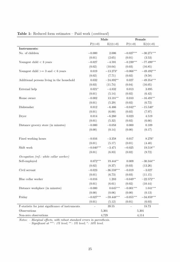
Table 1: Reduced form estimates – Paid work (continued)Male Female

P(t>0) E(t|t>0) P(t>0) E(t|t>0)Instruments:No. of children −0.000 2.006 −0.027∗∗∗ −30.271∗∗∗

(0.01) (2.65) (0.01) (3.53)Youngest child < 3 years −0.027 −4.591 −0.239∗∗∗ −77.499∗∗∗

(0.02) (10.04) (0.03) (16.85)Youngest child >= 3 and < 6 years 0.019 −13.273∗ −0.066∗∗∗ −49.492∗∗∗

(0.02) (7.71) (0.02) (9.58)Additional persons living in the household 0.032 −24.892∗∗ 0.027 −49.354∗∗∗

(0.03) (11.74) (0.04) (16.05)External help 0.021∗ −4.832 0.013 3.895

(0.01) (5.14) (0.02) (6.42)House owner −0.002 13.181∗∗ 0.010 −16.491∗∗

(0.01) (5.29) (0.02) (6.72)Dishwasher 0.012 −6.466 −0.042∗∗ −15.540∗

(0.01) (6.00) (0.02) (7.97)Dryer 0.014 −6.260 0.023 4.519

(0.01) (5.32) (0.02) (6.66)Distance grocery store (in minutes) −0.000 −0.058 0.000 0.109

(0.00) (0.14) (0.00) (0.17)

Fixed working hours −0.016 −3.358 0.017 8.276∗

(0.01) (5.17) (0.01) (4.40)Shift work −0.040∗∗∗ −3.471 −0.025 19.518∗∗

(0.01) (6.83) (0.02) (9.72)Occupation (ref.: white collar worker)Self-employed 0.072∗∗∗ 19.444∗∗ 0.009 −30.344∗∗

(0.02) (8.37) (0.03) (13.26)Civil servant −0.023 −36.559∗∗∗ −0.019 −3.027

(0.01) (6.73) (0.03) (11.15)Blue collar worker −0.016 1.203 −0.049∗∗ −22.572∗∗

(0.01) (6.61) (0.02) (10.44)Distance workplace (in minutes) −0.000 0.645∗∗∗ −0.001∗∗∗ 1.041∗∗∗

(0.00) (0.06) (0.00) (0.13)Friday −0.027∗∗∗ −59.448∗∗∗ −0.055∗∗∗ −34.859∗∗∗

(0.01) (5.12) (0.01) (6.03)F-statistic for joint significance of instruments - 39.55 - 18.73Observations 5,301 5,301Non-zero observations 4,729 4,114Notes: – Marginal effects, with robust standard errors in parenthesis.

– Significant at ∗∗∗: 1% level; ∗∗: 5% level; ∗: 10% level.

25

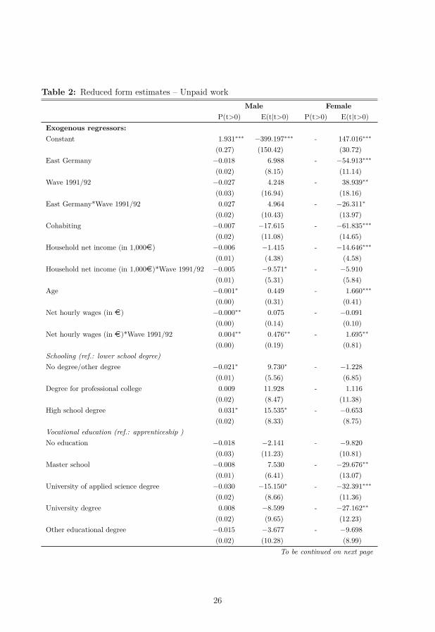
Table 2: Reduced form estimates – Unpaid workMale Female

P(t>0) E(t|t>0) P(t>0) E(t|t>0)Exogenous regressors:Constant 1.931∗∗∗ −399.197∗∗∗ - 147.016∗∗∗

(0.27) (150.42) (30.72)East Germany −0.018 6.988 - −54.913∗∗∗

(0.02) (8.15) (11.14)Wave 1991/92 −0.027 4.248 - 38.939∗∗

(0.03) (16.94) (18.16)East Germany*Wave 1991/92 0.027 4.964 - −26.311∗

(0.02) (10.43) (13.97)Cohabiting −0.007 −17.615 - −61.835∗∗∗

(0.02) (11.08) (14.65)Household net income (in 1,000¤) −0.006 −1.415 - −14.646∗∗∗

(0.01) (4.38) (4.58)Household net income (in 1,000¤)*Wave 1991/92 −0.005 −9.571∗ - −5.910

(0.01) (5.31) (5.84)Age −0.001∗ 0.449 - 1.660∗∗∗

(0.00) (0.31) (0.41)Net hourly wages (in ¤) −0.000∗∗ 0.075 - −0.091

(0.00) (0.14) (0.10)Net hourly wages (in ¤)*Wave 1991/92 0.004∗∗ 0.476∗∗ - 1.695∗∗

(0.00) (0.19) (0.81)Schooling (ref.: lower school degree)No degree/other degree −0.021∗ 9.730∗ - −1.228

(0.01) (5.56) (6.85)Degree for professional college 0.009 11.928 - 1.116

(0.02) (8.47) (11.38)High school degree 0.031∗ 15.535∗ - −0.653

(0.02) (8.33) (8.75)Vocational education (ref.: apprenticeship )No education −0.018 −2.141 - −9.820

(0.03) (11.23) (10.81)Master school −0.008 7.530 - −29.676∗∗

(0.01) (6.41) (13.07)University of applied science degree −0.030 −15.150∗ - −32.391∗∗∗

(0.02) (8.66) (11.36)University degree 0.008 −8.599 - −27.162∗∗

(0.02) (9.65) (12.23)Other educational degree −0.015 −3.677 - −9.698

(0.02) (10.28) (8.99)To be continued on next page

26

Table 2: Reduced form estimates – Unpaid work (continued)Male Female

P(t>0) E(t|t>0) P(t>0) E(t|t>0)Instruments:No. of children −0.004 5.062∗∗ - 38.368∗∗∗

(0.00) (2.25) (2.85)Youngest child < 3 years 0.060∗∗∗ 36.112∗∗∗ - 142.836∗∗∗

(0.02) (7.19) (11.28)Youngest child >= 3 and < 6 years 0.042∗∗∗ 16.204∗∗∗ - 61.961∗∗∗

(0.02) (6.07) (7.73)Additional persons living in the household −0.010 14.172 - 42.869∗∗∗

(0.02) (10.75) (12.56)External help 0.018∗ 0.709 - 0.320

(0.01) (4.62) (5.62)House owner 0.004 7.492∗∗ - 21.189∗∗∗

(0.01) (3.31) (5.74)Dishwasher −0.010 −4.786∗ - 4.152∗

(0.01) (2.62) (2.32)Dryer −0.007 −3.627 - −2.200∗

(0.01) (4.72) (1.31)Distance grocery store (in minutes) −0.000∗∗ 0.230∗∗ - 0.046

(0.00) (0.11) (0.16)

Fixed working hours 0.012 2.370 - −5.541(0.01) (4.66) (5.29)

Shift work 0.020 23.701 - 0.108(0.01) (15.29) (8.18)

Occupation (ref.: white collar worker)Self-employed −0.069∗∗∗ −37.114∗∗∗ - 19.717∗∗

(0.01) (7.86) (9.40)Civil servant 0.020 15.418∗∗∗ - 7.485

(0.01) (5.86) (9.98)Blue collar worker 0.006 3.395 - 10.438

(0.01) (5.64) (8.23)Distance workplace (in minutes) −0.000 −0.231∗∗∗ - −0.242∗∗

(0.00) (0.06) (0.09)Friday 0.004 25.669∗∗∗ - 20.821∗∗∗

(0.01) (3.87) (5.13)F-statistic for joint significance of instruments - 8.92 - 13.13Observations 5,301 5,301Non-zero observations 4,799 5,252Notes: – Marginal effects, with robust standard errors in parenthesis.


27

Table 3: Structural form estimates - Truncated regressionPaid work Unpaid work

male female male femaleMale paid work 0.834∗∗∗ −0.438∗∗∗ −0.284∗∗∗

(0.11) (0.04) (0.10)Female paid work 0.153∗ 0.030 −0.423∗∗∗

(0.09) (0.08) (0.09)Male unpaid work −0.312 1.493∗∗∗ −0.513∗∗∗

(0.26) (0.21) (0.18)Female unpaid work 0.184 −1.371∗∗∗ −0.057

(0.12) (0.22) (0.15)Observations 5,301 5,301 5,301 5,301Non-zero observations 4,729 4,114 4,799 5,252Overidentification-test (p-value) 0.92 0.36 0.66 0.50Notes: – Marginal effects, with robust standard errors in parenthesis.

– Significant at ∗∗∗: 1% level; ∗∗: 5% level; ∗: 10% level.– Full estimation results are shown in table A4 in the Appendix.

28

A Appendix

Table A1: Partners’ time allocation to paid and unpaid workAverage Percentage Average minu-minutes of zeros tes if t>0

Male paid work 496.77 0.11 556.86(219.77) (0.31) (143.78)

Female paid work 314.34 0.22 405.04(227.98) (0.42) (173.86)

Male unpaid work 132.22 0.09 146.05(127.85) (0.29) (126.63)

Female unpaid work 294.14 0.01 296.89(169.78) (0.10) (168.16)

Table A2: German Time Use Surveys1991/92 2001/02

Sampling method quota sample quota sampleCollection period autumn 1991 to

summer 1992spring 2001 to spring2002

No. of households 7,200 5,400Age of household memberssurveyed

12 years and older 10 years and older

No. of household members 16,000 12,600No. of diaries per person 2 3No. of activities 200 230Childcare time included for children

under the age of 16included for childrenunder the age of 18

Intervals 5-minute 10-minuteDetails – main and secon-

dary activities– main and secon-dary activities

– means of transport – means of transport– persons who arepresent

– persons who arepresent

29

Table A3: Descriptive StatisticsHousehold level: mean sdEast Germany 0.27 (0.44)Wave 1991/92 0.64 (0.48)East Germany*Wave 1991/92 0.18 (0.39)Household net income (in 1,000¤) 2.74 (1.09)Household net income (in 1,000¤)*Wave 1991/92 1.53 (1.40)Cohabiting 0.05 (0.21)No. of children 1.35 (1.05)Youngest child < 3 years 0.08 (0.27)Youngest child >= 3 and < 6 years 0.13 (0.33)Additional persons living in the household 0.04 (0.20)House owner 0.62 (0.49)External help 0.38 (0.49)Dishwasher 0.65 (0.48)Dryer 0.42 (0.49)Distance grocery store (in minutes) 12.68 (17.50)

male femaleIndividual level: mean sd mean sdAge 43.47 (8.48) 40.72 (8.25)Net hourly wages (in ¤) 10.26 (16.27) 7.81 (23.17)Net hourly wages (in ¤)*Wave 1991/92 5.80 (6.71) 3.91 (4.37)SchoolingLower school degree/other degree 0.37 (0.48) 0.26 (0.44)Intermediary school degree 0.30 (0.46) 0.45 (0.50)Degree for professional college 0.10 (0.29) 0.06 (0.24)High school degree 0.24 (0.43) 0.22 (0.42)Vocational educationNo education 0.03 (0.17) 0.07 (0.25)Apprenticeship 0.49 (0.50) 0.59 (0.49)Master school 0.16 (0.36) 0.05 (0.21)University of applied science degree 0.12 (0.33) 0.08 (0.27)University degree 0.16 (0.37) 0.11 (0.32)Other educational degree 0.05 (0.21) 0.10 (0.30)OccupationSelf-employed 0.17 (0.38) 0.10 (0.30)Civil servant 0.18 (0.38) 0.09 (0.28)Blue collar worker 0.32 (0.47) 0.12 (0.33)White collar worker 0.32 (0.47) 0.69 (0.46)

Fixed working hours 0.40 (0.49) 0.47 (0.50)Shift work 0.17 (0.38) 0.11 (0.32)Distance workplace (in minutes) 42.23 (38.40) 37.34 (33.82)Friday 13.72 (0.34) 13.72 (0.34)Observations 2,952

30

Table A4: Structural form estimates – Truncated regression (continuation of Table 3)Paid work Unpaid work

male female male femaleExogenous regressors:Constant 132.697∗∗∗ 146.814∗∗∗ 259.287∗∗∗ 163.128∗∗∗

(3.13) (2.69) (29.70) (3.00)East Germany 18.508∗ −16.653 18.475∗∗ −10.393

(10.85) (16.00) (9.36) (12.67)Wave 1991/92 40.186∗∗ −0.458 45.454∗∗ 46.390∗∗

(19.47) (24.78) (18.47) (19.82)East Germany*Wave 1991/92 −6.063 −2.591 −7.114 8.764

(13.56) (16.08) (12.08) (16.19)Cohabiting −4.732 −3.297 −17.684 −44.139∗∗∗

(12.29) (15.39) (12.12) (15.53)Household net income (in 1,000¤) 11.843∗∗ −11.254∗ 2.718 −8.200∗

(4.89) (6.28) (4.59) (4.67)Household net income (in 1,000¤)*Wave 1991/92 9.458 15.191∗∗ −8.035 −0.245

(6.47) (7.28) (5.45) (6.29)Age −0.695∗∗ 1.293∗∗ −0.279 0.019

(0.32) (0.62) (0.34) (0.50)Net hourly wages (in ¤) −0.082 0.007 0.086 −0.007

(0.06) (0.07) (0.14) (0.10)Net hourly wages (in ¤)*Wave 1991/92 −5.051∗∗∗ −4.876∗∗∗ −0.940∗∗ −0.858

(1.11) (1.45) (0.44) (0.96)Schooling (ref.: lower school degree)No degree/other degree 3.885 0.032 12.205∗∗ −3.987

(5.95) (8.25) (5.42) (6.85)Degree for professional college −12.588 15.967 5.866 −0.003

(11.26) (13.64) (8.54) (11.31)High school degree −5.859 −14.626 9.756 −9.690

(11.12) (10.39) (8.35) (8.90)Vocational education (ref.: apprenticeship )No education −14.740 −26.719∗ −17.629 −14.198

(15.79) (15.29) (11.41) (10.83)Master school 20.176∗∗∗ −29.688 −0.300 −19.459

(7.20) (21.61) (6.43) (13.20)University of applied science degree 16.432 −18.560 −9.790 −12.892

(11.79) (13.27) (8.44) (11.65)University degree 0.796 −20.740 −9.833 −0.773

(12.26) (14.91) (9.57) (12.68)Other educational degree 21.488∗ 0.759 −2.799 1.135

(11.30) (9.62) (10.28) (9.11)To be continued on next page

31

Table A4: Structural form estimates – Truncated regression (continued)Paid work Unpaid work

male female male femaleInstruments:No. of children - 0.989 57.191∗∗ 39.169∗∗∗

(8.58) (25.86) (6.44)Youngest child < 3 years - 63.430∗ 228.061∗∗ 136.117∗∗∗

(36.90) (95.40) (26.52)Youngest child >= 3 and < 6 years - 3.667 120.152∗∗ 72.576∗∗∗

(17.95) (52.00) (14.93)Additional persons living in the household - - 112.139 58.480∗∗∗

(74.44) (21.01)External help - - 25.442 8.174

(26.33) (8.45)House owner - - 81.891∗∗ 33.687∗∗∗

(35.07) (8.94)Dishwasher - - −25.715 −3.963

(29.02) (10.10)Dryer - - −1.365 8.691

(28.27) (8.29)Distance grocery store (in minutes) - - 1.148∗ 0.305

(0.50) (0.24)

Fixed working hours −2.117 −0.367 - -(5.30) (6.07)

Shift work 4.638 13.387 - -(9.83) (9.55)

Occupation (ref.: white collar worker)Self-employed 7.712 2.078 - -

(13.16) (14.28)Civil servant −30.502∗∗∗ 10.510 - -

(8.04) (11.38)Blue collar worker 4.923 −9.464 - -

(6.83) (10.41)Distance workplace (in minutes) 0.564∗∗∗ 0.699∗∗∗ - -

(0.08) (0.14)Friday −47.593∗∗∗ 9.283 - -

(8.65) (8.94)Observations 5,301 5,301 5,301 5,301Non-zero observations 4,729 4,114 4,799 5,252Notes: – Marginal effects, with robust standard errors in parenthesis.


32

Table A5: Structural form estimates - Tobit regressionPaid work Unpaid work

male female male femaleMale paid work 0.582∗∗ −0.560∗∗∗ −0.249∗∗

(0.25) (0.05) (0.10)Female paid work 0.515∗∗∗ 0.022 −0.355∗∗∗

(0.14) (0.10) (0.08)Male unpaid work −0.115 0.792∗∗ −0.540∗∗∗

(0.48) (0.34) (0.17)Female unpaid work 0.553∗∗∗ −0.914∗∗ −0.235

(0.21) (0.37) (0.24)Observations 5,301 5,301 5,301 5,301Non-zero observations 4,729 4,114 4,799 5,252Notes: – Robust standard errors in parenthesis.

– Significant at ∗∗∗: 1% level; ∗∗: 5% level; ∗: 10% level.– Control variables are same as in Table A4. Full estimation results areavailable from the author upon request.

33

julia bredtmann the intra-household division of labor – an ... · ruhr economic papers #200 julia...

Documents