Joel Anderson

ST 371-002

Lecture Summary for 2/15/2011

Homework 0

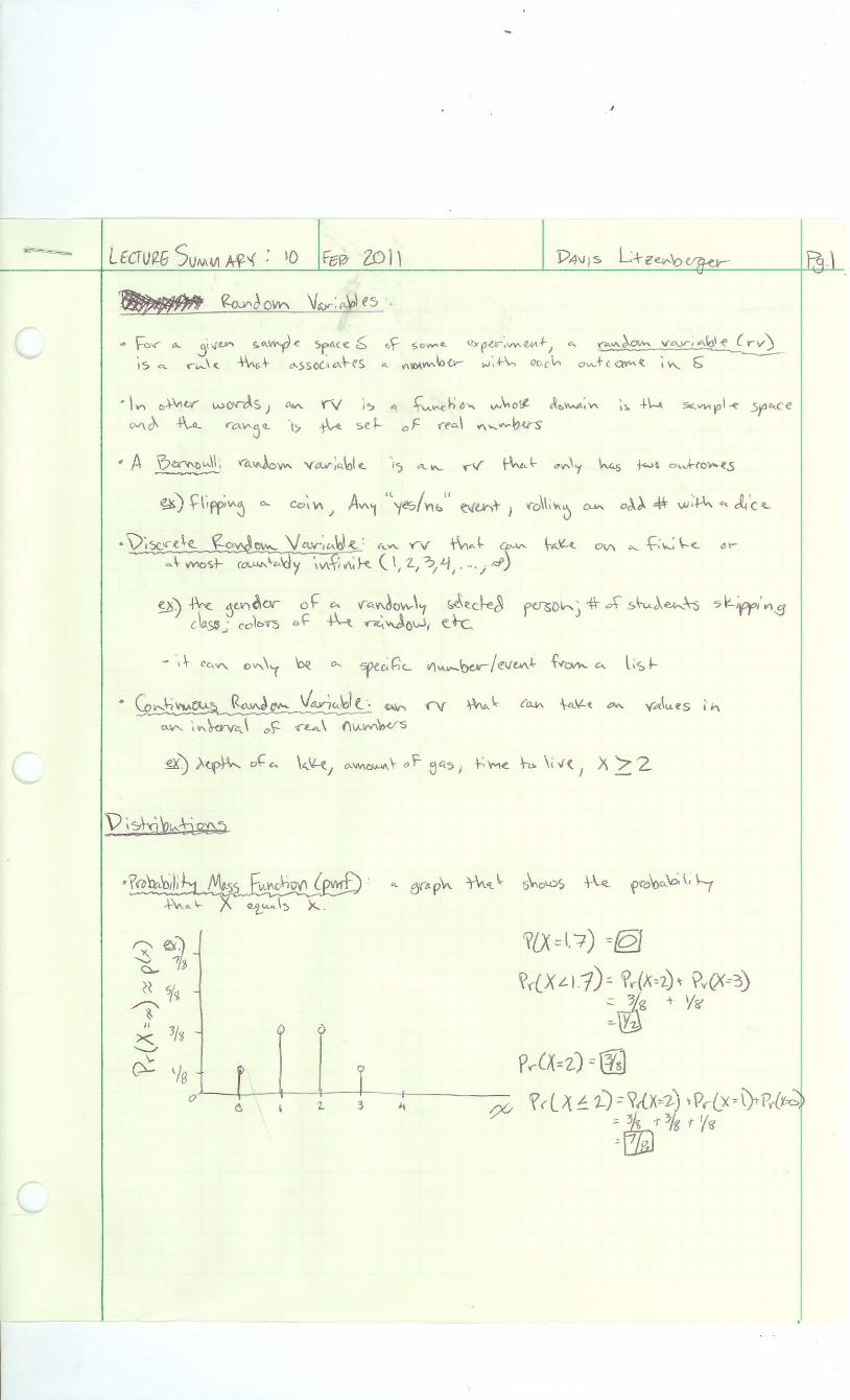
First, the definition of a probability mass function p(x) and a cumulative distribution function

F(x) is reviewed:

Graphically, the drawings of a pmf and a cdf (regarding discrete random variables) are similar to

histograms and step functions. The pmf consists of several lines drawn at each point with the

height scaled to match the relative probability of that event (similar to a histogram). A cdf will

start at zero and increase each time it hits an event on the x axis by a set amount, and then remain

constant until it hits another event, creating a step-like feel. For examples of the two functions,

see Figure 3.3 on page 93 and Figure 3.6 on page 97 of the Devore textbook.

We now turn to finding different characteristics of probability sets that are characterized by

pmf’s and/or cdf’s. First, to find the median of such a set use the cdf to find where F(xp) = ½,

where xp is the median. If an exact value cannot be found, then it must be estimated through

interpolation. An example is shown below:

To find the median, find the 40th

quartile and the 70th

quartile (which are easily found at y=1 and

y=2, respectively). Then we interpolate:

If a probability mass function is not known, it can be derived from the cdf by measuring the

jumps between the ‘steps’ of the cdf. For example, the above function would yield the following

pmf, written as a table for continuous use:

y 0 1 2 3 4 5 6

p(y) 0 0.4 0.3 0.2 0.1 0 0

We can also check our resulting pmf by making sure that all of the values add to 1:

Using this method, we can go back to a pmf from a cdf, or rederive a cdf using integration. In

short, having one of the two makes it possible to get the other.

Next, we look at the expected value of a given pmf, which is symbolized by E(X) or µx

(remember that greek letters correspond to the actual population, while capital letters correspond

to measurements regarding the sample). The expected value of a probability function can be

thought of as the center of mass or balancing point of the function: what is the point that all of

the probabilities are closest to (the average, in essence). We calculate it with the following

formula:

As an example, we can calculate the expected value of the pmf used earlier:

2

y 1 2 3 4

p(y) 0.4 0.3 0.2 0.1

y*p(y) 0.4 0.6 0.6 0.4

For more examples of this calculation or pictures showing the balancing point analogy, see the

section in the Devore textbook starting at page 103.

The variance of a probability function carries the same meaning as it does for other data sets,

however it can be calculated using a shortcut formula that uses the expected value of the

function. This makes calculations of the variance much easier.

We can derive the shortcut formula as shown below:

To demonstrate that using these two formulas gives the same result, we calculate the variance of

the previous function:

y 1 2 3 4

p(y) 0.4 0.3 0.2 0.1

y2*p(y) 0.4 1.2 1.8 1.6

Variance using shortcut method: 0.4 + 1.2 + 1.8 + 1.6 – 22= 5 – 4 = 1

y 1 2 3 4

y-µ -1 0 1 2

(y-µ)2 1 0 1 4

(y-µ)2p(x) 0.4 0 0.2 0.4

Variance using original method: 0.4 + 0 + 0.2 + 0.4 = 1

We see that the two methods yield the same result, but that the shortcut significantly decreases

the amount of work involved (and in turn decreases the opportunity for error in calculation).

Next, we look at what happens to the values when the function is changed in a linear fashion (i.e.

X becomes aX+b). For example, suppose that the function y represented an amount of skittles

each child has in his or her possession. Next, all children are given one skittle, or perhaps each

one is given as many skittles as they have again (doubling their skittles). Is there an easy way to

find the expected value and variance of the new data set without calculating them afresh?

Of course there is, or I wouldn’t be discussing this.

3

This seems too simple to be true. Why would teachers allow crib sheets on tests if formulas were

ever this easy to remember? We can prove that this transformation is correct using the following

derivation:

Unfortunately, the transformations for the variance and standard deviation are not quite as

simple. They are shown below.

Note that b has no effect on the end result. This is because each of the values will still vary from

the expected value (which has shifted by b units, remember) from the same amount that they did

before, meaning that they will not appear in the variance or standard deviation.

To illustrate the concepts of the cdf further, number 23 on page 99 of the Devore text was done

in class. The problem as well as the solutions may be found in the attached handout passed out at

the end of class.

The final topic covered in this lecture is the Bernoulli variable, as well as the binomial variable

formula that typically accompanies this class of variables. A Bernoulli variable is one that may

only take one of two values: success or failure, 0 or 1, pass or fail, etc... The Bernoulli variable

may be used in a the binomial formula when given the probability of success (however success

may be defined is left to the user) is given as p. Bernoulli variables have special properties

regarding variance and the expected value:

And, in general:

With n being the number of trials the variable is given, we may calculate the probability of

having x successes using this formula:

This formula comes from the fact that you can model n trials as a tree with n levels and 2n

terminal nodes. To find the probability of having x number of successes, we label each edge with

the respective probability, find the probability of each path and add them together. That is what

this formula does. For more example problems, see numbers 27, 37, 39, 46, 47, and 71 in

Chapter 3 of the Devore text.

4

5

2/10/11 Lecture Summary

Random Variable function is defined on the sample space of the experiment and assigns a

numerical variable to each possible outcome of the experiment.

It is denoted by capital letters (ex. X, Y, Z)

Probability Distribution or probability mass function (pmf) of a discrete rv is defined for every

number x by p(x)=P(X=x)=P(all s ɛ S: X(s) = x).

Probability of x occurring n # of times

Example: flipping a fair coin three times

The Cumulative Distribution function (cdf) F(x) of a discrete rv variable X with pmf p(x) is

defined for every number x by F(x) = P(X≤x) = ∑p(y). It is the cumulative (add) probabilities of

the experiment for a discrete rv variable.

For any number x, F(x) is the probability that the observed value of X will be at most x.

P(a≤X≤b) = F(b)-F(a-), a- is the largest possible X value that is strictly less than a.

T

1

H

1 T

1 H

1

T

1

H

1

T

1

H

1

H

1

T

1

T

1

H

1

T

1

H

1

X= # of Heads P(x=2) = 3/8 P(x<2) = 1/2 P(x≤2) = 7/8 PMF below

0 1 2 3

3/8

1/8

1 7/8 3/8

1/8

CDF

2/10/11 Lecture Summary

Exercise Section 3.2 #13 in Devore

A mail-order computer business has six telephone lines. Let X denote the number of lines in use

at a specified time. Suppose the pmf of X is as given in the accompanying table.

x 0 1 2 3 4 5 6

P(x) .10 .15 .20 .25 .20 .06 .04

F(x) .10 .25 .45 .70 .90 .96 1

Calculate the probability of each of the following events

a) At most three lines are in use

P(x≤3) = .70

b) Fewer than three lines are in use

P(x<3) = F(2) = .45

c) At least three lines are in use

P(x≥3) = 1-F(2) = 1- .45 = .55

d) Between two and five lines, inclusive, are in use

P(2≤x≤5) = F(5)-F(1) = .96-.25 = .71

e) Between two and four lines, inclusive, are not in use

P(2≤x≤4)’ = F(4)-F(1) = .90-.25 = .65

f) At least four lines are not in use

P(x≥4)’ = F(2) = .45

Lecture Summary Feb 10 Jeffrey Brown

ST371-002

February 10th’s lecture focused on the introduction and discussion of the differences

between discrete and continuous variables. The difference was portrayed showing a tree of

different events with each variable type.

Discrete Continuous

The discrete example shows the discrete random variable X, the number of heads in 3

coin flips. If we recorded every possible outcome after the third flip, we would find all values X

can equal; hence discrete. In the continuous example, the continuous random variable X is the

number of tails recorded in a row. We cannot record all possible values of X in this case since we

can see in the tree there can be anywhere from 0 tails to Ti, or infinite; hence continuous. During

lecture, we discussed how new variables can be introduced to the discrete random variable, such

as Y, the number of heads minus the number of tails, and Z, 2*Y.

The second portion of class we discussed probability mass functions and cumulative

distribution functions. A probability mass function of a discrete random valuable redefines every

number x that the variable X can equal. The graph of the function is then the probability that

X=x. This can be represented by a dot plot with values probability values for each value of x. In

the coin flip example above, the probability that X = 1 is 3/8, since 3 out of the 8 total outcomes

have 3 total number of heads. A cumulative distribution function for a discrete random variable

is similar but instead displays the probability that X is less than or equal to x. This can be

represented by a bar graph with heights between each 2 values of x equal to the probability that

X is within those values. In the coin flip example above, the probability that X is less than or

equal to 2 is 7/8 since 7 out of the 8 possible outcomes has either 2, 1 or 0 total number of heads.

Lecture 6 Summary Will Lowder

Random Variables

Text 3.1,3.2

Cartoon Guide Ch.4

IV in Sun notes

Associating the outcomes from choosing a random variable from a given sample space to certain outcomes

Ex: x=number of heads y=number of tails

x Y 3 3 2 1 1 -1 2 1

A Random Variable (rv) is a function defined on a sample space of an experiment that assigns a value to every possible outcome

Ex: Flipping a coin creates rv X. X({H})=1 and X({T})=0

The Probability Mass Function of an rv is defined by p(x) for every random number x

A Bernoulli random variable is one that only has two possible outcomes

Because the sample space for a coin toss is S={H,T} it is a Bernoulli rv

Define Y=height above sealevel in the US in feet

S={-282=<Y=<14494}

Probability Mass Function is Pr(X=x)

Cumulative Distribution Function is Pr(X=<x)=F(x)

Pr(X=xi)=F(xi)-F(xi-1)

A company has 6 phone lines. The following table represents the probability that a number is in use at a given time

X 0 1 2 3 4 5 6 7 8 P(X) .1 .15 .2 .25 .2 .06 .04 0 0 F(X) .1 .25 .45 .70 .9 .96 1.0 1.0 1.0

Ex. Pr(X=<3)=.70

Pr(x<3)=.45

Pr(X=>3)=1-Pr(X<3)

Pr(2=<X=<5)=F(5)-F(1)