jumpstart mplus

2/18/2010

1

JUMPSTART Mplus

Exploratory and Confirmatory

Factor Analysis

Factor Analysis

Exploratory Factor Analysis (EFA)

A method of data reduction which infers presence of latent

factors which are responsible for the shared variance in a set of

observed variables / items. EFA is by definition ‘exploratory’ - the

user does not specify a structure, and assumes each item/ variable

could be related to each latent factor.

Confirmatory Factor Analysis (CFA)User defines which observed variables /items are related to the specified

constructs or latent factors – based on a priori theory or the results of

EFA

2/18/2010

2

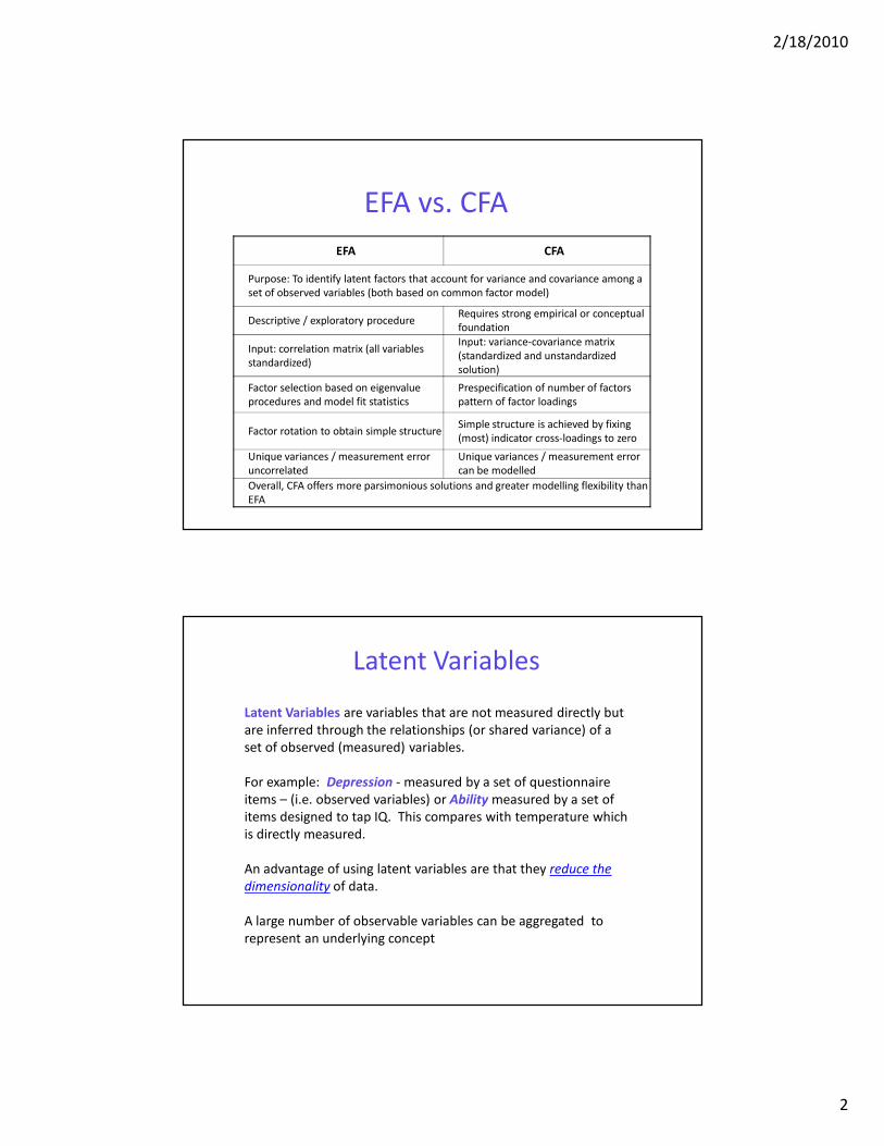
EFA vs. CFA

EFA CFA

Purpose: To identify latent factors that account for variance and covariance among a

set of observed variables (both based on common factor model)

Descriptive / exploratory procedureRequires strong empirical or conceptual

foundation

Input: correlation matrix (all variables

standardized)

Input: variance-covariance matrix

(standardized and unstandardized

solution)

Factor selection based on eigenvalue

procedures and model fit statistics

Prespecification of number of factors

pattern of factor loadings

Factor rotation to obtain simple structureSimple structure is achieved by fixing

(most) indicator cross-loadings to zero

Unique variances / measurement error

uncorrelated

Unique variances / measurement error

can be modelled

Overall, CFA offers more parsimonious solutions and greater modelling flexibility than

EFA

Latent Variables are variables that are not measured directly but

are inferred through the relationships (or shared variance) of a

set of observed (measured) variables.

For example: Depression - measured by a set of questionnaire

items – (i.e. observed variables) or Ability measured by a set of

items designed to tap IQ. This compares with temperature which

is directly measured.

An advantage of using latent variables are that they reduce the

dimensionality of data.

A large number of observable variables can be aggregated to

represent an underlying concept

Latent Variables

2/18/2010

3

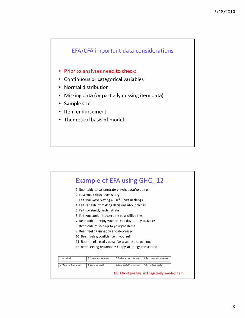
EFA/CFA important data considerations

• Prior to analyses need to check:

• Continuous or categorical variables

• Normal distribution

• Missing data (or partially missing item data)

• Sample size

• Item endorsement

• Theoretical basis of model

Example of EFA using GHQ_12 1. Been able to concentrate on what you’re doing

2. Lost much sleep over worry

3. Felt you were playing a useful part in things

4. Felt capable of making decisions about things

5. Felt constantly under strain

6. Felt you couldn’t overcome your difficulties

7. Been able to enjoy your normal day-to-day activities

8. Been able to face up to your problems

9. Been feeling unhappy and depressed

10. Been losing confidence in yourself

11. Been thinking of yourself as a worthless person.

12. Been feeling reasonably happy, all things considered

1. Not at all 2. No more than usual 3. Rather more than usual 4. Much more than usual

1. More so than usual 2. Same as usual 3. Less useful than usual 4. Much less useful

NB: Mix of positive and negatively worded items

2/18/2010

4

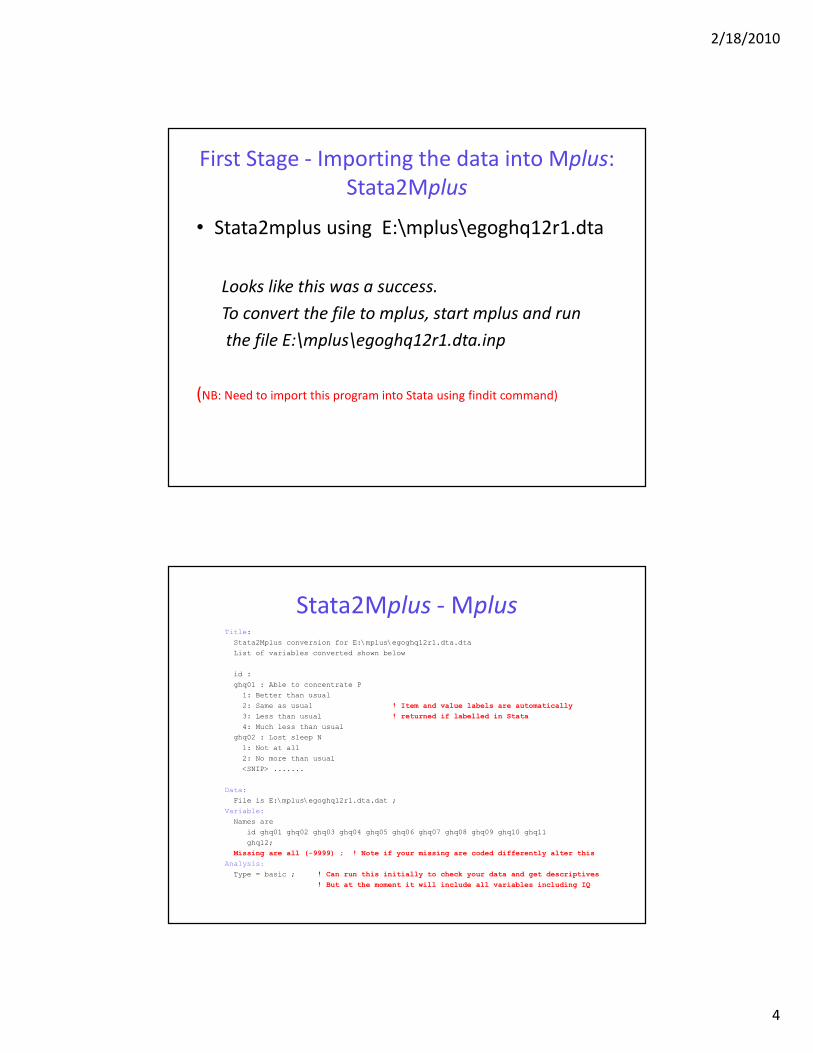
First Stage - Importing the data into Mplus:

Stata2Mplus

• Stata2mplus using E:\mplus\egoghq12r1.dta

Looks like this was a success.

To convert the file to mplus, start mplus and run

the file E:\mplus\egoghq12r1.dta.inp

(NB: Need to import this program into Stata using findit command)

Stata2Mplus - MplusTitle:

Stata2Mplus conversion for E:\mplus\egoghq12r1.dta.dta

List of variables converted shown below

id :

ghq01 : Able to concentrate P

1: Better than usual

2: Same as usual ! Item and value labels are automatically

3: Less than usual ! returned if labelled in Stata

4: Much less than usual

ghq02 : Lost sleep N

1: Not at all

2: No more than usual

<SNIP> .......

Data:

File is E:\mplus\egoghq12r1.dta.dat ;

Variable:

Names are

id ghq01 ghq02 ghq03 ghq04 ghq05 ghq06 ghq07 ghq08 ghq09 ghq10 ghq11

ghq12;

Missing are all (-9999) ; ! Note if your missing are coded differently alter this

Analysis:

Type = basic ; ! Can run this initially to check your data and get descriptives

! But at the moment it will include all variables including IQ

2/18/2010

5

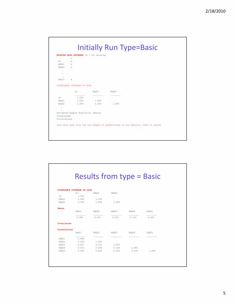
Initially Run Type=BasicMISSING DATA PATTERNS (x = not missing)

1

ID x

GHQ01 x

GHQ02 x

.

.

.

GHQ12 x

COVARIANCE COVERAGE OF DATA

ID GHQ01 GHQ02

________ ________ ________

ID 1.000

GHQ01 1.000 1.000

GHQ02 1.000 1.000 1.000

.

.

Estimated Sample Statistics (means)

Covariances

Correlations

THIS WILL ALSO GIVE YOU THE NUMBER OF OBSERVATIONS IN THE ANALYSIS (IMPT TO CHECK)

Results from type = Basic

COVARIANCE COVERAGE OF DATA

ID GHQ01 GHQ02

ID 1.000

GHQ01 1.000 1.000

GHQ02 1.000 1.000 1.000

Means

GHQ01 GHQ02 GHQ03 GHQ04 GHQ05

________ ________ ________ ________ ________

2.383 2.161 2.132 2.123 2.424

Covariances

Correlations

GHQ01 GHQ02 GHQ03 GHQ04 GHQ05

________ ________ ________ ________ ________

GHQ01 1.000

GHQ02 0.429 1.000

GHQ03 0.407 0.231 1.000

GHQ04 0.475 0.284 0.528 1.000

GHQ05 0.492 0.526 0.252 0.336 1.000

2/18/2010

6

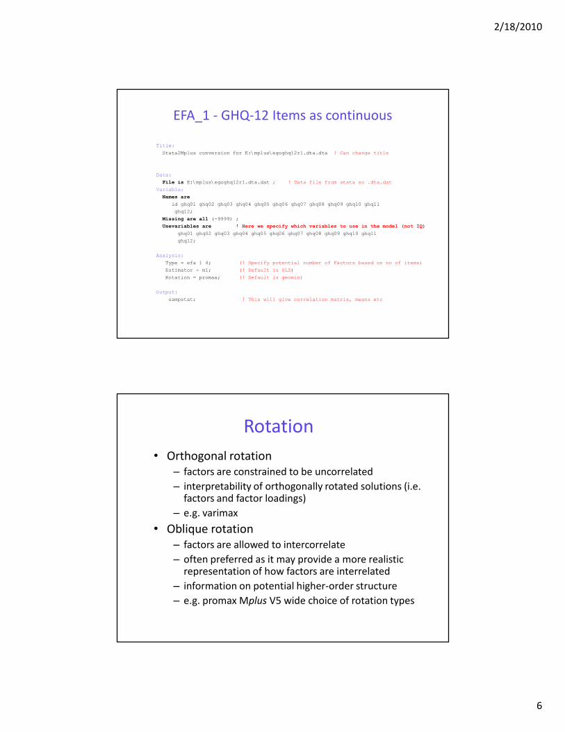
EFA_1 - GHQ-12 Items as continuous

Title:

Stata2Mplus conversion for E:\mplus\egoghq12r1.dta.dta ! Can change title

Data:

File is E:\mplus\egoghq12r1.dta.dat ; ! Data file from stata so .dta.dat

Variable:

Names are


ghq12;

Missing are all (-9999) ;

Usevariables are ! Here we specify which variables to use in the model (not IQ)

ghq01 ghq02 ghq03 ghq04 ghq05 ghq06 ghq07 ghq08 ghq09 ghq10 ghq11

ghq12;

Analysis:

Type = efa 1 4; (! Specify potential number of Factors based on no of items)

Estimator = ml; (! Default is ULS)

Rotation = promax; (! Default is geomin)

Output:

sampstat; ! This will give correlation matrix, means etc

Rotation

• Orthogonal rotation

– factors are constrained to be uncorrelated

– interpretability of orthogonally rotated solutions (i.e. factors and factor loadings)

– e.g. varimax

• Oblique rotation

– factors are allowed to intercorrelate

– often preferred as it may provide a more realistic representation of how factors are interrelated

– information on potential higher-order structure

– e.g. promax Mplus V5 wide choice of rotation types

2/18/2010

7

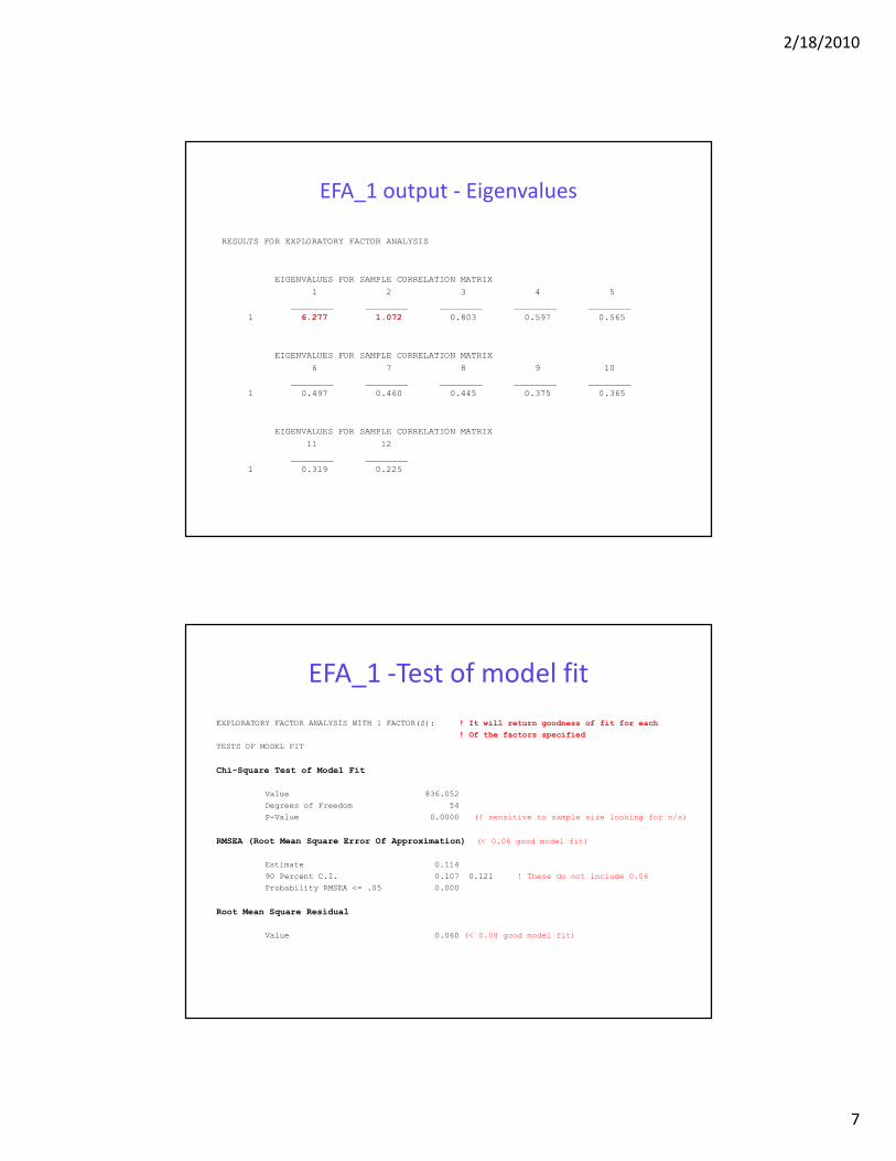
EFA_1 output - Eigenvalues

RESULTS FOR EXPLORATORY FACTOR ANALYSIS

EIGENVALUES FOR SAMPLE CORRELATION MATRIX

1 2 3 4 5

________ ________ ________ ________ ________

1 6.277 1.072 0.803 0.597 0.565


6 7 8 9 10

________ ________ ________ ________ ________

1 0.497 0.460 0.445 0.375 0.365


11 12

________ ________

1 0.319 0.225

EFA_1 -Test of model fit

EXPLORATORY FACTOR ANALYSIS WITH 1 FACTOR(S): ! It will return goodness of fit for each

! Of the factors specified

TESTS OF MODEL FIT

Chi-Square Test of Model Fit

Value 836.052

Degrees of Freedom 54

P-Value 0.0000 (! sensitive to sample size looking for n/s)

RMSEA (Root Mean Square Error Of Approximation) (< 0.06 good model fit)

Estimate 0.114

90 Percent C.I. 0.107 0.121 ! These do not include 0.06

Probability RMSEA <= .05 0.000

Root Mean Square Residual

Value 0.060 (< 0.08 good model fit)

2/18/2010

8

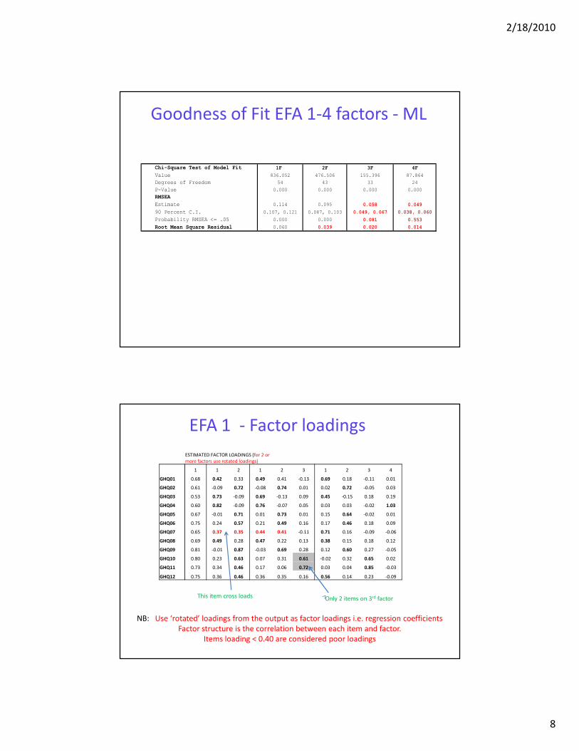
Goodness of Fit EFA 1-4 factors - ML

Chi-Square Test of Model Fit 1F 2F 3F 4F

Value 836.052 476.506 155.396 87.864

Degrees of Freedom 54 43 33 24

P-Value 0.000 0.000 0.000 0.000

RMSEA

Estimate 0.114 0.095 0.058 0.049

90 Percent C.I. 0.107, 0.121 0.087, 0.103 0.049, 0.067 0.038, 0.060

Probability RMSEA <= .05 0.000 0.000 0.081 0.553

Root Mean Square Residual 0.060 0.039 0.020 0.014

EFA 1 - Factor loadings

ESTIMATED FACTOR LOADINGS (for 2 or

more factors use rotated loadings)

1 1 2 1 2 3 1 2 3 4

GHQ01 0.68 0.42 0.33 0.49 0.41 -0.13 0.69 0.18 -0.11 0.01

GHQ02 0.61 -0.09 0.72 -0.08 0.74 0.01 0.02 0.72 -0.05 0.03

GHQ03 0.53 0.73 -0.09 0.69 -0.13 0.09 0.45 -0.15 0.18 0.19

GHQ04 0.60 0.82 -0.09 0.76 -0.07 0.05 0.03 0.03 -0.02 1.03

GHQ05 0.67 -0.01 0.71 0.01 0.73 0.01 0.15 0.64 -0.02 0.01

GHQ06 0.75 0.24 0.57 0.21 0.49 0.16 0.17 0.46 0.18 0.09

GHQ07 0.65 0.37 0.35 0.44 0.41 -0.11 0.71 0.16 -0.09 -0.06

GHQ08 0.69 0.49 0.28 0.47 0.22 0.13 0.38 0.15 0.18 0.12

GHQ09 0.81 -0.01 0.87 -0.03 0.69 0.28 0.12 0.60 0.27 -0.05

GHQ10 0.80 0.23 0.63 0.07 0.31 0.61 -0.02 0.32 0.65 0.02

GHQ11 0.73 0.34 0.46 0.17 0.06 0.72 0.03 0.04 0.85 -0.03

GHQ12 0.75 0.36 0.46 0.36 0.35 0.16 0.56 0.14 0.23 -0.09

NB: Use ‘rotated’ loadings from the output as factor loadings i.e. regression coefficients

Factor structure is the correlation between each item and factor.

Items loading < 0.40 are considered poor loadings

Only 2 items on 3rd factorThis item cross loads

2/18/2010

9

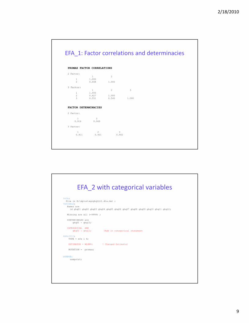
EFA_1: Factor correlations and determinacies

PROMAX FACTOR CORRELATIONS

2 Factor:

1 2

1 1.000

2 0.668 1.000

3 Factor: 1 2 3

1 1.000

2 0.627 1.000

3 0.551 0.540 1.000

FACTOR DETERMINACIES

2 Factor:

1 2

0.916 0.949

3 Factor:

1 2 3

0.911 0.931 0.902

EFA_2 with categorical variables

DATA:

File is E:\mplus\egoghq12r1.dta.dat ;

VARIABLE:

Names are

id ghq01 ghq02 ghq03 ghq04 ghq05 ghq06 ghq07 ghq08 ghq09 ghq10 ghq11 ghq12;


USEVARIABLES are

ghq01 - ghq12;

CATEGORICAL ARE

ghq01 - ghq12; !Add in categorical statement

ANALYSIS:

TYPE = efa 1 4;

ESTIMATOR = WLSMV; ! Changed Estimator

ROTATION = promax;

OUTPUT:

sampstat;

2/18/2010

10

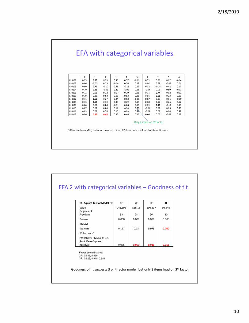
EFA with categorical variables

Difference from ML (continuous model) – item 07 does not crossload but item 12 does

1 1 2 1 2 3 1 2 3 4

GHQ01 0.73 0.53 0.29 0.45 0.57 -0.19 0.71 0.21 0.07 -0.14

GHQ02 0.66 -0.05 0.73 -0.14 0.74 0.12 0.06 0.69 -0.03 0.04

GHQ03 0.60 0.79 -0.10 0.76 -0.13 0.12 0.32 -0.18 0.42 0.17

GHQ04 0.70 0.86 -0.06 0.80 -0.05 0.11 -0.04 0.06 0.99 -0.03

GHQ05 0.72 0.05 0.72 -0.07 0.79 0.08 0.11 0.74 0.02 -0.02

GHQ06 0.79 0.23 0.63 0.16 0.53 0.25 0.01 0.56 0.23 0.18

GHQ07 0.71 0.53 0.27 0.44 0.53 -0.16 0.67 0.19 0.06 -0.09

GHQ08 0.73 0.53 0.30 0.45 0.29 0.15 0.30 0.17 0.25 0.17

GHQ09 0.86 0.07 0.84 -0.01 0.66 0.36 0.25 0.49 -0.14 0.39

GHQ10 0.87 0.07 0.84 0.11 0.28 0.66 -0.01 0.27 0.05 0.70

GHQ11 0.83 0.09 0.78 0.16 0.09 0.78 -0.04 0.08 0.04 0.88

GHQ12 0.80 0.43 0.45 0.35 0.44 0.16 0.64 0.07 -0.09 0.29

Only 2 items on 3rd factor

EFA 2 with categorical variables – Goodness of fit

Chi-Square Test of Model Fit 1F 2F 3F 4F

Value 943.696 556.16 190.307 99.849

Degrees of

Freedom 33 28 26 20

P-Value 0.000 0.000 0.000 0.000

RMSEA

Estimate 0.157 0.13 0.075 0.060

90 Percent C.I.

Probability RMSEA <= .05

Root Mean Square

Residual 0.075 0.050 0.020 0.015

Factor determinacies:

2F: 0.935, 0.966

3F: 0.926, 0.948, 0.941

Goodness of fit suggests 3 or 4 factor model, but only 2 items load on 3rd factor

2/18/2010

11

EFA Summary

EFA is exploratory – requires interpretation

Mplus user can specify if the item responses are continuous (as in

PCA) or binary (categorical) or ordinal

Treatment of variables as binary or ordinal is particularly useful if

item responses are not normally distributed

Mplus can also include missing item level data

Different rotations can be specified

Confirmatory Factor Analysis

in Mplus

2/18/2010

12

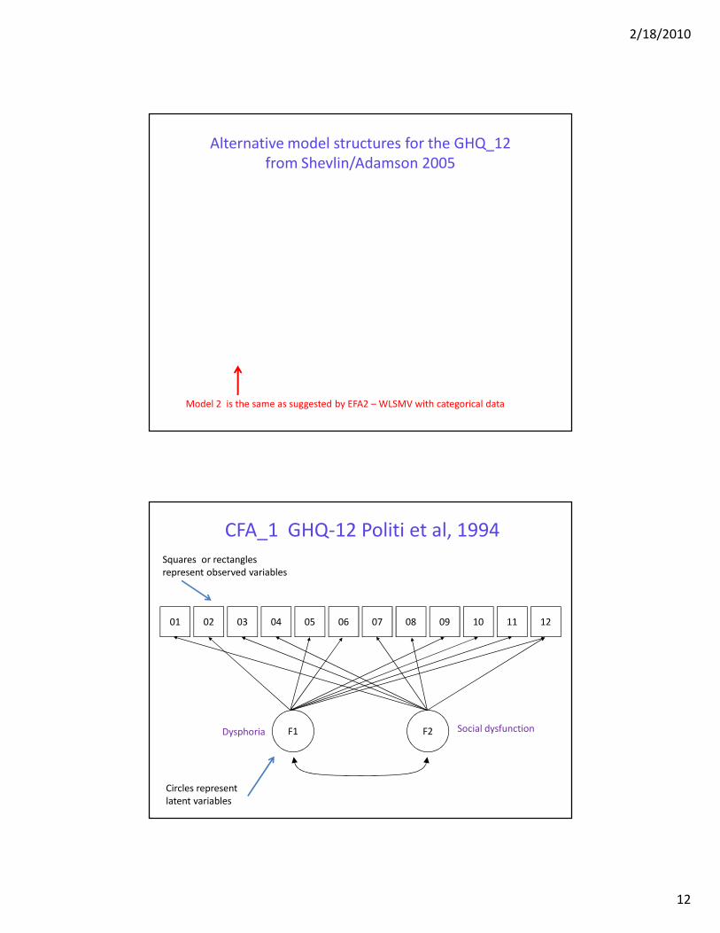
Alternative model structures for the GHQ_12

from Shevlin/Adamson 2005

Model 2 is the same as suggested by EFA2 – WLSMV with categorical data

CFA_1 GHQ-12 Politi et al, 1994

01 02 03 04 05 06 07 08 09 10 1211

F1 F2Dysphoria Social dysfunction

Circles represent

latent variables

Squares or rectangles

represent observed variables

2/18/2010

13

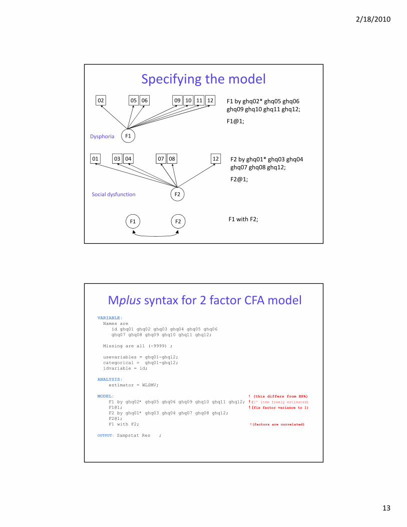
Specifying the model

02 05 06 09 10 1211

F1

01 03 04 07 08 12

F2

F1 F2

F1 by ghq02* ghq05 ghq06

ghq09 ghq10 ghq11 ghq12;

F1@1;

F2 by ghq01* ghq03 ghq04

ghq07 ghq08 ghq12;

F2@1;

F1 with F2;

Dysphoria

Social dysfunction

Mplus syntax for 2 factor CFA model

VARIABLE:

Names are

id ghq01 ghq02 ghq03 ghq04 ghq05 ghq06

ghq07 ghq08 ghq09 ghq10 ghq11 ghq12;


usevariables = ghq01-ghq12;

categorical = ghq01-ghq12;

idvariable = id;

ANALYSIS:

estimator = WLSMV;

MODEL: ! (this differs from EFA)

F1 by ghq02* ghq05 ghq06 ghq09 ghq10 ghq11 ghq12; !(1st item freely estimated)

F1@1; !(fix factor variance to 1)

F2 by ghq01* ghq03 ghq04 ghq07 ghq08 ghq12;

F2@1;

F1 with F2; !(factors are correlated)

OUTPUT: Sampstat Res ;

2/18/2010

14

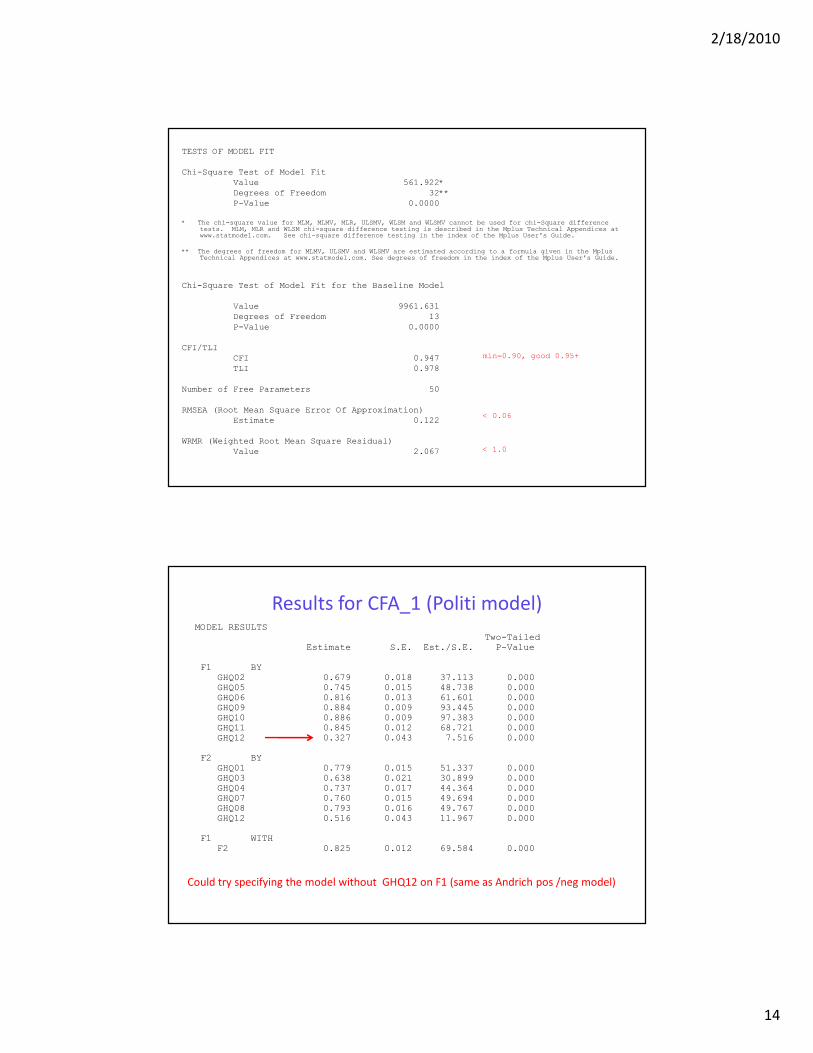
TESTS OF MODEL FIT


Value 561.922*

Degrees of Freedom 32**

P-Value 0.0000

* The chi-square value for MLM, MLMV, MLR, ULSMV, WLSM and WLSMV cannot be used for chi-Square difference tests. MLM, MLR and WLSM chi-square difference testing is described in the Mplus Technical Appendices at www.statmodel.com. See chi-square difference testing in the index of the Mplus User's Guide.

** The degrees of freedom for MLMV, ULSMV and WLSMV are estimated according to a formula given in the Mplus Technical Appendices at www.statmodel.com. See degrees of freedom in the index of the Mplus User's Guide.

Chi-Square Test of Model Fit for the Baseline Model

Value 9961.631


P-Value 0.0000

CFI/TLI

CFI 0.947

TLI 0.978

Number of Free Parameters 50

RMSEA (Root Mean Square Error Of Approximation)

Estimate 0.122

WRMR (Weighted Root Mean Square Residual)

Value 2.067

min=0.90, good 0.95+

< 0.06

< 1.0

Results for CFA_1 (Politi model)MODEL RESULTS

Two-TailedEstimate S.E. Est./S.E. P-Value

F1 BYGHQ02 0.679 0.018 37.113 0.000GHQ05 0.745 0.015 48.738 0.000GHQ06 0.816 0.013 61.601 0.000GHQ09 0.884 0.009 93.445 0.000GHQ10 0.886 0.009 97.383 0.000GHQ11 0.845 0.012 68.721 0.000GHQ12 0.327 0.043 7.516 0.000

F2 BYGHQ01 0.779 0.015 51.337 0.000GHQ03 0.638 0.021 30.899 0.000GHQ04 0.737 0.017 44.364 0.000GHQ07 0.760 0.015 49.694 0.000GHQ08 0.793 0.016 49.767 0.000GHQ12 0.516 0.043 11.967 0.000

F1 WITHF2 0.825 0.012 69.584 0.000

Could try specifying the model without GHQ12 on F1 (same as Andrich pos /neg model)

2/18/2010

15

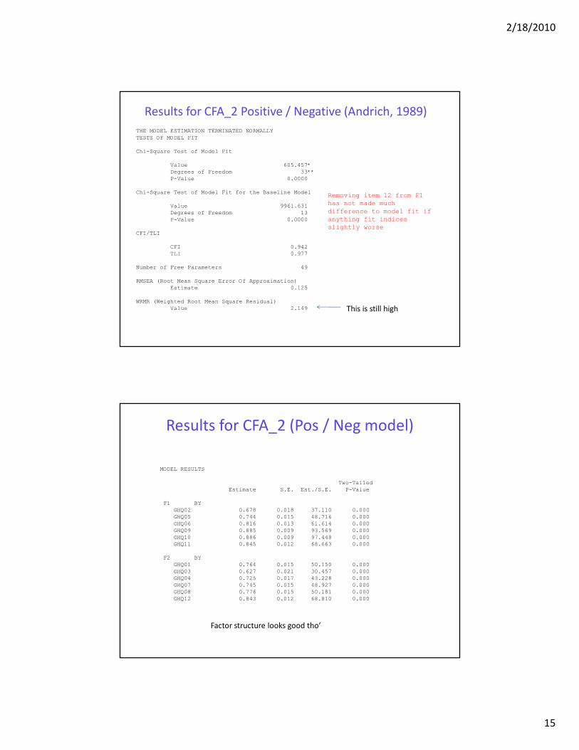
THE MODEL ESTIMATION TERMINATED NORMALLY

TESTS OF MODEL FIT


Value 605.457*


P-Value 0.0000


Value 9961.631


P-Value 0.0000

CFI/TLI

CFI 0.942

TLI 0.977



Estimate 0.125


Value 2.149

Results for CFA_2 Positive / Negative (Andrich, 1989)

Removing item 12 from F1

has not made much

difference to model fit if

anything fit indices

slightly worse

This is still high

MODEL RESULTS

Two-Tailed

Estimate S.E. Est./S.E. P-Value

F1 BY

GHQ02 0.678 0.018 37.110 0.000

GHQ05 0.744 0.015 48.716 0.000

GHQ06 0.816 0.013 61.614 0.000

GHQ09 0.885 0.009 93.569 0.000

GHQ10 0.886 0.009 97.448 0.000

GHQ11 0.845 0.012 68.663 0.000

F2 BY

GHQ01 0.764 0.015 50.150 0.000

GHQ03 0.627 0.021 30.457 0.000

GHQ04 0.725 0.017 43.228 0.000

GHQ07 0.745 0.015 48.927 0.000

GHQ08 0.776 0.015 50.181 0.000

GHQ12 0.843 0.012 68.810 0.000

Results for CFA_2 (Pos / Neg model)

Factor structure looks good tho’

2/18/2010

16

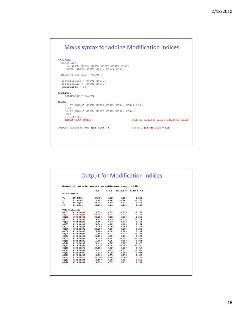
Mplus syntax for adding Modification Indices

VARIABLE:Names are



usevariables = ghq01-ghq12;categorical = ghq01-ghq12;idvariable = id;

ANALYSIS: estimator = WLSMV;

MODEL: F1 by ghq02* ghq05 ghq06 ghq09 ghq10 ghq11 ghq12; F1@1;F2 by ghq01* ghq03 ghq04 ghq07 ghq08 ghq12;F2@1;F1 with F2;ghq02 with ghq05; ! (this is needed to report modind for items)

OUTPUT: Sampstat Res Mod (10) ; ! Specify cut-off 3.84 = sig

Minimum M.I. value for printing the modification index 10.000

M.I. E.P.C. Std E.P.C. StdYX E.P.C.

BY Statements

F1 BY GHQ03 27.431 -0.299 -0.299 -0.299

F1 BY GHQ04 20.801 -0.262 -0.262 -0.262

F1 BY GHQ08 33.145 0.316 0.316 0.316

F2 BY GHQ06 23.818 0.243 0.243 0.243

WITH Statements

GHQ03 WITH GHQ02 10.770 -0.093 -0.093 -0.161

GHQ04 WITH GHQ03 133.201 0.231 0.231 0.444

GHQ05 WITH GHQ01 30.583 0.108 0.108 0.252

GHQ05 WITH GHQ03 19.834 -0.118 -0.118 -0.224

GHQ06 WITH GHQ05 13.681 0.070 0.070 0.178

GHQ07 WITH GHQ01 24.563 0.103 0.103 0.254

GHQ07 WITH GHQ05 10.709 0.069 0.069 0.156

GHQ08 WITH GHQ01 24.293 -0.107 -0.107 -0.280

GHQ08 WITH GHQ06 24.203 0.089 0.089 0.254

GHQ08 WITH GHQ07 11.508 -0.072 -0.072 -0.183

GHQ09 WITH GHQ02 20.234 0.094 0.094 0.270

GHQ09 WITH GHQ04 16.759 -0.101 -0.101 -0.321

GHQ10 WITH GHQ05 16.467 -0.087 -0.087 -0.274

GHQ10 WITH GHQ06 20.693 -0.087 -0.087 -0.326

GHQ11 WITH GHQ01 15.510 -0.093 -0.093 -0.280

GHQ11 WITH GHQ02 20.555 -0.127 -0.127 -0.317

GHQ11 WITH GHQ05 20.511 -0.112 -0.112 -0.306

GHQ11 WITH GHQ07 15.030 -0.098 -0.098 -0.284

GHQ11 WITH GHQ09 14.038 -0.076 -0.076 -0.305

GHQ11 WITH GHQ10 143.250 0.189 0.189 0.767

GHQ12 WITH GHQ04 13.509 -0.086 -0.086 -0.216

GHQ12 WITH GHQ09 15.710 0.071 0.071 0.257

Output for Modification Indices

2/18/2010

17

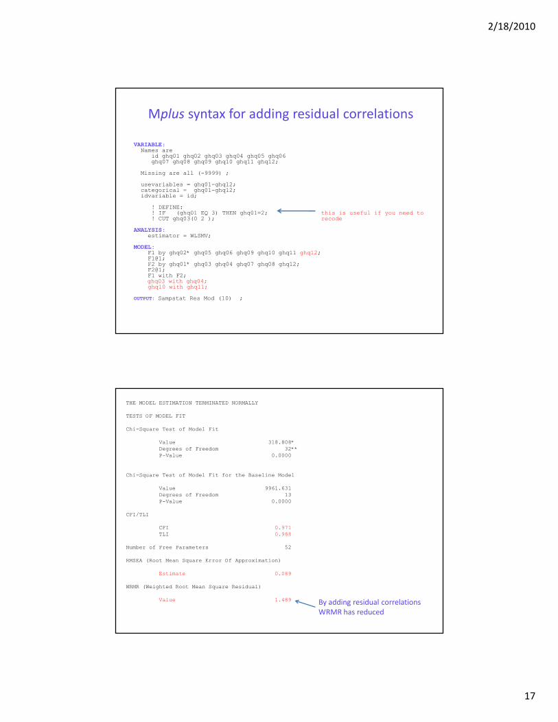
Mplus syntax for adding residual correlations

VARIABLE:Names are



usevariables = ghq01-ghq12;categorical = ghq01-ghq12;idvariable = id;

! DEFINE:! IF (ghq01 EQ 3) THEN ghq01=2; this is useful if you need to ! CUT ghq03(0 2 ); recode

ANALYSIS: estimator = WLSMV;

MODEL: F1 by ghq02* ghq05 ghq06 ghq09 ghq10 ghq11 ghq12; F1@1;F2 by ghq01* ghq03 ghq04 ghq07 ghq08 ghq12;F2@1;F1 with F2;ghq03 with ghq04;ghq10 with ghq11;

OUTPUT: Sampstat Res Mod (10) ;

THE MODEL ESTIMATION TERMINATED NORMALLY

TESTS OF MODEL FIT


Value 318.808*


P-Value 0.0000


Value 9961.631


P-Value 0.0000

CFI/TLI

CFI 0.971

TLI 0.988



Estimate 0.089


Value 1.489 By adding residual correlations

WRMR has reduced

2/18/2010

18

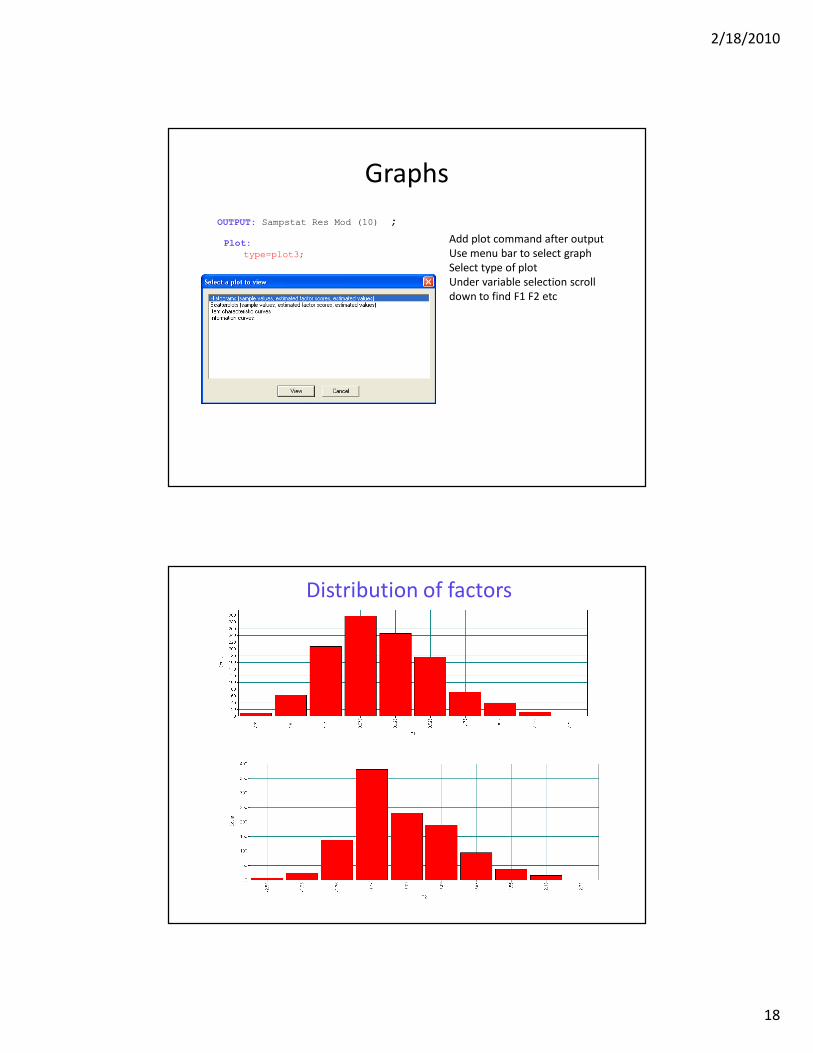
Graphs

OUTPUT: Sampstat Res Mod (10) ;

Plot:

type=plot3;

Add plot command after output

Use menu bar to select graph

Select type of plot

Under variable selection scroll

down to find F1 F2 etc

Distribution of factors

2/18/2010

19

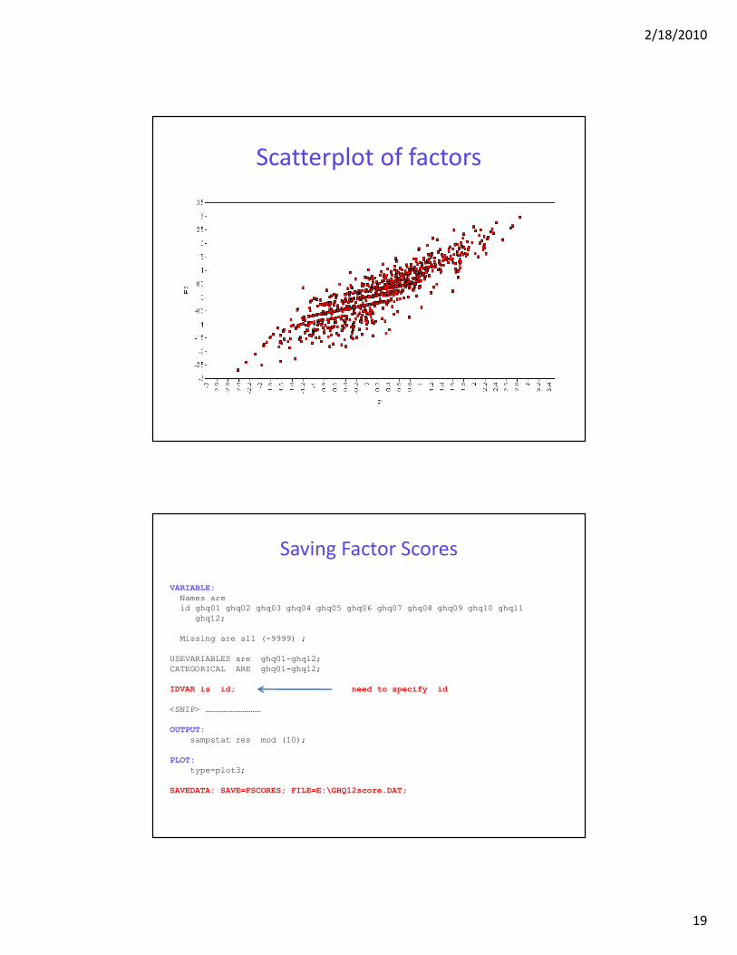
Scatterplot of factors

Saving Factor Scores

VARIABLE:

Names are


ghq12;


USEVARIABLES are ghq01-ghq12;

CATEGORICAL ARE ghq01-ghq12;

IDVAR is id; need to specify id

<SNIP> ……………………………

OUTPUT:

sampstat res mod (10);

PLOT:

type=plot3;

SAVEDATA: SAVE=FSCORES; FILE=E:\GHQ12score.DAT;

2/18/2010

20

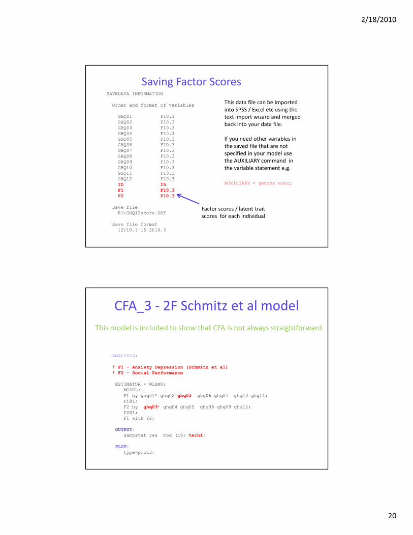
Saving Factor ScoresSAVEDATA INFORMATION

Order and format of variables

GHQ01 F10.3

GHQ02 F10.3

GHQ03 F10.3

GHQ04 F10.3

GHQ05 F10.3

GHQ06 F10.3

GHQ07 F10.3

GHQ08 F10.3

GHQ09 F10.3

GHQ10 F10.3

GHQ11 F10.3

GHQ12 F10.3

ID I5

F1 F10.3

F2 F10.3

Save file

E:\GHQ12score.DAT

Save file format

12F10.3 I5 2F10.3

This data file can be imported

into SPSS / Excel etc using the

text import wizard and merged

back into your data file.

If you need other variables in

the saved file that are not

specified in your model use

the AUXILIARY command in

the variable statement e.g.

AUXILIARY = gender educ;

Factor scores / latent trait

scores for each individual

CFA_3 - 2F Schmitz et al model

ANALYSIS:

! F1 - Anxiety Depression (Schmitz et al)

! F2 - Social Performance

ESTIMATOR = WLSMV;

MODEL:

F1 by ghq01* ghq02 ghq03 ghq06 ghq07 ghq10 ghq11;

F1@1;

F2 by ghq03* ghq04 ghq05 ghq08 ghq09 ghq12;

F2@1;

F1 with F2;

OUTPUT:

sampstat res mod (10) tech1;

PLOT:

type=plot3;

This model is included to show that CFA is not always straightforward

2/18/2010

21

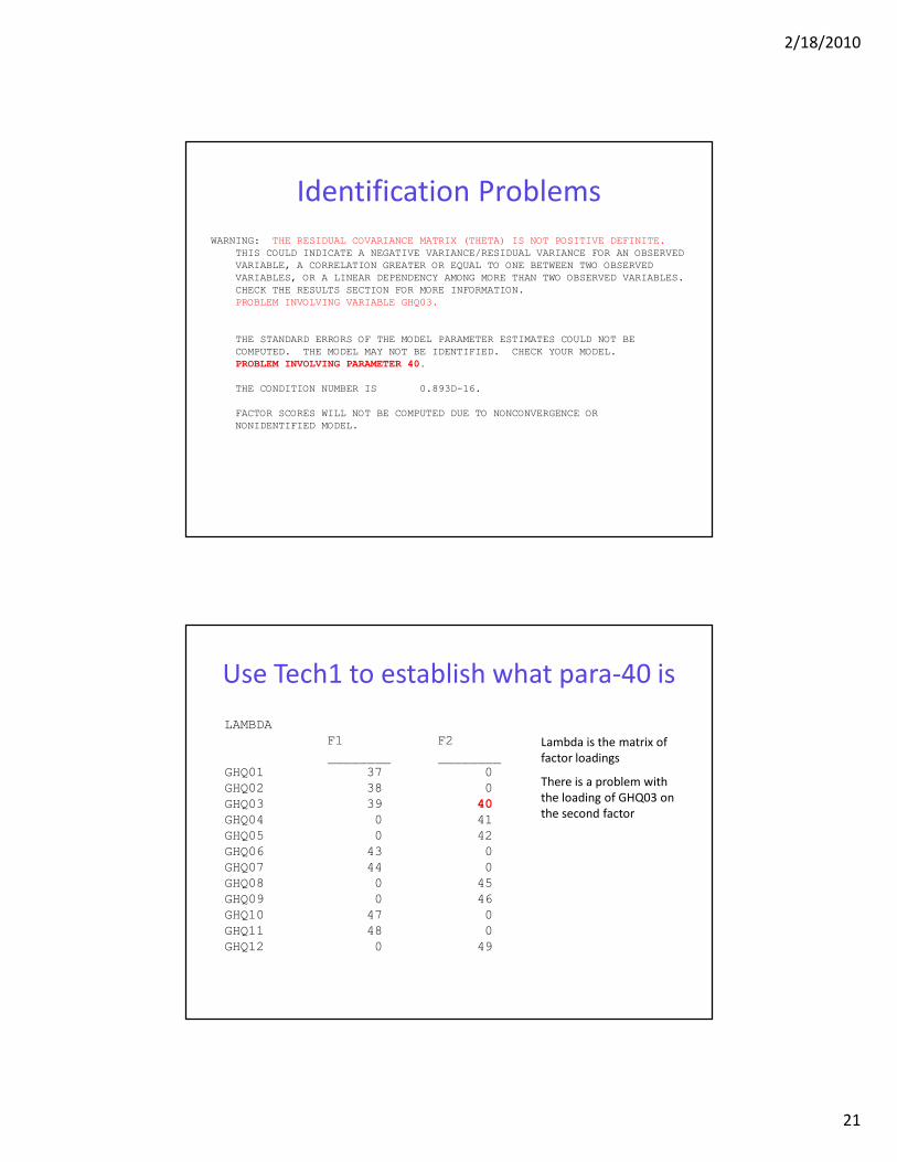
Identification Problems

WARNING: THE RESIDUAL COVARIANCE MATRIX (THETA) IS NOT POSITIVE DEFINITE.

THIS COULD INDICATE A NEGATIVE VARIANCE/RESIDUAL VARIANCE FOR AN OBSERVED

VARIABLE, A CORRELATION GREATER OR EQUAL TO ONE BETWEEN TWO OBSERVED

VARIABLES, OR A LINEAR DEPENDENCY AMONG MORE THAN TWO OBSERVED VARIABLES.

CHECK THE RESULTS SECTION FOR MORE INFORMATION.

PROBLEM INVOLVING VARIABLE GHQ03.

THE STANDARD ERRORS OF THE MODEL PARAMETER ESTIMATES COULD NOT BE

COMPUTED. THE MODEL MAY NOT BE IDENTIFIED. CHECK YOUR MODEL.

PROBLEM INVOLVING PARAMETER 40.

THE CONDITION NUMBER IS 0.893D-16.

FACTOR SCORES WILL NOT BE COMPUTED DUE TO NONCONVERGENCE OR

NONIDENTIFIED MODEL.

Use Tech1 to establish what para-40 is

LAMBDA

F1 F2

________ ________

GHQ01 37 0

GHQ02 38 0

GHQ03 39 40

GHQ04 0 41

GHQ05 0 42

GHQ06 43 0

GHQ07 44 0

GHQ08 0 45

GHQ09 0 46

GHQ10 47 0

GHQ11 48 0

GHQ12 0 49

Lambda is the matrix of

factor loadings

There is a problem with

the loading of GHQ03 on

the second factor

2/18/2010

22

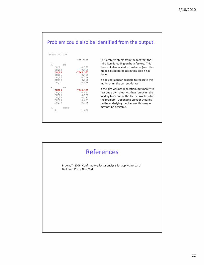
Problem could also be identified from the output:

MODEL RESULTS

Estimate

F1 BYGHQ01 0.729GHQ02 0.660GHQ03 -7545.363GHQ06 0.796GHQ07 0.714GHQ10 0.868GHQ11 0.828

F2 BYGHQ03 7545.965GHQ04 0.692GHQ05 0.721GHQ08 0.732GHQ09 0.859GHQ12 0.795

F1 WITHF2 1.000

This problem stems from the fact that the

third item is loading on both factors. This

does not always lead to problems (see other

models fitted here) but in this case it has

done.

It does not appear possible to replicate this

model using the current dataset

If the aim was not replication, but merely to

test one’s own theories, then removing the

loading from one of the factors would solve

the problem. Depending on your theories

on the underlying mechanism, this may or

may not be desirable.

References

Brown, T (2006) Confirmatory factor analysis for applied research

Guildford Press, New York

jumpstart mplus

Documents