justifying inference to the best explanation as a ...philsci-archive.pitt.edu/8821/1/ibe_gb.pdf ·...
TRANSCRIPT

Justifying Inference to the Best Explanation as a
Practical Meta-Syllogism on Dialectical Structures
Gregor Betz∗
October 1, 2011
Abstract
This article discusses how inference to the best explanation (IBE) can be
justified as a practical meta-argument. It is, firstly, justified as a practical
argument insofar as accepting the best explanation as true can be shown to
further a specific aim. And because this aim is a discursive one which propo-
nents can rationally pursue in—and relative to—a complex controversy, namely
maximising the robustness of one’s position, IBE can be conceived, secondly,
as a meta-argument. My analysis thus bears a certain analogy to Sellars’ well-
known justification of inductive reasoning [Sellars, 1969]; it is based on recently
developed theories of complex argumentation [Betz, 2010a, 2011].
1 Introduction
Inference to the best explanation (IBE) has puzzled generations of philosophers and
logicians. For, at first glance, IBEs appear to be straightforwardly fallacious. Take,
for example, the famous teleological proof for the existence of God. This argument
can be understood as an inference to the best explanation: We observe that all
subdivisions of nature are closely adjusted. The existence of God, an intelligent being
that created the universe, is presumably the best explanation of this observation.
Therefore, God exists. Yet, a simple reconstruction yields,
(A1) All subdivisions of nature are adjusted to each other such that means are
adapted to appropriate ends. (Explanandum E)
(A2) The existence of God, an intelligent being that created the universe, implies
that all subdivisions of nature are adjusted to each other such that means
are adapted to appropriate ends. (Since that hypothesis H explains E.)
(A3) Thus: God exists. (Explanans H)
By deductive standards, this argument is clearly invalid. Inference to the best
explanation seems to be, as has been widely acknowledged [e.g. Thagard, 1988,
∗Karlsruhe Institute of Technology, Germany, email: [email protected].
1

p. 140], a peculiar kind of the fallacy of affirming the consequence. However, this
sort of inference appears to be both omnipresent and reliable—not only in everyday
contexts, but in science, too.1
Let us have a brief look at premiss (A2). The reconstruction assumes that the
explanatory hypothesis H logically entails the explanandum E (possibly by making
use of some background assumptions which have been omitted). Such explanations
which can be reconstructed as valid arguments shall be called “deductive.” Ac-
cordingly, causal explanations (at least deterministic ones) and explanations that
satisfy the deductive-nomological scheme represent examples of deductive explana-
tions. (Yet, it should be noted upfront that this paper’s analysis by no means implies
that every argument satisfying the D-N scheme, let alone every deductive argument,
represents an explanation.) The overall aim of this paper is to justify inference to
the best deductive explanation (IBdE), though I shall briefly comment on statistical
explanations in the concluding section.2
The general reason why IBdE seems to be fallacious is that, in deductive rea-
soning, a statement A being a sufficient warrant for a statement B does not entail
that B is a sufficient warrant for A. We have here an asymmetry, and this asym-
metry makes IBdE a puzzle. If IBdE were, however, to be analysed in a Bayesian
framework [cf. Howson and Urbach, 2005], that puzzle would disappear. According
to Bayesian Confirmation Theory, A confirms B iff the conditional degree of belief
in B given A, P (B|A), is greater than the unconditional degree of belief in B, P (B),
i.e. iff P (B|A)/P (B) > 1. Now, a simple theorem of probability theory states that
P (B|A)/P (B) = P (A|B)/P (A). (1)
As a consequence, B confirms A if and only if A confirms B. Provided that a
deductive explanation H always confirms the explanandum E (as we have P (E|H) =
1, taking all auxiliary assumptions for granted), the explanandum E itself confirms
the explanans H. Hence, Bayesian Confirmation Theory—instead of representing a
threat to IBE, as van Fraassen [1989, pp. 160ff.] has argued—may help to justify it.
A full-fledged justification of IBdE in Bayesian terms would have to show that for
the best explanation H∗:
P (E|H∗) ≥ P (E|Hi) and P (H∗) ≥ P (Hi) (2)
1Note that inference to explanatory principles had already been at the heart of Aristotle’s phi-losophy of science [cf. Losee, 2001, chapter 1].
2The focus on deductive explanations narrows—without, however, entirely removing—the con-trast between IBE and the hypothetico-deductive account of confirmation. But unlike hypothetico-deductivism, the analysis carried out in this paper does not presuppose that some evidence Econfirms a hypothesis H if and only if H entails E.
2

for all alternative explanations Hi.3 As Hitchcock [2007] points out, that can only
be accomplished in a piecemeal fashion: It has to be shown that whatever feature
makes a hypothesis a “lovely” explanation [in the sense of Lipton, 2004] increases,
at the same time, its prior probability or the likelihood of the explanandum given
the hypothesis. This is how, within a Bayesian framework, it might be shown that
the loveliest explanation is also the likeliest.4
At first glance, this paper appears to pursue quite different a strategy for jus-
tifying IBdE. First and foremost, we don’t analyse IBdE in Bayesian terms. As a
consequence, the suggested justification of IBdE does not buy into the assumptions
and problems of Bayesian Confirmation Theory [cf. Earman, 1992, Mayo, 1996].
Whereas the general approach of this paper diverges significantly from a Bayesian
analysis, the detailed argumentation, however, will reveal close analogies to the
Bayesian reasoning I have just sketched, as will become more apparent as the argu-
ment unfolds.
The main idea of this paper can be put as follows. Accepting the loveliest ex-
planation (i.e. the one which is superior in terms of simplicity, unificatory power,
explanatory strength, etc.) as true is the best way of achieving certain intrinsic5,
epistemic aims. Thus, to the extent that these aims should be realised, it is rea-
sonable to consider the loveliest explanation as true. Accordingly, what underlies
IBdE is in fact a practical syllogism. Since both the aim as well as the appropriate
means figuring in that practical argument are evaluated with regard to our epistemic
situation, this argument can be aptly characterised as a meta-syllogism. In order
to elaborate this sketch, we have to understand more precisely (i) what exactly is
the epistemic aim which one attempts to further by accepting the best explanation
as true, (ii) why is it reasonable to pursue that aim in the first place, and (iii) why
does accepting the best explanation promote that goal. These questions make up
the overall agenda of this paper.
3Okasha [2000] claims that the loveliest explanation merely had to satisfy either P (E|H∗) ≥P (E|Hi) or P (H∗) ≥ P (Hi). But this is clearly insufficient for being the likeliest explanation sincea high likelihood might very well be offset by a low prior probability and vice versa.
4Still, Schupbach and Sprenger [2011] provide an alternative Bayesian analysis: They define aprobabilistic measure of a hypothesis’ explanatory power E and prove that E is unique with a viewto a set of conditions that spell out explanatory strength. The measure defined by Schupbach andSprenger, however, is independent of the hypothesis’ prior probability. That’s why I am doubtfulthat E may yield a full explication of inference to the best explanation (since higher prior probabilitymakes a hypothesis more lovely an explanation, or so it seems). Yet, Schupbach [2011, pp. 117-126]shows by computer simulation that the measure of explanatory power, E , is nonetheless a valuableheuristics which approximates probabilistic, Bayesian, reasoning. I take it that these results stand inno contradiction with the argumentation unfolded in this paper. With a view to future investigation,it might be worthwhile to apply and study the measure of explanatory power by Schupbach andSprenger in a dialectic framework and with a view to degrees of justification instead of degrees ofbelief.
5The rationale for an intrinsic aim does not depend on other aims. In particular, those aimswith respect to which IBdE will be justified have to be established independently of our explanatorygoals, since otherwise the justification of IBdE would obviously be trivial.
3
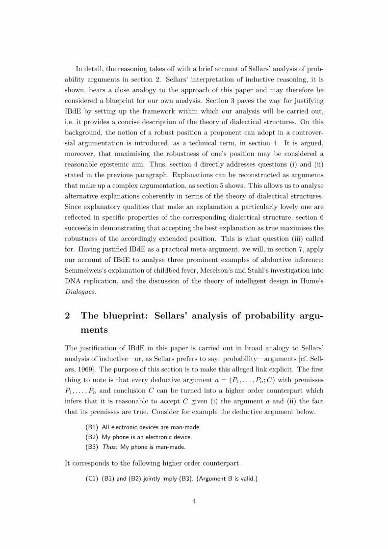
In detail, the reasoning takes off with a brief account of Sellars’ analysis of prob-
ability arguments in section 2. Sellars’ interpretation of inductive reasoning, it is
shown, bears a close analogy to the approach of this paper and may therefore be
considered a blueprint for our own analysis. Section 3 paves the way for justifying
IBdE by setting up the framework within which our analysis will be carried out,
i.e. it provides a concise description of the theory of dialectical structures. On this
background, the notion of a robust position a proponent can adopt in a controver-
sial argumentation is introduced, as a technical term, in section 4. It is argued,
moreover, that maximising the robustness of one’s position may be considered a
reasonable epistemic aim. Thus, section 4 directly addresses questions (i) and (ii)
stated in the previous paragraph. Explanations can be reconstructed as arguments
that make up a complex argumentation, as section 5 shows. This allows us to analyse
alternative explanations coherently in terms of the theory of dialectical structures.
Since explanatory qualities that make an explanation a particularly lovely one are
reflected in specific properties of the corresponding dialectical structure, section 6
succeeds in demonstrating that accepting the best explanation as true maximises the
robustness of the accordingly extended position. This is what question (iii) called
for. Having justified IBdE as a practical meta-argument, we will, in section 7, apply
our account of IBdE to analyse three prominent examples of abductive inference:
Semmelweis’s explanation of childbed fever, Meselson’s and Stahl’s investigation into
DNA replication, and the discussion of the theory of intelligent design in Hume’s
Dialogues.
2 The blueprint: Sellars’ analysis of probability argu-
ments
The justification of IBdE in this paper is carried out in broad analogy to Sellars’
analysis of inductive—or, as Sellars prefers to say: probability—arguments [cf. Sell-
ars, 1969]. The purpose of this section is to make this alleged link explicit. The first
thing to note is that every deductive argument a = (P1, . . . , Pn;C) with premisses
P1, . . . , Pn and conclusion C can be turned into a higher order counterpart which
infers that it is reasonable to accept C given (i) the argument a and (ii) the fact
that its premisses are true. Consider for example the deductive argument below.
(B1) All electronic devices are man-made.
(B2) My phone is an electronic device.
(B3) Thus: My phone is man-made.
It corresponds to the following higher order counterpart.
(C1) (B1) and (B2) jointly imply (B3). (Argument B is valid.)
4

(C2) (B1) and (B2) are true. (Its premisses are true.)
(C3) It is reasonable to accept a statement which is implied by a set of true
statements.
(C4) Thus: It is reasonable to accept (B3).
Sellars claims, I understand, that when it comes to probabilistic arguments, the
higher order counterpart is not merely a meta-reformulation of the more basic first
order argument. On the contrary, it is the meta-argument which is fundamental and
ultimately licenses inductive reasoning. The first order formulation of a probabilistic
argument merely approximates the principal and underlying higher order argument.
To illustrate this point, consider the following inductive argument.
(D1) Most professors have been abroad.
(D2) Peter is a professor.
(D3) Thus: (Probably,) Peter has been abroad.
Sellars’ analysis amounts to saying that the second order counterpart to this argu-
ment actually reads,
(E1) Most of the statements of the form “a has been abroad”, where “a” refers
to some professor, are true. (D1)
(E2) “Peter” refers to some professor. (D2)
(E3) It is, all things considered, reasonable to accept a statement which belongs
to a class of mostly true statements.
(E4) Thus: It is reasonable to accept (D3).
Interestingly, the higher order argument E does not refer to any (probabilistic)
inferential relations that are made explicit by the first order argument D. (Note
that (C1) does refer to inferential relations of argument B.) That is the reason why
Sellars can consistently suggest that the argument E is more basic than the argument
D—and not the other way around. Actually, Sellars denies that there are genuine,
independent probability arguments of the type D at all. Our inductive reasoning,
he claims, has to be reconstructed as meta-reasoning.
Both meta-arguments C and D are practical arguments. They conclude that it
is reasonable to do this or that—namely, to accept a certain statement.6 These ac-
tions are recommended with respect to a common epistemic aim. Sellars assumes—
compare premisses (C3) and (E3)—that it is reasonable to maximise the number
of true beliefs as long as the error ratio can be controlled. In regard of this epis-
temic aim, it is reasonable to accept the conclusion of a probability argument. The
6This raises the question whether we can decide (what) to believe at all. Bernard Williamsfamously answered this question in the negative [Williams, 1973]. We cannot acquire beliefs at will,he convincingly argued, because beliefs aim at truth. Admittedly, I cannot decide to believe that pwhile I am convinced that p is false. Our inability to decide to believe, however, does not underminethe practical meta-arguments we are studying presently. For these arguments try to demonstratethat adopting this or that belief is truth-conducive, or, more generally, furthers our epistemic aims.To consider such a practical meta-arguments as sound therefore doesn’t assume that we’re able toacquire arbitrary beliefs at will.
5
normative strength of probability arguments stems solely from their higher order
analysis.
Sellars’ approach may serve as a blueprint for justifying IBdE. Without attempt-
ing to impose a deductive structure, the teleological argument can be reconstructed
as,
(F1) All subdivisions of nature are adjusted to each other such that means are
adapted to appropriate ends. (Explanandum E)
(F2) The existence of God, an intelligent being that created the universe, is the
best explanation for all subdivisions of nature being adjusted to each other
such that means are adapted to appropriate ends. (Hypothesis H∗ explains
E best.)
(F3) Thus: God exists. (Explanans H∗)
I suggest that this is, like the probability argument D, not a genuine and independent
reasoning, either. What stands behind this IBdE is the following practical meta-
argument.
(G1) Accepting that God exists maximises—compared to accepting any other
alternative explanatory hypothesis—the robustness of one’s position. (Ac-
cepting the best explanation H∗ maximises the robustness of one’s position
relative to all available explanatory hypotheses.)
(G2) It is reasonable to maximise the robustness of one’s position.
(G3) One of the explanatory hypotheses should be accepted.
(G4) Thus: It is reasonable to accept that God exists.
Premiss (G1) states that accepting the best explanation is the comparatively best
way to achieve a certain epistemic aim—maximising robustness. (G2) adds that it is
reasonable to pursue that very aim while (G3) rules out the option of not accepting
any explanatory hypothesis (i.e. of being agnostic). Argument G is entirely inde-
pendent of any inferential claim contained in F. Thus, the inference expressed by F
(its normative strength) may be reduced to G in a non-circular way. Moreover, the
reconstruction of IBdE as practical meta-syllogism helps to refine the original infer-
ence pattern of IBdE. Provided the reconstruction given by G can be consistently
defended in the following sections, it demonstrates that any IBdE has to assume
that (i) H∗ is, relative to a set of alternative explanations Hi, the best explanation
of E, that (ii) E is a fact, as well as that (iii) E should be explained at all. For
unless (iii) holds, it is not clear why premiss (G3) of the second order counterpart
is true. And if the premisses of the corresponding practical meta-syllogism aren’t
true, the specific IBdE isn’t warranted in the first place.
Hence, it remains to be shown that the meta-syllogism’s premisses (G1) and
(G2) are indeed true—given the premisses of the respective first order argument.
The next section, by introducing the theory of dialectical structures, sets the stage
for doing so. Subsequently, premiss (G2) will be spelled out and justified in section 4.
6

47-2 2
13-1
65-4
8-32
110-8
7101
83
12
1412-1
-9-611
879
8
1
F/T
F/F
F/F
T/T
F/T
T/T
T/T
T/T
T/F F/T
T/F
F/F
T/T
F/F
F/F
T/T
F/F
F/T
F/T
T/F
F/F
T/T
T/F
T/F F/T
T/F
F/F
T/T
T/F
T/F
T/T
T/T
Figure 1: A dialectical structure with two complete positions attached. Truth valuesare symbolised by “T” (true) and “F” (false).
Thereupon, sections 5 and 6 explain why premiss (G1) is entailed by the premisses
of the corresponding first order IBdE.
3 The general framework: Theory of dialectical struc-
tures
A dialectical structure τ = 〈T,A,U〉 is a set of deductive arguments (premiss-
conclusion structure), T , on which an attack relation, A, and a support relation, U ,
are defined as follows (a, b ∈ T ):
• A(a, b) :⇐⇒ a’s conclusion is contradictory to one of b’s premisses;
• U(a, b) :⇐⇒ a’s conclusion is equivalent to one of b’s premisses.7
Complex debates can be reconstructed as dialectical structures. Likewise, a
reconstruction of the controversial argumentation in Part 6 of Hume’s Dialogues
Concerning Natural Religion will be sketched in section 7. Figure 1 depicts a purely
7A dialectical structures is a special type of bipolar argumentation framework as developed byCayrol and Lagasquie-Schiex [2005]. Cayrol and Lagasquie-Schiex extend the abstract approach ofDung [1995] by adding support-relations to Dung’s framework which originally considered attack-relations between arguments only. A specific interpretation of Dung’s abstract framework thatanalyses arguments as premiss-conclusion structures is carried out in Bondarenko et al. [1997]. Thetheory of dialectical structures is more thoroughly developed in Betz [2010a].
7
47-2 2
13-1
65-4
8-32
110-8
7101
83
12
1412-1
-9-611
879
8
1
F
T
F
FT
T
F
T
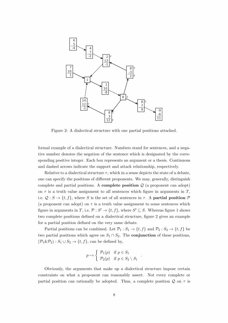
Figure 2: A dialectical structure with one partial positions attached.
formal example of a dialectical structure. Numbers stand for sentences, and a nega-
tive number denotes the negation of the sentence which is designated by the corre-
sponding positive integer. Each box represents an argument or a thesis. Continuous
and dashed arrows indicate the support and attack relationship, respectively.
Relative to a dialectical structure τ , which in a sense depicts the state of a debate,
one can specify the positions of different proponents. We may, generally, distinguish
complete and partial positions. A complete position Q (a proponent can adopt)
on τ is a truth value assignment to all sentences which figure in arguments in T ,
i.e. Q : S → {t, f}, where S is the set of all sentences in τ . A partial position P(a proponent can adopt) on τ is a truth value assignment to some sentences which
figure in arguments in T , i.e. P : S′ → {t, f}, where S′ ⊆ S. Whereas figure 1 shows
two complete positions defined on a dialectical structure, figure 2 gives an example
for a partial position defined on the very same debate.
Partial positions can be combined. Let P1 : S1 → {t, f} and P2 : S2 → {t, f} be
two partial positions which agree on S1 ∩ S2. The conjunction of these positions,
(P1&P2) : S1 ∪ S2 → {t, f}, can be defined by,
p 7→{P1(p) if p ∈ S1P2(p) if p ∈ S2 \ S1
.
Obviously, the arguments that make up a dialectical structure impose certain
constraints on what a proponent can reasonably assert. Not every complete or
partial position can rationally be adopted. Thus, a complete position Q on τ is
8
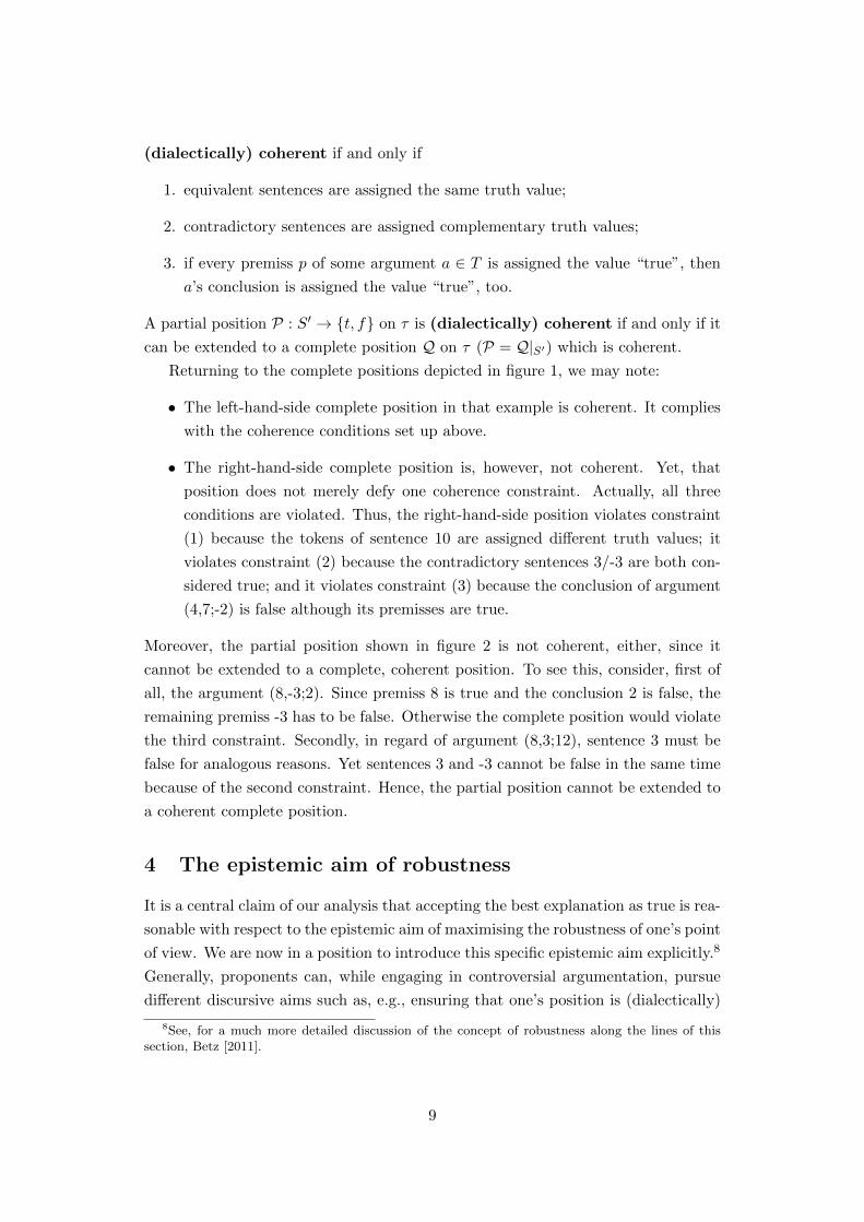
(dialectically) coherent if and only if
1. equivalent sentences are assigned the same truth value;
2. contradictory sentences are assigned complementary truth values;
3. if every premiss p of some argument a ∈ T is assigned the value “true”, then
a’s conclusion is assigned the value “true”, too.
A partial position P : S′ → {t, f} on τ is (dialectically) coherent if and only if it
can be extended to a complete position Q on τ (P = Q|S′) which is coherent.
Returning to the complete positions depicted in figure 1, we may note:
• The left-hand-side complete position in that example is coherent. It complies
with the coherence conditions set up above.
• The right-hand-side complete position is, however, not coherent. Yet, that
position does not merely defy one coherence constraint. Actually, all three
conditions are violated. Thus, the right-hand-side position violates constraint
(1) because the tokens of sentence 10 are assigned different truth values; it
violates constraint (2) because the contradictory sentences 3/-3 are both con-
sidered true; and it violates constraint (3) because the conclusion of argument
(4,7;-2) is false although its premisses are true.
Moreover, the partial position shown in figure 2 is not coherent, either, since it
cannot be extended to a complete, coherent position. To see this, consider, first of
all, the argument (8,-3;2). Since premiss 8 is true and the conclusion 2 is false, the
remaining premiss -3 has to be false. Otherwise the complete position would violate
the third constraint. Secondly, in regard of argument (8,3;12), sentence 3 must be
false for analogous reasons. Yet sentences 3 and -3 cannot be false in the same time
because of the second constraint. Hence, the partial position cannot be extended to
a coherent complete position.
4 The epistemic aim of robustness
It is a central claim of our analysis that accepting the best explanation as true is rea-
sonable with respect to the epistemic aim of maximising the robustness of one’s point
of view. We are now in a position to introduce this specific epistemic aim explicitly.8
Generally, proponents can, while engaging in controversial argumentation, pursue
different discursive aims such as, e.g., ensuring that one’s position is (dialectically)
8See, for a much more detailed discussion of the concept of robustness along the lines of thissection, Betz [2011].
9
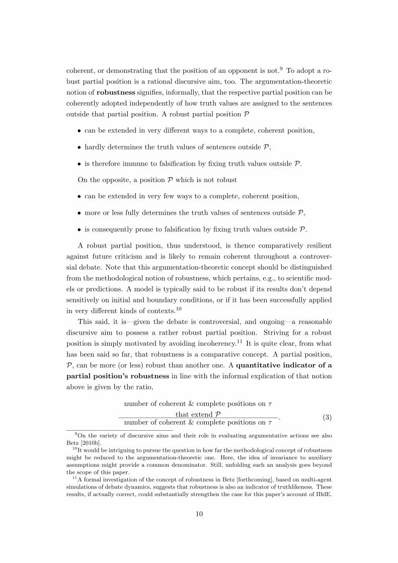
coherent, or demonstrating that the position of an opponent is not.9 To adopt a ro-
bust partial position is a rational discursive aim, too. The argumentation-theoretic
notion of robustness signifies, informally, that the respective partial position can be
coherently adopted independently of how truth values are assigned to the sentences
outside that partial position. A robust partial position P
• can be extended in very different ways to a complete, coherent position,
• hardly determines the truth values of sentences outside P,
• is therefore immune to falsification by fixing truth values outside P.
On the opposite, a position P which is not robust
• can be extended in very few ways to a complete, coherent position,
• more or less fully determines the truth values of sentences outside P,
• is consequently prone to falsification by fixing truth values outside P.
A robust partial position, thus understood, is thence comparatively resilient
against future criticism and is likely to remain coherent throughout a controver-
sial debate. Note that this argumentation-theoretic concept should be distinguished
from the methodological notion of robustness, which pertains, e.g., to scientific mod-
els or predictions. A model is typically said to be robust if its results don’t depend
sensitively on initial and boundary conditions, or if it has been successfully applied
in very different kinds of contexts.10
This said, it is—given the debate is controversial, and ongoing—a reasonable
discursive aim to possess a rather robust partial position. Striving for a robust
position is simply motivated by avoiding incoherency.11 It is quite clear, from what
has been said so far, that robustness is a comparative concept. A partial position,
P, can be more (or less) robust than another one. A quantitative indicator of a
partial position’s robustness in line with the informal explication of that notion
above is given by the ratio,
number of coherent & complete positions on τ
that extend Pnumber of coherent & complete positions on τ
. (3)
9On the variety of discursive aims and their role in evaluating argumentative actions see alsoBetz [2010b].
10It would be intriguing to pursue the question in how far the methodological concept of robustnessmight be reduced to the argumentation-theoretic one. Here, the idea of invariance to auxiliaryassumptions might provide a common denominator. Still, unfolding such an analysis goes beyondthe scope of this paper.
11A formal investigation of the concept of robustness in Betz [forthcoming], based on multi-agentsimulations of debate dynamics, suggests that robustness is also an indicator of truthlikeness. Theseresults, if actually correct, could substantially strengthen the case for this paper’s account of IBdE.
10

The concept of a position’s robustness is closely related to the notion of degree
of partial entailment. Following Wittgenstein’s basic idea in the Tractatus (and
identifying cases with complete and coherent positions on τ), the degree of partial
entailment of a partial position P1 by a partial position P2, can be defined as,
Doj(P1|P2) =number of cases with P1 & P2
number of cases with P2
=
number of complete & coherent positions that
extend P1 & P2number of complete & coherent positions that
extend P2
. (4)
Degrees of partial entailment satisfy, under certain conditions which we shall
assume to hold12, the axioms of probability theory.
Finally, the degree of justification of a partial position P can be defined as
its degree of partial entailment from the empty set,
Doj(P) = Doj(P|∅) (5)
=
number of complete & coherent positions
that extend Pnumber of complete & coherent positions
(6)
= indicator of P’s robustness. (7)
5 Reconstructing explanations as arguments in dialec-
tical structures
Explanations can be reconstructed as arguments. The explanandum, E, figures as
conclusion of the thus reconstructed explanation, the explanans, H, as one premiss
among others. This is, at least insofar as we disregard statistical explanations, a safe
assumption. It is not to be confused with the stronger claim that every argument
embodies an explanation (for its conclusion). Consider for example the explanation
of nature’s sophisticated internal adjustment by intelligent design (cf. premiss A2).
This explanation might be reconstructed as follows.
(H1) God, i.e. an intelligent being that created the universe, exists. (Central
explanatory hypothesis)
12This is the problem: For every probability measure over a set of statements, it holds thatP (A∨B) = P (A) +P (B) for contrary A,B. Now assume that the three sentences A∨B, A and Bfigure in some τ and that there is no dialectically coherent position according to which both A andB are true. Still, this does not guarantee that the (unconditional) degrees of partial entailment of Aand B add up to the (unconditional) degree of partial entailment of A∨B. That is because not everycoherent complete position according to which A is true assigns A∨B the value “true”—unless anargument like (A;A∨B) is included in τ . Thus, degrees of partial entailment satisfy the probabilityaxioms only if the respective dialectical structure is suitably augmented by simple arguments asindicated.
11
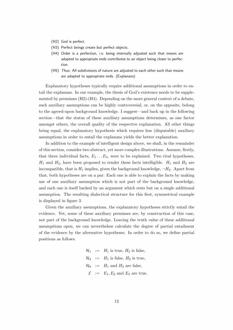
(H2) God is perfect.
(H3) Perfect beings create but perfect objects.
(H4) Order is a perfection, i.e. being internally adjusted such that means are
adapted to appropriate ends contributes to an object being closer to perfec-
tion.
(H5) Thus: All subdivisions of nature are adjusted to each other such that means
are adapted to appropriate ends. (Explanans)
Explanatory hypotheses typically require additional assumptions in order to en-
tail the explanans. In our example, the thesis of God’s existence needs to be supple-
mented by premisses (H2)-(H4). Depending on the more general context of a debate,
such auxiliary assumptions can be highly controversial, or, on the opposite, belong
to the agreed-upon background knowledge. I suggest—and back up in the following
section—that the status of these auxiliary assumptions determines, as one factor
amongst others, the overall quality of the respective explanation. All other things
being equal, the explanatory hypothesis which requires less (disputable) auxiliary
assumptions in order to entail the explanans yields the better explanation.
In addition to the example of intelligent design above, we shall, in the remainder
of this section, consider two abstract, yet more complex illustrations. Assume, firstly,
that three individual facts, E1 . . . E3, were to be explained. Two rival hypotheses,
H1 and H2, have been proposed to render these facts intelligible. H1 and H2 are
incompatible, that is H1 implies, given the background knowledge, ¬H2. Apart from
that, both hypotheses are on a par: Each one is able to explain the facts by making
use of one auxiliary assumption which is not part of the background knowledge,
and each one is itself backed by an argument which rests but on a single additional
assumption. The resulting dialectical structure for this first, symmetrical example
is displayed in figure 3.
Given the auxiliary assumptions, the explanatory hypotheses strictly entail the
evidence. Yet, some of these auxiliary premisses are, by construction of this case,
not part of the background knowledge. Leaving the truth value of these additional
assumptions open, we can nevertheless calculate the degree of partial entailment
of the evidence by the alternative hypotheses. In order to do so, we define partial
positions as follows.
H1 := H1 is true, H2 is false,
H2 := H1 is false, H2 is true,
H0 := H1 and H2 are false,
E := E1, E2 and E3 are true.
12

A6B
H2
H1B
¬H2
H2
A5B
H1
H1
E1 E2 E3
H1A1E1
H1A2E2
H2A3E2
H2A4E3
Figure 3: Dialectical structure depicting a symmetrical situation. The two explana-tory hypotheses H1 and H2 are both capable of explaining the evidence E1, ..., E3.“B” indicates statements which belong to the background knowledge and are, ac-cordingly, assumed to be true. The Ais denote auxiliary assumption which don’tbelong to the background knowledge.
This allows us to calculate the following degrees of partial entailment.13,14
Doj(E|H1) = 0.22
Doj(E|H2) = 0.22
Doj(E|H0) = 0.16
As expected, because of the symmetry, the two hypotheses entail the explanans to
the same degree. H0, which takes both hypotheses to be false, implies the evidence
E to a significantly lower degree.
Consider a further example. Now, two individual facts, E1 and E2, are to be
explained. Again, two rival, incompatible hypotheses have been proposed to explain
the evidence. While both hypotheses have a similar backing, they fare quite differ-
ently in terms of explaining E1 and E2. While H1 offers two simple explanations for
the evidence, H2 generates a rather tedious explanation for E2, and no explanation
for E1 at all. All this translates into two simple arguments for E1 and E2, both tak-
ing off at H1 and relying, on top of that, but on background assumptions. Moreover,
we have a relatively long chain of reasoning that starts from H2 and infers E2 by
using a couple of further auxiliary assumptions. Figure 4 shows the corresponding
dialectical structure.
13It is tacitly understood that all degrees of partial entailment are, in the following, calculatedrelative to the background knowledge B. So, more precisely, Doj(E|H) refers to Doj(E|H&B),and Doj(H) reads, fully spelled out, Doj(H|B), for example.
14For the numerical calculation of these as well as all degrees of justification henceforth, comparethe supplementary material.
13

A5B
H2
H1B
¬H2
H2
A4B
H1
H1
E1 E2
H1BE1
H1BE2
A2A3E2
H2A1A2
Figure 4: Dialectical structure depicting an asymmetrical situation. HypothesisH1 provides two neat explanations for the evidence. Its rival H2, however, merelyexplains E2, and this in a rather complicated or disputable way.
Once more, the rival explanatory hypotheses entail the evidence to a certain
degree. We define:
H1 := H1 is true, H2 is false,
H2 := H1 is false, H2 is true,
H0 := H1 and H2 are false,
E := E1 and E2 are true.
This allows us to calculate the following degrees of partial entailment.
Doj(E|H1) = 1
Doj(E|H2) = 0.3
Doj(E|H0) = 0.29
Hence, the hypothesis H1 strictly implies the explanans (obviously so, as the re-
constructed explanations merely rely on background assumption that are assumed
to be true). Its rival H2, however, implies the evidence E to a much lower degree.
Actually, the degree of partial entailment of the explanans by H2 is hardly higher
than by the position according to which neither hypothesis is true.
The graph-theoretical analysis of rival explanations set forth in this section ex-
hibits a structural analogy to Paul Thagard’s theory of explanatory coherence [Tha-
gard, 1992, chapter 4]. This is because Thagard, too, represents concrete explana-
tory situations as graphs which lay out the explanatory relations between different
hypotheses and items of evidence. In contrast to Thagard’s theory, however, the
approach presented in this paper doesn’t take the explanatory relations as primi-
14

tive, but reduces them to inferential relations between the respective statements so
that logico-dialectical considerations appertain to the analysis. As we will see in the
following section, this allows us to justify IBdE on argumentation-theoretic grounds.
6 Accepting the best explanation maximises robustness
This section establishes premiss (G1) of the practical meta-syllogism which under-
lies every IBdE, i.e. it demonstrates that accepting the best explanation—relative
to adopting any rival explanatory hypothesis—maximises one’s partial position’s ro-
bustness. The core of the argument can be put as follows: Assume we were to adopt
one of the alternative explanatory partial positions H1, . . . ,Hn which attempt to
explain the evidence E , thus extending our prior partial position Q. Let us denote
the background knowledge by B. Provided that the epistemic aim which guides
our choice is to maximise the robustness of our new position, we have to adopt Hk
(1 ≤ k ≤ n) such that
Doj(Hk&Q|E&B) = maxi=1...n
Doj(Hi&Q|E&B). (8)
But since we have, with Bayes’ theorem,
Doj(Hi&Q|E&B) = Doj(Hi|E&B&Q)×Doj(Q|E&B)︸ ︷︷ ︸const.
∝ Doj(E|Hi&B&Q)×Doj(Hi|B&Q)
Doj(E|B&Q)︸ ︷︷ ︸const.
∝ Doj(E|Hi&B&Q)×Doj(Hi|B&Q), (9)
it remains but to be shown that the product in equation 9 is maximal for the best
explanation.
The argument in the remainder of this section proceeds, generally spoken, in
four steps: First, we spell out the comparative concept of a better (“lovelier”) ex-
planation. Secondly, we show that whatever contributes to some hypothesis H1
being a better explanation than H2 is reflected in certain features of the dialecti-
cal structure that reconstructs the respective explanations. Thirdly, we argue that
these features increase either the likelihood of the evidence given the hypothesis,
Doj(E|Hi&B&Q), or the prior degree of justification of the respective hypothesis,
Doj(Hi|B&Q). So we can, finally, conclude that the best explanation maximises
the enlarged position’s robustness, indeed.
This general reasoning has to be carried out in a piecemeal fashion. Thus we
identify, in the following, different explanatory qualities which characterise a good
explanation and demonstrate for each of these how they increase either the likeli-
15

hood of the evidence given the hypothesis or the prior degree of justification of the
respective hypothesis.
Scope. If H1 explains more pieces of evidence than H2, then H1 is ceteris paribus
a better explanation than H2. What does this mean in terms of the recon-
structed dialectical structure? Assume that H1 explains E1, . . . , En whereas
H2 explains but E1, . . . , Em with n > m. Let each individual explanation rely
on one disputable auxiliary assumption. So we have n arguments starting from
H1 and m arguments with premiss H2. But then, as is intuitively clear, the
total evidence E (including E1, . . . , En) is entailed by H1 to a higher degree
than by H2.15 Hence Doj(E|H1&B&Q) > Doj(E|H2&B&Q).
Precision. If H1 explains the same phenomena as H2, yet with a much higher
degree of precision, then H1 is ceteris paribus a better explanation than H2.
This situation may be reconstructed as follows. Let E1 and E2 state two facts
about one and the same phenomenon. H1 explains E1; H2 explains E2. But
assume that E1 is a much more detailed and specific statement than E2. As
a consequence, E1 entails (given appropriate background assumptions) E2.
Therefore, H1 partially entails (and explains) both pieces of evidence whereas
H2 merely explains one. H1 is thus superior in terms of scope and, according
to the previous point, we thence have Doj(E|H1&B&Q) > Doj(E|H2&B&Q).
Simplicity. If the explanations based on H1 are simpler than those based on H2,
H1 is ceteris paribus a better explanation than H2. An explanation is simple,
if it relies on few auxiliary assumptions; it is, on the contrary, complicated, if
many disputable assumptions are involved.16 This characteristic, it seems to
me, is straightforwardly translated into the number of auxiliary assumptions
the reconstruction of an explanation has to make use of. Thus, the simpler an
explanation, the fewer disputable premisses figure in its reconstruction (cf. the
example given in figure 4.). Consequently, an explanatory hypothesis which
gives rise to a simpler explanation entails the explanandum, ceteris paribus, to
a higher degree. Therefore, Doj(E|H1&B&Q) > Doj(E|H2&B&Q).
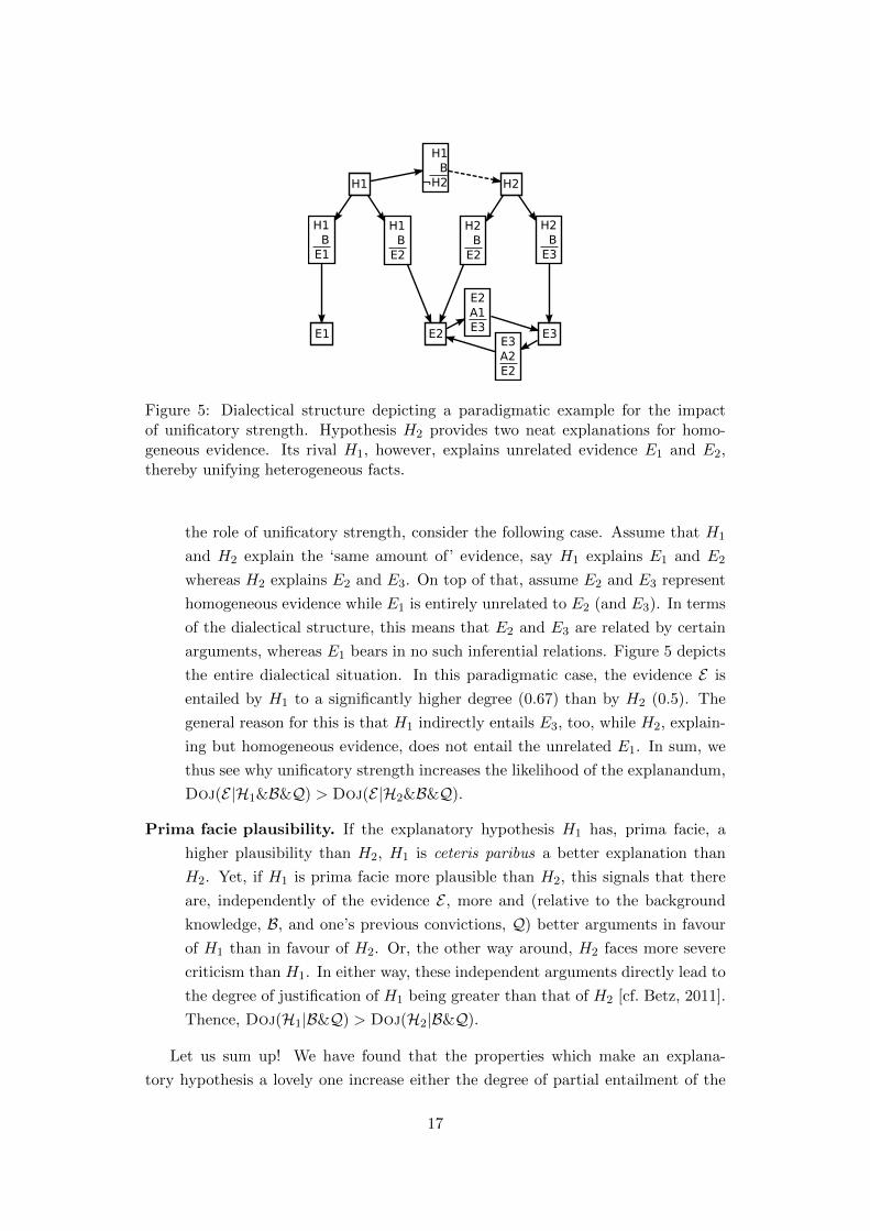
Unificatory strength. If H2 explains closely related and homogeneous pieces of
evidence, whereas H1 can explain previously unrelated and heterogeneous ev-
idence, H1 is ceteris paribus a better explanation than H2. To understand
15To make this more explicit, note that the number of complete and coherent positions thatextend E&H1 equals the number of those positions that extend E&H2. So the likelihood merelydepends on the number of positions which extend the respective hypotheses (see equation 4). Butbecause the reconstructed explanations impose n constraints on H1 but only m < n constraints onH2, strictly more positions extend H2 than H1. Thus Doj(E|H1) > Doj(E|H2).
16Note that the simplicity of an explanation should be distinguished from the simplicity of theexplanatory hypothesis on which the explanation is based.
16
E3A2E2
H1B
¬H2 H2
E2A1E3
H1
E1 E2 E3
H1BE1
H1BE2
H2BE2
H2BE3
Figure 5: Dialectical structure depicting a paradigmatic example for the impactof unificatory strength. Hypothesis H2 provides two neat explanations for homo-geneous evidence. Its rival H1, however, explains unrelated evidence E1 and E2,thereby unifying heterogeneous facts.
the role of unificatory strength, consider the following case. Assume that H1
and H2 explain the ‘same amount of’ evidence, say H1 explains E1 and E2
whereas H2 explains E2 and E3. On top of that, assume E2 and E3 represent
homogeneous evidence while E1 is entirely unrelated to E2 (and E3). In terms
of the dialectical structure, this means that E2 and E3 are related by certain
arguments, whereas E1 bears in no such inferential relations. Figure 5 depicts
the entire dialectical situation. In this paradigmatic case, the evidence E is
entailed by H1 to a significantly higher degree (0.67) than by H2 (0.5). The
general reason for this is that H1 indirectly entails E3, too, while H2, explain-
ing but homogeneous evidence, does not entail the unrelated E1. In sum, we
thus see why unificatory strength increases the likelihood of the explanandum,
Doj(E|H1&B&Q) > Doj(E|H2&B&Q).
Prima facie plausibility. If the explanatory hypothesis H1 has, prima facie, a
higher plausibility than H2, H1 is ceteris paribus a better explanation than
H2. Yet, if H1 is prima facie more plausible than H2, this signals that there
are, independently of the evidence E , more and (relative to the background
knowledge, B, and one’s previous convictions, Q) better arguments in favour
of H1 than in favour of H2. Or, the other way around, H2 faces more severe
criticism than H1. In either way, these independent arguments directly lead to
the degree of justification of H1 being greater than that of H2 [cf. Betz, 2011].
Thence, Doj(H1|B&Q) > Doj(H2|B&Q).
Let us sum up! We have found that the properties which make an explana-
tory hypothesis a lovely one increase either the degree of partial entailment of the
17

Doj(E|Hi) × Doj(Hi) ∝ Doj(Hi|E)
i=1 0.22 0.35 0.4i=2 0.22 0.35 0.4i=0 0.16 0.31 0.2
Table 1: Degrees of partial entailment for the dialectical structure shown in figure 3.
Doj(E|Hi) × Doj(Hi) ∝ Doj(Hi|E)
i=1 1 0.19 0.44i=2 0.3 0.48 0.33i=0 0.29 0.33 0.22
Table 2: Degrees of partial entailment for the dialectical structure shown in figure 4.
explanandum by the hypothesis, Doj(E|Hi&B&Q), or the degree of justification
of the hypothesis itself, Doj(Hi|B&Q). This seems to provide sufficient reason to
stipulate that some H1 constitutes a strictly better explanation than H2 iff H1 max-
imises the product of those two terms. Note that such an explication of the notion of
the best explanation allows for weighing the different explanatory qualities against
each other: E.g., if some hypothesis H1 substantially surpasses H2 with respect to
scope, precision, and unificatory strength while being only slightly inferior in terms
of prima facie plausibility, H1 obviously counts as the lovelier explanation—and this
corresponds to the fact that the product of Doj(E|Hi&B&Q) and Doj(Hi|B&Q) is
greater for H1 than for H2. As an immediate consequence, the best explanation—
call it H∗—of a set of alternative hypotheses thus satisfies equation 8. As we have
seen, this means that adopting the best explanation maximises the robustness of
one’s (extended) position. Thence, we have justified the general premiss (G1) of
the practical meta-argument which underlies every inference to the best (deductive)
explanation.
Let us apply these findings to the formal examples we have studied in the previous
section. Consider the case of the two symmetric explanations depicted in figure 3.
Table 1 details the degrees of partial entailment of the respective partial positions.
As the last column shows, extending one’s initial partial position by H1 yields as
robust a new position as accepting H2. In regard of the symmetry between the
explanatory hypothesis, this is not surprising. We see, moreover, that enlarging
one’s position by assigning both hypotheses the truth-value “false”, H3, results in
a significantly less robust position. With a view to maximising robustness, one of
the two equally lovely explanations should be accepted. Let us turn to the second,
asymmetric example displayed in figure 4. Table 2 reports the corresponding degrees
of partial entailment. We had previously assumed that in this example, H1 clearly
provides the better explanation. This is reflected in the degree of partial entailment
of the evidence. Still, in terms of unconditional degree of justification, H1 appears to
18

be worse off than H2 (0.19 vs. 0.48).17 This relative shortcoming of H1 is, however,
outweighed by its success in entailing the explanandum, as the last column shows.
Accepting H1 (instead of H2) as true, maximises the robustness of the accordingly
extended position. Moreover, considering both hypotheses as false would be the
worst thing to do with regard to fostering robustness. Inference to the best deductive
explanation, i.e. to H1, is justified in this second example, too.
7 Applying the account
7.1 Semmelweis’s explanation of childbed fever
Ignaz Semmelweis’s investigation into the causes of childbed fever in the mid 19th
century has been prominently used as a case study in philosophy of science [Hempel,
1966, pp. 3-8]. Here, I follow closely Lipton’s analysis of this example [Lipton, 2004,
pp. 74ff.] in order to show that Semmelweis’s abductive inferences can be justified
in line with the dialectic account of IBdE set forth in this paper.
Comparing two maternity divisions in his Viennese hospital, Semmelweis ob-
served that the proportion of women who contracted childbed fever varied substan-
tially between the two groups. This represented the main observation Semmelweis
tried to understand.
(E1) More women contract childbed fever in the first than in the second division.
Semmelweis considered three types of hypotheses that presumably identify causes
of childbed fever. The hypotheses of the first type suggest causes that actually didn’t
vary between the two divisions, such as, e.g., epidemic influences, which would effect
entire city districts in similar ways,
(EP) The outbreak of childbed fever is controlled by epidemic influences.
This hypothesis, however, neither explained the observed differences (E1), nor
were its particular observational implications, such as variations between different
hospitals (we abbreviate: E5, E6), verified by Semmelweis.
In contrast, the hypotheses of the second type do refer to certain differences
between the two divisions. But Semmelweis judged that the specific differences
17This is, to a certain degree, an artificial effect due to the tightly restricted example. Thearguments which primarily determine, according to our example, the degrees of justification arethe reconstructed explanations themselves. Yet, every observational implication of a hypothesisrepresents eo ipso a potential counter-argument and thus reduces, according to the dialecticalanalysis, its unconditional degree of justification. In a dialectical structure which consists mainly ofthe reconstructed explanations, the explanatory hypothesis with the greater scope, precision, andunificatory strengths will therefore necessarily possess the lower prima facie degree of justification.This effect would, however, vanish if a sufficiently large part of the entire debate were reconstructedsuch that arguments which are independent of the explanandum E dominated the unconditionaldegrees of justification.
19
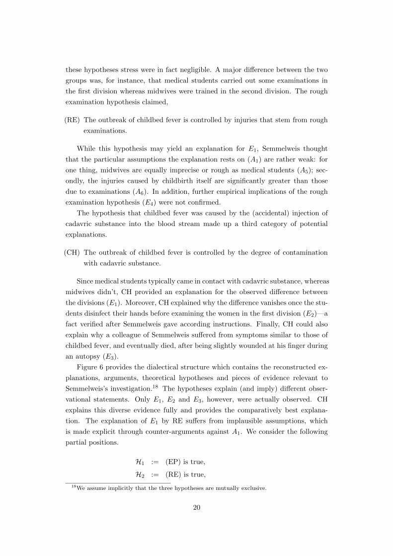
these hypotheses stress were in fact negligible. A major difference between the two
groups was, for instance, that medical students carried out some examinations in
the first division whereas midwives were trained in the second division. The rough
examination hypothesis claimed,
(RE) The outbreak of childbed fever is controlled by injuries that stem from rough
examinations.
While this hypothesis may yield an explanation for E1, Semmelweis thought
that the particular assumptions the explanation rests on (A1) are rather weak: for
one thing, midwives are equally imprecise or rough as medical students (A5); sec-
ondly, the injuries caused by childbirth itself are significantly greater than those
due to examinations (A6). In addition, further empirical implications of the rough
examination hypothesis (E4) were not confirmed.
The hypothesis that childbed fever was caused by the (accidental) injection of
cadavric substance into the blood stream made up a third category of potential
explanations.
(CH) The outbreak of childbed fever is controlled by the degree of contamination
with cadavric substance.
Since medical students typically came in contact with cadavric substance, whereas
midwives didn’t, CH provided an explanation for the observed difference between
the divisions (E1). Moreover, CH explained why the difference vanishes once the stu-
dents disinfect their hands before examining the women in the first division (E2)—a
fact verified after Semmelweis gave according instructions. Finally, CH could also
explain why a colleague of Semmelweis suffered from symptoms similar to those of
childbed fever, and eventually died, after being slightly wounded at his finger during
an autopsy (E3).
Figure 6 provides the dialectical structure which contains the reconstructed ex-
planations, arguments, theoretical hypotheses and pieces of evidence relevant to
Semmelweis’s investigation.18 The hypotheses explain (and imply) different obser-
vational statements. Only E1, E2 and E3, however, were actually observed. CH
explains this diverse evidence fully and provides the comparatively best explana-
tion. The explanation of E1 by RE suffers from implausible assumptions, which
is made explicit through counter-arguments against A1. We consider the following
partial positions.
H1 := (EP) is true,
H2 := (RE) is true,
18We assume implicitly that the three hypotheses are mutually exclusive.
20
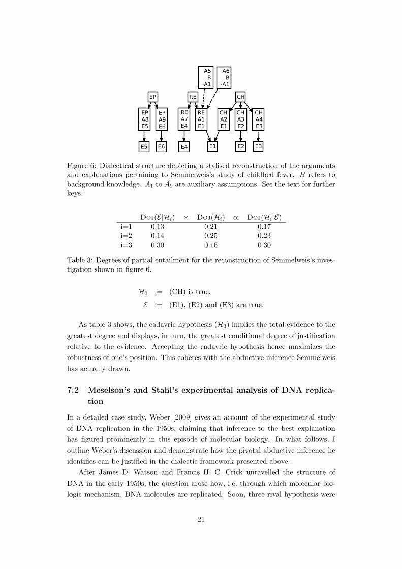
REA1E1
CHA3E2
CHA2E1
A6B
¬A1
E2E1
CH
E3
EP
A5B
¬A1
RE
CHA4E3
E5 E6 E4
REA7E4
EPA9E6
EPA8E5
Figure 6: Dialectical structure depicting a stylised reconstruction of the argumentsand explanations pertaining to Semmelweis’s study of childbed fever. B refers tobackground knowledge. A1 to A9 are auxiliary assumptions. See the text for furtherkeys.
Doj(E|Hi) × Doj(Hi) ∝ Doj(Hi|E)
i=1 0.13 0.21 0.17i=2 0.14 0.25 0.23i=3 0.30 0.16 0.30
Table 3: Degrees of partial entailment for the reconstruction of Semmelweis’s inves-tigation shown in figure 6.
H3 := (CH) is true,
E := (E1), (E2) and (E3) are true.
As table 3 shows, the cadavric hypothesis (H3) implies the total evidence to the
greatest degree and displays, in turn, the greatest conditional degree of justification
relative to the evidence. Accepting the cadavric hypothesis hence maximizes the
robustness of one’s position. This coheres with the abductive inference Semmelweis
has actually drawn.
7.2 Meselson’s and Stahl’s experimental analysis of DNA replica-
tion
In a detailed case study, Weber [2009] gives an account of the experimental study
of DNA replication in the 1950s, claiming that inference to the best explanation
has figured prominently in this episode of molecular biology. In what follows, I
outline Weber’s discussion and demonstrate how the pivotal abductive inference he
identifies can be justified in the dialectic framework presented above.
After James D. Watson and Francis H. C. Crick unravelled the structure of
DNA in the early 1950s, the question arose how, i.e. through which molecular bio-
logic mechanism, DNA molecules are replicated. Soon, three rival hypothesis were
21

proposed that described different replication mechanisms.
According to the semi-conservative replication hypothesis (SC), originally sug-
gested by Watson and Crick, the two (identical) strands of a DNA molecule are
separated before both strands serve as blueprints to synthesize further, identical
strands. Each old strand pairs up with a newly synthesized one to form, finally, a
new DNA molecule.
Max Delbruck, doubtful that DNA molecules can be efficiently unravelled, pro-
posed an alternative replication mechanism: so-called dispersive replication (DI). He
suggested that DNA strands be synthesized section-wise, whereas newly synthesized
and old DNA sections are alternately conjoined to form replicated molecules.
A third mechanism has been described by Gunther Stent. According to the
conservative hypothesis (CO), DNA molecules are fully left intact (their two strands
are neither separated nor cut and re-conjoined) when being copied.
In 1957, Matthew Meselson and Frank Stahl conducted an experiment in order to
investigate DNA replication. They grew microorganisms under different, controlled
conditions. Bacteria, when reproducing, use the atomic material available in their
environment so as to build new DNA. Meselson and Stahl systematically varied this
environment, and the available material that serves as building blocks for new DNA.
Specifically, they made two different isotypes of nitrogen (i.e. with different weight)
available to the microorganisms, who first grew in an environment with light and
then continued to reproduce in an environment with heavy nitrogen. After switching
to the new medium with heavy nitrogen, Meselson and Stahl determined the weight
of the DNA molecules at regular intervals by using high precision centrifuges. They
found DNA molecules whose weight was exactly in between that of DNA which is
merely composed of heavy nitrogen and that of DNA which comprises only light
nitrogen. Moreover, the weight of DNA molecules didn’t vary as the bacteria con-
tinued to multiply in the new medium with heavy nitrogen. These data patterns
represent the main evidence (E) to be explained.
Weber stresses, in his discussion of the experiment, that the semi-conservative
hypothesis yields a straight-forward explanation for this observation. Together with
the experimental mechanism (EM), which consists in background knowledge and a
key assumption about the functioning of the measurement process (A1), SC implies
the data patterns (E). This is not true for the alternative hypotheses. In contrast,
Weber claims, they imply non-E given the experimental set-up. Only by denying
the auxiliary assumption A1 can the dispersive and the conservative hypothesis be
made consistent with the evidence. (This possibility is also the reason why the entire
inference does not simply consist in refuting rival hypotheses.) Moreover, only by
presuming additional auxiliary assumptions which are not part of the experimental
set-up (A2 respectively A3) do DI and CO provide explanations for the evidence.
22
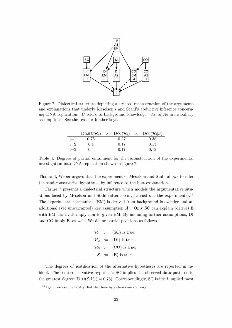
SCEME
DIA2E
BA1EM
COEM¬E
E
DI CO
DIEM¬E
SC
COA3E
Figure 7: Dialectical structure depicting a stylised reconstruction of the argumentsand explanations that underly Meselson’s and Stahl’s abductive inference concern-ing DNA replication. B refers to background knowledge. A1 to A3 are auxiliaryassumptions. See the text for further keys.
Doj(E|Hi) × Doj(Hi) ∝ Doj(Hi|E)
i=1 0.75 0.27 0.38i=2 0.4 0.17 0.13i=3 0.4 0.17 0.13
Table 4: Degrees of partial entailment for the reconstruction of the experimentalinvestigation into DNA replication shown in figure 7.
This said, Weber argues that the experiment of Meselson and Stahl allows to infer
the semi-conservative hypothesis by inference to the best explanation.
Figure 7 presents a dialectical structure which models the argumentative situ-
ations faced by Meselson and Stahl (after having carried out the experiments).19
The experimental mechanism (EM) is derived from background knowledge and an
additional (yet unwarranted) key assumption A1. Only SC can explain (derive) E
with EM. Its rivals imply non-E, given EM. By assuming further assumptions, DI
and CO imply E, as well. We define partial positions as follows.
H1 := (SC) is true,
H2 := (DI) is true,
H3 := (CO) is true,
E := (E) is true.
The degrees of justification of the alternative hypotheses are reported in ta-
ble 4. The semi-conservative hypothesis SC implies the observed data patterns to
the greatest degree (Doj(E|H1) = 0.75). Correspondingly, SC is itself implied most
19Again, we assume tacitly that the three hypotheses are contrary.
23

strongly by the evidence. Hence, assenting to the loveliest explanation, SC, maxi-
mizes robustness. This justifies the abductive inference that led to the acceptance
of the semi-conservative replication hypothesis in molecular biology.
7.3 Hume’s critique of intelligent design
The Dialogues Concerning Natural Religion [Hume, 1935] dissect the theory of in-
telligent design and deliver a trenchant criticism of what Kant later called the tele-
ological proof of the existence of God. As indicated in the introductory section,
the teleological proof may be understood as an inference to the best explanation.
Hume’s critique of this very argument in Part 6 of the Dialogues shall serve as a
final test case for our analysis of IBdE.
The Dialogues are, on the whole, concerned with the question how to explain a
specific piece of evidence. Namely,
(E1) All subdivisions of nature are adjusted to each other such that means are
adapted to appropriate ends.
In Part 6, particular attention is paid to an additional fact,
(E2) Nature is a dynamic system characterised by: A continual circulation of matter
which produces no disorder; the conservation of matter; the operation of each
subdivision so as to preserve both itself as well as the whole.
The hypothesis of intelligent design is put forward, in Part 2, to explain the evidence
E1.
(ID) Hypothesis of intelligent design: God, i.e. an intelligent, omniscient and almighty
being, has created the universe.
Hume seeks to undermine, in Part 6, the (abductive) inference to ID by proposing
alternative explanatory hypotheses which explain the available evidence at least as
good as ID, if not strictly better. Accordingly, Hume suggests that the evidence E2,
which is, he contends, only vaguely explained by the assumption that God created
the universe, could equally be explained by the hypothesis that God is the soul of
the world.
(SW) Hypothesis of Deity as the soul of the world: The universe resembles an animal,
and God is its soul, the soul of the world.
The hypotheses ID and SW, excluding each other, represent incompatible rivals. A
third explanatory hypothesis, introduced in Part 6, reads,
(IO) Hypothesis of immanent order: Nature possesses an immanent or inherent
tendency to self-organisation.
24

Figure 8: Dialectical structure depicting a stylised reconstruction of Part 6 of Hume’sDialogues. B refers to background knowledge. A1 and A2 are auxiliary assumptions.See the text for further keys.
Hume claims that IO is sufficiently powerful to explain both pieces of evidence E1
and E2. On top of that, he maintains that the two hypotheses ID and SW presuppose
the existence of some immanent tendency to self-organisation and therefore entail
IO anyway. This said, IO has the widest explanatory scope and is prima facie no less
plausible than its rivals (for being presupposed by them). Intuitively, IO therefore
yields the loveliest explanation of the evidence. Let us see whether this is reflected
in an analysis along the lines of this paper. Assuming, for the sake of simplicity,
that all the auxiliary assumptions involved in the explanations just sketched belong
to the background knowledge, we may reconstruct the dialectical structure as shown
in figure 8.20 We shall define partial positions as follows.
H1 := (ID) is true,
H2 := (SW) is true,
H3 := (IO) is true,
E := (E1) and (E2) are true.
Table 5 displays the resulting degrees of partial entailment. The principle of
immanent order (IO) surpasses its rival hypotheses both in terms of degree of partial
entailment of the evidence as well as in terms of unconditional degree of justification.
Moreover, IO is implied twice as strongly by the evidence as its rivals. Therefore,
extending the initial position (B) by IO results in an enlarged position which is
20A much more detailed reconstruction can be found in Betz [2010a, appendix C].
25

Doj(E|Hi) × Doj(Hi) ∝ Doj(Hi|E)
i=1 0.75 0.22 0.3i=2 0.75 0.22 0.3i=3 1 0.33 0.6
Table 5: Degrees of partial entailment for the reconstruction of Hume’s Dialoguesshown in figure 8.
more robust than the position augmented by ID or SW. This immediately blocks
any inference to the thesis of intelligent design by IBdE. Hume’s critique of the
teleological argument succeeds. If the evidence E1 and E2 were to be explained
at all—what Hume, by the way, doubts—and one of the alternative explanatory
hypotheses should consequently be adopted, if, in other words, the specific instance
of the general premiss (G3) were true in this case, then accepting IO, not ID, would
be the reasonable thing to do.
8 Conclusion
We have argued that IBdEs can be reconstructed as practical meta-syllogisms,
(I1) Accepting the best explanation H∗ maximises the robustness of one’s posi-
tion relative to accepting any other available explanatory hypothesis.
(I2) It is reasonable to maximise the robustness of one’s position.
(I3) One of the explanatory hypotheses should be accepted.
(I4) Thus: It is reasonable to accept H∗.
The first premiss (I1) of such an argument has to be evaluated with respect to a
certain state of debate being represented by a dialectical structure. This dialectical
structure includes, amongst further arguments, the reconstructed explanations. We
have argued, moreover, that the second premiss (I2) holds universally. The third
premiss (I3), however, is clearly case sensitive and requires specific attention. If
a proponent denies that any explanatory hypothesis should be adopted at all, e.g.
because she prefers to remain agnostic and doesn’t feel that certain evidence is
in urgent need of explanation, she has successfully blocked the IBdE. The meta-
argument represented by scheme (I) corresponds to the following first order scheme,
(J1) The explanatory hypothesis H∗ provides, relative to any other available
explanatory hypothesis, the best explanation for some evidence E.
(J2) E is the case.
(J3) E ought to be explained.
(J4) Thus: H∗.
Premisses (J1) and (J2) entail premiss (I1) of the meta-argument. Premiss (J3)
implies (I3). Thus, we have been able to justify IBdE. In the same time, our anal-
ysis has, however, exposed the weak links of IBdE, explaining why this kind of
26
reasoning is by and large much less compelling than a sound deductive argument:
First of all, it is only reasonable to extend one’s position in the most robust way
if specific, contestable assumptions are satisfied (cf. J3/I3). In addition, the most
robust extension of one’s position may still turn out to be false—either because the
true hypothesis did not even figure among the alternative explanations, or because
an explanatory hypothesis which exhibits a low prima facie plausibility and which
hardly explains the evidence turns out to be correct in the long run. In addition to
explaining the relative weakness of IBdE, we can account, by reconstructing IBdE
as a meta-argument, for IBdE’s non-monotonicity. This is because a change of the
background knowledge, or the introduction of new arguments alters the dialectical
structure with regard to which the premisses of an IBdE are evaluated. As a conse-
quence, the hypothesis that displayed, previously, the highest robustness and that
is referred to in premiss (I1) might not do so any more once additional knowledge
has been acquired.
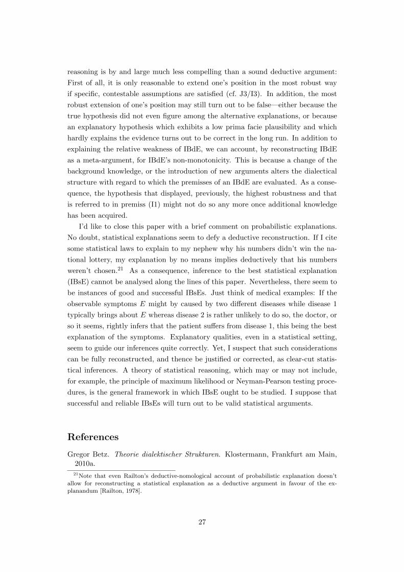
I’d like to close this paper with a brief comment on probabilistic explanations.
No doubt, statistical explanations seem to defy a deductive reconstruction. If I cite
some statistical laws to explain to my nephew why his numbers didn’t win the na-
tional lottery, my explanation by no means implies deductively that his numbers
weren’t chosen.21 As a consequence, inference to the best statistical explanation
(IBsE) cannot be analysed along the lines of this paper. Nevertheless, there seem to
be instances of good and successful IBsEs. Just think of medical examples: If the
observable symptoms E might by caused by two different diseases while disease 1
typically brings about E whereas disease 2 is rather unlikely to do so, the doctor, or
so it seems, rightly infers that the patient suffers from disease 1, this being the best
explanation of the symptoms. Explanatory qualities, even in a statistical setting,
seem to guide our inferences quite correctly. Yet, I suspect that such considerations
can be fully reconstructed, and thence be justified or corrected, as clear-cut statis-
tical inferences. A theory of statistical reasoning, which may or may not include,
for example, the principle of maximum likelihood or Neyman-Pearson testing proce-
dures, is the general framework in which IBsE ought to be studied. I suppose that
successful and reliable IBsEs will turn out to be valid statistical arguments.
References
Gregor Betz. Theorie dialektischer Strukturen. Klostermann, Frankfurt am Main,2010a.
21Note that even Railton’s deductive-nomological account of probabilistic explanation doesn’tallow for reconstructing a statistical explanation as a deductive argument in favour of the ex-planandum [Railton, 1978].
27

Gregor Betz. Petitio principii and circular argumentation as seen from a theory ofdialectical structures. Synthese, 175(3):327–349, 2010b.
Gregor Betz. On degrees of justification. Erkenntnis, forthcoming, 2011.
Gregor Betz. Debate Dynamics: How Controversy Improves Our Beliefs. SyntheseLibrary. Springer, Dordrecht, forthcoming.
Andrei Bondarenko, Phan Minh Dung, Robert A. Kowalski, and Francesca Toni.An abstract, argumentation-theoretic approach to default reasoning. ArtificialIntelligence, 93(1-2):63–101, 1997.
Claudette Cayrol and Marie-Christine Lagasquie-Schiex. On the acceptability ofarguments in bipolar argumentation frameworks. In ECSQARU, pages 378–389,2005.
Phan Minh Dung. On the acceptability of arguments and its fundamental rolein nonmonotonic reasoning, logic programming and n-person games. ArtificialIntelligence, 77(2):321–358, 1995.
John Earman. Bayes or Bust? A Critical Examination of Bayesian ConfirmationTheory. MIT Press, Cambridge, Mass., 1992.
Carl G. Hempel. Philosophy of Natural Science. Prentice-Hall foundations of phi-losophy series. Prentice-Hall, Englewood Cliffs, N.J., 1966.
Christopher Hitchcock. The lovely and the probable. Philosophy and Phenomeno-logical Research, LXXIV(2):433–440, 2007.
Colin Howson and Peter Urbach. Scientific Reasoning : The Bayesian Approach.Open Court, Chicago, 3rd edition, 2005.
David Hume. Dialogues Converning Natural Religion. Oxford University Press,Oxford, 1935.
Peter Lipton. Inference to the Best Explanation. Routledge, London, 2004.
John Losee. A Historical Introduction to the Philosophy of Science. Oxford Univer-sity Press, Oxford, 2001.
Deborah Mayo. Error and the Growth of Experimental Knowledge. Chicago Univer-sity Press, Chicago, 1996.
Samir Okasha. Van Fraassen’s critique of inference to the best explanation. Studiesin History and Philosophy of Science, 31A(4):691–710, 2000.
Peter Railton. A deductive-nomological model of probabilistic explanation. Philos-ophy of Science, 45:206–226, 1978.
Jonah N. Schupbach. Studies in the Logic of Explanatory Power. Dissertation. Uni-versity of Pittsburgh, 2011.
Jonah N. Schupbach and Jan Sprenger. The logic of explanatory power. Philosophyof Science, 78(1):105–127, 2011.
28

Wilfrid Sellars. Are there non-deductive logics? In Nicholas Rescher, editor, Essaysin Honour of Carl G. Hempel, pages 83–103. Reidel, Dordrecht, 1969.
Paul Thagard. Computational Philosophy of Science. MIT Press, Cambridge, Mass.,1988.
Paul Thagard. Conceptual Revolutions. Princeton University Press, Princeton, 1992.
Bas C. van Fraassen. Laws and Symmetry. Oxford University Press, Oxford, 1989.
Marcel Weber. The crux of crucial experiments: Duhem’s problem and inferenceto the best explanation. British Journal for the Philosophy of Science, 60:19–49,2009.
Bernard Williams. Deciding to believe. In Bernard Williams, editor, Problems ofthe Self, pages 136–151. Cambridge University Press, Cambridge, 1973.
29
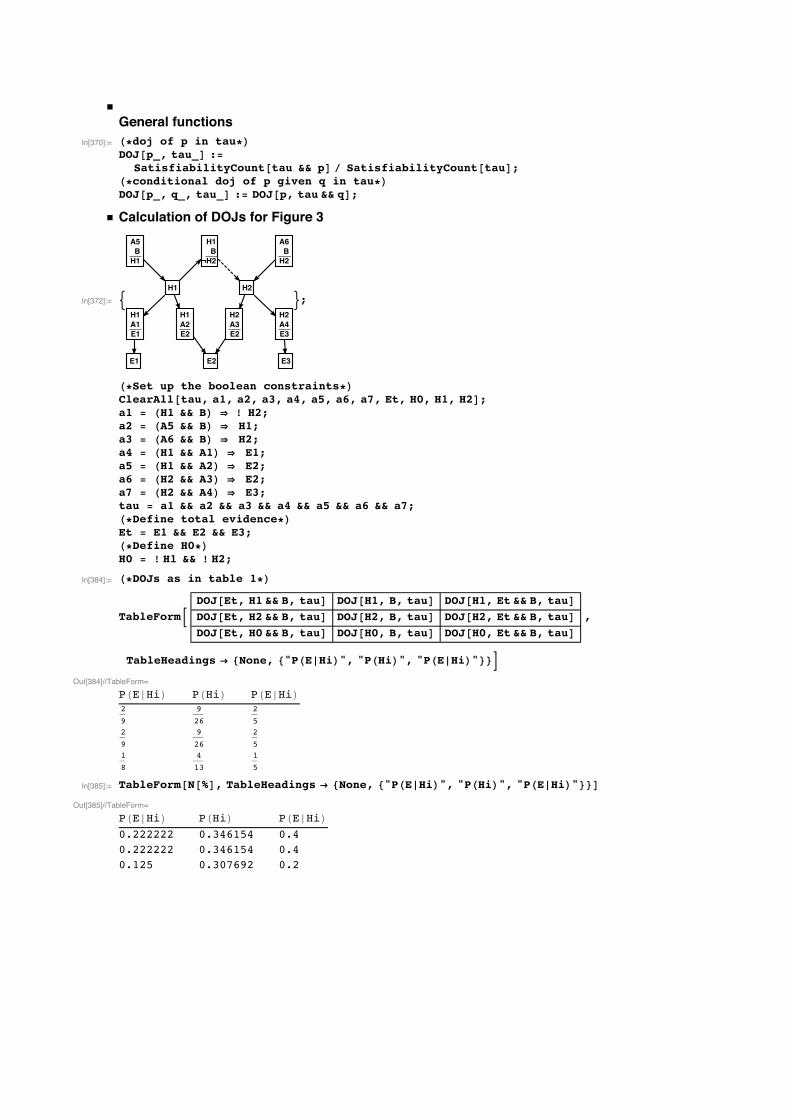
üGeneral functions
In[370]:= H*doj of p in tau*LDOJ@p_, tau_D :=
SatisfiabilityCount@tau && pD ê SatisfiabilityCount@tauD;H*conditional doj of p given q in tau*LDOJ@p_, q_, tau_D := DOJ@p, tau && qD;
ü Calculation of DOJs for Figure 3
In[372]:= : >;
H*Set up the boolean constraints*LClearAll@tau, a1, a2, a3, a4, a5, a6, a7, Et, H0, H1, H2D;a1 = HH1 && BL fl ! H2;a2 = HA5 && BL fl H1;a3 = HA6 && BL fl H2;a4 = HH1 && A1L fl E1;a5 = HH1 && A2L fl E2;a6 = HH2 && A3L fl E2;a7 = HH2 && A4L fl E3;tau = a1 && a2 && a3 && a4 && a5 && a6 && a7;H*Define total evidence*LEt = E1 && E2 && E3;H*Define H0*LH0 = ! H1 && ! H2;
In[384]:= H*DOJs as in table 1*L
TableFormBDOJ@Et, H1 && B, tauD DOJ@H1, B, tauD DOJ@H1, Et && B, tauDDOJ@Et, H2 && B, tauD DOJ@H2, B, tauD DOJ@H2, Et && B, tauDDOJ@Et, H0 && B, tauD DOJ@H0, B, tauD DOJ@H0, Et && B, tauD
,
TableHeadings Ø 8None, 8"PHE»HiL", "PHHiL", "PHE»HiL"<<F
Out[384]//TableForm=PHE»HiL PHHiL PHE»HiL2
9
9
26
2
52
9
9
26
2
51
8
4
13
1
5
In[385]:= TableForm@N@%D, TableHeadings Ø 8None, 8"PHE»HiL", "PHHiL", "PHE»HiL"<<D
Out[385]//TableForm=PHE»HiL PHHiL PHE»HiL0.222222 0.346154 0.40.222222 0.346154 0.40.125 0.307692 0.2

ü Calculation of DOJs for Figure 4
: >;
H*Set up the boolean constraints*LClearAll@tau, a1, a2, a3, a4, a5, a6, a7, Et, H0, H1, H2D;a1 = HH1 && BL fl ! H2;a2 = HA4 && BL fl H1;a3 = HA5 && BL fl H2;a4 = HH1 && BL fl E1;a5 = HH1 && BL fl E2;a6 = HH2 && A1L fl A2;a7 = HA2 && A3L fl E2;tau = a1 && a2 && a3 && a4 && a5 && a6 && a7;H*Define total evidence*LEt = E1 && E2;H*Define H0*LH0 = ! H1 && ! H2;
H*DOJs as in table 2*L
TableFormBDOJ@Et, H1 && B, tauD DOJ@H1, B, tauD DOJ@H1, Et && B, tauDDOJ@Et, H2 && B, tauD DOJ@H2, B, tauD DOJ@H2, Et && B, tauDDOJ@Et, H0 && B, tauD DOJ@H0, B, tauD DOJ@H0, Et && B, tauD
,
TableHeadings Ø 8None, 8"PHE»HiL", "PHHiL", "PHE»HiL"<<F
PHE»HiL PHHiL PHE»HiL
1 4
21
4
93
10
10
21
1
32
7
1
3
2
9
TableForm@N@%D, TableHeadings Ø 8None, 8"PHE»HiL", "PHHiL", "PHHi»EL"<<D
PHE»HiL PHHiL PHHi»EL1. 0.190476 0.4444440.3 0.47619 0.3333330.285714 0.333333 0.222222
2 dojs_ibe_examples.nb
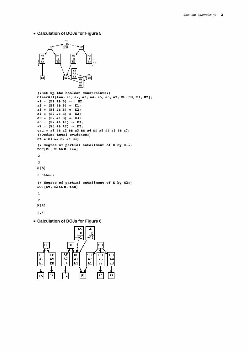
ü Calculation of DOJs for Figure 5
: >;
H*Set up the boolean constraints*LClearAll@tau, a1, a2, a3, a4, a5, a6, a7, Et, H0, H1, H2D;a1 = HH1 && BL fl ! H2;a2 = HH1 && BL fl E1;a3 = HH1 && BL fl E2;a4 = HH2 && BL fl E2;a5 = HH2 && BL fl E3;a6 = HE2 && A1L fl E3;a7 = HE3 && A2L fl E2;tau = a1 && a2 && a3 && a4 && a5 && a6 && a7;H*Define total evidence*LEt = E1 && E2 && E3;
H* degree of partial entailment of E by H1*LDOJ@Et, H1 && B, tauD
2
3N@%D
0.666667
H* degree of partial entailment of E by H2*LDOJ@Et, H2 && B, tauD
1
2N@%D
0.5
ü Calculation of DOJs for Figure 6
dojs_ibe_examples.nb 3

In[587]:= H*Set up the boolean constraints*LClearAll@tau, a1, a2, a3, a4, a5, a6, a7, a8, a9, a10, Et, H0, H1, H2, H3D;a1 = HRE && A1L fl E1;a2 = HCH && A2L fl E1;a3 = HCH && A3L fl E2;a4 = HCH && A4L fl E3;a5 = HA5 && BL fl ! A1;a6 = HA6 && BL fl ! A1;a7 = HRE && A7L fl E4;a8 = HEP && A8L fl E5;a9 = HEP && A9L fl E6;a10 = ! HEP && REL && ! HEP && CHL && ! HRE && CHL; H*hypotheses are exclusive*Ltau = a1 && a2 && a3 && a4 && a5 && a6 && a7 && a8 && a9 && a10;H*Define total evidence*LEt = E1 && E2 && E3;H*Define partial positions*LH1 = EP;H2 = RE;H3 = CH;
TableFormBDOJ@Et, H1 && B, tauD DOJ@H1, B, tauD DOJ@H1, Et && B, tauDDOJ@Et, H2 && B, tauD DOJ@H2, B, tauD DOJ@H2, Et && B, tauDDOJ@Et, H3 && B, tauD DOJ@H3, B, tauD DOJ@H3, Et && B, tauD
,
TableHeadings Ø 8None, 8"PHE»HiL", "PHHiL", "PHHi»EL"<<F
Out[602]//TableForm=PHE»HiL PHHiL PHHi»EL1
8
180
851
9
535
36
216
851
12
538
27
135
851
16
53
In[603]:= TableForm@N@%D, TableHeadings Ø 8None, 8"PHE»HiL", "PHHiL", "PHHi»EL"<<D
Out[603]//TableForm=PHE»HiL PHHiL PHHi»EL0.125 0.211516 0.1698110.138889 0.253819 0.2264150.296296 0.158637 0.301887
ü Calculation of DOJs for Figure 7
4 dojs_ibe_examples.nb

In[604]:= H*Set up the boolean constraints*LClearAll@tau, a1, a2, a3, a4, a5, a6, a7, a8, a9, a10, Et, H0, H1, H2, H3D;a1 = HSC && EML fl E1;a2 = HDI && EML fl ! E1;a3 = HDI && A2L fl E1;a4 = HCO && EML fl ! E1;a5 = HCO && A3L fl E1;a6 = HA1 && BL fl EM;a7 = ! HSC && DIL && ! HDI && COL && ! HSC && COL; H*hypotheses are exclusive*Ltau = a1 && a2 && a3 && a4 && a5 && a6 && a7;H*Define total evidence*LEt = E1 ;H*Define partial positions*LH1 = SC;H2 = DI;H3 = CO;
TableFormBDOJ@Et, H1 && B, tauD DOJ@H1, B, tauD DOJ@H1, Et && B, tauDDOJ@Et, H2 && B, tauD DOJ@H2, B, tauD DOJ@H2, Et && B, tauDDOJ@Et, H3 && B, tauD DOJ@H3, B, tauD DOJ@H3, Et && B, tauD
,
TableHeadings Ø 8None, 8"PHE»HiL", "PHHiL", "PHHi»EL"<<F
Out[616]//TableForm=PHE»HiL PHHiL PHHi»EL3
4
4
15
3
82
5
1
6
1
82
5
1
6
1
8
In[617]:= TableForm@N@%D, TableHeadings Ø 8None, 8"PHE»HiL", "PHHiL", "PHHi»EL"<<D
Out[617]//TableForm=PHE»HiL PHHiL PHHi»EL0.75 0.266667 0.3750.4 0.166667 0.1250.4 0.166667 0.125
dojs_ibe_examples.nb 5

ü Calculation of DOJs for Figure 8
: > ;
H*Set up the boolean constraints*LClearAll@tau, a1, a2, a3, a4, a5, a6, a7, Et, H0, H1, H2, H3D;a1 = HID && BL fl E1;a2 = HSW && BL fl E2;a3 = HSW && BL fl ! ID;a4 = HSW && A2L fl IO;a5 = HID && A1L fl IO;a6 = HIO && BL fl E1;a7 = HIO && BL fl E2;tau = a1 && a2 && a3 && a4 && a5 && a6 && a7;H*Define total evidence*LEt = E1 && E2;H*Define partial positions*LH1 = ID ;H2 = SW ;H3 = IO ;
H*DOJs as in table 3*L
TableFormBDOJ@Et, H1 && B, tauD DOJ@H1, B, tauD DOJ@H1, Et && B, tauDDOJ@Et, H2 && B, tauD DOJ@H2, B, tauD DOJ@H2, Et && B, tauDDOJ@Et, H3 && B, tauD DOJ@H3, B, tauD DOJ@H3, Et && B, tauD
,
TableHeadings Ø 8None, 8"PHE»HiL", "PHHiL", "PHHi»EL"<<F
PHE»HiL PHHiL PHE»HiL3
4
2
9
3
103
4
2
9
3
10
1 1
3
3
5
TableForm@N@%D, TableHeadings Ø 8None, 8"PHE»HiL", "PHHiL", "PHHi»EL"<<D
PHE»HiL PHHiL PHHi»EL0.75 0.222222 0.30.75 0.222222 0.31. 0.333333 0.6
6 dojs_ibe_examples.nb