justin g. metcalf
TRANSCRIPT

Signal Processing for Non-Gaussian Statistics: ClutterDistribution Identification and Adaptive Threshold
Estimation
By
Justin G. Metcalf
Submitted to the graduate degree program in Department of Electrical Engineering andComputer Science and the Graduate Faculty of the University of Kansas in partial
fulfillment of the requirements for the degree ofDoctor of Philosophy
Committee members
Dr. Shannon Blunt, Chairperson
Dr. Jun Huan
Dr. Tyrone Duncan
Dr. Jim Stiles
Dr. Lingjia Liu
Date defended:

The Dissertation Committee for Justin G. Metcalf certifiesthat this is the approved version of the following dissertation :
Signal Processing for Non-Gaussian Statistics: Clutter Distribution Identification andAdaptive Threshold Estimation
Dr. Shannon Blunt, Chairperson
Date approved:
ii

Abstract
We examine the problem of determining a decision threshold for the binary hy-
pothesis test that naturally arises when a radar system must decide if there is
a target present in a range cell under test. Modern radar systems require pre-
dictable, low, constant rates of false alarm (i.e. when unwanted noise and clutter
returns are mistaken for a target). Measured clutter returns have often been
fitted to heavy tailed, non-Gaussian distributions. The heavy tails on these dis-
tributions cause an unacceptable rise in the number of false alarms. We use the
class of spherically invariant random vectors (SIRVs) to model clutter returns.
SIRVs arise from a phenomenological consideration of the radar sensing prob-
lem, and include both the Gaussian distribution and most commonly reported
non-Gaussian clutter distributions (e.g. K distribution, Weibull distribution).
We propose an extension of a prior technique called the Ozturk algorithm. The
Ozturk algorithm generates a graphical library of points corresponding to known
SIRV distributions. These points are generated from linked vectors whose magni-
tude is derived from the order statistics of the SIRV distributions. Measured data
is then compared to the library and a distribution is chosen that best approx-
imates the measured data. Our extension introduces a framework of weighting
functions and examines both a distribution classification technique as well as a
method of determining an adaptive threshold in data that may or may not belong
to a known distribution. The extensions are then compared to neural networking
techniques. Special attention is paid to producing a robust, adaptive estimation
of the detection threshold. Finally, divergence measures of SIRVs are examined.

Acknowledgment
First and foremost, I would like to thank my wife, Miranda, for her loving support, encour-
agement, patience, and understanding through this journey. She provided a sea of calm
when the difficulties of graduate school were at their rockiest. I would also like to thank Dr.
Shannon Blunt for taking a chance on a Master’s student who was struggling to apply an FIR
filter. In particular, thanks for constantly encouraging me, supporting me, and imparting to
me a love and appreciation of the philosophy of our discipline. I thank Dr. Braham Himed
for his guidance, support, and for providing the genesis of this work. I would also like to
thank the Air Force Research Labs Sensors Directorate for their financial support of this
work. I would like to thank my son Mitchell, for the joy, wonder, and pride he has brought
to my life. I also thank my daughter Rosalynn, who I get to meet as I start the next step
in my journey. I would like to thank my parents, Jon and Tracy, and father-in-law Mitch
for their unwavering support and encouragement. I would also like to thank my brother
Jordan, and my sisters Brooke, Teri, and Kaylee. I hope you always embrace your dreams
and the challenges life throws at you. I would like to thank Dr. Bryce Chriestenson for the
help with the integration in Chapter 8 and the conversations on life, math, and school. I
would like to thank all of the fellow graduate students who have worked alongside me. In
particular, I would like to thank my officemates Cenk Sahin, John Jakabosky, Dr. Brian
Cordill, and Paul Anglin. Our conversations and camaraderie were intellectually stimulating
and endlessly entertaining. I would also like to thank my friend Jeff Beaver for his support
and friendship through this challenging time. Last, but certainly not least, I would like to
thank my committee, Dr. Stiles, Dr. Liu, Dr. Duncan, and Dr. Huan. Their advice and
knowledge guided me to the final product. I would also like to thank them for their patience
in wading through this dissertation.

Contents
1 Introduction 1
1.1 Radar Clutter Classification . . . . . . . . . . . . . . . . . . . . . . . . . . . 3
1.2 Mathematical Notation . . . . . . . . . . . . . . . . . . . . . . . . . . . . . . 7
2 Radar Detection 8
2.1 General Clutter Mitigation Strategies . . . . . . . . . . . . . . . . . . . . . . 10
2.2 Radar Detection in Gaussian, Homogeneous Clutter . . . . . . . . . . . . . . 14
2.3 Radar Detection in Non-Gaussian, Non-Homogenous Clutter . . . . . . . . . 18
3 Spherically Invariant Random Processes - Background 20
3.1 Real SSRVs and SIRVs . . . . . . . . . . . . . . . . . . . . . . . . . . . . . . 22
3.2 Complex SIRVs . . . . . . . . . . . . . . . . . . . . . . . . . . . . . . . . . . 27
3.3 Optimal Detection in SIRV Clutter . . . . . . . . . . . . . . . . . . . . . . . 29
3.4 Generating SIRVs . . . . . . . . . . . . . . . . . . . . . . . . . . . . . . . . . 34
3.4.1 Generating SIRV Data when the Characteristic pdf is Known . . . . 38
3.4.2 Generating SIRV Data when the Characteristic pdf is Unknown . . . 39
3.5 The K Distribution . . . . . . . . . . . . . . . . . . . . . . . . . . . . . . . . 41
3.6 The Weibull Distribution . . . . . . . . . . . . . . . . . . . . . . . . . . . . . 48
3.7 The Pareto Distribution . . . . . . . . . . . . . . . . . . . . . . . . . . . . . 50
3.8 The Lognormal Distribution . . . . . . . . . . . . . . . . . . . . . . . . . . . 51
v

4 Spherically Invariant Random Processes - New Work 54
4.1 Examining the K Distribution . . . . . . . . . . . . . . . . . . . . . . . . . . 54
4.2 Examining the Weibull Distribution . . . . . . . . . . . . . . . . . . . . . . . 61
4.3 Examining the Pareto Distribution . . . . . . . . . . . . . . . . . . . . . . . 73
4.4 Examining the Lognormal Distribution . . . . . . . . . . . . . . . . . . . . . 75
4.5 Gamma Modulated SIRV . . . . . . . . . . . . . . . . . . . . . . . . . . . . . 76
4.6 Compound Gamma Modulated SIRV . . . . . . . . . . . . . . . . . . . . . . 79
4.7 Limitations of SIRVs . . . . . . . . . . . . . . . . . . . . . . . . . . . . . . . 84
5 Distribution Estimation using Combinations of Order Statistics 86
5.1 The Ozturk Goodness-of-Fit Algorithm . . . . . . . . . . . . . . . . . . . . . 87
5.1.1 Applying the Ozturk Algorithm . . . . . . . . . . . . . . . . . . . . . 94
5.2 Weighted Sums of Ordered Statistics . . . . . . . . . . . . . . . . . . . . . . 96
5.3 Scaled Weighted Sums of Ordered Statistics . . . . . . . . . . . . . . . . . . 106
5.4 Combined Order Statistics Modeled in Clutter . . . . . . . . . . . . . . . . . 107
6 Developing the COSMiC Algorithm 127
6.1 Formal COSMiC Statement . . . . . . . . . . . . . . . . . . . . . . . . . . . 128
6.2 Initial COSMiC Evaluation . . . . . . . . . . . . . . . . . . . . . . . . . . . 135
6.3 Evaluating Pairs of Weightings in COSMiC . . . . . . . . . . . . . . . . . . . 140
6.3.1 Distribution Identification . . . . . . . . . . . . . . . . . . . . . . . . 142
6.3.2 Threshold Estimation - Identifying Top Weightings . . . . . . . . . . 148
6.3.3 Threshold Estimation - Evaluating Robustness of COSMiC Methods . 150
6.3.3.1 Gaussian Data . . . . . . . . . . . . . . . . . . . . . . . . . 151
6.3.3.2 K Data . . . . . . . . . . . . . . . . . . . . . . . . . . . . . 153
6.3.3.3 Weibull Data . . . . . . . . . . . . . . . . . . . . . . . . . . 159
6.3.3.4 Pareto Data . . . . . . . . . . . . . . . . . . . . . . . . . . . 166
6.3.3.5 Lognormal Data . . . . . . . . . . . . . . . . . . . . . . . . 173
vi

6.4 Evaluating Triplets of Weightings in COSMiC . . . . . . . . . . . . . . . . . 174
6.4.1 Distribution Identification with Triplets of Weightings . . . . . . . . . 175
6.4.2 Threshold Estimation - Identifying Top Triplet Weightings . . . . . . 178
6.4.3 Threshold Estimation with Triplets of Weightings - Evaluating Ro-
bustness of COSMiC Methods . . . . . . . . . . . . . . . . . . . . . . 180
6.4.3.1 Gaussian Data . . . . . . . . . . . . . . . . . . . . . . . . . 180
6.4.3.2 K Data . . . . . . . . . . . . . . . . . . . . . . . . . . . . . 181
6.4.3.3 Weibull Data . . . . . . . . . . . . . . . . . . . . . . . . . . 186
6.4.3.4 Pareto Data . . . . . . . . . . . . . . . . . . . . . . . . . . . 193
6.4.3.5 Lognormal Data . . . . . . . . . . . . . . . . . . . . . . . . 200
6.5 Discussion of COSMiC Results . . . . . . . . . . . . . . . . . . . . . . . . . . 201
6.5.1 Discussion of Distribution Identification . . . . . . . . . . . . . . . . 202
6.5.2 Discussion of Threshold Estimation . . . . . . . . . . . . . . . . . . . 204
6.6 Conclusions . . . . . . . . . . . . . . . . . . . . . . . . . . . . . . . . . . . . 208
7 Neural Network Approaches 210
7.1 Implementation Details . . . . . . . . . . . . . . . . . . . . . . . . . . . . . . 214
7.2 Neural Network Implementation . . . . . . . . . . . . . . . . . . . . . . . . . 218
7.2.1 Distribution Classification with Neural Networks . . . . . . . . . . . . 218
7.2.2 Threshold Estimation . . . . . . . . . . . . . . . . . . . . . . . . . . . 236
7.2.2.1 Threshold Estimation of Gaussian Data with Neural Networks237
7.2.2.2 Threshold Estimation of K Data with Neural Networks . . . 238
7.2.2.3 Threshold Estimation of Weibull Data with Neural Networks 243
7.2.2.4 Threshold Estimation of Pareto Data with Neural Networks 248
7.2.2.5 Threshold Estimation of Lognormal Data with Neural Networks253
7.2.2.6 Conclusions . . . . . . . . . . . . . . . . . . . . . . . . . . . 254
7.3 Conclusions . . . . . . . . . . . . . . . . . . . . . . . . . . . . . . . . . . . . 255
vii

8 Divergences 258
8.1 The Bregman Divergence . . . . . . . . . . . . . . . . . . . . . . . . . . . . . 258
8.2 The f Divergence . . . . . . . . . . . . . . . . . . . . . . . . . . . . . . . . . 259
8.3 The Kullback-Leibler Divergence . . . . . . . . . . . . . . . . . . . . . . . . 260
8.4 Kullback-Leibler divergence from the Gaussian distribution . . . . . . . . . . 262
8.4.1 KL divergence between the Gaussian and Pareto distributions . . . . 264
8.4.2 KL divergence between the Gaussian and K distributions . . . . . . . 274
8.5 Conclusions . . . . . . . . . . . . . . . . . . . . . . . . . . . . . . . . . . . . 281
9 Conclusions and Future Work 282
9.1 Summary . . . . . . . . . . . . . . . . . . . . . . . . . . . . . . . . . . . . . 282
9.2 Future Work . . . . . . . . . . . . . . . . . . . . . . . . . . . . . . . . . . . . 291
9.3 Conclusions . . . . . . . . . . . . . . . . . . . . . . . . . . . . . . . . . . . . 296
A COSMiC Weighting Comparison Tables 319
A.1 Pairwise Distribution Identification . . . . . . . . . . . . . . . . . . . . . . . 319
A.1.1 Gaussian Distributed Data . . . . . . . . . . . . . . . . . . . . . . . . 319
A.1.2 K Distributed Data . . . . . . . . . . . . . . . . . . . . . . . . . . . . 321
A.1.3 Weibull Distributed Data . . . . . . . . . . . . . . . . . . . . . . . . 322
A.1.4 Pareto Distributed Data . . . . . . . . . . . . . . . . . . . . . . . . . 324
A.1.5 Lognormal Distributed Data . . . . . . . . . . . . . . . . . . . . . . . 325
A.2 Pairwise Threshold Estimation . . . . . . . . . . . . . . . . . . . . . . . . . . 327
A.3 Tables for Distribution Identification using Triplets of Weightings . . . . . . 329
A.3.1 Gaussian Distributed Data . . . . . . . . . . . . . . . . . . . . . . . . 329
A.3.2 K Distributed Data . . . . . . . . . . . . . . . . . . . . . . . . . . . . 331
A.3.3 Weibull Distributed Data . . . . . . . . . . . . . . . . . . . . . . . . 332
A.3.4 Pareto Distributed Data . . . . . . . . . . . . . . . . . . . . . . . . . 334
A.3.5 Lognormal Distributed Data . . . . . . . . . . . . . . . . . . . . . . . 335
viii

A.4 Tables for Threshold Estimation using Triplets of Weightings . . . . . . . . . 337
B Deep Belief Network Strategies 345
B.1 Two Stage Threshold Estimating Deep Network . . . . . . . . . . . . . . . . 346
B.1.1 Threshold Estimation of Gaussian Data with a Deep Neural Network 348
B.1.2 Threshold Estimation of K Data with a Deep Neural Network . . . . 348
B.1.3 Threshold Estimation of Weibull Data with a Deep Neural Network . 353
B.1.4 Threshold Estimation of Pareto Data with a Deep Neural Network . . 358
B.1.5 Threshold Estimation of Lognormal Data with a Deep Neural Network 363
B.2 Three Stage Threshold Estimating Deep Network . . . . . . . . . . . . . . . 364
B.2.1 Threshold Estimation of Gaussian Data with a Deep Neural Network 366
B.2.2 Threshold Estimation of K Data with a Deep Neural Network . . . . 367
B.2.3 Threshold Estimation of Weibull Data with a Deep Neural Network . 372
B.2.4 Threshold Estimation of Pareto Data with a Deep Neural Network . . 377
B.2.5 Threshold Estimation of Lognormal Data with a Deep Neural Network 382
C Current Literature Applying Covariance Matrix Estimation to SIRV Data384
C.1 Non-Homogeneity Detection . . . . . . . . . . . . . . . . . . . . . . . . . . . 384
C.2 Investigating the Impact of Measured Sea Clutter Non-Stationarity . . . . . 387
ix

List of Figures
2.1 An example of an airborne radar . . . . . . . . . . . . . . . . . . . . . . . . 11
2.2 An example CFAR detector . . . . . . . . . . . . . . . . . . . . . . . . . . . 16
3.1 Rejection Method Example . . . . . . . . . . . . . . . . . . . . . . . . . . . 36
3.2 Rejection Method Example . . . . . . . . . . . . . . . . . . . . . . . . . . . 37
3.3 Generation of Arbitrary SIRV Data with Known Characteristic pdf . . . . . 39
3.4 cdfs of the K distribution for increasing shape parameter . . . . . . . . . . . 42
4.1 pdf of fV (v) for increasing shape parameter . . . . . . . . . . . . . . . . . . 55
4.2 Analytic and simulated pdf for K distribution for low values of ν . . . . . . 57
4.3 Comparing K distribution pdfs and cdfs for small values of ν . . . . . . . . . 57
4.4 Impact of K distribution for small values of ν on NP test . . . . . . . . . . . 58
4.5 Analytic and simulated pdf for K distribution for medium values of ν . . . . 59
4.6 Comparing pdfs and cdfs of the K distribution for medium values of ν . . . . 59
4.7 Impact of K distribution for medium values of ν on NP test . . . . . . . . . 60
4.8 Comparing pdfs and cdfs of the K distribution for large values of ν . . . . . 60
4.9 Impact of K distribution for large values of ν on NP test . . . . . . . . . . . 61
4.10 Examples of numerical integration of the cdf of the Weibull SIRV . . . . . . 66
4.11 Finding approximate values of c and k with the estimated CDF of a Weibull
distribution for ν = 0.3 . . . . . . . . . . . . . . . . . . . . . . . . . . . . . . 67
x

4.12 Finding approximate values of c and k with the estimated CDF of a Weibull
distribution for ν = 0.7 . . . . . . . . . . . . . . . . . . . . . . . . . . . . . . 68
4.13 Finding approximate values of c and k with the estimated CDF of a Weibull
distribution for ν = 0.8 . . . . . . . . . . . . . . . . . . . . . . . . . . . . . . 68
4.14 Finding approximate values of c and k with the estimated CDF of a Weibull
distribution for ν = 1.01 . . . . . . . . . . . . . . . . . . . . . . . . . . . . . 69
4.15 Comparing analytic and simulated distributions of the Weibull envelope for
ν = 0.9 . . . . . . . . . . . . . . . . . . . . . . . . . . . . . . . . . . . . . . . 70
4.16 Comparing analytic and simulated distributions of the Weibull envelope for
ν = 1.1 . . . . . . . . . . . . . . . . . . . . . . . . . . . . . . . . . . . . . . . 71
4.17 Comparing analytic and simulated distributions of a complex Weibull SIRV
for ν = 1 . . . . . . . . . . . . . . . . . . . . . . . . . . . . . . . . . . . . . . 72
4.18 ∆thresh in log scale for the Weibull distribution for increasing shape parameter 73
4.19 pdf and cdf of quadratic form of Pareto clutter . . . . . . . . . . . . . . . . . 74
4.20 Consequences of Pareto clutter . . . . . . . . . . . . . . . . . . . . . . . . . 74
4.21 Empirical pdf and cdf of the GIP of complex lognormal data for length L = 4
vectors . . . . . . . . . . . . . . . . . . . . . . . . . . . . . . . . . . . . . . 75
4.22 cdfs of the GM SIRV distribution . . . . . . . . . . . . . . . . . . . . . . . . 78
4.23 Threshold and Pfa properties of the GM SIRV . . . . . . . . . . . . . . . . . 79
4.24 cdfs of the CGM SIRV distribution . . . . . . . . . . . . . . . . . . . . . . . 82
4.25 ∆thresh (dB) for the CGM SIRV as a function of shape parameter . . . . . . 83
4.26 Pfa for the CGM SIRV as a function of shape parameter . . . . . . . . . . . 84
5.1 Illustration of linked vectors (reprinted from [1]) . . . . . . . . . . . . . . . . 91
5.2 Library of endpoints for SIRV identification (reprinted from [1]) . . . . . . . 92
5.3 Implementation of the Ozturk algorithm . . . . . . . . . . . . . . . . . . . . 93
5.5 Implementation of Ozturk algorithm on MCARM data file rd050465 . . . . . 96
5.6 Comparing sine and cosine derived weightings . . . . . . . . . . . . . . . . . 99
xi

5.7 Comparing sinh, cosh, and tanh derived weightings . . . . . . . . . . . . . . 100
5.8 pdf and cdf of example K distributed SIRV . . . . . . . . . . . . . . . . . . . 101
5.9 Endpoint distribution for sin and sin2 . . . . . . . . . . . . . . . . . . . . . . 102
5.10 Endpoint distribution for cos and cos2 . . . . . . . . . . . . . . . . . . . . . 102
5.11 Endpoint distribution for cosh, cosh2, tanh, and tanh2 . . . . . . . . . . . . . 103
5.12 Endpoint distribution for sinh and sinh2 . . . . . . . . . . . . . . . . . . . . 104
5.13 Endpoint distributions for pairs of weighting functions with K distributed data105
5.14 COSMiC Flowcharts . . . . . . . . . . . . . . . . . . . . . . . . . . . . . . . 109
5.15 Example non-linear transform: weighted sum of order statistics . . . . . . . . 109
5.16 COSMiC endpoint distributions, cosine v. sine . . . . . . . . . . . . . . . . . 112
5.17 COSMiC endpoint distributions for cosine v. threshold . . . . . . . . . . . . 113
5.18 Ambiguity for cosine v. threshold . . . . . . . . . . . . . . . . . . . . . . . . 114
5.19 COSMiC endpoint distributions for sine v. threshold . . . . . . . . . . . . . 116
5.20 COSMiC endpoint distributions, sine squared v. cosine squared . . . . . . . 117
5.21 COSMiC endpoint distributions for cosine squared v. threshold . . . . . . . 118
5.22 COSMiC endpoint distributions for sine squared v. threshold . . . . . . . . . 120
5.23 COSMiC endpoint distributions, cosh v. sinh . . . . . . . . . . . . . . . . . . 121
5.24 COSMiC endpoint distributions for cosh v. threshold . . . . . . . . . . . . . 122
5.25 COSMiC endpoint distributions for sinh v. threshold . . . . . . . . . . . . . 123
5.26 COSMiC endpoint distributions, tanh v. sine . . . . . . . . . . . . . . . . . . 124
5.27 COSMiC endpoint distributions for tanh v. threshold . . . . . . . . . . . . . 125
6.1 Data pre-processing block diagram . . . . . . . . . . . . . . . . . . . . . . . 129
6.2 COSMiC distribution identification block diagram . . . . . . . . . . . . . . . 132
6.3 COSMiC threshold estimation block diagram . . . . . . . . . . . . . . . . . . 134
6.4 Using the EOA to classify K data as a function of shape (reprinted from [2]) 136
6.5 Using the EOA to estimate threshold as a function of shape (reprinted from [2])137
xii

6.6 Using the EOA to classify K data as a function of shape with lognormal
distribution omitted from library . . . . . . . . . . . . . . . . . . . . . . . . 140
6.7 COSMiC distribution identification v. shape parameter for K distributed data
for top pairs . . . . . . . . . . . . . . . . . . . . . . . . . . . . . . . . . . . . 145
6.8 COSMiC distribution identification v. shape parameter for Weibull distributed
data for top pairs . . . . . . . . . . . . . . . . . . . . . . . . . . . . . . . . . 146
6.9 COSMiC distribution identification v. shape parameter for Pareto distributed
data for top pairs . . . . . . . . . . . . . . . . . . . . . . . . . . . . . . . . . 147
6.10 Threshold estimation error (dB) using WSOS with K distributed data . . . . 154
6.11 Threshold estimation error (dB) using DBM with K distributed data . . . . 155
6.12 Threshold estimation error (dB) using Studentized method with K distributed
data . . . . . . . . . . . . . . . . . . . . . . . . . . . . . . . . . . . . . . . . 157
6.13 Threshold estimation error (dB) using EOA method with K distributed data 159
6.14 Threshold estimation error (dB) using WSOS with Weibull distributed data 161
6.15 Threshold estimation error (dB) using DBM with Weibull distributed data . 162
6.16 Threshold estimation error (dB) using Studentized method with Weibull dis-
tributed data . . . . . . . . . . . . . . . . . . . . . . . . . . . . . . . . . . . 163
6.17 Threshold estimation error (dB) using EOA method with Weibull distributed
data . . . . . . . . . . . . . . . . . . . . . . . . . . . . . . . . . . . . . . . . 165
6.18 Threshold estimation error (dB) using WSOS with Pareto distributed data . 167
6.19 Threshold estimation error (dB) using DBM with Pareto distributed data . . 168
6.20 Threshold estimation error (dB) using Studentized method with Pareto dis-
tributed data . . . . . . . . . . . . . . . . . . . . . . . . . . . . . . . . . . . 170
6.21 Threshold estimation error (dB) using EOA method with Pareto distributed
data . . . . . . . . . . . . . . . . . . . . . . . . . . . . . . . . . . . . . . . . 172
6.22 COSMiC distribution identification vs. shape parameter for Weibull dis-
tributed data for top triplets . . . . . . . . . . . . . . . . . . . . . . . . . . . 176
xiii

6.23 COSMiC distribution identification vs. shape parameter for Weibull dis-
tributed data for top triplets . . . . . . . . . . . . . . . . . . . . . . . . . . . 177
6.24 COSMiC distribution identification v. shape parameter for Pareto distributed
data for top triplets . . . . . . . . . . . . . . . . . . . . . . . . . . . . . . . . 178
6.25 Threshold estimation error (dB) using WSOS with K distributed data . . . . 182
6.26 Threshold estimation error (dB) using DBM with K distributed data . . . . 183
6.27 Threshold estimation error (dB) using Studentized method with K distributed
data . . . . . . . . . . . . . . . . . . . . . . . . . . . . . . . . . . . . . . . . 184
6.28 Threshold estimation error (dB) using EOA method with K distributed data 185
6.29 Threshold estimation error (dB) using WSOS with Weibull distributed data 187
6.30 Threshold estimation error (dB) using DBM with Weibull distributed data . 188
6.31 Threshold estimation error (dB) using Studentized method with Weibull dis-
tributed data . . . . . . . . . . . . . . . . . . . . . . . . . . . . . . . . . . . 190
6.32 Threshold estimation error (dB) using EOA method with Weibull distributed
data . . . . . . . . . . . . . . . . . . . . . . . . . . . . . . . . . . . . . . . . 192
6.33 Threshold estimation error (dB) using WSOS with Pareto distributed data . 194
6.34 Threshold estimation error (dB) using DBM with Pareto distributed data . . 195
6.35 Threshold estimation error (dB) using Studentized method with Pareto dis-
tributed data . . . . . . . . . . . . . . . . . . . . . . . . . . . . . . . . . . . 197
6.36 Threshold estimation error (dB) using EOA method with Pareto distributed
data . . . . . . . . . . . . . . . . . . . . . . . . . . . . . . . . . . . . . . . . 199
7.1 Simple and expanded perceptron models . . . . . . . . . . . . . . . . . . . . 211
7.2 Example multilayer perceptron neural network . . . . . . . . . . . . . . . . . 212
7.3 Distribution identification neural network . . . . . . . . . . . . . . . . . . . . 219
7.4 Distribution identification by neural networks for unordered K distributed data223
7.5 Distribution identification by neural networks for ordered K distributed data 225
xiv

7.6 Distribution identification by neural networks for unorderedWeibull distributed
data . . . . . . . . . . . . . . . . . . . . . . . . . . . . . . . . . . . . . . . . 227
7.7 Distribution identification by neural networks for ordered Weibull distributed
data . . . . . . . . . . . . . . . . . . . . . . . . . . . . . . . . . . . . . . . . 229
7.8 Distribution identification by neural networks for unordered Pareto distributed
data . . . . . . . . . . . . . . . . . . . . . . . . . . . . . . . . . . . . . . . . 231
7.9 Distribution identification by neural networks for ordered Pareto distributed
data . . . . . . . . . . . . . . . . . . . . . . . . . . . . . . . . . . . . . . . . 233
7.10 Threshold estimation neural network . . . . . . . . . . . . . . . . . . . . . . 236
7.11 Threshold estimation by neural networks for unordered K distributed data . 240
7.12 Threshold estimation by neural networks for ordered K distributed data . . . 241
7.13 Threshold estimation by neural networks for unordered K distributed data, K
data not included in training data . . . . . . . . . . . . . . . . . . . . . . . . 242
7.14 Threshold estimation by neural networks for ordered K distributed data, K
data not included in training data . . . . . . . . . . . . . . . . . . . . . . . . 243
7.15 Threshold estimation by neural networks for unordered Weibull distributed
data . . . . . . . . . . . . . . . . . . . . . . . . . . . . . . . . . . . . . . . . 245
7.16 Threshold estimation by neural networks for ordered Weibull distributed data 246
7.17 Threshold estimation by neural networks for unordered Weibull distributed
data, Weibull data not included in training data . . . . . . . . . . . . . . . . 247
7.18 Threshold estimation by neural networks for ordered Weibull distributed data,
Weibull data not included in training data . . . . . . . . . . . . . . . . . . . 248
7.19 Threshold estimation by neural networks for unordered Pareto distributed data250
7.20 Threshold estimation by neural networks for ordered Pareto distributed data 251
7.21 Threshold estimation by neural networks for unordered Pareto distributed
data, Pareto data not included in training data . . . . . . . . . . . . . . . . 252
xv

7.22 Threshold estimation by neural networks for ordered Pareto distributed data,
Pareto data not included in training data . . . . . . . . . . . . . . . . . . . . 253
8.1 Kullback-Leibler divergence (in dB) between Gaussian and Pareto distribu-
tions for vector length L = 4 . . . . . . . . . . . . . . . . . . . . . . . . . . . 274
B.1 Deep neural network for threshold estimation . . . . . . . . . . . . . . . . . 347
B.2 Threshold estimation by a deep neural network for unordered K distributed
data . . . . . . . . . . . . . . . . . . . . . . . . . . . . . . . . . . . . . . . . 350
B.3 Threshold estimation by a deep neural network for ordered K distributed data 351
B.4 Threshold estimation by a deep neural network for unordered K distributed
data, K data not included in training data . . . . . . . . . . . . . . . . . . . 352
B.5 Threshold estimation by a deep neural network for ordered K distributed data,
K data not included in training data . . . . . . . . . . . . . . . . . . . . . . 353
B.6 Threshold estimation by a deep neural network for unordered Weibull dis-
tributed data . . . . . . . . . . . . . . . . . . . . . . . . . . . . . . . . . . . 355
B.7 Threshold estimation by a deep neural network for ordered Weibull distributed
data . . . . . . . . . . . . . . . . . . . . . . . . . . . . . . . . . . . . . . . . 356
B.8 Threshold estimation by a deep neural network for unordered Weibull dis-
tributed data, Weibull data not included in training data . . . . . . . . . . . 357
B.9 Threshold estimation by a deep neural network for ordered Weibull distributed
data, Weibull data not included in training data . . . . . . . . . . . . . . . . 358
B.10 Threshold estimation by a deep neural network for unordered Pareto dis-
tributed data . . . . . . . . . . . . . . . . . . . . . . . . . . . . . . . . . . . 360
B.11 Threshold estimation by a deep neural network for ordered Pareto distributed
data . . . . . . . . . . . . . . . . . . . . . . . . . . . . . . . . . . . . . . . . 361
B.12 Threshold estimation by a deep neural network for unordered Pareto dis-
tributed data, Pareto data not included in training data . . . . . . . . . . . 362
xvi

B.13 Threshold estimation by a deep neural network for ordered Pareto distributed
data, Pareto data not included in training data . . . . . . . . . . . . . . . . 363
B.14 Deep neural network for threshold estimation . . . . . . . . . . . . . . . . . 365
B.15 Deep neural network - shape parameter estimating neural networks . . . . . 365
B.16 Deep neural network for threshold estimation - threshold estimating neural
networks with augmented input . . . . . . . . . . . . . . . . . . . . . . . . . 366
B.17 Threshold estimation by a three stage deep neural network for unordered K
distributed data . . . . . . . . . . . . . . . . . . . . . . . . . . . . . . . . . . 369
B.18 Threshold estimation by a three stage deep neural network for ordered K
distributed data . . . . . . . . . . . . . . . . . . . . . . . . . . . . . . . . . . 370
B.19 Threshold estimation by a three stage deep neural network for unordered K
distributed data, K data not included in training data . . . . . . . . . . . . . 371
B.20 Threshold estimation by a three stage deep neural network for ordered K
distributed data, K data not included in training data . . . . . . . . . . . . . 372
B.21 Threshold estimation by a three stage deep neural network for unordered
Weibull distributed data . . . . . . . . . . . . . . . . . . . . . . . . . . . . . 374
B.22 Threshold estimation by a three stage deep neural network for ordered Weibull
distributed data . . . . . . . . . . . . . . . . . . . . . . . . . . . . . . . . . . 375
B.23 Threshold estimation by a three stage deep neural network for unordered
Weibull distributed data, Weibull data not included in training data . . . . . 376
B.24 Threshold estimation by a three stage deep neural network for ordered Weibull
distributed data, Weibull data not included in training data . . . . . . . . . 377
B.25 Threshold estimation by a three stage deep neural network for unordered
Pareto distributed data . . . . . . . . . . . . . . . . . . . . . . . . . . . . . . 379
B.26 Threshold estimation by a three stage deep neural network for ordered Pareto
distributed data . . . . . . . . . . . . . . . . . . . . . . . . . . . . . . . . . . 380
xvii

B.27 Threshold estimation by a three stage deep neural network for unordered
Pareto distributed data, Pareto data not included in training data . . . . . . 381
B.28 Threshold estimation by a three stage deep neural network for ordered Pareto
distributed data, Pareto data not included in training data . . . . . . . . . . 382
xviii

List of Tables
1 List of Acronyms . . . . . . . . . . . . . . . . . . . . . . . . . . . . . . . . . xxviii
6.1 Distribution identification percentages of top WSOS COSMiC weighting pairs 142
6.2 Distribution identification percentages of top Studentized COSMiC weighting
pairs . . . . . . . . . . . . . . . . . . . . . . . . . . . . . . . . . . . . . . . . 143
6.3 Distribution identification percentages of top EOA COSMiC weighting pairs 143
6.4 Summary of top WSOS COSMiC weighting pairs . . . . . . . . . . . . . . . 149
6.5 Summary of top Studentized COSMiC weighting pairs . . . . . . . . . . . . 150
6.6 Summary of top Extended Ozturk COSMiC weighting pairs . . . . . . . . . 150
6.7 Average Threshold Error (dB) when Gaussian distributed data is fed into the
WSOS and DBM weightings . . . . . . . . . . . . . . . . . . . . . . . . . . . 152
6.8 Average Threshold Error (dB) when Gaussian distributed data is fed into the
Studentized weightings . . . . . . . . . . . . . . . . . . . . . . . . . . . . . . 152
6.9 Average Threshold Error (dB) when Gaussian distributed data is fed into the
EOA weightings . . . . . . . . . . . . . . . . . . . . . . . . . . . . . . . . . . 152
6.10 Average Threshold Error (dB) when K distributed data is fed into the WSOS
and DBM weightings . . . . . . . . . . . . . . . . . . . . . . . . . . . . . . . 153
6.11 Average Threshold Error (dB) when K distributed data is fed into the Stu-
dentized weightings . . . . . . . . . . . . . . . . . . . . . . . . . . . . . . . . 156
6.12 Average Threshold Error (dB) when K distributed data is fed into the EOA
weightings . . . . . . . . . . . . . . . . . . . . . . . . . . . . . . . . . . . . . 158
xix

6.13 Average Threshold Error (dB) when Weibull distributed data is fed into the
WSOS and DBM weightings . . . . . . . . . . . . . . . . . . . . . . . . . . . 160
6.14 Average Threshold Error (dB) when Weibull distributed data is fed into the
Studentized weightings . . . . . . . . . . . . . . . . . . . . . . . . . . . . . . 162
6.15 Average Threshold Error (dB) when Weibull distributed data is fed into the
EOA weightings . . . . . . . . . . . . . . . . . . . . . . . . . . . . . . . . . . 164
6.16 Average Threshold Error (dB) when Pareto distributed data is fed into the
WSOS and DBM weightings . . . . . . . . . . . . . . . . . . . . . . . . . . . 166
6.17 Average Threshold Error (dB) when Pareto distributed data is fed into the
Studentized weightings . . . . . . . . . . . . . . . . . . . . . . . . . . . . . . 169
6.18 Average Threshold Error (dB) when Pareto distributed data is fed into the
EOA weightings . . . . . . . . . . . . . . . . . . . . . . . . . . . . . . . . . . 171
6.19 Average Threshold Error (dB) when Lognormal distributed data is fed into
the WSOS and DBM weightings . . . . . . . . . . . . . . . . . . . . . . . . . 173
6.20 Average Threshold Error (dB) when Lognormal distributed data is fed into
the Studentized weightings . . . . . . . . . . . . . . . . . . . . . . . . . . . . 173
6.21 Average Threshold Error (dB) when Lognormal distributed data is fed into
the EOA weightings . . . . . . . . . . . . . . . . . . . . . . . . . . . . . . . . 174
6.22 Distribution identification percentages of top WSOS COSMiC weighting triplets175
6.23 Distribution identification percentages of top Studentized COSMiC weighting
triplets . . . . . . . . . . . . . . . . . . . . . . . . . . . . . . . . . . . . . . . 175
6.24 Distribution identification percentages of top EOA COSMiC weighting triplets 175
6.25 Summary of top WSOS weighting triplets . . . . . . . . . . . . . . . . . . . 179
6.26 Summary of top studentized weighting triplets . . . . . . . . . . . . . . . . . 179
6.27 Summary of top extended Ozturk weighting triplets . . . . . . . . . . . . . . 179
6.28 Average Threshold Error (dB) when Gaussian distributed data is fed into the
WSOS and DBM weightings . . . . . . . . . . . . . . . . . . . . . . . . . . . 180
xx

6.29 Average Threshold Error (dB) when Gaussian distributed data is fed into the
Studentized weightings . . . . . . . . . . . . . . . . . . . . . . . . . . . . . . 180
6.30 Average Threshold Error (dB) when Gaussian distributed data is fed into the
EOA weightings . . . . . . . . . . . . . . . . . . . . . . . . . . . . . . . . . . 181
6.31 Average Threshold Error (dB) when K distributed data is fed into the WSOS
and DBM weightings . . . . . . . . . . . . . . . . . . . . . . . . . . . . . . . 181
6.32 Average Threshold Error (dB) when K distributed data is fed into the Stu-
dentized weightings . . . . . . . . . . . . . . . . . . . . . . . . . . . . . . . . 184
6.33 Average Threshold Error (dB) when K distributed data is fed into the EOA
weightings . . . . . . . . . . . . . . . . . . . . . . . . . . . . . . . . . . . . . 185
6.34 Average Threshold Error (dB) when Weibull distributed data is fed into the
WSOS and DBM weightings . . . . . . . . . . . . . . . . . . . . . . . . . . . 186
6.35 Average Threshold Error (dB) when Weibull distributed data is fed into the
Studentized weightings . . . . . . . . . . . . . . . . . . . . . . . . . . . . . . 189
6.36 Average Threshold Error (dB) when Weibull distributed data is fed into the
EOA weightings . . . . . . . . . . . . . . . . . . . . . . . . . . . . . . . . . . 191
6.37 Average Threshold Error (dB) when Pareto distributed data is fed into the
WSOS and DBM weightings . . . . . . . . . . . . . . . . . . . . . . . . . . . 193
6.38 Average Threshold Error (dB) when Pareto distributed data is fed into the
Studentized weightings . . . . . . . . . . . . . . . . . . . . . . . . . . . . . . 196
6.39 Average Threshold Error (dB) when Pareto distributed data is fed into the
EOA weightings . . . . . . . . . . . . . . . . . . . . . . . . . . . . . . . . . . 198
6.40 Average Threshold Error (dB) when Lognormal distributed data is fed into
the WSOS and DBM weightings . . . . . . . . . . . . . . . . . . . . . . . . . 200
6.41 Average Threshold Error (dB) when Lognormal distributed data is fed into
the Studentized weightings . . . . . . . . . . . . . . . . . . . . . . . . . . . . 200
xxi

6.42 Average Threshold Error (dB) when Lognormal distributed data is fed into
the EOA weightings . . . . . . . . . . . . . . . . . . . . . . . . . . . . . . . . 201
6.43 Summary of the best COSMiC transformation methods and weightings . . . 206
7.1 Number of shape parameter values by distribution used to train neural networks217
7.2 Neural network training parameters summary . . . . . . . . . . . . . . . . . 218
7.3 Distribution identification percentages of Neural Networks for unordered Gaus-
sian Distributed data . . . . . . . . . . . . . . . . . . . . . . . . . . . . . . . 221
7.4 Distribution identification percentages of Neural Networks for ordered Gaus-
sian Distributed data . . . . . . . . . . . . . . . . . . . . . . . . . . . . . . . 221
7.5 Distribution identification percentages of Neural Networks for unordered K
Distributed data . . . . . . . . . . . . . . . . . . . . . . . . . . . . . . . . . 222
7.6 Distribution identification percentages of Neural Networks for ordered K Dis-
tributed data . . . . . . . . . . . . . . . . . . . . . . . . . . . . . . . . . . . 224
7.7 Distribution identification percentages of Neural Networks for unorderedWeibull
Distributed data . . . . . . . . . . . . . . . . . . . . . . . . . . . . . . . . . 226
7.8 Distribution identification percentages of Neural Networks for ordered Weibull
Distributed data . . . . . . . . . . . . . . . . . . . . . . . . . . . . . . . . . 228
7.9 Distribution identification percentages of Neural Networks for unordered Pareto
Distributed data . . . . . . . . . . . . . . . . . . . . . . . . . . . . . . . . . 230
7.10 Distribution identification percentages of Neural Networks for ordered Pareto
Distributed data . . . . . . . . . . . . . . . . . . . . . . . . . . . . . . . . . 232
7.11 Distribution identification percentages of Neural Networks for unordered Log-
normal Distributed data . . . . . . . . . . . . . . . . . . . . . . . . . . . . . 234
7.12 Distribution identification percentages of Neural Networks for ordered Log-
normal Distributed data . . . . . . . . . . . . . . . . . . . . . . . . . . . . . 234
7.13 Average Threshold Error (dB) when Gaussian data is fed into single layer
neural networks . . . . . . . . . . . . . . . . . . . . . . . . . . . . . . . . . . 238
xxii
7.14 Average Threshold Error (dB) when K data is fed into single layer neural
networks . . . . . . . . . . . . . . . . . . . . . . . . . . . . . . . . . . . . . . 239
7.15 Average Threshold Error (dB) when Weibull data is fed into single layer neural
networks . . . . . . . . . . . . . . . . . . . . . . . . . . . . . . . . . . . . . . 244
7.16 Average Threshold Error (dB) when Pareto data is fed into single layer neural
networks . . . . . . . . . . . . . . . . . . . . . . . . . . . . . . . . . . . . . . 249
7.17 Average Threshold Error (dB) when lognormal data is fed into single layer
neural networks . . . . . . . . . . . . . . . . . . . . . . . . . . . . . . . . . . 254
A.1 Distribution identification percentages of top 10 WSOS COSMiC weighting
pairs for Gaussian Distributed data . . . . . . . . . . . . . . . . . . . . . . . 319
A.2 Distribution identification percentages of top 10 Studentized COSMiC weight-
ing pairs for Gaussian Distributed data . . . . . . . . . . . . . . . . . . . . . 320
A.3 Distribution identification percentages of top 10 EOA COSMiC weighting
pairs for Gaussian Distributed data . . . . . . . . . . . . . . . . . . . . . . . 320
A.4 Distribution identification percentages of top 10 WSOS COSMiC weighting
pairs for K Distributed data . . . . . . . . . . . . . . . . . . . . . . . . . . . 321
A.5 Distribution identification percentages of top 10 Studentized COSMiC weight-
ing pairs for K Distributed data . . . . . . . . . . . . . . . . . . . . . . . . . 321
A.6 Distribution identification percentages of top 10 EOA COSMiC weighting
pairs for K Distributed data . . . . . . . . . . . . . . . . . . . . . . . . . . . 322
A.7 Distribution identification percentages of top 10 WSOS COSMiC weighting
pairs for Weibull Distributed data . . . . . . . . . . . . . . . . . . . . . . . . 322
A.8 Distribution identification percentages of top 10 Studentized COSMiC weight-
ing pairs for Weibull Distributed data . . . . . . . . . . . . . . . . . . . . . . 323
A.9 Distribution identification percentages of top 10 EOA COSMiC weighting
pairs for Weibull Distributed data . . . . . . . . . . . . . . . . . . . . . . . . 323
xxiii

A.10 Distribution identification percentages of top 10 WSOS COSMiC weighting
pairs for Pareto Distributed data . . . . . . . . . . . . . . . . . . . . . . . . 324
A.11 Distribution identification percentages of top 10 Studentized COSMiC weight-
ing pairs for Pareto Distributed data . . . . . . . . . . . . . . . . . . . . . . 324
A.12 Distribution identification percentages of top 10 EOA COSMiC weighting
pairs for Pareto Distributed data . . . . . . . . . . . . . . . . . . . . . . . . 325
A.13 Distribution identification percentages of top 10 WSOS COSMiC weighting
pairs for lognormal Distributed data . . . . . . . . . . . . . . . . . . . . . . 325
A.14 Distribution identification percentages of top 10 Studentized COSMiC weight-
ing pairs for lognormal Distributed data . . . . . . . . . . . . . . . . . . . . 326
A.15 Distribution identification percentages of top 10 EOA COSMiC weighting
pairs for lognormal Distributed data . . . . . . . . . . . . . . . . . . . . . . 326
A.16 Average threshold estimation error in dB for COSMiC with Gaussian dis-
tributed data . . . . . . . . . . . . . . . . . . . . . . . . . . . . . . . . . . . 327
A.17 Average threshold estimation error in dB for COSMiC with K distributed data 327
A.18 Average threshold estimation error in dB for COSMiC with Weibull dis-
tributed data . . . . . . . . . . . . . . . . . . . . . . . . . . . . . . . . . . . 328
A.19 Average threshold estimation error in dB for COSMiC with Pareto distributed
data . . . . . . . . . . . . . . . . . . . . . . . . . . . . . . . . . . . . . . . . 328
A.20 Average threshold estimation error in dB for COSMiC with lognormal dis-
tributed data . . . . . . . . . . . . . . . . . . . . . . . . . . . . . . . . . . . 329
A.21 Distribution identification percentages of top 10 WSOS COSMiC weighting
triplets for Gaussian Distributed data . . . . . . . . . . . . . . . . . . . . . . 329
A.22 Distribution identification percentages of top 10 Studentized COSMiC weight-
ing triplets for Gaussian Distributed data . . . . . . . . . . . . . . . . . . . . 330
A.23 Distribution identification percentages of top 10 EOA COSMiC weighting
triplets for Gaussian Distributed data . . . . . . . . . . . . . . . . . . . . . . 330
xxiv

A.24 Distribution identification percentages of top 10 WSOS COSMiC weighting
triplets for K Distributed data . . . . . . . . . . . . . . . . . . . . . . . . . . 331
A.25 Distribution identification percentages of top 10 Studentized COSMiC weight-
ing triplets for K Distributed data . . . . . . . . . . . . . . . . . . . . . . . . 331
A.26 Distribution identification percentages of top 10 EOA COSMiC weighting
triplets for K Distributed data . . . . . . . . . . . . . . . . . . . . . . . . . . 332
A.27 Distribution identification percentages of top 10 WSOS COSMiC weighting
triplets for Weibull Distributed data . . . . . . . . . . . . . . . . . . . . . . 332
A.28 Distribution identification percentages of top 10 Studentized COSMiC weight-
ing triplets for Weibull Distributed data . . . . . . . . . . . . . . . . . . . . 333
A.29 Distribution identification percentages of top 10 EOA COSMiC weighting
triplets for Weibull Distributed data . . . . . . . . . . . . . . . . . . . . . . 333
A.30 Distribution identification percentages of top 10 WSOS COSMiC weighting
triplets for Pareto Distributed data . . . . . . . . . . . . . . . . . . . . . . . 334
A.31 Distribution identification percentages of top 10 Studentized COSMiC weight-
ing triplets for Pareto Distributed data . . . . . . . . . . . . . . . . . . . . . 334
A.32 Distribution identification percentages of top 10 EOA COSMiC weighting
triplets for Pareto Distributed data . . . . . . . . . . . . . . . . . . . . . . . 335
A.33 Distribution identification percentages of top 10 WSOS COSMiC weighting
triplets for lognormal Distributed data . . . . . . . . . . . . . . . . . . . . . 335
A.34 Distribution identification percentages of top 10 Studentized COSMiC weight-
ing triplets for lognormal Distributed data . . . . . . . . . . . . . . . . . . . 336
A.35 Distribution identification percentages of top 10 EOA COSMiC weighting
triplets for lognormal Distributed data . . . . . . . . . . . . . . . . . . . . . 336
A.36 Error in threshold estimation for WSOS method with Gaussian distributed data337
A.37 Error in threshold estimation for studentized method with Gaussian dis-
tributed data . . . . . . . . . . . . . . . . . . . . . . . . . . . . . . . . . . . 337
xxv

A.38 Error in threshold estimation for EOA method with Gaussian distributed data 338
A.39 Error in threshold estimation for WSOS method with K distributed data . . 338
A.40 Error in threshold estimation for Studentized method with K distributed data 339
A.41 Error in threshold estimation for EOA method with K distributed data . . . 339
A.42 Error in threshold estimation for WSOS method with Weibull distributed data340
A.43 Error in threshold estimation for Studentized method with Weibull distributed
data . . . . . . . . . . . . . . . . . . . . . . . . . . . . . . . . . . . . . . . . 340
A.44 Error in threshold estimation for EOA method with Weibull distributed data 341
A.45 Error in threshold estimation for WSOS method with Pareto distributed data 341
A.46 Error in threshold estimation for studentized method with Pareto distributed
data . . . . . . . . . . . . . . . . . . . . . . . . . . . . . . . . . . . . . . . . 342
A.47 Error in threshold estimation for EOA method with Pareto distributed data 342
A.48 Error in threshold estimation for WSOS method with lognormal distributed
data . . . . . . . . . . . . . . . . . . . . . . . . . . . . . . . . . . . . . . . . 343
A.49 Error in threshold estimation for studentized method with lognormal dis-
tributed data . . . . . . . . . . . . . . . . . . . . . . . . . . . . . . . . . . . 343
A.50 Error in threshold estimation for EOA method with lognormal distributed data344
B.1 Average Threshold Error (dB) when Gaussian data is fed into a two layer
neural network . . . . . . . . . . . . . . . . . . . . . . . . . . . . . . . . . . 348
B.2 Average Threshold Error (dB) when K data is fed into a two layer neural
network . . . . . . . . . . . . . . . . . . . . . . . . . . . . . . . . . . . . . . 349
B.3 Average Threshold Error (dB) when Weibull data is fed into a two layer neural
network . . . . . . . . . . . . . . . . . . . . . . . . . . . . . . . . . . . . . . 354
B.4 Average Threshold Error (dB) when Pareto data is fed into a two layer neural
network . . . . . . . . . . . . . . . . . . . . . . . . . . . . . . . . . . . . . . 359
B.5 Average Threshold Error (dB) when lognormal data is fed into a two layer
neural network . . . . . . . . . . . . . . . . . . . . . . . . . . . . . . . . . . 364
xxvi

B.6 Average Threshold Error (dB) when Gaussian data is fed into a multiple layer
neural network . . . . . . . . . . . . . . . . . . . . . . . . . . . . . . . . . . 367
B.7 Average Threshold Error (dB) when K data is fed into a multiple layer neural
network . . . . . . . . . . . . . . . . . . . . . . . . . . . . . . . . . . . . . . 368
B.8 Average Threshold Error (dB) when Weibull data is fed into a multiple layer
neural network . . . . . . . . . . . . . . . . . . . . . . . . . . . . . . . . . . 373
B.9 Average Threshold Error (dB) when Pareto data is fed into a multiple layer
neural network . . . . . . . . . . . . . . . . . . . . . . . . . . . . . . . . . . 378
B.10 Average Threshold Error (dB) when lognormal data is fed into a multiple layer
neural network . . . . . . . . . . . . . . . . . . . . . . . . . . . . . . . . . . 383
xxvii

Table 1: List of Acronyms
AMF Adaptive matched filter
API Adaptive piecewise integration
CA-CFAR Cell averaging constant false alarm rate
CCM Clairvoyantly known (true) covariant matrix
cdf Cumulative distribution function
CFAR Constant false alarm rate
CGM SIRV Compound gamma modulated spherically invariant random vector
CLT Central limit theorem
CNR Clutter-to-noise ratio
COSMiC Combined order statistics mapping in clutter
CPI Coherent processing interval
CUT Cell under test
CV Cramer-Von Mises test
dB decibel
DBM WSOS Divide by mean weighted sum of order statistics
DBN Deep belief network
DDT Data-dependent threshold
EOA Extended Ozturk Algorithm
FP Fixed point
GIP Generalized inner product
GLRT Generalized likelihood ratio test
GM SIRV Gamma modulated spherically invariant random vector
i.i.d. Independent and identically distributed
INR Interference-to-noise ratio
KASSPER Knowledge aided sensor signal processing and expert reasoning
KL Kullback-Leibler divergence
xxviii

KS Kolmogorov-Smirnov test
LRT Likelihood ratio test
MCARM Multichannel airborne radar measurements
MEC Multivariate elliptically contoured
ML Maximum likelihood
MMSE Minimum mean square error
MoM Method of moments
NAMF Normalized adaptive matched filter
NHD Non-homogeneity detector
NN Neural network
NP Neyman-Pearson
NSCM Normalized sample covariance matrix
OS Order statistics
pdf Probability distribution function
PRF pulse repetition frequency
RCS Radar cross section
SAR Synthetic aperture radar
SCM Sample covariance matrix
SINR Signal-to-interference-plus-noise ratio
SIRP Spherically invariant random process
SIRV Spherically invariant random vector
SNR Signal-to-noise ratio
SSRV Spherically symmetric random vector
STAP Space-time adaptive processing
WSOS Weighted sum of order statistics
xxix

Chapter 1
Introduction
The pioneers in statistical signal processing based much of their developments on models
underpinned with assumptions of Gaussianity and stationarity [3, 4]. Quite often, these
assumptions held up under the harsh lens of reality due to the applicability of the Cen-
tral Limit Theorem [5]. However, as signal processing applications have increased in scope,
power, and complexity, these two key assumptions have been found to be increasingly inac-
curate (e.g. [1,4,6–8]). In the spirit of [4] and [1], this dissertation is an attempt to illuminate
the consequences of, and provide tools to deal with, non-Gaussian and non-stationary envi-
ronments encountered in radar signal processing.
In [4], Haykin lists five characteristics of modern signal processing algorithms, which are
reproduced here:
1. Prior information, the extraction of which requires understanding the physical laws
that govern the generation of signals of interest.
2. Regularization, which is achieved by embedding prior information in a computationally
efficient manner into algorithmic design so as to stabilize the solution.
3. Adaptivity, which is made possible by learning from the operational environment so
as to account for the unknown statistical structure of the environment and track its
nonstationary behavior.
1

4. Robustness, which, in a deterministic sense, means that unavoidable disturbances (e.g.,
errors due to choice of initial conditions, model mismatch, and use of finite-precision
arithmetic) are not magnified by the algorithm. In a statistical sense, robustness
means that the algorithm is insensitive to small deviations of the actual probability
distribution from the probability distribution of the assumed model.
5. Feedback, a powerful engineering principle, the proper application of which has many
beneficial effects (e.g., improved convergence, reduced sensitivity to parameter varia-
tions, and improved robustness to the presence of unavoidable disturbances).
These characteristics are essential to translate algorithms which are attractive from a the-
oretic perspective into powerful sensor systems with practical use. In this dissertation we
shall pay particular attention to the themes of prior information, adaptivity, and robustness
in a hypothesis testing framework.
A statistical hypothesis test is designed to determine whether a sample of data is derived
from a null distribution or an alternate distribution. There may be one (in the case of a binary
hypothesis test) or many alternate hypotheses. The null distribution is considered to be the
default distribution. There are two types of errors associated with a binary hypothesis test.
A Type I error occurs when the null distribution is chosen but the data was generated by the
alternate distribution. A Type II error occurs when the alternate hypothesis is chosen but
the null hypothesis is true. The Neyman-Pearson (NP) criterion [9] is typically considered
to be the theoretically optimal solution to a hypothesis test. The NP criterion is formed
from the detection statistic which minimizes the Type I error. The NP threshold for this test
statistic is then found such that a predetermined, fixed probability of Type II error occurs.
The usefulness of hypothesis tests crucially rests on the definition of the null and alternate
hypotheses. When designing a signal processing algorithm, the principle of prior information
must be effectively employed to define the hypothetical distributions. The NP criterion
usually requires clairvoyant information about the hypothetical distributions (e.g. mean,
variance). In practice, this information must be adaptively estimated from a set of sampled
2

data.
In this dissertation we shall apply novel innovations to the radar detection problem. The
fundamental theory of radar detection and practical problems will be explored and developed.
The need for adaptive and robust solutions will be developed and demonstrated throughout
the rest of this dissertation.
1.1 Radar Clutter Classification
It is well known that the advent of radar detection proved to be of vital importance in a
range of applications as early as World War II [10,11]. However, the basic understanding of
radar principles was known as early as 1886, when Hertz measured scattered electromagnetic
radiation from objects to verify Maxwell’s equations [10]. It took another two decades
for the idea of using electromagnetic waves to detect ships and aircraft to be patented by
Hülsmeyer [12]. Radar systems offer sensing capabilities in all environmental conditions, and
have proven robust and popular for many uses over the last 75 years [10,11].
While passive radar sensing modalities have shown promise (e.g. [13–15]), radar typically
is an active sensor system. The radar transmits electromagnetic radiation into the environ-
ment and uses the received echoes to extract information about the illuminated area. In the
radar literature, the object of interest is typically called a target, while unwanted echoes are
termed clutter [11,16]. Clutter can be correlated with respect to both time [17] and space [18],
and can also be thought of as interference. The terms clutter and interference will be used
interchangeably throughout this dissertation. The designation of clutter is dependent on the
desired application. For example, in an air traffic control scenario, passing aircraft would be
the desired targets while received echoes from clouds and rain would be clutter. However,
for a weather radar the reverse is true. For the purposes of this dissertation, clutter will be
considered to come from ground or sea echoes.
Radar lends itself well to the realm of statistical signal processing, and the five principles
3

presented by Haykin in [4] are proving more important than ever. As the physical environ-
ment a radar must operate in is likely to change, the radar system must be adaptive and
robust to non-stationarities. In addition, due to the ever increasing computational power
available to system designers, digital signal processing algorithms are taking the center stage
in current and future systems.
Taken to the extreme, the principles given in [4], when applied to radar signal processing,
give rise to the idea of a "cognitive radar" [19–24]. A very closely related idea to cognitive
radar is that of "knowledge-based" radar [21, 25]. The goal of these overlapping ideas is
to provide a framework with which to imbue a form of artificial intelligence into the radar
system. Put another way, these paradigms attempt to increase the number of parameters
(i.e. degrees of freedom) over which the signal processing algorithms can adapt.
Knowledge based systems often consist of expert systems (i.e. rule based systems) that
use information derived a priori by the radar engineers to optimize performance to the situ-
ation at hand. For example, a radar designer may pair geophysical location data (e.g. GPS
sensor data) and previously measured covariance data to provide a more accurate covariance
estimate based on the geography of the illuminated area [21, 25, 26]. Another example is
tracking a target moving along a road. In this case, the radar may use a priori knowledge
of the road’s location and direction of travel in the Bayesian estimation of the movement/lo-
cation of the target [25]. Finally, knowledge-based radar systems may incorporate learning
through data fusion methods to allow different sensor systems or even platforms to exchange
information about a scene and thereby inform their respective adaptive processing strate-
gies [25].
In a cognitive framework, inspiration is often drawn from biological systems. For example,
the sonar of bats or the visual processing power of the human brain can provide a model upon
which to base an adaptive sensor system [19,20,27–29]. Promising results have been shown
through adaptive cooperation between radar systems and adaption of transmitted waveforms
(through the principle of feedback) [20,24,30–33]. However, these approaches often consider
4

the tracking of targets, or maximizing the detection probabilities (as expressed in terms of
SNR or SINR). A radar system may be seen as a "system of systems". Each system is
optimized to accomplish its goals under constraints set by the designers. Therefore, if the
data output of one system is outside the parameters expected by the subsequent systems
utilizing the data, performance of the entire system will necessarily degrade. For example, if
the tracking algorithm is provided data from the detection algorithm with a greater number
of false alarms than the former was designed to handle, false target tracks may occur. The
problem of estimating a detection threshold from non-Gaussian data has been considered in
many works (e.g. [7, 34–38] and references as a small sampling), and we will extend current
methods to an adaptive framework. Here we have dual goals. When possible, we work in
general terms so that these ideas and methods may be adapted and applied to other potential
signal processing problems. When necessary, we delve into the implications and applications
important to radar signal processing.
At the most basic level, radar engineers are tasked with optimizing the detection of targets
while simultaneously suppressing the effects of noise and clutter. In a statistical sense, the
radar must maximize the probability of detection (Pd) while minimizing the probability of
false alarm (Pfa). The radar detection problem naturally takes the form of a hypothesis
test [9]. Recall that the null hypothesis is the default hypothesis. For the radar detection
problem, the null hypothesis, denoted asH0, hypothesizes that the received data is composed
only of clutter and noise contributions. The alternate hypothesis, H1, then theorizes the data
contains contributions from a target as well as clutter and noise. Therefore, the underlying
statistics of the two distributions must be well known in order for the hypothesis test to
provide meaningful results.
A primary focus of this dissertation is to find methods to classify sampled data as orig-
inating from theoretical and/or empirically measured distributions. In the context of the
radar problem, we wish to find regions of relatively statistically homogeneous data. These
regions will typically correspond to physical areas scanned by the radar. The measured data
5

should be statistically consistent, but some samples may have perturbations due to data
from a different distribution, or deterministic-but-unknown data (i.e. a target). In other
words, an ideal strategy for a radar system would be:
1. Separate the measured data into largely homogeneous blocks (i.e. non-homogeneity
detection for clutter patches).
2. Find the theoretical distribution or empirically observed distribution to which the data
most closely corresponds.
3. Determine the significance of this correspondence to provide a reliable and robust
estimate in the distribution determination.
4. Search for deviations (i.e. targets) within the homogeneous blocks of measured data.
Establish the confidence in the determination of a target.
In this dissertation we propose to implement a strategy using the representation of clutter
data as spherically invariant random vectors (SIRVs) in conjunction with a novel distribution
discrimination technique based on taking weighted sums of ordered statistics. It should be
noted that errors due to receive chain non-linearities or waveform effects (i.e. range-Doppler
ambiguities, pulse compression sidelobes, spectrum management, etc.) will not be consid-
ered. In addition, while significant work has been done in adaptively cancelling interference
and enforcing Gaussianity on heterogeneous data, those results will not be discussed in this
work [39, 40]. However, future work should incorporate the results of this dissertation with
the results and strategies shown in [40] to provide a comprehensive approach in mitigating
non-Gaussian clutter.
The remainder of the work presented here is organized as follows. A more in-depth discus-
sion of radar detection and radar clutter is provided in Chapter 2 and the SIRV architecture
is discussed in Chapters 3 and 4. A previous implementation of visual distribution identifi-
cation using weighted sums of ordered statistics, as well as a new, generalized framework is
6

shown in Chapter 5. A more thorough examination of the proposed framework is found in
Chapter 6. In Chapter 7 the application of neural networks to identify non-Gaussian distri-
butions and estimate detection thresholds is considered. Chapter 8 examines definitions of
various divergences, and explores the application of the Kullback-Leibler divergence. Finally,
a summary of the work presented, proposals for future work, and the conclusions drawn from
this work are presented in Chapter 9.
1.2 Mathematical Notation
Throughout this work scalars and random variables are given in lower-case, italic symbols.
The corresponding vectors and random vectors are denoted in bold. Upper-case, bold letters
correspond to matrices.
7

Chapter 2
Radar Detection
We consider the problem of using a radar to detect a discrete target. Naturally, the radar
system must be designed to detect desired targets with a high probability while suppressing
false alarms (i.e. claiming a target has been detected when there is no target present).
However, the primary focus will be the signal processing behind current and classical radar
detection strategies, paying particular attention to the assumptions and motivation that
underpin their design and deployment.
Naturally, the information gleaned from the radar must be reliable. Variability in the
false alarm rate could have disastrous implications for many radar applications. Therefore,
the output of the radar signal processing must be designed to have a low, yet constant
false alarm rate (CFAR). Also, the algorithms under consideration must also be designed to
detect both large and small targets. The radar does not necessarily know a priori how large
of an amplitude return a particular target will reflect. The magnitude of the return depends
heavily on the distance, shape, orientation, and material composition of the target. For
instance, a highly reflective object near to the radar will return a massive, easily recognized
return. However, the reflected power received by the radar from the same target will be
very small if the target is a great distance from the radar. The difference between the power
of the largest detectable signal and the power of the smallest detectable signal of a radar
8

system is called the dynamic range. The ideal radar has both CFAR and a large dynamic
range.
As mentioned previously, the radar detection problem naturally takes the form of the
binary hypothesis test
H0 : y = x + u
H1 : y = s + x + u (2.1)
where y is a length L received sampled signal vector at the radar receiver, x is the sampled
clutter contribution, u is the sampled contribution due to thermal noise, and s is the signal
contribution arising from the reflection of the radar waveform from the target. Unless noted
otherwise, it is assumed that the received signal y has already been pulse compressed [11,16].
The radar transmits and receives in-phase and quadrature components, leading to complex
sampled data [16]. For a successful test, the radar signal processor should choose H0 when
no target is present and H1 when a target is present. A miss is defined as choosing H0 when
a target is present (a Type I error), and a false alarm is defined as choosing H1 when H0
is true (a Type II error). This simplified model will be expanded and discussed in further
detail in Section 2.2
The detection probability and false alarm probability are always dependent on the signal
to interference-plus-noise ratio (SINR). Typically, false alarms come from one of two error
sources. First, large spikes from thermal noise can be mistaken for a target. Thermal noise
comes from the components of the physical radar system, as well as all objects illuminated
by the radar [5, 10]. While thermal noise is unavoidable and uncorrelated, it is Gaussian
distributed due to the Central Limit Theorem (CLT) [5]. Therefore, it lends itself well to
closed form analysis. Second, unwanted echoes from radar clutter can cause a false alarm.
The clutter echoes are typically of greater magnitude than the noise power. They are also
much more difficult to characterize and mitigate. For these reasons, the physical phenomenon
9

governing clutter are discussed to illuminate the prior information available to radar signal
processing designer. Once the prior information is established, common strategies for the
mitigation of clutter in various scenarios will be discussed throughout the rest of this chapter.
2.1 General Clutter Mitigation Strategies
This section discusses general clutter mitigation strategies at a very high level. The succeed-
ing sections then address more specific strategies and the mathematical assumptions that
must be made to justify their use. The radar must have a good understanding of the mag-
nitude and causes of the clutter encountered in order to mitigate it effectively and extract
information on the desired target.
The magnitude of the clutter is highly dependent on the physical environment under
observation and the characteristics of the particular radar. Clutter with large amplitudes
typically comes from ground or sea echoes. These echoes may come from the mainlobe of
the radar or the sidelobes [11]. Radar designers typically go to great lengths to suppress
the sidelobes and increase the gain of the mainlobe of the radar system. For example, a
radar system may use phased arrays and/or directional antennas [16]. However, even highly
directional antennas and antenna arrays suffer from sidelobe contamination of the received
signal [41]. Figure 2.1 illustrates a possible scenario for an airborne radar.
10

Figure 2.1: An example of an airborne radar
The physical environment produces clutter in two main categories: distributed and dis-
crete clutter. The distributed clutter depends on the size of the illuminated area (determined
by the mainlobe and sidelobe characteristics of the radar) and the radar cross-section (RCS)
of the illuminated area. The RCS varies by terrain type and moisture level, among other
factors [10, 16]. Discrete clutter arises from what are called specular reflections. Specular
reflections are strong returns from sharp edges that resemble corner-reflectors or plate re-
flectors, and are typically found in man-made or maritime environments [11]. Notice that if
the area illuminated by sidelobes and the mainlobe is reduced, the distributed clutter will
be reduced correspondingly, but the discrete clutter returns may not be affected.
Due to the large magnitude of clutter returns, accurate target detection depends on
effective clutter mitigation. The radar must find methods to discriminate between the
clutter and a target. Radar systems can be designed to use spatial and temporal strategies
to increase target detection capabilities. The particular strategy employed heavily depends
11

on the scenario the radar encounters (i.e. prior information must be employed). Various
scenarios will be considered throughout the remainder of this chapter.
By transmitting a radar waveform multiple times, and coherently combining the resultant
echoes, a radar may use temporal strategies to increase the likelihood of target detection. The
rate at which these transmissions occur is known as the pulse repetition frequency (PRF),
and the length of time for the transmission and reception of all pulses in a processing period
is known as the coherent processing interval (CPI). The temporal strategy employed largely
depends on the expected distribution and magnitude of the clutter statistics.
For a ground-based, air-looking radar (i.e. ground-to-air surveillance radar), the received
signal has a very low clutter to noise ratio (CNR). The clutter contribution primarily arises
from sidelobe clutter, which can be largely mitigated by sophisticated antenna design. If
clutter is ignored or considered to be uncorrelated from pulse-to-pulse, a simple strategy
is to coherently sum the received signal in the time domain [16]. The target echoes then
coherently sum together while the uncorrelated noise does not. It can be shown that the
signal-to-noise ratio increases by a factor of N , where N is the number of pulses in the
CPI [9,16]. A more sophisticated approach is to employ a CFAR Neyman-Pearson detector
on individual pulses and use the resultant detection/no detection decision in a target tracking
algorithm [9, 42]. In this case, the amplitude detection performed by the CFAR detector is
designed to maximize the radar’s ability to discriminate between target and clutter on an
individual pulse basis, while the tracking algorithm attempts to provide further confidence
through temporal diversity (i.e. multiple looks).
A radar may spatially filter the transmitted and received signals using mechanically (e.g.
rotating) or electrically steered arrays of antennas [11]. This allows the radar to estimate the
angle of arrival of a target. Also, a phased array of antennas allows the radar to use spatially
adaptive processing to null strong clutter returns (e.g. ground returns for a ground-based,
air-looking radar) [3, 43]. Of course, the spatially adaptive processing strategies are highly
dependent on the statistical nature of the clutter, as well as the physical environment in
12

which the radar is operating.
For airborne or spaceborne applications, the mainbeam contains a large clutter contri-
bution from ground or sea echoes. Therefore, it is highly likely that the return from a
discrete target is much lower in power than the clutter. The large clutter return then causes
the signal-to-interference-plus-noise ratio (SINR) to be much too low for the time domain,
amplitude-based strategies to be employed (e.g., [42], Chapter 16). The radar must utilize
its prior information to discriminate between a possible target and the clutter in an adaptive,
robust, and regularized clutter cancellation strategy.
If the target is moving, a radar may take advantage of the Doppler effect to separate the
target from the clutter [16]. Doppler processing takes advantage of the temporal diversity
afforded by the multiple pulses in a CPI in the frequency domain. The radar takes the
Fast Fourier Transform (FFT) of the received pulses to find the Doppler spectrum of the
environment. The Doppler spectrum of clutter largely depends on the motion of the clutter
(e.g., tree leaves blowing in the wind or waves in the ocean) and whether the radar system
is itself in motion. If a target is traveling at a large radial velocity with respect to the radar,
it is easily distinguished from the stationary ground clutter returns. Conversely, it is much
more challenging to use Doppler processing to detect a slow moving target.
Finally, a radar may jointly take advantage of spatial and temporal adaptivity to more
effectively cancel clutter returns through the use of space-time adaptive processing (STAP)
[43]. In using spatial diversity afforded by an antenna array in conjunction with temporal
diversity given by using multiple pulses over a CPI, target detection may be posed in a very
high dimensional space. The subspace occupied by the target and the subspace of the clutter
are theoretically separate. In addition, the clutter subspace occupies a smaller portion of the
full space [43–45]. The nature of the clutter subspace is of course dependent on the statistical
nature of the clutter. Therefore, the implementation and effectiveness of STAP also depends
on the assumptions made about the environment, and how well those assumptions match to
reality.
13

2.2 Radar Detection in Gaussian, Homogeneous Clutter
To create a realizable CFAR detector, the designer must have an accurate model for the
target, noise, and clutter echoes. The radar system must also be capable of fitting the
observed data to the model. In other words, the radar must be able to estimate noise
and clutter distribution (i.e. the null distribution) parameters from measured data that is
uncorrupted by possible targets. These estimates are then used to adaptively set detection
thresholds based on the desired false alarm rate. In this section, the clutter is assumed to
arise from a homogeneous, Gaussian process. The justification of this assumption, and the
ensuing strategies derived are discussed in detail throughout the remainder of the section.
Early radar designers modeled the aggregated returns in each range cell as having been
produced by a large number of elementary scatterers [7, 46]. Therefore, the Central Limit
Theorem (CLT) may be invoked and the clutter statistics may be assumed to be complex
Gaussian distributed. This model has many attractive properties. First, there is a sound
phenomenological basis to this model, implying that it matches well to reality. Second, the
thermal noise is well modeled by the Gaussian distribution, so the statistics of the clutter-
plus-noise component are also Gaussian [5]. Third, a Gaussian distributed random variable is
fully characterized by the first and second moments [5]. Finally the optimal CFAR detector
for a target in the presence of Gaussian noise takes the familiar form of a whitening matched
filter [9] compared to a data dependent threshold derived from an estimate of the noise
power.
However, classical developments and strategic decisions depend largely on the a priori
information that the radar signal processor is assumed to have. First, it is assumed through-
out this section that the underlying null distribution does not change with respect to range
or time (i.e. it is homogeneous). From a statistical standpoint, measured data vectors that
do not contain a target are assumed to be independent and identically distributed (IID).
As we are assuming the interference (clutter and noise) is homogeneous, the necessity for
feedback is alleviated. However, a priori information must be exploited to form a robust,
14

adaptive, and regularized detector.
Revisiting the simple receive signal model presented in (2.1), first assume the received
signal to be echoes from a single pulse incident on a single antenna. Let y be defined as
a length L complex vector. The L samples are called fast time samples. Each individual
sample corresponds to a physical range cell. The size of the range cell corresponding to
each digital sample depends on multiple factors that will not be considered here, such as
bandwidth and antenna beamwidth.
In the simplest case, the noise-plus-clutter contribution x̃ = x + u is considered to be
distributed as an uncorrelated, complex Gaussian random vector x̃ ∼ CN (0, σ2x̃I) where σ2
x̃
is the variance of each null-distributed sample. Therefore, the amplitude (envelope) distri-
bution is Rayleigh, the phase distribution is uniform over (0, 2π), and the power distribution
is exponential [42].
If the clutter magnitude is low with respect to the signal (i.e. an SINR > 0), the radar
may use CFAR strategies based on the amplitude characteristics of the interference. Consider
a window of data consisting of range cells in the received vector y. The data in the window
consists of received data that have been match filtered with the transmitted radar waveform,
and the square magnitude of the result taken. The cell upon which the hypothesis test is
conducted is known as the cell-under-test (CUT). This window is slid over the range data
to test each cell for a target. The cells in front of the CUT are denoted lead cells, while the
cells behind are called lagging cells.
Figure 2.2 illustrates an example CFAR processor. In this CFAR processor, α is chosen
to provide the desired probability of false alarm and g(flag, flead) provides an estimate of the
clutter power. However, the guard cells, labeled ’G’, are not used to estimate the clutter
power. The data dependent threshold, T , is then compared to the cell under test to determine
whether a target is present or not.
15

Figure 2.2: An example CFAR detector
The most popular CFAR strategy is known as the cell-averaging CFAR (CA-CFAR) [42].
The average power of the interference is estimated from leading and lagging cells. Due to
the assumption of the interference as a complex Gaussian distribution, the estimate of the
exponentially distributed power samples corresponds to the variance of the power. This
power estimate is used in a data dependent threshold (DDT) to compare against for the
hypothesis test. This DDT provides adaptivity, robustness, and regularity to the detection
statistic. Most importantly, as long as the homogeneous Gaussian assumption holds, this
CFAR detector requires no a priori knowledge of the clutter power.
However, the DDT produces a slightly higher threshold than the optimal Neyman-
Pearson threshold, which leads to a loss in detection probability. This loss is called the
CFAR loss, and plots of CFAR loss for the CA-CFAR are shown in [42]. Using a larger data
window decreases the CFAR loss by improving the estimate of the clutter power. However,
by increasing the size of the data window, there is a correspondingly increasing chance that
16

the clutter power may not be homogeneous. In addition, there is a higher probability that
a target may lie in the data window, corrupting the power estimate. Therefore, a trade-off
occurs between data homogeneity and CFAR loss from the selection of the data window size.
Typically, range cells adjacent to the CUT are designated as guard cells. The estimated
power of the guard cells are discarded to prevent the returns from an extended target (i.e.
a target that extends into multiple range cells) from corrupting the estimate. Using guard
cells reduces the number of samples used to produce the DDT, leading to a slightly increased
CFAR loss.
The CA-CFAR detection statistic depends on a large SINR. Depending on the number
of samples used to form the power estimate, the SINR should be larger than 10-15 dB to
yield a high probability of detection with low probability of false alarm [42]. Therefore, in
the example of an airborne or space born radar system with a great deal of mainlobe clutter,
the radar will need to use clutter cancellation techniques.
Beginning with the groundbreaking work of Reed, Mallot, and Brennan (RMB) [47], radar
engineers began to develop elegant analyses of adaptive array based detection algorithms.
The RMB technique separated the measured data into primary (i.e. cell under test, possibly
containing a target) and secondary (target free) range cells. The secondary data is then
used to estimate the space-time covariance matrix, which is used to form a whitening filter.
While [47] examined the problem from an SNR perspective, Kelly expanded the analysis in
his famous generalized likelihood ratio test (GLRT) [48]. In a GLRT, the secondary data
is used to form a maximum likelihood [49] estimate of the null hypothesis. The covariance
matrix estimated from the secondary data is assumed to hold for the primary data, and a
maximum likelihood estimate for the alternate hypothesis is formed. The GLRT detection
statistic is then the ratio between the maximum likelihood estimates of the two hypothe-
ses, whereas the traditional likelihood ratio test (LRT) is formed as the ratio between the
clairvoyantly known distributions of the hypotheses. Assuming homogeneous, target-free
training data, the GLRT is known to be CFAR and asymptotically optimal, in the sense
17

that it maximizes the probability of detection. The optimal decision boundary is defined by
the Neyman-Pearson criterion if the distributions are clairvoyantly known. The GLRT can
be computationally expensive, which led to the development of the adaptive matched filter
(AMF) implementation [50]. The AMF requires lower computation, but suffers a penalty in
SNR. It is important to note that the performance of both the GLRT and the AMF suffer
when the assumption of homogeneity and/or Gaussianity is not valid [51].
2.3 Radar Detection in Non-Gaussian, Non-Homogenous
Clutter
Early on, it was expected that increasing the range resolution of a radar system would
decrease the magnitude of the clutter. Instead, an increase in "spikes" in the clutter data
was observed [7]. As noted earlier, while the contribution of the distributed clutter will
necessarily be reduced as the range resolution increases, the contribution of discrete clutter
will not necessarily be reduced as expected. These clutter spikes correspond to a heavier
tailed amplitude distribution.
In addition, particularly for airborne applications, the homogeneous nature of the clutter
is not assured. For example, the radar may encounter a road in the midst of farmland, or
be flying along a coast (i.e. a littoral region). If the range cells adjacent to the CUT are not
drawn from the same distribution, the covariance estimate will necessarily be flawed. This
model mismatch can lead to decreased detection and prevent CFAR from being achieved.
Signal processing algorithms derived from the classical STAP architecture rely on sta-
tionary, homogeneous, and Gaussian clutter to optimally detect targets and maintain CFAR.
However, empirical measurements have long shown that the Gaussian model may not fit mea-
sured amplitude statistics [1]. For many years, observed and modeled data have been fitted
to the Weibull [52–54], log-normal [54–57] and K [53–55, 58, 59] distributions. These dis-
tributions have heavier tails than the Gaussian distribution, leading to an increase in false
18

alarms if not accounted for. These measurements are highly dependent on multiple variables
such as grazing angle, sea state, range resolution, etc. [17, 18, 60]. Therefore, it is appar-
ent that modern radar signal processing algorithms must be able to determine statistically
homogeneous blocks of range data, and to robustly fit the data to a distribution.
One approach is to use feedback to determine the distributions present in heterogeneous
data, and then adapt the algorithms to the encountered data. In other words, the signal
processing algorithm must adaptively group contiguous range cells into clutter "patches"
that are statistically homogeneous. Segmenting data into contiguous regions and finding
the boundaries separating those regions is intuitively similar to problems encountered in an
image processing or computer vision framework. The similarities to image processing are
especially clear when operating in a synthetic aperture radar (SAR) framework [61]. For a
traditional pulse Doppler approach, the work in [62] provides an intriguing ad hoc approach
based on an image processing framework. Unfortunately, the approach taken in [62] depends
heavily on parameters that must be defined by the user. Also, while the algorithm appears to
function well in non-Gaussian clutter scenarios, there was no formal verification or analysis
performed to characterize its robustness.
Another promising avenue of research focuses on methods to provide the signal processor
with a priori environmental knowledge. The most prominent effort was the DARPA knowl-
edge aided sensor signal processing and expert reasoning (KASSPER) program [26, 63]. Of
course, the reliability and accuracy of the a priori environmental knowledge must be con-
sidered, and the impact of possible model mismatch addressed. Here we consider the means
to allow the radar to adaptively assimilate environmental information. However, before this
learning process can be defined, the concept of spherically invariant random vectors (SIRVs)
must be developed in Chapter 3.
19

Chapter 3
Spherically Invariant Random Processes
- Background
In order to design a robust radar detector, the statistics of the radar clutter must be accu-
rately characterized. It has been suggested that a good statistical model for clutter must
satisfy two requirements [64]:
1. The amplitude statistics of a single pulse are accurately modeled.
2. The correlation between the pulses in a CPI are accurately modeled.
However, it has been established that it is possible to have two arbitrary probability density
functions (pdfs) that satisfy these requirements yet still have different optimal Neyman-
Pearson detectors [65]. Further, these detectors can be very sensitive to a mismatch between
the assumed and actual models. Therefore, it is necessary to further constrain the clutter
modeling problem. Here we propose constraints based on the physics encountered in radar
sensing.
The clutter model should be general enough to be robust to the widely varying oper-
ational parameters of a typical airborne radar (e.g. altitude, grazing angle, terrain type,
etc.), yet specific enough to allow a useful characterization of the clutter statistics. Here a
20

third qualification will be added to the list from [64]: a good radar clutter model should
have a sound phenomenological basis. By adhering to a phenomenological structure, signal
processing algorithms based on the clutter model should prove to be robust and able to adapt
to scenarios encountered after deployment. As mentioned previously, early clutter models
assumed the clutter to be Gaussian distributed. From a phenomenological standpoint, the
Gaussian assumption for the clutter amplitude distribution is derived from the Central Limit
Theorem (CLT). Unfortunately measured data is often reported to be distributed according
to a non-Gaussian distribution [52–59].
Therefore, a radar clutter model should be formulated from a sound phenomenological
basis and fully capture amplitude statistics of a multivariate, non-Gaussian distribution.
Defining the pdf of multivariate non-Gaussian random distributions can be a very difficult
task. In many cases, there is no unique closed form expression for the pdf [65]. It was noticed
that several non-Gaussian distributions (e.g. Weibull, K distribution, Student t distribution,
Generalized Cauchy [66, 67]) that had been empirically fit to observed radar data belonged
to the class of random processes called spherically invariant random processes (SIRPs) [8].
A vector sample from a SIRP is by definition a spherically invariant random vector
(SIRV). SIRVs have been historically studied under many guises, such as multivariate ellip-
tically contoured (MEC), Gaussian mixtures, compound Gaussian distributions, Rayleigh
mixtures, symmetric distributions, and sub-Gaussian alpha-stable distributions [68]. Several
of the monikers listed provide key insights into the properties of these random vectors. For
example, contours of constant probability take the form of ellipses. Also, SIRVs may be
modeled as a Gaussian random vector modulated by a positive random variable. Further,
the random vector is fully characterized by a mean, covariance matrix, and a characteristic
function. These properties, among others, are explored in more detail in this chapter.
Recall that the assumption of a large number of independent scatterers in a range cell
leads to the Gaussian distribution via application of the CLT. However, by assuming the
number of elementary scatterers to be a random variable, the SIRV architecture can be
21

derived as a scattering phenomenon [7, 55]. This version of the CLT applies even when the
expected value of the number of scatters is very large. From an intuitive perspective, the
CLT may be applied to each range cell, providing locally Gaussian statistics. However, the
power varies from range cell to range cell, which is accounted for via the modulating positive
random variable [1]. In the radar community, the Gaussian component is often called speckle,
while the modulated power component is denoted as the texture parameter [34]. Therefore,
the SIRV architecture fits the radar clutter problem both from an empirical and physics
based approach.
While SIRVs are a natural fit to many sources of impulsive, non-Gaussian noise, they
are often omitted from analysis of robust estimators [69]. Multivariate SIRV distributions
often do not have a closed form solution for problems of interest (e.g. cdf). To deal with
the mathematical intractability of this useful framework, we use Monte Carlo techniques to
estimate the true distributions when necessary.
The remainder of this chapter develops the framework and lists various useful properties of
the SIRV/SIRP architecture. The notation and terminology used in the SIRV literature can
vary from author to author. Care must be taken when comparing or attempting to duplicate
results in papers from different authors. Oftentimes transformations will be required in order
for the pdfs to match. Therefore, this chapter provides a cohesive, unifying framework from
a radar signal processing perspective. This framework is used extensively in future chapters.
3.1 Real SSRVs and SIRVs
The early work by Kingman [70, 71] and Yao [72] considered the case of real-valued SIRVs.
First, Kingman defined a spherically symmetric random vector (SSRV) x to be a length L
random vector with a radially dependent pdf [70] of the form
fX(x) = khL(xTx) (3.1)
22

where (•)T denotes the transpose operation. The value k is a normalizing constant to ensure
the pdf integrates to a probability of 1, while the non-negative, real, monotonically decreasing
function hL(•) is arbitrary to each SSRV.
The representation theorem for SSRVs [71,72], as stated in [1], is given as
Theorem 1 If a random vector x = [x1x2 . . . xL]T is an SSRV ∀L > 0, then there exists a
non-negative random variable d such that the random variables xi(i = 1, 2, . . . , L) conditioned
on D = d are independent, identically distributed (i.i.d.), Gaussian random variables with
zero mean and variance equal to 2d.
For the purposes of this dissertation, let
v ≡√
2d ≡√τ . (3.2)
In the literature pdfs are commonly reported in the form of v or τ , so this notation is used
to be flexible in defining properties and pdfs. From Theorem 1, the pdf of x conditioned on
v is given as
fX|V (x|v) = (2π)−L/2v−Lexp(−xTx
2v2). (3.3)
The pdf fV (v) is known as the characteristic pdf. Using the law of total probability, the pdf
of the SSRV x is
fX(x) = (2π)−L/2∫ ∞
0
v−Lexp(−xTx
2v2)fV (v)dv. (3.4)
Note that (3.3) and (3.4) corresponds to the product
x = zv (3.5)
where z is a length L Gaussian random vector with zero mean and identity covariance
matrix. Therefore, an SSRV is equivalent to a multivariate white Gaussian random vector
modulated by a non-negative random variable. The Gaussian distribution is then an example
23

of an SSRV. For a Gaussian distribution, the characteristic pdf is
fV (v) = δ(v − 1) (3.6)
where δ(•) is the Dirac delta function [1].
Note that the contours of constant probability for the pdf of an SSRV are circles. Of more
practical interest are spherically invariant random variables (SIRVs), which have elliptical
contours of constant probability. SIRVs are formed through a linear transformation as given
by [1, 73]:
Theorem 2 If a random vector x is an SSRV with characteristic pdf fV (v), then the
deterministic linear transformation
y = Ax + µ (3.7)
results in y being an SIRV with mean vector µ and covariance matrix Σ = AAT .
Note that it is required that AAT result in a non-singular matrix. As a consequence of
Theorem 2, the linear transformation of any SIRV results in another SIRV possessing the
same characteristic pdf. This result is known as the closure property of SIRVs [72, 74]. A
detailed proof of Theorem 2 is available in [1]. The closure property becomes very useful
when generating arbitrary SIRV distributions.
Upon inspection, it is apparent that a SIRV results from the modulation of a colored
Gaussian vector with the nonnegative random variable v. It shall be assumed without loss
of generality that E[v2] = 1. The joint pdf of y can expressed using the quadratic form
q = (y − µ)TΣ−1(y − µ) (3.8)
as
fY(y) = (2π)−L/2|Σ|−1/2hL(q) (3.9)
24

where
hL(q) =
∫ ∞0
v−Lexp(− q
2v2)fV (v)dv (3.10)
and |Σ| is the determinant of the covariance matrix.
It can be seen from the closure property and equations (3.9) and (3.10) that any SIRV
is completely characterized with a mean vector, covariance matrix, and characteristic pdf.
Therefore, the bulk of the developments in this dissertation are concerned with using the
quadratic form defined in (3.8). The pdf fQ(q) is found to be [66]
fQ(q) =1
2L2 Γ(L
2)qL2−1hL(q)u(q) (3.11)
where u(q) is the unit step function and Γ(•) is the Eulero-Gamma function.
SIRVs may be decomposed into generalized spherical coordinates r ∈ (0,∞), θ ∈ (0, 2π),
and φk ∈ (0, π), for k = 1, ..., L− 2 [74]. This representation, as stated in [1], is given by the
theorem:
Theorem 3 When the components of the random vector x = [x1, . . . , xL]T are represented
in the generalized spherical coordinates given by
x1 = rcos(φ1)
xk = rcos(φk)k−1∏i=1
sin(φi) (1 < k < L− 2)
xL−1 = rcos(θ)L−2∏i=1
sin(φi)
xL = rsin(θ)L−2∏i=1
sin(φi), (3.12)
x is an SSRV if and only if r, θ, and φk are mutually and statistically independent random
25

variables having pdfs of the form
fR(r) =rL−1
2L2−1ΓL
2
hL(r2)u(r) (3.13)
and
fΦk(φk) =Γ(L−k+1
2)
√πΓ(L−k
2)sinL−1−k(φk)[u(φk)− u(φk − π)]
fΘ(θ) = (2π)−1[u(θ)− u(θ − 2π)] (3.14)
where Γ(•) is the Eulero Gamma function and u(•) is the unit step function. The proof of
Theorem 3 is given in [1].
It is often useful to transform from the envelope random variable r to the closely related
quadratic form Q, and vice versa. This transformation is given as
q = g(r) = r2. (3.15)
It is clear from (3.11) and (3.13) that q ≥ 0 and r ≥ 0. Therefore,
r = g−1(q) =√q (3.16)
has only one root and ∣∣∣∣dg−1(q)
dq
∣∣∣∣ =1
2√q. (3.17)
26

From (3.13), (3.16), and (3.17), the pdf of (3.11) is derived as [5]
fQ(q) = fR(g−1(q))
∣∣∣∣dg−1(q)
dq
∣∣∣∣=
(√q)L−1
2L2−1Γ(L
2)hL((√q)2)
1
2√q
=qL−12 q−
12
2L2−12Γ(L
2)hL(q)
=qL2−1
2L2 Γ(L
2)hL(q). (3.18)
The reverse transformation given by (3.16) also holds.
The function hL(q) possesses a useful recurrence relation. Let q be replaced by the
dummy variable w. From [1]
h2L+1(w) = (−2)LdLh1(w)
dwL
h2L+2(w) = (−2)LdLh2(w)
dwL. (3.19)
Therefore, it is possible to generate arbitrary order pdfs for SIRV models, provided the
function hL(q) is known for orders h1 and h2. This recurrence relationship will be used later
for maximum likelihood estimation of the covariance matrix [75].
It should be noted that as a consequence of (3.5) SIRVs are by nature non-ergodic.
Each sample vector generated from a SIRP will have a different instantiation of the random
variable V . It can be easily shown that if and only if a SIRV is ergodic, V is a constant and
that SIRV is generated by a Gaussian distribution.
3.2 Complex SIRVs
A length L zero-mean complex SIRV y = yc+jys has in-phase components yc = [yc,1, yc,2, . . . , yc,L]
and quadrature components ys = [ys,1, ys,2, . . . , ys,L]. The necessary and sufficient conditions
27

for y to be admissible as a SIRV are [76]
E[yc] = E[ys] = 0, (3.20)
Σcc = Σss (3.21)
and
Σcs = −Σsc (3.22)
where
Σcc = E[ycyTc ] Σss = E[ysy
Ts ]
Σcs = E[ycyTs ] Σsc = E[ysy
Tc ]. (3.23)
The properties of (3.20), (3.21), and (3.22) imply that complex valued SIRVs are members
of the strongly circular class of complex random vectors [76, 77]. Using (3.20), (3.21), and
(3.22), the covariance matrix of y is given as
Σ = 2[Σcc + jΣsc]. (3.24)
It is required that the covariance matrix Σ be nonnegative definite Hermitian. As the
complex valued SIRVs are assumed to be zero mean, the quadratic form for the SIRV, using
the covariance matrix of (3.24), is
q = yHΣ−1y (3.25)
where (•)H denotes the complex conjugate transpose, or Hermitian operation. The pdf of y
is then
fY(y) = (π)−L|Σ|−1h2L(q) (3.26)
28

where
h2L(q) =
∫ ∞0
v−2Lexp(− q
v2)fV (v)dv (3.27)
and fV (v) is the characteristic pdf of the SIRV. The pdf for the quadratic form given in
(3.11) becomes
fQ(q) =1
Γ(L)qL−1h2L(q)u(q) (3.28)
Note that the formulation for y given in (3.25) is identical to the product
Y = z̃v (3.29)
where z̃ is a zero-mean complex Gaussian random vector with covariance matrix given by
(3.24).
3.3 Optimal Detection in SIRV Clutter
Optimal detection in SIRV clutter is very similar to detection in Gaussian distributed clutter.
Both rely on a whitening matched filter to maximize SNR and a data dependent threshold
(DDT) to minimize false alarms. This section follows developments presented in [78], which
provides the optimal Neyman-Pearson detector for SIRV clutter. However, the optimal detec-
tor is shown to depend on clairvoyant knowledge of the SIRV characteristic PDF. Therefore,
subsequent developments in this area are oriented at finding suboptimal detectors for SIRV
clutter (e.g. [34, 78]).
Recalling the hypothesis test given in (2.1), assume that the clutter power is much greater
than the noise power, allowing the latter to be ignored. The hypothesis test is then given as
H0 : y = x
H1 : y = s + x (3.30)
29

where y is the complex valued, length L received sampled signal vector at the radar, x is
the sampled clutter contribution, and s is the signal contribution arising from the reflection
of the radar waveform from the target. It is often assumed that
s = γejφp (3.31)
where γejφ is the complex amplitude associated with the target response and p is the Doppler
steering vector associated with the target. The quadratic form for each hypothesis is then
q1 = (y − s)HΣ−1(y − s)
q0 = yHΣ−1y. (3.32)
For this derivation, the clutter is assumed to have been generated by the process
x =√τ z̃ (3.33)
where z̃ is a zero mean, complex Gaussian random process and τ is the modulating random
variable. For i = 0, 1 the pdf of each hypothesis is
fi(y) =1
(2π)L|Σ|
∫ ∞0
1
τLexp
(− qi
2τ
)fτ (τ)dτ
=h2L(qi)
(2π)L|Σ|(3.34)
where
h2L(qi) =
∫ ∞0
1
τLexp
(− qi
2τ
)fτ (τ)dτ . (3.35)
30

Therefore, the Likelihood Ratio Test (LRT) is
Λ(y) =f1(y)
f0(y)
=
∫∞0
1τL
exp(− q1
2τ
)fτ (τ)dτ∫∞
01τL
exp(− q0
2τ
)fτ (τ)dτ
=h2L(q1)
h2L(q0). (3.36)
From (3.36), the optimal NP detector is seen to be
h2L(q1)
h2L(q0)
H1
≷H0
eT (3.37)
where T is the threshold determined to provide an acceptable level of false alarm by the
system designer. Notice that (3.37) may be put into the form
h2L(q1)H1
≷H0
eT h2L(q0). (3.38)
As previously stated (and can be seen by inspection of (3.35)), h2L(q) is a monotonically
decreasing function in q. Therefore, the inverse h−12L(q) exists. The NP detector may then be
given as
h−12L(eT h2L(q0))
H1
≷H0
q1. (3.39)
Define the quantity
fopt(q0, T ) =1
2(q0 − h−1
2L(eT h2L(q0))). (3.40)
Adding the quantity 2fopt(q0, T )− q1 to both sides, (3.39) takes the form
q0 − q1
H1
≷H0
2fopt(q0, T ). (3.41)
31

Expanding the quadratic form of the signal present hypothesis (H1) given in (3.32),
q1 = (y − s)HΣ−1(y − s)
= yHΣ−1y − 2Re{sHΣ−1y
}+ sHΣ−1s
= q0 − 2Re{sHΣ−1y
}+ sHΣ−1s. (3.42)
Substituting (3.42) for q1 in (3.41) yields
Re{sHΣ−1y
} H1
≷H0
fopt(q0, T ) +1
2sHΣ−1s. (3.43)
From (3.43) it is observed that the optimum NP detector for SIRV distributed clutter takes
the form of a whitening matched filter compared to a data dependent threshold. Crucially,
this data dependent threshold depends on both the signal and the inverse of the function
h2L(q).
For the special case of Gaussian distributed clutter, it can be shown that [78]
h2L(q) =exp(− q
2σ2 )
σ2L(3.44)
where σ2 is the variance of the Gaussian SIRV. From (3.44), 2fopt(q0, T ) may be derived as
2fopt(q0, T ) = q0 + 2σ2ln[eT −
q02σ2
]= 2σ2T . (3.45)
Using (3.45) in (3.41), the optimal NP detector for Gaussian clutter is
q0 − q1
H1
≷H0
2σ2T . (3.46)
Comparing (3.46) to (3.43) illustrates the influence of the modulating random variable of
32

a SIRV. For the Gaussian case, this random variable is actually the delta function. Therefore,
the threshold for a constant false alarm rate only depends on the variance of the SIRV. How-
ever, for a general SIRV the optimal threshold depends on the variance as well as complete
characterization of the SIRV. In the literature, attempts have been made to approximate
h−12L(q) using quadratic [78] and linear [34] fitting techniques.
In order to further illuminate the problem, [78] considered another form of an optimal
detector. This alternate derivation focuses on the modulating random variable rather than
the function h2L(q). First, [78] introduced the transformation
τ =1
α(3.47)
where the pdf of α is
fα(α) =1
α2fτ (
1
α). (3.48)
Using the transformed characteristic variable, the function h2L(qi) becomes
h2L(qi) =
∫ ∞0
αLexp(−qi
2α)fα(α)dα (3.49)
and the pdf for each hypothesis is still given as (3.34). The conditional mean estimate of α
is also the minimum mean squared error (MMSE) estimate, and may be expressed as [78]
E[α|qi
2
]=
1
h2L(qi)
∫ ∞0
αL+1exp(−qi
2α)fα(α)dα
=−2
h2L(qi)
dh2L(qi)
d(qi)
= −2d
dqilnh2L(qi). (3.50)
33

Therefore, taking the natural log of the LRT results in
lnf1(y)
f0(y)= ln
h2L(q1)
h2L(q0)
=
∫ q0/2
q1/2
E [α|s] ds. (3.51)
The LRT can then be expressed as
Λ(y) = exp
(∫ q0/2
q1/2
E [α|s] ds
). (3.52)
For the case of Gaussian noise, the LRT becomes [78]
Λ(y) = exp
(∫ q0/2
q1/2
1
σ2x
ds
). (3.53)
where σ2 is the variance of the Gaussian noise.
The structure of (3.52) and (3.53) show that the estimator correlator structure pro-
vides an optimal detection structure [79]. Additionally, this derivation crucially rests on the
MMSE estimation of the transformed modulating variable, α. This estimation is difficult to
implement in practice, but suggests a line of reasoning from which to derive suboptimal im-
plementations, such as maximum likelihood (ML), generalized likelihood ratio test (GLRT)
and maximum a posteriori (MAP) methods [78]. The intuition developed in this section will
serve as an inspiration in future developments to derive novel methods to discriminate and
identify an underlying SIRV distribution based on sampled data.
3.4 Generating SIRVs
When evaluating signal processing algorithms, it is useful to implement the algorithms on
simulated data. However, generating multivariate, non-Gaussian random data is rarely a
straightforward endeavor. This section will examine two general methods of generating
34

SIRV data depending on whether or not the characteristic pdf fV (v) of the desired SIRV is
known [80].
When generating random variables, there are four common methods. First, common
distributions (e.g. uniform, Gaussian, gamma) are often available from software packages
(e.g. Matlab). Second, the desired distribution may be formed from a linear transformation
of an available distribution. The transformation method will be employed in Section 4.1 to
generate K distributed random vectors. Third, if the cdf of the desired pdf has a known
inverse, the desired distribution may be obtained from uniformly distributed variables [81].
Let y be the desired data distribution, with pdf p(y). The cdf is then given as
FY (y) =
∫ y
−∞p(y′)dy′. (3.54)
If z ∼ U(0, 1), data distributed according to the desired distribution is generated as
y = F−1(z). (3.55)
Finally, if the inverse of the cdf is not known, knowledge of the pdf allows for the generation
of the random variables through the use of the ’Rejection Method’ [1, 80–82].
The Rejection method requires the generation of two random variables. First, let u1
be a random variable drawn from distribution fU1(u1) that can be readily simulated via
a software package (e.g. uniform, gamma distributed). It is required that fU1(u1) = 0
everywhere fR(r) = 0. Second, let u2 be a uniformly distributed random variable with
support (0, 1). Third, let a be a positive lower bound such that
fU1(u1)
fR(u1)≥ a > 0 for every u1. (3.56)
The Rejection Method for generating random variables from the pdf of r as given in [1] is
1. Generate u1 and u2.
35

2. If u2 ≤ a fR(u1)fU1
(u1), then u1 = r.
3. Otherwise reject u1.
The proof for this method is given in Appendix B of [1].
Clearly, the accuracy of this method depends on the selection of the bound a. While
the form given in Step 2 above is convenient to the proof given in [1], it is not necessarily
amenable to determining a convenient value for a. A more intuitive approach is given in [81].
For convenience, define a scaling factor k to be large enough that
kfU1(u1) ≥ fR(r). (3.57)
Figure 3.1 illustrates the inequality of (3.57) for two arbitrary distributions.
Figure 3.1: Rejection Method Example
As it is assumed that data distributed according to fU1(u1) may be readily obtained, the
Rejection Method works by discarding points falling within the shaded area of Figure 3.1.
The distribution fU1(u1) is used to sample within the same range as the desired pdf. The
36

random variable u2 is then used to reject points that are not contained within the desired
pdf. The steps of the rejection method then become
1. Generate u1
2. Generate u2 ∼ U(0, kfU1(u1)).
3. If u2 ≤ fR(u1), then u1 = r.
4. Otherwise reject u1.
These steps are illustrated by Figure 3.2.
Figure 3.2: Rejection Method Example
The combination of u1 and u2 provide a uniform sampling of the area under the curve
kfU1(u1) [81].
A straightforward implementation of the Rejection Method is to use the uniform distri-
bution as the bounding distribution. Let the interval (0, c) be approximately the range of
37

fR(r) and set k to be the maximum value of the desired pdf fR(r). Therefore, u1 ∼ U(0, c)
and u2 ∼ U(0, k). Notice thatfU1(u1)
fR(u1)≥ 1
ck(3.58)
Therefore, from (3.56) and (3.58), a possible bound is
a =1
ck. (3.59)
Clearly, if the true domain of fR(r) is greater than c, the Rejection Method will result in
data that is not precisely distributed according to the desired distribution. Similarly, if the
pdf fR(r) approaches infinity at some point, the uniform distribution may be a poor choice
as a bounding distribution. The Rejection method will be used in Section 4.2 to generate
Weibull distributed random vectors, and these issues will be explored in more detail there.
3.4.1 Generating SIRV Data when the Characteristic pdf is Known
If fV (v) is known, the SIRV data may be generated using (3.5) (if real) or (3.29) (if complex)
and (3.7) to achieve any length vector with any arbitrary covariance structure and mean
vector. However, note that it was assumed in this chapter that E[v2] = 1. It is often simpler
to generate a random variable t with the properties E[t2] = a2. The random variable v is
then obtained as v = ta. Therefore, to generate SIRV data with an arbitrary distribution,
one must be able to generate a Gaussian random vector z and the random variable v or t.
The correlation and mean of SIRV can then be set with the desired correlation matrix A
and mean vector b. The general process is shown by Figure 3.3.
38

Figure 3.3: Generation of Arbitrary SIRV Data with Known Characteristic pdf
As the desired covariance matrix Σ should be known, the correlation matrix A can be
formed from the eigendecomposition of Σ as
A = QTΛ12 (3.60)
where Q is the L×L matrix of eigenvectors and Λ are the corresponding eigenvalues. Note
that if a complex SIRV is desired, the generated Gaussian vector z should be complex and
the correlation matrix is formed from the complex conjugate transpose of the eigenvectors.
3.4.2 Generating SIRV Data when the Characteristic pdf is Un-
known
If the characteristic pdf is not known in closed form, SIRV data may be generated by taking
advantage of the spherical coordinates defined in (3.12). There are several important prop-
erties of (3.12) that should be noted. First, the pdfs of θ and φk are unchanged between
39

SIRVs of the same dimension. Second, the distribution envelope function fR(r) changes both
with the the SIRV type and SIRV length (assuming a white SIRV). Finally, it can be seen
that for a real, white, SIRV [1]
r2 =L∑k=1
x2k = XTX. (3.61)
Therefore, r is the `2 norm of the SIRV. Each element of the SIRV vector is generated by
multiplying a random variable from the norm pdf and a random phase. As the phase is
unchanged between white SIRVs, a white SIRV may be transformed into a different type of
white SIRV by dividing by the current norm of the SIRV and multiplying by the desired
norm. As the Gaussian distribution is readily available on most software packages (e.g.
Matlab), it is a logical distribution with which to start. Further shaping of the white SIRV
to generate data with a specified mean vector and covariance matrix are then performed as
specified in Section 3.4.1. The generation technique for SIRVs when the characteristic pdf is
not known is summarized as [1]:
1. Generate a white, zero mean Gaussian random vector with identity covariance matrix,
denoted as z.
2. Compute the norm of z as rZ = ||z|| =√
zTz. Note that E[rZ ] =√L.
3. Generate the desired norm of the SIRV x, rX = ||x|| =√
xTx.
4. Generate x as x = z rXrZ.
These steps result in a white SIRV x. The arbitrary SIRV x may then be manipulated to
have the desired covariance structure and mean vector as discussed in Section 3.4.1. Using
this method requires the generation of random variables from the arbitrary pdf given by
(3.14) for the desired SIRV.
40

3.5 The K Distribution
This section provides background information on the K distribution. The pdfs corresponding
to common forms of the K distribution are presented, and proofs are offered to illuminate
the intuition and development of the K distribution.
The K Distribution has been shown empirically and analytically to be a good fit to radar
clutter in certain scenarios [7,53–55,58,59,83]. In addtion, the K distribution is admissible as
a SIRP [1]. The envelope of the K distribution is parameterized both by a shape parameter
and a scale parameter b. The shape parameter is typically denoted as α or ν [1,84]. The shape
parameter defines how "heavy tailed" the distribution becomes. For very small values of ν,
the data is very heavy tailed. However, as ν →∞ the K distribution becomes Gaussian [75].
The amplitude pdf of the K distribution is given as [1, 75]
fR(r) =2b
Γ(ν)
(br
2
)νKν−1(br)
=bν+1rν
2ν−1Γ(ν)Kν−1(br) (3.62)
where Kν(•) is the modified Bessel function of the second kind of order ν, which gives the
distribution its name. The function hL(q) of the K distribution is [1]
hL(q) =bL
Γ(ν)
(b√q)ν−
L2
2ν−1KL
2−ν(b√q). (3.63)
Therefore, from (3.11) and (3.63), the quadratic form of the pdf for real valued samples is
41

derived as
fQ(q) =qL2−1
2L2 Γ(L
2)hL(q)
=qL2−1
2L2 Γ(L
2)
bL
Γ(ν)
(b√q)ν−
L2
2ν−1KL
2−ν(b√q)
=bν+L
2 qν2
+L4−1
Γ(L2)Γ(ν)2
L2
+ν−1KL
2−ν(b√q). (3.64)
For L complex valued samples, the pdf of (3.64) becomes
fQ(q) =bν+Lq
ν+L2−1
Γ(L)Γ(ν)2L+ν−1KL−ν(b
√q) (3.65)
Figure 3.4 plots the cdf for the quadratic form of a complex K distributed SIRV with
L = 4 samples per vector. The curves for ν = 0.05 and ν = 100 in particular illustrate the
heavy tailed nature of the K distribution.
Figure 3.4: cdfs of the K distribution for increasing shape parameter
While there are many methods of deriving the K distribution, for the purposes of this
work the method given in [8] provides the most illumination. The K distribution arises when
the modulating random variable V is a generalized χ distribution with unit root mean square
42

value (RMS) (i.e. E[v2] = 1). The pdf of V is given as [8]
fV (v) =2v2α−1
Γ(α)ααexp(−αv2)u(v) (3.66)
where α is the shape parameter of the generalized χ distribution. To avoid confusion between
the sample random variable v and the shape parameter notation ν that is used throughout
this work, we will use α ≡ ν for the majority of this derivation. In other contexts, the
modulating variable for the K distribution is sometimes reported as [1]
fV (v) =2b
Γ(α)2α(bv)2α−1exp
(−b
2v2
2
)u(v) (3.67)
where b is the scale parameter. Note that (3.66) is obtained from (3.67) by setting
b =√
2ν. (3.68)
By normalizing the scale parameter with respect to the shape parameter, the modulating
variable is normalized to unit variance. When thought of in context of modeling clutter,
(3.66) results in the power (i.e. variance) of the K distributed SIRV being determined by
the covariance structure of the complex Gaussian component of the SIRV. This restriction
allows for easier comparison between SIRV distributions, so we will use (3.66) rather than
the more general (3.67).
To establish that (3.66) is the modulating variable of the K distributed SIRV, we will
43

show that substituting (3.66) in (3.10) results in (3.63). Substituting (3.66) in (3.10) yields
hL(q) =
∫ ∞0
v−Lexp(− q
2v2)2v2α−1
Γ(α)ααexp(−αv2)dv
=1
Γ(α)
∫ ∞0
2v2α−L−1ααexp(−αv2 − q
2v2
)dv
=1
Γ(α)
∫ ∞0
2(αv2)αv−L−1exp(−αv2 − q
2v2
) αvαv
dv
=1
Γ(α)
∫ ∞0
(αv2)αv−L−2
αexp
(−αv2 − q
2v2
)2αv
αL/2
αL/2dv
=1
Γ(α)
∫ ∞0
(αv2)α(αv2)−L/2−1αL/2exp(−αv2 − q
2v2
)2αvdv. (3.69)
Introducing the change of variables
t = αv2
dt = 2αv (3.70)
into (3.69) results in
hL(q) =1
Γ(α)
∫ ∞0
tαt−L/2−1αL/2exp(−t− qα
2t
)dt
= (21−α/2+L/4(αq)α/2−L/4)(2−1+α/2−L/4(αq)−α/2+L/4)αL/2
Γ(α)
∫ ∞0
tα−L/2−1exp(−t− qα
2t
)dt
=αL/2
Γ(α)(21−α/2+L/4(αq)α/2−L/4)
(√αq/2)L/2−α
2
∫ ∞0
tα−L/2−1exp(−t− qα
2t
)dt. (3.71)
From [85], the modified Bessel function of the second kind can be given as
Kβ(xz) =zβ
2
∫ ∞0
exp
[−x
2(t+
z2
t)
]t−β−1dt. (3.72)
44

Letting
β =L
2− α
x = 2
z =
√qα
2(3.73)
and substituting the values in (3.73) into (3.72),
KL2−α(2
√qα
2) =
(2√
qα2
)L/2−α
2
∫ ∞0
exp
[−2
2(t+
qα2
t)
]t−L/2+α−1dt
=⇒ KL2−α(√
2qα) =(√
qα2
)L/2−α
2
∫ ∞0
exp[−t− qα
2t)]tα−L/2−1dt. (3.74)
Substituting the result of (3.74) into (3.71) yields
hL(q) =αL/2
Γ(α)(21−α/2+L/4(αq)α/2−L/4)KL
2−α(√
2qα)
=21−α/2+L/4αL/2+α/2−L/4qα/2−L/4
Γ(α)KL
2−α(√
2qα)
=21−α/2+L/4αα/2+L/4qα/2−L/4
Γ(α)KL
2−α(√
2qα). (3.75)
To finish the derivation, substitute (3.68) into (3.63), which results in
hL(q) =(2ν)L/2(
√2νq)ν−L/221−ν
Γ(ν)KL
2−ν(√
2qν)
=21−ν/2+L/4νν/2+L/4qν/2−L/4
Γ(ν)KL
2−ν(√
2qν). (3.76)
Recalling that α ≡ ν, (3.75) is clearly equivalent to (3.76), establishing the generalized χ
distribution as the modulating variable for K distributed SIRVs.
In the case of the K distribution, the random variable V is readily obtained from the
45

Gamma distribution, defined as [86]
fT ′(t′) =
t′ν−1
βνΓ(ν)exp(− t
′
β) t > 0 (3.77)
where ν > 0 is the desired shape parameter and β > 0 is the scale parameter. For our
purposes the scale parameter is set to 1, yielding
fT ′(t′) =
t′ν−1
Γ(ν)exp(−t′) t > 0. (3.78)
Gamma distributed random variables are typically available on mathematical software pack-
ages (e.g. the function gamrnd in Matlab). The random variable T is then obtained from
the transformation
T = g(T ′)
=
√2T ′
b
=
√2T ′
2ν
=
√T ′
ν. (3.79)
where b is the normalized scale parameter. As t′ > 0,
t′ = g−1(t) = t2ν (3.80)
has one root and ∣∣∣∣dg−1(t)
dt
∣∣∣∣ = 2tν. (3.81)
46

From (3.78), (3.80), and (3.81) the pdf of T is found to be [5]
fT (t) = fT ′(g−1(t))
∣∣∣∣dg−1(t)
dt
∣∣∣∣=
(t2ν)ν−1
Γ(ν)exp(−t2ν)2tν
=2t2ν−1νν
Γ(ν)exp(−t2ν). (3.82)
As the pdf of (3.82) is equivalent to (3.66), transforming Gamma distributed random vari-
ables according to (3.79) yields generalized χ distributed random variables.
It should be noted that the Laplace distribution is a special case of the K distribution.
Laplace distributed SIRVs can be generated from (3.78) and (3.79) by setting ν = 1 [1].
When measured data has been fitted to the K distribution, the shape parameter can be
obtained from the envelope pdf via the method of moments (MoM) technique [87]. Using
the scale parameter definition of (3.68) in (3.62), the nth moment of the envelope pdf is given
by [87]
E {rn} = mR(n)
=
(2
b
)n Γ(ν + n
2
)Γ(1 + n
2
)Γ(ν)
. (3.83)
The estimate of the nth moment is can be found from M amplitude samples of data y =
[y1, y2, . . . , yM ] as
m̂R(n) =1
M
M∑i=1
|yi|n. (3.84)
The shape parameter can then be estimated from the equation [87]
mR(2)
[mR(1)]2=
m̂R(2)
[m̂R(1)]2. (3.85)
47

Using (3.85) in (3.83) the estimate ν̂ is found by solving for ν in [87]
4
π
νΓ2(ν)
Γ2(ν + 1
2
) − m̂R(2)
[m̂R(1)]2= 0. (3.86)
3.6 The Weibull Distribution
In 1951 Waloddi Weibull introduced the distribution that now bears his name [88]. While
Weibull noted that his distribution did not have much theoretical relation to the problems he
was examining, it did provide a very good empirical fit to measured data. However, it can be
shown that the Rayleigh distribution is a special case of the more general Weibull pdf [89].
Therefore, when early radar engineers noticed that the Rayleigh distribution appeared to
be a poor fit to measured radar amplitude data under certain circumstances, the Weibull
distribution was a natural hypothesis to explore [52, 89]. Later efforts used the theory of
SIRVs to provide a theoretical relationship between the Weibull distribution and radar clutter
[8, 66]. The Weibull distribution is commonly reported with a shape parameter, ν > 0, and
scale parameter, b > 0. The Weibull envelope pdf may be given as [1, 7, 46, 66]
fR(r) = bνrν−1exp(−brν). (3.87)
However, the form the scale parameter takes varies from author to author. Two other
common forms are [17,52,90,91]
fR(r) =ν
a
(ra
)ν−1
exp(−(ra
)ν)(3.88)
and [89]
fR(r) =νrν−1
cexp
(−r
ν
c
). (3.89)
48

From(3.87), (3.88), and (3.89) it is clear that
b ≡(
1
a
)ν≡ 1
c. (3.90)
The scale parameter may also be normalized by dividing measured values by the median
value, rmedian. If
r′ =r
rmedian
, (3.91)
then it can be shown that [89,92]
fR′(r′) = ln(2)ν(r′)ν−1exp (−ln(2)(r′)ν) (3.92)
where ln(•) denotes the natural logarithm. The normalization of (3.91) does not appear
in the more recent literature (e.g. [17, 90]), and depends highly on the a priori assumption
that the data is Weibull distributed. In practical systems, the Weibull distribution is only
a hypothesis which must be confirmed over other hypothetical distributions. Therefore, for
a unified, flexible framework we will not employ this normalization technique. The Weibull
distribution is also sometimes reported using its cdf, given as [17]
FR(r) = 1− exp (−brν) . (3.93)
The cdf is needed to implement various goodness-of-fit tests, such as the Kolmogorov–Smirnov
(KS) and Cramer-Von Mises (CV) tests, which have been used successfully to fit measured
radar data to the Weibull distribution [17,93].
While the shape parameter for the Weibull distribution may take on any real, positive
value, the Weibull distribution cannot be classified as a SIRV for shape parameters greater
than 2 [1,7,46,66]. However, lower shape parameters cause the Weibull distribution to exhibit
heavier tails. Further, it can be shown that when ν = 1 the Weibull distribution coincides
with the exponential distribution, and for ν = 2 the Weibull distribution is equivalent to
49

the Rayleigh distribution. Therefore, while shape parameters greater than ν = 2 have been
reported (e.g. [89]), those values will not cause an increase in false alarms relative to the
assumption of complex Gaussian clutter (i.e. Rayleigh envelope).
The function h2L(q) for the Weibull distribution can be shown to be [1]
h2L(q) =L∑k=1
Ckqkν2−Lexp
(−bσνyq
ν2
)(3.94)
where σ2y is the variance of the individual samples, and
Ck =k∑
m=1
(−1)m+L2L(bσνy)k
k!
k
m
Γ(1 + mν
2
)Γ(1 + mν
2− L
) . (3.95)
The quadratic form of the complex Weibull distribution with arbitrary dimensionality L can
then be formed from (3.11), (3.94), and (3.95) as
fQ(q) =1
2LΓ(L)qL−1
L∑k=1
Ckqkν2−Lexp
(−bσνyq
ν2
)(3.96)
3.7 The Pareto Distribution
The Pareto distribution has been attracting interest in recent years as a good fit to measured
sea clutter [94,95]. Recent work has characterized CFAR detectors for both univariate Pareto
distributed data [96] and multivariate Pareto distributed data [97].
The modulating random variable V of the Pareto SIRV is known and may be generated by
transforming Gamma distributed random variables. The Gamma pdf from equation (3.78)
may be restated as [97]
fT (t) =λα
Γ(α)tα−1exp(λv) (3.97)
where λ is the scale parameter of the Gamma distribution (the inverse of the previous
definition in (3.78)) and α is the shape parameter. Samples of the modulating random
50

variable V with desired shape parameter β may be generated from Gamma distributed
random variables with shape α = β + 1 and scale λ = β. This choice of λ and α is to ensure
that E[v2] = 1. The resulting random variable are then raised to the power t−1/2 resulting
in
fV (v) = 2v−3fT (v−2)
= 2v−3 ββ+1
Γ(β + 1)v−2βexp(−βv−2)
=2ββ
Γ(β)
exp(−β/v2)
v2β+3v ≥ 0, β ≥ 1. (3.98)
To provide a unified framework for the other distributions with shape parameters (e.g K,
Weibull), we now change the designation of the shape parameter from β to ν. The use of β
was done to clarify the results of (3.98). For a complex, length L Pareto distributed SIRV
the function h2L(q) is found from (3.98) to be [97]
h2L(q) =Γ (L+ ν + 1)
Γ (ν + 1)
ν(ν+1)
(q + ν)(L+ν+1). (3.99)
From (3.28) and (3.99), the pdf for the quadratic form of the complex Pareto SIRV is
fQ(q) =Γ (L+ ν + 1) ν(ν+1)
Γ(L)Γ (ν + 1)
qL−1
(q + ν)(L+ν+1). (3.100)
3.8 The Lognormal Distribution
The lognormal distribution is so named due to its relation to the normal distribution. Taking
the natural logarithm of a lognormal distributed random variable results in a random variable
that follows the normal, or Gaussian distribution. The lognormal distribution has been fit
to measured data, especially sea clutter [54, 55, 57]. However, unlike the other distributions
under consideration here, the lognormal distribution is not admissable as a SIRV [1]. Here
we define the pdfs of the univariate and multivariate lognormal distributions.
51

Given a real valued, normally distributed random variable p ∼ N (µ, σ2) with mean µ and
variance σ2, a real valued, univariate lognormal distributed random variable can be obtained
by taking the exponential of p as [56]
r = exp(p). (3.101)
The lognormal random variable r then follows the pdf
fR(r) =1√
(2π)σrexp
(− ln2(r/m)
2σ2
)(3.102)
where m is the median value of r, given as m = exp(µ) and σ is now referred to as the
"logarithmic standard deviation" of r [56]. Here we follow the convention of [56] and consider
the Gaussian random variables to be zero mean, leading to the median value of r having the
value m = exp(0) = 1.
Complex valued lognormal distributed random variables may similarly be formed from
complex valued Gaussian random variables. In general, define the complex valued Gaussian
random variable z formed from two zero-mean real valued Gaussian random variables as
z = x+ jy. (3.103)
The complex valued lognormal distributed random variable w is then formed by taking the
complex exponential of z, defined as [56]
w = u+ jv = cexp(z) = [exp(x)] [cos(y) + jsin(y)] . (3.104)
The expected value of w is then [56]
E[w] = exp
(σ2x − σ2
y
2
)[cos(σxy) + jsin(σxy)] . (3.105)
52

By requiring x and y to be uncorrelated i.i.d. random variables, the expected value of w is
found from (3.105) to be
E[w] = exp(0) [cos(0) + jsin(0)] = 1. (3.106)
A length L uncorrelated, zero mean multivariate lognormal distributed vector with power
P may be generated from a length L zero mean, unit variance, complex Gaussian random
vector z as [56]
w = cexp(z√
ln(1 + P ))− 1. (3.107)
where 1 is a length L vector of ones (the expected value found in (3.106)). To create
multivariate lognormal data with an arbitrary covariance matrix Σ, form a matrix
Σ′ = ln (1 + Σ) . (3.108)
The shaping matrix A is formed from the eigendecomposition of Σ′ as was shown in equation
(3.60). Inserting the shaping matrix into (3.107) yields
w = cexp (Az)− 1. (3.109)
53

Chapter 4
Spherically Invariant Random Processes
- New Work
In Chapter 5 we create a library of test statistics based on SIRV distributions. As a first
step toward creating this library, in this chapter we extend the results of Chapter 3 to the
simulation of several distributions belonging to the SIRV class of random vectors. First, we
examine the K distribution. Second, the practical problems of simulating Weibull distributed
data is discussed, and a solution is developed. Finally, we propose two new arbitrary SIRV
distributions based on using Gamma distributed random variables to modulate a complex
Gaussian random vector.
4.1 Examining the K Distribution
This section examines the simulation of the K distribution and verifies the accuracy of
the simulation algorithm. While shape parameter 0.3 ≤ ν ≤ 0.8 are commonly reported
[17, 18, 87], shape parameters up to ν = 100 have also been measured [18]. Recall that
smaller shape values correspond to "spikier" clutter (i.e. more outliers in the measured
data).
The methods described in this chapter were implemented in Matlab. To generate the
54

histograms in all figures in this chapter 107 points were generated in a Monte Carlo fashion,
and 103 bins were used to generate the histogram. The vector samples were formed from
L = 4 complex samples with a covariance matrix of linearly decreasing correlation. In other
words,
E[y, y − τ ] =
1− τL, τ < L
0, otherwise.(4.1)
The true (i.e. clairvoyantly known) inverse covariance matrix is used to form the quadratic
form q.
It is instructive to examine the modulating random variable V for the K distribution.
Recall from (3.6) that in the Gaussian case the random variable V becomes an impulse at
V = 1. Also, it is expected that as the shape parameter goes to infinity, the K distribution
tends to the Gaussian distribution. Figure 4.1 shows the analytical pdf of fV (v) for the K
distribution for increasing values of ν.
Figure 4.1: pdf of fV (v) for increasing shape parameter
The convergence of fV (v) to an impulse function can be seen in Figure 4.1, illustrating
the behavior of the random variable as the shape parameter increases. In order to estimate
a threshold for a Neyman-Pearson test, the effect of the random variable V must be well
understood.
The behavior of the K distribution changes rapidly at low values of ν, but slowly at large
55

values. In order to clarify the behavior of the distribution, we examine the K distribution
for three different regimes. These regimes are classified by a range of values of the shape
parameter. We define low shape parameter regime to be from 0 < ν < 0.5, the medium
regime to exist from 0.5 < ν ≤ 5, and the large shape parameter regime to be for values ν > 5.
The low and medium regimes are the most commonly encountered in practice [17, 18, 87].
Examples of the pdfs and cdfs for these regimes are shown to illustrate the behavior of
the distribution as a function of shape parameter, and we examine the impact on detector
threshold levels and corresponding false alarm rates.
As the K distribution is heavier tailed than the (default) Gaussian distribution, the
Neyman-Pearson threshold to achieve an acceptable level of false alarm will be greater than
the threshold for the Gaussian assumption. This difference will be shown as
∆thresh(dB).= 10log10
(σ2yTKσ2yTG
)= 10log10
(TKTG
)(4.2)
where σ2y is the common variance (i.e. power) of the individual samples, TK is the threshold
for the K distribution producing a desired probability of false alarm, and TG is the corre-
sponding threshold for a Gaussian distributed random vector. Therefore, ∆thresh expresses
the threshold for the K distribution in terms of multiples of the Gaussian threshold for the
same clutter power. Use of a threshold derived from the Gaussian assumption will lead to an
increased Pfa in heavier tailed clutter. Therefore, we examine the Pfa resulting from using
TG when K distributed clutter is present. As there are no closed form solutions available
for the thresholds for multivariate K distributed clutter, we use Monte Carlo simulations
to estimate the thresholds. In order the obtain the thresholds, 108 Monte Carlo runs were
performed, with a desired Pfa = 10−6.
Figures 4.2a-4.3b illustrate the behavior of the K distribution for two values of ν in the
low shape parameter regime. To verify the accuracy of the simulation procedure described in
56

Section 3.4.1 and the characteristic pdf generation method given in Section 3.5, the analytic
pdf is plotted with the histogram in Figures 4.2a and 4.2b. Figures 4.3a and 4.3b show pdfs
and cdfs, respectively, of the K distribution for several shape parameters.
(a) Histogram and analytic pdf for Q, ν = 0.3 (b) Histogram and analytic pdf for Q, ν = 0.5
Figure 4.2: Analytic and simulated pdf for K distribution for low values of ν
(a) Analytic pdf for Q, small shape parameters (b) Analytic cdf for Q, small shape parameters
Figure 4.3: Comparing K distribution pdfs and cdfs for small values of ν
While there is some difference between the analytic curve and histogram values in Figures
4.2a and 4.2b, the deviations are at areas of very low probability. Some variance is to be
expected as the probability of an event approaches the inverse of the number of Monte
Carlo trial runs. Figures 4.4a and 4.4b illustrate the impact of K distributed values on
57

the Neyman-Pearson hypothesis test. Figure 4.4a shows the increase in threshold over the
Gaussian assumption, as defined in (4.2). Figure 4.4b shows the increase in false alarm
resulting in applying a threshold derived from the Gaussian assumption to data that is K
distributed. In other words, Figure 4.4b shows the penalty associated with model mismatch.
(a) Increased NP threshold for K distributed data forsmall values of ν
(b) Increased false alarm for K distributed data forsmall values of ν
Figure 4.4: Impact of K distribution for small values of ν on NP test
Recall that the threshold is derived for a desired Pfa = 10−6. Therefore, Figure 4.4b
show a great increase in false alarms when an incorrect model assumption is made. Figures
4.4a and 4.4b illustrate the consequences of using traditional, Gaussian based methods in
impulsive clutter.
Figures 4.5a-4.6b explore the pdf and cdf of the K distribution for medium shape values.
These shape values may still be encountered in practice (e.g., [17, 18]),but are less heavy
tailed than the pdfs shown in Figures 4.2a-4.3b. Once more, the efficacy of the simulation
strategy is shown by the close match of the analytical pdfs and the histograms in Figures
4.5a and 4.5b.
58

(a) Histogram and analytic pdf for Q, ν = 1 (b) Histogram and analytic pdf for Q, ν = 2
Figure 4.5: Analytic and simulated pdf for K distribution for medium values of ν
(a) Analytic pdf for Q, medium shape parameters (b) Analytic cdf for Q, medium shape parameters
Figure 4.6: Comparing pdfs and cdfs of the K distribution for medium values of ν
Figures 4.7a-4.7b show that K distributed clutter with medium shape values results in
an appreciable increase in false alarms with respect to the Gaussian assumption.
59

(a) Increased NP threshold for K distributed data formedium values of ν
(b) Increased false alarm for K distributed data formedium values of ν
Figure 4.7: Impact of K distribution for medium values of ν on NP test
Comparing Figures 4.6a-4.7b to 4.3a-4.4b, the K distribution appears to more sensitive
low values of ν (i.e. ν < 1). The increasing lack of sensitivity becomes apparent in Figures
4.8a-4.8b, which show the pdf and cdf for the K distribution for large values of ν.
(a) Analytic pdf for Q, large shape parameters (b) Analytic cdf for Q, large shape parameters
Figure 4.8: Comparing pdfs and cdfs of the K distribution for large values of ν
60

(a) Increased NP threshold for K distributed data forlarge values of ν
(b) Increased false alarm for K distributed data forlarge values of ν
Figure 4.9: Impact of K distribution for large values of ν on NP test
As shown in Figure 4.9a, the true threshold for K distributed data approaches the Gaus-
sian threshold for large values of the shape parameter. For the large shape parameter regime
the model mismatch only produces mildly elevated rates of false alarm.
The figures in this section suggest that the K distribution is primarily of interest for low
values of shape parameters. This section serves as a first attempt at this understanding
the K distribution, and the effects of the shape parameter and modulating variable on the
final pdf. The analytical pdfs and derived thresholds will be used in later sections to com-
pare K distributed data to other SIRV distributions. Finally, the simulation techniques for
generating K distributed data using (3.79) and the gamma distribution were verified.
4.2 Examining the Weibull Distribution
In Section 3.5 the K distribution was explored using both the shape parameter and the
modulating random variable, V . Unfortunately, the modulating variable for the Weibull
distribution is not known [1, 8]. Without knowledge of V , the `2 norm of the Weibull
distribution may be used to generate multivariate Weibull distributed data as described in
Section 3.4.2. The general expression for the `2 norm of a real valued SIRV is given by (3.13).
61

From (3.13), (3.94), and (3.95) the envelope function for the complex Weibull distribution
is given as
fR(r) =r2L−1
2L−1Γ(L)h2L(r2)
=r2L−1
2L−1Γ(L)
L∑k=1
Ck(r2)
kν2−Lexp
(−bσνy (r2)
ν2
)=
1
2L−1Γ(L)
L∑k=1
Ckrkν−2L+2L−1exp
(−bσνyrν
)=
1
2L−1Γ(L)
L∑k=1
Ckrkν−1exp
(−bσνyrν
)(4.3)
It is a standard assumption that each element has unit variance (i.e. σ2y = 1). This as-
sumption can be verified by comparing (3.87) to (3.95) and (4.3). We assume unit variance
for each element in the SIRV, but this assumption can be readily modified through use of a
shaping covariance matrix as shown in (3.60).
Here we use the Rejection Method implemented with two Uniform distributions to gen-
erate random data distributed according to (4.3). Recall that the Rejection Method requires
the maximum range of the desired pdf, denoted as c, and the maximum value of the pdf,
denoted as k. In order to find the maximum value of the pdf, we take the derivative of (4.3)
after substituting σ2y = 1, which results in
d
drfR(r) =
d
dr
(1
2L−1Γ(L)
L∑k=1
Ckrkν−1exp (−brν)
)
=1
2L−1Γ(L)
L∑k=1
Ck(kν − 1)rkν−2exp (−brν) + Ckrkν−1exp (−brν)
(−brν−1
)=
exp (−brν)2L−1Γ(L)
L∑k=1
Ck(kν − 1)rkν−2 − Ckbr(k+1)ν−2. (4.4)
Recalling that SIRVs are unimodal [1] and setting (4.4) equal to 0 gives location of k as the
62

solution to the root finding problem
L∑k=1
Ck(kν − 1)rkν−2 − Ckbr(k+1)ν−2 = 0. (4.5)
As an example, consider the single sample case (i.e. L = 1). From (3.95),
C1 = (−1)1+121 (b)1
1!
1
1
Γ(1 + ν
2
)Γ(1 + ν
2− 1)
= 2bΓ(1 + ν
2
)Γ(ν2
)= 2b
ν2Γ(ν2
)Γ(ν2
)= bν. (4.6)
Substituting (4.6) into (4.5) yields
C1(ν − 1)rν−1 − C1r(1+1)ν−2 = 0
=⇒ bν(ν − 1)rν−2 = b2νr2ν−2
=⇒ r2ν−2−ν+2 =bν(ν − 1)
b2ν
=⇒ rν =ν − 1
b
=⇒ r =ν
√ν − 1
b. (4.7)
Examination of (4.3) and (4.7) reveals that the maximum pdf value is fR(0) = ∞ when
ν ≤ 1. Therefore, as a rule k can be found by root finding methods commonly implemented
in software such as Matlab or Mathematica for ν > 1. However, for values of ν ≤ 1 an
approximate value of k must be chosen such that the resultant pdf is approximately equal
to the desired pdf.
Therefore, it is important to develop a procedure that can generate complex multivariate
63

data that is approximately Weibull distributed. Later developments will require the gener-
ation of data for varying shape parameters, so special attention must be paid to creating a
general procedure that is amenable to automation. We rely on numerical integration of the
pdf given in (4.3) to yield the cdf. The cdf will then be used to select the values of b and k
to be used in the Rejection Method.
As an example, consider a dimension L = 4 complex Weibull SIRV with desired b =
1, ν = 0.3. Caution must be taken when estimating the cdf of the distribution, as the pdf
goes to infinity rapidly as r → 0. In addition, as the Weibull distribution is heavy tailed
for small values of ν, there is probability mass for large magnitude events that must be
accounted for. Therefore, we use a logarithmic scaling of r to reduce the computational
demands of the integration and allow for a large range of values of r. A common method
approximates the function between integration points as rectangular area (i.e. the integral
is approximated by a Riemmanian sum) over the pdf [98]. Here we suggest two alternate
procedures: trapezoidal integration and adaptive piecewise integration (API).
The trapezoidal rule gives a linear interpolation between two points, approximating the
local area of the function as a trapezoid [99]. The linear interpolation provides a local,
first order approximation of the function between each integration points. Therefore, for an
equal number of integration points, the trapezoidal rule provides a more accurate numerical
integration when compared to the rectangular (i.e. zero order) approximation given by the
Riemmanian sum.
In contrast to the trapezoidal and rectangular rules, adaptive quadrature rules attempt
to satisfy the condition
ε ≈∣∣∣∣Q− ∫ b
a
f(x)dx
∣∣∣∣ (4.8)
where ε is the magnitude of the error between the true integral and the estimate
Q ≈∫ b
a
f(x)dx. (4.9)
64

The adaptive quadrature rule then recursively subdivides the interval [a, b] until the error
between the approximation and the true integral satisfies a user defined bound [99, 100]. In
local adaptive quadrature integration, the error condition must be met for each subdivision,
while in global adaptive quadrature integration an error bound must be met over the entire
integration area. Adaptive quadrature rules provide methods to automatically integrate well
behaved functions, and the only user defined variable needed is the maximum magnitude of
error. The user defined magnitude of error also allows for greater ease in reproducing results.
However, the implementation of such rules are more complex than trapezoidal integration.
Rather than derive and implement our own adaptive quadrature integrator, we use the
Matlab integral function. The integral function is a globally adaptive quadrature technique.
However, the integral function is not capable of integrating the PDF of the Weibull distri-
bution for small shape parameters due to large changes in the pdf over small steps in r.
Therefore, we still must manually divide the region of integration into smaller pieces to be
fed into the integral function. We call this approach the adaptive piecewise integration (API)
approach.
Figures 4.10a and 4.10b show the result of using rectangular numerical integration, trape-
zoidal numerical integration, and API to examine the cdf of the Weibull distribution. In
Figure 4.10a the integration is carried over a spacing of 2 logarithmic units between samples,
while Figure 4.10b uses a stepsize of 0.2 logarithmic units.
65

(a) Comparing numerical integration techniques withinsufficient sample support
(b) Comparing numerical integration techniques withinsufficient sample support
Figure 4.10: Examples of numerical integration of the cdf of the Weibull SIRV
Upon examination of Figures 4.10a and 4.10b, it is clear that only the trapezoidal and
API techniques should be used. However, the trapezoidal rule depends on sufficiently small
sample spacing to yield accurate results, while the adaptive technique only requires that the
rate of change between samples be small enough that the algorithm can function. In either
case, as the behavior of the pdf becomes less extreme with increasing shape parameter, an
automated cdf generation algorithm may be formed that uses parameters defined by a worst
case shape parameter. Therefore, the pdf for any shape parameter greater than the worst
case will integrate properly. Due to its flexibility and the ability to define an error bound of
the integration, we will use the API method for the remainder of this work with the default
global error bound of ε < 10−10.
Now that the cdf can be found, we will use the left and right tails of the cdf to determine
appropriate bounding constants for the Rejection method. As a first approximation, we will
consider the appropriate bounds on a cdf to occur when
1− FR(c) ≤ 10−4 (4.10)
66

and
FR(k) ≤ 10−4. (4.11)
Continuing with the example of a complex Weibull SIRV of length L = 4 with scale parameter
b = 1 and shape parameter ν = 0.3, the conditions of (4.10) and (4.11) are shown in Figure
4.11a, while the resulting values of the maximum pdf value and the pdf value at the maximum
range are shown in Figure 4.11b.
(a) FR(c) and FR(k) for b = 1, ν = 0.3 (b) fR(c) and fR(k) for b = 1, ν = 0.3
Figure 4.11: Finding approximate values of c and k with the estimated CDF of a Weibulldistribution for ν = 0.3
From Figures 4.11a and 4.11b, to satisfy the constraint of (4.11) the maximum pdf
value is k = 2.58 × 10⁸. While shape parameters as low as ν = 0.3 have been reported
in the literature [90], the Rejection Method using the uniform distribution as a bounding
distribution is not feasible. In future work, we will attempt to find a distribution that
provides a tighter bound. A tradeoff must be made for ν ≤ 1 between accuracy of the
resultant pdf and number of points that will be rejected. This tradeoff is more clear when
examining the difference between the envelope pdf for ν = 0.7 and ν = 0.8.
67

(a) FR(c) and FR(k) for b = 1, ν = 0.7 (b) fR(c) and fR(k) for b = 1, ν = 0.7
Figure 4.12: Finding approximate values of c and k with the estimated CDF of a Weibulldistribution for ν = 0.7
(a) FR(c) and FR(k) for b = 1, ν = 0.8 (b) fR(c) and fR(k) for b = 1, ν = 0.8
Figure 4.13: Finding approximate values of c and k with the estimated CDF of a Weibulldistribution for ν = 0.8
Using the values for c and k determined in Figures 4.12a and 4.13a, 105 samples were
generated according to the Rejection method. The probability of a sample being accepted as
fitting (4.3) when ν = 0.7 is found to be Paccept ≈ 7.5×10⁻⁴, while for ν = 0.8, Paccept ≈ 9.3×
10−3. Therefore, there is approximately an order of magnitude more samples rejected for ν =
0.7 as compared to ν = 0.8. Due to the excessive calculations required to generate Weibull
envelope data with low shape parameters, for the present work we limit our examination to
68

values of ν ≥ 0.8.
However, for values 1 < ν ≤ 2, the maximum pdf value may be found explicitly through
root finding methods. As an example, Figures 4.14a and 4.14b show the pertinent points for
ν = 1.01.
(a) FR(c) and FR(k) for b = 1, ν = 1.01 (b) fR(c) and fR(k) for b = 1, ν = 1.01
Figure 4.14: Finding approximate values of c and k with the estimated CDF of a Weibulldistribution for ν = 1.01
While the maximum value of the pdf is bounded in this region, the range of the pdf is
still infinite. Therefore, the maximum value for the range of the pdf must still be found
from (4.10) or simply set to where (4.11) is satisfied for all values of ν in this region. In
other words, we use a common lower bound, which becomes increasingly tight as the shape
parameter increases.
To evaluate the Rejection Method for both regions, Monte Carlo simulations were run for
ν = 0.9 and ν = 1.1. Each simulation generated 108 Weibull envelope random variables. For
ν = 0.9, the maximum pdf value that satisfies (4.11) is k = 0.8153, reached at r = 1.05×10⁻⁴.
The maximum range, satisfying (4.10), is reached at r = 20. Figures 4.15a shows the analytic
pdf and the histogram of the resultant data. Figure 4.15a likewise gives the cdf for both the
analytic function and the empirical estimate given by the histogram.
69

(a) Histogram and analytic pdf for the Weibullenvelope with b = 1, ν = 0.9
(b) Histogram and analytic cdf for the Weibullenvelope with b = 1, ν = 0.9
(c) Magnitude difference between estimated andanalytic cdf in log scale b = 1, ν = 0.9
Figure 4.15: Comparing analytic and simulated distributions of the Weibull envelope forν = 0.9
Note that the while the numerical limitations of the histogram are apparent for low
probability events, the empirical and analytic cdfs appear identical. To better quantify the
accuracy of the rejection method, Figure 4.15c gives the magnitude difference between the
empirical cdf and the analytic cdf in log scale. The magnitude difference is given by
∆cdf = 10log10
(∣∣∣F (r)− F̂ (r)∣∣∣) (4.12)
where F (r) is the analyic cdf and F̂ (r) is the empirical cdf. Comparing Figures 4.15a and
70

4.15c shows that the difference is greatest in the region where the pdf has the greatest
probability, and then levels off in the tail of the distribution.
For ν = 1.1, the maximum range satisfying (4.10) is reached at r = 10.96. However, as
ν > 1 the maximum value of the pdf is found explicitly. The histogram and analytic pdf are
compared in Figure 4.16a and the emperical and analytic cdfs are compared in Figure 4.16b.
(a) Histogram and analytic pdf for the Weibullenvelope with b = 1, ν = 1.1
(b) Histogram and analytic cdf for the Weibullenvelope with b = 1, ν = 1.1
(c) Magnitude difference between estimated andanalytic cdf in log scale b = 1, ν = 1.1
Figure 4.16: Comparing analytic and simulated distributions of the Weibull envelope forν = 1.1
Comparing Figure 4.16c to Figure 4.15c, the empirical cdf appears to be a good estimate
of the analytical cdf when (4.10) and (4.11) are satisfied.
71

After establishing the validity of the Rejection Method, we now implement the technique
discussed in Section 3.4.2. For the Weibull pdf, a complex SIRV is generated by [1]:
1. Generate a white, zero mean Gaussian random vector with identity covariance matrix,
denoted as Z and desired length L.
2. Compute the norm of Z as RZ = ||Z|| =√
ZTZ. Note that E[RZ ] =√L.
3. Generate the desired norm of via the Rejection Method, equations (4.3), (4.10), and
(4.11), and the resulting Uniform distributed random variables.
4. Generate X as X = ZRXRZ
.
We used this procedure to generate 108 complex Weibull distributed SIRV variables of
length L = 4, with shape and scale parameters ν = b = 1. The histogram of the quadratic
form of these random vectors is then compared to the analytic pdf in Figure 4.17a. The
resulting empirical cdf is compared to the analytic cdf in Figure 4.17b.
(a) Histogram and analytic pdf for quadratic form ofcomplex Weibull SIRV with b = 1, ν = 1
(b) Empirical and analytic cdf for quadratic form ofcomplex Weibull SIRV with b = 1, ν = 1
Figure 4.17: Comparing analytic and simulated distributions of a complex Weibull SIRVfor ν = 1
The cdfs in Figure 4.17b verifies the generation of the complex Weibull SIRV, even though
the modulating random variable is not known.
72

For radar detection, the heavy tailed nature of the clutter gives rise to a necessarily
increased threshold to maintain a constant, acceptable probability of false alarm. The decibel
scale change in threshold (as compared to Gaussian distributed data) for the complex Weibull
distribution is given in Figure 4.18 for valid shape parameters (i.e. ν ≤ 2 ).
Figure 4.18: ∆thresh in log scale for the Weibull distribution for increasing shape parameter
The delta threshold in Figure 4.18 is calculated according to (4.2). As expected, the
Weibull distribution is equal to the Rayleigh distribution for ν = 2, yielding a ∆thresh(dB) =
0. However, the threshold rises rapidly as the shape parameter decreases, modeling more
impulsive clutter.
4.3 Examining the Pareto Distribution
Figures 4.19a and 4.19b show the pdf and cdf of quadratic form of the Pareto distribution
for length L = 4 vectors. Note from Figure 4.19b the cdfs of the ν = 2.35 and ν = 70 case
appear to be very close. However heavy tail of the lower shape parameter is apparent in
Figure 4.19a.
73

(a) pdf of the quadratic form of complex Pareto data (b) cdf of the quadratic form of complex Pareto data
Figure 4.19: pdf and cdf of quadratic form of Pareto clutter
Next we examine the impact Pareto distributed data has on threshold and probability of
false alarm. Using the metric of (4.2), the decibel difference in threshold required to maintain
a probability of false alarm of 10−5 for Pareto clutter over Gaussian clutter is shown in Figure
4.20a. The increased false alarm caused by Pareto clutter when the threshold for Gaussian
clutter is used is shown in Figure 4.20b.
(a) ∆thresh (dB) for the Pareto distribution (b) Increased Pfa for Pareto data
Figure 4.20: Consequences of Pareto clutter
74

4.4 Examining the Lognormal Distribution
Here we consider lognormal random vectors of length L. As the lognormal pdf is not a
SIRV, we note that the generalized inner product (GIP) possesses the same form as the
quadratic form of a SIRV [101–103]. Therefore, we form the generalized inner product of 107
length L = 4 lognormal random vectors. The empirical pdf of (3.109) was generated with
107 samples and is shown in Figure 4.21a, while the corresponding empirical cdf is shown in
Figure 4.21b.
(a) Empirical pdf of GIP of complex lognormal data (b) Empirical cdf of GIP of complex lognormal data
Figure 4.21: Empirical pdf and cdf of the GIP of complex lognormal data for length L = 4vectors
Note that the lognormal distribution does not have a shape parameter. For the case
of length L = 4 complex samples per vector, the threshold in lognormal clutter is 10.2 dB
greater than the threshold needed in complex Gaussian clutter to maintain a probability of
false alarm of 10−5. If the threshold for Gaussian clutter is used (corresponding to a desired
Pfa = 10−5) but lognormal clutter is present, the resulting Pfa is 2.91× 10⁻².
75

4.5 Gamma Modulated SIRV
In order to provide a more extensive library of readily generated SIRVs, we propose a Gamma
modulated (GM) SIRV. In other words, a potential modulating random variable fV (v) is
distributed as
fV ′(v′) =
v′α−1
Γ(α)exp(−v′) v > 0. (4.13)
where α is the shape parameter and we once again set the scale parameter equal to 1 [86]. The
Gamma distribution is commonly found in software packages, so the GM SIRV is amenable
to generation and simulation. The expected value and variance of a Gamma distribution
with unit scale parameter is [86]
E[V ′] = V ar[V ′] = α. (4.14)
Therefore, the normalizing constant to achieve E[V 2] = 1 is
√E[V ′2] =
√V ar[V ′] + E[V ′]2
=√α + (α)2. (4.15)
For the GM SIRV, the normalizing transformation is given as
v = g(v′)
=v′√
α2 + α, (4.16)
the inverse transformation is
v′ = g−1(v)
= v√α2 + α, (4.17)
76

and ∣∣∣∣dg−1(v)
dv
∣∣∣∣ =√α2 + α. (4.18)
From (4.13), (4.17) and (4.18), the pdf for the scaled Gamma distribution is [5]
fV (v) = fV ′(g−1(v))
∣∣∣∣dg−1(v)
dv
∣∣∣∣=
[(√α2 + α)v
]α−1
Γ(α)exp
[−(√α2 + α)v
]√α2 + α
=(α2 + α)
α2 vα−1
Γ(α)exp
[−(√α2 + α)v
]. (4.19)
From (3.10),
hL(q) =
∫ ∞0
v−Lexp(− q
2v2
)fV (v)dv
=
∫ ∞0
v−Lexp(− q
2v2
) (α2 + α)α2 vα−1
Γ(α)exp
[−(√α2 + α)v
]dv
=(α2 + α)
α2
Γ(α)
∫ ∞0
vα−L−1exp(−(√α2 + α)v − q
2v2
)dv. (4.20)
From (3.11) and (4.20), the pdf of the GM SIRV for real data is
fQ(q) =qL2−1
2L2 Γ(L
2)hL(q)
=(α2 + α)
α2 q
L2−1
2L2 Γ(L
2)Γ(α)
∫ ∞0
vα−L−1exp(−(√α2 + α)v − q
2v2
)dv (4.21)
while for complex data
fQ(q) =(α2 + α)
α2 qL−1
2LΓ(L)Γ(α)
∫ ∞0
vα−2L−1exp(−(√α2 + α)v − q
2v2
)dv. (4.22)
As the integral in (4.20) does not have a clear closed form solution, the pdf of this SIRV
must be estimated through Monte Carlo simulation.
We used Monte Carlo simulation to generate 106 instantiations of the GM SIRV and used
77

a histogram to generate the cdf for the GM SIRV for several shape parameters. The cdf for
the GM SIRV is shown in Figure 4.22 for shape parameters α = 0.5, 5, 20.
Figure 4.22: cdfs of the GM SIRV distribution
Note the heavy tail of the GM SIRV for low shape parameters. The heavy tail causes the
detection threshold required to assure an arbitrary level of false alarms to rise with respect
to the threshold in Gaussian clutter. The change in threshold for GM clutter to Gaussian
clutter is quantified by (4.2). Figure 4.23a plots the value of (4.2) as the shape parameter
of the modulating Gamma RV is varied. When a threshold derived from Gaussian clutter
is assumed, yet GM distributed clutter is encountered, the model mismatch will cause an
increase in false alarms. Figure 4.23b shows the Pfa under this scenario for varying values
of the Gamma shape parameter and a desired PFa = 10−6.
78
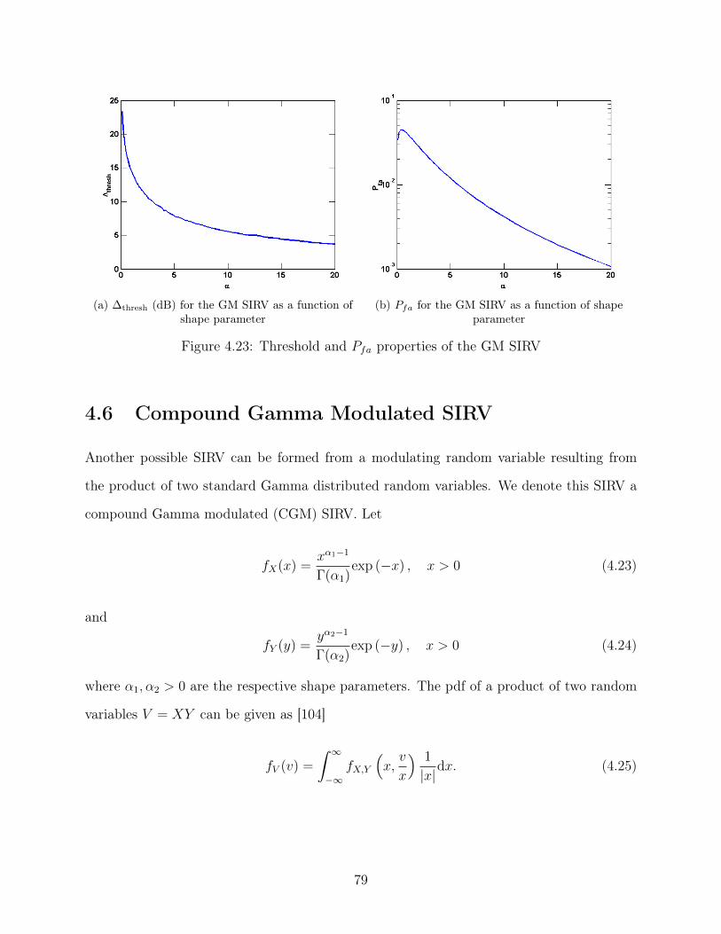
(a) ∆thresh (dB) for the GM SIRV as a function ofshape parameter
(b) Pfa for the GM SIRV as a function of shapeparameter
Figure 4.23: Threshold and Pfa properties of the GM SIRV
4.6 Compound Gamma Modulated SIRV
Another possible SIRV can be formed from a modulating random variable resulting from
the product of two standard Gamma distributed random variables. We denote this SIRV a
compound Gamma modulated (CGM) SIRV. Let
fX(x) =xα1−1
Γ(α1)exp (−x) , x > 0 (4.23)
and
fY (y) =yα2−1
Γ(α2)exp (−y) , x > 0 (4.24)
where α1, α2 > 0 are the respective shape parameters. The pdf of a product of two random
variables V = XY can be given as [104]
fV (v) =
∫ ∞−∞
fX,Y
(x,v
x
) 1
|x|dx. (4.25)
79

As X, Y > 0 and are independent, (4.25) becomes
fV (v) =
∫ ∞0
fX(x)fY
(vx
) 1
xdx
=
∫ ∞0
xα1−1
Γ(α1)exp (−x)
( vx)α2−1
Γ(α2)exp
(−(vx
)) 1
xdx
=
∫ ∞0
xα1−1x−α2+1vα2−1
Γ(α1)Γ(α2)exp
(−x−
(vx
)) 1
xdx
=
∫ ∞0
xα1−α2−1vα2−1
Γ(α1)Γ(α2)exp
(−x−
(vx
))dx. (4.26)
To simplify (4.26), first note that
fV (v) =
∫ ∞0
xα1−α2−1vα2−1
Γ(α1)Γ(α2)exp
(−x−
(vx
))dx
=vα2−1
Γ(α1)Γ(α2)
∫ ∞0
xα1−α2−1exp(−x−
(vx
))dx
=vα2−1
Γ(α1)Γ(α2)
2
2vα12−α1
2
∫ ∞0
xα1−α2−1exp(−x−
(vx
))dx
=2v
α2+α12−1
Γ(α1)Γ(α2)
vα2−α1
2
2
∫ ∞0
xα1−α2−1exp(−x−
(vx
))dx (4.27)
Next, recall (3.72), and let
β = α2 − α1
x = 2
z =√v (4.28)
80

leads to a modified Bessel function of the second kind of the form
Kβ(xz) =zβ
2
∫ ∞0
exp
[−x
2(t+
z2
t)
]t−β−1dt
=⇒ Kα2−α1(2√v) =
√vα2−α1
2
∫ ∞0
exp
[−2
2
(t+
v
t
)]t−(α2−α1)−1dt
=⇒ Kα2−α1(2√v) =
vα2−α1
2
2
∫ ∞0
exp[−t− v
t
]tα1−α2−1dt. (4.29)
Substituting (4.29) into (4.27) results in
fV (v) =2v
α2+α12−1
Γ(α1)Γ(α2)
vα2−α1
2
2
∫ ∞0
xα1−α2−1exp(−x−
(vx
))dx
=2v
α2+α12−1
Γ(α1)Γ(α2)Kα2−α1(2
√v). (4.30)
The similarity of (4.30) to (3.62) is unsurprising, as the K distribution is often derived as the
product of two correlated Gamma distributions, particularly in SAR applications (e.g. [83]
and references therein).
The function hL(q) is found by plugging the results of (4.30) into (3.10), yielding
hL(q) =
∫ ∞0
v−Lexp(− q
2v2)fV (v)dv
=
∫ ∞0
v−Lexp(− q
2v2
) 2vα2+α1
2−1
Γ(α1)Γ(α2)Kα2−α1(2
√v)dv
=2
Γ(α1)Γ(α2)
∫ ∞0
vα2+α1
2−L−1exp
(− q
2v2
)Kα2−α1(2
√v)dv. (4.31)
The pdf for real valued CGM SIRV data is then found from (3.11) and (4.31) to be
fQ(q) =1
2L2 Γ(L
2)qL2−1hL(q)
=qL2−1
2L2−1Γ(L
2)Γ(α1)Γ(α2)
∫ ∞0
vα2+α1
2−L−1exp
(− q
2v2
)Kα2−α1(2
√v)dv (4.32)
81

and the pdf for complex valued CGM SIRV data is
fQ(q) =qL−1
2L−1Γ(L)Γ(α1)Γ(α2)
∫ ∞0
vα2+α1
2−2L−1exp
(− q
2v2
)Kα2−α1(2
√v)dv (4.33)
We used Monte Carlo simulation to generate 106 instantiations of the CGM SIRV and
used a histogram to generate the cdf for the CGM SIRV for several shape parameters. For
illustrative purposes, we used identically distributed Gamma random variables (i.e. each
Gamma distribution has the same shape parameter). The cdf for the CGM SIRV is shown
in Figure 4.24 for shape parameters α1 = α2 = 1, 5, 50.
Figure 4.24: cdfs of the CGM SIRV distribution
Note the heavy tail of the CGM SIRV for low shape parameters. As the CGM SIRV
distribution is characterized by two shape parameters, we show the change in threshold
defined by (4.2) for varying values of α1 and α2 in Figure 4.25. Two features are apparent.
First, the threshold is maximized along the ridge defined by α1 = α2. As one holds α1
constant and increases α2 (or vice versa), the threshold decreases. Second, comparing Figure
4.23a to Figure 4.25, for arbitrary shape parameters the CGM SIRV appears to result in a
higher threshold than the GM SIRV.
82

Figure 4.25: ∆thresh (dB) for the CGM SIRV as a function of shape parameter
Figure 4.26 shows the Pfa for CGM clutter when the clutter is incorrectly assumed to be
Gaussian distributed. The threshold is derived from a desired Pfa = 10−6. For illustrative
purposes, we limit the plot to the α1 = α2 ridge, which was established to be the "worst
case" threshold via examination of Figure 4.25.
83

Figure 4.26: Pfa for the CGM SIRV as a function of shape parameter
4.7 Limitations of SIRVs
There have been multiple concerns raised about the utility of SIRVs in modeling non-
Gaussian radar clutter. First, care must be taken when generating simulated radar clut-
ter. For example, there has been recent work in modeling VHF SAR forest clutter with
SIRVs [105]. Due to the high range resolution of the SAR system, SIRV distributed scatter-
ers provide a good model to measured results. However, it was noted in [105] that the SAR
processing induced spatial correlation between range cells. A naive application of SIRV the-
ory can lead to simulated clutter that bears little similarity to measured results. Therefore,
both the spatial and temporal correlation must be accounted for in certain applications. The
problem of incorporating radar system sampling effects into clutter generation is outside the
scope of this work, but provides a promising area of future research.
Several members of the audience had constructive feedback after the presentation of [2].
There is some skepticism in the community as to the "fit" of measured data to the proposed
distributions. Recall that SIRVs are all related to the Gaussian distribution, and differ only
in distribution of the modulating random variable. Therefore, it is possible that there may
be ambiguities in terms of different SIRVs with respect to the tails of the distributions. This
concept of ambiguity between distributions is central throughout this work.
84

In a similar vein, most studies on fitting SIRV clutter focus on fitting measured data
to one or two known distributions. However, this parametric fitting of data presupposes
that the true distribution of the data comes from a set of known distributions. Therefore,
we ignore the possibility of an unknown distribution being the actual distribution of the
measured data. However, the SIRV model was shown in [7,46] to derive from a modification
of the central limit theorem based on the theory of electromagnetic scattering. Based on
this justification we may hypothesize that any unknown distributions may fit to the SIRV
class of random vectors. This line of reasoning raises the question of whether we can use
our knowledge of various SIRV distributions to successfully estimate the detection threshold
(i.e. tail) of an unknown distribution. After all, the purpose of using parametric models is
to maximize our probability of detection for a given false alarm rate. For the purposes of
a radar receiver, if a clutter model is incorrect, but yields a correct threshold, any system
using the output of the detector (e.g. tracker, target identifier) does not care about the
distribution used by the detector. This theme will be explored in more detail in Chapters
6-8.
85

Chapter 5
Distribution Estimation using
Combinations of Order Statistics
This chapter examines the use of ordered statistics to explore both parametric and non-
parametric distribution identification techniques. Consider N variables, X1, . . . , XN , which
are assumed to be IID with pdf fX(x). The ordered statistics X(1), . . . , X(N) are formed by
sorting the random variables by increasing magnitude as [106]
X(1) ≤ X(2) ≤ · · · ≤ X(N). (5.1)
Individual order statistics are often used in many non-parametric and parametric applica-
tions. For example, the minimum (X(1)), maximum (X(N)), and median (X(N/2)) are often
used to provide context to sampled data. The pdf of the ith order statistic from a distribution
with cdf F (x) is given as
f(i)(x) =1
B(i, n− i+ 1)F i−1(x)[1− F (x)]n−if(x) (5.2)
86

where B(a, b) is the Beta function defined as
B(a, b) =
∫ 1
0
ta−1(1− t)b−1dt a > 0, b > 0. (5.3)
Order statistics are often invoked to provide robustness to data processing techniques,
especially with respect to outliers in measured data [107]. For example, the median filter
(i.e. the output of the filter is the median of a sliding window of data) is effective at smooth-
ing data but preserves edges or impulses better than conventional low pass finite impulse
response (FIR) filters [108], [107, Chapter 21]. Radar signal processing engineers have long
used order statistics in various ways to reduce false alarms (e.g. [42], [107, Chapter 23]).
The remainder of this chapter is concerned with the application of order statistics for dis-
tribution identification of non-Gaussian radar clutter. The first section explores a prior
technique known as the Ozturk algorithm, and we apply the algorithm to measured radar
data. The subsequent sections provide our extensions to the Ozturk algorithm and explore
their applicability to radar signal processing. Finally, we culminate in a proposed design to
fuse multiple test statistics with the goal of classifying an underlying clutter statistic and
adaptively estimating a detection threshold.
5.1 The Ozturk Goodness-of-Fit Algorithm
Goodness-of-fit algorithms are a class of techniques that determine whether measured data
fits hypothesized distributions. Classical order statistic based techniques use quantiles of the
cdf of a distribution, or require the hypothesized distributions to be of the location/scale
type [107, Chapter 16]. For the latter methods, the distributions may be discriminated
by the actual locations of the individual order statistics or the spacing between the order
statistics [107, Chapter 17].
A graphical goodness-of-fit algorithm based on ordered statistics was developed in a series
of papers [109–112] and refined to consider SIRV clutter in [1]. This algorithm will be denoted
87

as the Ozturk alorithm for the remainder of this work. Originally, the Ozturk algorithm
was developed to assess the normality (i.e. Gaussianity) of a distribution. In subsequent
developments, the Ozturk algorithm was altered to provide a method of efficiently comparing
sampled data to a library of known distributions and determining the distribution that the
sampled data most closely resembles. This section describes the method and reasoning
behind the Ozturk algorithm. The intuition gathered from this algorithm gives rise to the
novel methods presented and tested in the subsequent sections.
The Ozturk algorithm uses the Gaussian distribution as the null hypothesis and attempts
to develop a distance measure on a two dimensional space relative to the Gaussian distribu-
tion for a group of other distributions. Therefore, measured data could be easily (i.e. with
low computational cost) projected onto this space and the nearest known point determined.
A key benefit of this approach is to change the distribution identification problem from a
hypothesis test to a hypothesis suggestion. Recall that SIRV distributions are all Gaussian
distributions that have been modulated by a random variable. Therefore, the fact that the
Ozturk algorithm attempts to measure distance between a candidate distribution and the
Gaussian distribution indicates that it may be well suited to identifying SIRV distributions.
To implement the Ozturk algorithm, one constructs a set of vectors associated with the
order statistics of a distribution. As the algorithm operates in two dimensions, denoted as
U and V , each vector may be described by a magnitude and angle. The set of angles φi used
are common to all distributions. However, the magnitude of each vector is generated from
the studentized order statistics [106] of the individual distribution. These vectors are then
linked head-to-tail. The endpoint of the linked vectors is the discriminating statistic of the
algorithm.
To develop the vector magnitudes of a SIRV distribution, consider a series of N sampled,
zero mean, independent and identically distributed (i.i.d.) length L vectors y1,y2, . . .yN
88

with covariance Σ and the corresponding quadratic forms
q1 = yH1 Σ−1y1
q2 = yH2 Σ−1y2
...
qN = yHNΣ−1yN . (5.4)
The quadratic samples are then sorted as
q(1) ≤ q(2) ≤ · · · ≤ q(N). (5.5)
The sample mean of the quadratic samples is found as
q̄ =1
N
N∑i=1
qi (5.6)
and the sample variance of the quadratic samples is
σ̂2 =1
N − 1
N∑i=1
(qi − q̄)2. (5.7)
The studentized order statistics are obtained as [106]
z(i) =q(i) − q̄σ̂
(5.8)
In other words, studentization enforces a zero mean, unit variance constraint on the sampled
data.
To create angles φ1, φ2, . . . φN , the Ozturk algorithm uses the expected value of the N
89

order statistics of the standard Normal distribution given as
m(i) = E[x(i)], i = 1, . . . , N (5.9)
where x ∼ N (0, 1). The angles φ1, φ2, . . . φN are then generated as
φi = πΦ(m(i)), i = 1, . . . , N (5.10)
where Φ(•) is the cdf of the standard normal distribution.
Finally, the vectors whose length is given by |z(i)| and whose angle with respect to the
V axis is φi are linked. Starting at (0, 0), the coordinates of the endpoint of each vector is
given by
Uk =1
k
k∑i=1
cos(φi)|z(i)|
Vk =1
k
k∑i=1
sin(φi)|z(i)|
k = 1, . . . , N. (5.11)
The endpoint (UN , VN) for each distribution is then plotted. Figure 5.1 illustrates the Ozturk
algorithm for a candidate distribution and the null (Gaussian) distribution.
90

Figure 5.1: Illustration of linked vectors (reprinted from [1])
Note that the number of data points used to form the order statistics must be known a
priori. However, it is possible to form a library of distribution plots offline to be deployed
according to need. An example library was generated in [1]. A visual representation of the
library is shown in Figure 5.2.
91

Figure 5.2: Library of endpoints for SIRV identification (reprinted from [1])
The lines in Figure 5.2 are formed by distributions with shape parameters. Note that
all distributions converge to the Gaussian distribution on the right for some value of their
shape parameter (i.e. ν = 2 for the Weibull distribution and ν =∞ for the K distribution).
The Ozturk algorithm was implemented and tested in a Monte Carlo fashion on real val-
ued K distributed SIRV data. Each length L = 16 SIRV was given a zero mean vector and
covariance matrix structured so that σ2yiyj
= E[YiYj]2 = L−|i−j|
L(i.e. linearly decreasing co-
variance). There were N = 16 samples to generate the ordered statistics, and 100,000 Monte
92

Carlo runs were performed. Figure 5.3a shows the null distribution and the K distribution
for shape parameters ν = 0.5, 1.
(a) Ozturk algorithm example library (b) Graphical pdf of K endpoint distribution
Figure 5.3: Implementation of the Ozturk algorithm
Each circle of Figure 5.3a corresponds to the average endpoints generated for each linked
vector. Figure 5.3b shows the distribution of the endpoint of a K distributed variable with
shape parameter ν = 1. Unlike the other figures, 200,000 Monte Carlo simulations were run
to generate Figure 5.3b, but all other pertinent variables were held constant. The pdf is
given in 10log10(fU,V (u, v)).
It was asserted in [1] that the Ozturk algorithm was scale invariant. Due to the non-
ergodicity of a SIRV (caused by the modulating random variable), the true covariance matrix
and the sample covariance matrix of a SIRV will differ by a scale factor [75]. The scaling factor
will tend toward unity as the number of samples used to construct the sample covariance
matrix goes to infinity. The property of scale invariance allows the Ozturk algorithm to be
well suited to identifying SIRV distributions from limited data samples. Figures 5.4a and
5.4b illustrate the scale invariance of the Ozturk algorithm.
93

(a) Sample cov. matrix v. true cov. matrix (b) Effect of increasing sample size
Figure 5.4a shows the linked vectors generated when the true covariance matrix is known,
and whenK = 16L = 256 vectors were used to generate the sample covariance matrix. Figure
5.4b shows the effect of increasing the number of samples used to estimate the covariance
matrix. Notice that while using K = L = 16 sample vectors does not appear to produce
accurate results, the endpoint for K = 4L and K = 16L sample vectors produce very similar
results. Therefore, the Ozturk algorithm should perform well even with limited sample
support. Note in practical STAP systems, the Reed, Mallett, Brennan (RMB) rule states
that a system will suffer a detection loss of approximately 3 dB if K = 2L samples are used
to estimate the sample covariance matrix [47]. The RMB rule will be explored in future
work.
5.1.1 Applying the Ozturk Algorithm
As a proof of concept, we implemented the Ozturk algorithm with an initial library consisting
of the K distribution and the Gaussian distribution (i.e. the null hypothesis in terms of dis-
tribution identification). These average endpoints are then compared to measured endpoints
from the multichannel airborne radar measurement (MCARM) program [113]. The MCARM
program used an L band radar operating at 1240 MHz. The MCARM radar transmits a
50.4 µs linear frequency modulated waveform with a pulse compression ratio of 63. This
94

waveform is transmitted from an 11 × 11 planar array mounted on the side of a BAC1-11
aircraft. For further details on the MCARM program, see [75, 113–115] and the references
contained therein.
While multiple channels of data are provided by the MCARM data files, this early imple-
mentation of the Ozturk algorithm does not support data from multiple antennas. Therefore,
for this proof of concept we only consider the data from the first antenna. We implemented
the Ozturk algorithm for the complex Gaussian distribution as well as complex K distributed
data, with shape parameter 0.3 ≤ ν ≤ 4 by steps of 0.1. The MCARM data files provide
measurements for a coherent processing interval of 128 pulses and 630 range cells. For this
initial implementation we divide the measurements of each range cell into 8 measurements
of L = 16 consecutive pulses. A sliding window is formed consisting of 10 range cells, for a
sample matrix of dimension 16 × 80. The sample covariance matrix is estimated from this
K × 5L matrix. The 80 vectors are "compressed" into their quadratic using the inverse of
the sample covariance matrix. The endpoint is formed as discussed in Section 5.1. Each new
endpoint is formed by sliding the window one range cell farther from the radar, until the
final range cell is reached.
Figure 5.5 shows the output of the Ozturk algorithm when applied to MCARM data file
rd050465. The blue line shows the path formed by endpoints of K distributed data. Notice
that the shape parameter of the K distribution is increasing smoothly from left to right,
and tends toward the Gaussian endpoint at the far right. The individual circles represent
endpoints of the Ozturk algorithm as applied to the sliding window. This experiment serves
as a conceptual illustration of the Ozturk algorithm, and establishes the applicability of the
Ozturk algorithm to real data.
95

Figure 5.5: Implementation of Ozturk algorithm on MCARM data file rd050465
In the future we will modify the assumption of 8 individual SIRVs per CPI. The "sam-
pling" rate of the modulating variable will be allowed to vary. Further, Figure 5.5 shows the
need to expand the library of SIRVs from the K distribution. We will investigate the expan-
sion of the library, as well as the expansion of the basic principles of the Ozturk algorithm,
in the subsequent sections.
5.2 Weighted Sums of Ordered Statistics
In this section we expand on the Ozturk algorithm and generalize it by introducing a new
framework of combining ordered statistics through weighted sums. Most of the reasoning
in this section is focused on development of intuition for the Ozturk algorithm, as well as
96

extending this intuition to new methods. The Ozturk algorithm was developed to provide a
one-to-one mapping from the space of order statistics to a two-dimensional space. This space
was designed to provide a distance metric between distributions. While not addressed in the
publications, clearly such a strategy wishes to maximize the distance between distributions
in order to provide an accurate classifier. Here we introduce new weighting functions, and
consider the use of non-studentized data. Finally, we address the applicability of identifying
distributions with limited sample support and the correlation between the sums given by
different weighting functions.
It should be noted that for the Ozturk algorithm, the endpoint of the linked vectors
provides the discriminating data point of interest. Throughout this work we continue to use
this terminology, despite removing the vector notation and intuition established in Section
5.1. First, we use this notation for consistencies sake. Second, in future work we will revisit
the physical interpretation of linked vectors in a modified form. The future work is discussed
in section 9.2.
Define a weighted sum of ordered statistics (WSOS) as
U(X) =N∑i=1
aiX(i). (5.12)
If the ordered statistics are not first studentized, (5.11) becomes a special case of (5.12).
Upon closer inspection of (5.10), the expectation yields
φi = πΦ(m(i)), i = 1, . . . , N
= πi
N + 1, i = 1, . . . , N. (5.13)
In other words, the series φ1, . . . , φN corresponds to a uniform sampling of (0, π). Therefore,
the weightings in (5.11) correspond to a cosine weighting and a sine weighting with argument
given by the series (5.13).
For the Ozturk algorithm, the quadratic values have been studentized. As the ordered
97

statistics are positive before studentizing, the minimum values will tend towards the negative
of the mean of the quadratic values, scaled by the square root of their variance. However, the
Ozturk algorithm takes the magnitude of the studentized statistics, causing the new values
associated with the minimum measured values to become positive, yet close to the scaled
mean. Similarly, the statistics that were close to the mean will be close to zero.
This exploration causes one to consider the selection of the sine and cosine as weightings.
With an argument uniformly distributed (0, π), the sine function provides very low weights
to extreme values of the distribution (i.e. order statistics near the minimum and maximum
are weighted close to zero). However, the values near the median are weighted strongly.
Therefore, the sine function at this interval emphasizes the median values and deemphasizes
the values at the tails of the distribution. An example of sine weightings is shown in Figure
5.6a. For the Ozturk algorithm, this weighting will provide information to the difference
between the mean and the median of a distribution. If the data is not studentized, the sine
appears to simply emphasize the median values.
However, the cosine function over the same interval gives positive weight to minimum val-
ues, negative weight to maximum values, and very little weight to statistics near the median
of the distribution. The cosine weighting, as applied in the Ozturk algorithm, would appear
to provide a measure of the separation between the mean and the tails of a distribution.
Just as using both weightings of studentized and non-studentized order statistics provide
two different data points for each observation, increasing the number of weightings consid-
ered can cast the distribution identification problem into a higher order dimensional space.
Therefore, it becomes instructive to examine different possible weightings.
Figure 5.6a shows the weights supplied by using a uniform spacing of the open interval
(0, 1) parameterized by the variable t. As mentioned previously, the sine weights provide
smaller weight to the extremes of the ordered samples symmetrically around the median.
However, the sine squared weightings provide even less weight to the samples farther from
the median. In other words, the shaping is sharper around the median.
98
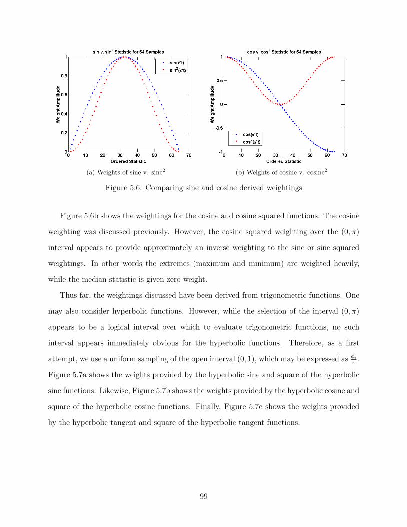
(a) Weights of sine v. sine2 (b) Weights of cosine v. cosine2
Figure 5.6: Comparing sine and cosine derived weightings
Figure 5.6b shows the weightings for the cosine and cosine squared functions. The cosine
weighting was discussed previously. However, the cosine squared weighting over the (0, π)
interval appears to provide approximately an inverse weighting to the sine or sine squared
weightings. In other words the extremes (maximum and minimum) are weighted heavily,
while the median statistic is given zero weight.
Thus far, the weightings discussed have been derived from trigonometric functions. One
may also consider hyperbolic functions. However, while the selection of the interval (0, π)
appears to be a logical interval over which to evaluate trigonometric functions, no such
interval appears immediately obvious for the hyperbolic functions. Therefore, as a first
attempt, we use a uniform sampling of the open interval (0, 1), which may be expressed as φiπ.
Figure 5.7a shows the weights provided by the hyperbolic sine and square of the hyperbolic
sine functions. Likewise, Figure 5.7b shows the weights provided by the hyperbolic cosine and
square of the hyperbolic cosine functions. Finally, Figure 5.7c shows the weights provided
by the hyperbolic tangent and square of the hyperbolic tangent functions.
99

(a) Weights of sinh v. sinh squared (b) Weights of cosh v. cosh squared
(c) Weights of tanh v. tanh squared
Figure 5.7: Comparing sinh, cosh, and tanh derived weightings
While the shape of the curve corresponding to each weighting function is different, all the
weightings for the hyperbolic function provide increasing weights as the order of the statistic
increases. While the weightings for the trigonometric functions are all bound −1 ≤ ai ≤ 1, no
such strict bounding is common to all hyperbolic functions. It may be necessary to consider
normalization procedures when hyperbolic functions are used to generate weightings.
In order to explore the weighting schemes presented, consider the order statistics formed
by examining instantiations of a dimension L = 64 complex K distributed SIRV with shape
parameter ν = 1 and scale parameter b = 1.5. The simulated pdf and cdf of the quadratic
form q of this random vector is shown in Figures 5.8a and 5.8b. Note that unless the Ozturk
100

method is specified, all figures in this section make use of non-studentized order statistics,
and no normalization is performed on any of the endpoint statistics.
(a) pdf of K Distributed SIRV withL = 64, ν = 1, b = 1.5
(b) cdf of K Distributed SIRV withL = 64, ν = 1, b = 1.5
Figure 5.8: pdf and cdf of example K distributed SIRV
Clearly, the number of samples N used to form ordered statistics will influence the final
value of the weighted sum. It is expected that as the number of samples increases, the better
approximation to the underlying quadratic PDF will be given. Therefore, the variance of
the WSOS should be lower and the separation between the endpoints of different weighting
methods should be greater. Note that in practiceN samples are used to estimate the common
covariance matrix Σ̂. Therefore, for a full rank estimation of the covariance matrix, in a
general application it is common to require N ≥ L.
First, Figures 5.9a and 5.10b considers the sine and sine squared weightings for N =
L, 4L = 64, 256.
101

(a) N = L (b) N = 4L
Figure 5.9: Endpoint distribution for sin and sin2
The histogram of the WSOS for each of these weightings is shown. Examining Figure
5.6a, the two weighting functions are of similar and weight the median value identically.
Therefore, it is expected that the pdfs of these WSOS overlap a great deal. However, when
the number of samples is increased to N = 4L = 256, the pdfs are well separated.
Next Figures 5.10a and 5.10b examine the cosine and cosine squared weightings
(a) N = L (b) N = 4L
Figure 5.10: Endpoint distribution for cos and cos2
While it is not immediately obvious from Figure 5.6b, these two pdfs do not appear well
separated for N = L. However, just as with the sine and sine squared WSOS pdfs, increasing
102

the number of samples allows one to clearly discriminate between the two pdfs.
The hyperbolic cosh and tanh functions, along with their respective squares, appear to
provide well separated WSOS. This separation is illustrated in Figures 5.11a through 5.11d.
(a) N = L (b) N = 4L
(c) N = L (d) N = 4L
Figure 5.11: Endpoint distribution for cosh, cosh2, tanh, and tanh2
However, the sinh and sinh squared functions do not appear to be well separated, as
shown in Figures 5.12a and 5.12b.
103

(a) N = L (b) N = 4L
Figure 5.12: Endpoint distribution for sinh and sinh2
While examining the univariate distributions of the WSOS is illustrative, it is also in-
structive to examine the bivariate distribution for pairs of WSOS. Figures 5.13a through
5.13d show the bivariate distributions of four pairs of WSOS for the N = L case.
104

(a) Endpoint distribution of cos and sin WSOS (b) Endpoint distribution of cos2 and sin2 WSOS
(c) Endpoint distribution of cosh and sinh WSOS (d) Endpoint distribution of cos and cosh2 WSOS
Figure 5.13: Endpoint distributions for pairs of weighting functions with K distributed data
Note that Figure 5.13a is equivalent to the Ozturk algorithm except for the scaling factor
1N
and the lack of studentization. The ridge in Figure 5.13a shows some correlation between
the cosine and sine weightings. However, Figure 5.13b appears to have much less correlation
between the two functions. This lack of correlation could be predicted from Figures 5.6a
and 5.6b, where the cosine squared and sine squared weightings appear to weight opposite
areas of the pdf highly. Therefore, the cosine squared and sine squared weightings used in
conjunction should be better at identifying K distributed data using the WSOS method than
if they were used separately. In addition, of the four pairings considered here, they appear to
yield the most information. Notice that the cosh and sinh WSOS are very highly correlated.
105

Finally, the cosine and cosh squared weightings appear to have a similar distribution to the
cosine and sine WSOS.
This section explored a generalized form of the Ozturk algorithm with non-studentized
data. The weighting functions were expanded to additional trigonometric and hyperbolic
functions in an effort to provide diversity. Finally, the correlation between WSOS for different
weighting functions was shown.
5.3 Scaled Weighted Sums of Ordered Statistics
Section 5.2 generalized the Ozturk algorithm to a weighted sum of ordered statistics with
non-studentized data. Now we propose a new set of weighted sums of ordered statistics
(WSOS) that are scaled based on the sampled data. These new methods are the studentized
WSOS, the divide by mean (DBM) WSOS, and an extension of the Ozturk algorithm to
arbitrary weightings, denoted as the extended Ozturk algorithm (EOA).
Note from (5.8) the data is studentized by subtracting the sample mean and scaling
the result by the sample standard deviation. Therefore, the studentized order statistics are
forced to zero mean, unit variance. In (5.11), the Ozturk algorithm takes the additional step
of taking the absolute value of the resulting order statistics. In the context of the Ozturk
algorithm, this step corresponds to assigning the magnitude of a vector. We propose using
the studentized order statistics without taking the absolute value.
We re-define the Ozturk order statistics as
zOz,(i) =
∣∣∣∣q(i) − q̄σ̂
∣∣∣∣ (5.14)
where q(i) are the ordered, quadratic samples defined in (5.5), q̄ is the sample mean of the
quadratic samples defined in (5.6), and σ̂ is the sample standard deviation defined in (5.7).
106

The studentized order statistics are denoted as
zStud,(i) =q(i) − q̄σ̂
. (5.15)
Noting that the quadratic samples qi are power estimates, we take inspiration from the
classic CFAR detector and propose scaling the order statistics by the sample mean [42]. The
divide by mean (DBM) order statistics are defined as
zDBM,(i) =q(i)
q̄. (5.16)
The three variants of scaled WSOS can then be formed from the 10 proposed weighting
functions given in Section 5.2 and the three scaled order statistics given in (5.14), (5.15),
and (5.16). The general WSOS given in Section 5.2 may be thought of as a constant scaling
of 1 over all samples.
5.4 Combined Order Statistics Modeled in Clutter
The methods presented in this chapter are based on a general statistical premise: determining
the underlying distribution of sampled SIRV data. However, in the context of radar detection,
the underlying distribution of clutter is by definition a means to an end: the detection of a
target with a constant, predictable probability of false alarm. The threshold for detection is
determined from the tail of the clutter distribution. Therefore, we examine the possibility of
mapping directly from endpoint space to a detection threshold for each of the four frameworks
discussed.
Recalling the characteristics of [4], by modeling the radar clutter as a SIRV we have
used the principle of prior information. Using the sample covariance matrix with small
sample support allows the methods we have presented to adapt to temporal non-stationarities
between coherent processing intervals. The remainder of this section will emphasize the
107

principle of robustness. By using multiple scalings and weighting functions, we provide
a diverse range of possible endpoints. As we are attempting to model clutter, and use a
framework of combinations of order statistics to determine the clutter distribution and/or
a detection threshold, we denote the combined algorithm the Combined Order Statistics
Modeled in Clutter (COSMiC) algorithm.
In the spirit of the Ozturk algorithm, we examine the correlation between endpoints for
several pairs of weightings for each of the scaled WSOS and the non-scaled WSOS. Then, we
examine the thresholds for each expected endpoint location. Clearly, for the purposes of radar
detection we desire a one-to-one (i.e. bijective) mapping between endpoint and detection
threshold. The threshold "space" will be quantified by the change in threshold with respect
to Gaussian distributed clutter. This quantification is calculated via (4.2). By looking at
pairs of endpoints we increase measurement diversity and introduce the possibility of two
beneficial yet differing goals. First, if the location of the endpoints for two different functions
are tightly correlated (i.e. the location of the endpoint for one weighting function tells us
where the endpoint will land for a different weighting function), those weighting functions and
the corresponding weighting algorithm are good candidates for a robust estimator. However,
if the average endpoints are in each weighting "space" are different as a function of source
(SIRV) distribution, the algorithm (e.g. WSOS, DBM, Studentized, EOA) and weighting
functions used are good candidates for a distribution classifier. This second goal was the
goal of the original Ozturk algorithm. The distinction between these two goals, as well as
candidate methods for each goal, are examined in this section.
In general, the COSMiC goals may be expressed via the flowcharts shown in Figures
5.14a and 5.14b.
108
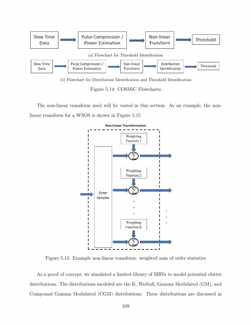
(a) Flowchart for Threshold Identification
(b) Flowchart for Distribution Identification and Threshold Identification
Figure 5.14: COSMiC Flowcharts
The non-linear transform used will be varied in this section. As an example, the non-
linear transform for a WSOS is shown in Figure 5.15
Figure 5.15: Example non-linear transform: weighted sum of order statistics
As a proof of concept, we simulated a limited library of SIRVs to model potential clutter
distributions. The distributions modeled are the K, Weibull, Gamma Modulated (GM), and
Compound Gamma Modulated (CGM) distributions. These distributions are discussed in
109

detail in Chapters 3 and 4. Each endpoint was found through Monte Carlo simulation of
106 complex SIRVs, each of dimension L = 4. We use N = 4L = 16 order statistics of
the quadratic form of the SIRV to form each endpoint. The clairvoyantly known covariance
matrix was used to form each quadratic sample. The thresholds were all found by Monte
Carlo simulation of 108 quadratic samples of the SIRV, with a desired Pfa = 10−6. In forming
all WSOS, we divide the final sum (i.e. endpoint) by N to reduce the scale of the endpoint
space, and provide continuity to the previous work in [1, 109–112].
In this section we denote the "best" weighting function/algorithm combinations to be the
mappings with the least ambiguities. We examine two types of plots. First, we look at the
relation of the average endpoint locations for pairs of weighting functions. The endpoints
are parametrized twice. First, they are parametrized by distribution (the four previously
mentioned). Second, each distribution is parametrized by shape parameter(s). For a robust
estimator, the two dimensional endpoints will ideally trace either a straight line or a curve
with little to no variance. For a distribution classifier, the endpoints should trace separate
"paths" of endpoints. Each of these paths should consist of points from a single distribution
with a varying shape parameter. Note that points from multiple paths could share a common
threshold (i.e. distribution tail). The second type of plot is a mapping from "endpoint space"
to "threshold space". In other words, for each of the distributions simulated we estimated
the change in threshold for a CFAR radar above the threshold one would use in Gaussian
clutter. For each weighting function/algorithm pair examined we then plot the endpoints of
each distribution with respect to the change in threshold. A "good" mapping is one where
distributions with similar endpoints also possess similar thresholds. If a point in endpoint
space corresponds to multiple thresholds, there is an ambiguity at that location in endpoint
space. A "tight" mapping is considered to be a point in endpoint space where the difference
in threshold for close points is on the order of ε dB, where ε is defined by the user. The
concepts of "good" pairs of weighting functions and processing algorithms will be examined
in the context of the plots given in the rest of this section.
110

To begin, Figures 5.16a-5.16d examine examine the sine and cosine pairing. As mentioned
previously, each endpoint corresponds to one of four distributions with a varying shape
parameter (and threshold). Figure 5.16a shows the library of average endpoints for the
WSOS algorithm. For the WSOS algorithm with sine and cosine weighting functions, the
path of the endpoints for the distributions in this library appear to trace an arc from left
to right (i.e. lower values of the each endpoint correspond to distributions with greater
thresholds). The top right endpoint is equivalent to the Gaussian distribution (Weibull with
shape ν = 2). The sine and cosine functions appear to correlate fairly tightly, but there is
variance around the arc traced. The variance appears to be primarily caused by the Weibull
distributed values. Therefore, the WSOS algorithm with sine and cosine weightings is a
candidate for a robust estimator to determine the threshold for SIRV data. Depending on
the variance in endpoint values, it may also be a candidate to determine whether sample
data fits a Weibull distribution or a SIRV distribution derived from a transformed Gamma
modulating random variable (e.g. K, GM, CGM).
111

(a) Endpoint distribution of cosine and sine WSOS(b) Endpoint distribution of cosine and sine DBM
WSOS
(c) Endpoint distribution of cosine and sineStudentized WSOS (d) Endpoint distribution of cosine and sine EOA
Figure 5.16: COSMiC endpoint distributions, cosine v. sine
Figure 5.16b shows the endpoint distribution for the DBM algorithm with the sine and
cosine function weightings. The endpoint arc and slight variance appear similar to the results
for the WSOS algorithm shown in Figure 5.16a. Therefore, the DBMmethod andWSOS may
be used in tandem to produce a robust estimate. Figure 5.16c shows the endpoint distribution
for the Studentized WSOS using the sine and cosine weighting functions. Unlike the WSOS
and DBM methods, the Studentized method produces endpoints with increasing thresholds
corresponding to decreasing sine values and increasing cosine values. The Gaussian threshold
is at the top left of the arc. In addition, the endpoint distribution has an ambiguity when
112

the sine weighting function is used. Because of this ambiguity, the Studentized WSOS with
the sine weighting function may not a good candidate to explore or exploit compared to the
methods explored in this analysis. Figure 5.16d gives a library of endpoints corresponding
to the original Ozturk algorithm. Unlike the other three methods, the EOA provides a clear
distinction between the individual distributions making up the library. However, this implies
that the EOA may not yield a bijective mapping from endpoint space to threshold space.
Next we examine the individual endpoints given by the cosine weighting function and
the corresponding changes in thresholds.
(a) Endpoint distribution of cosine v. threshold forWSOS
(b) Endpoint distribution of cosine v. threshold forDBM WSOS
(c) Endpoint distribution of cosine v. threshold forStudentized WSOS
(d) Endpoint distribution of cosine v. threshold forEOA
Figure 5.17: COSMiC endpoint distributions for cosine v. threshold
113

It is immediately apparent that there are ambiguities between the endpoint space and the
∆thresh for all methods. In other words, points falling close to each other in endpoint space
correspond to distributions with very different tails (and therefore different thresholds). In
the context of the radar detection problem, this ambiguity is problematic. However, as a
practical matter, in this work we concentrate on changes in threshold less than 10 dB. As
the threshold has a direct relation to the probability of detecting a target when a target is
present, a 10 dB loss of detection will likely compromise the functionality of a typical radar.
In future work, we will examine the endpoint location of measured radar data. If these
measurements suggest higher thresholds are needed, the limit of a 10 dB change in threshold
will be re-examined.
Figure 5.18: Ambiguity for cosine v. threshold
Figure 5.17a shows the cosine endpoint and the corresponding change in threshold for
the WSOS method. The ambiguity in Figure 5.17a is highlighted in Figure 5.18. Figure
5.17b shows the cosine endpoint and change in threshold for the DBM method. As with
Figures 5.16a and 5.16b suggest, the results for the WSOS and DBM methods are similar
up to a scaling factor for the endpoint. Intuitively, this makes sense as the divide by mean
(DBM) method is dividing by the mean of a series of power estimates arising from identically
distributed data. Therefore, in the expectation, these points should be identical up to a
114

scale factor. However, in practice this scaling may prove to make the estimate more robust.
The robustness of the DBM method, and the improvement offered by combining the two
methods, will be explored in future work. Similarity aside, neither the WSOS nor DBM
method appears to provide an unambiguous mapping into threshold space with the cosine
weighting function. However, for changes in threshold below 5 dB, the Studentized WSOS
and EOA provide a tight mapping between cosine endpoint space and threshold space.
Next, Figures 5.19a-5.19d show the relation between the sine endpoint and the change
in threshold for the four methods. Figures 5.19a and 5.19b illustrate the scaling difference
between the WSOS and the DBM methods. However, unlike the cosine endpoint, the map-
ping between sine endpoint space and threshold space appears to be tight for low changes
in threshold (∆thresh < 5 dB). Figure 5.19c gives the mapping between sine endpoint space
and the change in threshold for the Studentized WSOS method. The ambiguity shown in
Figure 5.16c is apparent in Figure 5.19c. However, the ambiguous endpoints are in the end-
point space we are not interested in. In addition, the mapping between endpoint space is
tight for values ∆thresh < 5. Figure 5.19d shows the results for the sine endpoint when the
EOA is used. When the modulating random variable of the underlying SIRV distribution
is derived from the Gamma distribution (i.e. K distribution, GM, CGM), there is a tight
mapping from sine endpoint space to values of ∆thresh < 11 dB. However, the sine endpoint
ambiguously maps to a higher threshold for a Weibull distributed SIRV than for the Gamma
derived SIRVs.
Therefore, when combining the sine and cosine weightings the EOA (in this case identical
to the original Ozturk algorithm) provides the best distribution discrimination. For the
individual endpoints, the Studentized WSOS and EOA methods provide the best (least
ambiguous) mapping into the threshold space.
115

(a) Endpoint distribution of sine v. threshold forWSOS
(b) Endpoint distribution of sine v. threshold forDBM WSOS
(c) Endpoint distribution of sine v. threshold forStudentized WSOS
(d) Endpoint distribution of sine v. threshold forEOA
Figure 5.19: COSMiC endpoint distributions for sine v. threshold
Next, we examine the combination of the sine squared and cosine squared weighting
functions for the four methods. Figures 5.20a and 5.20b show results of the WSOS and
DBM methods, respectively. As expected, they differ only by a scale factor. There appears
to be a linear, perfectly correlated relationship between the cosine squared endpoint and the
sine squared endpoint for the WSOS and DBM methods.
116

(a) Endpoint distribution of cosine squared and sinesquared WSOS
(b) Endpoint distribution of cosine squared and sinesquared DBM WSOS
(c) Endpoint distribution of cosine squared and sinesquared Studentized WSOS
(d) Endpoint distribution of cosine squared and sinesquared EOA
Figure 5.20: COSMiC endpoint distributions, sine squared v. cosine squared
Like the WSOS and DBM methods, Figure 5.20c shows that the Studentized WSOS
method also results in a linear, perfectly correlated relationship between the sine squared
weighting function and the cosine squared weighting function. In addition, visual inspection
of the upper left of the endpoint space (i.e. the largest sine squared values and smallest
cosine squared values) shows that in this case the distributions with lower thresholds are
"spread" out. In other words, for samples produced by a K distribution or Weibull distribu-
tion with large shape values the cosine squared and sine squared weighting functions used
in conjunction with the Studentized WSOS method separate the endpoints. However, the
117

Weibull and K endpoints are still interspersed, so this method may not be used to distin-
guish between distributions. However, Figure 5.20d shows the distribution discrimination
capabilities of the Ozturk algorithm apply to the new weighting functions.
Figures 5.21a-5.21d show the cosine squared endpoint with respect to change in threshold
for the four methods. Examining Figures 5.21a and 5.21b, the cosine squared weighting
function does not appear to be better than cosine weighting function or sine weighting
function at determining threshold unambigously when the WSOS or DBM methods are
used.
(a) Endpoint distribution of cosine squared v.threshold for WSOS
(b) Endpoint distribution of cosine squared v.threshold for DBM WSOS
(c) Endpoint distribution of cosine squared v.threshold for Studentized WSOS
(d) Endpoint distribution of cosine squared v.threshold for EOA
Figure 5.21: COSMiC endpoint distributions for cosine squared v. threshold
118

However, the Studentized WSOS method, as shown in Figure 5.21c, produces a similar
ambiguity for high threshold distributions as was seen for the sine weighting function was
used for the same method. The StudentizedWSOS method with the cosine squared weighting
function gives a tight approximation of the threshold for ∆thresh < 5 dB. The spreading of low
threshold distributions is also apparent in Figure 5.21c. As the Weibull and K distribution
are both commonly measured, the pairing of the cosine squared weighting function and the
Studentized WSOS is a promising technique and will be investigated further with measured
data. Figure 5.21d shows the effectiveness of the EOA method for mapping distributions
with ∆thresh < 8 dB to an endpoint generated with the cosine squared weighting function.
Figures 5.22a-5.22d show the change in threshold when the sine squared weighting func-
tion is used for the four different methods. By comparing Figures 5.22a-5.22c to Figures
5.21a-5.21c, the suitability of the sine squared weighting function in mapping from end-
point space to threshold space appears to be approximately equivalent to the cosine squared
threshold for the WSOS, DBM, and Studentized WSOS methods. For both weighting func-
tions the mapping appears to have have a low amount of ambiguity for ∆thresh < 5. Unlike
the cosine squared weighting function, higher threshold distributions map to smaller valued
endpoints when the sine squared weighting function is used (i.e. the "direction" of travel
when increasing threshold is reversed). Also, as can be seen in Figures 5.22c and 5.21c,
the ambiguity for high threshold distributions appears to be complimentary to the cosine
squared weighting when the Studentized WSOS method is used. As a result, the ambiguity
is identically "folded" into the line of endpoints seen in Figure 5.20c when the cosine squared
and sine squared weighting functions are used in conjunction.
119

(a) Endpoint distribution of sine squared v.threshold for WSOS
(b) Endpoint distribution of sine squared v.threshold for DBM WSOS
(c) Endpoint distribution of sine squared v. thresholdfor Studentized WSOS
(d) Endpoint distribution of sine squared v.threshold for EOA
Figure 5.22: COSMiC endpoint distributions for sine squared v. threshold
From Figure, 5.22d, the EOA method yields highly ambiguous results when the sine
squared weighting is used. Figure 5.20d shows the separation of distributions when the EOA
is used with both the cosine squared and sine squared weightings. Therefore, while the sine
squared weighting has value in the EOA framework, it should only be used together with
another weighting function.
Up to this point, we have examined the endpoints resulting from trigonometric weighting
functions used with our four methods of weighting. Now, we examine the pairing of the
hyperbolic functions sinh and cosh. Figures 5.23a-5.23d show the endpoints for the four
120

methods. The WSOS, DBM, and Studentized WSOS methods have no apparent ambiguity
between the two weighting functions. Therefore, it appears that the sinh and cosh weighting
functions are well suited to be combined in a robust estimator. However, upon examination
of Figure 5.23c the line formed by the two endpoint locations for the Studentized WSOS
method has some curvature for distributions with low thresholds.
(a) Endpoint distribution of cosh and sinh WSOS(b) Endpoint distribution of cosh and sinh DBM
WSOS
(c) Endpoint distribution of cosh and sinhStudentized WSOS (d) Endpoint distribution of cosh and sinh EOA
Figure 5.23: COSMiC endpoint distributions, cosh v. sinh
Figure 5.23d reinforces the suitability of the EOA method for classifying distributions.
Next, Figures 5.24a-5.24d examine change in threshold as a function of the cosh weight-
ing function endpoint location for the four methods. From Figures 5.24a-5.24b, the cosh
121

weighting function applied with the WSOS and DBM methods does not give a tight, unam-
biguous mapping from endpoint space to threshold space. However, Figure 5.24c shows the
Studentization WSOS method yields a very tight mapping from endpoint space to threshold
space. The cosh weighting function used with the Studentization WSOS method appears to
provide one of the least ambiguous mappings between endpoint space and threshold space
for ∆thresh < 10 dB.
(a) Endpoint distribution of cosh v. threshold forWSOS
(b) Endpoint distribution of cosh v. threshold forDBM WSOS
(c) Endpoint distribution of cosh v. threshold forStudentized WSOS
(d) Endpoint distribution of cosh v. threshold forEOA
Figure 5.24: COSMiC endpoint distributions for cosh v. threshold
When the cosh weighting function is used with the EOA, the Weibull distribution appears
to introduce a slight ambiguity in the mapping with respect to the other three (Gamma
122

modulating RV derived) distributions.
Figures 5.25a-5.25d illustrate the endpoint to threshold mapping for the sinh weighting
function and the four methods. The WSOS and DBM methods provide very ambiguous
mappings between endpoint space and threshold space. Those methods should not be used
for that purpose. However, like the cosh weighting function, the Studentization WSOS used
with the sinh weighting function provides a low amount of ambiguity when mapping between
endpoint space and threshold space.
(a) Endpoint distribution of sinh v. threshold forWSOS
(b) Endpoint distribution of sinh v. threshold forDBM WSOS
(c) Endpoint distribution of sinh v. threshold forStudentized WSOS
(d) Endpoint distribution of sinh v. threshold forEOA
Figure 5.25: COSMiC endpoint distributions for sinh v. threshold
Figure 5.25d shows that the EOA yields a highly ambiguous mapping between endpoint
123

space and threshold space.
Finally, we examine the pairing of the hyperbolic weighting function tanh and the trigono-
metric weighting function sine. Figures 5.26a-5.26d show the endpoint pairs for the four
methods. The WSOS and DBM methods appear to have some ambiguity in the sine di-
mension. This ambiguity can also be seen in the sine-cosine pairing in Figures 5.16a-5.16c.
An additional ambiguity in the sine dimension shows up in the upward curve at the left of
Figure 5.26c for the Studentized WSOS method for high threshold distributions.
(a) Endpoint distribution of tanh and sine WSOS(b) Endpoint distribution of tanh and sine DBM
WSOS
(c) Endpoint distribution of tanh and sineStudentized WSOS (d) Endpoint distribution of tanh and sine EOA
Figure 5.26: COSMiC endpoint distributions, tanh v. sine
Figure 5.26d shows clear "tracks" for each of the distributions when the EOA method is
124

used.
Figures 5.27a-5.27d show the mapping from the endpoint space of the tanh weighting
function to threshold space. The WSOS, DBM, and EOA methods all produce ambiguous
mappings. However, the Studentization WSOS provides little ambiguity when ∆thresh < 5
dB.
(a) Endpoint distribution of tanh v. threshold forWSOS
(b) Endpoint distribution of tanh v. threshold forDBM WSOS
(c) Endpoint distribution of tanh v. threshold forStudentized WSOS
(d) Endpoint distribution of tanh v. threshold forEOA
Figure 5.27: COSMiC endpoint distributions for tanh v. threshold
EOA is good when using pairs of weighting functions at distribution classification. WSOS
and DBM appear good in most cases for robust estimation when multiple weightings are used.
Studentization WSOS is best for mapping from endpoint space to threshold space. Of the
125

weighting functions considered in this analysis, the Studentization WSOS mapping from
endpoint space to threshold space is best for the cosine, cosh, and sinh weighting functions.
The EOA appears to be an effective distribution classifier, at least when it is employed
with all pairs of weighting functions considered so far. Examining the endpoint vs. threshold
plots, each pair considered appears to have one member that maps endpoint to threshold with
a low amount of ambiguity and one that maps with high ambiguity. This complementary
pairing seems to give the diversity needed to distinguish between distribution endpoints.
The implications of this combination will be considered when designing the overall COSMiC
algorithm.
It should be noted that the sine weighting function appears to provide the worst (i.e.
most ambiguous) mapping between endpoints and threshold. Because of this ambiguity, we
do not recommend using the sine weighting function to establish the location of endpoints
for the goal of robust estimation. However, the ambiguity of the sine weighting function
provides benefits when considering the distribution classification problem.
When a measured endpoint falls in a location with an ambiguity in threshold space
(depending on underlying SIRV distribution), the radar designer can make an informed
decision on how to set the threshold. If the probability of false alarm must be constricted,
the upper threshold can be chosen. This decision trades off improved detection performance
for the possibility of a higher false alarm rate. However, the knowledge of the spread may
also be used to set the threshold to the minimum value given by the library (i.e. maximizing
Pd) and the algorithms in the system meant to mitigate the inevitable false alarms (e.g. the
tracking algorithm) can be informed of the variable false alarm rate. Clearly, this is not a
desirable scenario. However, in such a situation, to preserve a minimum level of functionality
the system designer may be forced to accept a higher false alarm rate. The tradeoffs between
detection and false alarm will be explored further in the context of the COSMiC algorithm
framework.
126

Chapter 6
Developing the COSMiC Algorithm
In Chapter 5 the individual pieces combined order statistics mapping in clutter (COSMiC)
algorithm were proposed. As was noted in Section 4.4, the quadratic form of a SIRV is
identical to the generalized inner product (GIP) [101–103]. Therefore, hereafter the two
terms are used interchangeably. For the purposes of the COSMiC algorithm, this equivalence
allows us to treat the lognormal distribution in the same manner as the SIRV distributions
under consideration. This chapter expands on and clarifies the concepts explored in Chapter
5.
The two metrics examined in this chapter are distribution identification and thresh-
old estimation. Generally speaking, the original Ozturk algorithm was proposed to offer a
hypothesis suggestion of the distribution most likely to fit the data. However, there are
no claims made to the optimality of the algorithm. Armed with a hypothesis suggestion,
a detector may select a distribution specific detection metric (e.g. maximum likelihood).
However, we also explore the possibility of directly estimating the proper detection thresh-
old for a set probability of false alarm. In other words, we will propose that the nearest two
endpoints with known thresholds in the COSMiC library may be used to directly estimate
the threshold of a measured sample. These two metrics will be described in more detail in
Section 6.1, and form the basis of the evaluation conducted in Sections 6.2-6.3.
127

The rest of the chapter is as follows. The first section provides a formal statement of
the COSMiC algorithm. The second section describes the first evaluation of the COSMiC
algorithm, which was presented in [2]. The third section delves into a comprehensive ex-
amination of the performance of pairs of weighting functions in the COSMiC framework in
conjunction with a full library of proposed distributions. Finally, a discussion of the results
is presented and a conclusion is given.
6.1 Formal COSMiC Statement
For clarity, here we restate some of the work that was developed in Chapter 5. This section
will provide a concise, unified definition of two proposed COSMiC algorithms. Various
pieces of the COSMiC algorithms are then examined in the succeeding sections. The two
proposed COSMiC algorithms are separated by the desired output. In the spirit of the
original Ozturk algorithm, the first COSMiC algorithm provides a distribution suggestion,
as well as an estimate of the shape parameter of the distribution (if applicable). The second
COSMiC algorithm provides the threshold estimate associated with the distribution/shape
parameter estimate of the first COSMiC algorithm.
Both COSMiC algorithms begin with a data pre-processing step. As we are considering
a radar application, the slow-time data of interest consists of a set of N length L complex
vectors xi. This set corresponds to the measurements of N i.i.d. range cells over L pulses.
The value of the modulating random variable of each SIRV is assumed to be constant over
the coherent processing interval (i.e. over the L pulses). To form the generalized inner
product (GIP), or quadratic form of each vector the temporal covariance matrix must be
estimated from the N samples. For the purposes of this work we will compare the use of the
true covariance matrix, or clairvoyant covariance matrix (CCM), and the sample covariance
128

matrix (SCM). The SCM is formed as
Σ̂ =1
N
N∑i=1
xixHi . (6.1)
It should be noted that estimation of the covariance matrix of SIRVs is not straightfor-
ward. The different instantiations of the modulating random variable over the training data
causes each random vector to be scaled differently. Informal examination of this problem
has implied that the sample covariance matrix tends to over estimate the clutter power,
leading to over-nulled clutter. The consequences of this result will be shown in Sections 6.3
and 6.4. The maximum likelihood estimation of the covariance matrix requires knowledge of
both the distribution and shape parameter [75,114]. However, the expectation-maximization
(EM) algorithm used in [75, 114] appears to require larger values of L than are used here.
The numerical instability caused by low sample support leads to the EM algorithm produc-
ing far worse estimates of the covariance matrix than the SCM method. Other methods of
covariance matrix estimation were compared in [87], but the SCM provided the best results.
The block diagram of the data pre-processing step is shown in Figure 6.1.
Figure 6.1: Data pre-processing block diagram
Both proposed algorithms use the same set of four methods proposed in Chapter 5.
Each method performs the weighted sum of the transformed, ordered GIP statistics. The
exploration in Chapter 5 was focused on the expected endpoints of the methods and the
thresholds associated with each endpoint. In this chapter, we examine the performance of
the methods. All four methods begin with forming the order statistics of the set of GIPs.
129

The GIP of the sampled vectors is defined as
qi = xHi Σ̂−1xi. (6.2)
The order statistics of q are then sorted such that q(1) ≤ q(2) ≤ · · · ≤ q(N). The four methods
are distinguished by transforming the order statistics, and then performing a weighted sum
U(q) =N∑i=1
aiz(i)(q(i)) (6.3)
where z(i) are the transformed order statistics and ai are the N weights. The ten current
weights under consideration are formed from the trigonometric functions cosine and sine, the
hyperbolic functions cosh, sinh, and tanh, as well as their respective squares. The trigono-
metric weights are parameterized uniformly on the open interval (0, π), and the hyperbolic
functions are parameterized uniformly on the open interval (0, 1).
The first method is designated the weighted sum of order statistics (WSOS). In this case,
the order statistics are not transformed but are denoted
zWSOS,(i)(q(i)) = q(i). (6.4)
The second method is the divide by mean (DBM) method. The DBM method finds the
sample mean of the GIPs as
q̄ =1
N
N∑i=1
qi (6.5)
and forms the transformed order statistics by dividing the order statistics by the sample
mean as
zDBM,(i)(q(i)) =q(i)
q̄. (6.6)
In the expectation, the WSOS and DBM are identical, but not necessarily for sample data.
The third method is the studentized method, where the GIPs are scaled to be zero mean
130

and unit variance. Defining the sample variance to be
σ̂2 =1
N − 1
N∑i=1
(qi − q̄)2 (6.7)
the studentized order statistics are then
zStud,(i)(q(i)) =q(i) − q̄σ̂
. (6.8)
The final method under consideration is the extended Ozturk algorithm (EOA). The EOA
order statistics are formed by taking the absolute value of the studentized order statistics,
expressed as
zEOA,(i)(q(i)) = |zStud,(i)|. (6.9)
For each method we form a library of endpoints. Each endpoint is formed by taking the
expected value of the weighted sum of the transformed order statistics of various distribu-
tions. The endpoints of a distribution with a shape parameter form a curve in the endpoint
space. Therefore, each distribution/shape (if applicable) pair is associated with ten endpoint
values for each method. The associated threshold of each endpoint is calculated for the de-
sired probability of false alarm. In all cases throughout this chapter 106 Monte Carlo trials
were used to find the expected endpoint. The desired probability of false alarm was set to
10−5.
The first COSMiC algorithm under consideration is intended to identify the distribution
of the sample data, along with any applicable shape parameter. In the context of a detection
scenario, a successful distribution identification by the COSMiC framework would allow a
detector to employ a strategy optimized for that particular distribution (e.g. maximum
likelihood). This scenario is considered for the K distribution in Section 6.2. For this
algorithm, the pre-processed data is fed into the four methods. A number of weighted sums
is then calculated for each method, and the results fed into a fusion algorithm. The output
131

of the fusion algorithm is then the most likely distribution present. These basic steps are
illustrated in Figure 6.2.
Figure 6.2: COSMiC distribution identification block diagram
Each method should use the best weightings to identify the distribution associated with
the input data. To do this, the endpoint of the sample data with respect to the best K
weightings is calculated. The Euclidean distance to the nearest known endpoint in the K
dimensional endpoint space is found, and the associated distribution/shape parameter is
then the given as the output of the method.
A key question is how many weightings should be used to estimate the distribution. The
original Ozturk algorithm used a pair of weightings (specifically, the sine and cosine). The
use of several pairs of weightings was explored in Section 5.4, as was the behavior of the
endpoints for the single weighting case. Do more endpoints provide diversity to improve the
estimate? Also, it should be determined which weightings provide the best discrimination
between distributions. These two questions will be addressed in more detail in Sections 6.2-
6.4. The fusion of the outputs of each method is also an open question, but is beyond the
scope of this work. The fusion algorithm will be explored in future work.
The second algorithm to be considered is estimating the threshold of the data. If the
identified distribution does not possess a shape parameter (e.g. Gaussian, lognormal), the
second algorithm merely reports the known threshold associated with the identified distribu-
tion. Here we wish to preserve the computational simplicity of the original Ozturk algorithm,
132

and maintain the use of look-up tables. If the identified distribution does possess a shape
parameter, the threshold must then be determined from the estimated shape parameter and
the pre-calculated shape parameters. However, here we must consider the idea of "distance"
in the endpoint space. Through experimentation, we have determined that the endpoint
space is symmetric, but not necessarily linear. Due to the non-linearity of the space, we
have no formal basis with which to compare the distance between distributions in endpoint
space. We assume that the sampling between shape parameters if fine enough that the
distance between calculated endpoints belonging to the same distribution may be approxi-
mated as linear. However, we do not assume that the number of distributions in our library
is sufficient to make the same assumption.
Therefore to estimate the threshold of a sample endpoint, we consider a linear distance
between the nearest known endpoint, and the second nearest known endpoint belonging to
the same distribution as the first. All considered SIRVs possess the property that the tail
of the distribution gets heavier (i.e. a higher threshold) as the shape parameter decreases.
Therefore, for the remainder of the discussion we designate the known endpoint with the
smaller shape parameter (and therefore larger threshold) to be ν1 and the second endpoint
to be ν2. This notation establishes the relationship ν2 ≥ ν̂ ≥ ν1. As we have assumed
sufficient sampling in ν to approximate the distance in endpoint space to be linear, we
further assume that the sampling in threshold T to be linear. Under these two assumptions,
we may determine the estimated threshold based on the interpolated distance between shape
and threshold as
T̂ =ν̂ − ν1
ν2 − ν1
(T2 − T1) + T1 (6.10)
where T̂ is the estimated threshold. The flowchart of the threshold estimating COSMiC
algorithm is shown in Figure 6.3. As is the case with the distribution identification case, the
fusion algorithm is outside the scope of this work and will be addressed in future work.
133

Figure 6.3: COSMiC threshold estimation block diagram
Recall from Chapter 3 that SIRVs provide a robust, general statistical model for clutter
returns. However, as was discussed in Section 4.7, to date the literature is focused on
fitting measured data to known distributions, most of which belong to the SIRV class. It
is important to consider the possibility that there exists distribution(s) that are unknown
to researchers, but fit measured data better than the available models. Due to the relation
between the SIRV formulation, the central limit theorem, and electromagnetic scattering
theory [7] we view the class of SIRVs to be an attractive architecture to use as a general
model of radar clutter. Viewing the class of SIRVs as a whole provides the flexibility to
account for unknown clutter distributions.
When considering the possibility of unknown distributions, one immediately faces the
question of how to test against the unknown. For an initial approach, we use a series of
"excised" COSMiC libraries. In other words, we excise knowledge of each distribution under
consideration, and then test sample data from the excised distribution. This formulation
applies only to the threshold estimation algorithm. By testing on data from a distribution
not in our library, we can examine the accuracy of our methods for the commonly encountered
clutter distributions. Further, we may explore how closely we can infer the tail of an unknown
distributions from a collection of known distributions. This initial examination provides
insight on how our methods may work when an unknown SIRV distribution is the best fit
for measured data.
134

6.2 Initial COSMiC Evaluation
The initial examination of the COSMiC algorithm was shown in [2]. Here we restate the
results of [2] to preface the more detailed examination conducted in Sections 6.3 and 6.4.
The work in [2] provides a small scale implementation of the distribution identification and
threshold estimation EOA transformation method discussed in Section 6.1.
The scope of implementation was limited with respect to the COSMiC algorithm in sev-
eral ways. First, only the extended Ozturk algorithm (EOA) was examined. Second, the
endpoint library only contained the K, Weibull, and lognormal distributions. The Gaussian
distribution was included by virtue of including the Weibull distribution with shape parame-
ter of ν = 2. The distributions selected are the most commonly encountered distributions in
the literature, making them ideal choices for an introduction to this initial implementation
of the EOA method. Finally, with respect to Chapter 5, the K and Weibull distributions
were limited to shape parameters greater that ν = 0.3 and ν = 1.1 respectively. The increase
in the lower limit of the shape parameter was done to restrict the tail under examination
such that the difference in threshold needed to maintain a Pfa = 10−5 was approximately
10 dB or less. Recall from Chapter 5 that lower shape parameters were associated in a
non-linear fashion with a rapidly increasing threshold. We use the ∆thresh = 10 dB (for
an identical clutter power) as a cut-off to maintain realism. As any increase in threshold
causes a corresponding loss in detection, we assume that any loss of more than 10 dB to be
unrealistic.
As with the examples considered here, the EOA library formed in [2] used collections of
N = 16 length L = 4 complex vectors. Several pairs of endpoints were considered. The choice
of endpoints was informed by the examinations shown in Section 5.4. First, the distribution
identification capabilities were examined. Figures 6.4a and 6.4b (reprinted from [2]) show
the classification accuracies as a function of shape parameter for the cosine and sine pairs of
weightings (i.e. the original Ozturk algorithm) and the cosine and cosine2 weightings.
135

(a) Misclassification of K data for cosine, sineweightings
(b) Misclassification of K data for cosine, cosine2weightings
Figure 6.4: Using the EOA to classify K data as a function of shape (reprinted from [2])
It is clear that the distribution classification accuracy is very poor for medium to large
shape values. Note that as the shape parameter increases, both the Weibull and K tend
towards Gaussian. This coincidence implies that it may be difficult to distinguish between
K, Weibull, and Gaussian data for large shape parameters. However, in this case the con-
sequences of misclassification decrease due to similarly valued tails of the distributions for
those shape parameters. However, if K data is mistaken as lognormal data at a high shape
parameter, it would lead to the detection threshold being set too high and cause a large
loss in detection. Finally, notice that the (cosine, cosine2) pair of weightings provide better
accuracy when compared to the original (sine, cosine) set of weightings.
Next, the problem of threshold estimation was considered, the process of which is detailed
in Section 6.1. Figure 6.5a shows the error in threshold estimation as a function of shape
parameter when K data is fed into the EOA method, while Figure 6.5b shows the same with
Weibull distributed data. The error in threshold is defined as the ratio of true threshold of
the data divided by the estimated threshold. The average over 105 Monte Carlo trials was
found and the decibel difference is shown.
The endpoints corresponding to four pairs of weightings are considered, as well as the
136

combination of all ten weightings. The latter case is denoted as the "All Statistics" line.
Note that an error in threshold greater than zero corresponds to an equal loss in detection
capability, and an error in threshold less than zero corresponds with a non-linear increase in
false alarm. To provide a comparison to the EOA technique, we also compare the performance
of the EOA method to the traditional method of moments (MoM) technique for the K
distributed data.
Recall from equations (3.83)-(3.86) in Section 3.5 that the MoM provides a maximum
likelihood estimate of the shape parameter ν of the K distribution. Therefore, for comparison,
the error in threshold is shown when the same test data is assumed to be a priori known to
be K distributed, and the shape parameter estimated according to the MoM. In other words,
the maximum likelihood estimation given knowledge of the distribution but not the shape
parameter.
(a) Threshold estimation of K data (b) Threshold estimation of Weibull data
Figure 6.5: Using the EOA to estimate threshold as a function of shape (reprinted from [2])
However, despite possessing more prior information and using an optimal shape estimator,
it is clear from Figure 6.5a that the MoM technique performs worse than any of the EOA
weighting pairs considered. Recall that we used set of N = 16 length L = 4 vectors for
each sample. The MoM estimator then has four independent values of the modulating
137

random variable with which to estimate the shape parameter, and only 48 quadratic samples
overall. Further, the MoM is a closed form solution. Therefore, while the shape estimate
is on average more accurate for the MoM than the EOA output, the estimate suffers from
numerical instability caused by extremely low sample support. Recall from Section 4.1 that
the shape to threshold mapping is highly non-linear. Therefore, an occasional outlier caused
by numerical instability may have a far greater effect on the average threshold error than a
generally less accurate, but more stable output (given by the EOA).
Note that for the parameters considered, the lognormal distribution has a threshold of
≈ 9.5 dB more than the threshold needed for K data with shape parameter ν = 40. However,
it the thresholds of lognormal and K data are approximately equal for ν = 0.3. Therefore,
when K data with a high shape parameter is misclassified as lognormal by the EOA the
resulting threshold is biased, causing a detection loss. Conversely, when low parameter K
data is misclassified as lognormal by the EOA, there is little to no penalty in threshold.
It should also be observed that the EOA formulation causes a "clipping" for K data with
the minimum shape parameter of ν = 0.3. As there is no distribution in the library with a
greater threshold, any K data with low shape parameter that is misclassified as Weibull, or
has an over estimated shape parameter will result in a lower than desired threshold error.
By removing unlikely data points, the flexibility of the EOA has been reduced. This problem
might be alleviated by allowing for more data points in the library. Despite this source of
error, the lowest average threshold error for K distributed data is only at−3 dB. Therefore, in
the presence of extreme K distributed clutter, the EOA produces an average threshold error
of −3 dB compared to the -10 dB error resulting from the default assumption of complex
Gaussian clutter.
Figure 6.5b shows the error in estimated threshold when Weibull data is fed into the
EOA method. The non-linearity in threshold was also shown for the Weibull distribution
in Section 4.2. For a shape parameter of ν = 1.1 the corresponding threshold is ≈ 7.3 dB
greater than the threshold for complex Gaussian data. The EOA algorithm is capable of an
138

average detection loss of ≈ 1 dB when ν = 2 (i.e. when complex Gaussian data is present),
and a threshold within 1 dB when at the extreme case of ν = 1.1.
It was hypothesized that when the data is misclassified, the incorrect distribution could
have a similar tail (and therefore threshold) to the correct distribution. This robustness is
illustrated in Figures 6.5a and 6.5b. In addition, it is clear for both K and Weibull distributed
data that the increased diversity offered by using all statistics at once does not necessarily
improve the threshold estimation. The performance of the threshold estimation algorithm
depends heavily on the pairs of weightings used, with the (sine2, tanh) pair of weightings
uniformly producing the worst results for the five sets of weightings considered. For both
the Weibull and K distributions the (cosine, cosine2) pair of weightings provides the best
results, with an average threshold error of ≈ ±1 dB despite a change in true threshold of 7.3
and 10 dB, respectively.
In addition to the findings above, we include here results that were omitted from [2] due
to length limitations. Comparing Figures 6.4a-6.4b and 6.5a-6.5b, misclassifying high shape
parameter K and Weibull data as lognormal produces a large bias to the average threshold.
In addition, it has been established that the lognormal distribution is not admissable as a
SIRV [1]. Therefore, as the K and Weibull distributions are the most commonly reported
SIRV clutter distributions, we removed the lognormal distribution from the library and
generated the average threshold error. The results of the EOA with only K and Weibull
data in the library is shown in Figures 6.6a and 6.6b.
139

(a) Threshold estimation of K data for cosine, sineweightings
(b) Threshold estimation of K data for cosine,cosine2 weightings
Figure 6.6: Using the EOA to classify K data as a function of shape with lognormaldistribution omitted from library
Note that the (sine2, tanh) pair of weightings appeared the be selecting the lognormal
the distribution the most for both Weibull and K data. From Figure 6.6a, we see that the
estimation of high shape parameter clutter is greatly improved when the bias induced by
data misclassified as lognormal is eliminated. In addition, the low shape parameter data is
improved for all weighting combinations other than the (sine2, tanh) pair for K distributed
data.
6.3 Evaluating Pairs of Weightings in COSMiC
Here we attempt a comprehensive examination COSMiC when pairs of weightings are used to
establish endpoints. An expanded library of distributions is used to exhaustively search for
the most effective pairs of weightings to use in conjunction with the four considered transfor-
mation methods. The efficacy of the weighting pairs/transformation method combinations
is established via their accuracy in identifying distributions and estimating thresholds.
The discussion in Section 6.2 used a limited library for the initial exploration of the
extend Ozturk algorithm (EOA). To provide a more thorough analysis, for the remainder of
140

this chapter we consider an expanded library. In addition to the K, Weibull, and lognormal
distributions, we also include the Pareto distribution of Sections 3.7 and 4.3, as well as the
gamma modulated (GM) distribution of Section 4.5. While the compound gamma modulated
(CGM) was examined in Chapter 5, it is omitted here. The CGM distribution was suggested
to improve the sampling of the distribution class of SIRVs. However, from the examination
conducted in Chapter 5, the combination of the sampling of the CGM in endpoint space and
the dual parameter formulation of the CGM are not compatible with the shape parameter
estimation (and therefore threshold estimation) algorithm established in Section 6.1. As
with the library used in Section 6.2, only distribution/shape parameter combinations with
a difference in threshold ∆thresh < 10 dB compared to the complex Gaussian threshold (for
a similar clutter power and probability of false alarm) are considered.
While the complex Gaussian distribution is implicitly considered in Section 6.2 as a
special case of the Weibull distribution, throughout the rest of this Chapter we consider it
explicitly. It should be emphasized that the complex Gaussian distribution is the default
distribution of choice, and measurements have established the Gaussian as the proper fit for
the majority of radar clutter. We must pay special attention to the implications of incorrectly
choosing a heavier tailed distribution in place of the Gaussian, and the corresponding loss
in detection power caused by such a choice.
In order to provide a comprehensive search, both Sections 6.3.1 and 6.3.2 used 104 Monte
Carlo trials for all possible weighting combinations. It should be noted that the ordering of
the weighting pairs considered did not matter, yielding symmetrical results. Therefore, only
half of the total combinatoric possibilities (45 of the 90 possible) were considered. After the
exhaustive search was conducted, the top ten performing pairs for each metric were selected,
and an additional 105 Monte Carlo trials were conducted to verify the results.
141

6.3.1 Distribution Identification
First we examine the distribution identification capabilities of the transformation methods
for each distribution. Tables 6.1-6.3 show the top pair of weightings for each transformation
method (i.e. the pair of weightings that most often chooses the true distribution of the
data). When the true distribution possesses a shape parameter, the accuracy is averaged
over all shape parameters. For reference, the top ten weighting pairs for each input distri-
bution/transformation method combination are available in Appendix A.1. For this section,
the clairvoyant covariance matrix (CCM) is used to provide a bound on the theoretical per-
formance of the distribution identification capabilities of each transformation method. For
this examination, we ignore the estimated shape parameter corresponding to distribution
choice.
Table 6.1 shows the accuracy of the top weighting pairs for the WSOS, or when there
is no transformation performed on the order statistics of the GIP. When Gaussian data is
fed into the WSOS library, the majority of the time Gaussian or Weibull is selected as the
generating distribution. This result is not surprising based on the convergence of the Weibull
distribution with the Gaussian. However, when K distributed data is present, the WSOS
overwhelmingly chooses the Weibull distribution from the library. In fact the WSOS method
is more likely to choose Weibull as the distribution when K data is present than when Weibull
data is present. In addition, when Pareto data is present the Weibull distribution is chosen
7.5% more than the Pareto distribution. Therefore, it appears that the WSOS is strongly
biased to the Weibull distribution.
Weightings Percentage Chosen
True Dist. 1 2 Gaussian K Weibull Pareto Lognormal Gamma Mod.
Gaussian cosh cosh2 48.1 5.2 44.2 2.5 0.0 0.0
K cos cos2 0.1 3.2 93.8 0.6 2.0 0.2
Weibull sine sine2 4.5 11.5 65.4 12.9 2.6 3.1
Pareto cos2 sine 17.2 9.1 39.2 31.7 1.7 1.2
lognormal cos2 sine 5.9 14.0 23.9 40.9 10.2 5.1
Table 6.1: Distribution identification percentages of top WSOS COSMiC weighting pairs
142

Next, Table 6.2 shows the distribution identification accuracy of the top pairs of weight-
ings when the Studentization transformation method is used. In general, the Studentization
method appears more accurate than the WSOS method, and does not possess the same bias
towards the Weibull distribution. However, the Studentization method performs worse than
the WSOS method with lognormal data, yielding only a 10.2% success rate.
Weightings Percentage Chosen
True Dist. 1 2 Gaussian K Weibull Pareto Lognormal Gamma Mod.
Gaussian cosh2 sinh 60.8 10.8 5.7 19.0 0.2 3.6
K cosh2 sinh 36.2 23.8 8.4 21.2 0.3 10.1
Weibull sine sine2 25.7 13.8 45.7 9.0 2.1 3.7
Pareto cosh2 sinh 42.6 18.4 5.9 24.0 0.3 8.8
lognormal cos cos2 6.2 40.7 39.6 4.8 2.8 5.9
Table 6.2: Distribution identification percentages of top Studentized COSMiC weightingpairs
Finally, the EOA method does appear to produce the best results of the three methods
under consideration. While the probability of correctly identifying Gaussian, Weibull, and
Pareto distributed data is slightly lower than the WSOS method, the improved accuracy for
K and lognormal data more than makes up for those slight decreases in accuracy.
Weightings Percentage Chosen
True Dist. 1 2 Gaussian K Weibull Pareto Lognormal Gamma Mod.
Gaussian cos cos2 46.6 2.2 37.6 11.8 0.8 1.1
K tanh tanh2 17.8 20.4 37.9 15.4 3.2 5.4
Weibull sinh sinh2 12.3 13.3 54.5 13.4 2.8 3.7
Pareto sine sine2 17.2 5.9 38.0 26.8 8.1 4.0
lognormal cos2 sine 5.1 22.0 29.4 11.7 23.9 7.8
Table 6.3: Distribution identification percentages of top EOA COSMiC weighting pairs
Notice that the average accuracy examined in Tables 6.1-6.3 does not take into account
the shape parameter of the distribution under test. In other words, one would expect high
shape parameter K, Weibull, and Pareto data to be often mistaken for Gaussian data (or
one another). Therefore, Figures 6.7a-6.9c examine the accuracy of the top two weighting
143

functions for each distribution/transformation method pair, with the second most accurate
weighting pair shown as a dotted line. The overall accuracy percentages for the second best
pair of weighting functions (as are shown in Tables 6.1-6.3 for the top pair of weighting
functions) are available in Appendix A.1.
Figures 6.7a-6.7c show the distribution identification accuracy for the top two pairs of
weighting functions when K distributed data is fed into libraries derived from the WSOS,
Studentization, and EOA transformations. First, notice that for the WSOS transformation
the distribution identification accuracy was better for very low values of the shape parame-
ter, but the Weibull distribution was primarily chosen for all shape parameter values. Also,
the top two weighting pairs yield virtually identical results for both the WSOS and Stu-
dentization methods. As was the case with the weighting pairs examined in Section 6.2,
the Studentized and EOA methods provide accurate classification only at the low shape
parameter values. At medium to high shape values, the Gaussian, Weibull, and Pareto dis-
tributions all are incorrectly chosen at much higher rates than the K distribution. Only the
EOA method has a significant difference in performance between the top two weightings.
However, the difference in performance only relates to the rates of incorrect classifications,
not the rate of correct classification.
144

(a) WSOS, (cosine, cosine2) (solid) vs. (cosine, sine)(dotted)
(b) Studentized, (cosh2, sinh) (solid) vs. (cosh2,sinh2) (dotted)
(c) EOA, (tanh, tanh2) (solid) vs. (sinh, sinh2)(dotted)
Figure 6.7: COSMiC distribution identification v. shape parameter for K distributed datafor top pairs
Figure 6.8a-6.8c then show the distribution identification accuracy for the top two weight-
ing pairs of the three transformation methods under consideration when Weibull distributed
data is present. As was noted in Table 6.1, the WSOS method tends to identify most data
as Weibull data. However, it should be noted that as the shape parameter increases, all
three methods increasingly select the Gaussian distribution. The K distribution is the most
commonly incorrectly chosen distribution for low shape parameter data.
145

(a) WSOS, (sine, sine2) (solid) vs. (sine, cosh)(dotted)
(b) Studentized, (sine, sine2) (solid) vs. (sine, cosh)(dotted)
(c) EOA, (sinh, sinh2) (solid) vs. (sinh, tanh)(dotted)
Figure 6.8: COSMiC distribution identification v. shape parameter for Weibull distributeddata for top pairs
Finally, Figures 6.9a-6.9c show the inaccuracy of all three methods when Pareto data
is present. The best method for correctly identifying Pareto data is the WSOS, but all
methods only correctly identify the distribution approximately 20% of the time for large
shape parameters.
146

(a) WSOS, (cos2, sine) (solid) vs. (cos2, sine2)(dotted)
(b) Studentized, (cosh2, sinh) (solid) vs. (cosh2,sinh2) (dotted)
(c) EOA, (sine, sine2) (solid) vs. (sine, cosh) (dotted)
Figure 6.9: COSMiC distribution identification v. shape parameter for Pareto distributeddata for top pairs
In conclusion, when using pairs of weightings none of the four methods appears to be
particularly accurate at correctly identifying the distributions under consideration. It should
be particularly noted that for large shape parameter values, the distributions appear to
become very difficult to separate. Intuitively, this difficulty makes sense based on the relation
between the SIRV distributions and the Gaussian distribution.
It should be noted that the divide by mean (DBM) method was not discussed here.
First, the DBM method is proposed to help with scaling inconsistencies in sampled data.
As here we only considered the sample covariance matrix, some of those sampling problems
147

are alleviated. Second, the universal poor performance implies that the COSMiC algorithm
is not appropriate for distribution identification with the selected parameters, at least when
two weighting pairs are used. Therefore, due to the close relationship between the DBM and
WSOS methods and in the interest of brevity we do not expand the distribution identification
analysis to the DBM method.
6.3.2 Threshold Estimation - Identifying Top Weightings
Section 6.2 established the efficacy of the EOA method to closely approximate the true
threshold of measured data for a variety of shape parameters of the K and Weibull distri-
butions. Here we identify the top pairs of weightings for each distribution/transformation
method combination. The impact of each of these choices in weighting pairs is then examined
in detail in Section 6.3.3. The DBM method is examined in Section 6.3.3 with the weightings
established for the WSOS method.
Each row of Tables 6.4-6.6 corresponds to the pair of weighting functions that provide
the lowest average threshold error for each of the five distributions considered. Note that
in the case of the K, Weibull, and Pareto distributions this average is taken first over the
Monte Carlo trials and second over the shape parameter. Each distribution then has a
pair of columns associated with it. The first column gives the overall rank (out of the 45
possible combinations) as a function of the average threshold error. The second column for
each distribution reports the average decibel difference in threshold between the estimated
threshold and the true threshold for the distribution with a desired Pfa = 10−5.
Table 6.4 gives the threshold estimation error for the top five pairs of weights for the
WSOS method. The WSOS method yields an average of≈ 1 dB threshold error for Gaussian,
Weibull, and Pareto distributed data. Unfortunately, the K and Lognormal distributions
have a large amount of error regardless of the weighting pair chosen. However, the types
of error for the K and Lognormal distributions are different. In this case, the threshold for
the K distribution is overestimated, resulting in a detection loss. In contrast, the threshold
148

for the Lognormal distributed data is underestimated, leading to an increased false alarm
rate. Note that the (sine, tanh2) pairing is universally the second worst weighting to use for
the other four distributions. As the Lognormal is not a SIRV, this fact leads us to ignore
the (sine, tanh2) pairing in the subsequent analysis, as it does not appear to be suitable
for general use. Note that the (cos, tanh2) pairing yields an average threshold error ≈ 0.66
dB lower than the (sine, tanh2) error for Lognormal distributed data, implying that it is a
suitable replacement weighting pair.
Weightings Gaussian K Weibull Pareto Lognormal
1 2 Rank Error Rank Error Rank Error Rank Error Rank Error
cos tanh2 1 0.83 dB 2 4.2 dB 14 1.16 dB 37 2.74 dB 30 -2.16 dB
cos sine2 11 1.07 dB 1 3.9 dB 32 1.62 dB 6 -0.44 dB 9 -3.33 dB
sinh2 tanh2 7 0.92 dB 8 5.3 dB 1 0.91 dB 20 -0.9 dB 19 -4.77 dB
cos2 cosh2 33 1.76 dB 20 6.28 dB 5 1.03 dB 1 -0.30 dB 23 -5.02 dB
sine tanh2 44 4.43 dB 44 6.67 dB 44 3.16 dB 44 3.19 dB 1 -1.50 dB
Table 6.4: Summary of top WSOS COSMiC weighting pairs
Table 6.5 shows the average threshold error for the top weighting pairs when the Studen-
tized transformation method is used. Note that the top two weighting pairs for the Gaussian,
K, Weibull, and Pareto distributions are equivalent (albeit with a flipped order for the K
distribution). In general, the Studentized weighting pairs give a more accurate threshold
for the K distribution and less accurate (greater) threshold for the Gaussian distribution.
Also, the threshold accuracy for the Pareto distribution depends little on the weighting pair
choice, with a deviation between the first and fortieth weighting of 0.6 dB. Similarly, the
difference in average threshold error for when Lognormal distributed data is present is 0.74
dB less for the forty first weighting pair versus the best weighting pair.
149

Weightings Gaussian K Weibull Pareto Lognormal
1 2 Rank Error Rank Error Rank Error Rank Error Rank Error
sinh tanh 1 2.92 dB 2 1.75 dB 2 1.09 dB 1 1.32 dB 35 -2.56 dB
cosh sinh 2 3.02 dB 1 1.75 dB 1 1.07 dB 2 1.34 dB 41 -2.62 dB
sinh tanh 1 2.92 dB 2 1.75 dB 2 1.09 dB 1 1.32 dB 35 -2.56 dB
sinh tanh 1 2.92 dB 2 1.75 dB 2 1.09 dB 1 1.32 dB 35 -2.56 dB
cos2 sine2 37 3.47 dB 40 2.53 dB 40 2.00 dB 40 1.92 dB 1 -1.88 dB
Table 6.5: Summary of top Studentized COSMiC weighting pairs
Finally, Table 6.6 gives the average threshold error for the top weighting pairs when
the EOA transformation method is used. Similarly to the Studentized method, two weight-
ing pairs are the top two performers for the four SIRV distributions, with the order being
switched for the Gaussian distribution. However, the average error is much higher than when
the Studentized transformation method is used.
Weightings Gaussian K Weibull Pareto Lognormal
1 2 Rank Error Rank Error Rank Error Rank Error Rank Error
cos cos2 1 3.19 dB 2 2.26 dB 2 1.64 dB 2 1.74 dB 26 -2.00 dB
cos2 tanh2 2 3.27 dB 1 2.11 dB 1 1.47 dB 1 1.69 dB 40 -2.35 dB
cos2 tanh2 2 3.27 dB 1 2.11 dB 1 1.47 dB 1 1.69 dB 40 -2.35 dB
cos2 tanh2 2 3.27 dB 1 2.11 dB 1 1.47 dB 1 1.69 dB 40 -2.35 dB
sine2 sinh2 39 7.92 dB 39 5.70 dB 39 5.28 dB 39 5.55 dB 1 -0.70 dB
Table 6.6: Summary of top Extended Ozturk COSMiC weighting pairs
6.3.3 Threshold Estimation - Evaluating Robustness of COSMiC
Methods
In Section 6.3.2 the top pairs of weightings were found for the various distribution/transfor-
mation method combinations using an exhaustive search of all combinations of weightings
with 104 Monte Carlo trials per candidate pair. Here we evaluate the top weightings using
105 Monte Carlo runs under different conditions. First, we consider the impact of an un-
known distribution on the COSMiC algorithm. To simulate this condition, we sequentially
150

excise a single distribution from the library and examine the resulting estimated threshold
error. Second, we consider the impact of the sample covariance matrix (SCM). The SCM
is a poor approximation to the clairvoyant covariance matrix (CCM) for SIRVs, due to the
scaling errors caused by the separate instantiations of the modulating random variable in
each training data vector.
Each subsection examines one of the five clutter distributions observed in literature:
Gaussian, K, Weibull, Pareto, and Lognormal. Note that the library consists of a sixth
distribution, the gamma modulated (GM), but this distribution is included only to provide
diversity to the library. Each distribution has a table corresponding to three transforma-
tion methods: WSOS, Studentization, and the EOA. The results of the DBM method are
included in the WSOS tables, albeit only with the SCM incorporated into the generalized
inner products (GIPs). All threshold error differences are given in decibel scale. The final
two columns provide the dB difference between the threshold error when the clairvoyant
covariance matrix (CCM) and SCM are used.
6.3.3.1 Gaussian Data
Table 6.7 shows the threshold error when Gaussian data is fed into the WSOS transformation
method using the CCM and SCM, and the DBM transformation method with the SCM. For
this case, it is clear that the WSOS method is superior to the DBM method. It is noted in
Section 6.1 that informal observations of the SCM generated with non-Gaussian SIRV data
tended to result in an overestimate the power. Due to the matrix inverse in the GIP, this
overestimate causes an over-nulling of the clutter. However, for the case of the Gaussian
distribution this behavior is not due to the scaling problems inherent in SIRVs. As the
number of vectors used to estimate the SCM increases, the SCM converges to the true
CCM. That being said, the slightly increased over-nulling is apparent in Table 6.7 through
examination of the difference between the CCM and SCM errors.
For all COSMiC transformation/weighting pairs the Gaussian threshold is always over-
151

estimated, as no other distribution in the library possesses a lighter tail. However, by
over-nulling the clutter, the estimated distribution (when not correctly determined to be
Gaussian) is estimated to have a lighter tail than when the ideal CCM is used. Therefore,
the error induced by the SCM counteracts the error inherent in estimating the edge case
that is the Gaussian distribution.
Weightings Clairvoyant Cov. Matrix Sample Cov. Matrix SCM - DBM Weightings ∆ Clair, SCM
1 2 Full Lib. Excised Lib. Full Lib. Excised Lib. Full Lib. Excised Lib. ∆ WSOS ∆ DBM
cos tanh2 0.81 0.81 0.4 0.4 9.82 9.82 -0.41 9.01
cos sine2 1.04 1.04 0.35 0.35 0.92 0.92 -0.69 -0.12
sinh2 tanh2 0.93 0.93 0.27 0.26 2.92 2.92 -0.66 1.99
cos2 cosh2 1.78 1.78 0.32 0.32 9.13 9.13 -1.45 7.36
Table 6.7: Average Threshold Error (dB) when Gaussian distributed data is fed into theWSOS and DBM weightings
Tables 6.8 and 6.9 show the threshold error when the Studentized and EOA methods are
used, respectively. Both methods produce more error for the Gaussian distribution than the
WSOS method.
Weightings Clairvoyant Cov. Matrix Sample Cov. Matrix
1 2 Full Lib. Excised Lib. Full Lib. Excised Lib. ∆ Clair, SCM
sinh tanh 2.84 2.84 1.39 1.39 -1.45
cosh sinh 2.93 2.93 1.61 1.61 -1.33
cos2 sine2 3.41 3.63 2.07 2.46 -1.34
Table 6.8: Average Threshold Error (dB) when Gaussian distributed data is fed into theStudentized weightings
Weightings Clairvoyant Cov. Matrix Sample Cov. Matrix
1 2 Full Lib. Excised Lib. Full Lib. Excised Lib. ∆ Clair, SCM
cos cos2 3.10 3.11 1.62 1.65 -1.47
cos2 tanh2 3.17 3.17 1.61 1.61 -1.56
sine2 sinh2 7.95 7.95 7.26 7.26 -0.69
Table 6.9: Average Threshold Error (dB) when Gaussian distributed data is fed into theEOA weightings
152

6.3.3.2 K Data
Table 6.10 shows the average threshold error when K data is fed into the WSOS and DBM
libraries. Note that the impact of the SCM matrix estimation error is much greater (over
4 dB) than what was shown for Gaussian data in Section 6.3.3.1. This result illustrates
the complications implicit in covariance matrix estimation for SIRV distributed data. Note
that for the WSOS method on average there is a 4-6.3 dB detection loss if the covariance
matrix is known, but an increase of false alarm resulting in a threshold 0.8-1.4 dB too low if
the covariance matrix must be estimated. However, this trend does not hold for the DBM
method.
Weightings Clairvoyant Cov. Matrix Sample Cov. Matrix SCM - DBM Weightings ∆ Clair, SCM
1 2 Full Lib. Excised Lib. Full Lib. Excised Lib. Full Lib. Excised Lib. ∆ WSOS ∆ DBM
cos tanh2 4.19 4.19 -0.79 -0.25 6.80 6.74 -4.99 2.61
cos sine2 3.92 3.92 -0.93 -0.61 -1.89 -1.89 -4.85 -5.81
sinh2 tanh2 5.27 5.27 -1.40 -1.27 0.21 0.21 -6.67 -5.06
cos2 cosh2 6.28 6.28 -1.41 -1.31 6.37 6.37 -7.68 0.09
Table 6.10: Average Threshold Error (dB) when K distributed data is fed into the WSOSand DBM weightings
As Table 6.10 only illustrates the average performance over all considered shape pa-
rameters, Figures 6.10a-6.10d show the threshold error for various scenarios for the WSOS
method as a function of shape parameter. Figure 6.10a shows the effect of excising the K
distribution from the library when the covariance matrix is known. For the K distribution,
there is no discernible effect. Likely this effect stems from the bias that the WSOS method
has towards selecting the Weibull distribution (as established in Section 6.3.1). Figure 6.10b
shows the impact of using the SCM versus the CCM when the K distribution is in the li-
brary, while Figure 6.10c shows the same when the K distribution is excised from the library.
Finally, Figure 6.10d shows the average threshold error when the full library with the CCM
is used versus when the excised library with the SCM is used. This last scenario is the most
interesting, as it represents an ideal case where the distribution is known versus a "worst
153

case" scenario where the true distribution is unknown and the covariance matrix must be
estimated. In this case the (cosine, tanh2) and (cosine, sine2) pairs both provide very stable,
accurate results in the worst case scenario over all shape parameters.
(a) Full Lib. w/CCM (solid) vs. Excised Lib.w/CCM (dotted)
(b) Full Lib. w/ CCM (solid) vs. Full Lib. w/ SCM(dotted)
(c) Excised Lib. w/CCM (solid) vs. Excised Lib. w/SCM (dotted)
(d) Full Lib. w/CCM (solid) vs. Excised Lib.w/SCM (dotted)
Figure 6.10: Threshold estimation error (dB) using WSOS with K distributed data
Next, Figures 6.11a-6.11d show the same results as Figures 6.10a-6.10d, except the DBM
method is used instead of the WSOS method. Once more, excising the K distribution from
the library has little to no effect. However, the (cos, tanh2) weighting pair gives a higher
threshold when the SCM is used, while the threshold for the (cos2, cosh2) weighting pair
varies little whether the CCM or SCM is used. This behavior appears to be unique to the
154
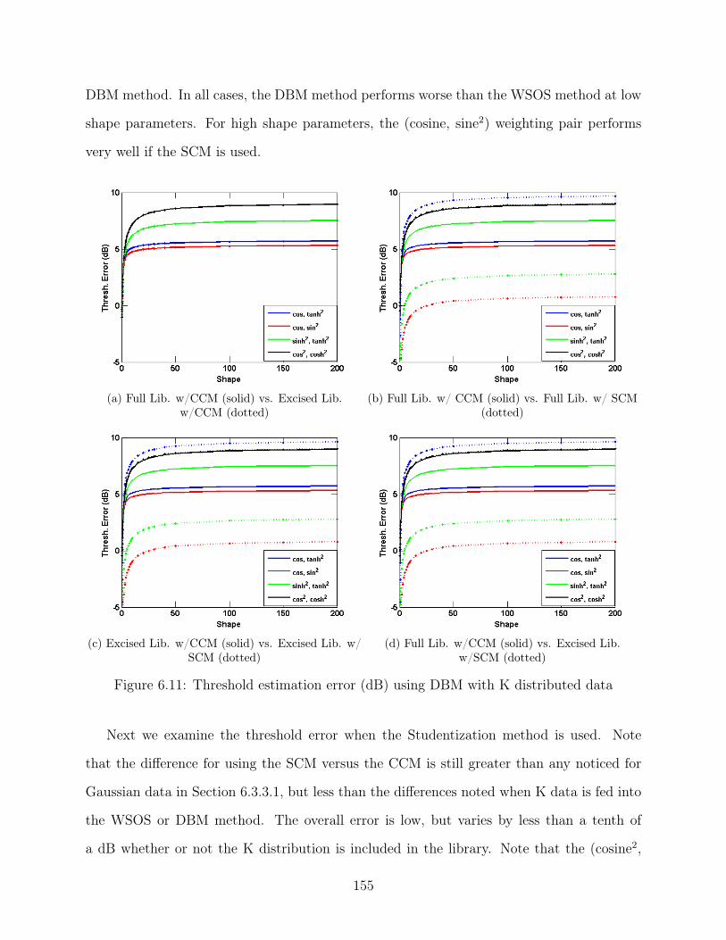
DBM method. In all cases, the DBM method performs worse than the WSOS method at low
shape parameters. For high shape parameters, the (cosine, sine2) weighting pair performs
very well if the SCM is used.
(a) Full Lib. w/CCM (solid) vs. Excised Lib.w/CCM (dotted)
(b) Full Lib. w/ CCM (solid) vs. Full Lib. w/ SCM(dotted)
(c) Excised Lib. w/CCM (solid) vs. Excised Lib. w/SCM (dotted)
(d) Full Lib. w/CCM (solid) vs. Excised Lib.w/SCM (dotted)
Figure 6.11: Threshold estimation error (dB) using DBM with K distributed data
Next we examine the threshold error when the Studentization method is used. Note
that the difference for using the SCM versus the CCM is still greater than any noticed for
Gaussian data in Section 6.3.3.1, but less than the differences noted when K data is fed into
the WSOS or DBM method. The overall error is low, but varies by less than a tenth of
a dB whether or not the K distribution is included in the library. Note that the (cosine2,
155

sine2) weighting pair gives the best results when the covariance matrix is unknown, but the
worst threshold estimation error when the covariance matrix is known. Also, the difference
between the thresholds found using the CCM versus the SCM is on average ≈ 0.6 dB closer
for the (cosine2, sine2) pair than the other two weighting pairs.
Weightings Clairvoyant Cov. Matrix Sample Cov. Matrix
1 2 Full Lib. Excised Lib. Full Lib. Excised Lib. ∆ Clair, SCM
sinh tanh 1.75 1.84 -1.03 -1.01 -2.78
cosh sinh 1.74 1.82 -0.97 -0.96 -2.71
cos2 sine2 2.51 2.56 0.37 0.39 -2.15
Table 6.11: Average Threshold Error (dB) when K distributed data is fed into theStudentized weightings
Figures 6.12a-6.12d examine the impact of using the SCM and excised libraries as com-
pared to the CCM and full libraries when the Studentization method is employed. As was
seen in Table 6.11, there is little difference between using the full or the excised library. How-
ever, when the (cosine2, sine2) pair of weightings are used in conjunction with the SCM, the
resulting average threshold is ≈ 0.5 dB greater than the other two weightings at high shape
parameters, but up to 3.1 dB closer to the true threshold for the lowest of shape parameters.
The former difference translates directly to detection loss, while the latter difference occurs
where the true threshold is 10 dB greater than the threshold needed in Gaussian clutter
of equal power. Therefore the (cosine2, sine2) weighting pair allows for improved perfor-
mance in heavy tailed K distributed clutter at the cost of negligible degradation in detection
loss at lighter tailed clutter, compared to the other weighting pairs. For this reason, the
(cosine2, sine2) weighting pair is the best pair to use with the Studentization method when
K distributed data is encountered.
156

(a) Full Lib. w/CCM (solid) vs. Excised Lib.w/CCM (dotted)
(b) Full Lib. w/ CCM (solid) vs. Full Lib. w/ SCM(dotted)
(c) Excised Lib. w/CCM (solid) vs. Excised Lib. w/SCM (dotted)
(d) Full Lib. w/CCM (solid) vs. Excised Lib.w/SCM (dotted)
Figure 6.12: Threshold estimation error (dB) using Studentized method with K distributeddata
Finally we examine the EOA method. Note that on average, the EOA method produces
worse threshold estimates compared to the Studentization method. Once more, excising the
K distribution from the library makes minimal difference in estimated threshold. However,
the (sine2, sinh2) threshold estimate is only reduced by ≈ 1 dB on average when the SCM
is used.
157

Weightings Clairvoyant Cov. Matrix Sample Cov. Matrix
1 2 Full Lib. Excised Lib. Full Lib. Excised Lib. ∆ Clair, SCM
cos cos2 2.25 2.29 -0.37 -0.35 -2.62
cos2 tanh2 2.10 2.11 -0.73 -0.72 -2.83
sine2 sinh2 5.69 5.69 4.77 4.77 -0.93
Table 6.12: Average Threshold Error (dB) when K distributed data is fed into the EOAweightings
Figures 6.13a-6.13d illustrate the results of Table 6.12 as a function of shape parameter.
Note that while the (sine2, sinh2) weighting pair provides an accurate threshold estimate at
low shape parameter values, it suffers more than a 7 dB loss over the optimal threshold at
high shape parameter values. However, the other weighting pairs will cause a sharp increase
in false alarm rates at low shape parameters.
158

(a) Full Lib. w/CCM (solid) vs. Excised Lib.w/CCM (dotted)
(b) Full Lib. w/ CCM (solid) vs. Full Lib. w/ SCM(dotted)
(c) Excised Lib. w/CCM (solid) vs. Excised Lib. w/SCM (dotted)
(d) Full Lib. w/CCM (solid) vs. Excised Lib.w/SCM (dotted)
Figure 6.13: Threshold estimation error (dB) using EOA method with K distributed data
Overall the WSOS with (cosine, tanh2) and (cosine, sine2) weightings and Studentiza-
tion method with (cosine2, sine2) weightings provide the closest approximation to the true
threshold when K data is present and the SCM is used. It is not recommended to use the
DBM or EOA method when K data is present.
6.3.3.3 Weibull Data
Here we examine the thresholds estimated by the four COSMiC transformation methods
when Weibull distributed data is present. Table 6.13 shows the average threhold estimation
159

error for the WSOS and DBM methods, averaged over shape parameters 1.1 ≤ ν ≤ 2
(note that the value of ν = 2 is equivalent to the Gaussian distribution). It is established
in Section 6.3.1 that the WSOS method tends to select the Weibull distribution. As a
consequence, Table 6.13 shows a large discrepancy in values shown for the full library and
excised library when the true covariance matrix is used. However, the impact of leaving the
Weibull distribution out of the library is heavily dependent on the pair of weightings chosen.
Weightings Clairvoyant Cov. Matrix Sample Cov. Matrix SCM - DBM Weightings ∆ Clair, SCM
1 2 Full Lib. Excised Lib. Full Lib. Excised Lib. Full Lib. Excised Lib. ∆ WSOS ∆ SCM
cos tanh2 1.16 3.44 -0.34 -0.34 6.46 6.37 -1.50 5.30
cos sine2 1.61 2.10 -0.82 -0.44 -2.19 -3.09 -2.44 -3.80
sinh2 tanh2 0.91 2.89 -1.53 -0.71 -0.04 -3.09 -2.45 -0.95
cos2 cosh2 1.03 3.77 -1.83 -0.90 5.92 4.36 -2.86 4.89
Table 6.13: Average Threshold Error (dB) when Weibull distributed data is fed into theWSOS and DBM weightings
Figures 6.14a-6.14d show the results of Table 6.13 for the WSOS transformation method
as a function of shape parameter. It is important to remember that the ideal threshold as
a function of shape parameter is not linear. The threshold at ν = 1.1 is approximately
7.6 dB greater than the threshold of the Gaussian threshold. By examination of Figures
6.14a-6.14d, when the thresholds resulting from the excised library are worse than the full
library when the true covariance matrix is known. However, when the WSOS transformation
method is used with the SCM, the excised library achieves threshold estimates closer to the
true value than the full library over the full range of shape parameters. In addition, the four
weighting pairs under consideration produce closer (i.e. more robust) results than when the
full library is used. If the true covariance matrix could be accurately estimated, the WSOS
technique is capable of giving average threshold results of ≈ ±1 dB over the range of shape
parameters.
160

(a) Full Lib. w/CCM (solid) vs. Excised Lib.w/CCM (dotted)
(b) Full Lib. w/ CCM (solid) vs. Full Lib. w/ SCM(dotted)
(c) Excised Lib. w/CCM (solid) vs. Excised Lib. w/SCM (dotted)
(d) Full Lib. w/CCM (solid) vs. Excised Lib.w/SCM (dotted)
Figure 6.14: Threshold estimation error (dB) using WSOS with Weibull distributed data
Next Figure 6.15a-6.15d shows the corresponding results when the DBM method is used.
It is clear that the WSOS method is superior to the DBM method. Both the use of the SCM
and the excised library prompt large swings in the estimated threshold from the optimum
levels.
161

(a) Full Lib. w/CCM (solid) vs. Excised Lib.w/CCM (dotted)
(b) Full Lib. w/ CCM (solid) vs. Full Lib. w/ SCM(dotted)
(c) Excised Lib. w/CCM (solid) vs. Excised Lib. w/SCM (dotted)
(d) Full Lib. w/CCM (solid) vs. Excised Lib.w/SCM (dotted)
Figure 6.15: Threshold estimation error (dB) using DBM with Weibull distributed data
Table 6.14 then examines the average accuracy of the Studentization transformationmethod. On the surface the Studentization transformation method appears to offer excellentaccuracy that varies little whether or not the excised library or SCM is used, but only whenconsidering the average threshold estimate over the range of shape parameters.
Weightings Clairvoyant Cov. Matrix Sample Cov. Matrix
1 2 Full Lib. Excised Lib. Full Lib. Excised Lib. ∆ Clair, SCM
sinh tanh 1.07 0.73 -1.89 -2.12 -2.96
cosh sinh 1.06 0.74 -1.78 -1.98 -2.84
cos2 sine2 2.00 2.13 -0.55 -0.37 -2.55
Table 6.14: Average Threshold Error (dB) when Weibull distributed data is fed into theStudentized weightings
162

However, Figures 6.16a-6.16d show the accuracy of the Studentization method as a func-
tion of shape parameter. It can be seen from examining the plots in Figures 6.16a-6.16d that
the average values for the excised and when the SCM is used do not convey the behavior
for the different shape parameters. In general, the threshold given is not accurate for the
Studentized transformation method. Only the (cosine, sine2) weighting pair yields adequate
accuracy when the SCM is used.
(a) Full Lib. w/CCM (solid) vs. Excised Lib.w/CCM (dotted)
(b) Full Lib. w/ CCM (solid) vs. Full Lib. w/ SCM(dotted)
(c) Excised Lib. w/CCM (solid) vs. Excised Lib. w/SCM (dotted)
(d) Full Lib. w/CCM (solid) vs. Excised Lib.w/SCM (dotted)
Figure 6.16: Threshold estimation error (dB) using Studentized method with Weibulldistributed data
Table 6.15 examines the last transformation method under discussion, the EOA. From the
163

average values given, only the weighting pair appears to be inappropriate for consideration.
Recall that the EOA for the Weibull distribution was considered for a limited library in
Section 6.3.1.
Weightings Clairvoyant Cov. Matrix Sample Cov. Matrix
1 2 Full Lib. Excised Lib. Full Lib. Excised Lib. ∆ Clair, SCM
cos cos2 1.63 1.27 -1.26 -1.64 -2.89
cos2 tanh2 1.46 1.16 -1.59 -1.98 -3.06
sine2 sinh2 5.28 5.42 4.15 4.25 -1.13
Table 6.15: Average Threshold Error (dB) when Weibull distributed data is fed into theEOA weightings
The results of Table 6.15 are show as a function of shape parameter in Figures 6.17a-6.17d.
The (sine2, sinh2) weighting pair is the only pair that gives adequate threshold estimation
performance at low values of the shape parameter. However, we do not consider the ≈ 7 dB
detection loss when Gaussian data is present to be acceptable.
164

(a) Full Lib. w/CCM (solid) vs. Excised Lib.w/CCM (dotted)
(b) Full Lib. w/ CCM (solid) vs. Full Lib. w/ SCM(dotted)
(c) Excised Lib. w/CCM (solid) vs. Excised Lib. w/SCM (dotted)
(d) Full Lib. w/CCM (solid) vs. Excised Lib.w/SCM (dotted)
Figure 6.17: Threshold estimation error (dB) using EOA method with Weibull distributeddata
Examination of Tables 6.13-6.15 and Figures 6.14a-6.17d suggests that the weighting
pair (cosine, sine2) used in conjunction with the Studentization transformation method is
the only acceptable COSMiC method for setting a threshold in complex Weibull distributed
clutter.
165

6.3.3.4 Pareto Data
Table 6.16 shows the average threshold error for the WSOS and DBM transformation meth-
ods when Pareto data is present. With the exception of the (cosine2, cosh2) weighting pair,
both the WSOS and DBM methods underestimate the true threshold. Therefore, the Pareto
data will cause more false alarms when the WSOS and DBM transformation methods are
used.
Weightings Clairvoyant Cov. Matrix Sample Cov. Matrix SCM - DBM Weightings ∆ Clair, SCM
1 2 Full Lib. Excised Lib. Full Lib. Excised Lib. Full Lib. Excised Lib. ∆ WSOS ∆ SCM
cos tanh2 -1.19 -1.35 -1.87 -2.01 6.97 6.97 -0.68 8.15
cos sine2 -0.44 -1.01 -1.88 -2.12 -1.94 -1.94 -1.45 -1.50
sinh2 tanh2 -0.90 -1.14 -2.09 -2.26 0.09 0.09 -1.18 1.00
cos2 cosh2 -0.30 -0.51 -1.94 -2.25 6.30 6.30 -1.64 6.60
Table 6.16: Average Threshold Error (dB) when Pareto distributed data is fed into theWSOS and DBM weightings
Figures 6.18a-6.18d show the results of Table 6.16 as a function of shape parameter.
Note that when that the difference between the excised library and full library when the
SCM is used is approximately 0.5 dB (at the lowest shape pameter value) to less than a few
hundredths of a dB. The difference between the threshold estimate for the full library with
true clairvoyant covariance matrix and the excised library with the SCM ranges between a
1.95 - 0.5 dB difference (with relation to the increasing shape parameter).
166

(a) Full Lib. w/CCM (solid) vs. Excised Lib.w/CCM (dotted)
(b) Full Lib. w/ CCM (solid) vs. Full Lib. w/ SCM(dotted)
(c) Excised Lib. w/CCM (solid) vs. Excised Lib. w/SCM (dotted)
(d) Full Lib. w/CCM (solid) vs. Excised Lib.w/SCM (dotted)
Figure 6.18: Threshold estimation error (dB) using WSOS with Pareto distributed data
Figures 6.19a-6.19d show the average threshold estimation accuracy when the DBM
method is used with Pareto data. Note that unlike the WSOS method, when the SCM
is used the (cosine, tanh2) and (cosine2, cosh2) weighting pairs produce much different re-
sults compared to the (cosine, sine2) and (sinh2, tanh2) weighting pairs. In particular, the
former are more accurate for low shape parameter values and result in large amounts of
detection loss for high shape parameter values. Meanwhile, the latter result in very low
thresholds for low shape parameter data but accurate thresholds for high shape parameter
data.
167

(a) Full Lib. w/CCM (solid) vs. Excised Lib.w/CCM (dotted)
(b) Full Lib. w/ CCM (solid) vs. Full Lib. w/ SCM(dotted)
(c) Excised Lib. w/CCM (solid) vs. Excised Lib. w/SCM (dotted)
(d) Full Lib. w/CCM (solid) vs. Excised Lib.w/SCM (dotted)
Figure 6.19: Threshold estimation error (dB) using DBM with Pareto distributed data
Next, Table 6.17 shows results that are on average between 1 and 2 dB off of optimal
threshold values when the Studentized transformation method is used. There appears to be
just over a 2 dB difference when the SCM is used, with little difference when the excised
library is used.
168
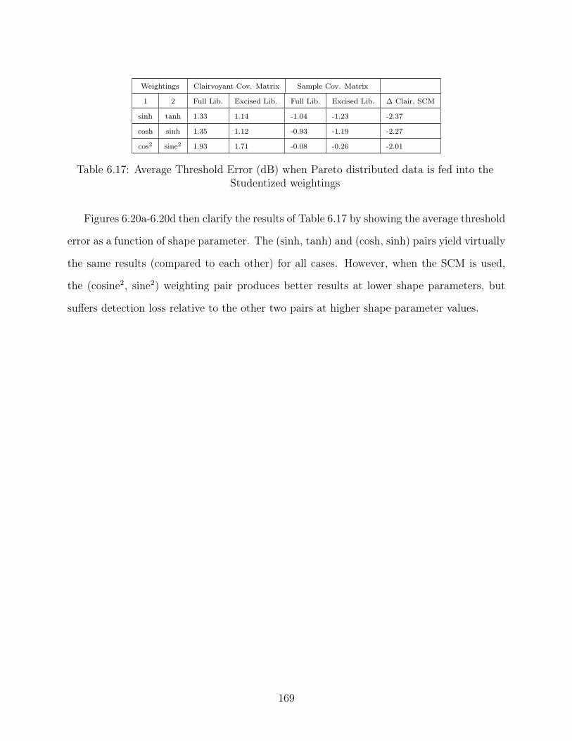
Weightings Clairvoyant Cov. Matrix Sample Cov. Matrix
1 2 Full Lib. Excised Lib. Full Lib. Excised Lib. ∆ Clair, SCM
sinh tanh 1.33 1.14 -1.04 -1.23 -2.37
cosh sinh 1.35 1.12 -0.93 -1.19 -2.27
cos2 sine2 1.93 1.71 -0.08 -0.26 -2.01
Table 6.17: Average Threshold Error (dB) when Pareto distributed data is fed into theStudentized weightings
Figures 6.20a-6.20d then clarify the results of Table 6.17 by showing the average threshold
error as a function of shape parameter. The (sinh, tanh) and (cosh, sinh) pairs yield virtually
the same results (compared to each other) for all cases. However, when the SCM is used,
the (cosine2, sine2) weighting pair produces better results at lower shape parameters, but
suffers detection loss relative to the other two pairs at higher shape parameter values.
169
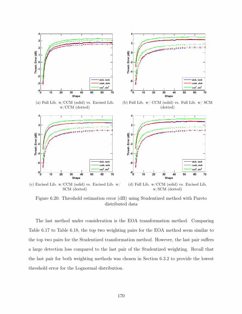
(a) Full Lib. w/CCM (solid) vs. Excised Lib.w/CCM (dotted)
(b) Full Lib. w/ CCM (solid) vs. Full Lib. w/ SCM(dotted)
(c) Excised Lib. w/CCM (solid) vs. Excised Lib. w/SCM (dotted)
(d) Full Lib. w/CCM (solid) vs. Excised Lib.w/SCM (dotted)
Figure 6.20: Threshold estimation error (dB) using Studentized method with Paretodistributed data
The last method under consideration is the EOA transformation method. Comparing
Table 6.17 to Table 6.18, the top two weighting pairs for the EOA method seem similar to
the top two pairs for the Studentized transformation method. However, the last pair suffers
a large detection loss compared to the last pair of the Studentized weighting. Recall that
the last pair for both weighting methods was chosen in Section 6.3.2 to provide the lowest
threshold error for the Lognormal distribution.
170

Weightings Clairvoyant Cov. Matrix Sample Cov. Matrix
1 2 Full Lib. Excised Lib. Full Lib. Excised Lib. ∆ Clair, SCM
cos cos2 1.74 1.42 -0.65 -0.82 -2.39
cos2 tanh2 1.69 1.35 -0.78 -1.08 -2.47
sine2 sinh2 5.55 5.60 4.69 4.69 -0.86
Table 6.18: Average Threshold Error (dB) when Pareto distributed data is fed into theEOA weightings
The accuracy of the threshold estimation shown in Table 6.18 is given as a function
of shape parameter in Figures 6.21a-6.21d. The top two weightings result in a compara-
ble accuracy to the top two weightings for the Studentized method. However, the (sine2,
sinh2) weighting pair results in a very large detection loss for high shape parameter values.
Therefore, the (sine2, sinh2) weighting pair should not be used in conjunction with the EOA
method.
171

(a) Full Lib. w/CCM (solid) vs. Excised Lib.w/CCM (dotted)
(b) Full Lib. w/ CCM (solid) vs. Full Lib. w/ SCM(dotted)
(c) Excised Lib. w/CCM (solid) vs. Excised Lib. w/SCM (dotted)
(d) Full Lib. w/CCM (solid) vs. Excised Lib.w/SCM (dotted)
Figure 6.21: Threshold estimation error (dB) using EOA method with Pareto distributeddata
In general, the Studentized method provides the most accurate threshold estimates, with
(cosine2, sine2) offering best low shape parameter results and the (sinh, tanh) and (cosh,
sinh) weighting pairs offering the best high shape parameter results. The top two weighting
pairs for the EOA transformation method provide comparable results to the Studentized
method.
172

6.3.3.5 Lognormal Data
Note that for the parameters under consideration, the Lognormal distribution requires athreshold 10 dB greater than the threshold needed for the same probability of false alarmin complex Gaussian noise. Table 6.19 shows the average estimated threshold error forLognormal clutter when the WSOS and DBM methods are used to estimate the threshold.When the DBM method is used, both the (cosine, tanh2) and (cosine2, cosh2) weightingcombinations yield very accurate threshold estimates.
Weightings Clairvoyant Cov. Matrix Sample Cov. Matrix SCM - DBM Weightings ∆ Clair, SCM
1 2 Full Lib. Excised Lib. Full Lib. Excised Lib. Full Lib. Excised Lib. ∆ WSOS ∆ SCM
cos tanh2 -5.58 -5.62 -6.42 -6.43 -0.50 -0.50 -0.84 5.09
cos sine2 -3.36 -3.57 -5.79 -5.92 -9.30 -9.30 -2.43 -5.94
sinh2 tanh2 -4.82 -4.88 -6.51 -6.52 -7.04 -7.04 -1.68 -2.22
cos2 cosh2 -5.04 -5.12 -5.64 -5.81 -0.88 -0.88 -0.61 4.15
Table 6.19: Average Threshold Error (dB) when Lognormal distributed data is fed into theWSOS and DBM weightings
Next the performance of the Studentized transformation method is examined in Table
6.20. Despite the difference in performance between the WSOS and Studentized methods
when the true covariance matrix is used, the Studentized method has an average threshold
error equal to or better than the WSOS method. However, the top two DBM weighting pairs
outperform all three of the Studentized pairs.
Weightings Clairvoyant Cov. Matrix Sample Cov. Matrix
1 2 Full Lib. Excised Lib. Full Lib. Excised Lib. ∆ Clair, SCM
sinh tanh -2.58 -2.59 -6.00 -6.01 -3.42
cosh sinh -2.64 -2.65 -6.15 -6.17 -3.51
cos2 sine2 -1.90 -1.90 -4.15 -4.15 -2.25
Table 6.20: Average Threshold Error (dB) when Lognormal distributed data is fed into theStudentized weightings
Finally, Table 6.21 shows the average threshold error when the EOA transformation
method is applied to Lognormal data. In this case, the (sine2, sinh2) pairing is the best
choice whether or not the covariance matrix is known.
173

Weightings Clairvoyant Cov. Matrix Sample Cov. Matrix
1 2 Full Lib. Excised Lib. Full Lib. Excised Lib. ∆ Clair, SCM
cos cos2 -2.02 -2.10 -4.97 -5.01 -2.95
cos2 tanh2 -2.35 -2.41 -5.66 -5.74 -3.31
sine2 sinh2 -0.72 -0.80 -1.52 -1.58 -0.80
Table 6.21: Average Threshold Error (dB) when Lognormal distributed data is fed into theEOA weightings
Overall, when Lognormal data is present, the EOA transformation method and weighting
pair (sine2, sinh2) offers the best results when the covariance matrix is known, but also the
second best accuracy when the sample covariance matrix is used. However, if the sample
covariance matrix is used the (cosine2, cosh2) and (cosine, tanh2) weightings work best when
transformed via the DBM method.
6.4 Evaluating Triplets of Weightings in COSMiC
Section 6.3 considered the use of pairs of weighting functions in conjunction with four trans-
formation methods to identify the distribution and threshold associated with various distri-
butions. This section considers the extension from pairs of weighting functions to triplets of
weighting functions. In other words, does the addition of a weighting function provide di-
versity and improve the results established in Section 6.3? Experimentation showed that the
underlying endpoint space is symmetric. Therefore, with 10 candidate weighting functions,
only 120 combinations of triplets of weightings needed to be considered (versus the 45 pairs
of weightings considered).
Section 6.4.1 examines the problem of distribution identification, while Sections 6.4.2-
6.4.3.5 examine the utility of using triplets of weightings to estimate the threshold in the
presence of the distributions under test.
174

6.4.1 Distribution Identification with Triplets of Weightings
The distribution identification accuracy of the proposed transformation methods (excepting
the DBM method) when three weightings are used to form the endpoint is shown in Tables
6.22-6.24. Comparing Tables 6.22-6.24 to Tables 6.1-6.3 it appears that the use of triplets of
weightings actually slightly degrades the distribution identification capabilities of all three
transformation methods when compared to using pairs of weightings.
Weightings Percentage Chosen
True Dist. 1 2 3 Gaussian K Weibull Pareto Lognormal Gamma Mod.
Gaussian sine2 cosh cosh2 49.1 5.0 43.3 2.5 0.0 0.1
K sinh2 tanh tanh2 0.1 3.1 96.6 0.0 0.0 0.2
Weibull sine sine2 cosh 12.7 18.7 64.9 2.0 0.1 1.6
Pareto cos cos2 sine 24.6 8.5 38.9 24.2 1.3 2.5
Lognormal cos cos2 sine 12.6 8.3 27.6 34.5 6.7 10.3
Table 6.22: Distribution identification percentages of top WSOS COSMiC weightingtriplets
Weightings Percentage Chosen
True Dist. 1 2 3 Gaussian K Weibull Pareto Lognormal Gamma Mod.
Gaussian sinh sinh2 tanh 45.8 3.5 35.3 12.3 1.3 1.7
K cos cos2 sine 22.2 22.1 41.4 8.6 2.1 3.7
Weibull sine2 cosh cosh2 24.6 13.8 47.6 8.4 1.9 3.6
Pareto cos2 sine sine2 26.3 11.8 42.5 11.8 3.0 4.6
Lognormal cos2 sine sine2 5.0 41.9 38.5 4.9 3.4 6.3
Table 6.23: Distribution identification percentages of top Studentized COSMiC weightingtriplets
Weightings Percentage Chosen
True Dist. 1 2 3 Gaussian K Weibull Pareto Lognormal Gamma Mod.
Gaussian sinh2 tanh tanh2 42.9 2.8 39.9 12.3 0.9 1.2
K sinh2 tanh tanh2 21.3 18.6 41.5 11.4 3.0 4.2
Weibull cosh cosh2 sinh 16.9 9.4 51.9 13.1 4.5 4.1
Pareto cos2 sine sine2 20.0 7.2 38.4 22.8 7.2 4.4
Lognormal cos cos2 sine 5.6 30.7 31.7 10.9 12.8 8.3
Table 6.24: Distribution identification percentages of top EOA COSMiC weighting triplets
175

The distribution identification performance as a function of shape paramter is shown for
the two triplets of weightings with the highest identification accuracy when K, Weibull, and
Pareto distributed data is present is shown in Figures 6.22a-6.24c. In light of the decreased
performance of the triplets when compared to using pairs of weightings, the results are
presented without further comment.
(a) (sinh2, tanh, tanh2) (solid) vs. (cosh2, sinh,sinh2) (dotted)
(b) (cos, cos2, sine) (solid) vs. (cos, cos2, sine2)(dotted)
(c) (sinh2, tanh, tanh2) (solid) vs. (cosh2, sinh,sinh2) (dotted)
Figure 6.22: COSMiC distribution identification vs. shape parameter for Weibulldistributed data for top triplets
176

(a) (sine, sine2, cosh) vs. (sine, sine2, cosh2) (solid)(dotted)
(b) (sine2, cosh, cosh2) (solid) vs. (sine2, cosh, sinh)(dotted)
(c) (cosh, cosh2, sinh) (solid) vs. (cosh, cosh2, sinh2)(dotted)
Figure 6.23: COSMiC distribution identification vs. shape parameter for Weibulldistributed data for top triplets
177

(a) (cos, cos2, sine) (solid) vs. (cos, cos2, sine2)(dotted)
(b) (cos2, sine, sine2) (solid) vs. (cos2, sine, cosh)(dotted)
(c) (cos2, sine, sine2) (solid) vs. (cos2, sine, cosh)(dotted)
Figure 6.24: COSMiC distribution identification v. shape parameter for Pareto distributeddata for top triplets
6.4.2 Threshold Estimation - Identifying Top Triplet Weightings
The most accurate (averaged over all values of shape parameter) triplet of weighting func-
tions is reported for each distribution/transformation combination in the same manner as
was shown in Section 6.3.2. Despite the degradation noted in distribution identification, com-
paring Tables 6.4 and 6.5 to Tables 6.25 and 6.26, respectively, shows that for the WSOS
and Studentization transformation methods the use of triplets of weightings provides a slight
improvement in threshold estimation accuracy when compared to using pairs of weightings.
178

However, comparing Tables 6.6 and 6.27, only the Lognormal distribution has an improved
threshold estimate when the EOA transformation method is used with triplets of weight-
ings. In addition, the top pairs of weightings are present in one or more of the top triplets of
weightings for each method. Therefore, addition of the third weighting function only offers
a slight improvement, if any, over the pair of weightings. This result implys that there is
little new information gained by adding the third endpoint.
Weightings Gaussian K Weibull Pareto Lognormal
1 2 3 Rank Error Rank Error Rank Error Rank Error Rank Error
cos sinh2 tanh2 1 0.76 dB 2 4.94 dB 33 1.14 dB 114 -1.17 dB 92 -5.46 dB
cos sine2 tanh2 26 1.04 dB 1 4.40 dB 101 1.56 dB 26 -0.54 dB 12 -3.41 dB
cos2 cosh cosh2 88 1.35 dB 90 6.52 dB 1 1.01 dB 54 -0.70 dB 86 -5.30 dB
cos2 sine2 tanh2 107 1.73 dB 46 6.29 dB 96 1.48 dB 1 0.06 dB 11 -3.25 dB
sine sine2 tanh 119 4.68 dB 119 6.67 dB 119 3.22 dB 119 3.02 dB 1 -1.40 dB
Table 6.25: Summary of top WSOS weighting triplets
Weightings Gaussian K Weibull Pareto Lognormal
1 2 3 Rank Error Rank Error Rank Error Rank Error Rank Error
cos sinh tanh2 1 2.77 dB 1 1.64 dB 1 0.98 dB 1 1.27 dB 119 -2.61 dB
cos sinh tanh2 1 2.77 dB 1 1.64 dB 1 0.98 dB 1 1.27 dB 119 -2.61 dB
cos sinh tanh2 1 2.77 dB 1 1.64 dB 1 0.98 dB 1 1.27 dB 119 -2.61 dB
cos sinh tanh2 1 2.77 dB 1 1.64 dB 1 0.98 dB 1 1.27 dB 119 -2.61 dB
cos2 cosh2 sinh2 114 3.54 dB 116 2.37 dB 116 1.86 dB 112 1.91 dB 1 -1.86 dB
Table 6.26: Summary of top studentized weighting triplets
Weightings Gaussian K Weibull Pareto Lognormal
1 2 3 Rank Error Rank Error Rank Error Rank Error Rank Error
cos cos2 tanh2 1 3.28 dB 1 2.28 dB 1 1.74 dB 1 1.81 dB 70 -1.90 dB
cos cos2 tanh2 1 3.28 dB 1 2.28 dB 1 1.74 dB 1 1.81 dB 70 -1.90 dB
cos cos2 tanh2 1 3.28 dB 1 2.28 dB 1 1.74 dB 1 1.81 dB 70 -1.90 dB
cos cos2 tanh2 1 3.28 dB 1 2.28 dB 1 1.74 dB 1 1.81 dB 70 -1.90 dB
sine2 sinh2 tanh2 114 7.94 dB 115 5.70 dB 115 5.32 dB 114 5.57 dB 1 -0.67 dB
Table 6.27: Summary of top extended Ozturk weighting triplets
179

6.4.3 Threshold Estimation with Triplets of Weightings - Evaluat-
ing Robustness of COSMiC Methods
Sections 6.4.3.1-6.4.3.5 follow in the footsteps of Sections 6.3.3.1-6.3.3.5 by showing the accu-
racy of the threshold estimate produced by the pairing of the various weighting triplets/trans-
formation methods when the test data is distributed according to the candidate distributions.
The numerical results are reported in the tables and figures, while the analysis is primarily
concerned with the comparison to the corresponding scenario when a pair of weightings is
used. In other words, for each case what is the benefit of using the third weighting function?
6.4.3.1 Gaussian Data
Compared to the results in Section 6.3.3.1, when Gaussian data is present there is little to
no increase in average threshold estimate error offered by using the third weightings.
Weightings Clairvoyant Cov. Matrix Sample Cov. Matrix SCM - DBM Weightings ∆ Clair, SCM
1 2 3 Full Lib. Excised Lib. Full Lib. Excised Lib. Full Lib. Excised Lib. ∆ WSOS ∆ DBM
cos sinh2 tanh2 0.83 0.83 0.35 0.36 9.82 9.82 -0.47 8.99
cos sine2 tanh2 1.02 1.02 0.34 0.34 0.92 0.92 -0.68 -0.10
cos2 cosh cosh2 1.69 1.70 0.55 0.56 0.00 0.02 -1.14 -1.68
cos2 sine2 tanh2 1.40 1.40 0.33 0.33 7.50 7.50 -1.07 6.10
sine sine2 tanh 4.72 4.72 0.64 0.64 0.00 0.92 -4.08 -4.72
Table 6.28: Average Threshold Error (dB) when Gaussian distributed data is fed into theWSOS and DBM weightings
Weightings Clairvoyant Cov. Matrix Sample Cov. Matrix
1 2 3 Full Lib. Excised Lib. Full Lib. Excised Lib. ∆ Clair, SCM
cos sinh tanh2 2.86 2.86 1.52 1.52 -1.34
cos2 cosh2 sinh2 3.37 3.44 2.02 2.15 -1.35
Table 6.29: Average Threshold Error (dB) when Gaussian distributed data is fed into theStudentized weightings
180

Weightings Clairvoyant Cov. Matrix Sample Cov. Matrix
1 2 3 Full Lib. Excised Lib. Full Lib. Excised Lib. ∆ Clair, SCM
cos cos2 tanh2 3.19 3.22 1.70 1.77 -1.49
sine2 sinh2 tanh2 7.96 7.97 7.29 7.29 -0.68
Table 6.30: Average Threshold Error (dB) when Gaussian distributed data is fed into theEOA weightings
6.4.3.2 K Data
Comparing Tables 6.10 and 6.31 the weighting pairs (cosine, tanh2) and (sinh2, tanh2) were
combined into the triplet (cosine, sinh2, tanh2). The resultant combination yields decreased
performance when the SCM is used for the WSOS transformation method due to the inclusion
of the sinh2 weighting, and greatly decreased performance of the DBM method due to the
inclusion of the cosine weighting. This example shows that the disadvantages of different
weightings can be combined to form a triplet that performs worse than the separate pairs of
weightings. Therefore, rather than introducing diversity in the form additional endpoints to
a single set of weightings, it may be more effective to incorporate multiple pairs of weightings.
This concept should be explored in future work.
Weightings Clairvoyant Cov. Matrix Sample Cov. Matrix SCM - DBM Weightings ∆ Clair, SCM
1 2 3 Full Lib. Excised Lib. Full Lib. Excised Lib. Full Lib. Excised Lib. ∆ WSOS ∆ DBM
cos sinh2 tanh2 4.96 4.96 -0.89 -0.38 6.74 6.68 -5.85 1.78
cos sine2 tanh2 4.42 4.42 -0.93 -0.60 -1.91 -1.91 -5.35 -6.33
cos2 cosh cosh2 6.30 6.31 -0.99 -0.84 -2.40 -2.40 -7.29 -8.70
cos2 sine2 tanh2 6.52 6.52 -1.19 -1.04 4.74 4.74 -7.71 -1.79
sine sine2 tanh 6.67 6.68 -0.95 -0.79 -2.78 -2.78 -7.62 -9.45
Table 6.31: Average Threshold Error (dB) when K distributed data is fed into the WSOSand DBM weightings
181

(a) Full Lib. w/CCM (solid) vs. Excised Lib.w/CCM (dotted)
(b) Full Lib. w/ CCM (solid) vs. Full Lib. w/ SCM(dotted)
(c) Excised Lib. w/CCM (solid) vs. Excised Lib. w/SCM (dotted)
(d) Full Lib. w/CCM (solid) vs. Excised Lib.w/SCM (dotted)
Figure 6.25: Threshold estimation error (dB) using WSOS with K distributed data
182

(a) Full Lib. w/CCM (solid) vs. Excised Lib.w/CCM (dotted)
(b) Full Lib. w/ CCM (solid) vs. Full Lib. w/ SCM(dotted)
(c) Excised Lib. w/CCM (solid) vs. Excised Lib. w/SCM (dotted)
(d) Full Lib. w/CCM (solid) vs. Excised Lib.w/SCM (dotted)
Figure 6.26: Threshold estimation error (dB) using DBM with K distributed data
For the Studentized method, the (cos2, cosh2, sinh2) triplet provides a quarter of a decibel
of improvement over the best weighting pair when the SCM is used. However, at the lowest
shape parameter, if the SCM is used both the full and excised libraries produce a threshold
≈ 0.5 dB lower than that of the best weighting pair. Therefore, in general the weighting
pairs are better than the triplets of weightings in this case.
183

Weightings Clairvoyant Cov. Matrix Sample Cov. Matrix
1 2 3 Full Lib. Excised Lib. Full Lib. Excised Lib. ∆ Clair, SCM
cos sinh tanh2 1.67 1.77 -1.05 -0.99 -2.72
cos2 cosh2 sinh2 2.41 2.50 0.07 0.11 -2.34
Table 6.32: Average Threshold Error (dB) when K distributed data is fed into theStudentized weightings
(a) Full Lib. w/CCM (solid) vs. Excised Lib.w/CCM (dotted)
(b) Full Lib. w/ CCM (solid) vs. Full Lib. w/ SCM(dotted)
(c) Excised Lib. w/CCM (solid) vs. Excised Lib. w/SCM (dotted)
(d) Full Lib. w/CCM (solid) vs. Excised Lib.w/SCM (dotted)
Figure 6.27: Threshold estimation error (dB) using Studentized method with K distributeddata
The EOA method produces similar results for the top pairs of weightings and the top
triplets of weightings. The results for the (cosine, cosine2, tanh2) triplet yields an average
184

threshold of ≈ 0.1 dB more than the average threshold for the (cosine, cosine2) weighting
pair for all values of the shape parameter.
Weightings Clairvoyant Cov. Matrix Sample Cov. Matrix
1 2 3 Full Lib. Excised Lib. Full Lib. Excised Lib. ∆ Clair, SCM
cos cos2 tanh2 1.67 1.77 -1.05 -0.99 -2.72
sine2 sinh2 tanh2 2.41 2.50 0.07 0.11 -2.34
Table 6.33: Average Threshold Error (dB) when K distributed data is fed into the EOAweightings
(a) Full Lib. w/CCM (solid) vs. Excised Lib.w/CCM (dotted)
(b) Full Lib. w/ CCM (solid) vs. Full Lib. w/ SCM(dotted)
(c) Excised Lib. w/CCM (solid) vs. Excised Lib. w/SCM (dotted)
(d) Full Lib. w/CCM (solid) vs. Excised Lib.w/SCM (dotted)
Figure 6.28: Threshold estimation error (dB) using EOA method with K distributed data
185

6.4.3.3 Weibull Data
Upon examination of the average errors in threshold estimate given in Table 6.34, it appears
that there is no advantage to using triplets of weighting functions rather than pairs of
weighting functions when the WSOS transformation method is employed and Weibull data
is present.
Weightings Clairvoyant Cov. Matrix Sample Cov. Matrix SCM - DBM Weightings ∆ Clair, SCM
1 2 3 Full Lib. Excised Lib. Full Lib. Excised Lib. Full Lib. Excised Lib. ∆ WSOS ∆ DBM
cos sinh2 tanh2 1.13 3.63 -0.47 -0.45 6.25 6.02 -1.60 5.12
cos sine2 tanh2 1.55 2.16 -0.83 -0.44 -2.22 -3.09 -2.39 -3.77
cos2 cosh cosh2 1.47 1.86 -1.35 -1.32 -2.91 -2.97 -2.82 -4.38
cos2 sine2 tanh2 0.98 3.90 -1.51 -0.87 4.37 4.77 -2.50 3.39
sine sine2 tanh 3.21 1.90 -1.19 -1.30 -3.09 -3.09 -4.40 -6.29
Table 6.34: Average Threshold Error (dB) when Weibull distributed data is fed into theWSOS and DBM weightings
However, when the threshold error is shown as a function of shape parameter, it is
apparent that Table 6.34 does not tell the entire story. Comparing Figures 6.29a-6.29d with
Figures 6.14a-6.14d, the use of weighting triplets appears to mitigate the wide swings in
threshold estimation error (as a function of shape parameter) that arise when the SCM is
used with the WSOS transformation method. In particular, the triplets of weightings tend
not to overestimate the threshold. However, the underestimation of the threshold error
will cause an increase in false alarms. It should be noted that the false alarms resulting
from this increase will be less than the false alarms the detector would experience if the
threshold for Gaussian data is used when Weibull clutter is present (i.e. the traditional
radar assumption). Despite the improvement in performance over using pairs of weighting
functions, the top triplets for the WSOS transformation method still provide worse threshold
estimates than the top pair for the Studentization method when Weibull data is present.
186

(a) Full Lib. w/CCM vs. Excised Lib. w/CCM(dotted) (b) Full Lib. w/ CCM vs. Full Lib. w/ SCM (dotted)
(c) Excised Lib. w/CCM vs. Excised Lib. w/ SCM(dotted)
(d) Full Lib. w/CCM vs. Excised Lib. w/SCM(dotted)
Figure 6.29: Threshold estimation error (dB) using WSOS with Weibull distributed data
187
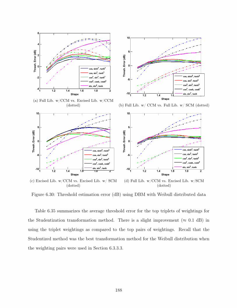
(a) Full Lib. w/CCM vs. Excised Lib. w/CCM(dotted) (b) Full Lib. w/ CCM vs. Full Lib. w/ SCM (dotted)
(c) Excised Lib. w/CCM vs. Excised Lib. w/ SCM(dotted)
(d) Full Lib. w/CCM vs. Excised Lib. w/SCM(dotted)
Figure 6.30: Threshold estimation error (dB) using DBM with Weibull distributed data
Table 6.35 summarizes the average threshold error for the top triplets of weightings for
the Studentization transformation method. There is a slight improvement (≈ 0.1 dB) in
using the triplet weightings as compared to the top pairs of weightings. Recall that the
Studentized method was the best transformation method for the Weibull distribution when
the weighting pairs were used in Section 6.3.3.3.
188

Weightings Clairvoyant Cov. Matrix Sample Cov. Matrix
1 2 3 Full Lib. Excised Lib. Full Lib. Excised Lib. ∆ Clair, SCM
cos sinh tanh2 0.97 0.87 -1.86 -1.95 -2.83
cos2 cosh2 sinh2 1.83 1.36 -0.79 -1.36 -2.62
Table 6.35: Average Threshold Error (dB) when Weibull distributed data is fed into theStudentized weightings
However, examination of Figures 6.31a-6.31d shows that the impact of the sample co-
variance matrix overwhelms the slight advantage gained through use of the extra weighting.
Therefore, it does not appear that the Studentized method benefits from the use of three
weighting functions as compared to two.
189

(a) Full Lib. w/CCM vs. Excised Lib. w/CCM(dotted) (b) Full Lib. w/ CCM vs. Full Lib. w/ SCM (dotted)
(c) Excised Lib. w/CCM vs. Excised Lib. w/ SCM(dotted)
(d) Full Lib. w/CCM vs. Excised Lib. w/SCM(dotted)
Figure 6.31: Threshold estimation error (dB) using Studentized method with Weibulldistributed data
Examining Tables 6.15 and 6.36 shows that when the CCM is used, there is a slight
improvement (≈ 0.07 dB) when the (cos, cos2, tanh2) triplet of weightings is used compared
to when the weighting pair (cos, cos2) is employed. However, this slight improvement comes
at the cost of a performance degradation when compared to the estimate given by the
weighting pair (cos2, tanh2). The top weighting triplet does perform better than either pair
when the SCM is used, but the average threshold error is only reduced by < 0.1 dB.
190

Weightings Clairvoyant Cov. Matrix Sample Cov. Matrix
1 2 3 Full Lib. Excised Lib. Full Lib. Excised Lib. ∆ Clair, SCM
cos cos2 tanh2 1.70 1.34 -1.17 -1.59 -2.88
sine2 sinh2 tanh2 5.31 5.49 4.20 4.39 -1.12
Table 6.36: Average Threshold Error (dB) when Weibull distributed data is fed into theEOA weightings
Figures 6.32a-6.32d then illustrate the results of Table 6.36 as a function of shape pa-
rameter. Once more, comparing Figures 6.32a-6.32d to Figures 6.17a-6.17d there is no real
improvement in performance given by adding an extra weighting function.
191

(a) Full Lib. w/CCM vs. Excised Lib. w/CCM(dotted) (b) Full Lib. w/ CCM vs. Full Lib. w/ SCM (dotted)
(c) Excised Lib. w/CCM vs. Excised Lib. w/ SCM(dotted)
(d) Full Lib. w/CCM vs. Excised Lib. w/SCM(dotted)
Figure 6.32: Threshold estimation error (dB) using EOA method with Weibull distributeddata
In general, if Weibull data is present the addition of the extra weighting function does
not greatly improve the threshold estimation accuracy if the covariance matrix is known.
For certain transformation methods (e.g. the EOA) the estimation accuracy improves by a
small amount for select situations. However, this marginal improvement does not necessarily
justify the increased complexity or computational cost caused by the additional weighting
function.
On the other hand, if the covariance matrix is not known, there is a significant advantage
192

to using the triplets of weightings with the WSOS transformation method. Unfortunately,
this added advantage does not result in superior average threshold estimates when compared
to the (cosine, sine2) weighting pair transformed via the Studentization method. Therefore,
it is not necessary to use triplets of weighting functions when Weibull data is present.
6.4.3.4 Pareto Data
It is apparent from comparing Tables 6.37 and 6.16 that the addition of the cosh weighting
function to the weighting pair (cosine2, cosh2) leads to a small improvement (up to 0.3 dB
depending on the scenario) in the threshold estimates given when the WSOS transformation
method is used. However the DBM performance changes from an average detection loss of 6.3
dB to an average threshold estimate error of −2.84 dB (i.e. an underestimate). Therefore,
the DBM method used with a pair of weighting functions causes an average detection loss,
but when a triplet of weightings are employed the loss becomes an average increase in the
probability of false alarm.
Weightings Clairvoyant Cov. Matrix Sample Cov. Matrix SCM - DBM Weightings ∆ Clair, SCM
1 2 3 Full Lib. Excised Lib. Full Lib. Excised Lib. Full Lib. Excised Lib. ∆ WSOS ∆ DBM
cos sinh2 tanh2 -1.18 -1.32 -1.95 -2.07 6.95 6.95 -0.76 8.14
cos sine2 tanh2 -0.53 -1.05 -1.90 -2.13 -1.94 -1.94 -1.36 -1.40
cos2 cosh cosh2 0.07 -0.48 -1.61 -2.01 -2.84 -2.84 -1.68 -2.90
cos2 sine2 tanh2 -0.70 -0.88 -1.91 -2.21 4.65 4.65 -1.21 5.35
sine sine2 tanh 3.04 2.60 -1.58 -1.93 -2.86 -2.86 -4.62 -5.89
Table 6.37: Average Threshold Error (dB) when Pareto distributed data is fed into theWSOS and DBM weightings
Comparing Figures 6.33a-6.33d to Figures 6.18a-6.18d, there is little change in behaviour
of the average threshold estimate as a function of shape parameter between the top triplets
of weightings and the top pairs of weightings when the WSOS transformation method is
used.
193

(a) Full Lib. w/CCM vs. Excised Lib. w/CCM(dotted) (b) Full Lib. w/ CCM vs. Full Lib. w/ SCM (dotted)
(c) Excised Lib. w/CCM vs. Excised Lib. w/ SCM(dotted)
(d) Full Lib. w/CCM vs. Excised Lib. w/SCM(dotted)
Figure 6.33: Threshold estimation error (dB) using WSOS with Pareto distributed data
194

(a) Full Lib. w/CCM vs. Excised Lib. w/CCM(dotted) (b) Full Lib. w/ CCM vs. Full Lib. w/ SCM (dotted)
(c) Excised Lib. w/CCM vs. Excised Lib. w/ SCM(dotted)
(d) Full Lib. w/CCM vs. Excised Lib. w/SCM(dotted)
Figure 6.34: Threshold estimation error (dB) using DBM with Pareto distributed data
Table 6.38 shows the average threshold error for the top triplets of weightings when
the Studentization transformation method is used. From comparing Table 6.38 to Table
6.17, note that the top triplet weightings are not formed from "merging" the top pairs of
weightings. However, the final performance is still very close.
195

Weightings Clairvoyant Cov. Matrix Sample Cov. Matrix
1 2 3 Full Lib. Excised Lib. Full Lib. Excised Lib. ∆ Clair, SCM
cos sinh tanh2 1.27 1.07 -1.01 -1.24 -2.28
cos2 cosh2 sinh2 1.90 1.71 -0.28 -0.37 -2.18
Table 6.38: Average Threshold Error (dB) when Pareto distributed data is fed into theStudentized weightings
Comparing Figures 6.35a-6.35d to Figures 6.20a-6.20d, the average threshold error as a
function of shape parameter when the triplets of weightings are used in conjunction with the
Studentization method is very close to the performance when the top pairs of weightings are
used. However, there is no real improvement to make up for the increased complexity added
by the use of the extra weighting function.
196

(a) Full Lib. w/CCM vs. Excised Lib. w/CCM(dotted) (b) Full Lib. w/ CCM vs. Full Lib. w/ SCM (dotted)
(c) Excised Lib. w/CCM vs. Excised Lib. w/ SCM(dotted)
(d) Full Lib. w/CCM vs. Excised Lib. w/SCM(dotted)
Figure 6.35: Threshold estimation error (dB) using Studentized method with Paretodistributed data
In contrast to the Studentization method, comparing Tables 6.39 and 6.18 shows that the
top two triplets of weighting functions for the EOA transformation method are combinations
of the top three pairs of weighting functions. However, the merging of the top pairs into
triplets of weighting functions actually slightly degrades the average threshold estimate.
197

Weightings Clairvoyant Cov. Matrix Sample Cov. Matrix
1 2 3 Full Lib. Excised Lib. Full Lib. Excised Lib. ∆ Clair, SCM
cos cos2 tanh2 1.81 1.49 -0.58 -0.76 -2.38
sine2 sinh2 tanh2 5.58 5.62 4.72 4.71 -0.86
Table 6.39: Average Threshold Error (dB) when Pareto distributed data is fed into theEOA weightings
Figures 6.36a-6.36d show the average threshold error for the top triplets of weighting
functions used in conjunction with the EOA transformation method as a function of shape
parameter when Pareto distributed data is present. Compared to Figures 6.21a-6.21d, the
error yielded by the triplets is similar, if slightly greater.
198

(a) Full Lib. w/CCM vs. Excised Lib. w/CCM(dotted) (b) Full Lib. w/ CCM vs. Full Lib. w/ SCM (dotted)
(c) Excised Lib. w/CCM vs. Excised Lib. w/ SCM(dotted)
(d) Full Lib. w/CCM vs. Excised Lib. w/SCM(dotted)
Figure 6.36: Threshold estimation error (dB) using EOA method with Pareto distributeddata
Using triplets of weightings instead of pairs of weightings resulted in a slight increase
in threshold estimation accuracy when the WSOS transformation method was employed.
However, the top pair of weighting functions combined with the Studentization method still
gives the best threshold estimate for Pareto data when compared to all other transformation
methods and weighting function combinations. Examination of the Studentization method
shows that there are not necessarily superior weighting functions, as the top triplets were
different than the top pairs. However, the top triplets of the EOA method were combinations
199

of the top three pairs of weightings. Therefore, more work is needed to isolate the effects of
the individual weightings.
6.4.3.5 Lognormal Data
Table 6.40 shows the average threshold error in the estimates for the Lognormal distribution
when the WSOS and DBM transformation methods are used and the endpoints are generated
from triplets of weighting functions. Comparing the results to Table 6.19, most of the average
threshold estimates given by the triplets yield little improvement to actual degradation
relation to the top weighting pairs. However, the (sine, sine2, tanh) triplet provides an
excellent estimate when the true covariance matrix is known.
Weightings Clairvoyant Cov. Matrix Sample Cov. Matrix SCM - DBM Weightings ∆ Clair, SCM
1 2 3 Full Lib. Excised Lib. Full Lib. Excised Lib. Full Lib. Excised Lib. ∆ WSOS ∆ DBM
cos sinh2 tanh2 -5.57 -5.64 -6.49 -6.52 -0.77 -0.77 -0.92 4.80
cos sine2 tanh2 -3.58 -3.78 -5.79 -5.91 -9.31 -9.31 -2.21 -5.73
cos2 cosh cosh2 -3.34 -3.54 -5.30 -5.45 -9.48 -9.48 -1.96 -6.14
cos2 sine2 tanh2 -5.30 -5.38 -5.60 -5.74 -2.62 -2.62 -0.30 2.68
sine sine2 tanh -1.48 -1.79 -5.42 -5.56 -10.22 -10.22 -3.94 -8.74
Table 6.40: Average Threshold Error (dB) when Lognormal distributed data is fed into theWSOS and DBM weightings
In contrast, as Table 6.41 shows, there is no benefit to using triplets of weightings instead
of pairs of weightings when the Studentization method is employed.
Weightings Clairvoyant Cov. Matrix Sample Cov. Matrix
1 2 3 Full Lib. Excised Lib. Full Lib. Excised Lib. ∆ Clair, SCM
cos sinh tanh2 -2.68 -2.68 -6.30 -6.31 -3.62
cos2 cosh2 sinh2 -1.96 -2.00 -4.64 -4.67 -2.69
Table 6.41: Average Threshold Error (dB) when Lognormal distributed data is fed into theStudentized weightings
Finally, the average threshold error estimates for the EOA method are shown in Table
6.42. There is a slight (< 0.1 dB) improvement in average threshold estimate for using
triplets of weightings versus using pairs of weightings with the EOA method. Overall, the
200

EOA method gives the best average threshold estimates for the Lognormal distributed data
whether pairs or triplets of weighting functions are used.
Weightings Clairvoyant Cov. Matrix Sample Cov. Matrix
1 2 3 Full Lib. Excised Lib. Full Lib. Excised Lib. ∆ Clair, SCM
cos cos2 tanh2 -1.97 -2.05 -4.89 -4.94 -2.92
sine2 sinh2 tanh2 -0.70 -0.77 -1.45 -1.50 -0.75
Table 6.42: Average Threshold Error (dB) when Lognormal distributed data is fed into theEOA weightings
6.5 Discussion of COSMiC Results
This chapter provided an initial exploration of the two COSMiC algorithms: distribution
identification and threshold estimation. These algorithms are designed to aid a cognitive
radar in adapting to commonly encountered non-Gaussian clutter distributions. In par-
ticular, the non-Gaussian distributions examined were largely chosen from the spherically
invariant random vector (SIRV) class, with the exception of the Lognormal distribution.
Each algorithm has four constituent transformations of order statistics. These transfor-
mations are the weighted sum of order statistics (WSOS), divide by mean (DBM), Studenti-
zation, and Extended Ozturk Algorithm (EOA). Applying each transformation to the order
statistics of a set of power estimates (via the quadratic form or generalized inner product
(GIP) of a complex random vector) yields a set of endpoints that can be parametrized by the
combination of the weighting function(s) used and the distribution/shape parameter of the
underlying data. This set of endpoints is collected into a series of libraries. Each endpoint
in the libraries is addressed via the dimensionality of the endpoint. The dimensionality of
the endpoint corresponds to the number of weighting functions used to form the endpoint.
Here only the performances of the individual transformations were considered, leaving the
fusion stage of the algorithm to future work.
201

6.5.1 Discussion of Distribution Identification
In the context of this chapter, the distribution identification algorithm performed poorly. In
particular, increasing the number of weightings used to form the endpoint did not correspond
to an increased accuracy in distribution identification. However, in Chapter 5 it was shown
that the libraries formed by each transformation method resulted in unique, separated curves
associated with each distribution.
Recall that in all test cases in this chapter, the quadratic form of length L = 4 complex
random vectors were grouped into sets of N = 4L = 16. In addition, note that individual
SIRV distributions (with the same dimensionality) are only separated by the form of the
modulating random variable. Thus, both the number of draws of the modulating random
variable and the number of random vectors used to estimate the covariance matrix were low.
Therefore, the scenarios examined were in a low sample support regime. In this context, it
appears that the distribution identification algorithm requires a larger sample support than
was examined.
It should be emphasized that discriminating between different SIRV distributions is inher-
ently ambiguous. As each multivariate distribution is uniquely identified by the modulating
random variable v and the dimensionality L, the SIRV can be compressed to the scalar,
quadratic form with no loss in information. In addition, many SIRVs (e.g. K, Pareto,
Weibull) possess shape parameters with infinite support. Therefore, it is inevitable that the
tails of the SIRVs overlap for some values of the shape parameters. Note that the value of
shape parameter where the overlap occurs also depends on the desired probability of false
alarm. This ambiguity is exploited by the the threshold estimation COSMiC algorithm, but
is a hindrance when trying to determine which SIRV generated a set of test data. Proper
characterization of the ambiguity between SIRVs will be a focus of future work.
Recall that in Chapter 5 the endpoints reported for each library corresponded to an aver-
age of endpoints generated via Monte Carlo. Therefore, to parallel that approach, consider
the prospect of increasing the number of sets of order statistics collected from one set to K
202

sets. In such a scenario, the GIP for NK range cells would be generated, and K sets of N
order statistics would be generated. For each transformation method and set of weightings
used, K endpoints would be generated and averaged together. The estimated distribution
could then be estimated from each transformation method.
Such a scheme necessarily introduces a trade space between the size of the order statis-
tic set used to generate the endpoints and the number of sets collected (i.e. independent
endpoints generated). This approach raises a number of interesting questions. For instance,
would a library formed from the total number of order statistics (i.e. NK) yield better
results than averaging the K endpoints generated from sets of N order statistics? Of course,
the NK samples correspond to power estimates from range cells. Each estimate is assumed
to be drawn from a homogeneously distributed region. Due to the need for homogeneity,
there is a limit in the number of available range cells.
One solution is to generate a single library with a minimum number (N) of required
homogeneous range cells. Suppose there are J available homogeneous range cells to form an
estimate. The available range cells could be arranged into K =⌊JN
⌋groups (i.e. the floor
of the ratio). The endpoints generated from each group could then be averaged together,
yielding a flexible estimate based on available data. However, in such a framework the
detection and impact of non-homogeneous data would have to be considered.
Increased sample support in the number of samples in the random vector (i.e. slow
time samples) may also help the performance of the distribution identification COSMiC
algorithm. However, it should be noted that increasing the number of slow time samples
implicitly requires an increase in the number of range cells (i.e. fast time samples) available.
The additional range cells are needed due to the increased dimensionality of the needed
covariance matrix estimate. Once more, care must be taken to ensure homogeneous data.
203

6.5.2 Discussion of Threshold Estimation
Overall, the threshold estimation COSMiC algorithm was much more effective than the
distribution identification COSMiC algorithm. As a detection threshold is the integral of
the tail of a null distribution, the threshold estimation algorithm can exploit the ambiguity
between tails of SIRVs. A key finding of this chapter is that all of the average estimates given
by the various combinations of transformation method/weighting pairs examined provide
some improvement in the rate of false alarms for heavy tailed clutter.
However, the key metric used to evaluate the transformation methods and choices of
weighting functions was the robustness of the estimate. In other words, a desirable transfor-
mation method/weighting pair provides an accurate threshold in both spiky and Gaussian
or near-Gaussian distributed clutter. The library format used necessarily introduces an es-
timation bias. There are no distributions reported with a lighter tail than the Gaussian
distribution. Therefore, in the presence of high shape parameter (i.e. near-Gaussian) clut-
ter, a misestimate of the shape parameter will more likely produce a threshold estimate
higher than the true threshold, rather than lower. This threshold estimate is further biased
by the non-linear relationship between the shape parameter and the detection threshold (see
Chapters 3 and 4 for more details). In addition, when Gaussian data is present, if any
endpoint in the library is chosen other than the Gaussian endpoint the resulting threshold
estimate will be too high (and therefore result in a detection loss).
Conversely, the heavy tailed Lognormal distribution (which is not a SIRV) suffers from
the opposite problem. Recall that for the parameters used (i.e. L = 4 length vector) the
Lognormal distribution requires a detection threshold ≈ 10 dB greater than the threshold in
Gaussian clutter to maintain an identical probability of false alarm Pfa = 10−5. In addition,
the Lognormal distribution is the distribution with the heaviest tail in the library. Note
that the library was thus limited to restrict the considered distributions to those that may
be realistically encountered by a radar system. Due to this limitation, if the library chooses
any other endpoint the resultant threshold estimate will be lower than the true threshold.
204

Therefore, in the absence of a perfect identification any threshold estimate for the Lognormal
will necessarily be biased towards a lower threshold than the true threshold. While this trend
is problematic, the Lognormal distribution is not a SIRV. Due to the physical justification
for the SIRV architecture, there remains the possibility of an undiscovered SIRV distribution
that has an instantiation with a similar or identical tail to the Lognormal distribution. If
such a SIRV exists, distribution fitting techniques may provide equally good fits for measured
data to the Lognormal distribution and the SIRV distribution.
It was noted that the use of the sample covariance matrix had a large impact on the
threshold estimate. The nature of the impact was varied, but with the exception of the Gaus-
sian distribution, it was largely negative. Therefore, an important point of future research
is to investigate and incorporate more effective covariance matrix estimation techniques. It
was noted that the expectation-maximization (EM) algorithm of [75, 114] was informally
attempted, but the results were omitted. The selection of length L = 4 SIRVs resulted in
too few samples with which to estimate the modulating random variable. Therefore, the EM
did not work effectively. In the future, the number of slow-time samples will be increased so
that the EM method may be incorporated.
The choice of weighting functions and transformation method proved crucial for each of
the distributions examined. However, it was noted that increasing the number of weightings
from two to three did not necessarily correspond to an increase in threshold estimation
accuracy. Further, the accuracy of the estimate varied from distribution to distribution.
The best transformation methods and weighting pairs for each distribution are given in
Table 6.43.
205

Distribution Transformation Method Weighting Pair
Gaussian WSOS (cos, tanh2)
(cos, sine2)
(sinh, tanh2)
Studentization (cos2, sine2)
K WSOS (cos, tanh2)
(cos, sine2)
Studentization (cos2, sine2)
Weibull Studentization (cos2, sine2)
Pareto Studentization (cos2, sine2)
Lognormal EOA (sine2, sinh2)
DBM (cos2, cosh2)
(cos, tanh2)
Table 6.43: Summary of the best COSMiC transformation methods and weightings
Therefore, in general, for SIRV clutter the Studentization method used in conjunction
with the (cos2, sine2) appears to be the best overall transformation method and weighting
pair combination with which to estimate the threshold.
Note that for the Gaussian distribution, the Studentization method used in conjunction
with the (cos2, sine2) weighting pair results in a detection loss of 3.41 dB when the clairvoyant
covariance matrix is used and 2.07 dB when the sample covariance matrix is used. This
detection loss corresponds to an additional 2.6 dB detection loss compared to the WSOS
transformation with the (cos, tanh2) weighting pair and clairvoyant covariance matrix, or an
additional 1.5 dB detection loss in the same case but with the sample covariance matrix.
For the Lognormal distribution, this case results in a threshold estimate 1.9 dB below
the optimal threshold when the clairvoyant covariance matrix is used and 4.15 dB below the
optimal threshold the sample covariance matrix is used. Note that in this case the optimal
threshold is 10 dB above that of the Gaussian distribution. Therefore, in contrast to the
default, non-cognitive/knowledge aided approach, the Studentization transformation method
and(cos2, sine2) weighting function pair still results in a useful estimate.
For all distributions, the threshold estimate given by each transformation method and
206

weighting pair did not change dramatically if the distribution was removed from the library.
In fact, the use of the sample covariance matrix had a far greater impact on the threshold
estimate. Therefore, it is concluded that the library contained sufficient distributions to infer
the tail of an encountered distribution that was not in the library. This encouraging result
indicates that the COSMiC algorithm has the potential to form the basis for a cognitive
radar detector.
There appears to be little to no benefit to using more than two weighting functions
to generate an endpoint. Notice that there are few degrees of freedom available to the
SIRV class. Therefore, it is logical to encounter rapidly diminishing returns from adding
degrees of freedom (i.e. additional dimensionality from multiple weighting functions) to the
library. However, there may be additional effective weightings that were not explored here
(e.g. logarithmic weighting functions). Therefore, the relationship between the information
gained from using a particular weighting function and the tail of the pdf of the SIRV should
be explored (see Chapter 5 for a high level discussion of this topic).
These initial results are based on examining a large range of possible shape parameters.
These shape parameters were chosen for their relation to the required detection threshold
values. However, this wide range of shape parameters is a primary source of difficulty in
estimating the threshold. Note that the selected shape parameters may not be realistic. In
particular, the shape parameters used here for the K and Weibull distributions have all been
measured in real data. However, the threshold needed depends on the dimensionality of the
SIRV, as well as the shape parameter. Therefore, without taking into account the dimen-
sionality of the measured data, it is difficult to make an accurate comparison to the range of
measured results and the simulated results. The selection of realistic shape parameters, and
the corresponding impact on the COSMiC algorithms, should be explored in future work.
207

6.6 Conclusions
This chapter laid out a formal definition for two COSMiC algorithms: distribution identifi-
cation and threshold estimation. Each algorithm consisted of a group of four libraries formed
from a known set of distributions. Each endpoint is generated by passing candidate data
from each distribution through non-linear, order statistic based transformations that are
then compressed to a single point through a weighted sum. The endpoints in the library are
formed by finding the expected value of the generated endpoints via Monte Carlo simulation.
To evaluate the algorithms, the impact of the type and number of weighting distributions
were considered along with the different types of transformation methods.
Ultimately the results of this chapter are mixed. The inherent ambiguity between SIRVs
was exploited by the threshold estimation algorithm, but caused problems for the distribu-
tion identification algorithm. Therefore, under the assumptions and parameters used here
the distribution identification COSMiC algorithm was not effective. However, the thresh-
old estimation COSMiC algorithm proved effective in forming accurate thresholds over a
wide range of distributions. It appears that the choice of weighting function impacts the
performance of the algorithm more than the number of weighting functions used (i.e. the
dimensionality of the library).
In addition, it was shown that the threshold for a distribution that was not in the library
could be inferred based on the behaviour of the other distributions in the library. This
inference capability provides a potential foundation upon which to build a cognitive radar
detector.
Further work is needed in improving the estimate of the covariance matrix, as well as
characterizing the impact made by using an estimated covariance matrix. In addition, the
scenarios examined here made use of extremely low sample support. The sample support
should be varied to properly characterize the impact at various sample support regimes. Also,
more work is needed to examine the impact of the weighting functions and to find better
methods with which to select effective weighting functions. Finally, the overall COSMiC
208

algorithm should fuse of the results of the individual transformation methods. The fusion of
the output of the different libraries should be considered in future work.
These conclusions will be restated in Chapter 9.
209

Chapter 7
Neural Network Approaches
In many respects, the human brain is unmatched as a pattern recognition machine. Naturally,
researchers have long been interested in emulating the structure of the brain in order to
improve machine based pattern recognition. The neural network is an early, prominent
example of brain inspired processing [81,116–120]. A neural network is formed as a directed
graph. The nodes of the graph are neurons, which are connected by weighted links. Neural
networks are commonly used to perform pattern recognition, function approximation, and
control applications [116].
At the heart of the neural network is the model of the neuron. In general, the output
of a neuron is equal to the sum of weighted inputs passed through a non-linear activation
function. The graphical model of the kth neuron of a neural network is shown in Figures 7.1a
and 7.1b. The inputs are denoted as the length L vector q, with the corresponding weight
vector wk. The scalar wk0 is the bias term for the neuron.
210

(a) Simple perceptron model
(b) Expanded perceptron model
Figure 7.1: Simple and expanded perceptron models
The earliest neuron model was called the McCulloch-Pitts model [116, 117], which was
based on a hard limiting threshold activation function. Mathematically, this activation
function is equivalent to the Heavyside step function
yk =
1 if ak ≥ 0,
0 if ak < 0.(7.1)
The first neural "network" was Rosenblatt’s perceptron, which consisted of a single
McCulloch-Pitts neuron [116, 119, 120]. The perceptron proved useful in attacking binary
classification problems [116, 121]. However, the two classes must be linearly separable. In
other words, consider data x which has been generated by one of two classes. Rosenblatt’s
perceptron can be trained to form a decision hyperplane of the form
L∑i=1
wixi + b = 0. (7.2)
If the boundary separating the two classes of data cannot be expressed in the form of (7.2),
then the perceptron cannot correctly classify the data. A classic example of such a non-
linearly separable problem is the XOR function. As such, a single perceptron cannot be
trained to mimic the XOR function. The shortfalls of the perceptron were pointed out in
211

the well known work [121], which was largely responsible for holding back interest in neural
network research until the 1980s [116].
The next big improvement to neural networks was the multilayer perceptron model. As
the name suggests, a multilayer neural network possesses one or more "hidden" layers of
neurons in addition to an input and output layer. A simple example of a multilayer neural
network is shown in Figure 7.2. Note the superscripts for each weight correspond to the
layer in the neural network.
Figure 7.2: Example multilayer perceptron neural network
Generally, the output of the kth output neuron of a 2 layer neural network is given as
yk(q,w) = σ
(M∑j=1
w(2)kj h
(L∑i=1
w(1)ji qi + w
(1)j0
)+ w
(2)k0
)(7.3)
where σ(•) is the activation function of the output neuron and h(•) is the activation function
of the neurons in the hidden layer.
While Rosenblatt’s perceptron used the Heavyside function as the activation function,
the multilayer perceptron model requires the activation functions to be differentiable. The
smooth analogue to the hard limiting threshold is the sigmoid function. A sigmoid function
is "a strictly increasing function that exhibits a graceful balance between linear and non-
212

linear behavior." [116]. One of the most common sigmoids is the logistic sigmoid, defined
as [81,116])
φ(a) =1
1 + exp(−ac), (7.4)
where c is a slope parameter. The hyperbolic tangent function is also commonly used as a
sigmoid function [81, 116]. It can be shown that the tanh is a rescaled and biased form of
the logistic sigmoid [116]. The tanh sigmoid allows for negative outputs from the activation
function, which can offer an advantage over the logistic sigmoid [116].
In order to provide a correct output, the weights of the neural network must be trained.
Neural networks can be easily trained if the training data is labelled. In other words, if a set
of training data is available along with the corresponding desired output of the neural net-
work. The classic technique of training a multilayer neural network is the backpropogation
algorithm, which utilizes the optimization technique of gradient descent [81,116]). Backpro-
pogation is computationally efficient, but may be slow to converge [81,116]).
Care must be taken when using a neural network. In their most common form, neural
networks are fully connected directed graphs. For a large network, the number of connections
correspond to the amount of training data needed. The computation cost of the backprop-
agation algorithm is linear with respect to the number of weights in the network, and is
therefore considered efficient [116]. However, depending on the network architecture, the
number of weights in the network can increase rapidly in relation to the number of neurons
in the network. In situations where training data is scarce, the training the network may
be infeasible. Conversely, neural networks can suffer from the problem of "over fitting" or
"overtraining" [116]. An overtrained neural network essentially perfectly maps the input
training data to the desired output, rather than learning the desired generalized mapping.
Put another way, the network memorizes the answers to the test, without understanding the
questions asked. In such a case, the network will likely produce incorrect outputs when data
that is not in the training set is fed into the network.
Chapter 6 considered two challenges related to a cognitive radar. First, in the presence
213

of possibly non-Gaussian clutter, can the underlying distribution of the data be estimated?
Second, can the detection threshold for a Neyman-Pearson hypothesis test be set by infer-
ence determined from a library of known distributions. These two problems are denoted as
the distribution identification and threshold estimation problems, respectively. Chapters 3
and 4 illustrated the applicability of spherically invariant random vectors (SIRVs) to mod-
elling radar clutter, and several candidate distributions were examined. From the results of
those chapters, the distributions considered here largely belong to the SIRV class, with the
exception of the Lognormal distribution.
Neural networks are an attractive solution to both of these problems. Note that there is
an essentially infinite amount of labelled data available via simulation (see Chapters 3 and
4 for details). For the distribution identification problem, we only consider a small number
of classes (six) to distinguish between. Therefore, for the distribution identification neural
network, the output can be a binary valued vector. Finally, for the threshold estimation
problem the neural network requires only a single real valued output neuron.
The rest of the chapter is as follows. Section 7.1 discusses the Matlab specific imple-
mentation details pertaining to the neural networks used. Section 7.2 shows the results for
the multilayer perceptron neural networks, and Section 7.3 provides the conclusions. As a
supplement, in Appendix B, the concept of deep neural networks is introduced and applied
to the problem of threshold estimation. The results of Appendix B are also discussed in
Section 7.3.
7.1 Implementation Details
This work is focussed on exploring methods to improve detection in non-Gaussian clutter.
As such, the neural networks used were generated via the Matlab Neural Networking Tool-
box, rather than developed from scratch. In particular, the networks were trained with a
combination of CPU parallel processing as well as GPU parallel processing. However, due
214

to the lack of availability of a Jacobian calculation function on the GPUs, Matlab used the
Scaled Conjugate Gradient training method rather than the default Levenberg-Marquardt
training method. All sigmoid functions were set to the default of the tanh function.
Note that the neural network toolbox automatically pre-processes the inputs to the neural
network by normalizing them. This prevents the sigmoids from saturating, which slows the
convergence of the training by reducing the training gradient [122]. In addition, the Neural
Networking Toolbox provides methods to prevent overtraining. Matlab randomly divides the
input training data into training, validation, and testing subsets [122]. The test subset is not
used by Matlab, but can be used to compare models. The training subset is used to train the
weights of the neural network, while the validation data is used to prevent overtraining. For
all networks developed here, the default ratios of 70% training data, 15% validation data,
and 15% test data were used.
For each scenario considered (i.e. distribution identification or threshold estimation),
a number of neural networks were trained and examined. The input data consists of a
collection of N = 16 length L = 4 (resulting in N = 4L) complex valued vectors that are
compressed into their quadratic form and fed into N = 16 input neurons. These parameters
were chosen to correspond to those used in Chapter 6. For each scenario, individual neural
networks were trained with varying numbers of neurons in the hidden layer and numbers of
training samples used. In addition, the impact of using ordered training data was considered.
For each test, a total of 18 neural networks were trained and examined.
The first neural network parameter examined is the number of hidden neurons. The
number of hidden neurons in a neural network impacts the degrees of freedom associated
with the network, as well as the number of training samples required to properly train the
network. Recall that SIRVs are formed by modulating a Gaussian distributed random vector
with a positive random variable. Therefore, the individual SIRV distributions are entirely
differentiated by the pdf of the modulating random variable. In addition, the distribution
identification neural networks are required to distinguish between six different distributions,
215

while the threshold estimation neural networks must map the input data to a scalar output.
Therefore, the number of hidden neurons needed is expected to be small. For each scenario,
neural networks with 10, 20, and 30 hidden neurons were trained.
Next, the number of training samples was varied. An increased number of samples can
result in improved performance, at the price of increased training time/computational cost.
Note that we are relying on the cross-validation procedures of Matlab’s Neural Networking
Toolbox to prevent overtraining. To choose the number of training samples to use, the num-
ber of input/output mappings required of the final neural network must be considered. The
networks must be able to characterize four distributions (K, Weibull, Pareto, and Gamma
Modulated) with shape parameters and two distributions without a shape parameter (the
Gaussian and Lognormal distributions). These shape parameters have infinite support, with
0 ≤ ν ≤ ∞ for the K, Pareto, and Gamma Modulated distributions and 0 ≤ ν ≤ 2 for
the Weibull distribution. Therefore, data associated with a relevant subset of the shape
parameter values should be used to properly train the networks.
The shape parameter governs the behaviour of the tail of a distribution. Smaller values of
the shape parameter yield a heavy tail, while the SIRV distributions approach the Gaussian
distribution as the shape parameter approaches infinity (for the K, Pareto, and Gamma
Modulated distributions) or 2 (for the Weibull distribution). Therefore, to maintain a desired
false alarm rate, the threshold must be set very high for low shape parameter values and
low for large shape parameter values. However, as was examined in Chapters 3 and 4,
the threshold varies non-linearly with shape parameter. At low shape parameter values,
the threshold is highly sensitive to the shape parameter. However, as the shape parameter
increases the threshold asymptotically approaches the threshold needed for the Gaussian
distribution. The exact nature of the shape parameter v. threshold curve is dependent on
the distribution. Therefore, here we sampled the shape parameter more densely in the high
threshold region and sparsely in the asymptotic, low threshold region.
The number and value of the shape parameters used for each distribution was identical
216

to those used in the COSMiC methods of Chapter 6. For each value of the size of the
neural network (i.e. number of hidden neurons), three neural networks were trained with a
variable number of samples: 102, 103, and 104 for each distribution/shape parameter pair.
The total number of training samples used for each distribution is equal to the number of
training samples per input/output mapping (i.e. 102, 103, 104)) times the number of shape
parameters considered for the distribution, shown in Table 7.1. Note that each training
sample consists of N = 16 values of the quadratic form of a length L = 4 complex random
vector.
Distribution Number of values of Shape Parameter Examined
Gaussian 1
K 28
Weibull 19
Pareto 65
Lognormal 1
Gamma Modulated 39
Total distribution/shape parameter pairs: 153
Total training samples used: 153× (102, 103, 104)
Table 7.1: Number of shape parameter values by distribution used to train neural networks
In Chapters 5 and 6 the COSMiC algorithm used ordered data. Ordering the input data
induces an extra structure, and is a form of pre-processing. Therefore, neural networks were
trained with both raw data and data vectors that were sorted.
The training parameters examined are summarized in Table 7.2.
217

Number of hidden neurons Number of training samples Ordered
10, 20, 30 153×(102, 103, 104) Yes,No
Total neural networks trained per scenario: 18
Table 7.2: Neural network training parameters summary
7.2 Neural Network Implementation
The neural networks examined here have a pass through input layer followed by two layers
of neurons: the hidden layer and the output layer. Two applications of neural networks
are considered. First, in Section 7.2.1 a set of neural networks are trained to identify the
distribution that is most likely to have generated a set of sample data. This problem is
analogous to the classic problem of training a neural network classifier. Therefore, the
terms distribution classification and distribution identification will be used interchangeably
throughout the rest of this work. Second, in Section 7.2.2 a set of neural networks are trained
to directly map input data to a detection threshold based on training data generated from
the six candidate distributions. In both cases the shape parameters of the distributions
(when applicable) are varied to provide a thorough examination of the desired test space.
7.2.1 Distribution Classification with Neural Networks
The set of distribution classification neural networks examined here are differentiated by
the number of hidden neurons contained within the neural network, the number of training
samples used, and whether the input data is ordered or not. The general construction of a
distribution classification (i.e. distribution identification) neural network is shown in Figure
7.3.
218

Figure 7.3: Distribution identification neural network
Note that as a distribution classifier, the output layer provides a vector of six binary
values. The desired value is a vector of all zeros except for a single output equal to one
corresponding to the distribution that best fits the input data. For example, if the K dis-
tribution is the generating distribution for a set of sample data, the desired output layer
response (according to the ordering established in Figure 7.3) would be [010000]. In prac-
tice, the output neurons provide a continuous response. Therefore, the chosen distribution
was selected as the distribution associated with the neuron possessing the largest output.
Note that the Gamma modulated (GM) distribution is included in the training data
but not in the test data. The GM distribution was hypothesized in Chapter 4 to help fill
out the SIRV distribution space. Therefore, to maintain a comparison between the neural
network results and the COSMiC based results of Chapter 6 the GM distribution is included
as training. However, it is important to remember that the GM distribution has not been
measured in practice. As such, it is not included in the test data.
Each neural network was tested with 105 sets of sample data. Note that each set of
sample data consists of N = 16 scalar values generated from the generalized inner product
(or quadratic form) of a length L = 4 complex random vector. The generalized inner product
(GIP) of the test data was formed from both a clairvoyantly known covariance matrix (CCM)
and the sample covariance matrix (SCM). Tables 7.3-7.12 summarize the accuracy given by
each of the neural networks in classifying each distribution. Two tables are given for each
219

distribution. The first table summarizes the classification accuracy where the input data
is unordered. The second table provides the results when the training and test data are
ordered (i.e. sorted into order statistics). Both sets of tables are formatted such that the
leftmost column corresponds to the number of neurons in the hidden layer. The next column
shows the number of training samples used per distribution/shape parameter pair. Finally,
six columns corresponding to each of the candidate distributions in the output layer are
given. The percentage of data classified by each neural network to belong to a particular
distribution is shown in the corresponding column. Note that there are two numbers in the
columns associated with a distribution. The first number is the percentage of data classified
to that distribution when the CCM is used to form the GIP. The number in parentheses is
the percentage of data classified to the corresponding distribution when the SCM is used to
form the GIP.
First, Tables 7.3 and 7.4 show the classification accuracy of the neural networks when the
test data is Gaussian distributed. Note that none of neural networks that were trained suc-
cessfully identify the test data as Gaussian distributed. The neural networks overwhelmingly
chose Pareto as the distribution with the best fit. The neural networks chose K, Weibull, or
GM as the originating distribution at a low rate. The ratio of data classified as belonging to a
distribution other than Pareto is increased when the data is ordered, or when the unordered
data is passed through a network with 30 hidden neurons. Note that the majority of the
test data (65/153 sets of training samples) was Pareto distributed. In addition, it has been
shown that at high values of the shape parameter, the tail of the SIRV distributions with a
shape parameter approach that of the Gaussian distribution, introducing an ambiguity. It is
encouraging that the heavy-tailed, non-SIRV Lognormal distribution is never chosen to be
the generating distribution for Gaussian distributed test data.
220

Percentage Chosen
Num. HNs Samp. Support Gaussian K Weibull Pareto Lognormal Gamma Mod.
10 102 0.0 (0.0) 0.0 (0.0) 0.0 (0.0) 100.0 (100.0) 0.0 (0.0) 0.0 (0.0)
10 103 0.0 (0.0) 0.1 (0.0) 0.0 (0.0) 99.9 (100.0) 0.0 (0.0) 0.0 (0.0)
10 104 0.0 (0.0) 0.1 (0.0) 0.0 (0.0) 99.9 (100.0) 0.0 (0.0) 0.0 (0.0)
20 102 0.0 (0.0) 0.4 (0.0) 0.1 (0.0) 99.0 (99.9) 0.0 (0.0) 0.5 (0.1)
20 103 0.0 (0.0) 0.4 (0.0) 0.2 (0.1) 99.0 (99.9) 0.0 (0.0) 0.4 (0.0)
20 104 0.0 (0.0) 0.1 (0.0) 0.0 (0.0) 99.9 (100.0) 0.0 (0.0) 0.0 (0.0)
30 102 0.0 (0.0) 0.8 (0.0) 0.0 (0.0) 98.4 (99.9) 0.0 (0.0) 0.7 (0.1)
30 103 0.0 (0.0) 0.3 (0.0) 0.1 (0.0) 99.1 (99.9) 0.0 (0.0) 0.5 (0.1)
30 104 0.0 (0.0) 0.3 (0.0) 0.1 (0.0) 99.0 (99.9) 0.0 (0.0) 0.5 (0.1)
Table 7.3: Distribution identification percentages of Neural Networks for unorderedGaussian Distributed data
Percentage Chosen
Num. HNs Samp. Support Gaussian K Weibull Pareto Lognormal Gamma Mod.
10 102 0.0 (0.0) 0.5 (0.0) 0.1 (0.0) 99.8 (99.9) 0.0 (0.0) 0.6 (0.1)
10 103 0.0 (0.0) 0.3 (0.0) 0.1 (0.0) 99.1 (99.9) 0.0 (0.0) 0.5 (0.1)
10 104 0.0 (0.0) 0.3 (0.0) 0.1 (0.0) 99.1 (99.9) 0.0 (0.0) 0.6 (0.1)
20 102 0.0 (0.0) 0.3 (0.0) 0.1 (0.0) 99.2 (99.9) 0.0 (0.0) 0.4 (0.0)
20 103 0.0 (0.0) 0.3 (0.0) 0.1 (0.0) 99.1 (99.9) 0.0 (0.0) 0.5 (0.1)
20 104 0.0 (0.0) 0.4 (0.0) 0.2 (0.1) 99.0 (99.9) 0.0 (0.0) 0.4 (0.0)
30 102 0.0 (0.0) 0.4 (0.0) 0.0 (0.0) 99.1 (99.9) 0.0 (0.0) 0.5 (0.0)
30 103 0.0 (0.0) 0.3 (0.0) 0.2 (0.1) 99.1 (99.9) 0.0 (0.0) 0.5 (0.1)
30 104 0.0 (0.0) 0.3 (0.0) 0.1 (0.1) 99.1 (99.9) 0.0 (0.0) 0.5 (0.1)
Table 7.4: Distribution identification percentages of Neural Networks for ordered GaussianDistributed data
Next Table 7.5 shows the average distribution identification percentages when unordered
K distributed data is fed into the set of neural networks. From Table 7.5, when the CCM
is employed the number of training samples used has a greater impact on the classification
accuracy than the number of hidden neurons. However, when the SCM is employed the
majority of the samples are misclassified as belonging to the Pareto and GM distributions.
In this case, an increased number of hidden neurons reduces the misclassification rate.
221

Percentage Chosen
Num. HNs Samp. Support Gaussian K Weibull Pareto Lognormal Gamma Mod.
10 102 2.4 (0.0) 70.9 (0.0) 0.2 (0.0) 26.4 (100.0) 0.0 (0.0) 0.0 (0.0)
10 103 0.0 (0.0) 90.7 (0.0) 0.0 (0.0) 9.3 (100.0) 0.0 (0.0) 0.0 (0.0)
10 104 0.0 (0.0) 90.6 (0.0) 0.0 (0.0) 9.4 (100.0) 0.0 (0.0) 0.0 (0.0)
20 102 0.0 (0.0) 85.9 (5.5) 5.9 (9.6) 3.0 (66.0) 0.0 (0.0) 5.3 (18.9)
20 103 0.0 (0.0) 87.1 (1.9) 5.8 (19.2) 2.3 (66.1) 0.0 (0.0) 4.7 (12.8)
20 104 0.0 (0.0) 90.6 (0.0) 0.0 (0.0) 9.4 (100.0) 0.0 (0.0) 0.0 (0.0)
30 102 0.0 (0.0) 83.9 (2.7) 4.9 (3.8) 4.2 (66.0) 0.0 (0.0) 6.9 (27.4)
30 103 0.0 (0.0) 87.1 (4.9) 5.4 (13.2) 2.3 (66.0) 0.0 (0.0) 5.2 (15.9)
30 104 0.0 (0.0) 87.0 (5.4) 5.5 (15.2) 2.3 (65.9) 0.0 (0.0) 5.2 (13.5)
Table 7.5: Distribution identification percentages of Neural Networks for unordered KDistributed data
The results of Table 7.5 are expanded as a function of shape parameter in Figures 7.4a-
7.4d. Figures 7.4a-7.4c show the average correct classification percentage as a function of
shape parameter for neural network with 10,20, and 30 hidden neurons, respectively. Figure
7.4d shows the result of the best performing neural network. The best performing neural
network is determined as the network yielding the highest average classification accuracy.
Note that the accuracy is based on the results when the CCM is used to form the GIP. In
addition, the accuracy is determined by first averaging the correct classification rate over
all training samples, and then averaging that result over all the shape parameters that were
examined. For the K distribution, the best neural network was formed from 10 hidden
neurons, and trained with 104 training samples per shape parameter value. Surprisingly, the
classification was the least accurate at low shape parameter values. Based on the threshold
ambiguity plots shown in Section 5.4, it has thus far been assumed that the SIRVs become
less difficult to discriminate as their tails get heavier.
222

(a) Percentage correct identification for varyingtraining sample support w/CCM (solid) and SCM
(dotted) with 10 hidden neurons
(b) Percentage correct identification for varyingtraining sample support w/CCM (solid) and SCM
(dotted) with 20 hidden neurons
(c) Percentage correct identification for varyingtraining sample support w/CCM (solid) and SCM
(dotted) with 30 hidden neurons
(d) Distribution identification w/CCM (solid) andSCM (dotted) for a neural network with 10 hidden
neurons, 104 training samples
Figure 7.4: Distribution identification by neural networks for unordered K distributed data
Next Table 7.6 shows the average distribution identification percentages when ordered
K distributed test data is processed through the corresponding neural networks. Note that
in comparison with Table 7.5 the ordering of the data clearly reduces impact of the number
of hidden neurons and the number of training samples required when the CCM is used.
However, when the SCM is used, the number of samples correctly classified is only slightly
increased. Meanwhile, in comparison to the unordered case the distributions mistakenly
assigned to the data trend towards the Weibull and GM distributions when fewer neurons
223

or training samples are used.
Percentage Chosen
Num. HNs Samp. Support Gaussian K Weibull Pareto Lognormal Gamma Mod.
10 102 0.0 (0.0) 85.8 (5.2) 6.1 (6.8) 3.0 (65.5) 0.0 (0.0) 5.1 (22.4)
10 103 0.0 (0.0) 87.3 (5.6) 4.4 (4.8) 2.4 (65.9) 0.0 (0.0) 5.9 (23.7)
10 104 0.0 (0.0) 87.8 (5.2) 4.9 (15.1) 2.4 (66.0) 0.0 (0.0) 5.0 (13.7)
20 102 0.0 (0.0) 86.6 (4.3) 5.2 (11.5) 2.9 (66.2) 0.0 (0.0) 5.2 (18.0)
20 103 0.0 (0.0) 87.1 (3.9) 5.9 (17.8) 2.4 (66.0) 0.0 (0.0) 4.6 (12.2)
20 104 0.0 (0.0) 86.7 (4.6) 6.0 (16.3) 2.4 (66.0) 0.0 (0.0) 4.9 (13.2)
30 102 0.0 (0.0) 84.4 (1.8) 6.0 (5.3) 3.2 (66.5) 0.0 (0.0) 6.4 (26.4)
30 103 0.0 (0.0) 87.4 (4.2) 5.5 (16.2) 2.2 (66.0) 0.0 (0.0) 4.8 (13.6)
30 104 0.0 (0.0) 87.1 (5.1) 6.0 (16.3) 2.2 (65.8) 0.0 (0.0) 4.7 (12.7)
Table 7.6: Distribution identification percentages of Neural Networks for ordered KDistributed data
Figures 7.5a-7.5c show the results for the correct classification of K distributed data
summarized in Table 7.6 as a function of shape parameter. Figure 7.5d then shows the best
performing CCM case, which was the neural network with 10 hidden neurons trained with
104 training samples per distribution/shape parameter pair.
224

(a) Percentage correct identification for varyingtraining sample support w/CCM (solid) and SCM
(dotted) with 10 hidden neurons
(b) Percentage correct identification for varyingtraining sample support w/CCM (solid) and SCM
(dotted) with 20 hidden neurons
(c) Percentage correct identification for varyingtraining sample support w/CCM (solid) and SCM
(dotted) with 30 hidden neurons
(d) Distribution identification w/CCM (solid) andSCM (dotted) for a neural network with 10 hidden
neurons, 104 training samples
Figure 7.5: Distribution identification by neural networks for ordered K distributed data
Table 7.7 shows the average distributions chosen by each neural network when the test
data is unordered and Weibull distributed. Note that unlike the K distribution, the Weibull
data was still selected when the SCM was used. In addition, increasing the number of hidden
neurons in the neural network positively influenced the classification accuracy when the SCM
was used. Also, while the Pareto and GM distributions were often chosen regardless of which
covariance matrix was employed, the K distribution was often chosen if the true covariance
matrix was known. Finally, when 10 hidden neurons were used, the neural networks did not
225

converge to a solution that would choose the Weibull distribution regardless of the number
of training samples used.
Percentage Chosen
Num. HNs Samp. Support Gaussian K Weibull Pareto Lognormal Gamma Mod.
10 102 0.0 (0.0) 12.9 (0.0) 0.1 (0.0) 86.6 (100.0) 0.0 (0.0) 0.0 (0.0)
10 103 0.0 (0.0) 21.2 (0.0) 0.0 (0.0) 78.8 (100.0) 0.0 (0.0) 0.0 (0.0)
10 104 0.0 (0.0) 21.1 (0.0) 0.0 (0.0) 78.9 (100.0) 0.0 (0.0) 0.0 (0.0)
20 102 0.0 (0.0) 12.2 (1.0) 22.7 (19.8) 36.2 (46.8) 0.0 (0.0) 28.9 (32.4)
20 103 0.0 (0.0) 12.5 (0.1) 28.5 (33.0) 35.0 (45.6) 0.0 (0.0) 24.0 (21.3)
20 104 0.0 (0.0) 21.0 (0.0) 0.0 (0.0) 79.0 (100.0) 0.0 (0.0) 0.0 (0.0)
30 102 0.0 (0.0) 11.8 (0.4) 18.3 (10.2) 37.6 (48.2) 0.0 (0.0) 32.4 (41.1)
30 103 0.0 (0.0) 12.6 (0.8) 24.4 (26.3) 35.7 (45.9) 0.0 (0.0) 27.3 (27.0)
30 104 0.0 (0.0) 12.6 (0.9) 27.2 (32.3) 35.2 (45.2) 0.0 (0.0) 25.0 (21.5)
Table 7.7: Distribution identification percentages of Neural Networks for unorderedWeibull Distributed data
Next, Figures 7.6a-7.6c illustrate the classification accuracy of the neural networks of
Table 7.7 as a function of shape parameter. In particular, the positive impact of additional
training samples is clearly shown in the results of Figures 7.6b and 7.6c. Each increase in
training sample support led to an increase in distribution classification accuracy, with the
exception of the case in Figure 7.6b with 104 training samples. The training of the network
in Figure 7.6b appears to have not converged to a usable solution. Note that when the SCM
is used the classification accuracy appears to improve at low values of the shape parameter,
but decrease at medium to high values of the shape parameter.
226

(a) Percentage correct identification for varyingtraining sample support w/CCM (solid) and SCM
(dotted) with 10 hidden neurons
(b) Percentage correct identification for varyingtraining sample support w/CCM (solid) and SCM
(dotted) with 20 hidden neurons
(c) Percentage correct identification for varyingtraining sample support w/CCM (solid) and SCM
(dotted) with 30 hidden neurons
(d) Distribution identification w/CCM (solid) andSCM (dotted) for a neural network with 20 hidden
neurons, 103 training samples
Figure 7.6: Distribution identification by neural networks for unordered Weibulldistributed data
Figure 7.6d shows the best neural network for classifying Weibull data with the CCM,
which occurs when a network with 20 hidden neurons is trained with 103 samples. Once more,
the classification accuracy is highest when the shape parameter is low. The K distribution
is often incorrectly chosen when the CCM is used and the shape parameter is low. The GM
distribution is primarily chosen for medium values of the shape parameter, while the network
increasingly picks the Pareto distribution as the shape parameter increases.
227

Next Table 7.8 considers the impact of ordering the input data to the distribution clas-
sification neural networks when Weibull test data is examined. Immediately apparent is the
performance of the neural networks with 10 hidden neurons. The ordering allows them to
successfully identify ≈ 20 − 25% of the samples as belonging to the Weibull distribution.
However, the highest classification percentages are still ≈ 29%.
Percentage Chosen
Num. HNs Samp. Support Gaussian K Weibull Pareto Lognormal Gamma Mod.
10 102 0.0 (0.0) 12.7 (1.0) 22.0 (14.9) 35.2 (45.3) 0.0 (0.0) 30.1 (38.8)
10 103 0.0 (0.0) 13.5 (1.0) 19.1 (13.7) 35.5 (45.9) 0.0 (0.0) 32.0 (39.4)
10 104 0.0 (0.0) 13.3 (0.8) 25.6 (30.7) 35.7 (46.0) 0.0 (0.0) 25.4 (22.4)
20 102 0.0 (0.0) 12.5 (0.7) 23.5 (24.0) 37.0 (47.1) 0.0 (0.0) 27.0 (28.2)
20 103 0.0 (0.0) 12.3 (0.5) 28.7 (33.4) 35.4 (45.3) 0.0 (0.0) 23.7 (20.8)
20 104 0.0 (0.0) 12.2 (0.7) 28.8 (33.4) 34.7 (44.6) 0.0 (0.0) 24.4 (21.3)
30 102 0.0 (0.0) 10.6 (0.2) 22.2 (14.8) 37.7 (49.9) 0.0 (0.0) 29.5 (35.2)
30 103 0.0 (0.0) 12.7 (0.5) 28.0 (32.7) 34.8 (45.2) 0.0 (0.0) 24.4 (21.6)
30 104 0.0 (0.0) 12.3 (0.8) 28.8 (33.4) 34.9 (44.8) 0.0 (0.0) 24.1 (20.9)
Table 7.8: Distribution identification percentages of Neural Networks for ordered WeibullDistributed data
Figures 7.7a-7.7c show the classification accuracy of Table 7.8 as a function of shape
parameter. When compared to Figures 7.6b and 7.6c, it is clear that the performance
for the networks with 20 and 30 hidden neurons converge to similar solutions after 103
training samples are used. Consequently, there is little difference in performance between
the networks trained with 103 and 104 samples. However, when examining Figure 7.6a, the
network trained with 103 samples actually had a lower accuracy than the network trained
with 102 training samples. Therefore, it is apparent that the convergence of the neural
network training algorithms is not guaranteed to behave in a monotonic fashion with respect
to training sample support.
228

(a) Percentage correct identification for varyingtraining sample support w/CCM (solid) and SCM
(dotted) with 10 hidden neurons
(b) Percentage correct identification for varyingtraining sample support w/CCM (solid) and SCM
(dotted) with 20 hidden neurons
(c) Percentage correct identification for varyingtraining sample support w/CCM (solid) and SCM
(dotted) with 30 hidden neurons
(d) Distribution identification w/CCM (solid) andSCM (dotted) for a neural network with 20 hidden
neurons, 103 training samples
Figure 7.7: Distribution identification by neural networks for ordered Weibull distributeddata
The behaviour of Figure 7.7d is virtually identical to the behaviour of Figure 7.6d, and
occurs for the same number of hidden neurons and training samples. Therefore, from com-
paring Figures 7.6a-7.6d to Figures 7.7a-7.7d, it appears that ordering the data reduces the
training and adaptivity requirements (i.e. the number of hidden neurons required), but does
not necessarily yield a better performing neural network than was found with the unordered
data.
229

Next, Table 7.9 examines the identification accuracy of the neural networks when un-
ordered Pareto distributed test data is present. As might be expected from the previous
results shown in this section, the neural networks select the Pareto distribution for the ma-
jority of the test samples. The K and GM distributions are the most often incorrectly selected
distributions.
Percentage Chosen
Num. HNs Samp. Support Gaussian K Weibull Pareto Lognormal Gamma Mod.
10 102 0.0 (0.0) 1.2 (0.0) 0.0 (0.0) 98.8 (100.0) 0.0 (0.0) 0.0 (0.0)
10 103 0.0 (0.0) 1.9 (0.0) 0.0 (0.0) 98.1 (100.0) 0.0 (0.0) 0.0 (0.0)
10 104 0.0 (0.0) 1.9 (0.0) 0.0 (0.0) 98.1 (100.0) 0.0 (0.0) 0.0 (0.0)
20 102 0.0 (0.0) 0.4 (0.0) 0.3 (0.1) 90.1 (97.3) 0.0 (0.0) 9.2 (2.6)
20 103 0.0 (0.0) 0.5 (0.0) 0.5 (0.2) 90.7 (97.5) 0.0 (0.0) 8.6 (2.3)
20 104 0.0 (0.0) 1.8 (0.0) 0.0 (0.0) 98.2 (100.0) 0.0 (0.0) 0.0 (0.0)
30 102 0.0 (0.0) 0.5 (0.0) 0.2 (0.0) 88.9 (97.1) 0.0 (0.0) 10.3 (2.9)
30 103 0.0 (0.0) 0.5 (0.0) 0.2 (0.1) 90.5 (97.4) 0.0 (0.0) 8.8 (2.5)
30 104 0.0 (0.0) 0.5 (0.0) 0.4 (0.2) 90.3 (97.3) 0.0 (0.0) 8.9 (2.5)
Table 7.9: Distribution identification percentages of Neural Networks for unordered ParetoDistributed data
Figures 7.8a-7.8d reinforce the conclusions of Table 7.9. The K distribution is most often
selected for extremely low values of the shape parameter.
230

(a) Percentage correct identification for varyingtraining sample support w/CCM (solid) and SCM
(dotted) with 10 hidden neurons
(b) Percentage correct identification for varyingtraining sample support w/CCM (solid) and SCM
(dotted) with 20 hidden neurons
(c) Percentage correct identification for varyingtraining sample support w/CCM (solid) and SCM
(dotted) with 30 hidden neurons
(d) Distribution identification w/CCM (solid) andSCM (dotted) for a neural network with 20 hidden
neurons, 104 training samples
Figure 7.8: Distribution identification by neural networks for unordered Pareto distributeddata
When the Pareto test data is ordered and the CCM is used the accuracy of all the neural
networks actually declines, as shown in Table 7.10. The number of samples incorrectly
classified as belonging to the K distribution also declines, while the number of samples
incorrectly classified as GM increases. However, when the SCM is used, the number of
incorrect classifications declines to ≈ 2.5%.
231

Percentage Chosen
Num. HNs Samp. Support Gaussian K Weibull Pareto Lognormal Gamma Mod.
10 102 0.0 (0.0) 0.5 (0.0) 0.3 (0.0) 89.7 (96.9) 0.0 (0.0) 9.5 (3.0)
10 103 0.0 (0.0) 0.4 (0.0) 0.2 (0.1) 90.4 (97.4) 0.0 (0.0) 8.9 (2.6)
10 104 0.0 (0.0) 0.5 (0.0) 0.3 (0.1) 90.3 (97.4) 0.0 (0.0) 8.9 (2.5)
20 102 0.0 (0.0) 0.4 (0.0) 0.4 (0.2) 90.6 (97.4) 0.0 (0.0) 8.6 (2.4)
20 103 0.0 (0.0) 0.5 (0.0) 0.3 (0.1) 90.7 (97.5) 0.0 (0.0) 8.6 (2.4)
20 104 0.0 (0.0) 0.5 (0.0) 0.5 (0.3) 90.4 (97.4) 0.0 (0.0) 8.6 (2.2)
30 102 0.0 (0.0) 0.4 (0.0) 0.4 (0.1) 89.2 (97.5) 0.0 (0.0) 10.0 (2.5)
30 103 0.0 (0.0) 0.5 (0.0) 0.4 (0.2) 90.3 (97.4) 0.0 (0.0) 8.8 (2.4)
30 104 0.0 (0.0) 0.5 (0.0) 0.4 (0.2) 90.2 (97.3) 0.0 (0.0) 9.0 (2.5)
Table 7.10: Distribution identification percentages of Neural Networks for ordered ParetoDistributed data
Figures 7.9a-7.9d follow directly from Table 7.10. The GM distribution is incorrectly
chosen largely for low values of the shape parameter.
232

(a) Percentage correct identification for varyingtraining sample support w/CCM (solid) and SCM
(dotted) with 10 hidden neurons
(b) Percentage correct identification for varyingtraining sample support w/CCM (solid) and SCM
(dotted) with 20 hidden neurons
(c) Percentage correct identification for varyingtraining sample support w/CCM (solid) and SCM
(dotted) with 30 hidden neurons
(d) Distribution identification w/CCM (solid) andSCM (dotted) for a neural network with 20 hidden
neurons, 104 training samples
Figure 7.9: Distribution identification by neural networks for ordered Pareto distributeddata
Finally, Tables 7.11 and 7.12 show the classification accuracy for unordered and ordered
Lognormal distributed test data, respectively. None of the neural networks ever correctly
chose the Lognormal distribution. If the CCM is used, the distribution chosen the most
often is the Pareto, but the GM distribution is chosen between ≈ 32 − 42% of the time by
some of the neural networks operating on unordered data, and all of the networks trained
with ordered data. However, when the SCM is used, > 90% of the test data is classified as
233

Pareto.
Percentage Chosen
Num. HNs Samp. Support Gaussian K Weibull Pareto Lognormal Gamma Mod.
10 102 0.3 (0.0) 5.7 (0.0) 0.0 (0.0) 94.0 (100.0) 0.0 (0.0) 0.0 (0.0)
10 103 0.0 (0.0) 8.4 (0.0) 0.0 (0.0) 91.6 (100.0) 0.0 (0.0) 0.0 (0.0)
10 104 0.0 (0.0) 8.1 (0.0) 0.0 (0.0) 91.9 (100.0) 0.0 (0.0) 0.0 (0.0)
20 102 0.0 (0.0) 0.7 (0.0) 0.2 (0.0) 63.3 (88.9) 0.0 (0.0) 35.8 (11.1)
20 103 0.0 (0.0) 0.6 (0.0) 0.3 (0.1) 65.5 (90.6) 0.0 (0.0) 33.7 (9.3)
20 104 0.0 (0.0) 8.0 (0.0) 0.0 (0.0) 92.0 (100.0) 0.0 (0.0) 0.0 (0.0)
30 102 0.0 (0.0) 0.6 (0.0) 0.3 (0.0) 59.0 (87.7) 0.0 (0.0) 40.2 (12.3)
30 103 0.0 (0.0) 0.6 (0.0) 0.2 (0.0) 65.6 (90.1) 0.0 (0.0) 33.6 (9.9)
30 104 0.0 (0.0) 0.6 (0.0) 0.2 (0.1) 65.2 (89.9) 0.0 (0.0) 34.1 (10.0)
Table 7.11: Distribution identification percentages of Neural Networks for unorderedLognormal Distributed data
Percentage Chosen
Num. HNs Samp. Support Gaussian K Weibull Pareto Lognormal Gamma Mod.
10 102 0.0 (0.0) 0.8 (0.0) 0.4 (0.0) 64.1 (88.5) 0.0 (0.0) 34.8 (11.5)
10 103 0.0 (0.0) 0.6 (0.0) 0.2 (0.0) 65.7 (90.0) 0.0 (0.0) 33.6 (9.9)
10 104 0.0 (0.0) 0.7 (0.0) 0.2 (0.1) 66.5 (90.1) 0.0 (0.0) 32.6 (9.8)
20 102 0.0 (0.0) 0.7 (0.0) 0.3 (0.1) 63.9 (89.0) 0.0 (0.0) 35.2 (10.8)
20 103 0.0 (0.0) 1.0 (0.0) 0.2 (0.1) 66.7 (90.7) 0.0 (0.0) 32.2 (9.2)
20 104 0.0 (0.0) 0.6 (0.0) 0.3 (0.2) 64.6 (90.2) 0.0 (0.0) 34.5 (9.6)
30 102 0.0 (0.0) 0.8 (0.0) 0.5 (0.0) 56.5 (88.3) 0.0 (0.0) 42.2 (11.6)
30 103 0.0 (0.0) 0.8 (0.0) 0.3 (0.1) 64.7 (89.9) 0.0 (0.0) 34.2 (10.0)
30 104 0.0 (0.0) 0.8 (0.0) 0.2 (0.1) 63.7 (89.2) 0.0 (0.0) 35.3 (10.7)
Table 7.12: Distribution identification percentages of Neural Networks for orderedLognormal Distributed data
The distribution identification performance of the neural networks is difficult to quantify.
It is probable that the division of training data caused the neural networks to be biased
towards selecting the Pareto distribution. However, for the Weibull distribution the Pareto
was often chosen when the shape parameter is large, where the Weibull approaches the
Gaussian. It is important to note that none of the distributions successfully identified the
Gaussian or Lognormal distributions as the best fit to test data (even if they were).
234

In addition, the networks needed at least 20 hidden neurons to converge to the most
accurate set of solutions. Increasing the number of hidden neurons from 20 to 30 appeared
to help mitigate the impact of the SCM, but had no net benefit if the CCM was used.
However, in many cases the test and training data needed to be ordered for the neural
networks with 10 hidden neurons to achieve any positive results.
When the SCM was used, the networks displayed a strong bias towards the Pareto distri-
bution. This was especially prominent for the K distribution. However, the networks were
largely accurate in classifying K distributed data if the CCM was used. This bias was also
shown for Weibull data with large shape parameter values.
It should also be noted that care must be taken when training the neural networks.
Only one neural network was trained for each scenario. However, the neural networks do
not always converge to a usable solution. Nor do they behave in a monotonic fashion with
respect to the training parameters. For instance, consider the Weibull networks with 10
hidden neurons that were trained with ordered data. The networks trained with 102 and 104
training samples per distribution/shape parameter pair both exhibited a higher classification
accuracy than the network trained with 103 training samples.
The neural networks were effective at classifying test data to the source distribution if
the covariance matrix was known and the distribution under test was one of the SIRVs with
a shape parameter. In particular, if the CCM was used with unordered data there was
only marginal improvement beyond using 20 hidden neurons and 103 training samples. In
addition, the use of ordered data clearly reduced the needed number of hidden neurons and
training samples.
However, the distribution identification neural networks largely chose the Pareto distri-
bution if the SCM was used. Increasing the number of hidden neurons in the network also
improved classification accuracy when the SCM was used, leaving open the possibility of
increased accuracy if additional hidden neurons are added to the neural network compared
to the cases considered here. However, this is a low sample support case. Increased sample
235

support would correspond to more input neurons (i.e. data) and a better covariance ma-
trix estimate. Given the performance when the CCM is used, improved covariance matrix
estimation techniques would also increase the performance of the distribution identification
neural network.
7.2.2 Threshold Estimation
The next series of neural networks examined are trained to directly estimate the thresholds
for all of the distributions under consideration. The parameters of the neural network (i.e.
the number of hidden neurons, number of training samples, ordering of the training data)
is described in Section 7.1. The general network architecture implemented here is shown in
Figure 7.10.
Figure 7.10: Threshold estimation neural network
Unlike the distribution identification neural networks shown in Section 7.2.1, here there
are two measures of accuracy. First, the neural networks are evaluated by the average thresh-
old estimation accuracy (once more the impact of using the SCM is considered). Second,
a set of neural networks is formed with identical parameters where the distribution under
test is excised from the training data. This second formulation is examined in an attempt
to quantify the robustness of the estimation capabilities of the trained networks. In addi-
tion, by excising the distribution under test we provide a proxy for measuring the threshold
estimation accuracy when the neural network encounters a distribution outside the training
set (i.e. an unknown distribution).
The summary of the results of all the tests run are presented in Tables 7.13-7.17. The two
leftmost columns of each table shows the number of hidden neurons and training samples
236

used to construct the neural network under test. The rest of the table is split into two
sections, corresponding to the neural networks that were trained and tested with unordered
data and those that were trained and tested with ordered data. The first column in each
section shows the average threshold estimation accuracy (averaged over the test data and
then averaged over all tested shape parameters, if applicable) for the neural networks trained
with the distribution under test in the training data. The number outside the parentheses
gives the accuracy when the clairvoyantly known true covariance matrix (CCM) is used to
form the generalized inner product (GIP), while number in parentheses gives the average
accuracy when the sample covariance matrix (SCM) is used instead. The second column
gives the same results as the first column, except the neural networks used to provide that
data were trained with a data set which had the distribution under test excised. Finally, the
third column provides the change (in dB) made by using the SCM instead of the SCM. In
this case, the number in parentheses corresponds to the networks trained with the excised
data set, while the numbers outside the parentheses was generated by the networks trained
with the full data set.
7.2.2.1 Threshold Estimation of Gaussian Data with Neural Networks
The first distribution under test is the Gaussian distribution. The accuracy of the average
threshold estimates generated by each of the neural networks for the Gaussian distribution is
shown in Table 7.13. From Table 7.13, when the data is unordered the network needs at least
20 hidden neurons to converge to an effective solution. Note that we are defining an effective
solution to be a solution giving the best average error (which occurs for multiple networks).
However, when 30 hidden neurons are used, the number of training samples does not have
a great impact on the threshold estimate. The neural network corresponding to 20 hidden
neurons trained with 104 training samples per distribution/shape parameter pair failed for
both the full training set and the excised training set (note the full training set consisted of
153× 104 training samples while the excised training set was a subset of 152× 104 of those
237

training samples).
However, it is important to note that the use of the SCM degraded the average estimate
by ≈ 1 dB for all cases with an effective solution. In addition, when the data was ordered all
of the networks converged to solutions that gave approximately the same estimate accuracy.
Therefore, once more ordering is shown to reduce the requirements of both the number of
hidden neurons and number of training samples.
Unordered Data Ordered Data
HN Samples Full Excised ∆full (∆excised) Full Excised ∆full (∆excised)
10 102 5.3 (5.3) 5.5 (5.5) 0.0 (0.0) 3.2 (2.3) 3.1 (2.1) -0.9 (-1.0)
10 103 5.5 (5.5) 5.1 (5.0) 0.0 (0.0) 3.1 (2.2) 3.2 (2.3) -1.0 (-0.9)
10 104 5.5 (5.5) 5.7 (5.6) 0.0 (0.0) 3.0 (2.1) 3.1 (2.1) -0.9 (-1.9)
20 102 3.3 (2.4) 3.2 (2.3) -0.9 (-0.9) 3.5 (2.7) 3.2 (2.3) -0.8 (-0.9)
20 103 3.3 (2.4) 3.4 (2.5) -0.9 (-0.9) 3.3 (2.5) 3.2 (2.4) -0.8 (-0.9)
20 104 5.5 (5.4) 5.6 (5.6) 0.0 (0.0) 3.1 (2.1) 3.2 (2.3) -1.0 (-0.9)
30 102 3.1 (2.1) 3.2 (2.3) -1.0 (-0.9) 3.4 (2.6) 3.2 (2.3) -0.8 (-0.9)
30 103 3.1 (2.2) 3.3 (2.5) -0.9 (-0.8) 3.5 (2.8) 3.2 (2.3) -0.7 (-0.9)
30 104 3.2 (2.3) 3.2 (2.3) -0.9 (-0.9) 3.2 (2.2) 3.2 (2.3) -0.9 (-0.9)
Table 7.13: Average Threshold Error (dB) when Gaussian data is fed into single layerneural networks
7.2.2.2 Threshold Estimation of K Data with Neural Networks
Table 7.14 summarizes the average threshold accuracy given by the neural networks under
consideration when K distributed test data is applied. When looking at the averages over
shape parameter shown in Table 7.14, it appears that the number of hidden neurons and
number of training samples used to form the neural network (for the parameters tested)
make little difference when K distributed data is included in the training data. However,
there is no clear trend that can be extrapolated when the K distributed data is excised from
the training data. In addition, excising the K distributed data causes an ≈ 2 dB degradation
in the average threshold estimate.
238

Unordered Data Ordered Data
HN Samples Full Excised ∆full (∆excised) Full Excised ∆full (∆excised)
10 102 2.6 (2.7) 4.1 (2.7) 0.0 (-1.4) 2.4 (2.3) 3.7 (2.3) -0.1 (-1.5)
10 103 2.7 (2.8) 4.6 (2.9) 0.1 (-1.7) 2.4 (2.3) 3.1 (2.4) -0.1 (-0.6)
10 104 2.8 (2.7) 3.6 (2.6) -0.1 (-1.0) 2.4 (2.2) 3.0 (1.9) -0.2 (-1.1)
20 102 2.3 (2.4) 2.0 (2.1) 0.0 (0.0) 2.4 (2.6) 3.7 (1.9) 0.2 (-1.8)
20 103 2.3 (2.5) 1.7 (2.4) 0.2 (0.7) 2.4 (2.5) 5.6 (1.9) 0.2 (-3.6)
20 104 2.8 (2.8) 4.0 (2.7) -0.1 (-1.3) 2.4 (2.2) 3.7 (1.9) -0.2 (-1.8)
30 102 2.4 (2.3) 3.2 (2.2) -0.2 (-1.0) 2.4 (2.5) 3.5 (2.0) 0.1 (-1.5)
30 103 2.4 (2.2) 4.7 (2.0) -0.2 (-2.7) 2.2 (2.6) 4.1 (2.0) 0.4 (-2.1)
30 104 2.4 (2.3) 4.4 (2.0) -0.1 (-2.4) 2.4 (2.3) 3.9 (1.9) -0.1 (-2.0)
Table 7.14: Average Threshold Error (dB) when K data is fed into single layer neuralnetworks
Next, Figures 7.11a-7.11c show the average estimates as a function of shape parameter
for the networks trained with the full set of unordered data while Figures 7.12a-7.12c show
the same results for the networks trained with the ordered data. For both of these cases,
the robustness to the SCM that was given in Table 7.14 is clearly illustrated. However,
when shown as a function of shape parameter, the average threshold error is shown to be
highly dependent on shape parameter. In other words, the threshold error is ≈ −4 dB for
low shape parameter values, but ≈ 5 dB for high shape parameters. Therefore, the overall
average accuracy listed in Table 7.14 is shown to be an artifact of the sampling of the shape
parameter, rather than a representative average error.
239

(a) Threshold error (in dB) for varying trainingsample support w/CCM (solid) and SCM (dotted)
with 10 hidden neurons
(b) Threshold error (in dB) for varying trainingsample support w/CCM (solid) and SCM (dotted)
with 20 hidden neurons
(c) Threshold error (in dB) for varying trainingsample support w/CCM (solid) and SCM (dotted)
with 30 hidden neurons
Figure 7.11: Threshold estimation by neural networks for unordered K distributed data
240

(a) Threshold error (in dB) for varying trainingsample support w/CCM (solid) and SCM (dotted)
with 10 hidden neurons
(b) Threshold error (in dB) for varying trainingsample support w/CCM (solid) and SCM (dotted)
with 20 hidden neurons
(c) Threshold error (in dB) for varying trainingsample support w/CCM (solid) and SCM (dotted)
with 30 hidden neurons
Figure 7.12: Threshold estimation by neural networks for ordered K distributed data
Next, Figures 7.13a-7.13c and Figures 7.14a-7.14c show the average threshold estimate
error as a function of shape parameter for neural networks trained without the K distribution
in the data set. Figures 7.13a-7.13c show the results for the networks trained and tested
with unordered data, while Figures 7.14a-7.14c show the average error when the training
and test data is ordered.
The behaviour of the average threshold error as a function of shape parameter for Figures
7.13a-7.14c is similar to that seen in Figures 7.11a-7.12c. However, the greater impact of the
241

SCM that was shown in Table 7.14 is also clear.
(a) Threshold error (in dB) for varying trainingsample support w/CCM (solid) and SCM (dotted)
with 10 hidden neurons
(b) Threshold error (in dB) for varying trainingsample support w/CCM (solid) and SCM (dotted)
with 20 hidden neurons
(c) Threshold error (in dB) for varying trainingsample support w/CCM (solid) and SCM (dotted)
with 30 hidden neurons
Figure 7.13: Threshold estimation by neural networks for unordered K distributed data, Kdata not included in training data
242

(a) Threshold error (in dB) for varying trainingsample support w/CCM (solid) and SCM (dotted)
with 10 hidden neurons
(b) Threshold error (in dB) for varying trainingsample support w/CCM (solid) and SCM (dotted)
with 20 hidden neurons
(c) Threshold error (in dB) for varying trainingsample support w/CCM (solid) and SCM (dotted)
with 30 hidden neurons
Figure 7.14: Threshold estimation by neural networks for ordered K distributed data, Kdata not included in training data
7.2.2.3 Threshold Estimation of Weibull Data with Neural Networks
Table 7.15 summarizes the average threshold error when Weibull test data is fed into the
threshold estimating neural networks. It is interesting to note that the networks using un-
ordered data actually produced worse results when 30 hidden neurons were used, as opposed
to 10 or 20. However, this degradation was only on the order of 0.5 dB. Also, the neural
networks operating on ordered data all largely produced the same average results, all of
243

which were equivalent to the neural networks with 30 hidden neurons using unordered data.
Once more, using the SCM had negligible impact (< 1dB).
Unordered Data Ordered Data
HN Samples Full Excised ∆full (∆excised) Full Excised ∆full (∆excised)
10 102 2.5 (2.3) 2.5 (2.5) -0.2 (0.0) 3.0 (2.3) 3.3 (2.8) -0.7 (-0.5)
10 103 2.5 (2.4) 2.5 (2.5) 0.0 (0.0) 3.0 (2.3) 3.3 (2.7) -0.7 (-0.6)
10 104 2.4 (2.4) 2.8 (2.8) 0.0 (0.0) 3.0 (2.2) 3.3 (2.7) -0.8 (-0.6)
20 102 3.0 (2.4) 3.2 (2.6) -0.6 (-0.6) 3.1 (2.6) 3.2 (2.6) -0.5 (-0.6)
20 103 3.1 (2.6) 3.3 (2.8) -0.5 (-0.5) 3.2 (2.6) 3.3 (2.8) -0.6 (-0.5)
20 104 2.5 (2.4) 2.6 (2.7) -0.1 (0.0) 3.0 (2.3) 3.4 (2.8) -0.7 (-0.6)
30 102 3.0 (2.2) 3.3 (2.9) -0.7 (-0.4) 3.1 (2.5) 3.3 (2.9) -0.6 (-0.4)
30 103 3.0 (2.3) 3.3 (2.8) -0.7 (-0.5) 3.1 (2.6) 3.3 (2.8) -0.5 (-0.5)
30 104 3.0 (2.3) 3.3 (2.8) -0.7 (-0.5) 3.0 (2.3) 3.3 (2.7) -0.7 (-0.6)
Table 7.15: Average Threshold Error (dB) when Weibull data is fed into single layer neuralnetworks
Figures 7.15a-7.18c show the results for Table 7.15 as a function of shape parameter.
The results for all cases are universally negative. The one positive result is the constant low
impact of the SCM. However, all cases provide an estimate that is ≈ 4 dB below the optimal
threshold for low shape parameter Weibull data while suffering a detection loss of ≈ 6 dB
for data with a tail equal to the Gaussian distribution. The neural network parameters
examined all have very little impact on the final estimate, nor does removing the Weibull
distribution from the training data appreciably change the average error of the estimate.
244

(a) Threshold error (in dB) for varying trainingsample support w/CCM (solid) and SCM (dotted)
with 10 hidden neurons
(b) Threshold error (in dB) for varying trainingsample support w/CCM (solid) and SCM (dotted)
with 20 hidden neurons
(c) Threshold error (in dB) for varying trainingsample support w/CCM (solid) and SCM (dotted)
with 30 hidden neurons
Figure 7.15: Threshold estimation by neural networks for unordered Weibull distributeddata
245

(a) Threshold error (in dB) for varying trainingsample support w/CCM (solid) and SCM (dotted)
with 10 hidden neurons
(b) Threshold error (in dB) for varying trainingsample support w/CCM (solid) and SCM (dotted)
with 20 hidden neurons
(c) Threshold error (in dB) for varying trainingsample support w/CCM (solid) and SCM (dotted)
with 30 hidden neurons
Figure 7.16: Threshold estimation by neural networks for ordered Weibull distributed data
246

(a) Threshold error (in dB) for varying trainingsample support w/CCM (solid) and SCM (dotted)
with 10 hidden neurons
(b) Threshold error (in dB) for varying trainingsample support w/CCM (solid) and SCM (dotted)
with 20 hidden neurons
(c) Threshold error (in dB) for varying trainingsample support w/CCM (solid) and SCM (dotted)
with 30 hidden neurons
Figure 7.17: Threshold estimation by neural networks for unordered Weibull distributeddata, Weibull data not included in training data
247

(a) Threshold error (in dB) for varying trainingsample support w/CCM (solid) and SCM (dotted)
with 10 hidden neurons
(b) Threshold error (in dB) for varying trainingsample support w/CCM (solid) and SCM (dotted)
with 20 hidden neurons
(c) Threshold error (in dB) for varying trainingsample support w/CCM (solid) and SCM (dotted)
with 30 hidden neurons
Figure 7.18: Threshold estimation by neural networks for ordered Weibull distributed data,Weibull data not included in training data
7.2.2.4 Threshold Estimation of Pareto Data with Neural Networks
Table 7.16 shows the average threshold estimate error when Pareto distributed data is tested
with the generated neural networks. The results shown in Table 7.16 show little variance
among the various parameters considered. Note that the SCM has a slightly greater impact
than was seen in Sections 7.2.2.1-7.2.2.3, but its use only results in estimates differing by
≈ 1 dB from the estimates generated by the CCM.
248

Unordered Data Ordered Data
HN Samples Full Excised ∆full (∆excised) Full Excised ∆full (∆excised)
10 102 2.6 (2.4) 2.9 (2.9) -0.1 (0.0) 1.8 (0.5) 1.1 (0.1) -1.3 (-0.9)
10 103 2.7 (2.6) 2.8 (2.9) 0.0 (0.0) 1.7 (0.4) 1.1 (0.2) -1.3 (-0.9)
10 104 2.6 (2.6) 2.9 (2.9) 0.0 (0.0) 1.8 (0.3) 1.0 (-0.1) -1.5 (-1.1)
20 102 1.8 (0.6) 0.8 (-0.3) -1.2 (-1.1) 1.9 (0.9) 0.9 (-0.2) -1.0 (-1.1)
20 103 1.8 (0.7) 1.0 (-0.1) -1.1 (-1.1) 1.8 (0.7) 1.1 (0.1) -1.1 (-1.0)
20 104 2.7 (2.6) 3.0 (3.0) -0.1 (0.0) 1.8 (0.4) 1.0 (0.0) -1.3 (-1.1)
30 102 1.8 (0.4) 1.1 (0.1) -1.3 (-1.0) 1.8 (0.7) 1.5 (0.4) -1.1 (-1.1)
30 103 1.7 (0.4) 1.0 (-0.2) -1.3 (-1.1) 1.9 (0.9) 1.1 (0.0) -1.0 (-1.1)
30 104 1.8 (0.5) 0.9 (-0.2) -1.3 (-1.2) 1.8 (0.5) 1.0 (-0.1) -1.3 (-1.1)
Table 7.16: Average Threshold Error (dB) when Pareto data is fed into single layer neuralnetworks
Once more, as was seen in Sections 7.2.2.2 and 7.2.2.3, Figures 7.19a-7.22c show the poor
threshold estimate given by the neural network for Pareto distributed data as a function of
shape parameter. Any altering of most of the neural network parameters had little effect.
However, Figures 7.21c and 7.22c show that when the Pareto distribution is omitted from
the training data and 30 hidden neurons are used, the networks provide a slightly improved
estimate for high shape parameter data. The improvement is on the order of ≈ 2 dB.
249

(a) Threshold error (in dB) for varying trainingsample support w/CCM (solid) and SCM (dotted)
with 10 hidden neurons
(b) Threshold error (in dB) for varying trainingsample support w/CCM (solid) and SCM (dotted)
with 20 hidden neurons
(c) Threshold error (in dB) for varying trainingsample support w/CCM (solid) and SCM (dotted)
with 30 hidden neurons
Figure 7.19: Threshold estimation by neural networks for unordered Pareto distributeddata
250

(a) Threshold error (in dB) for varying trainingsample support w/CCM (solid) and SCM (dotted)
with 10 hidden neurons
(b) Threshold error (in dB) for varying trainingsample support w/CCM (solid) and SCM (dotted)
with 20 hidden neurons
(c) Threshold error (in dB) for varying trainingsample support w/CCM (solid) and SCM (dotted)
with 30 hidden neurons
Figure 7.20: Threshold estimation by neural networks for ordered Pareto distributed data
251

(a) Threshold error (in dB) for varying trainingsample support w/CCM (solid) and SCM (dotted)
with 10 hidden neurons
(b) Threshold error (in dB) for varying trainingsample support w/CCM (solid) and SCM (dotted)
with 20 hidden neurons
(c) Threshold error (in dB) for varying trainingsample support w/CCM (solid) and SCM (dotted)
with 30 hidden neurons
Figure 7.21: Threshold estimation by neural networks for unordered Pareto distributeddata, Pareto data not included in training data
252

(a) Threshold error (in dB) for varying trainingsample support w/CCM (solid) and SCM (dotted)
with 10 hidden neurons
(b) Threshold error (in dB) for varying trainingsample support w/CCM (solid) and SCM (dotted)
with 20 hidden neurons
(c) Threshold error (in dB) for varying trainingsample support w/CCM (solid) and SCM (dotted)
with 30 hidden neurons
Figure 7.22: Threshold estimation by neural networks for ordered Pareto distributed data,Pareto data not included in training data
7.2.2.5 Threshold Estimation of Lognormal Data with Neural Networks
Table 7.17 shows the accuracy of the set of neural networks in estimating the threshold of
Lognormal distributed test data. The estimate error does not change appreciably if the Log-
normal distribution is omitted from the distribution. However, the Lognormal distribution
is the distribution with the heaviest tail out of the tested distributions. Note that the aver-
age accuracy is approximately the same as is seen for the smallest shape parameters of the
253

K, Weibull, and Pareto distributions (i.e. the closest comparable distributions examined).
Also, the SCM has the largest effect on the average threshold estimate when compared to
the results shown in Tables 7.13-7.16.
Unordered Data Ordered Data
HN Samples Full Excised ∆full (∆excised) Full Excised ∆full (∆excised)
10 102 -4.4 (-4.8) -4.7 (-4.8) -0.4 (-0.1) -3.5 (-5.4) -3.9 (-5.4) -1.8 (-1.5)
10 103 -4.6 (-4.7) -4.2 (-4.6) -0.1 (-0.4) -3.6 (-5.4) -3.8 (-5.4) -1.8 (-1.6)
10 104 -4.7 (-4.7) -4.8 (-4.9) 0.0 (-0.1) -3.4 (-5.5) -3.6 (-5.5) -2.1 (-1.9)
20 102 -3.6 (-5.3) -3.7 (-5.5) -1.7 (-1.8) -3.8 (-5.2) -3.9 (-5.4) -1.3 (-1.6)
20 103 -3.8 (-5.3) -3.8 (-5.4) -1.5 (-1.5) -3.8 (-5.3) -3.7 (-5.4) -1.5 (-1.7)
20 104 -4.4 (-4.7) -4.7 (-4.8) -0.2 (-0.1) -3.5 (-5.4) -3.9 (-5.4) -1.9 (-1.5)
30 102 -3.6 (-5.4) -3.9 (-5.5) -1.8 (-1.6) -3.8 (-5.4) -3.8 (-5.4) -1.6 (-1.7)
30 103 -3.6 (-5.4) -3.7 (-5.5) -1.8 (-1.7) -3.9 (-5.2) -3.7 (-5.4) -1.4 (-1.7)
30 104 -3.6 (-5.3) -3.7 (-5.4) -1.7 (-1.6) -3.6 (-5.4) -3.8 (-5.4) -1.8 (-1.6)
Table 7.17: Average Threshold Error (dB) when lognormal data is fed into single layerneural networks
7.2.2.6 Conclusions
In conclusion, the distribution with the most accurate threshold estimate is the Gaussian
distribution. The threshold estimates for distributions possessing shape parameters were
highly dependent on the shape parameter of the test data. In addition, the estimates were
universally ≈ 4 dB too low for the shape parameters corresponding to the heaviest tail
(which require thresholds ≈ 10 dB greater than the Gaussian distribution) and suffered
from a detection loss of 4-6 dB for the distributions approaching the Gaussian (i.e. with
high shape parameters). However, the estimates were robust to the SCM and largely did
not vary with respect to number of hidden neurons or training samples. In summation, for
the parameters considered here, on the whole neural networks are not a good fit for directly
estimating the detection threshold for this group of distributions.
254

7.3 Conclusions
The neural networks examined here struggled with the ambiguities inherent in the distri-
butions considered. However, Section 7.2.1 showed that a simple feedforward multilayer
perceptron network with one hidden layer could potentially distinguish SIRV distributions
with large shape parameters.
In particular, applying neural networks to the distribution identification/classification
task showed promise. However there were two primary sources of error. First, using the
sample covariance matrix estimate greatly disrupted the ability of the neural networks to
classify the test data to the correct distribution. Second, the networks had problems iden-
tifying light tailed SIRV distributions (i.e. distributions whose tail approaches that of the
Gaussian). This error was evident when Gaussian data or high shape parameter Weibull
distributed data was tested. However, in these cases data was often assigned to the Pareto
distribution, which was possibly over-represented in the training data.
In Appendix C research is presented on the maximal scale invariant test statistic for
SIRV distributions. However, the maximum estimation of the covariance matrix needed to
implement the test statistic of (C.9) requires the distribution and shape parameter of the
SIRV to which the data belongs. As such a neural network with the capability to efficiently
identify the generating SIRV distribution of test data could be coupled with a distribution
specific shape parameter estimator. This processing chain would allow the test statistic of
(C.9) to be optimally implemented. This technique was informally attempted, although the
results are not shown. The sample support under consideration was not sufficient to provide
numerically stable estimates of the covariance matrix.
In addition, increased sample support would likely improve performance of the neural
network. It was shown that only ≈ 20 hidden neurons are needed to successfully perform
distribution identification if the covariance matrix is known. However, if the sample covari-
ance matrix is used, an additional 10 hidden neurons improve the accuracy of the classifier.
Therefore, as in practice the covariance matrix is never known, in future work the sample
255

support and number of hidden neurons should be increased when attempting to generate a
distribution classification neural network.
For both the distribution identification and threshold estimation neural networks, it was
shown that pre-processing the sample data by ordering it did not necessarily improve the
accuracy of the output of the neural network. However, ordering the data aided in the
convergence of the neural network training. In particular, consistent results were found for
all three sizes of neural networks considered and the number of training samples needed to
converge to the best found solution was reduced. Without ordering, some neural networks
failed to converge to a successful output.
It was confirmed that the performance of the neural network was not heavily dependent
on the number of hidden neurons. Increasing the number of hidden neurons from 20 to 30 did
not improve performance in the majority of situations examined when the true covariance
matrix was used. However, when the sample covariance matrix was employed, increasing the
number of hidden neurons to 30 appeared to provide robustness to the estimate.
The threshold estimates that were given by the neural networks considered in Section
7.2.2 were accurate when averaged over the values of shape parameter. However, when
examined as a function of shape parameter, the threshold estimate was highly inaccurate.
Two different approaches based on a deep network architecture are considered in Appendix
B. However, neither of these approaches improves on the results shown in Section 6.3.3.
In general, it appears that the threshold estimating neural networks were biased towards
estimating a threshold close to the average threshold of the training data (i.e. the true
threshold, averaged over all shape parameters and distributions). Therefore, the nature
of the threshold estimate error given by the neural networks depended on the relationship
between the shape parameter and threshold for each SIRV distribution under test.
To improve the results shown here, scenarios with greater sample support should be
considered. The increased sample support should increase the accuracy of the neural network
due to the availability of more information, as well as increase the quality of the data through
256

a more accurate covariance matrix estimate.
In addition, a "bootstrapping" approach to covariance matrix estimation should be con-
sidered. In this approach, the output of the distribution identification neural network is
used to inform the covariance matrix estimation technique shown in [75,114]. The improved
covariance matrix estimate is then fed into the distribution identification neural network to
ensure that the hypothesized distribution is unchanged If a different distribution was chosen
by the neural network, repeat the process until convergence.
A new threshold estimation neural network should be examined. More precisely, a neural
network with a discrete number of outputs corresponding to "steps" in threshold magnitude
should be formed. These steps should be formed to conform to mission needs. For instance,
the output layer could consist of 11 output neurons corresponding to an increased threshold
(above that needed in the presence of Gaussian distributed clutter) of 0, 1, . . . , 10 dB. In such
a case, the training data would need to be segmented to ensure an equal amount of samples
correspond to each step, or output neuron. The deep approaches considered in Appendix B
should also be examined using this new threshold estimation architecture.
Finally, the deep belief network (DBN) is a popular form of deep network [116, 123].
This important technique uses unsupervised learning to form the bottom layers of the deep
network, along with supervised learning to fine tune the parameters. This training process
helps prevent the DBN from becoming stuck in solutions corresponding to local minima [123].
Overall, the neural network based techniques show much promise in mitigating SIRV
clutter, and may form a strong foundation upon which to build a cognitive radar. However,
more work is needed to explore their capabilities in this arena.
257
Chapter 8
Divergences
At the heart of the radar detection problem is a binary question: is a target present or
absent in a cell under test. To provide statistical meaning, the question is typically posed as
a binary hypothesis test. In order for the hypothesis test to produce accurate detections, the
underlying distributions of each hypothesis must be accurately represented. In Chapter 5 a
novel approach was presented to provide a method of transforming and separating distribu-
tions into subspaces. The question naturally arises, how does one define distances between
distributions? To address the utility of the COSMiC algorithm, how does one address the
notion of distance in the endpoint space? This chapter provides a brief discussion of work to
illuminate these questions. The Bregman divergence and the f divergence are defined and
briefly discussed, and the Kullback-Leibler divergence is shown and explored.
8.1 The Bregman Divergence
The Bregman divergence was first conceived in 1967 as a method of convex optimization [124].
Let the function φ : RL 7→ R be a strictly convex differentiable function. Then the Bregman
divergence dφ : RL × RL 7→ [0,∞) is given as [124,125]
dφ(x,y) = φ(x)− φ(y)− 〈x− y,∇φ(y)〉 (8.1)
258

where 〈x,y〉 is the inner product and ∇φ(y) is the gradient of φ, evaluated at y.
The squared Euclidean distance is a classic example of a Bregman divergence. For the
squared Euclidean distance, the function φ(x,x) = 〈x,x〉. Using this definition in (8.1),
dφ(x,y) = φ(x)− φ(y)− 〈x− y,∇φ(y)〉
= 〈x,x〉 − 〈y,y〉 − 〈x− y,∇φ(y)〉
= 〈x,x〉 − 〈y,y〉 − 〈x− y, 2y〉
= xTx− yTy − 2xTy + 2yTy
= xTx− 2xTy + yTy
= ||x− y||2. (8.2)
The general class of Bregman divergences encompass a number of commonly used divergence
functions, such as the Itakura-Saito distance, Kullback-Leibler divergence, Mahalanobis dis-
tance, and the generalized I-divergence [125–128].
The Bregman divergence is unique in that it is minimized by the conditional expectation.
Further, if a function is minimized by the conditional expectation (e.g. mean squared error),
it is a Bregman divergence [129]. Finally, the Bregman divergence possesses a dual convex
function, obtained using the gradient of φ. The divergence between transformed points
does not vary in this dual space, allowing for further versatility when using a Bregman
divergence [130].
8.2 The f Divergence
The f divergence is another class of divergence, discovered by Csiszar [131] and Ali and
Silvey [132]. For continuous random variables, the f divergence is defined as [133]
Df (P,Q) =
∫dQ
dµf
(dP/dµ
dQ/dµ
)dµ (8.3)
259

for convex f : (0,∞) 7→ R where µ is a σ-finite measure.
The f divergence between probabilities x and y, Df (x : y) possesses the property of
information monoticity. In other words, when transforming distributions x 7→ x′ and y 7→ y′
Df (x : y) ≥ Df (x′ : y′). (8.4)
8.3 The Kullback-Leibler Divergence
The Kullback-Leibler (KL) divergence is a useful measure of distance between distributions.
The KL divergence between distributions p(x) and q(x) is defined as [134,135]
D(P,Q) =
∫p(x)log
p(x)
q(x)(8.5)
where x ∈ RL. From inspection of (8.5), it can be seen that the KL divergence is the
expectation of the log likelihood of p(x) and q(x), evaluated over the distribution p(x). The
KL divergence is [134]
1. Asymmetric: D(P,Q) 6= D(Q,P ).
2. Nonnegative: D(P,Q) ≥ 0, reaching equality for identical distributions, so D(P, P ) =
0.
The KL divergence can be used to explore the consequences of distribution mismatch
in the context of a hypothesis test. In other words, consider a sample vector x, a null
hypothesis fH(x), and an alternate hypothesis (i.e. target present) fA(x). By taking the
natural logarithm of the likelihood ratio test, the log-likelihood test is given as
Λ = Λ(x)
= logfA(x)
fH(x). (8.6)
260

The Neyman-Pearson criterion is satisfied when the probability PA is maximized for a thresh-
old u such that PH(Λ > u) = α where α is chosen to give an acceptable level of probability
of false alarm. However, if an incorrect null hypothesis fQ(x) is used, the incorrect log-
likelihood test is given as
Λ̃ = Λ̃(x)
= logfA(x)
fQ(x). (8.7)
It can be shown that [134]
PA(Λ > u)− PA(Λ̃ > u) ≥ eu[PH(Λ > u)− PH(Λ̃ > u)]. (8.8)
Integrating over all possible thresholds of u from −∞ to ∞ yields the loss of power of the
test [134]
∆power =
∫(Λ− Λ̃)fH(x)dx
= D(PH , PQ) ≥ 0. (8.9)
Therefore, the KL divergence between the correct and incorrect null hypothesis is equal to
the overall loss of power of the hypothesis test caused by the incorrect assumption.
It was established in [136] that the KL divergence is the only divergence to intersect the
f divergence and Bregman divergence classes under linear constraints. Those results were
extended to prove that the KL divergence is the only divergence to belong to both classes
under nonlinear constraints [130]. In particular, the f divergence f(t) = tlnt forms the
KL divergence. Therefore, the KL divergence possesses all of the advantageous properties
discussed in Sections 8.1 and 8.2. As such, the KL divergence is the focus of the remainder
of this chapter.
261

8.4 Kullback-Leibler divergence from the Gaussian dis-
tribution
In Chapter 3 the spherically invariant class of random vectors (SIRVs) was introduced as a
physically and mathematically justified model for radar clutter. In addition, it was estab-
lished that SIRVs are formed by modulating a Gaussian distributed random vector with a
positive random variable. In Chapter 5.2 the Ozturk algorithm was introduced and expanded
on. The goal of the Ozturk algorithm was to create a unique graphical "distance" between
various known non-Gaussian SIRV distributions and the Gaussian distribution. Here we take
a divergence based approach (namely the Kullback-Leibler divergence) to provide an expres-
sion of the distance between arbitrary SIRV distributions and the Gaussian distribution.
First, recall equation (3.28), restated here:
fQ(q) =1
2LΓ(L)qL−1h2L(q)u(q). (8.10)
For the Gaussian distribution, h2L(q) is
h2L(q) = exp(−q). (8.11)
Therefore, from (8.5), (8.10) and (8.11), the KL divergence between the quadratic forms of
262

the Gaussian distribution and any arbitrary SIRV distribution S is
D(G,S) =
∫ ∞0
fG(q)lnfG(q)
fS(q)dq
=
∫ ∞0
1
2LΓ(L)qL−1exp(−q)ln
12LΓ(L)
qL−1exp(−q)1
2LΓ(L)qL−1h2L(q)
dq
=1
2LΓ(L)
∫ ∞0
qL−1exp(−q)lnexp(−q)h2L(q)
dq
=1
2LΓ(L)
∫ ∞0
qL−1exp(−q) [ln(exp(−q))− ln(h2L(q))] dq
=1
2LΓ(L)
∫ ∞0
qL−1exp(−q) [−q − ln(h2L(q))] dq (8.12)
where fG(q) is the pdf of the quadratic form of the Gaussian distribution, ln is the natural
logarithm, fS(q) is the pdf of the quadratic form of an arbitrary SIRV, and h2L(q) is the
function associated with the SIRV S, defined in (3.27). The Gamma function is defined
as [98,99]
Γ(x) =
∫ ∞0
exp(−t)tx−1dt (8.13)
and possesses the relation for integer L [99]
Γ(L+ 1) = L! (8.14)
where (•)! denotes the factorial operation. Using the linearity of the integral operation and
263

the definitions of (8.13) and (8.14), the KL divergence of (8.12) becomes
D(G,S) =
∫ ∞0
fG(q)lnfG(q)
fS(q)dq
=1
2LΓ(L)
∫ ∞0
qL−1exp(−q) [−q − ln(h2L(q))] dq
=1
2LΓ(L)
[∫ ∞0
−qLexp(−q)dq −∫ ∞
0
qL−1exp(−q)ln(h2L(q))dq
]=
1
2LΓ(L)
[−Γ(L+ 1)−
∫ ∞0
qL−1exp(−q)ln(h2L(q))dq
]=
1
2LΓ(L)
[−L!−
∫ ∞0
qL−1exp(−q)ln(h2L(q))dq
]. (8.15)
Therefore, the KL divergence between the Gaussian SIRV and different SIRVs solely depends
on the integral in (8.15).
8.4.1 KL divergence between the Gaussian and Pareto distributions
Upon examination of the SIRV pdfs explored in Chapter 3, the pdf of the Pareto function is
the only pdf with a closed form. Therefore, the Pareto distribution is a convenient distribu-
tion with which to study the KL divergence of equation (8.15). Recall from (3.99) that the
function h2L(q) of the Pareto distribution is
h2L(q) =Γ (L+ ν + 1)
Γ (ν + 1)
ν(ν+1)
(q + ν)(L+ν+1). (8.16)
For notational convenience, define the values
α = L+ ν + 1 (8.17)
and
β =Γ(α)νν+1
Γ(ν + 1). (8.18)
264

Note that both α and β are non-zero, positive real numbers. Combining (8.15) - (8.18) and
invoking the linearity of the integration operator yields
D(G,P ) =1
2LΓ(L)
[−L!−
∫ ∞0
qL−1exp(−q)ln(h2L(q))dq
]=
1
2LΓ(L)
[−L!−
∫ ∞0
qL−1exp(−q)ln
(Γ (L+ ν + 1)
Γ (ν + 1)
ν(ν+1)
(q + ν)(L+ν+1)
)dq
]
=1
2LΓ(L)
[−L!−
∫ ∞0
qL−1exp(−q)ln(
β
(q + ν)α
)dq
]=
1
2LΓ(L)
[−L!−
∫ ∞0
qL−1exp(−q) [lnβ − ln ((q + ν)α)] dq
]=
1
2LΓ(L)
[−L!−
(lnβ
∫ ∞0
qL−1exp(−q)dq − α∫ ∞
0
qL−1exp(−q)ln(q + ν)dq
)].
(8.19)
Applying the definitions (8.13) and (8.14) to (8.19) results in
D(G,P ) =1
2LΓ(L)
[−L!−
∫ ∞0
qL−1exp(−q)ln(h2L(q))dq
]=
1
2LΓ(L)
[−L!−
(lnβ
∫ ∞0
qL−1exp(−q)dq − α∫ ∞
0
qL−1exp(−q)ln(q + ν)dq
)]=
1
2LΓ(L)
[−L!−
(lnβΓ(L)− α
∫ ∞0
qL−1exp(−q)ln(q + ν)dq
)]=
1
2LΓ(L)
[α
∫ ∞0
qL−1exp(−q)ln(q + ν)dq − L!− lnβ(L− 1)!
]. (8.20)
The divergence of (8.20) then requires evaluation of the integral
∫ ∞0
qL−1exp(−q)ln(q + ν)dq (8.21)
where L is the integer length of the SIRV, ν is the non-zero, positive, real-valued shape
parameter. The integration of (8.21) can be evaluated via integration by parts as
∫ ∞0
qL−1exp(−q)ln(q + ν)dq =
∫ ∞0
udv = [uv]∞0 −∫ ∞
0
vdu (8.22)
265

where
u = ln(q + ν), (8.23)
du =1
q + νdq, (8.24)
and
dv = qL−1exp(−q)dq. (8.25)
The integral of (8.22) is solved in four stages. First, the indefinite integral of (8.25) is
determined. Second, the product uv must be evaluated at the limit q → ∞. Third, the
product uv must be evaluated at the limit q → 0. Fourth, the integral∫∞
0vdu is found. The
four parts are then combined to form the final value.
First, the indefinite integral ∫qL−1exp(−q)dq (8.26)
can be evaluated using integration by parts. Let
∫qL−1exp(−q)dq =
∫mdn
= mn−∫ndm (8.27)
where
m = qL−1, (8.28)
dn = exp(−q)dq, (8.29)
dm = (L− 1)qL−2dq, (8.30)
and n is readily found as
n =
∫dn =
∫exp(−q)dq = − exp(−q). (8.31)
266

Therefore, from (8.28) - (8.31), (8.27) becomes
∫qL−1exp(−q)dq =
∫mdn
= mn−∫ndm
= −qL−1 exp(−q)− (−1)
∫exp(−q)(L− 1)qL−2dq
= −qL−1 exp(−q) + (L− 1)
∫qL−2 exp(−q)dq. (8.32)
Applying a similar integration by parts as (8.28) -(8.31) to (8.32) yields
∫qL−1exp(−q)dq = −qL−1 exp(−q) + (L− 1)
∫qL−2 exp(−q)dq
= −qL−1 exp(−q) + (L− 1)
[−qL−2 exp(−q)−
∫(−1) exp(−q)(L− 2)qL−3dq
]= − exp(−q)
(qL−1 + (L− 1)qL−2
)+ (L− 1)(L− 2)
∫qL−3 exp(−q)dq
= − exp(−q)(L− 1)!
(1
(L− 1)!qL−1 +
1
(L− 2)!qL−2
)+
1
(L− 3)!
∫qL−3 exp(−q)dq.
(8.33)
Repeating the integration by parts an additional L− 3 times gives the result
v =
∫qL−1exp(−q)dq
= −exp(−q)(L− 1)!L−1∑i=0
qL−i−1
(L− i− 1)!. (8.34)
Therefore, combining (8.23) and (8.34) results in
[uv]∞0 =
[−ln(q + ν)exp(−q)(L− 1)!
L−1∑i=0
qL−i−1
(L− i− 1)!
]∞0
. (8.35)
The next step is to find the limit of (8.35) as q →∞. First, note that if the limit exists,
then the limit of a sum is equal to the sum of the limits [98]. Therefore, we consider the first
267

term in the sum and find the limit
limq→∞−ln(q + ν) exp(−q)(L− 1)!
qL−1
(L− 1)!= lim
q→∞−ln(q + ν) exp(−q)qL−1. (8.36)
Note that (8.36) is an indeterminate limit. Therefore, arrange (8.36) as
limq→∞−ln(q + ν) exp(−q)qL−1 = (−1) lim
q→∞
ln(q + ν)qL−1
exp(q)(8.37)
which is of the indeterminate form ∞∞ . This indeterminate form allows the application of
L’Hôpital’s rule [98] to (8.37), which gives
(−1) limq→∞
ln(q + ν)qL−1
exp(q)
L’Hôp.→ (−1) limq→∞
1q+ν
qL−1 + ln(q + ν)(L− 1)qL−2
exp(q)(8.38)
where →L’Hôp. indicates the application of L’Hôpital’s rule. Invoking the linearity of the
limit operation, the first part of the sum in (8.38) may be examined separately as
limq→∞
1q+ν
qL−1
exp(q)= lim
q→∞
qL−1
exp(q)(q + ν)
L’Hôp.→ limq→∞
(L− 1)qL−2
exp(q)(q + ν) + exp(q)
= limq→∞
(L− 1)qL−2
exp(q)(q + ν + 1). (8.39)
Equation (8.39) is still in the indeterminate form ∞∞ . However, after applying L’Hôpital’s
rule L− 2 additional times, (8.39) becomes
limq→∞
(L− 1)!
exp(q)(q + ν + L− 1)= 0. (8.40)
Substituting (8.40) into (8.38) yields
(−1) limq→∞
1q+ν
qL−1 + ln(q + ν)(L− 1)qL−2
exp(q)= (−1) lim
q→∞
ln(q + ν)(L− 1)qL−2
exp(q). (8.41)
268

Repeating equations (8.38)-(8.41) L− 2 times results in
(−1) limq→∞
ln(q + ν)qL−1
exp(−q)= −(L− 1)! lim
q→∞
ln(q + ν)
exp(q)
L’Hôp.→ −(L− 1)! limq→∞
1(q+ν)
exp(q)
= −(L− 1)! limq→∞
1
exp(q)(q + ν)
= 0. (8.42)
Note the only difference between the elements of the sum of (8.35) is degree of the polynomial
qL−i−1 and the constant (L−1)!(L−i−1)!
. Upon the examination of the (8.36)-(8.42), the degree of
the polynomial qL−i−1 only alters the number of times L’Hôpital’s rule must be invoked to
find the limit of 0, while the constant multiplicative factor has no impact on a limit of 0.
Therefore,
uv|∞ = 0. (8.43)
Next, the limit of (8.35) as q → 0 is found as
uv|0 = limq→0−ln(q + ν)exp(−q)(L− 1)!
L−1∑i=0
qL−i−1
(L− i− 1)!
= −ln(ν)(L− 1)!1
(L− L− 1 + 1)!
= −ln(ν)(L− 1)!. (8.44)
Therefore, from (8.43) and (8.44),
[uv]∞0 = 0− (−1)ln(ν)(L− 1)! = ln(ν)(L− 1)!. (8.45)
269

The second part to be evaluated is found from (8.22), (8.24) and (8.34) as
∫ ∞0
vdu =
∫ ∞0
(−exp(−q)(L− 1)!
L−1∑i=0
qL−i−1
(L− i− 1)!
)(1
q + νdq
)
= −(L− 1)!
∫ ∞0
exp(−q)q + ν
L−1∑i=0
qL−i−1
(L− i− 1)!dq
= −L−1∑i=0
(L− 1)!
(L− i− 1)!
∫ ∞0
exp(−q)qL−i−1
(q + ν)dq. (8.46)
Next, perform the substitution x = q + ν to (8.46), resulting in
∫ ∞0
vdu = −L−1∑i=0
(L− 1)!
(L− i− 1)!
∫ ∞0
exp(−q)qL−i−1
(q + ν)dq
= −L−1∑i=0
(L− 1)!
(L− i− 1)!
∫ ∞ν
exp(−(x− ν))
x(x− ν)L−i−1dx
= −L−1∑i=0
(L− 1)!
(L− i− 1)!exp(ν)
∫ ∞ν
exp(−x)x−1(x− ν)L−i−1dx. (8.47)
The Binomial theorem is defined as [98]
(x+ y)n = xn +
(n
1
)xn−1y +
(n
2
)xn−2y2 + · · ·+
(n
k
)xn−kyk + · · ·+
(n
n− 1
)xyn−1 + yn
=n∑k=0
(n
k
)xn−kyk, (8.48)
where(nk
)is the binomial coefficient, defined as
(n
k
)=
n!
k!(n− k)!. (8.49)
270

Applying the Binomial theorem to (8.47) gives
∫ ∞0
vdu = −L−1∑i=0
(L− 1)!
(L− i− 1)!exp(ν)
∫ ∞ν
exp(−x)x−1(x− ν)L−i−1dx
= −L−1∑i=0
(L− 1)! exp(ν)
(L− i− 1)!
∫ ∞ν
exp(−x)x−1
L−i−1∑k=0
(L− i− 1
k
)xL−i−k−1(−ν)kdx
= −L−1∑i=0
(L− 1)! exp(ν)
(L− i− 1)!
L−i−1∑k=0
(L− i− 1
k
)(−ν)k
∫ ∞ν
exp(−x)xL−i−k−2dx
= −(L− 1)!L−1∑i=0
exp(ν)
(L− i− 1)!
L−i−1∑k=0
(L− i− 1
k
)(−ν)kΓ(L− i− k − 1, ν)
= −J(L, ν)(L− 1)!. (8.50)
where Γ(s, ν) is the upper incomplete Gamma function, defined as [137,138]
Γ(s, ν) =
∫ ∞ν
ts−1 exp(−t)dt (8.51)
and the function J(L, ν) has been introducted for notational convenience.
It should be noted that the function J(L, ν) may be problematic to numerically evaluate.
The last term of the inner sum (i.e. when k = L− i− 1) results in
(L− i− 1
k
)(−ν)kΓ(L− i− k − 1, ν)
∣∣∣∣k=L−i−1
= (−ν)L−i−1Γ(0, ν). (8.52)
The value of the incomplete Gamma function of (8.52) can be defined as the continued
fraction [138,139]
Γ(0, x) =exp(−x)
x+ 1−1
x+ 3−4
x+ 5−9
x+ 7 + . . .
(8.53)
271

or computed as a numerical integral. However, some software packages (e.g. Matlab and
Octave) implement the incomplete Gamma function in the normalized form [140,141]
Γ(a, x) =1
Γ(a)
∫ ∞x
exp(−t)ta−1dt. (8.54)
The formulation of (8.54) cannot evaluate (8.52) as Γ(0) = ∞. Therefore, care should be
taken when implementing (8.50) in software.
The integral of (8.22) is now found by substituting (8.45) and (8.50) into (8.22) as
∫ ∞0
qL−1exp(−q)ln(q + ν)dq =
∫ ∞0
udv
= [uv]∞0 −∫ ∞
0
vdu
= ln(ν)(L− 1)!− (−1)J(L, ν)(L− 1)!
= (L− 1)!(ln(ν) + J(L, ν)) (8.55)
Finally, the KL divergence between the Gaussian and Pareto distributions for arbitrary SIRV
length L and Pareto shape parameter ν is found by substituting (8.55) into (8.20), resulting
in
D(G,P ) =1
2LΓ(L)
[α
∫ ∞0
qL−1exp(−q)ln(q + ν)dq − L!− lnβ(L− 1)!
]=
1
2LΓ(L)[α(L− 1)! (ln(ν) + J(L, ν))− L!− lnβ(L− 1)!]
=(L− 1)!
2LΓ(L)
[α (ln(ν) + J(L, ν))− L!
(L− 1)!− lnβ
]= 2−L [α (ln(ν) + J(L, ν))− L− lnβ]
= 2−L[(L+ ν + 1) (ln(ν) + J(L, ν))− L− ln
Γ(L+ ν + 1)νν+1
Γ(ν + 1)
]= 2−L
[(L+ ν + 1) (ln(ν) + J(L, ν))− L− (ν + 1)ln(ν)− ln
Γ(L+ ν + 1)
Γ(ν + 1)
]= 2−L
[(L+ ν + 1)J(L, ν) + Lln(ν)− L− ln
Γ(L+ ν + 1)
Γ(ν + 1)
]. (8.56)
272

To speed up numerical computation, (8.56) may be reduced using the relationship [99]
Γ(x+ 1) = xΓ(x) (8.57)
as
D(G,P ) = 2−L[(L+ ν + 1)J(L, ν) + Lln(ν)− L− ln
Γ(L+ ν + 1)
Γ(ν + 1)
]= 2−L
[(L+ ν + 1)J(L, ν) + Lln(ν)− L− ln
(L+ ν)Γ(L+ ν)
Γ(ν + 1)
]= 2−L
[(L+ ν + 1)J(L, ν) + Lln(ν)− L− ln
∏L−1i=0 (L+ ν − i)Γ(ν + 1)
Γ(ν + 1)
]
= 2−L
[(L+ ν + 1)J(L, ν) + Lln(ν)− L− ln
L−1∏i=0
(L+ ν − i)
]
= 2−L
[(L+ ν + 1)J(L, ν) + L(ln(ν)− 1)−
L−1∑i=0
ln(L+ ν − i)
]. (8.58)
Even with the relatively simple form of the function h2L(q) of the Pareto distribution,
the KL divergence of (8.56) is not a simple matter. However, even with the care required in
evaluating (8.50), the divergence of (8.56) and (8.58) can be readily evaluated by numerical
means. Figure 8.1 shows the evaluation of (8.58) for 0.1 ≤ ν ≤ 100 and L = 4 in decibel scale.
As is expected, the KL divergence smoothly decreases with increasing shape parameter. By
definition, the KL divergence approaches zero as ν →∞.
273

Figure 8.1: Kullback-Leibler divergence (in dB) between Gaussian and Pareto distributionsfor vector length L = 4
8.4.2 KL divergence between the Gaussian and K distributions
Recall the general Kullback-Leibler (KL) divergence between the Gaussian distribution and
an arbitrary SIRV is found in (8.15) to only depend on the function h2L(q). The function
hL(q) for real valued K distributed data was given in equation (3.76), repeated here
hL(q) =21−ν/2+L/4νν/2+L/4qν/2−L/4
Γ(ν)KL
2−ν(√
2qν). (8.59)
For complex valued K distributed data, the function h2L(q) is found from (8.59) to be
h2L(q) =21−ν/2+L/2νν/2+L/2qν/2−L/2
Γ(ν)KL−ν(
√2qν)
=21+(L−ν)/2ν(ν+L)/2q(ν−L)/2
Γ(ν)KL−ν(
√2qν). (8.60)
274

Substituting (8.60) into (8.15) gives the KL divergence between the Gaussian and K distri-
butions the form
D(G,K) =
∫ ∞0
fG(q)lnfG(q)
fK(q)dq
=1
2LΓ(L)
[−L!−
∫ ∞0
qL−1exp(−q)ln(h2L(q))dq
]=
1
2LΓ(L)
[−L!−
∫ ∞0
qL−1exp(−q)ln(
21+(L−ν)/2ν(ν+L)/2q(ν−L)/2
Γ(ν)KL−ν(
√2qν)
)dq
]=
1
2LΓ(L)
[−L!− ln
(21+(L−ν)/2ν(ν+L)/2
Γ(ν)
)∫ ∞0
qL−1exp(−q)dq
−∫ ∞
0
qL−1exp(−q)ln(q(ν−L)/2KL−ν(
√2qν)
)dq
]= 2−L
[− L!
Γ(L)− Γ(L)
Γ(L)ln
(21+(L−ν)/2ν(ν+L)/2
Γ(ν)
)− 1
Γ(L)
∫ ∞0
qL−1exp(−q)ln(q(ν−L)/2KL−ν(
√2qν)
)dq
]= 2−L
[ln [Γ(ν)]− L− ln
(21+(L−ν)/2ν(ν+L)/2
)− 1
Γ(L)
∫ ∞0
qL−1exp(−q)ln(q(ν−L)/2
)dq
− 1
Γ(L)
∫ ∞0
qL−1exp(−q)ln(KL−ν(
√2qν)
)dq
]= 2−L
[β − 1
Γ(L)
(ν − L
2
∫ ∞0
qL−1exp(−q)ln (q) dq
+
∫ ∞0
qL−1exp(−q)ln(KL−ν(
√2qν)
)dq
)](8.61)
where the term
β = ln [Γ(ν)]− L− ln(21+(L−ν)/2ν(ν+L)/2
)= ln [Γ(ν)]− L−
(1 +
L− ν2
)ln2− ν + L
2lnν (8.62)
was introduced for notational convenience.
Therefore, two integrals in (8.61) need to be solved to find the KL divergence between the
quadratic forms of the Gaussian and K distributions. First, note that due to the inclusion
275

of the modified Bessel function of the second kind, the integral
∫ ∞0
qL−1exp(−q)ln(KL−ν(
√2qν)
)dq (8.63)
is not mathematically tractable. Therefore, we turn our attention to solving
∫ ∞0
qL−1exp(−q)ln (q) dq. (8.64)
First, decompose the integral of (8.64) into the parts
u = qL−1lnq, (8.65)
du =[(L− 1)qL−2lnq + qL−2
]dq
= qL−2 [(L− 1)lnq + 1] dq, (8.66)
dv = exp(−q)dq, (8.67)
and
v = − exp(−q). (8.68)
Therefore, from the integration by parts definition of∫∞
0udv = [uv]∞0 −
∫∞0vdu, the
quantity
[uv]∞0 =[(qL−1lnq
)(− exp(−q))
]∞0
(8.69)
276

must be evaluated. First, the limit
limq→∞−qL−1lnq exp(−q) = lim
q→∞−(L− 1)!
lnq
exp(q)
= −(L− 1)! limq→∞
1
q exp(q)
= 0 (8.70)
is found in a similar manner as (8.36)-(8.40) in Section 8.4.1. Second, note that
limq→0−qL−1lnq exp(−q) = lim
q→0− q−LqLlnq
q−L exp(q)
= limq→0− lnq
q−L exp(q)
=∞∞. (8.71)
Therefore, applying L’Hôpital’s rule [98] to (8.71) yields
limq→0− lnq
q−L exp(q)
L’Hôp.→ limq→0
−1q
−L (q−(L+1) exp(q) + q−L exp(q))
= limq→0
1
q−1 exp(q) (q−L − Lq−(L+1))
= limq→0
qL+2
exp(q) (q − L)
= 0. (8.72)
Therefore, from (8.65)-(8.72), equations (8.69) and (8.64) are shown to be
[uv]∞0 =[(qL−1lnq
)(− exp(−q))
]∞0
= [0− 0] = 0, (8.73)
277

and
∫ ∞0
qL−1exp(−q)ln (q) dq =
∫ ∞0
udv = [uv]∞0 −∫ ∞
0
vdu
= 0−∫ ∞
0
vdu
= −∫ ∞
0
(− exp(−q))(qL−2 [(L− 1)lnq + 1] dq
)=
∫ ∞0
exp(−q)qL−2 [(L− 1)lnq + 1] dq
= (L− 1)
∫ ∞0
exp(−q)qL−2lnqdq +
∫ ∞0
exp(−q)qL−2dq
= Γ(L− 1) + (L− 1)
∫ ∞0
exp(−q)qL−2lnqdq, (8.74)
respectively. Taking advantage of the recursive nature of (8.74) equations (8.65)-(8.74) may
then be applied a total of L− 1 times, yielding
∫ ∞0
qL−1exp(−q)ln (q) dq = Γ(L− 1) + (L− 1)
∫ ∞0
exp(−q)qL−2lnqdq
= Γ(L− 1) + (L− 1)Γ(L− 2) + (L− 1)(L− 2)Γ(L− 4) · · ·+ (L− 1) . . . (L− L+ 3)Γ(L− L+ 2)
+ (L− 1)(L− 2) . . . (L− L+ 3)(L− L+ 2)Γ(L− L+ 1)− (L− 1)!γ (8.75)
where γ is the Euler-Mascheroni constant [142,143]
γ = −∫ ∞
0
exp(−x)lnxdx
≈ 0.5772 . . . (8.76)
278

Equation (8.75) may then be simplified to
∫ ∞0
qL−1exp(−q)ln (q) dq
= Γ(L− 1) + (L− 1)Γ(L− 2) + (L− 1)(L− 2)Γ(L− 3) · · ·+ (L− 1) . . . (L− L+ 3)Γ(L− L+ 2)
+ (L− 1)(L− 2) . . . (L− L+ 3)(L− L+ 2)Γ(L− L+ 1)− (L− 1)!γ
= (L− 2)! + (L− 1)(L− 3)! + (L− 1)(L− 2)(L− 4)! + . . . (L− 1) · · ·+ (L− L− 3)1!
+ (L− 1)(L− 2) . . . (L− L+ 3)(L− L+ 2)0!− (L− 1)!γ
= (L− 1)!
[−γ +
(L− 2)!
(L− 1)!+
(L− 1)(L− 3)!
(L− 1)!+
(L− 1)(L− 2)(L− 4)!
(L− 1)!+ . . .
+(L− 1) . . . (L− L− 3)
(L− 1)!+
(L− 1)(L− 2) . . . (L− L+ 3)(L− L+ 2)
(L− 1)!
]= (L− 1)!
[−γ +
1
L− 1+
(L− 3)!
(L− 2)!+
(L− 4)!
(L− 3)!+ · · ·+ 1
(L− L+ 2)!+
1
(L− L+ 1)!
]= (L− 1)!
[−γ +
1
L− 1+
1
L− 2+
1
L− 3+ · · ·+ 1
2+
1
1
]= (L− 1)!
[−γ +
L−1∑i=1
1
L− i
]. (8.77)
Therefore, substituting (8.61) into (8.77), the Kullback-Leibler divergence between the
279

quadratic forms of the Gaussian and K distributions can be expressed as
D(G,K) =
∫ ∞0
fG(q)lnfG(q)
fK(q)dq
= 2−L[β − 1
Γ(L)
(ν − L
2
∫ ∞0
qL−1exp(−q)ln (q) dq
+
∫ ∞0
qL−1exp(−q)ln(KL−ν(
√2qν)
)dq
)]= 2−L
[β − 1
Γ(L)
(ν − L
2(L− 1)!
[−γ +
L−1∑i=1
1
L− i
]
+
∫ ∞0
qL−1exp(−q)ln(KL−ν(
√2qν)
)dq
)]= 2−L
[β − (L− 1)!
(L− 1)!
ν − L2
[−γ +
L−1∑i=1
1
L− i
]
− 1
Γ(L)
∫ ∞0
qL−1exp(−q)ln(KL−ν(
√2qν)
)dq
]= 2−L
[β +
ν − L2
[γ −
L−1∑i=1
1
L− i
]− 1
Γ(L)
∫ ∞0
qL−1exp(−q)ln(KL−ν(
√2qν)
)dq
],
(8.78)
where β is defined in (8.62). Two unsuccessful efforts were made to evaluate the integral
in (8.63) using the Octave software package [144]. It was noted in Chapter 4 that care
must be taken when evaluating the modified Bessel function of the second kind due to
numerical instability. The Octave function quadgk performs a numerical integration using
Gauss-Konrod quadrature [144, 145]. This function produced the results shown in Section
8.4.1 (namely the integration of the incomplete Gamma function of (8.50)). However, quadgk
could not converge to a solution to (8.63). The Octave function quadcc numerically integrates
an integral using doubly adaptive Clenshaw-Curtis quadrature [144]. However, the quadcc
function similarly failed. Therefore, at this time more examination is needed of (8.61) to
facilitate a numerically stable equation to solve the KL divergence between the Gaussian
and K distributions.
280

8.5 Conclusions
In this chapter the Bregman divergence and f divergence were defined and explored. In
particular, it was noted that the Kullback-Leibler (KL) divergence is the only divergence to
belong to both the Bregman and f classes of divergence. Because of this unique advantage,
the KL divergence was selected to characterize the divergence between the Gaussian distri-
bution and the class of spherically invariant random vectors (SRIVs) of which the Gaussian
is a member. The KL divergence between the Gaussian distribution and an arbitrary SIRV
was shown, and the KL divergence between the Gaussian and Pareto distributions was de-
rived. However, the KL divergence between the Gaussian and K distributions was found
to be numerically unstable. Therefore, the KL divergence offers intriguing capabilities as
a measure of distance between SIRV distributions, but more work is needed to explore the
problems with numerical stability in evaluating the KL divergence. It has been noted that
most SIRVs do not possess closed form pdfs [69], which makes evaluating the KL divergence
between SIRVs a challenging problem in need of further exploration.
281

Chapter 9
Conclusions and Future Work
9.1 Summary
The defining feature of a cognitive radar is its ability to adapt in an intelligent manner to
unexpected circumstances. In particular, the clutter environment encountered by a radar
may not fit the commonly assumed Gaussian distribution. Here the question of setting
a detection threshold for a desired probability of false alarm in non-Gaussian data with
an unknown distribution was considered. To this end, a series of knowledge aided, machine
learning based approaches were examined. These approaches focused on the related problems
of identifying a distribution from a set on non-Gaussian sample data and estimating the
proper detection threshold directly from the sample data.
Chapter 2 examined the problem of radar detection. Radar clutter was mathematically
and physically defined. In addition, the impact of radar clutter on radar detection was ex-
plored. Finally, a number of current problems facing advanced radar detectors was discussed.
In Chapter 3 the characterization of the non-Gaussian clutter environment was considered
via exploration of commonly measured clutter distributions. It was established that the
spherically invariant random vector (SIRV) architecture was physically, empirically, and
mathematically justified to be a general model for non-Gaussian clutter. Also, the close
282

relationship between non-Gaussian SIRVs and the Gaussian distribution (which is a member
of the SIRV class) was illustrated. It was shown that a SIRV can be compressed into a
quadratic form, allowing the random vector to be fully characterized by a normalized random
variable. Optimal detection in SIRV clutter was defined and explored. However, it was noted
that the Lognormal distribution has been empirically fitted to measured data. Therefore,
despite not belonging to the class of SIRVs, the Lognormal distribution was included as a
candidate distribution.
The distributions introduced in Chapter 3 were examined more closely in Chapter 4.
The pdfs of the distriubutions were shown, and simulated data was generated from each
distribution. In addition, the simulated data was used to generate detection thresholds for
desired probabilities of false alarm. The difference in detection threshold for non-Gaussian
distributions and the Gaussian distribution for a desired probability of false alarm (defined
as ∆thresh) was shown. For SIRVs with a shape parameter, the dependence of ∆thresh on
shape parameter was shown. The candidate clutter distributions were expanded to include
two original distributions, the Gamma modulated (GM) and compound Gamma modulated
(CGM) distributions. These two new distributions were defined and explored. Finally, some
potential limitations of modeling radar clutter with SIRVs were briefly discussed.
The prior work denoted as the Ozturk algorithm (after its lead author) was described
and investigated in Section 5.1 of Chapter 5. The Ozturk algorithm was intended to find
a graphical distance between the Gaussian distribution and various SIRV distributions. In
particular, the Ozturk algorithm operates via a non-linear transformation of a set of order
statistics of the quadratic form of the SIRVs. The Ozturk algorithm forms a library of known
distributions where each each distribution/shape parameter pair is mapped to an endpoint
generated by taking the expected value of the transformation. Candidate data undergoes the
same transformation, and the resultant endpoint is compared to the endpoints in the library.
The Ozturk algorithm then returns a distribution suggestion corresponding to the known
distribution/shape parameter pair whose endpoint is closest to the endpoint of the measured
283

data. An initial library consisting of the K and Gaussian distributions was constructed using
the Ozturk algorithm. The Ozturk algorithm was then applied to a set of measured data
and the generated endpoints were compared to the initial library. However, the endpoints
from the measured data largely deviated from the endpoints in the library, implying that a
larger set of candidate distributions was required to fill out the endpoint space.
In Section 5.2 a generalization of the Ozturk algorithm was considered, namely the
weighted sum of order statistics (WSOS). The impact of weighting a set of order statis-
tics was briefly explored through the consideration of a set of ten weights: sine, cosine, cosh,
sinh, tanh, and their respective squares. Note that the sine and cosine were the original
weighting functions used in the Ozturk algorithm. It was then shown that using a sample
covariance matrix (SCM) could have an impact on the location of the endpoints generated
via the various weighting functions. The pdfs of various pairs of endpoints were shown for
K distributed data.
Section 5.3 unified the framework developed in Sections 5.1 and 5.2. In addition, two new
non-linear transformations of order statistics were introduced: the divide-by-mean (DBM)
and Studentization transformation methods. Due to the introduction of additional weight-
ings and the generalization of the framework, when the transformation used by the Ozturk
algorithm was utilized in the context of the new framework, it was designated the extended
Ozturk algorithm (EOA).
To conclude Chapter 5, Section 5.4 introduced two combined order statistics modelled
in clutter (COSMiC) algorithms and considered aspects of the behaviour of the constituent
weighted transforms. The goal of the first COSMiC algorithm is to identify the generating
distribution of a set of sample data. This algorithm has the same goal as the Ozturk al-
gorithm, but is distinguished by the use of additional transformations and weighting pairs.
The second algorithm attempts to directly infer a detection threshold by associating a pre-
computed detection threshold to each distribution/shape parameter pair in the various li-
braries. The second algorithm then returns a hypothesized threshold determined from the
284

endpoints in the library closest to the endpoint generated by the candidate data.
The initial exploration of the COSMiC algorithm in Section 5.4 began with the implemen-
tation of four libraries associated with the different transformation methods. Each library
had a series of endpoints generated for the ten weighting functions. Each weighting function
was applied to data derived from four distributions: Weibull, K, GM, and CGM. Finally, for
each of these distributions the shape parameter was varied to encompass both exceptionally
heavy tailed data (i.e. ∆thresh ≈ 35dB) and relatively light tailed data (i.e. ∆thresh < 1dB).
With the generated libraries in hand, two types of plots were shown. First, the average
endpoints for several selected pairs of weighting functions were shown for each of the trans-
formation methods (and all distribution/shape parameter pairs). These plots illustrated the
theoretical distribution identification capability of each transformation method. It was noted
that other than the EOA method, the other three transformation methods did not appear
to provide separation between the different distributions. Next, for each of the weighting
functions considered, the ∆thresh was shown for each distribution/shape parameter pair as a
function of the endpoint. These plots illustrated an ambiguity in endpoint space for realistic
points (i.e. ∆thresh < 10dB). In other words, distributions with similar thresholds resulted
in similar endpoints. This verified that the COSMiC structure could be used to directly map
sample data to a detection threshold.
Chapter 6 began with a formal definition of the COSMiC algorithms. Block diagrams
illustrating the flow of data through the different processing blocks making up each of the
COSMiC algorithms were shown. It was noted that the fusion of the output of the libraries
associated with each transformation would be needed. While the fusion algorithm is consid-
ered to be outside the scope of this work, its construction should be informed by the results
presented here.
An initial implementation of the EOA was presented in [2]. The results of [2] were shown
in Section 6.2 and discussed. For brevity, only the EOA transformation was considered in [2].
In addition, a reduced library consisting only of the Weibull, K, and Lognormal distributions
285

was used. Note that the Gaussian distribution was also included, but as a special case of the
Weibull distribution (the Weibull and Gaussian distributions are equivalent when the shape
parameter f the Weibull ν = 2). It was shown that at the sample support levels considered
(length L = 4 complex random vectors, N = 4L = 16 order statistics used to calculate
each endpoint) the distribution identification algorithm performed poorly. For low shape
parameter values, K distributed data was correctly identified with high probability, but was
incorrectly attributed to the Weibull distribution for medium to high shape parameter values
(i.e. as the tail became lighter).
However, it was shown that for certain selections of pairs of weighting functions, the
threshold estimate was very accurate (within ≈ 1 dB in many cases) over a wide variety
of shape parameters. It was also noted that using the optimal estimate (in a maximum
likelihood sense) for the K shape parameter resulted in a less accurate threshold estimate
compared to the EOA. This was due to the low sample support used, which caused the
maximum likelihood estimate of the K shape parameter to have an increased number of
outlier estimates with respect to the EOA. As the detection threshold for K distributed data
is highly non-linear with respect to the shape parameter, these outliers biased the average
threshold estimate. It was also noted that the choice of weighting functions greatly influenced
the results. In addition, the case where all weighting functions were used to create a ten-
dimensional endpoint produced an average threshold estimate worse than the the average
estimate generated by several pairs of weighting functions (i.e. two-dimensional endpoints).
While not appearing in [2], results were also shown for the threshold estimation with only
the K and Weibull distributions in the library (i.e. removing the Lognormal distribution).
The resulting estimates were more accurate than when the Lognormal distribution was in
the library.
A new library was introduced in Section 6.3. This library is also used for Section 6.4. The
new library consisted of the Gaussian, K, Weibull, Pareto, Logormal, and GM distributions.
The shape parameters for each distribution where chosen to provide a smooth continuum of
286

detection thresholds such that 0 < ∆thresh ≤ 0.
Section 6.3.1 then conducted an exhaustive search of all pairs of weighting functions to
find the pairs of weighting functions that yielded the most accurate classification for each
distribution. It was noted that the distribution classification was not accurate for the scenario
(i.e. sample support levels) considered, even for the EOA transformation method.
Next, Section 6.3.2 similarly conducted an exhaustive search of all pairs of weighting
functions to find the pairs of weighting functions that yielded the most accurate threshold
estimates for each distribution. These weightings formed the basis of the robustness analysis
conducted in Section 6.3.3.
Section 6.3.3 then examined the accuracy of the threshold estimates given by the top
pairs of weightings for each transformation method. The analysis was conducted for each
of the distributions considered (Gaussian, K, Weibull, Pareto, Lognormal). In addition, the
impact of using the sample covariance matrix was considered. Finally, the impact of excising
the candidate distributions from the set of libraries was considered.
The excised libraries were formed to help quantify the capability of the COSMiC transfor-
mations in the context of a cognitive radar. To form an excised library, one of the candidate
distributions was removed from the library. Threshold estimates were then formed by first
generating endpoints with data distributed according to the excised distribution. These
endpoints were then compared to the endpoints in the libraries which were lacking said dis-
tributions, and the best estimate of the detection threshold was given. These tests provide
a preliminary estimate of the capability of the COSMiC algorithm to infer the threshold of
an unknown distribution based on knowledge of related distributions.
It was found that the selection of transformation methods and weighting functions had
a great deal of impact on the accuracy of the average threshold estimate. Particular atten-
tion was paid to the robustness of the estimator. In other words, could the transformation
method and weighting function pairs produce an accurate threshold estimate over the full
10 dB range of possible threshold values. The Studentization transformation method used
287
in conjunction with the (cosine2, sine2) pair of weighting functions produced the most accu-
rate, robust threshold estimate for all of the SIRV distributions with shape parameters that
were examined. It was not the best threshold estimator when the Gaussian or Lognormal
distributions were present. In particular, the estimate for Gaussian data using this trans-
formation method/weighting function pair suffered an additional 2.6 dB of detection loss
when compared with the best transformation method/weighting function for the Gaussian
distribution (which itself suffered a 0.8 dB detection loss compared to the optimal threshold).
In other words, using the Studentization transformation method used in conjunction with
the (cosine2, sine2) pair of weighting functions yields an average detection loss of 3.41 dB
for Gaussian distributed data. The average threshold for Lognormal distributed data was
estimated to be 1.9 dB below the optimal threshold on average (leading to an increase in
false alarm rate).
For all transformation methods and weighting pairs, removing the distribution from the
library did not have an appreciable impact on the accuracy of the threshold estimate. How-
ever, using the sample covariance matrix (SCM) to form the quadratic, or generalized inner
product (GIP) form of the random vector rather than the true, clairvoyantly known covari-
ance matrix did severely degrade the threshold estimate. The poor estimate resulting from
the use of the SCM is a function of both low sample suport and the difficulty of estimating
the covariance matrix for SIRV data.
Next, in Section 6.4 the COSMiC method was examined in a similar manner to that
of Section 6.3, but the number of weighting functions used to estimate each endpoint was
increased from two to three. Section 6.4.1 exhaustively searched for the best triplets of
weighting functions to perform distribution identification for each of the four transformation
methods, and evaluated the results. The triplets of weighting functions that gave the lowest
average threshold estimate error were found in Section 6.4.2. The robustness of the threshold
estimates given by those weighting function triplets were examined in Sections 6.4.3.1-6.4.3.5
in a similar manner as was done with the pairs of weighting functions in Sections 6.3.3.1-
288

6.3.3.5.
However, it was found that increasing the number of weighting functions from two to
three did not appreciably impact the accuracy of the results. Therefore, it was concluded
that two weighting functions provided sufficient degrees of freedom to form the most accurate
estimates possible for the sample support under consideration.
A discussion of the results found in Chapter 6 was given in Section 6.5, and suggestions
were made for areas of improvement for the COSMiC algorithms.
Chapter 7 applied neural networks the teh same two problems considered by the COSMiC
algorithm: distribution identification and threshold estimation. The beginning of Chapter 7
provided a brief background on neural networks and Section 7.1 summarized the parameters
used when constructing the neural networks. The neural networks for each scenario were
trained with varying numbers of hidden neurons (10, 20, and 30) and training samples
(102, 103 and 104 training samples per distribution/shape parameter pair). In addition, half
of the neural networks were trained using ordered inputs and the other half were trained
using raw, unordered data.
In Section 7.2.1 a series of neural networks were trained to identify or classify the dis-
tribution that best fit a set of sample data. It was shown that if the covariance matrix was
known, the neural networks provided a high degree of classification accuracy for most of
distribution/shape parameter pairs considered. However, the networks exhibited a high rate
of misclassification when Gaussian, Lognormal, or high shape parameter Weibull distributed
data was tested.
The results implied that a better segmentation of training data was needed to train the
networks. In addition, the distribution classification failed if the covariance matrix was used.
The networks converged to approximately the same solution for all examined quantities of
hidden neurons and training sample support if ordered data was used. However, the neural
networks using 10 hidden neurons sometimes had difficulty converging to an effective solution.
While the performance was universally poor if the sample covariance matrix (SCM) was used,
289

it was noted that increasing the number of hidden neurons seemed to increase the robustness
of the classification to SCM effects.
Section 7.2.2 then examined the performance of neural networks that attempted to map
input data to the corresponding detection threshold. In other words, the neural networks
attempted to estimate the tail of the input data. Averaging over shape parameter values,
the threshold estimates produced by the neural network of Section 7.2.2 were close to the
true values (within 1− 3 dB) However, when examining the average estimates as a function
of shape parameter, it was found that the neural networks tended to produce threshold esti-
mates that were highly biased towards the average threshold over all distributions. Therefore,
the network architecture that was used needed to be reconsidered.
Two threshold estimating neural network architectures based on a deep network concept
were explored in Appendix B. However, the results were similar to those given in Section
7.2.2, and did not warrant inclusion in the main body of this work.
Section 7.3 summarized the results of Chapter 7 and gave a number of proposals for
future work. In particular, it was hypothesized that increased sample support was needed
to improve distribution classifier accuracy and covariance matrix estimate accuracy. Also, a
bootstrapping algorithm was proposed to estimate the covariance matrix using a distribution
identification neural network and the expectation-maximization algorithm of [75,114]. A new
form of threshold estimation neural network was proposed to alleviate the problems shown
by the neural networks of Section 7.2.2. Finally, it was proposed that the research on deep
belief networks should be explored as an alternative architecture.
Chapter 8 examined the relationships between SIRVs by exploring divergences. First,
Sections 8.1 and 8.2 described the Bregman and f divergences, respectively. In addition,
the desirable properties of each were shown. Then Section 8.3 explored the Kullback-Leibler
(KL) divergence, which has been shown to belong to both the Bregman and f classes of diver-
gence. Section 8.4 derived a formal expression for the KL divergence between the Gaussian
distribution and an arbitrary SIRV distribution as a function of the dimensionalities of the
290

vectors. The KL divergence between the Gaussian and the Pareto SIRV distributions was
derived in Section 8.4.1 as a function of the dimensionality and the shape parameter of the
Pareto, and a plot of the KL divergence was generated. Finally, Section 8.4.2 attempted to
derive the KL divergence between the Gaussian distribution and the K distribution. How-
ever, the final expression did not have a closed form. In addition, the numerical instability
of the resultant expression defied attempts to evaluate the divergence.
9.2 Future Work
First, it should be noted that an expansion of this work is to appear in [146].
There are numerous attractive areas of research that present themselves as a result of
this work. Each of these areas increase the applicability of the techniques established here to
measured data from modern radar systems. Some areas of improvement have already been
stated in their respective chapters, and are re-stated here to provide a more comprehensive
analysis.
For the COSMiC algorithms, the problem of fusing the output from the four transforma-
tion methods needs to be considered. It was shown that some transformations gave better
accuracy than others. However, it was not shown that inaccurate transformations had no
value. It may be possible for exploit patterns of biases to fuse the data. In other words,
examination of the results of Section 6.3.3 suggest if the threshold estimate given by the
WSOS method is lower than the estimate given by the Studentization and EOA methods,
then the candidate data may be Gaussian or Pareto distributed. If the converse is true, then
the data may be distributed K. If all estimates are close in value, then the data may be
distributed as Weibull. This is just one example of a fusion technique. Others need to be
investigated.
In addition, the COSMiC algorithm used the concept of library endpoints, parameterized
by transformation method and sets of weighting functions. The impact of the number of
291

weighting functions used simultaneously was investigated. However, it may be useful to use
pairs of pairs of weighting functions (e.g. (sine,cosine) and (cosine2, sinh) simultaneously).
In addition, the impact of the various weightings on the sample pdf needs to be explored
in more detail (i.e. what is the impact of emphasizing the median and de-emphasizing the
minimum and maximum values?). An initial exploration was presented in Section 5.2, but
this examination needs to be expanded.
A flexible framework to adaptively increase the sample support of the distribution iden-
tification COSMiC algorithm was presented in Section 6.5, and is summarized here. First, it
was noted in Section 5.4 that the expected value of the EOA endpoints were clearly separated
into unique curves associated with each distribution in the library. The curves were param-
eterized by the values of the shape parameter, and coincided with the Gaussian endpoint
as the shape parameters grew large. Therefore, it can be inferred that the disappointing
performance of the EOA with respect to distribution identification shown in Chapter 6 is a
function of the sample support used in the analysis.
However, it is important to note that increasing the sample support is not without its
risks. Note that in all cases considered here the clutter is assumed to be homogeneous.
Each of the vectors used to form the endpoints correspond to a separate range cell. There-
fore, increasing the number of range cells similarly increases the risk of introducing non-
homogeneous into the test set.
As such, the proposed algorithm uses a flexible set of endpoints. In other words, the
endpoints of the library are generated from sets of N random vectors compressed into their
quadratic form. However, if J > 2N homogeneous range cells are available, then a set of
K =⌊JN
⌋endpoints may be generated. The final endpoint to be tested is then formed as
the average of the K endpoints. Therefore, in the proposed scheme the pre-generated library
can adapt to the amount of available data.
In addition, based on the analysis in Section 5.4 it is likely that the three non-EOA trans-
formation methods will only yield differential based information. In other words, considered
292

singly each transformation method gave an ambigious mapping from endpoint space to dis-
tribution (when viewed in expectation). However, the relationships between the endpoints
given by the WSOS were not compared with the endpoints of the Studentization method,
and so on.
The COSMiC algorithms utilize the location of the endpoint of the linked vectors formed
from the weighted order statistics. However, the shape of the linked vectors may provide
further information. Therefore, future work should be expanded to consider the vector of
weighted order statistics, rather than the sum of the weighted order statistics.
The robustness of the threshold estimation algorithm is greatly influenced by the wide
range of shape parameters considered for each distribution. However, the detection threshold
associated with the data depends on both the shape parameter and the dimensionality.
Therefore, the dimensionality of reported non-Gaussian data should be considered. In other
words, the threshold associated with low shape parameter data may be lower than considered
here because the number of pulses in a coherent processing interval used by the measuring
radar is higher than is considered here. Therefore, the library needs to be re-examined to
ensure the thresholds considered are realistic.
The distribution identification neural network analysis should be rerun with greater sam-
ple support both in the form of longer data vectors and a greater number of input data
vectors. The increased sample support should improve the neural network performance both
through increased data support and improved covariance matrix estimation.
The expectation-maximization (EM) algorithm of [75, 114] should be incorporated into
both the COSMiC and neural networking approaches. The sample support requirements
of the EM algorithm should also be quantified. In addition, it has been noted that the
algorithms considered here demonstrated ambiguities when the shape parameter of test data
was high (i.e. the clutter approached the Gaussian distribution). It would be interesting to
investigate the robustness of the EM algorithm to estimating the covariance matrix when an
incorrect distribution is hypothesized, but both the correct and incorrect distributions have
293

a near Gaussian tail.
In particular, the EM algorithm should be paired with a distribution identification neu-
ral network or the EOA transformation library (if sample support is sufficient) to form a
"bootstrapping" approach. In other words, the output of the distribution identification can
be used to form a distribution hypothesis. If the hypothesized distribution possesses a shape
parameter, distribution specific shape parameter estimation techniques can be used. The
resultant distribution/shape parameter pair can then be used to inform the maximum like-
lihood estimation of the covariance matrix that is generated by the EM algorithm. The
improved covariance matrix can then be used to re-generate the quadratic forms of the sam-
ple data, and the newly formed power estimates fed back into the distribution identification
algorithm. If the distribution hypothesis is unchanged, then it is assumed that the power
estimates are reliable. If not, then the process repeats. The resultant estimates can then be
used in the maximal scale invariant test statistic described in [75,114].
A new series of threshold estimating neural networks should be implemented. The output
of these neural networks should be binary, and associated with "steps" in the increase in
detection threshold required (indexed to the threshold of the Gaussian distribution). An
equal number of training samples corresponding to each threshold step should be employed
to avoid biasing the network. For example, under the current model 11 output neurons could
be trained, corresponding to detection thresholds 0, 1, . . . , 10 dB greater than the threshold
required for Gaussian distributed data.
The deep belief network (DBN) machine learning architecture should be examined. The
unsupervised training step inherent in the DBN process may be adept at determining a
feature extraction that has not been considered here.
The numerical integration of the Kullback-Leibler (KL) divergence between the Gaussian
and the K distributions should be investigated and evaluated. In addition, it should be
compared to the KL divergence between the Gaussian and Pareto distributions. In particular,
the relationship between KL divergence and detection threshold should be explored.
294

The presence of heterogeneous data should be considered. In particular, the case of
two "clutter patches" with differing distributions should be explored. In this case, the
window of data used to construct the quadratic samples will start distributed according
to one distribution, and then "slid" in range until all samples are drawn from the second
distribution. The capability of estimating the necessary threshold should be examined and
compared to current methods.
Recall from Section 3.3 that optimal detection in SIRV clutter is possible if the inverse
function h−12L(q) is known. Therefore, it may be possible numerically estimate the inverse
function for known SIRVs, and then apply the techniques established in this work to map
from a measured data sample to the appropriate value of h−12L(q). In a similar spirit, the
non-homogeneity detector (i.e. maximal invariant test statistic) derived in [75, 114] may be
implemented if the function h2L(q) is known. If a mapping from a measured data sample to
the appropriate value of h2L(q) can be established, the covariance matrix may be optimally
estimated and the non-homogeneity detector implemented.
The COSMiC algorithm and associated techniques should be extended to incorporate
a learning framework. In other words, we should extend this basic concept of a cognitive
radar that selects the best model for the current situation to a system that can modify
the models in its memory based on its experiences. To implement this learning framework,
conditions must be established to allow the algorithm to take observed data and estimate
the novelty/homogeneity of the data. When enough measured homogeneous data has been
accumulated, a new endpoint is added to the library, or a new neural network is trained. This
learning capability will allow fielded systems to adapt to changing conditions and provide a
robust and flexible radar system.
There are several areas of research to which the COSMiC and neural network approaches
can be compared
First, the COSMiC and neural network approaches should be augmented by and/or
compared to the classic and current techniques for performing space-time adaptive processing
295

(STAP) in non-homogeneous clutter (e.g. [36, 147–159]). In addition, a new formation of
the STAP framework, the multiple waveform STAP (MuW-STAP or µ-STAP) has been
introduced in [40,160]. The µ-STAP approach shows great promise in mitigating the effects
of non-homogeneous clutter. The performance of the µ-STAP algorithm in SIRV clutter
should be analyzed. In addition, the threshold estimate given by the µ-STAP algorithm
should be compared to that of the COSMiC algorithm and the proposed improved threshold
estimating neural network.
Finally, the SIRV clutter modelling techniques described here can be applied to improve
the models and assumptions made in other areas of research. In particular, it has been
noted that the clutter response of pulse agile radar is more difficult to characterize than non-
pulse agile radar [161–164]. Also, these modelling techniques can be used to improve and
expand the clutter model used in the design and analysis of radar-embedded communication
systems [165–171].
9.3 Conclusions
Ultimately this dissertation considered the challenges faced by a cognitive radar detector.
The SIRV model was shown to be an effective model for non-Gaussian clutter from both an
empirical and a theoretical perspective. Three approaches towards implementing a cognitive
radar detector were extensively examined and discussed. In addition, conclusions were drawn
and numerous avenues of future research were given.
Two combined order statistics modelled in clutter (COSMiC) approaches were considered.
Both approaches constructed libraries of candidate distributions. The points in the library
were formed from weighted sums of non-linear transformations of order statistics. The
first algorithm attempted to identify the distribution that best fit the sample data. The
second algorithm attempted to provide a direct estimation of the optimal detection threshold
associated with the sample data.
296

The distribution identification algorithm did not work for the parameters considered.
However, it was shown that in expectation the extended Ozturk algorithm (EOA) could
discriminate between all distributions that were tested. Therefore, increasing the sample
support in the form of an average of endpoints may allow for effective distribution identifi-
cation by the EOA.
The threshold estimation COSMiC algorithm gave accurate estimates for all distributions
tested. However, the results were significantly degraded when the sample covariance matrix
was used to form the quadratic form of the random vectors. It was noted that all estimation
was conducted with very low sample support. In addition, the threshold estimate was neg-
ligibly affected when the distribution under test was removed from the COSMiC libraries.
This result implies that a cognitive radar using the COSMiC algorithm could successfully
infer a detection threshold in the face of clutter distributed according to an unknown SIRV
distribution.
Two series of neural networks were trained to provide a comparison to the COSMiC
algorithms. The first set of neural networks was designed to classify distributions based on
a set of input data. The second set of neural networks was trained to estimate the threshold
directly from the input data.
The distribution identification neural networks enjoyed more success than was produced
by any of the transformation method and weighting function combinations that were explored
in the context of the first COSMiC algorithm. However, it was noted that at the sample
support considered the use of the sample covariance matrix greatly degraded the output of
the distribution classifier.
The threshold estimation neural networks suffered from a structural flaw. At first glance,
when the average threshold error was averaged over all shape parameters for each distri-
bution, the output was relatively accurate. However, when the threshold estimate for data
distributed according to each shape parameter was examined separately, it was shown that
the estimate was very poor. In the end it was concluded that the threshold estimated by
297

the neural network was biased towards the average threshold over all the training data.
Therefore, the threshold error given by the neural network was largely a function of the
relationship between the threshold and shape parameter for each distribution under test.
The number of hidden neurons and training samples needed for the neural networks to
converge on a final solution was not large. In addition, it was reduced by pre-processing
the input data in the form of ordering. However, increasing the number of hidden neurons
allowed the neural networks to produce more accurate results when the sample covariance
matrix was used.
To summarize, for the sample support levels considered here the COSMiC algorithm
produced more accurate estimates when estimating the detection threshold associated with a
set of sample data than the neural network approach. The success of the COSMiC algorithm
held true even if the distribution associated with the sample data was removed from the
library. Meanwhile, the neural networks provided a higher distribution classification accuracy
than the COSMiC algorithm. However, improved covariance matrix estimates are needed by
the neural networks, as the distribution classification does not produce usable results under
the parameters considered if the sample covariance matrix is used to form the quadratic form
of the input vectors.
To improve the analysis of both approaches, it is necessary to increase the sample support
with respect to the number of samples per random vector (i.e. number of radar pulses). For
all examples discussed in Chapters 6 and 7 this number was L = 4. It was concluded that
this level of sample support gave too few samples to characterize the modulating random
variable. This lack of sample support increased the detrimental effects imposed by use of
the sample covariance matrix. However, with respect to estimating the covariance matrix,
endpoints of the COSMiC libraries, and input neurons of the neural networks, the ratio of
number of vectors N to length of vector L should not increase beyond the N/L = 4 case
considered here except to form a limit on the sample support required for the COSMiC
distribution identification algorithm using the EOA transformation. This ratio is limited to
298

ensure real-world sample supports are considered.
Finally, the concept of divergence was considered. In particular, it was shown that the
Kullback-Leibler (KL) divergence is the only divergence to belong to both the Bregman
and f classes of divergences. In such a light, the KL was chosen to provide a measure of
divergence between SIRV distributions. Following the same line of reasoning as the Ozturk
algorithm, the divergence between the Gaussian and an arbitrary SIRV was shown. More
specifically, the KL divergence between the Gaussian distribution and a Pareto distribution
with an arbitrary shape parameter was derived. Finally, the numerical computation of
the KL divergence between the Gaussian distribution and the K distribution was attempted.
However, the solution was not numerically stable. Therefore, more work is needed to formally
quantify the KL divergence between the SIRV and the K distribution.
In conclusion, the three approaches highlighted here provide a foundation upon which
to build a cognitive radar detector. The threshold estimating COSMiC algorithm provides
a method of robustly estimating the detection threshold associated with an unknown heavy
tailed distribution. The neural network approaches shown give an accurate method of clas-
sifying radar clutter according to commonly measured distributions. Finally, the KL di-
vergence provides a formal method of quantifying the divergence between the Gaussian
distributions and the SIRV class of distributions that form the best candidate for a general
descriptor of radar clutter.
299

References
[1] M. Rangaswamy, P. Chakravarthi, D. Weiner, L. Cai, H. Wang, and A. Ozturk, “Signal
detection in correlated gaussian and non-gaussian radar clutter,” Rome Laboratory,
Tech. Rep. 93-17391, 1993.
[2] J. Metcalf, S. Blunt, and B. Himed, “A machine learning approach to distribution
identification in non-gaussian clutter,” in Radar Conference, 2014 IEEE, May 2014,
pp. 0739–0744.
[3] S. Haykin, Adaptive Filter Theory. Prentice Hall, 2002.
[4] ——, “Signal processing: where physics and mathematics meet,” Signal Processing
Magazine, IEEE, vol. 18, no. 4, pp. 6 –7, jul 2001.
[5] K. S. Shanmugan and A. Breipohl, Random Signals: Detection, Estimation and Data
Analysis. John Wiley & Sons, 1988.
[6] S. Watts and K. Ward, “Spatial correlation in k-distributed sea clutter,” Communica-
tions, Radar and Signal Processing, IEE Proceedings F, vol. 134, no. 6, pp. 526 –532,
october 1987.
[7] K. Sangston and K. Gerlach, “Coherent detection of radar targets in a non-gaussian
background,” Aerospace and Electronic Systems, IEEE Transactions on, vol. 30, no. 2,
pp. 330 –340, apr 1994.
300

[8] E. Conte and M. Longo, “Characterisation of radar clutter as a spherically invariant
random process,” Communications, Radar and Signal Processing, IEE Proceedings F,
vol. 134, no. 2, pp. 191 –197, april 1987.
[9] S. M. Kay, Fundamentals of Statistical Signal Processing: Detection Theory. Prentice
Hall PTR, 1998.
[10] F. Ulaby, R. K. Moore, and A. K. Fung, Microwave Remote Sensing: Active and
Passive, Vol. I – Microwave Remote Sensing Fundamentals and Radiometry. Addison-
Wesley, 1981.
[11] G. W. Stimson, Introduction to Airborne Radar, 2nd Ed. Scitech Publishing, Inc.,
1998.
[12] C. Hülsmeyer, “Hertzian-wave projecting and receiving apparatus adapted to indicate
or give warning of the presence of a metallic body such as a ship or a train,” British
Patent 13 170, Sep 22, 1904.
[13] D. O’Hagan, H. Kuschel, M. Ummenhofer, J. Heckenbach, and J. Schell, “A multi-
frequency hybrid passive radar concept for medium range air surveillance,” Aerospace
and Electronic Systems Magazine, IEEE, vol. 27, no. 10, pp. 6 –15, oct. 2012.
[14] K. Olsen and K. Woodbridge, “Performance of a multiband passive bistatic radar
processing scheme; part i,” Aerospace and Electronic Systems Magazine, IEEE, vol. 27,
no. 10, pp. 16 –25, oct. 2012.
[15] ——, “Performance of a multiband passive bistatic radar processing scheme-part ii,”
Aerospace and Electronic Systems Magazine, IEEE, vol. 27, no. 11, pp. 4 –14, november
2012.
[16] S. Kingsley and S. Quegan, Understanding Radar Systems. SciTech Publishing Inc.,
1999.
301
[17] E. Conte, A. De Maio, and C. Galdi, “Statistical analysis of real clutter at different
range resolutions,” Aerospace and Electronic Systems, IEEE Transactions on, vol. 40,
no. 3, pp. 903 – 918, july 2004.
[18] S. Watts and K. Ward, “Spatial correlation in k-distributed sea clutter,” Communica-
tions, Radar and Signal Processing, IEE Proceedings F, vol. 134, no. 6, pp. 526 –532,
october 1987.
[19] S. Haykin, “Cognitive radar: a way of the future,” Signal Processing Magazine, IEEE,
vol. 23, no. 1, pp. 30–40, 2006.
[20] S. Haykin, Y. Xue, and P. Setoodeh, “Cognitive radar: Step toward bridging the gap
between neuroscience and engineering,” Proceedings of the IEEE, vol. 100, no. 11, pp.
3102–3130, 2012.
[21] J. Guerci, Ed., Cognitive Radar: The Knowledge-Aided Fully Adaptive Approach.
Artech House, 2010.
[22] S. Haykin, Ed., Cognitive Dynamic Systems: Perception-Action Cycle, Radar and Ra-
dio. Cambridge Univ. Press, 2012.
[23] H. Griffiths, L. Cohen, S. Watts, E. Mokole, C. Baker, M. Wicks, and S. Blunt, “Radar
spectrum engineering and management: Technical and regulatory issues,” in Proceed-
ings of the IEEE, Jan 2015.
[24] H. Griffiths, S. Blunt, L. Cohen, and L. Savy, “Challenge problems in spectrum engi-
neering and waveform diversity,” in Radar Conference (RADAR), 2013 IEEE, April
2013, pp. 1–5.
[25] G. Capraro, A. Farina, H. Griffiths, and M. Wicks, “Knowledge-based radar signal and
data processing: a tutorial review,” Signal Processing Magazine, IEEE, vol. 23, no. 1,
pp. 18–29, 2006.
302

[26] J. Guerci and E. Baranoski, “Knowledge-aided adaptive radar at darpa: an overview,”
Signal Processing Magazine, IEEE, vol. 23, no. 1, pp. 41 – 50, jan. 2006.
[27] S. Blunt, P. McCormick, T. Higgins, and M. Rangaswamy, “Physical emission of
spatially-modulated radar,” IET Radar, Sonar & Navigation, vol. 8, no. 12, Dec 2014.
[28] ——, “Spatially-modulated radar waveforms inspired by fixational eye movement,” in
Radar Conference, 2014 IEEE, May 2014, pp. 0900–0905.
[29] T. Higgins and S. Blunt, “Analysis of range-angle coupled beamforming with frequency-
diverse chirps,” inWaveform Diversity and Design Conference, 2009 International, Feb
2009, pp. 140–144.
[30] R. Romero and N. Goodman, “Adaptive beamsteering for search-and-track application
with cognitive radar network,” in Radar Conference (RADAR), 2011 IEEE, 2011, pp.
1091–1095.
[31] M. Wicks, E. Mokole, S. Blunt, V. Amuso, and R. Schneible, Eds., Principles of
Waveform Diversity and Design. SciTech Publishing, 2010.
[32] S. Pillai, K. Li, I. Selesnick, and B. Himed, Eds., Waveform Diversity: Theory &
Applications. McGraw-Hill, 2011.
[33] F. Gini, A. De Maio, and L. Patton, Eds.,Waveform Design and Diversity for Advanced
Radar Systems. IET, 2012.
[34] K. Sangston, F. Gini, and M. Greco, “Coherent radar target detection in heavy-tailed
compound-gaussian clutter,” Aerospace and Electronic Systems, IEEE Transactions
on, vol. 48, no. 1, pp. 64 –77, jan. 2012.
[35] K. Sangston, F. Gini, M. Greco, and A. Farina, “Structures for radar detection in
compound gaussian clutter,” Aerospace and Electronic Systems, IEEE Transactions
on, vol. 35, no. 2, pp. 445 –458, apr 1999.
303

[36] K. Gerlach, S. Blunt, and M. Picciolo, “Robust adaptive matched filtering using the
fracta algorithm,” Aerospace and Electronic Systems, IEEE Transactions on, vol. 40,
no. 3, pp. 929–945, July 2004.
[37] S. Blunt, K. Gerlach, and J. Heyer, “Hrr detector for slow-moving targets in sea clutter,”
Aerospace and Electronic Systems, IEEE Transactions on, vol. 43, no. 3, pp. 965–974,
July 2007.
[38] ——, “Non-coherent detection of slow-moving targets in high-resolution sea clutter,”
in Radar Conference, 2004. Proceedings of the IEEE, April 2004, pp. 345–348.
[39] S. Blunt and K. Gerlach, “Adaptive pulse compression via mmse estimation,” Aerospace
and Electronic Systems, IEEE Transactions on, vol. 42, no. 2, pp. 572 – 584, april 2006.
[40] S. Blunt, J. Jakabosky, J. Metcalf, and J. Stiles, “Multi-waveform stap,” Radar Con-
ference, 2013. Proceedings of the IEEE, May 2013.
[41] W. L. Stutzman and G. A. Thiele, Antenna Theory and Design, 2nd Ed. John Wiley
& Sons, 1998.
[42] M. A. Richards, J. A. Scheer, and W. Holm, Principles of Modern Radar, Vol. I: Basic
Principles. Scitech Publishing Inc., 2010.
[43] J. Ward, “Space-time adaptive processing for airborne radar,” Lincoln Laboratory,
Tech. Rep. 1015, 1994.
[44] L. Brennan and F. Staudaher, “Subclutter visibility demonstration,” Adaptive Sensors
Incorporated, Tech. Rep. RL-TR-92-21, 1992.
[45] R. Klemm, “Adaptive clutter suppression for airborne phased array radars,” Mi-
crowaves, Optics and Antennas, IEE Proceedings H, vol. 130, no. 1, pp. 125 –132,
february 1983.
304

[46] K. J. Sangston and K. R. Gerlach, “Non-gaussian noise models and coherent detection
of radar targets,” Naval Research Laboratory, Tech. Rep. NRL/FR/5341-92-9367, 1992.
[47] I. Reed, J. Mallett, and L. Brennan, “Rapid convergence rate in adaptive arrays,”
Aerospace and Electronic Systems, IEEE Transactions on, vol. AES-10, no. 6, pp. 853
–863, nov. 1974.
[48] E. Kelly, “An adaptive detection algorithm,” Aerospace and Electronic Systems, IEEE
Transactions on, vol. AES-22, no. 2, pp. 115 –127, march 1986.
[49] S. M. Kay, Fundamentals of Statistical Signal Processing: Estimation Theory. Prentice
Hall PTR, 1998.
[50] F. Robey, D. Fuhrmann, E. Kelly, and R. Nitzberg, “A cfar adaptive matched filter
detector,” Aerospace and Electronic Systems, IEEE Transactions on, vol. 28, no. 1, pp.
208 –216, jan 1992.
[51] S. Kraut, L. Scharf, and L. McWhorter, “Adaptive subspace detectors,” Signal Pro-
cessing, IEEE Transactions on, vol. 49, no. 1, pp. 1 –16, jan 2001.
[52] M. Sekine, T. Musha, Y. Tomita, T. Hagisawa, T. Irabu, and E. Kiuchi, “On weibull-
distributed weather clutter,” Aerospace and Electronic Systems, IEEE Transactions
on, vol. AES-15, no. 6, pp. 824 –830, nov. 1979.
[53] E. Conte, A. De Maio, and C. Galdi, “Statistical analysis of real clutter at different
range resolutions,” Aerospace and Electronic Systems, IEEE Transactions on, vol. 40,
no. 3, pp. 903 – 918, july 2004.
[54] W. Stehwien, “Statistics and correlation properties of high resolution x-band sea clut-
ter,” in Radar Conference, 1994., Record of the 1994 IEEE National, mar 1994, pp. 46
–51.
305

[55] E. Jakeman and P. Pusey, “A model for non-rayleigh sea echo,” Antennas and Propa-
gation, IEEE Transactions on, vol. 24, no. 6, pp. 806 – 814, nov 1976.
[56] A. Farina, A. Russo, and F. Studer, “Coherent radar detection in log-normal clutter,”
Communications, Radar and Signal Processing, IEE Proceedings F, vol. 133, no. 1, pp.
39 –53, february 1986.
[57] E. Conte and M. Longo, “Correspondence: On a coherent model for log-normal clutter,”
Communications, Radar and Signal Processing, IEE Proceedings F, vol. 134, no. 2, pp.
198 –200, april 1987.
[58] S. Watts and K. Ward, “Spatial correlation in k-distributed sea clutter,” Communica-
tions, Radar and Signal Processing, IEE Proceedings F, vol. 134, no. 6, pp. 526 –532,
october 1987.
[59] S. Watts, “Radar detection prediction in k-distributed sea clutter and thermal noise,”
Aerospace and Electronic Systems, IEEE Transactions on, vol. AES-23, no. 1, pp. 40
–45, jan. 1987.
[60] J. B. Billingsley, “Ground clutter measurements for surface-sited radar,” Lincoln Lab-
oratory, Tech. Rep. 786, 1993.
[61] G. A. Akers, “An approach to ground moving target indication using multiple resolu-
tions of multilook synthetic aperture radar images,” Ph.D. dissertation, University of
Kansas, 2009.
[62] M. Slamani, “High-level adaptive signal processing architecture with applications to
radar non-gaussian clutter a new approach to radar detection based on the partition-
ing and statistical characterization of the surveillance volume,” Air Force Research
Laboratory, Tech. Rep. RL-TR-95-164, 1995.
306

[63] J. Bergin and P. Techau, “High-fidelity site-specific radar simulation: Kassper ’02
workshop datacube,” ISL, Tech. Rep. ISLSCRD-TR-02-105, 2002.
[64] A. Farina, A. Russo, F. Scannapieco, and S. Barbarossa, “Theory of radar detection
in coherent weibull clutter,” Communications, Radar and Signal Processing, IEE Pro-
ceedings F, vol. 134, no. 2, pp. 174 –190, april 1987.
[65] K. J. Sangston and B. H. Cantrell, “On the problem of optimal signal detection in
discrete-time, correlated, non-gaussian noise,” Naval Research Laboratories, Tech. Rep.
NRL Report 9177, 1989.
[66] M. Rangaswamy, D. Weiner, and A. Ozturk, “Non-gaussian random vector identifica-
tion using spherically invariant random processes,” Aerospace and Electronic Systems,
IEEE Transactions on, vol. 29, no. 1, pp. 111 –124, jan 1993.
[67] E. Conte, M. Di Bisceglie, M. Longo, and M. Lops, “Canonical detection in spherically
invariant noise,” Communications, IEEE Transactions on, vol. 43, no. 234, pp. 347
–353, feb/mar/apr 1995.
[68] C. D. Richmond, “Adaptive array signal processing and performance analysis in non-
gaussian environments,” Ph.D. dissertation, Massachusetts Institute of Technology,
1996.
[69] A. Zoubir, V. Koivunen, Y. Chakhchoukh, and M. Muma, “Robust estimation in signal
processing: A tutorial-style treatment of fundamental concepts,” Signal Processing
Magazine, IEEE, vol. 29, no. 4, pp. 61–80, July.
[70] J. Kingman, “Random walks with spherical symmetry,” Acta Math., vol. 109, pp. 11
–53, 1963.
[71] ——, “On random sequences with spherical symmetry,” Biometrika, vol. 59, pp. 492
–494, 1972.
307

[72] K. Yao, “A representation theorem and its applications to spherically-invariant random
processes,” Information Theory, IEEE Transactions on, vol. 19, no. 5, pp. 600 – 608,
sep 1973.
[73] M. Johnson, Multivariate Statistical Simulation. John Wiley and sons, 1987.
[74] J. Goldman, “Detection in the presence of spherically symmetric random vectors,”
Information Theory, IEEE Transactions on, vol. 22, no. 1, pp. 52 – 59, jan 1976.
[75] M. Rangaswamy, “Statistical analysis of the nonhomogeneity detector for non-gaussian
interference backgrounds,” Signal Processing, IEEE Transactions on, vol. 53, no. 6, pp.
2101 – 2111, june 2005.
[76] M. Rangaswamy, J. Michels, and D. Weiner, “Multichannel detection for correlated
non-gaussian random processes based on innovations,” Signal Processing, IEEE Trans-
actions on, vol. 43, no. 8, pp. 1915 –1922, aug 1995.
[77] B. Picinbono, “On circularity,” Signal Processing, IEEE Transactions on, vol. 42,
no. 12, pp. 3473 –3482, dec 1994.
[78] K. Sangston, F. Gini, M. Greco, and A. Farina, “Structures for radar detection in
compound gaussian clutter,” Aerospace and Electronic Systems, IEEE Transactions
on, vol. 35, no. 2, pp. 445 –458, apr 1999.
[79] S. Schwartz, “Conditional mean estimates and bayesian hypothesis testing (corresp.),”
Information Theory, IEEE Transactions on, vol. 21, no. 6, pp. 663 – 665, nov 1975.
[80] M. Rangaswamy, D. Weiner, and A. Ozturk, “Computer generation of correlated non-
gaussian radar clutter,” Aerospace and Electronic Systems, IEEE Transactions on,
vol. 31, no. 1, pp. 106 –116, jan. 1995.
[81] C. Bishop, Pattern Recognition and Machine Learning. Springer, 2006.
308

[82] B. Bratley, P. Fox, and L. Schrage, A Guide to Simulation. Springer-Verlag, 1987.
[83] N. Redding, “Estimating the parameters of the k distribution in the intensity domain,”
Defense Science and Technology Organisation, Electronics and Surveillance Research
Laboratory, Tech. Rep. DSTO-TR-0839, 1999.
[84] M. Ritchie, A. Charlish, K. Woodbridge, and A. Stove, “Use of the kullback-leibler
divergence in estimating clutter distributions,” in Radar Conference (RADAR), 2011
IEEE, may 2011, pp. 751 –756.
[85] I. Gradshteiyn and I. Ryzhik, Eds., Table of integrals, series, and products. Academic
Press, 1980.
[86] L. Wasserman, All of Statistics: A Concise Course in Statistical Inference. Springer,
2004.
[87] M. Greco, P. Stinco, F. Gini, and M. Rangaswamy, “Impact of sea clutter nonsta-
tionarity on disturbance covariance matrix estimation and cfar detector performance,”
Aerospace and Electronic Systems, IEEE Transactions on, vol. 46, no. 3, pp. 1502
–1513, july 2010.
[88] W. Weibull, “A statistical distribution function of wide applicability,” ASME Journal
of Applied Mechanics, pp. 293 –297, September 1951.
[89] R. R. Boothe, “The weibull distribution applied to the ground clutter backscatter
coefficient,” U.S. Army Missile Command, Tech. Rep. RE-TR.69-15, june 1969.
[90] J. Billingsley, A. Farina, F. Gini, M. Greco, and L. Verrazzani, “Statistical analy-
ses of measured radar ground clutter data,” Aerospace and Electronic Systems, IEEE
Transactions on, vol. 35, no. 2, pp. 579 –593, apr 1999.
309

[91] G. Goldstein, “False-alarm regulation in log-normal and weibull clutter,” Aerospace
and Electronic Systems, IEEE Transactions on, vol. AES-9, no. 1, pp. 84 –92, jan.
1973.
[92] D. Schleher, “Radar detection in weibull clutter,” Aerospace and Electronic Systems,
IEEE Transactions on, vol. AES-12, no. 6, pp. 736 –743, nov. 1976.
[93] M. Di Bisceglie and C. Galdi, “Cfar detection of extended objects in high-resolution
sar images,” Geoscience and Remote Sensing, IEEE Transactions on, vol. 43, no. 4,
pp. 833 – 843, april 2005.
[94] M. Farshchian and F. Posner, “The pareto distribution for low grazing angle and high
resolution x-band sea clutter,” in Radar Conference, 2010 IEEE, May 2010, pp. 789–
793.
[95] G. Weinberg, “Assessing pareto fit to high-resolution high-grazing-angle sea clutter,”
Electronics Letters, vol. 47, no. 8, pp. 516–517, April 2011.
[96] ——, “Constant false alarm rate detectors for pareto clutter models,” Radar, Sonar
Navigation, IET, vol. 7, no. 2, pp. 153–163, February 2013.
[97] T. Barnard and F. Khan, “Statistical normalization of spherically invariant non-
gaussian clutter,” Oceanic Engineering, IEEE Journal of, vol. 29, no. 2, pp. 303–309,
April 2004.
[98] C. Edwards and D. Penney, Eds., Calculus with Analytic Geometry. Prentice Hall,
1998.
[99] “NIST Digital Library of Mathematical Functions,” http://dlmf.nist.gov/, Re-
lease 1.0.5 of 2012-10-01, online companion to [172]. [Online]. Available:
http://dlmf.nist.gov/
310

[100] P. Davis and P. Rabinowitz, Eds., Methods of Numerical Integration. Academic Press
Inc., 1984.
[101] M. Rangaswamy, B. Himed, and J. Michels, “Statistical analysis of the nonhomogeneity
detector,” in Signals, Systems and Computers, 2000. Conference Record of the Thirty-
Fourth Asilomar Conference on, vol. 2, 29 2000-nov. 1 2000, pp. 1117 –1121 vol.2.
[102] ——, “Performance analysis of the nonhomogeneity detector for stap applications,” in
Radar Conference, 2001. Proceedings of the 2001 IEEE, 2001, pp. 193 –197.
[103] M. Rangaswamy, J. Michels, and B. Himed, “Statistical analysis of the nonhomogeneity
detector for stap applications,” Digit. Signal Process., vol. 14, no. 3, 2004.
[104] V. Rohatgi, An Introduction to Probability Theory Mathematical Statistics. Wiley,
1976.
[105] J. Jackson and R. Moses, “A model for generating synthetic vhf sar forest clutter
images,” Aerospace and Electronic Systems, IEEE Transactions on, vol. 45, no. 3, pp.
1138–1152, July 2009.
[106] H. A. David and H. N. Nagaraja, Ordered Statistics. John Wiley and Sons, 2003.
[107] N. Balakrishnan and C. Rao, Eds., Handbook of Statistics 17, Order Statistics: Appli-
cations. Elsevier, 1998.
[108] J. Tukey, “Nonlinear (nonsuperimposable) methods for smoothing data,” Conference
Records of Electronics and Aerospace Systems Convention (EASCOM), p. 673, 1974.
[109] A. Ozturk, “A general algorithm for univariate and multivariate goodness-of-fit tests
based on graphical representation,” Communications in statistics - theory and methods,
vol. 20, no. 10, pp. 3111 –3137, 1991.
[110] A. Ozturk and E. Dudewicz, “A new statistical goodness-of-fit test based on graphical
representation,” Biometrical Journal, vol. 34, no. 4, pp. 403 –427, 1992.
311

[111] A. Ozturk and J. Romeu, “A new method for assessing multivariate normality with
graphical applications,” Communications in statistics, simulation and computation,
vol. 21, no. 1, pp. 15 –34, 1992.
[112] A. Ozturk, “An application of a distribution identification algorithm to signal detection
problems,” in Signals, Systems and Computers, 1993. 1993 Conference Record of The
Twenty-Seventh Asilomar Conference on, nov 1993, pp. 248 –252 vol.1.
[113] B. Babu, J. Torres, and W. Melvin, “Processing and evaluation of multichannel air-
borne radar measurements (mcarm) measured data,” in Phased Array Systems and
Technology, 1996., IEEE International Symposium on, 1996, pp. 395–399.
[114] M. Rangaswamy, J. Michels, and B. Himed, “Statistical analysis of the nonhomogene-
ity detector for non-gaussian interference backgrounds,” in Radar Conference, 2002.
Proceedings of the IEEE, 2002, pp. 304 – 310.
[115] W. Melvin, M. Wicks, and R. Brown, “Assessment of multichannel airborne radar
measurements for analysis and design of spacetime adaptive processing architectures
and algorithms,” Proc. IEEE Nat. Radar Conf., 1996.
[116] S. Haykin, Ed., Neural Networks and Learning Machines. Pearson, 2009.
[117] W. McCulloch and W. Pitts, “A logistical calculus of the ideas immanent in nervous
activity,” in Bulletin of Mathematical Biophysics, vol. 5, 1943, pp. 115–133.
[118] D. Hebb, Ed., The Organization of Behavior: A Neurophysical Theory. Wiley, 1949.
[119] M. Rosenblatt, “The perceptron: A probabilistic model for information storage and
organization in the brain,” in Psychological Review, vol. 65, 1958, pp. 386–408.
[120] M. Rosenblatt, Ed., Principles of Neurodynamics. Spartan, 1962.
[121] M. Minsky and S. Papert, Eds., Perceptrons. MIT Press, 1969.
312

[122] M. H. Beale, M. T. Hagan, and H. B. Demuth.
(2014) Neural network toolbox user’s guide. [Online]. Available:
http://www.mathworks.com/help/pdf_doc/nnet/nnet_ug.pdf
[123] D. Yu and L. Deng, “Deep learning and its applications to signal and information
processing [exploratory dsp],” Signal Processing Magazine, IEEE, vol. 28, no. 1, pp.
145–154, Jan 2011.
[124] L. M. Bregman, “The relaxation method of finding the common points of convex sets
and its application to the solution of problems in convex programming,” USSR Com-
putational Mathematics and Mathematical Physics, vol. 7, pp. 200 –217, 1967.
[125] A. Banerjee, S. Merugu, I. Dhillon, and J. Ghosh, “Clustering with bregman diver-
gences,” Journal of Machine Learning Research, vol. 6, pp. 1705 –1749, Oct. 2005.
[126] F. Itakura and S. Saito, “A statistical method for estimation of speech spectral density
and formant frequencies,” Electronic Communications Japan, vol. 53-A, pp. 36–43,
1970.
[127] S. Kullback and R. Leibler, “On information and sufficiency,” Annals of Mathematical
Statistics, vol. 55, pp. 79–86, 1951.
[128] P. Mahalanobis, “On the generalised distance in statistics,” Proceedings of the National
Institute of Sciences of India 2, vol. 1, pp. 49–55, 1936.
[129] A. Banerjee, X. Guo, and H. Wang, “On the optimality of conditional expectation as
a bregman predictor,” Information Theory, IEEE Transactions on, vol. 51, no. 7, pp.
2664 –2669, jul 2005.
[130] S.-I. Amari, “α -divergence is unique, belonging to both f -divergence and bregman
divergence classes,” Information Theory, IEEE Transactions on, vol. 55, no. 11, pp.
4925 –4931, nov. 2009.
313

[131] I. Csiszár, “Eine informationstheoretische ungleichung und ihre anwendung auf den
beweis der ergodizität von markoffschen ketten,” Magyar Tud. Akad. Mat. Kutat Int.
Kzl., vol. 8, pp. 85 –108, 1963.
[132] M. S. Ali and S. Silvey, “A general class of coefficients of divergence of one distribution
from another,” J. R. Statist. Soc. B, vol. 28, pp. 131 –142, 1966.
[133] F. Liese and I. Vajda, “On divergences and informations in statistics and information
theory,” Information Theory, IEEE Transactions on, vol. 52, no. 10, pp. 4394 –4412,
oct. 2006.
[134] S. Eguchi and J. Copas, “Interpreting kullback-leibler divergence with the neyman-
pearson lemma,” Journal of Multivariate Analysis, vol. 97, p. 2034–2040, oct. 2006.
[135] T. Cover and J. Thomas, Elements of Information Theory. Wiley-Interscience, 2006.
[136] I. Csiszár, “Why least squares and maximum entropy? an axiomatic approach to
inference for linear inverse problems,” Ann. Statist., vol. 19, pp. 2032 –2066, 1991.
[137] M. Abramowitz and I. Stegun, Handbook of Mathematical Functions with Formulas,
Graphs, and Mathematical Tables. Dover, 1972.
[138] E. W. Weisstein. (2014) Incomplete gamma function. [Online]. Available:
http://mathworld.wolfram.com/IncompleteGammaFunction.html
[139] H. Wall, Analytic Theory of Continued Fractions. Chelsea, 1948.
[140] (2014) Incomplete gamma function. [Online]. Available:
http://www.mathworks.com/help/matlab/ref/gammainc.html
[141] (2014) Incomplete gamma function. [Online]. Available:
https://www.gnu.org/software/octave/doc/interpreter/Special-Functions.html
314

[142] E. Weisstein. (2015) Euler-mascheroni constant. [Online]. Available:
http://mathworld.wolfram.com/Euler-MascheroniConstant.html
[143] E. T. Whittaker and G. N. Watson, Eds., A Course in Modern Analysis, 4th ed.
Cambridge University Press, 1990.
[144] (2014) Functions of one variable. [Online]. Avail-
able: https://www.gnu.org/software/octave/doc/interpreter/Functions-of-One-
Variable.html
[145] L. Shampine, “Journal of computational and applied mathematics,” in Vectorized adap-
tive quadrature in MATLAB, vol. 211, 2008, pp. 131–140.
[146] J. Metcalf, S. Blunt, and B. Himed, “A machine learning approach to cognitive radar
detection,” accpeted at 2015 IEEE Radar Conference.
[147] W. Melvin, “Space-time adaptive radar performance in heterogeneous clutter,”
Aerospace and Electronic Systems, IEEE Transactions on, vol. 36, no. 2, pp. 621 –
633, apr 2000.
[148] A. Shackelford, K. Gerlach, and S. Blunt, “Partially adaptive stap using the fracta
algorithm,” Aerospace and Electronic Systems, IEEE Transactions on, vol. 45, no. 1,
pp. 58–69, Jan 2009.
[149] S. Blunt, K. Gerlach, and M. Rangaswamy, “Stap using knowledge-aided covariance
estimation and the fracta algorithm,” Aerospace and Electronic Systems, IEEE Trans-
actions on, vol. 42, no. 3, pp. 1043–1057, July 2006.
[150] S. Blunt and K. Gerlach, “Efficient robust amf using the fracta algorithm,” Aerospace
and Electronic Systems, IEEE Transactions on, vol. 41, no. 2, pp. 537–548, April 2005.
[151] D. Boroson, “Sample size considerations for adaptive arrays,” Aerospace and Electronic
Systems, IEEE Transactions on, vol. AES-16, no. 4, pp. 446–451, July 1980.
315

[152] K. Gerlach, “The effects of signal contamination on two adaptive detectors,” Aerospace
and Electronic Systems, IEEE Transactions on, vol. 31, no. 1, pp. 297–309, Jan 1995.
[153] D. J. Rabideau and A. Steinhardt, “Improved adaptive clutter cancellation through
data-adaptive training,” Aerospace and Electronic Systems, IEEE Transactions on,
vol. 35, no. 3, pp. 879–891, Jul 1999.
[154] K. Gerlach, “Outlier resistant adaptive matched filtering,” Aerospace and Electronic
Systems, IEEE Transactions on, vol. 38, no. 3, pp. 885–901, Jul 2002.
[155] M. Picciolo and K. Gerlach, “Median cascaded canceller for robust adaptive array
processing,” Aerospace and Electronic Systems, IEEE Transactions on, vol. 39, no. 3,
pp. 883–900, July 2003.
[156] E. Aboutanios and B. Mulgrew, “Hybrid detection approach for stap in heterogeneous
clutter,” Aerospace and Electronic Systems, IEEE Transactions on, vol. 46, no. 3, pp.
1021–1033, July 2010.
[157] O. Besson and S. Bidon, “Adaptive processing with signal contaminated training sam-
ples,” Signal Processing, IEEE Transactions on, vol. 61, no. 17, pp. 4318–4329, Sept
2013.
[158] K. Gerlach, “Efficient reiterative censoring of robust stap using the fracta algorithm,”
in Radar Conference, 2003. Proceedings of the International, Sept 2003, pp. 57–61.
[159] S. Blunt and K. Gerlach, “Efficient robust amf using the enhanced fracta algorithm:
results from kassper i ii [target detection],” in Radar Conference, 2004. Proceedings of
the IEEE, April 2004, pp. 372–377.
[160] S. Blunt, J. Metcalf, J. Jakabosky, and B. Himed, “Sinr analysis of multi-waveform
stap,” in Radar Conference, 2014 IEEE International, Oct 2014.
316

[161] T. Higgins, K. Gerlach, A. Shackelford, and S. Blunt, “Aspects of non-identical multiple
pulse compression,” in Radar Conference (RADAR), 2011 IEEE, May 2011, pp. 895–
900.
[162] M. Cook, S. Blunt, and J. Jakabosky, “Optimization of waveform diversity and perfor-
mance for pulse-agile radar,” in Radar Conference (RADAR), 2011 IEEE, May 2011,
pp. 812–817.
[163] T. Higgins, S. Blunt, and A. Shackelford, “Time-range adaptive processing for pulse ag-
ile radar,” in Waveform Diversity and Design Conference (WDD), 2010 International,
Aug 2010, pp. 115–120.
[164] S. Blunt, M. Cook, and J. Stiles, “Embedding information into radar emissions via
waveform implementation,” in Waveform Diversity and Design Conference (WDD),
2010 International, Aug 2010, pp. 000 195–000 199.
[165] J. Metcalf, C. Sahin, S. Blunt, and M. Rangaswamy, “Analysis of symbol design strate-
gies for intrapulse radar-embedded communications,” submitted to IEEE Aerospace &
Electronic Systems.
[166] S. Blunt, J. Metcalf, C. Biggs, and E. Perrins, “Performance characteristics and metrics
for intra-pulse radar-embedded communication,” Selected Areas in Communications,
IEEE Journal on, vol. 29, no. 10, pp. 2057–2066, December 2011.
[167] S. Blunt, P. Yatham, and J. Stiles, “Intrapulse radar-embedded communications,”
Aerospace and Electronic Systems, IEEE Transactions on, vol. 46, no. 3, pp. 1185–
1200, July 2010.
[168] J. Metcalf, S. Blunt, and E. Perrins, “Detector design and intercept metrics for intra-
pulse radar-embedded communications,” in MILITARY COMMUNICATIONS CON-
FERENCE, 2011 - MILCOM 2011, Nov 2011, pp. 188–192.
317

[169] S. Blunt and J. Metcalf, “Using time reversal of multipath for intra-pulse radar-
embedded communications,” in Waveform Diversity and Design Conference (WDD),
2010 International, Aug 2010, pp. 000 155–000 158.
[170] ——, “Estimating temporal multipath via spatial selectivity: Building environmental
knowledge into waveform design for radar-embedded communications,” in Electromag-
netics in Advanced Applications, 2009. ICEAA ’09. International Conference on, Sept
2009, pp. 513–516.
[171] S. Blunt and P. Yantham, “Waveform design for radar-embedded communications,”
in Waveform Diversity and Design Conference, 2007. International, June 2007, pp.
214–218.
[172] F. W. J. Olver, D. W. Lozier, R. F. Boisvert, and C. W. Clark, Eds., NIST Handbook
of Mathematical Functions. New York, NY: Cambridge University Press, 2010, print
companion to [99].
[173] J. Michels, M. Rangaswamy, and B. Himed, “Performance of stap tests in compound-
gaussian clutter,” in Sensor Array and Multichannel Signal Processing Workshop. 2000.
Proceedings of the 2000 IEEE, 2000, pp. 250 –255.
[174] R. Little and D. Rubin, Statistical Analysis with Missing Data. New York:Wiley,
1987.
[175] M. Rangaswamy and J. Michels, “Adaptive signal processing in non-gaussian noise
backgrounds,” in Statistical Signal and Array Processing, 1998. Proceedings., Ninth
IEEE SP Workshop on, sep 1998, pp. 53 –56.
318

Appendix A
COSMiC Weighting Comparison Tables
A.1 Pairwise Distribution Identification
A.1.1 Gaussian Distributed Data
Weightings Percentage Chosen
1 2 Gaussian K Weibull Pareto Lognormal Gamma Mod.
cosh cosh2 48.1 5.2 44.2 2.5 0.0 0.0
cosh sinh 48.1 5.2 44.2 2.5 0.0 0.0
cosh sinh2 48.1 5.2 44.2 2.5 0.0 0.0
cosh tanh 48.1 5.2 44.2 2.5 0.0 0.0
cosh tahn2 48.1 5.2 44.2 2.5 0.0 0.0
sinh sinh2 48.0 11.8 38.9 1.3 0.0 0.1
sinh tanh 48.0 11.8 38.9 1.3 0.0 0.1
sinh tanh2 48.0 11.8 38.9 1.3 0.0 0.1
cosh2 sinh 46.3 8.8 41.8 3.1 0.0 0.0
cosh2 sinh2 46.3 8.8 41.8 3.1 0.0 0.0
Table A.1: Distribution identification percentages of top 10 WSOS COSMiC weightingpairs for Gaussian Distributed data
319

Weightings Percentage Chosen
1 2 Gaussian K Weibull Pareto Lognormal Gamma Mod.
cosh2 sinh 60.8 10.8 5.7 19.0 0.2 3.6
cosh2 sinh2 60.8 10.8 5.7 19.0 0.2 3.6
cosh2 tanh 60.8 10.8 5.7 19.0 0.2 3.6
cosh2 tanh2 60.8 10.8 5.7 19.0 0.2 3.6
tanh tanh2 60.6 4.8 22.1 9.4 0.1 3.1
sinh2 tanh 60.4 4.2 11.3 19.9 0.3 3.9
sinh2 tanh2 60.4 4.2 11.3 19.9 0.3 3.9
sine2 cosh 60.2 4.7 22.1 9.6 0.2 3.2
sine2 cosh2 60.2 4.7 22.1 9.6 0.2 3.2
sine2 sinh 60.2 4.7 22.1 9.6 0.2 3.2
Table A.2: Distribution identification percentages of top 10 Studentized COSMiCweighting pairs for Gaussian Distributed data
Weightings Percentage Chosen
1 2 Gaussian K Weibull Pareto Lognormal Gamma Mod.
cos cos2 46.6 2.2 37.6 11.8 0.8 1.1
cos sine 46.6 2.2 37.6 11.8 0.8 1.1
cos sine2 46.6 2.2 37.6 11.8 0.8 1.1
cos cosh 46.6 2.2 37.6 11.8 0.8 1.1
cos cosh2 46.6 2.2 37.6 11.8 0.8 1.1
cos sinh 46.6 2.2 37.6 11.8 0.8 1.1
cos sinh2 46.6 2.2 37.6 11.8 0.8 1.1
cos tanh 46.6 2.2 37.6 11.8 0.8 1.1
cos tanh2 46.6 2.2 37.6 11.8 0.8 1.1
sine2 cosh 38.5 2.1 32.4 20.5 5.2 1.2
Table A.3: Distribution identification percentages of top 10 EOA COSMiC weighting pairsfor Gaussian Distributed data
320

A.1.2 K Distributed Data
Weightings Percentage Chosen
1 2 Gaussian K Weibull Pareto Lognormal Gamma Mod.
cos cos2 0.1 3.2 93.8 0.6 2.0 0.2
cos sine 0.1 3.2 93.8 0.6 2.0 0.2
cos sine2 0.1 3.2 93.8 0.6 2.0 0.2
cos cosh 0.1 3.2 93.8 0.6 2.0 0.2
cos cosh2 0.1 3.2 93.8 0.6 2.0 0.2
cos sinh 0.1 3.2 93.8 0.6 2.0 0.2
cos sinh2 0.1 3.2 93.8 0.6 2.0 0.2
cos tanh 0.1 3.2 93.8 0.6 2.0 0.2
cos tanh2 0.1 3.2 93.8 0.6 2.0 0.2
sinh sinh2 0.2 2.9 96.7 0.0 0.0 0.3
Table A.4: Distribution identification percentages of top 10 WSOS COSMiC weightingpairs for K Distributed data
Weightings Percentage Chosen
1 2 Gaussian K Weibull Pareto Lognormal Gamma Mod.
cosh2 sinh 36.2 23.8 8.4 21.2 0.3 10.1
cosh2 sinh2 36.2 23.8 8.4 21.2 0.3 10.1
cosh2 tanh 36.2 23.8 8.4 21.2 0.3 10.1
cosh2 tanh2 36.2 23.8 8.4 21.2 0.3 10.1
tanh tanh2 36.1 23.2 31.9 5.3 0.1 3.3
sine2 cosh 35.8 23.1 32.0 5.5 0.2 3.4
sine2 cosh2 35.8 23.1 32.0 5.5 0.2 3.4
sine2 sinh 35.8 23.1 32.0 5.5 0.2 3.4
sine2 sinh2 35.8 23.1 32.0 5.5 0.2 3.4
sine2 tanh 35.8 23.1 32.0 5.5 0.2 3.4
Table A.5: Distribution identification percentages of top 10 Studentized COSMiCweighting pairs for K Distributed data
321

Weightings Percentage Chosen
1 2 Gaussian K Weibull Pareto Lognormal Gamma Mod.
tanh tanh2 17.8 20.4 37.9 15.4 3.2 5.4
sinh sinh2 10.8 19.7 48.7 12.9 3.4 4.5
sinh tanh 10.8 19.7 48.7 12.9 3.4 4.5
sinh tanh2 10.8 19.7 48.7 12.9 3.4 4.5
cos cos2 22.5 18.9 41.3 10.8 2.5 4.1
cos sine 22.5 18.9 41.3 10.8 2.5 4.1
cos sine2 22.5 18.9 41.3 10.8 2.5 4.1
cos cosh 22.5 18.9 41.3 10.8 2.5 4.1
cos cosh2 22.5 18.9 41.3 10.8 2.5 4.1
cos sinh 22.5 18.9 41.3 10.8 2.5 4.1
Table A.6: Distribution identification percentages of top 10 EOA COSMiC weighting pairsfor K Distributed data
A.1.3 Weibull Distributed Data
Weightings Percentage Chosen
1 2 Gaussian K Weibull Pareto Lognormal Gamma Mod.
sine sine2 4.5 11.5 65.4 12.9 2.6 3.1
sine cosh 4.5 11.5 65.4 12.9 2.6 3.1
sine cosh2 4.5 11.5 65.4 12.9 2.6 3.1
sine sinh 4.5 11.5 65.4 12.9 2.6 3.1
sine sinh2 4.5 11.5 65.4 12.9 2.6 3.1
sine tanh 4.5 11.5 65.4 12.9 2.6 3.1
sine tanh2 4.5 11.5 65.4 12.9 2.6 3.1
cos2 sine 4.4 10.8 65.0 13.4 3.3 3.0
cos2 sine2 4.4 10.8 65.0 13.4 3.3 3.0
cos2 cosh 4.4 10.8 65.0 13.4 3.3 3.0
Table A.7: Distribution identification percentages of top 10 WSOS COSMiC weightingpairs for Weibull Distributed data
322

Weightings Percentage Chosen
1 2 Gaussian K Weibull Pareto Lognormal Gamma Mod.
sine sine2 25.7 13.8 45.7 9.0 2.1 3.7
sine cosh 25.7 13.8 45.7 9.0 2.1 3.7
sine cosh2 25.7 13.8 45.7 9.0 2.1 3.7
sine sinh 25.7 13.8 45.7 9.0 2.1 3.7
sine sinh2 25.7 13.8 45.7 9.0 2.1 3.7
sine tanh 25.7 13.8 45.7 9.0 2.1 3.7
sine tanh2 25.7 13.8 45.7 9.0 2.1 3.7
cos cos2 25.7 14.0 45.5 9.0 2.1 3.7
cos sine 25.7 14.0 45.5 9.0 2.1 3.7
cos sine2 25.7 14.0 45.5 9.0 2.1 3.7
Table A.8: Distribution identification percentages of top 10 Studentized COSMiCweighting pairs for Weibull Distributed data
Weightings Percentage Chosen
1 2 Gaussian K Weibull Pareto Lognormal Gamma Mod.
sinh sinh2 12.3 13.3 54.5 13.4 2.8 3.7
sinh tanh 12.3 13.3 54.5 13.4 2.8 3.7
sinh tanh2 12.3 13.3 54.5 13.4 2.8 3.7
cosh2 sinh 12.5 10.8 52.8 15.5 4.6 3.8
cosh2 sinh2 12.5 10.8 52.8 15.5 4.6 3.8
cosh2 tanh 12.5 10.8 52.8 15.5 4.6 3.8
cosh2 tanh2 12.5 10.8 52.8 15.5 4.6 3.8
sinh2 tanh 15.1 11.2 48.2 16.8 4.5 4.2
sinh2 tanh2 15.1 11.2 48.2 16.8 4.5 4.2
cosh cosh2 17.4 7.8 47.2 14.1 10.9 2.6
Table A.9: Distribution identification percentages of top 10 EOA COSMiC weighting pairsfor Weibull Distributed data
323

A.1.4 Pareto Distributed Data
Weightings Percentage Chosen
1 2 Gaussian K Weibull Pareto Lognormal Gamma Mod.
cos2 sine 17.2 9.1 39.2 31.7 1.7 1.2
cos2 sine2 17.2 9.1 39.2 31.7 1.7 1.2
cos2 cosh 17.2 9.1 39.2 31.7 1.7 1.2
cos2 cosh2 17.2 9.1 39.2 31.7 1.7 1.2
cos2 sinh 17.2 9.1 39.2 31.7 1.7 1.2
cos2 sinh2 17.2 9.1 39.2 31.7 1.7 1.2
cos2 tanh 17.2 9.1 39.2 31.7 1.7 1.2
cos2 tanh2 17.2 9.1 39.2 31.7 1.7 1.2
sine sine2 17.7 10.1 38.5 30.8 1.5 1.5
sine cosh 17.7 10.1 38.5 30.8 1.5 1.5
Table A.10: Distribution identification percentages of top 10 WSOS COSMiC weightingpairs for Pareto Distributed data
Weightings Percentage Chosen
1 2 Gaussian K Weibull Pareto Lognormal Gamma Mod.
cosh2 sinh 42.6 18.4 5.9 24.0 0.3 8.8
cosh2 sinh2 42.6 18.4 5.9 24.0 0.3 8.8
cosh2 tanh 42.6 18.4 5.9 24.0 0.3 8.8
cosh2 tanh2 42.6 18.4 5.9 24.0 0.3 8.8
sinh2 tanh 42.0 14.2 17.7 16.8 0.6 8.8
sinh2 tanh2 42.0 14.2 17.7 16.8 0.6 8.8
cos cos2 28.1 12.3 40.8 11.6 2.8 4.5
cos sine 28.1 12.3 40.8 11.6 2.8 4.5
cos sine2 28.1 12.3 40.8 11.6 2.8 4.5
cos cosh 28.1 12.3 40.8 11.6 2.8 4.5
Table A.11: Distribution identification percentages of top 10 Studentized COSMiCweighting pairs for Pareto Distributed data
324

Weightings Percentage Chosen
1 2 Gaussian K Weibull Pareto Lognormal Gamma Mod.
sine sine2 17.2 5.9 38.0 26.8 8.1 4.0
sine cosh 17.2 5.9 38.0 26.8 8.1 4.0
sine cosh 17.2 5.9 38.0 26.8 8.1 4.0
sine sinh 17.2 5.9 38.0 26.8 8.1 4.0
sine sinh2 17.2 5.9 38.0 26.8 8.1 4.0
sine tanh 17.2 5.9 38.0 26.8 8.1 4.0
sine tanh2 17.2 5.9 38.0 26.8 8.1 4.0
cos2 sine 20.2 5.8 35.0 23.7 11.9 3.4
cos2 sine2 20.2 5.8 35.0 23.7 11.9 3.4
cos2 cosh 20.2 5.8 35.0 23.7 11.9 3.4
Table A.12: Distribution identification percentages of top 10 EOA COSMiC weightingpairs for Pareto Distributed data
A.1.5 Lognormal Distributed Data
Weightings Percentage Chosen
1 2 Gaussian K Weibull Pareto Lognormal Gamma Mod.
cos2 sine 5.9 14.0 23.9 40.9 10.2 5.1
cos2 sine2 5.9 14.0 23.9 40.9 10.2 5.1
cos2 cosh 5.9 14.0 23.9 40.9 10.2 5.1
cos2 cosh2 5.9 14.0 23.9 40.9 10.2 5.1
cos2 sinh 5.9 14.0 23.9 40.9 10.2 5.1
cos2 sinh2 5.9 14.0 23.9 40.9 10.2 5.1
cos2 tanh 5.9 14.0 23.9 40.9 10.2 5.1
cos2 tanh2 5.9 14.0 23.9 40.9 10.2 5.1
sine sine2 7.1 15.9 21.7 40.2 9.3 5.8
sine cosh 7.1 15.9 21.7 40.2 9.3 5.8
Table A.13: Distribution identification percentages of top 10 WSOS COSMiC weightingpairs for lognormal Distributed data
325

Weightings Percentage Chosen
1 2 Gaussian K Weibull Pareto Lognormal Gamma Mod.
cos cos2 6.2 40.7 39.6 4.8 2.8 5.9
cos sine 6.2 40.7 39.6 4.8 2.8 5.9
cos sine2 6.2 40.7 39.6 4.8 2.8 5.9
cos cosh 6.2 40.7 39.6 4.8 2.8 5.9
cos cosh2 6.2 40.7 39.6 4.8 2.8 5.9
cos sinh 6.2 40.7 39.6 4.8 2.8 5.9
cos sinh2 6.2 40.7 39.6 4.8 2.8 5.9
cos tanh 6.2 40.7 39.6 4.8 2.8 5.9
cos tanh2 6.2 40.7 39.6 4.8 2.8 5.9
sine sine2 6.2 40.3 40.0 4.8 2.8 5.9
Table A.14: Distribution identification percentages of top 10 Studentized COSMiCweighting pairs for lognormal Distributed data
Weightings Percentage Chosen
1 2 Gaussian K Weibull Pareto Lognormal Gamma Mod.
cos2 sine 5.1 22.0 29.4 11.7 23.9 7.8
cos2 sine2 5.1 22.0 29.4 11.7 23.9 7.8
cos2 cosh 5.1 22.0 29.4 11.7 23.9 7.8
cos2 cosh2 5.1 22.0 29.4 11.7 23.9 7.8
cos2 sinh 5.1 22.0 29.4 11.7 23.9 7.8
cos2 sinh2 5.1 22.0 29.4 11.7 23.9 7.8
cos2 tanh 5.1 22.0 29.4 11.7 23.9 7.8
cos2 tanh2 5.1 22.0 29.4 11.7 23.9 7.8
sine sine2 4.3 21.8 26.4 16.9 20.2 10.4
sine cosh 4.3 21.8 26.4 16.9 20.2 10.4
Table A.15: Distribution identification percentages of top 10 EOA COSMiC weightingpairs for lognormal Distributed data
326

A.2 Pairwise Threshold Estimation
WSOS Studentized Ext. Ozturk
Weight 1 Weight 2 Avg. Err. Weight 1 Weight 2 Avg. Err. Weight 1 Weight 2 Avg. Err.
cos tanh2 0.83 dB sinh tanh 2.92 dB cos cos2 3.19 dB
cos sinh2 0.84 dB cosh sinh 3.02 dB cos2 tanh2 3.28 dB
cos tanh 0.89 dB sinh tanh2 3.03 dB cos tanh2 3.46 dB
cos sinh 0.89 dB cosh tanh 3.04 dB cos sinh2 3.51 dB
sinh sinh2 0.91 dB tanh tanh2 3.07 dB cos2 sinh2 3.53 dB
sinh2 tanh 0.91 dB cos sinh 3.17 dB cos tanh 3.75 dB
sinh2 tanh2 0.92 dB cos2 tanh2 3.20 dB cos2 tanh 3.75 dB
sinh tanh 0.96 dB sine tanh 3.20 dB cos sinh 3.80 dB
tanh tanh2 1.00 dB cos cosh 3.21 dB cos2 sinh 3.98 dB
sinh tanh2 1.02 dB cos2 cosh 3.22 dB cos sine2 4.29 dB
Table A.16: Average threshold estimation error in dB for COSMiC with Gaussiandistributed data
WSOS Studentized Ext. Ozturk
Weight 1 Weight 2 Avg. Err. Weight 1 Weight 2 Avg. Err. Weight 1 Weight 2 Avg. Err.
cos sine2 3.9 dB cosh sinh 1.75 dB cos2 tanh2 2.11 dB
cos tanh2 4.2 dB sinh tanh 1.75 dB cos cos2 2.26 dB
cos sinh2 4.8 dB sinh tanh2 1.79 dB cos2 sinh2 2.34 dB
cos sine 4.9 dB cosh tanh 1.89 dB cos2 tanh 2.44 dB
cos tanh 4.9 dB tanh tanh2 1.90 dB cos tanh2 2.49 dB
cos cos2 5.1 dB cosh tanh2 1.90 dB cos sinh2 2.49 dB
cos sinh 5.3 dB cos tanh2 1.90 dB cos2 sinh 2.62 dB
sinh2 tanh2 5.3 dB cos cosh 1.92 dB cos tanh 2.73 dB
sine2 sinh2 5.8 dB cos cosh2 1.96 dB cos sinh 2.77 dB
sinh sinh2 5.8 dB cos sinh2 1.96 dB cos2 cosh 2.79 dB
Table A.17: Average threshold estimation error in dB for COSMiC with K distributed data
327

WSOS Studentized Ext. Ozturk
Weight 1 Weight 2 Avg. Err. Weight 1 Weight 2 Avg. Err. Weight 1 Weight 2 Avg. Err.
sinh2 tanh2 0.91 dB cosh sinh 1.07 dB cos2 tanh2 1.48 dB
sinh tanh 0.96 dB sinh tanh 1.08 dB cos cos2 1.64 dB
cos2 cosh 0.98 dB sinh tanh2 1.10 dB cos2 sinh2 1.74 dB
sinh sinh2 1.01 dB cosh tanh 1.22 dB cos2 tanh 1.84 dB
cos2 cosh2 1.03 dB tanh tanh2 1.23 dB cos tanh2 1.91 dB
sinh2 tanh 1.03 dB cos tanh2 1.23 dB cos sinh2 1.92 dB
cosh cosh2 1.09 dB cosh tanh2 1.24 dB cos2 sinh 2.04 dB
sinh tanh2 1.09 dB cos cosh 1.24 dB cos tanh 2.14 dB
sine2 cosh2 1.10 dB cos cosh2 1.28 dB cos2 cosh 2.18 dB
tanh tanh2 1.10 dB cos sinh2 1.28 dB cos sinh 2.19 dB
Table A.18: Average threshold estimation error in dB for COSMiC with Weibulldistributed data
WSOS Studentized Ext. Ozturk
Weight 1 Weight 2 Avg. Err. Weight 1 Weight 2 Avg. Err. Weight 1 Weight 2 Avg. Err.
cos2 cosh2 -0.30 dB sinh tanh 1.32 dB cos2 tanh2 1.69 dB
sine cosh -0.34 dB cosh sinh 1.34 dB cos cos2 1.74 dB
cos sine -0.34 dB sinh tanh2 1.38 dB cos2 sinh2 1.92 dB
sine2 cosh -0.37 dB cosh tanh 1.46 dB cos sinh2 1.93 dB
sine sinh -0.39 dB tanh tanh2 1.48 dB cos tanh2 1.93 dB
cos sine2 -0.44 dB cos tanh2 1.52 dB cos2 tanh 2.07 dB
sine sinh2 -0.44 dB cos cosh 1.53 dB cos tanh 2.22 dB
sine2 sinh -0.46 dB cos sinh 1.55 dB cos sinh 2.25 dB
cos2 sine2 0.44 dB cosh tanh2 1.57 dB cos2 sinh 2.26 dB
cos cos2 0.44 dB cos cosh2 1.58 dB cos2 sine2 2.54 dB
Table A.19: Average threshold estimation error in dB for COSMiC with Pareto distributeddata
328

WSOS Studentized Ext. Ozturk
Weight 1 Weight 2 Avg. Err. Weight 1 Weight 2 Avg. Err. Weight 1 Weight 2 Avg. Err.
sine tanh2 -1.50 dB cos2 sine2 -1.88 dB sine2 sinh2 -0.70 dB
sine2 tanh2 -1.54 dB cos2 tanh2 -1.96 dB sinh tanh2 -0.77 dB
sine tanh -1.55 dB sine2 tanh2 -1.96 dB sine2 sinh -0.82 dB
sine2 tanh -1.81 dB cos2 sinh2 -1.96 dB tanh tanh2 -0.86 dB
sine sine2 -2.13 dB cos2 cosh2 -1.96 dB sine2 tanh2 -0.87 dB
cos2 sine -2.65 dB sine2 sinh2 -1.98 dB sinh tanh -0.88 dB
cos2 sine2 -3.24 dB sine2 cosh2 -1.98 dB sine sinh2 -1.16 dB
cos sine -3.30 dB cos2 sine -1.98 dB sine2 tanh -1.24 dB
cos sine2 -3.33 dB cos2 tanh -1.99 dB sine sinh2 -1.28 dB
sine sinh2 -3.68 dB sine2 tanh -1.99 dB sin sinh -1.32 dB
Table A.20: Average threshold estimation error in dB for COSMiC with lognormaldistributed data
A.3 Tables for Distribution Identification using Triplets
of Weightings
A.3.1 Gaussian Distributed Data
Weightings Percentage Chosen
1 2 3 Gaussian K Weibull Pareto Lognormal Gamma Mod.
sine2 cosh cosh2 49.1 5.0 43.3 2.5 0.0 0.1
sine2 cosh sinh 49.1 5.0 43.3 2.5 0.0 0.1
sine2 cosh sinh2 49.1 5.0 43.3 2.5 0.0 0.1
sine2 cosh tanh 49.1 5.0 43.3 2.5 0.0 0.1
sine2 cosh tanh2 49.1 5.0 43.3 2.5 0.0 0.1
sine2 cosh2 sinh 49.1 5.0 43.3 2.5 0.0 0.1
sine2 cosh2 sinh2 49.1 5.0 43.3 2.5 0.0 0.1
sine2 cosh2 tanh 49.1 5.0 43.3 2.5 0.0 0.1
sine2 cosh2 tanh2 49.1 5.0 43.3 2.5 0.0 0.1
sine2 sinh sinh2 49.1 5.0 43.3 2.5 0.0 0.1
Table A.21: Distribution identification percentages of top 10 WSOS COSMiC weightingtriplets for Gaussian Distributed data
329

Weightings Percentage Chosen
1 2 3 Gaussian K Weibull Pareto Lognormal Gamma Mod.
sinh sinh2 tanh 45.8 3.5 35.3 12.3 1.3 1.7
sinh sinh2 tanh2 45.8 3.5 35.3 12.3 1.3 1.7
sinh tanh tanh2 45.8 3.5 35.3 12.3 1.3 1.7
cosh cosh2 sinh 45.6 3.6 35.6 12.1 1.3 1.7
cosh cosh2 sinh2 45.6 3.6 35.6 12.1 1.3 1.7
cosh cosh2 tanh 45.6 3.6 35.6 12.1 1.3 1.7
cosh cosh2 tanh2 45.6 3.6 35.6 12.1 1.3 1.7
cosh sinh sinh2 45.6 3.6 35.6 12.1 1.3 1.7
cosh sinh tanh 45.6 3.6 35.6 12.1 1.3 1.7
cosh sinh tanh2 45.6 3.6 35.6 12.1 1.3 1.7
Table A.22: Distribution identification percentages of top 10 Studentized COSMiCweighting triplets for Gaussian Distributed data
Weightings Percentage Chosen
1 2 3 Gaussian K Weibull Pareto Lognormal Gamma Mod.
sinh2 tanh tanh2 42.9 2.8 39.9 12.3 0.9 1.2
sine sine2 cosh 41.0 2.3 30.6 20.8 4.0 1.3
sine sine2 cosh2 41.0 2.3 30.6 20.8 4.0 1.3
sine sine2 sinh 41.0 2.3 30.6 20.8 4.0 1.3
sine sine2 sinh2 41.0 2.3 30.6 20.8 4.0 1.3
sine sine2 tanh 41.0 2.3 30.6 20.8 4.0 1.3
sine sine2 tanh2 41.0 2.3 30.6 20.8 4.0 1.3
sine cosh cosh2 41.0 2.3 30.6 20.8 4.0 1.3
sine cosh sinh 41.0 2.3 30.6 20.8 4.0 1.3
sine cosh sinh2 41.0 2.3 30.6 20.8 4.0 1.3
Table A.23: Distribution identification percentages of top 10 EOA COSMiC weightingtriplets for Gaussian Distributed data
330

A.3.2 K Distributed Data
Weightings Percentage Chosen
1 2 3 Gaussian K Weibull Pareto Lognormal Gamma Mod.
sinh2 tanh tanh2 0.1 3.1 96.6 0.0 0.0 0.2
cosh2 sinh sinh2 0.2 3.0 96.6 0.0 0.0 0.2
cosh2 sinh tanh 0.2 3.0 96.6 0.0 0.0 0.2
cosh2 sinh tanh2 0.2 3.0 96.6 0.0 0.0 0.2
cosh2 sinh2 tanh 0.2 3.0 96.6 0.0 0.0 0.2
cosh2 sinh2 tanh2 0.2 3.0 96.6 0.0 0.0 0.2
cosh2 tanh tanh2 0.2 3.0 96.6 0.0 0.0 0.2
sinh sinh2 tanh 0.2 2.9 96.7 0.0 0.0 0.2
sinh sinh2 tanh2 0.2 2.9 96.7 0.0 0.0 0.2
sinh tanh tanh2 0.2 2.9 96.7 0.0 0.0 0.2
Table A.24: Distribution identification percentages of top 10 WSOS COSMiC weightingtriplets for K Distributed data
Weightings Percentage Chosen
1 2 3 Gaussian K Weibull Pareto Lognormal Gamma Mod.
cos cos2 sine 22.2 22.1 41.4 8.6 2.1 3.7
cos cos2 sine2 22.2 22.1 41.4 8.6 2.1 3.7
cos cos2 cosh 22.2 22.1 41.4 8.6 2.1 3.7
cos cos2 cosh2 22.2 22.1 41.4 8.6 2.1 3.7
cos cos2 sinh 22.2 22.1 41.4 8.6 2.1 3.7
cos cos2 sinh2 22.2 22.1 41.4 8.6 2.1 3.7
cos cos2 tanh 22.2 22.1 41.4 8.6 2.1 3.7
cos cos2 tanh2 22.2 22.1 41.4 8.6 2.1 3.7
cos sine sine2 22.2 22.1 41.4 8.6 2.1 3.7
cos sine cosh 22.2 22.1 41.4 8.6 2.1 3.7
Table A.25: Distribution identification percentages of top 10 Studentized COSMiCweighting triplets for K Distributed data
331

Weightings Percentage Chosen
1 2 3 Gaussian K Weibull Pareto Lognormal Gamma Mod.
sinh2 tanh tanh2 21.3 18.6 41.5 11.4 3.0 4.2
cosh2 sinh sinh2 18.2 17.9 45.8 10.7 3.2 4.0
cosh2 sinh tanh 18.2 17.9 45.8 10.7 3.2 4.0
cosh2 sinh tanh2 18.2 17.9 45.8 10.7 3.2 4.0
cosh2 sinh2 tanh 18.2 17.9 45.8 10.7 3.2 4.0
cosh2 sinh2 tanh2 18.2 17.9 45.8 10.7 3.2 4.0
cosh2 tanh tanh2 18.2 17.9 45.8 10.7 3.2 4.0
sinh sinh2 tanh 17.8 17.5 43.3 12.9 4.1 4.4
sinh sinh2 tanh2 17.8 17.5 43.3 12.9 4.1 4.4
sinh tanh tanh2 17.8 17.5 43.3 12.9 4.1 4.4
Table A.26: Distribution identification percentages of top 10 EOA COSMiC weightingtriplets for K Distributed data
A.3.3 Weibull Distributed Data
Weightings Percentage Chosen
1 2 3 Gaussian K Weibull Pareto Lognormal Gamma Mod.
sine sine2 cosh 12.7 18.7 64.9 2.0 0.1 1.6
sine sine2 cosh2 12.7 18.7 64.9 2.0 0.1 1.6
sine sine2 sinh 12.7 18.7 64.9 2.0 0.1 1.6
sine sine2 sinh2 12.7 18.7 64.9 2.0 0.1 1.6
sine sine2 tanh 12.7 18.7 64.9 2.0 0.1 1.6
sine sine2 tanh2 12.7 18.7 64.9 2.0 0.1 1.6
sine cosh cosh2 12.7 18.7 64.9 2.0 0.1 1.6
sine cosh sinh 12.7 18.7 64.9 2.0 0.1 1.6
sine cosh sinh2 12.7 18.7 64.9 2.0 0.1 1.6
sine cosh tanh 12.7 18.7 64.9 2.0 0.1 1.6
Table A.27: Distribution identification percentages of top 10 WSOS COSMiC weightingtriplets for Weibull Distributed data
332

Weightings Percentage Chosen
1 2 3 Gaussian K Weibull Pareto Lognormal Gamma Mod.
sine2 cosh cosh2 24.6 13.8 47.6 8.4 1.9 3.6
sine2 cosh sinh 24.6 13.8 47.6 8.4 1.9 3.6
sine2 cosh sinh2 24.6 13.8 47.6 8.4 1.9 3.6
sine2 cosh tanh 24.6 13.8 47.6 8.4 1.9 3.6
sine2 cosh tanh2 24.6 13.8 47.6 8.4 1.9 3.6
sine2 cosh2 sinh 24.6 13.8 47.6 8.4 1.9 3.6
sine2 cosh2 sinh2 24.6 13.8 47.6 8.4 1.9 3.6
sine2 cosh2 tanh 24.6 13.8 47.6 8.4 1.9 3.6
sine2 cosh2 tanh2 24.6 13.8 47.6 8.4 1.9 3.6
sine2 sinh sinh2 24.6 13.8 47.6 8.4 1.9 3.6
Table A.28: Distribution identification percentages of top 10 Studentized COSMiCweighting triplets for Weibull Distributed data
Weightings Percentage Chosen
1 2 3 Gaussian K Weibull Pareto Lognormal Gamma Mod.
cosh cosh2 sinh 16.9 9.4 51.9 13.1 4.5 4.1
cosh cosh2 sinh2 16.9 9.4 51.9 13.1 4.5 4.1
cosh cosh2 tanh 16.9 9.4 51.9 13.1 4.5 4.1
cosh cosh2 tanh2 16.9 9.4 51.9 13.1 4.5 4.1
cosh sinh sinh2 16.9 9.4 51.9 13.1 4.5 4.1
cosh sinh tanh 16.9 9.4 51.9 13.1 4.5 4.1
cosh sinh tanh2 16.9 9.4 51.9 13.1 4.5 4.1
cosh sinh2 tanh 16.9 9.4 51.9 13.1 4.5 4.1
cosh sinh2 tanh2 16.9 9.4 51.9 13.1 4.5 4.1
cosh tanh tanh2 16.9 9.4 51.9 13.1 4.5 4.1
Table A.29: Distribution identification percentages of top 10 EOA COSMiC weightingtriplets for Weibull Distributed data
333

A.3.4 Pareto Distributed Data
Weightings Percentage Chosen
1 2 3 Gaussian K Weibull Pareto Lognormal Gamma Mod.
cos cos2 sine 24.6 8.5 38.9 24.2 1.3 2.5
cos cos2 sine2 24.6 8.5 38.9 24.2 1.3 2.5
cos cos2 cosh 24.6 8.5 38.9 24.2 1.3 2.5
cos cos2 cosh2 24.6 8.5 38.9 24.2 1.3 2.5
cos cos2 sinh 24.6 8.5 38.9 24.2 1.3 2.5
cos cos2 sinh2 24.6 8.5 38.9 24.2 1.3 2.5
cos cos2 tanh 24.6 8.5 38.9 24.2 1.3 2.5
cos cos2 tanh2 24.6 8.5 38.9 24.2 1.3 2.5
cos sine sine2 24.6 8.5 38.9 24.2 1.3 2.5
cos sine cosh 24.6 8.5 38.9 24.2 1.3 2.5s
Table A.30: Distribution identification percentages of top 10 WSOS COSMiC weightingtriplets for Pareto Distributed data
Weightings Percentage Chosen
1 2 3 Gaussian K Weibull Pareto Lognormal Gamma Mod.
cos2 sine sine2 26.3 11.8 42.5 11.8 3.0 4.6
cos2 sine cosh 26.3 11.8 42.5 11.8 3.0 4.6
cos2 sine cosh2 26.3 11.8 42.5 11.8 3.0 4.6
cos2 sine sinh 26.3 11.8 42.5 11.8 3.0 4.6
cos2 sine sinh2 26.3 11.8 42.5 11.8 3.0 4.6
cos2 sine tanh 26.3 11.8 42.5 11.8 3.0 4.6
cos2 sine tanh2 26.3 11.8 42.5 11.8 3.0 4.6
cos2 sine2 cosh 26.3 11.8 42.5 11.8 3.0 4.6
cos2 sine2 cosh2 26.3 11.8 42.5 11.8 3.0 4.6
cos2 sine2 sinh 26.3 11.8 42.5 11.8 3.0 4.6
Table A.31: Distribution identification percentages of top 10 Studentized COSMiCweighting triplets for Pareto Distributed data
334

Weightings Percentage Chosen
1 2 3 Gaussian K Weibull Pareto Lognormal Gamma Mod.
cos2 sine sine2 20.0 7.2 38.4 22.8 7.2 4.4
cos2 sine cosh 20.0 7.2 38.4 22.8 7.2 4.4
cos2 sine cosh2 20.0 7.2 38.4 22.8 7.2 4.4
cos2 sine sinh 20.0 7.2 38.4 22.8 7.2 4.4
cos2 sine sinh2 20.0 7.2 38.4 22.8 7.2 4.4
cos2 sine tanh 20.0 7.2 38.4 22.8 7.2 4.4
cos2 sine tanh2 20.0 7.2 38.4 22.8 7.2 4.4
cos2 sine2 cosh 20.0 7.2 38.4 22.8 7.2 4.4
cos2 sine2 cosh2 20.0 7.2 38.4 22.8 7.2 4.4
cos2 sine2 sinh 20.0 7.2 38.4 22.8 7.2 4.4
Table A.32: Distribution identification percentages of top 10 EOA COSMiC weightingtriplets for Pareto Distributed data
A.3.5 Lognormal Distributed Data
Weightings Percentage Chosen
1 2 3 Gaussian K Weibull Pareto Lognormal Gamma Mod.
cos cos2 sine 12.6 8.3 27.6 34.5 6.7 10.3
cos cos2 sine2 12.6 8.3 27.6 34.5 6.7 10.3
cos cos2 cosh 12.6 8.3 27.6 34.5 6.7 10.3
cos cos2 cosh2 12.6 8.3 27.6 34.5 6.7 10.3
cos cos2 sinh 12.6 8.3 27.6 34.5 6.7 10.3
cos cos2 sinh2 12.6 8.3 27.6 34.5 6.7 10.3
cos cos2 tanh 12.6 8.3 27.6 34.5 6.7 10.3
cos cos2 tanh2 12.6 8.3 27.6 34.5 6.7 10.3
cos sine sine2 12.6 8.3 27.6 34.5 6.7 10.3
cos sine cosh 12.6 8.3 27.6 34.5 6.7 10.3
Table A.33: Distribution identification percentages of top 10 WSOS COSMiC weightingtriplets for lognormal Distributed data
335

Weightings Percentage Chosen
1 2 3 Gaussian K Weibull Pareto Lognormal Gamma Mod.
cos2 sine sine2 5.0 41.9 38.5 4.9 3.4 6.3
cos2 sine cosh 5.0 41.9 38.5 4.9 3.4 6.3
cos2 sine cosh2 5.0 41.9 38.5 4.9 3.4 6.3
cos2 sine sinh 5.0 41.9 38.5 4.9 3.4 6.3
cos2 sine sinh2 5.0 41.9 38.5 4.9 3.4 6.3
cos2 sine tanh 5.0 41.9 38.5 4.9 3.4 6.3
cos2 sine tanh2 5.0 41.9 38.5 4.9 3.4 6.3
cos2 sine2 cosh 5.0 41.9 38.5 4.9 3.4 6.3
cos2 sine2 cosh2 5.0 41.9 38.5 4.9 3.4 6.3
cos2 sine2 sinh 5.0 41.9 38.5 4.9 3.4 6.3
Table A.34: Distribution identification percentages of top 10 Studentized COSMiCweighting triplets for lognormal Distributed data
Weightings Percentage Chosen
1 2 3 Gaussian K Weibull Pareto Lognormal Gamma Mod.
cos cos2 sine 5.6 30.7 31.7 10.9 12.8 8.3
cos cos2 sine2 5.6 30.7 31.7 10.9 12.8 8.3
cos cos2 cosh 5.6 30.7 31.7 10.9 12.8 8.3
cos cos2 cosh2 5.6 30.7 31.7 10.9 12.8 8.3
cos cos2 sinh 5.6 30.7 31.7 10.9 12.8 8.3
cos cos2 sinh2 5.6 30.7 31.7 10.9 12.8 8.3
cos cos2 tanh 5.6 30.7 31.7 10.9 12.8 8.3
cos cos2 tanh2 5.6 30.7 31.7 10.9 12.8 8.3
cos sine sine2 5.6 30.7 31.7 10.9 12.8 8.3
cos sine cosh 5.6 30.7 31.7 10.9 12.8 8.3
Table A.35: Distribution identification percentages of top 10 EOA COSMiC weightingtriplets for lognormal Distributed data
336

A.4 Tables for Threshold Estimation using Triplets of
Weightings
Weight 1 Weight 2 Weight 3 Avg. Error (dB)
cos sinh2 tanh2 0.76 dB
cos tanh tanh2 0.78 dB
cos sinh tanh2 0.81 dB
cos sinh2 tanh 0.82 dB
cos sinh sinh2 0.82 dB
cos sinh tanh 0.83 dB
sinh sinh2 tanh2 0.90 dB
sinh2 tanh tanh2 0.90 dB
cos cos2 sinh 0.92 dB
sinh sinh2 tanh 0.92 dB
Table A.36: Error in threshold estimation for WSOS method with Gaussian distributeddata
Weight 1 Weight 2 Weight 3 Avg. Error (dB)
cos sinh tanh2 2.77 dB
sinh tanh tanh2 2.85 dB
cosh sinh tanh 2.85 dB
cos cosh sinh 2.86 dB
cosh sinh tanh2 2.90 dB
cos sinh tanh 2.99 dB
cos tanh tanh2 3.01 dB
cosh tanh tanh2 3.02 dB
cos cosh tanh 3.02 dB
cos cosh2 sinh 3.03 dB
Table A.37: Error in threshold estimation for studentized method with Gaussiandistributed data
337

Weight 1 Weight 2 Weight 3 Avg. Error (dB)
cos cos2 tanh2 3.28 dB
cos cos2 sinh2 3.35 dB
cos cos2 tanh 3.49 dB
cos cos2 sinh 3.55 dB
cos2 sinh2 tanh2 3.59 dB
cos sinh2 tanh2 3.60 dB
cos2 tanh tanh2 3.74 dB
cos cos2 sine2 3.76 dB
cos sinh2 tanh 3.83 dB
cos tanh tanh2 3.85 dB
Table A.38: Error in threshold estimation for EOA method with Gaussian distributed data
Weight 1 Weight 2 Weight 3 Avg. Error (dB)
cos sine2 tanh2 4.40 dB
cos sinh2 tanh2 4.94 dB
cos sine2 sinh2 4.94 dB
cos sine sine2 5.05 dB
cos cos2 tanh2 5.07 dB
cos tanh tanh2 5.09 dB
cos cos2 sine2 5.13 dB
cos sine2 tanh 5.14 dB
cos sine tanh2 5.14 dB
cos cos2 sinh2 5.24 dB
Table A.39: Error in threshold estimation for WSOS method with K distributed data
338

Weight 1 Weight 2 Weight 3 Avg. Error (dB)
cos sinh tanh2 1.64 dB
cosh sinh tanh2 1.73 dB
cos cosh sinh 1.73 dB
sinh tanh tanh2 1.74 dB
cosh sinh tanh 1.76 dB
cos cosh2 sinh 1.86 dB
cos sinh sinh2 1.86 dB
cos sinh tanh 1.86 dB
cosh tanh tanh2 1.86 dB
cosh2 sinh tanh 1.87 dB
Table A.40: Error in threshold estimation for Studentized method with K distributed data
Weight 1 Weight 2 Weight 3 Avg. Error (dB)
cos cos2 tanh2 2.28 dB
cos cos2 sinh2 2.34 dB
cos2 sinh2 tanh2 2.41 dB
cos cos2 tanh 2.43 dB
cos cos2 sinh 2.48 dB
cos sinh2 tanh2 2.52 dB
cos2 tanh tanh2 2.52 dB
cos2 sinh2 tanh 2.63 dB
cos cos2 sine2 2.66 dB
cos2 sinh tanh2 2.68 dB
Table A.41: Error in threshold estimation for EOA method with K distributed data
339

Weight 1 Weight 2 Weight 3 Avg. Error (dB)
cos2 cosh cosh2 1.01 dB
sinh sinh2 tanh2 1.02 dB
sinh sinh2 tanh 1.04 dB
sinh2 tanh tanh2 1.04 dB
cosh2 sinh sinh2 1.05 dB
cos sinh2 tanh 1.05 dB
sinh tanh tanh2 1.05 dB
cos2 cosh2 sinh2 1.06 dB
cos2 cosh tanh 1.06 dB
cosh cosh2 tanh 1.06 dB
Table A.42: Error in threshold estimation for WSOS method with Weibull distributed data
Weight 1 Weight 2 Weight 3 Avg. Error (dB)
cos sinh tanh2 0.98 dB
cosh sinh tanh2 1.09 dB
cos cosh sinh 1.09 dB
sinh tanh tanh2 1.12 dB
cosh sinh tanh 1.15 dB
cos sinh tanh 1.22 dB
cos cosh2 sinh 1.23 dB
cos sinh sinh2 1.23 dB
cos cosh tanh 1.25 dB
cos cosh tanh2 1.25 dB
Table A.43: Error in threshold estimation for Studentized method with Weibull distributeddata
340

Weight 1 Weight 2 Weight 3 Avg. Error (dB)
cos cos2 tanh2 1.74 dB
cos cos2 sinh2 1.81 dB
cos cos2 tanh 1.88 dB
cos2 sinh2 tanh2 1.88 dB
cos cos2 sinh 1.94 dB
cos2 tanh tanh2 1.97 dB
cos sinh2 tanh2 2.03 dB
cos2 sinh2 tanh 2.11 dB
cos cos2 sine2 2.13 dB
cos2 sinh tanh2 2.15 dB
Table A.44: Error in threshold estimation for EOA method with Weibull distributed data
Weight 1 Weight 2 Weight 3 Avg. Error (dB)
cos2 sine2 tanh2 0.06 dB
sine2 tanh tanh2 -0.08 dB
cos2 sinh2 tanh -0.10 dB
cos2 sine tanh -0.11 dB
cos2 sine tanh2 0.15 dB
cos2 sine2 tanh -0.16 dB
cos2 cosh2 tanh -0.20 dB
sine tanh tanh2 0.21 dB
cos2 sinh sinh2 0.23 dB
cos sine sine2 0.25 dB
Table A.45: Error in threshold estimation for WSOS method with Pareto distributed data
341

Weight 1 Weight 2 Weight 3 Avg. Error (dB)
cos sinh tanh2 1.27 dB
cos cosh sinh 1.36 dB
cosh sinh tanh2 1.37 dB
sinh tanh tanh2 1.37 dB
cosh sinh tanh 1.38 dB
cosh tanh tanh2 1.50 dB
cos sinh tanh 1.50 dB
cos cosh2 sinh 1.51 dB
cos sinh sinh2 1.51 dB
cos cosh tanh 1.52 dB
Table A.46: Error in threshold estimation for studentized method with Pareto distributeddata
Weight 1 Weight 2 Weight 3 Avg. Error (dB)
cos cos2 tanh2 1.81 dB
cos cos2 sinh2 1.87 dB
cos cos2 tanh 1.99 dB
cos sinh2 tanh2 2.01 dB
cos2 sinh2 tanh2 2.03 dB
cos cos2 sinh 2.05 dB
cos2 tanh tanh2 2.19 dB
cos sinh2 tanh 2.24 dB
cos tanh tanh2 2.26 dB
cos sinh sinh2 2.27 dB
Table A.47: Error in threshold estimation for EOA method with Pareto distributed data
342

Weight 1 Weight 2 Weight 3 Avg. Error (dB)
sine sine2 tanh -1.40 dB
sine sine2 tanh2 -1.47 dB
sine sine2 cosh -1.73 dB
sine sine2 sinh -1.86 dB
cos2 sine sine2 -2.01 dB
cos sine sine2 -2.27 dB
sine sine2 sinh2 -2.38 dB
sine tanh tanh2 -2.58 dB
sine2 tanh tanh2 -2.99 dB
cos2 sine tanh2 -3.13 dB
Table A.48: Error in threshold estimation for WSOS method with lognormal distributeddata
Weight 1 Weight 2 Weight 3 Avg. Error (dB)
cos2 cosh2 sinh2 -1.86 dB
cos2 cosh sinh2 -1.92 dB
cos2 cosh cosh2 -1.92 dB
sine2 cosh sinh2 -1.92 dB
sine2 cosh cosh2 -1.92 dB
sine2 cosh2 sinh2 -1.92 dB
cos2 tanh tanh2 -1.93 dB
sine2 tanh tanh2 -1.93 dB
cos2 sinh2 tanh2 -1.94 dB
cos2 cosh2 tanh2 -1.94 dB
Table A.49: Error in threshold estimation for studentized method with lognormaldistributed data
343

Weight 1 Weight 2 Weight 3 Avg. Error (dB)
sine2 sinh2 tanh2 -0.67 dB
sine2 sinh sinh2 -0.69 dB
sinh sinh2 tanh -0.72 dB
sine2 sinh tanh2 -0.73 dB
sine2 sinh2 tanh -0.74 dB
sine2 sinh tanh -0.87 dB
sinh tanh tanh2 -0.93 dB
sine2 tanh tanh2 -0.95 dB
sine sinh sinh2 -1.14 dB
sine sinh2 tanh -1.21 dB
Table A.50: Error in threshold estimation for EOA method with lognormal distributed data
344

Appendix B
Deep Belief Network Strategies
A deep machine learning architecture is defined as a system "composed of many layers of
non-linear processing stages, where each layer’s outputs are fed to its immediate higher layer
as the input" [123]. It should be noted that the commonly used deep strategies are typically
characterized by an unsupervised pre-training step for feature extraction [123]. The most
commonly encountered deep structure is the deep belief net (DBN) [116,123].
As the desired feature space here is already known and well quantified, we chose to use
a deep structure composed of layers of individually trained neural networks. In other words,
the difficulty here is not in the dimensionality of the feature space (i.e. in the number of
parameters) to be learned, but in the ambiguity and low sample support inherent in the
problem. The desired classes of data are known and easily generated. For these reasons we
choose to do the stacking of the processing layers manually.
Note that when the true covariance matrix is known, the distribution identification neural
networks were accurate for a large number of test cases. In addition, the test cases that did
not yield accurate classification corresponded to data with a large shape parameter. In the
large shape parameter regime, the data becomes increasingly close (as the shape parameter
increases) to Gaussian distributed. This trait is shared by all of the SIRV distributions
examined here. In addition, there were questions raised by the imbalance in training data
345

used to train the neural networks. For example, out of the 153 distribution/shape parameter
pairs that were used to train each neural network, 65 of the pairs belonged the Pareto
distribution. Using a deep neural network can help to counteract that imbalance in data
points to prevent overtraining. For these reasons, we examine two deep neural networks
here.
The first deep neural network is explored in Section B.1 and is formed from a distribution
identification neural network followed by six threshold estimating neural networks tailored
for each candidate distribution. The second deep neural network is explored in Section
B.1 and introduces a shape parameter estimating neural network preceding the threshold
estimation neural networks for the K, Weibull, Pareto, and GM distributions. These two
deep networks are explored in more detail in their respective sections.
B.1 Two Stage Threshold Estimating Deep Network
The first deep neural network examined uses a distribution identifying neural network fol-
lowed by a set of six threshold estimating neural networks (corresponding to each of the
distributions used to train and test the networks). The output of the distribution identifying
neural network is fed into a selector, which feeds the input data into the neural network as-
sociated with the distribution chosen by the distribution identification neural network. The
deep network structure is illustrated in Figure B.1.
346

Figure B.1: Deep neural network for threshold estimation
Note that the training parameters over the two layers of neural networks are held con-
stant. In other words, if a distribution identification neural network has 10 hidden neurons
and was trained with 103 samples per distribution/shape parameter pair, all threshold esti-
mation neural networks associated with the distribution identification neural network have
10 hidden neurons and are trained with 103 samples per shape parameter. The number of
shape parameters considered per distribution is the same as was considered in Chapter 7.
Continuing the above example, the threshold estimation neural network associated with the
Pareto distribution has 10 hidden neurons and was trained with 65× 103 total training sam-
ples. The parameters of the neural network itself (i.e. number of hidden neurons, number
of training samples used, ordering of data) is the same as was described in Section 7.1.
In addition, when the distribution under test is excised from the training data for the
distribution identification neural network, the corresponding threshold estimation neural
network is removed from the selector’s options. Sections B.1.1-B.1.5 examine the threshold
estimation accuracy for each of the candidate distributions, and compare the results to the
accuracy of the corresponding neural networks shown in Sections 7.2.2.1-7.2.2.5.
347

B.1.1 Threshold Estimation of Gaussian Data with a Deep Neural
Network
Table B.1 gives the average threshold estimate error for the deep neural networks when
Gaussian data is present. Comparing Table B.1 to 7.13, the deep approach performs similarly
when the CCM is used. However, it appears that there is an ≈ 0.3 dB improvement in
estimation error when the SCM is used in the deep approach.
Unordered Data Ordered Data
HN Samples Full Excised ∆full (∆excised) Full Excised ∆full (∆excised)
10 102 5.1 (5.1) 5.1 (5.1) 0.0 (0.0) 2.9 (1.5) 2.9 (1.5) -1.4 (-1.4)
10 103 5.1 (5.1) 5.1 (5.1) 0.0 (0.0) 3.2 (1.8) 3.2 (1.8) -1.4 (-1.4)
10 104 5.0 (5.0) 5.0 (5.0) 0.0 (0.0) 3.0 (1.9) 3.0 (1.9) -1.1 (-1.1)
20 102 3.1 (1.8) 3.1 (1.8) -1.3 (-1.3) 3.2 (1.9) 3.2 (1.9) -1.3 (-1.3)
20 103 3.1 (1.7) 3.1 (1.7) -1.3 (-1.3) 3.2 (1.8) 3.2 (1.8) -1.3 (-1.3)
20 104 5.2 (5.2) 5.2 (5.2) 0.0 (0.0) 3.1 (1.9) 3.1 (1.9) -1.3 (-1.3)
30 102 3.2 (1.9) 3.3 (1.9) -1.4 (-1.4) 3.2 (1.9) 3.2 (1.9) -1.3 (-1.3)
30 103 3.1 (1.7) 3.1 (1.7) -1.5 (-1.5) 3.0 (1.5) 3.0 (1.5) -1.5 (-1.5)
30 104 3.2 (2.0) 3.2 (2.0) -1.2 (-1.2) 3.2 (2.0) 3.2 (2.0) -1.2 (-1.2)
Table B.1: Average Threshold Error (dB) when Gaussian data is fed into a two layer neuralnetwork
B.1.2 Threshold Estimation of K Data with a Deep Neural Network
Table B.2 summarizes the threshold error estimates for K distributed data, averaged over
shape parameter when the various deep neural networks are used. Note that comparing
Table B.2 to Table 7.14, the two groups of neural networks perform similarly. However, in
general the deep neural networks provide a slightly lower estimate error when the SCM is
used.
348

Unordered Data Ordered Data
HN Samples Full Excised ∆full (∆excised) Full Excised ∆full (∆excised)
10 102 2.2 (2.5) 2.8 (2.5) 0.2 (-0.3) 2.4 (2.0) 3.9 (1.7) -0.3 (-2.1)
10 103 2.5 (2.3) 4.7 (2.3) -0.2 (-2.4) 2.4 (2.4) 3.0 (1.9) 0.0 (-1.2)
10 104 2.5 (2.2) 4.4 (2.2) -0.2 (-2.2) 2.3 (2.0) 3.5 (1.8) -0.3 (-1.7)
20 102 2.3 (2.1) 3.2 (1.8) -0.2 (-1.4) 2.3 (2.0) 2.9 (2.1) -0.2 (-0.8)
20 103 2.3 (1.8) 3.6 (1.8) -0.5 (-1.8) 2.3 (1.9) 4.7 (1.8) -0.4 (-2.9)
20 104 2.7 (2.4) 4.4 (2.4) -0.3 (-2.0) 2.3 (2.0) 3.6 (1.8) -0.3 (-1.8)
30 102 2.4 (2.4) 3.4 (2.0) 0.0 (-1.4) 2.3 (2.4) 3.0 (2.2) 0.1 (-0.8)
30 103 2.3 (2.0) 4.0 (1.9) -0.3 (-2.1) 2.3 (1.9) 1.3 (1.8) -0.4 (0.5)
30 104 2.3 (2.1) 3.5 (1.9) -0.3 (-1.6) 2.3 (2.0) 3.8 (1.8) -0.3 (-2.0)
Table B.2: Average Threshold Error (dB) when K data is fed into a two layer neuralnetwork
Figures B.2a-B.5c expand the results of Table B.2 to show the estimation accuracy of
the deep neural networks as a function of shape parameter. Comparing Figures B.2a-B.5c
to Figures 7.11a-7.14c, there is little apparent improvement in using the deep architecture
to identify K distributed clutter.
349

(a) Threshold error (in dB) for varying trainingsample support w/CCM (solid) and SCM (dotted)
with 10 hidden neurons
(b) Threshold error (in dB) for varying trainingsample support w/CCM (solid) and SCM (dotted)
with 20 hidden neurons
(c) Threshold error (in dB) for varying trainingsample support w/CCM (solid) and SCM (dotted)
with 30 hidden neurons
Figure B.2: Threshold estimation by a deep neural network for unordered K distributeddata
350

(a) Threshold error (in dB) for varying trainingsample support w/CCM (solid) and SCM (dotted)
with 10 hidden neurons
(b) Threshold error (in dB) for varying trainingsample support w/CCM (solid) and SCM (dotted)
with 20 hidden neurons
(c) Threshold error (in dB) for varying trainingsample support w/CCM (solid) and SCM (dotted)
with 30 hidden neurons
Figure B.3: Threshold estimation by a deep neural network for ordered K distributed data
351

(a) Threshold error (in dB) for varying trainingsample support w/CCM (solid) and SCM (dotted)
with 10 hidden neurons
(b) Threshold error (in dB) for varying trainingsample support w/CCM (solid) and SCM (dotted)
with 20 hidden neurons
(c) Threshold error (in dB) for varying trainingsample support w/CCM (solid) and SCM (dotted)
with 30 hidden neurons
Figure B.4: Threshold estimation by a deep neural network for unordered K distributeddata, K data not included in training data
However, from comparing Figures B.5a-B.5c to 7.14a-7.14c, it appears that when the K
distribution is omitted from ordered training data, using a deep neural network allows the
individual neural networks to better converge to a top tier solution. However, the convergence
properties are not monotonic with respect to training sample support.
352

(a) Threshold error (in dB) for varying trainingsample support w/CCM (solid) and SCM (dotted)
with 10 hidden neurons
(b) Threshold error (in dB) for varying trainingsample support w/CCM (solid) and SCM (dotted)
with 20 hidden neurons
(c) Threshold error (in dB) for varying trainingsample support w/CCM (solid) and SCM (dotted)
with 30 hidden neurons
Figure B.5: Threshold estimation by a deep neural network for ordered K distributed data,K data not included in training data
B.1.3 Threshold Estimation of Weibull Data with a Deep Neural
Network
Table B.3 shows the average threshold estimation accuracy when Weibull data is fed into
the deep neural networks. Comparing the results of Table B.3 to 7.15, the deep architecture
does not offer a discernible improvement.
353

Unordered Data Ordered Data
HN Samples Full Excised ∆full (∆excised) Full Excised ∆full (∆excised)
10 102 2.3 (2.1) 2.4 (2.1) -0.2 (-0.2) 3.0 (2.1) 3.3 (2.5) -1.0 (-0.8)
10 103 2.2 (2.0) 2.2 (2.0) -0.2 (-0.2) 3.2 (2.4) 3.4 (2.8) -0.8 (-0.6)
10 104 2.0 (1.9) 2.0 (1.9) -0.1 (-0.1) 3.0 (1.7) 3.4 (2.8) -1.2 (-0.6)
20 102 3.0 (2.1) 3.3 (2.7) -1.0 (-0.7) 3.0 (2.0) 3.3 (2.7) -1.1 (-0.7)
20 103 2.9 (1.8) 3.4 (2.8) -1.1 (-0.7) 2.9 (1.7) 3.3 (2.7) -1.2 (-0.7)
20 104 2.4 (2.1) 2.4 (2.1) -0.3 (-0.3) 3.0 (1.7) 3.5 (2.8) -1.2 (-0.6)
30 102 3.2 (2.4) 3.4 (2.7) -0.8 (-0.7) 3.1 (2.3) 3.4 (2.7) -0.8 (-0.7)
30 103 3.1 (2.0) 3.5 (2.8) -1.1 (-0.7) 2.9 (1.7) 3.4 (2.7) -1.2 (-0.7)
30 104 3.0 (1.8) 3.4 (2.8) -1.2 (-0.6) 3.0 (1.8) 3.5 (2.9) -1.2 (-0.6)
Table B.3: Average Threshold Error (dB) when Weibull data is fed into a two layer neuralnetwork
Figures B.6a-B.9c provide the results of Table B.3 broken down as a function of shape
parameter. Comparing Figures B.6a-B.9c to Figures 7.15a-7.18c, the behaviour and accuracy
of the deep neural networks are similar to the behaviour and accuracy of the neural networks
examined in Section 7.2.2.
354

(a) Threshold error (in dB) for varying trainingsample support w/CCM (solid) and SCM (dotted)
with 10 hidden neurons
(b) Threshold error (in dB) for varying trainingsample support w/CCM (solid) and SCM (dotted)
with 20 hidden neurons
(c) Threshold error (in dB) for varying trainingsample support w/CCM (solid) and SCM (dotted)
with 30 hidden neurons
Figure B.6: Threshold estimation by a deep neural network for unordered Weibulldistributed data
355

(a) Threshold error (in dB) for varying trainingsample support w/CCM (solid) and SCM (dotted)
with 10 hidden neurons
(b) Threshold error (in dB) for varying trainingsample support w/CCM (solid) and SCM (dotted)
with 20 hidden neurons
(c) Threshold error (in dB) for varying trainingsample support w/CCM (solid) and SCM (dotted)
with 30 hidden neurons
Figure B.7: Threshold estimation by a deep neural network for ordered Weibull distributeddata
356

(a) Threshold error (in dB) for varying trainingsample support w/CCM (solid) and SCM (dotted)
with 10 hidden neurons
(b) Threshold error (in dB) for varying trainingsample support w/CCM (solid) and SCM (dotted)
with 20 hidden neurons
(c) Threshold error (in dB) for varying trainingsample support w/CCM (solid) and SCM (dotted)
with 30 hidden neurons
Figure B.8: Threshold estimation by a deep neural network for unordered Weibulldistributed data, Weibull data not included in training data
357

(a) Threshold error (in dB) for varying trainingsample support w/CCM (solid) and SCM (dotted)
with 10 hidden neurons
(b) Threshold error (in dB) for varying trainingsample support w/CCM (solid) and SCM (dotted)
with 20 hidden neurons
(c) Threshold error (in dB) for varying trainingsample support w/CCM (solid) and SCM (dotted)
with 30 hidden neurons
Figure B.9: Threshold estimation by a deep neural network for ordered Weibull distributeddata, Weibull data not included in training data
B.1.4 Threshold Estimation of Pareto Data with a Deep Neural
Network
Table B.4 shows the average threshold estimation accuracy of the deep neural networks when
Pareto data is tested. Comparing Tables B.4 and 7.16 the deep neural network approach
considered here does not offer any consistent benefit when Pareto data is present.
358

Unordered Data Ordered Data
HN Samples Full Excised ∆full (∆excised) Full Excised ∆full (∆excised)
10 102 2.4 (2.3) 3.3 (3.2) -0.1 (-0.1) 2.0 (0.1) 0.8 (-0.6) -1.9 (-1.4)
10 103 2.3 (2.3) 3.6 (3.6) 0.0 (0.0) 2.0 (0.3) 1.2 (0.4) -1.7 (-0.8)
10 104 2.2 (2.2) 3.6 (3.6) 0.0 (0.0) 2.0 (0.2) 1.2 (0.4) -1.8 (-0.8)
20 102 2.0 (0.2) 0.9(-0.6) -1.8 (-1.5) 2.1 (0.3) 0.7 (-0.7) -1.8 (-1.4)
20 103 2.0 (0.2) 0.9(-0.6) -1.8 (-1.5) 2.0 (0.4) 1.0 (-0.3) -1.6 (-1.3)
20 104 2.3 (2.3) 1.6 (1.3) 0.0 (-0.3) 2.0 (0.3) 1.0 (0.3) -1.7 (-1.3)
30 102 2.0 (0.4) 1.1 (0.3) -1.6 (-0.9) 2.0 (0.3) 1.0 (-0.1) -1.6 (-1.1)
30 103 2.0 (0.2) 1.0 (-0.3) -1.8 (-1.3) 2.0 (0.2) 0.9 (-0.5) -1.8 (-1.5)
30 104 2.0 (0.4) 1.0 (-0.2) -1.6 (-1.2) 2.0 (0.4) 1.0 (-0.3) -1.6 (-1.3)
Table B.4: Average Threshold Error (dB) when Pareto data is fed into a two layer neuralnetwork
Figures B.10a-B.13c explore the results shown in Table B.4. Comparing Figures B.10a-
B.13c to Figures 7.19a-7.22c, the deep neural network approach does not offer any consistent
improvement.
359

(a) Threshold error (in dB) for varying trainingsample support w/CCM (solid) and SCM (dotted)
with 10 hidden neurons
(b) Threshold error (in dB) for varying trainingsample support w/CCM (solid) and SCM (dotted)
with 20 hidden neurons
(c) Threshold error (in dB) for varying trainingsample support w/CCM (solid) and SCM (dotted)
with 30 hidden neurons
Figure B.10: Threshold estimation by a deep neural network for unordered Paretodistributed data
360

(a) Threshold error (in dB) for varying trainingsample support w/CCM (solid) and SCM (dotted)
with 10 hidden neurons
(b) Threshold error (in dB) for varying trainingsample support w/CCM (solid) and SCM (dotted)
with 20 hidden neurons
(c) Threshold error (in dB) for varying trainingsample support w/CCM (solid) and SCM (dotted)
with 30 hidden neurons
Figure B.11: Threshold estimation by a deep neural network for ordered Pareto distributeddata
361

(a) Threshold error (in dB) for varying trainingsample support w/CCM (solid) and SCM (dotted)
with 10 hidden neurons
(b) Threshold error (in dB) for varying trainingsample support w/CCM (solid) and SCM (dotted)
with 20 hidden neurons
(c) Threshold error (in dB) for varying trainingsample support w/CCM (solid) and SCM (dotted)
with 30 hidden neurons
Figure B.12: Threshold estimation by a deep neural network for unordered Paretodistributed data, Pareto data not included in training data
362

(a) Threshold error (in dB) for varying trainingsample support w/CCM (solid) and SCM (dotted)
with 10 hidden neurons
(b) Threshold error (in dB) for varying trainingsample support w/CCM (solid) and SCM (dotted)
with 20 hidden neurons
(c) Threshold error (in dB) for varying trainingsample support w/CCM (solid) and SCM (dotted)
with 30 hidden neurons
Figure B.13: Threshold estimation by a deep neural network for ordered Pareto distributeddata, Pareto data not included in training data
B.1.5 Threshold Estimation of Lognormal Data with a Deep Neural
Network
Table B.5 shows the average threshold estimation error when Lognormal data is tested
with the deep neural network approach shown in Figure B.1. Comparing Table B.5 to
Table 7.17, the deep approach resulted in certain networks yielding minor improvements in
363

accuracy (≈ 0.1 − 0.3 dB). However, given the results explored in the rest of this section,
this minor improvement cannot be considered statistically significant. More likely, the noted
improvement may be a function of the convergence properties of neural networks, rather
than a benefit of the deep approach considered here.
Unordered Data Ordered Data
HN Samples Full Excised ∆full (∆excised) Full Excised ∆full (∆excised)
10 102 -4.7 (-5.0) -4.7 (-5.0) -0.3 (-0.3) -3.2 (-5.4) -3.3 (-5.4) -2.2 (-2.2)
10 103 -4.9 (-5.1) -5.0 (-5.1) -0.2 (-0.2) -3.4 (-5.3) -3.4 (-5.3) -1.9 (-1.9)
10 104 -5.1 (-5.2) -5.1 (-5.2) -0.1 (-0.1) -3.2 (-5.3) -3.2 (-5.3) -2.1 (-2.1)
20 102 -3.3 (-5.3) -3.4 (-5.3) -2.0 (-1.9) -3.2 (-5.3) -3.3 (-5.3) -2.1 (-2.0)
20 103 -3.3 (-5.3) -3.4 (-5.4) -2.0 (-2.0) -3.3 (-5.1) -3.3 (-5.2) -1.8 (-1.9)
20 104 -4.9 (-5.0) -4.9 (-5.0) -0.2 (-0.2) -3.3 (-5.3) -3.3 (-5.3) -2.0 (-2.0)
30 102 -3.6 (-5.3) -3.7 (-5.3) -1.7 (-1.6) -3.5 (-5.3) -3.5 (-5.3) -1.8 (-1.8)
30 103 -3.3 (-5.3) -3.4 (-5.4) -2.0 (-2.0) -3.3 (-5.3) -3.3 (-5.3) -2.0 (-2.1)
30 104 -3.4 (-5.2) -3.4 (-5.2) -1.8 (-1.7) -3.4 (-5.3) -3.4 (-5.2) -1.9 (-1.9)
Table B.5: Average Threshold Error (dB) when lognormal data is fed into a two layerneural network
B.2 Three Stage Threshold Estimating Deep Network
The second deep neural network under consideration is a modification of the neural network
considered in Section B.1. In particular, a set of shape parameter estimating neural networks
is trained and inserted as a preceding layer to the threshold estimation neural networks
corresponding to distributions with shape parameters (i.e. K, Weibull, Pareto, and Gamma
Modulated (GM)). The shape parameter estimate is then added to the vector of input data
for the threshold estimating neural networks. The deep neural network architecture under
consideration is illustrated in Figures B.14-B.16.
364

Figure B.14: Deep neural network for threshold estimation
Figure B.15: Deep neural network - shape parameter estimating neural networks
365

Figure B.16: Deep neural network for threshold estimation - threshold estimating neuralnetworks with augmented input
The performance of the collection of deep neural networks with the architecture shown
in Figures B.14-B.16 is examined on a distribution by distribution basis in Sections B.2.1-
B.2.5. The parameters of the neural network itself (i.e. number of hidden neurons, number
of training samples used, ordering of data) is the same as was described in Section 7.1.
B.2.1 Threshold Estimation of Gaussian Data with a Deep Neural
Network
Table B.6 summarizes the performance of the deeep neural networks under consideration
when Gaussian data is tested. Comparing Table B.6 to 7.13, the deep approach offers
significant reduction (1.5-4 dB) in detection loss compared to the single layer threshold
estimating neural networks. The resultant detection loss is robust to use of the SCM, with
less than half a dB in difference between average estimates given by the data sets using CCM
and the data sets using the SCM.
366

Unordered Data Ordered Data
HN Samples Full Excised ∆full (∆excised) Full Excised ∆full (∆excised)
10 102 1.2 (1.2) 1.2 (1.2) 0.0 (0.0) 1.2 (1.3) 1.2 (1.3) 0.1 (0.1)
10 103 0.7 (0.8) 0.7 (0.8) 0.1 (0.1) 1.4 (1.2) 1.4 (1.2) -0.2 (-0.2)
10 104 1.9 (1.9) 1.9 (1.9) 0.0 (0.0) 1.2 (0.9) 1.2 (0.9) -0.3 (-0.3)
20 102 1.1 (1.1) 1.1 (1.1) 0.0 (0.0) 1.3 (1.1) 1.3 (1.1) -0.3 (-0.3)
20 103 1.4 (1.5) 1.4 (1.5) 0.0 (0.0) 1.3 (0.9) 1.3 (0.9) -0.4 (-0.4)
20 104 1.5 (1.5) 1.5 (1.5) 0.0 (0.0) 1.2 (1.0) 1.2 (1.0) -0.2 (-0.2)
30 102 1.4 (1.4) 1.4 (1.4) 0.0 (0.0) 1.2 (1.0) 1.2 (1.0) -0.2 (-0.2)
30 103 1.3 (1.1) 1.3 (1.1) -0.2 (-0.2) 1.4 (1.1) 1.4 (1.1) -0.3 (-0.3)
30 104 1.2 (1.0) 1.2 (1.0) -0.2 (-0.2) 1.3 (1.2) 1.3 (1.2) -0.2 (-0.2)
Table B.6: Average Threshold Error (dB) when Gaussian data is fed into a multiple layerneural network
B.2.2 Threshold Estimation of K Data with a Deep Neural Network
The performance of the deep neural network architecture shown in Figures B.14-B.16 for
K distributed data is summarized in Table B.7. Comparing Table B.7 to Table 7.14, a
wide variety of average estimate errors are given. Some of the averages (e.g. the neural
networks with 10 hidden neurons trained with 103 training samples per shape parameter
value) were biased towards an increase in false alarm. Overall, in this case the solution the
neural networks converged to was highly variable. This is in contrast to the previous neural
networking results, where the networks converged to solutions that were very similar to each
other (i.e. generating threshold averages within 1-2 dB of each other).
367

Unordered Data Ordered Data
HN Samples Full Excised ∆full (∆excised) Full Excised ∆full (∆excised)
10 102 -3.1 (-1.7) -8.9 (-1.7) 1.4 (7.3) 2.3 (1.5) 2.5 (1.0) -0.8 (-1.5)
10 103 -9.9 (-2.2) 4.5 (-2.2) 7.7 (-6.7) 2.1 (1.4) 8.3 (0.9) -0.6 (-7.5)
10 104 -3.0 (-0.9) 4.0 (-0.9) 2.1 (-4.9) 2.0 (1.1) 3.4 (0.8) -0.9 (-2.5)
20 102 2.1 (1.4) 4.0 (1.0) -0.7 (-3.0) 2.3 (1.3) 8.8 (1.7) -0.9 (-7.0)
20 103 2.1 (1.0) 2.7 (1.0) -1.1 (-1.6) 2.0 (1.0) 3.2 (-0.8) -1.1 (-2.4)
20 104 -0.9 (-1.3) 4.5 (-1.3) -0.4 (-5.8) 2.1 (1.0) 3.7 (0.8) -1.1 (-3.0)
30 102 2.5 (1.8) 4.1 (1.2) -0.7 (-2.9) 2.3 (1.4) 4.0 (1.1) -0.9 (-2.9)
30 103 2.1 (1.2) 3.7 (1.1) -0.9 (-2.6) 2.2 (1.1) 4.7 (0.9) -1.1 (-3.8)
30 104 2.0 (1.0) 3.4 (0.8) -1.0 (-2.6) 1.9 (1.1) 3.0 (0.8) -0.9 (-2.2)
Table B.7: Average Threshold Error (dB) when K data is fed into a multiple layer neuralnetwork
Figures B.17a-B.20c illustrate the average results of Table B.7 as a function of shape
parameter. Comparing Figures B.17a-B.20c to Figures 7.11a-7.14c, the deep network archi-
tecture under consideration is more sensitive to the use of the CCM. In addition, the results
are less consistent as a function of network construction parameters (i.e. number of hidden
neurons, number of training samples used). However, most of the average estimates are
similar to those shown in Section 7.2.2 for the threshold estimation neural networks.
368

(a) Threshold error (in dB) for varying trainingsample support w/CCM (solid) and SCM (dotted)
with 10 hidden neurons
(b) Threshold error (in dB) for varying trainingsample support w/CCM (solid) and SCM (dotted)
with 20 hidden neurons
(c) Threshold error (in dB) for varying trainingsample support w/CCM (solid) and SCM (dotted)
with 30 hidden neurons
Figure B.17: Threshold estimation by a three stage deep neural network for unordered Kdistributed data
It is interesting to note that the neural networks constructed with 20 hidden neurons and
trained with 104 unordered sets of data per shape parameter give the best average results
for the K distribution of all neural networks considered in this work. When examined as a
function of shape parameter, this network gives the best average threshold estimate accuracy
at medium to high shape parameter K distributed data. However, it yields the least accurate
results noted for low shape parameter data, resulting in a threshold 8 dB too low for the
369

shape parameter value ν = 0.3.
(a) Threshold error (in dB) for varying trainingsample support w/CCM (solid) and SCM (dotted)
with 10 hidden neurons
(b) Threshold error (in dB) for varying trainingsample support w/CCM (solid) and SCM (dotted)
with 20 hidden neurons
(c) Threshold error (in dB) for varying trainingsample support w/CCM (solid) and SCM (dotted)
with 30 hidden neurons
Figure B.18: Threshold estimation by a three stage deep neural network for ordered Kdistributed data
370

(a) Threshold error (in dB) for varying trainingsample support w/CCM (solid) and SCM (dotted)
with 10 hidden neurons
(b) Threshold error (in dB) for varying trainingsample support w/CCM (solid) and SCM (dotted)
with 20 hidden neurons
(c) Threshold error (in dB) for varying trainingsample support w/CCM (solid) and SCM (dotted)
with 30 hidden neurons
Figure B.19: Threshold estimation by a three stage deep neural network for unordered Kdistributed data, K data not included in training data
371

(a) Threshold error (in dB) for varying trainingsample support w/CCM (solid) and SCM (dotted)
with 10 hidden neurons
(b) Threshold error (in dB) for varying trainingsample support w/CCM (solid) and SCM (dotted)
with 20 hidden neurons
(c) Threshold error (in dB) for varying trainingsample support w/CCM (solid) and SCM (dotted)
with 30 hidden neurons
Figure B.20: Threshold estimation by a three stage deep neural network for ordered Kdistributed data, K data not included in training data
B.2.3 Threshold Estimation of Weibull Data with a Deep Neural
Network
Table B.8 examines the average threshold error when Weibull distributed data is tested by
the deep neural networks under consideration. Unlike the results shown in Table 7.15, the
here results vary greatly from neural network to neural network.
372

Unordered Data Ordered Data
HN Samples Full Excised ∆full (∆excised) Full Excised ∆full (∆excised)
10 102 -2.6 (-2.0) -2.3 (-2.0) 0.6 (0.3) 2.3 (1.3) 2.6 (1.9) -1.0 (-0.7)
10 103 -3.3 (-2.5) -3.4 (-2.5) 0.8 (0.8) 2.3 (1.3) 2.6 (1.7) -1.0 (-1.0)
10 104 -1.7 (-1.2) -1.7 (-1.2) 0.4 (0.4) 2.2 (0.8) 2.7 (2.0) -1.4 (-0.7)
20 102 2.2 (1.1) 2.6 (1.8) -1.2 (-0.8) 2.3 (1.0) 2.6 (1.7) -1.3 (-0.9)
20 103 2.1 (0.7) 2.5 (1.7) -1.4 (-0.8) 2.1 (0.7) 2.7 (1.8) -1.5 (-0.9)
20 104 -1.3 (-1.6) -1.4 (-1.6) -0.3 (-0.3) 2.2 (0.7) 2.7 (1.9) -1.5 (-0.8)
30 102 2.5 (1.6) 2.8 (2.1) -0.9 (-0.7) 2.6 (1.3) 3.0 (1.8) -1.2 (-1.1)
30 103 2.3 (0.9) 2.8 (1.7) -1.4 (-1.0) 2.2 (0.7) 2.6 (1.7) -1.5 (-0.9)
30 104 2.1 (0.7) 2.6 (1.6) -1.5 (-1.0) 2.1 (0.7) 2.7 (1.9) -1.4 (-0.8)
Table B.8: Average Threshold Error (dB) when Weibull data is fed into a multiple layerneural network
Figures B.21a-B.24c show the results of Table B.8 as a function of shape parameter. Note
that the nature of the threshold estimate error to shape parameter curves associated with
each neural network do not vary greatly, only the bias. As was initially shown in Table
B.8, the neural networks converged to a variety of solutions when compared to the networks
examined in Section 7.2.2.3. In addition, the SCM makes a greater impact here than when
the networks of Section 7.2.2.3 are employed.
373

(a) Threshold error (in dB) for varying trainingsample support w/CCM (solid) and SCM (dotted)
with 10 hidden neurons
(b) Threshold error (in dB) for varying trainingsample support w/CCM (solid) and SCM (dotted)
with 20 hidden neurons
(c) Threshold error (in dB) for varying trainingsample support w/CCM (solid) and SCM (dotted)
with 30 hidden neurons
Figure B.21: Threshold estimation by a three stage deep neural network for unorderedWeibull distributed data
374

(a) Threshold error (in dB) for varying trainingsample support w/CCM (solid) and SCM (dotted)
with 10 hidden neurons
(b) Threshold error (in dB) for varying trainingsample support w/CCM (solid) and SCM (dotted)
with 20 hidden neurons
(c) Threshold error (in dB) for varying trainingsample support w/CCM (solid) and SCM (dotted)
with 30 hidden neurons
Figure B.22: Threshold estimation by a three stage deep neural network for orderedWeibull distributed data
375

(a) Threshold error (in dB) for varying trainingsample support w/CCM (solid) and SCM (dotted)
with 10 hidden neurons
(b) Threshold error (in dB) for varying trainingsample support w/CCM (solid) and SCM (dotted)
with 20 hidden neurons
(c) Threshold error (in dB) for varying trainingsample support w/CCM (solid) and SCM (dotted)
with 30 hidden neurons
Figure B.23: Threshold estimation by a three stage deep neural network for unorderedWeibull distributed data, Weibull data not included in training data
376

(a) Threshold error (in dB) for varying trainingsample support w/CCM (solid) and SCM (dotted)
with 10 hidden neurons
(b) Threshold error (in dB) for varying trainingsample support w/CCM (solid) and SCM (dotted)
with 20 hidden neurons
(c) Threshold error (in dB) for varying trainingsample support w/CCM (solid) and SCM (dotted)
with 30 hidden neurons
Figure B.24: Threshold estimation by a three stage deep neural network for orderedWeibull distributed data, Weibull data not included in training data
B.2.4 Threshold Estimation of Pareto Data with a Deep Neural
Network
Table B.9 shows the average threshold estimation error when Pareto distributed training
data is used with the deep neural networks shown in Figures B.14-B.16. Comparing to
the results shown in Table 7.16, the neural networks trained here largely produce average
377

thresholds that are below the desired threshold.
Unordered Data Ordered Data
HN Samples Full Excised ∆full (∆excised) Full Excised ∆full (∆excised)
10 102 -1.7 (-1.7) 2.4 (2.4) 0.1 (0.0) -0.4 (-1.5) 0.7 (-0.3) -1.1 (-1.0)
10 103 -2.2 (-2.1) 2.3 (2.2) 0.1 (-0.1) -0.2 (-1.3) 0.9 (0.1) -1.1 (-0.7)
10 104 -1.0 (-1.0) 2.3 (2.4) 0.0 (0.1) -0.3 (-1.5) 0.9 (0.2) -1.2 (-0.7)
20 102 -0.6 (-1.7) 0.8 (-0.2) -1.1 (-1.0) 0.0 (-1.4) 0.9 (0.1) -1.4 (-0.8)
20 103 -0.6 (-1.4) 0.7 (-0.4) -0.8 (-1.1) -0.1 (-1.5) 0.8 (-0.3) -1.3 (-1.0)
20 104 -1.4 (-1.3) 2.4 (2.4) 0.0 (0.0) 0.1 (-1.5) 0.7 (-0.4) -1.5 (-1.1)
30 102 0.1 (-1.3) 0.7 (0.1) -1.4 (-0.6) 0.5 (-2.1) 0.8 (-0.1) -2.6 (-0.8)
30 103 0.1 (-1.4) 0.8 (-0.3) -1.5 (-1.0) -0.3 (-1.4) 0.7 (-0.4) -1.1 (-1.1)
30 104 -0.4 (-1.5) 0.8 (-0.3) -1.1 (-1.0) -0.5 (-1.4) 0.7 (-0.3) -0.9 (-1.0)
Table B.9: Average Threshold Error (dB) when Pareto data is fed into a multiple layerneural network
Figures B.25a-B.28c show the results of Table B.9 as a function of shape parameter. It
is clear that none of the neural networks trained show a desired degree of accuracy as a
function of shape parameter.
378

(a) Threshold error (in dB) for varying trainingsample support w/CCM (solid) and SCM (dotted)
with 10 hidden neurons
(b) Threshold error (in dB) for varying trainingsample support w/CCM (solid) and SCM (dotted)
with 20 hidden neurons
(c) Threshold error (in dB) for varying trainingsample support w/CCM (solid) and SCM (dotted)
with 30 hidden neurons
Figure B.25: Threshold estimation by a three stage deep neural network for unorderedPareto distributed data
379

(a) Threshold error (in dB) for varying trainingsample support w/CCM (solid) and SCM (dotted)
with 10 hidden neurons
(b) Threshold error (in dB) for varying trainingsample support w/CCM (solid) and SCM (dotted)
with 20 hidden neurons
(c) Threshold error (in dB) for varying trainingsample support w/CCM (solid) and SCM (dotted)
with 30 hidden neurons
Figure B.26: Threshold estimation by a three stage deep neural network for ordered Paretodistributed data
380

(a) Threshold error (in dB) for varying trainingsample support w/CCM (solid) and SCM (dotted)
with 10 hidden neurons
(b) Threshold error (in dB) for varying trainingsample support w/CCM (solid) and SCM (dotted)
with 20 hidden neurons
(c) Threshold error (in dB) for varying trainingsample support w/CCM (solid) and SCM (dotted)
with 30 hidden neurons
Figure B.27: Threshold estimation by a three stage deep neural network for unorderedPareto distributed data, Pareto data not included in training data
381

(a) Threshold error (in dB) for varying trainingsample support w/CCM (solid) and SCM (dotted)
with 10 hidden neurons
(b) Threshold error (in dB) for varying trainingsample support w/CCM (solid) and SCM (dotted)
with 20 hidden neurons
(c) Threshold error (in dB) for varying trainingsample support w/CCM (solid) and SCM (dotted)
with 30 hidden neurons
Figure B.28: Threshold estimation by a three stage deep neural network for ordered Paretodistributed data, Pareto data not included in training data
B.2.5 Threshold Estimation of Lognormal Data with a Deep Neural
Network
The performance of the neural networks under consideration of this section for Lognormal
distributed test data is summarized in Table B.10. The average error results shown in Table
B.10 are largely much worse (i.e. 3-5 dB less accurate) than those shown in Table 7.17.
382

However, ordering the data leads to a much lower threshold error for these deep neural
networks when Lognormal data is tested.
Unordered Data Ordered Data
HN Samples Full Excised ∆full (∆excised) Full Excised ∆full (∆excised)
10 102 -9.1 (-9.1) -8.9 (-9.1) 0.0 (-0.2) -4.4 (-7.9) -4.7 (-8.1) -3.5 (-3.3)
10 103 -9.9 (-9.7) -9.9 (-9.7) 0.2 (0.2) -4.0 (-7.8) -4.1 (-7.8) -3.9 (-3.7)
10 104 -8.3 (-8.4) -8.4 (-8.4) -0.0 (0.0) -4.0 (-7.7) -4.3 (-7.7) -3.6 (-3.4)
20 102 -4.5 (-8.5) -4.7 (-8.5) -4.0 (-3.8) -4.2 (-8.0) -4.4 (-7.9) -3.8 (-3.5)
20 103 -4.5 (-8.5) -4.9 (-8.5) -4.0 (-3.6) -3.9 (-7.9) -3.8 (-7.9) -4.0 (-4.1)
20 104 -8.7 (-8.8) -8.7 (-8.8) -0.0 (-0.0) -3.2 (-7.9) -3.2 (-7.9) -4.7 (-4.7)
30 102 -3.7 (-8.2) -4.1 (-8.2) -4.5 (-4.2) -4.1 (-6.9) -4.0 (-6.8) -2.8 (-2.9)
30 103 -3.5 (-7.9) -3.3 (-7.8) -4.4 (-4.5) -4.4 (-8.2) -4.3 (-8.2) -3.8 (-3.9)
30 104 -4.8 (-7.8) -5.1 (-7.8) -3.0 (-2.7) -5.4 (-7.8) -5.2 (-7.8) -2.4 (-2.6)
Table B.10: Average Threshold Error (dB) when lognormal data is fed into a multiple layerneural network
383

Appendix C
Current Literature Applying Covariance
Matrix Estimation to SIRV Data
In this chapter two current radar signal processing approaches are discussed provide both
justification to some of the techniques discussed in this work, as well as promising lines
of inquiry that will serve as a basis for future work. First, the non-homogeneity detector
of [75, 114] is discussed. This detector provides a SIRV based, scale invariant detector that
can provide improved resilience to false alarms in non-Gaussian clutter. Second, the practical
implications of sea clutter non-stationarity is explored via a discussion of the results of [87].
Both of these works provide illumination on current approaches of estimating the covariance
matrix of measured SIRV data.
C.1 Non-Homogeneity Detection
Here we have developed the SIRV framework as a natural fit to the radar clutter modeling
problem. The heavy-tailed nature of measured radar clutter data is assumed to be produced
by modulating the random variable V with a Gaussian distributed complex random vector
Z̃. This heavy tail causes increased false alarms and causes the scaling of test and secondary
data to vary.
384

A radar system uses training data derived from cells near the cell under test (CUT).
Therefore, even for Gaussian distributed clutter, it is common for training data and the test
data to vary in scale. The maximal scale invariant test statistic was developed in [51, 173]
and is often called the normalized adaptive matched filter (NAMF). This test statistic is
given as
ΛNAMF =
∣∣∣pHΣ̂−1y∣∣∣[
pHΣ̂−1p] [
yHΣ̂−1y] (C.1)
where p is the Doppler or spatio-Doppler steering vector, Σ̂−1 is the inverse of the sample
covariance matrix, and y is the received complex sampled measurements.
While the NAMF is invariant to scale between the test and training data, it is not
necessarily invariant to different scaling for each training data vector. Therefore, when the
NAMF was extended to the SIRV framework in [75, 114], the estimation of the covariance
matrix was a concern. Note that each training data vector is modulated by a different
instantiation of the random variable V . Denote the training data by the collection of N
length L complex valued SIRVs indexed as yi, i = 1, . . . , N . Let the sample quadratic
form be defined as
q̂i = yiHΣ̂−1yi. (C.2)
The maximum likelihood estimation of the covariance matrix is [75,114,174,175]
Σ̂−1 =1
N
N∑i=1
ciyiyHi (C.3)
where
ci =−h′2L(q̂i)
h2L(q̂i)(C.4)
and h′2L(q) is the derivative of the function h2L(q). Recall that the function h2L(q) is unique
385

to each SIRV and is given by (3.27), repeated here
h2L(q) =
∫ ∞0
v−Lexp(− p
v2)fV (v)dv. (C.5)
Using the dummy variable w, recall that
h′2L(w) =∂h2L(w)
∂w
= −h2L+2(w). (C.6)
Notice that ci is given by substituting (C.2) in (C.4), and so requires Σ̂−1. However,
from (C.3), the definition of Σ̂−1 likewise requires ci! It was suggested in [174] to solve this
quandary through use of the iterative expectation-maximization algorithm. Further, notice
that the maximum likelihood estimation of the covariance matrix also requires knowledge of
the function h2L(q). If this function is not known a priori, it must be estimated.
If the sample covariance matrix can be determined, the pdf of the NAMF can be shown
to be [75,114]
fNAMF(r) =
∫ 1
0
K(1− γ)fΓ(γ)dγ[1 + (1− γ) r
1−r
]K+1
1
(1− r)2(C.7)
where K = N − L+ 1,
fΓ(γ) =1
β(K + 1, L+ 1)γK (1− γ)L−2 , 0 ≤ γ ≤ 1 (C.8)
and the Beta function β(a, b) is defined in (5.3).
As defined in [75, 114], a non-homogeneity detector (NHD) for SIRV distributed data
operates under the hypothesis test
H0 : ΛNAMF is statistically consistent with fNAMF(r)
H1 : ΛNAMF is not statistically consistent with fNAMF(r). (C.9)
386

Therefore, if a target is present the test and primary data vectors will not be statistically
consistent and H1 will be true. In [75, 114] the NHD is compared to the generalized inner
product (GIP) non-homogeneity detector of [101–103] using both simulated K distributed
data and measured data from the multichannel airborne radar measurement (MCARM)
program [115]. The GIP assumes Gaussianity of both the training and testing data, so
the SIRV based approach appears to suffer from a much lower rate of false alarm for K
distributed and measured clutter.
The NHD presented in [75, 114] requires accurate estimation of the function h2L(q) and
sufficient sample support to estimate the covariance matrix. Therefore, the underlying SIRV
must be identified before the maximal, scale invariant property of the NHD may be utilized.
As discussed in Section 5.4, distribution identification of SIRVs is one of the two goals of the
COSMiC algorithm. Therefore, a two step algorithm may be employed where the COSMiC
algorithm is first used to estimate the SIRV, and the non-homogeneity detector of [75, 114]
can then be used to determine the presence of a target.
C.2 Investigating the Impact of Measured Sea Clutter
Non-Stationarity
In a recent work the practical implications of target detection in sea clutter was examined
[87]. As mentioned in Section C.1, maximum likelihood estimation of SIRV data requires
knowledge of the function h2L(q). To work around this problem, [87] used three different
covariance matrix estimators: the traditional sample covariance matrix (SCM), normalized
sample covariance matrix (NSCM), and a fixed point (FP) technique. For the purposes of
this work the implementation details of the two latter covariance matrix estimators are not
of interest. For their definitions and details of their implementation, see [87].
The measured data used by [87] was generated from two ground-based radars that over-
looked the ocean. Each of these data sets provided a long dwell time (60 seconds) over a
387

constant set of range cells. Therefore, the spatial and temporal non-stationarities of the sea
clutter could be isolated. The power spectral density of the data was estimated via a Welch
periodogram [3, 87]. The spectral content of the clutter was found to vary with respect to
range cell as well as time. However, the clutter power was consistently strongest close to zero
Doppler. The data was fit to the K distribution and the shape parameter was estimated via
the method of moments (MoM) technique that was defined at the end of Section 3.5. The
shape parameter of the distribution varied with respect to both time and polarization.
Finally, the practical implications of target detection in non-stationary data was consid-
ered. To generate the detection threshold, three average covariance matrices were generated
(corresponding to the three techniques under consideration), and Monte Carlo simulation
was employed using the mean value of the estimated shape parameter. The resultant prob-
ability of false alarm was then found from the (spectrally) transformed sampled data. The
NSCM and FP methods provided false alarm rates close to the desired rate at frequencies far
from the peak of the clutter power. Close to the clutter power, the resultant false alarm was
higher than desired. When the SCM is used, the false alarms exceed the desired frequency
only at the peak of the clutter spectral power. However, the detection threshold is set so that
the probability of false alarm is equal to the desired probability. If the rate of false alarm
encountered is lower than desired, the threshold is then too large. A higher threshold leads
to a lower probability of detection. This relation is shown for both simulated and measured
data in [87].
In [87] the difficulty of setting a detection threshold in non-Gaussian, non-stationary
clutter is explored. In addition, they use Doppler processing to cancel clutter, which we
have not explored up to this point. Recall that under the closure property of SIRVs, a
linear transform on a vector that follows a SIRV distribution yields a vector with the same
underlying characteristic pdf (i.e. modulating variable) and a different covariance matrix.
Therefore, the normalized threshold will not change after Doppler processing, but the clutter
will be canceled to some degree. We will extend our work to include Doppler processing.
388