jyri€pakarinen,€vesa€välimäki,€and€matti€karjalainen,€2005...

Jyri Pakarinen, Vesa Välimäki, and Matti Karjalainen, 2005, Physicsbased methods formodeling nonlinear vibrating strings, Acta Acustica united with Acustica, volume 91,number 2, pages 312325.

© 2005 S. Hirzel Verlag

Reprinted with permission.

ACTA ACUSTICA UNITED WITH ACUSTICAVol. 91 (2005) 312 –325

Physics-Based Methods for Modeling NonlinearVibrating Strings

Jyri Pakarinen, Vesa Valimaki, Matti KarjalainenHelsinki University of Technology, Laboratory of Acoustics and Audio Signal Processing, P.O. Box 3000, FI-02015 HUT, Espoo, Finland. [email protected]

SummaryNonlinearity in the vibration of a string is responsible for interesting acoustical features in many plucked stringinstruments, resulting in a characteristic and easily recognizable tone. For this reason, synthesis models have tobe capable of modeling this nonlinear behavior, when high quality results are desired. This study presents twonovel physical modeling algorithms for simulating the tension modulation nonlinearity in vibrating strings in aspatially distributed manner. The first method uses fractional delay filters within a digital waveguide structure,allowing the length of the string to be modulated during run time. The second method uses a nonlinear finitedifference approach, where the string state is approximated between sampling instants using similar fractionaldelay elements, thus allowing run-time modulation of the temporal sampling location. The magnitude of thetension modulation is evaluated from the elongation of the string at every time step in both cases. Simulationresults of the two models are presented and compared. Real-time sound synthesis of the kantele, a traditionalFinnish plucked-string instrument with strong effect of tension modulation, has been implemented using thenonlinear digital waveguide algorithm.

PACS no. 43.75.Gh, 43.75.Wx

1. Introduction

Interest towards physical modeling for sound synthesispurposes has been increasing during the last few years.The advantages of the physical models over traditionalsound synthesis methods reside in physically meaningfulmodel parameters which allow a natural control of the syn-thesis engine. There has also been a trend towards com-paring and unifying the existing physical modeling meth-ods with a focus on generating more flexible and efficientsound synthesis models [1], [2]. This paper discusses andcompares two physical models for simulating the behav-ior of the nonlinear string: a spatially distributed nonlineardigital waveguide string recently developed by the authors[3], and a new spatially distributed nonlinear finite differ-ence string model, created as a part of a Master’s Thesiswork at Helsinki University of Technology [4].

Since the purpose of physics-based modeling is to sim-ulate the physical phenomena in the system of interest, itis of paramount importance to be familiar with the behav-ior of the real-world case before modeling can take place.We will start by studying some physical properties of vi-brating strings in section 2, the main focus being on those,which contribute the most to the resulting sound.

Section 3 will discuss digital waveguide modeling ofstrings and present a spatially distributed nonlinear digi-

Received 30 April 2004,accepted 11 October 2004.

tal waveguide string algorithm. A synthesis model of thekantele, a Finnish plucked-string instrument, is presentedusing the nonlinear digital waveguide model in section 4.We will tackle finite difference modeling of strings in sec-tion 5, and introduce a spatially distributed nonlinear finitedifference string algorithm in section 6. Simulation resultsand comparisons to measured data are presented in section7, and conclusions are briefly drawn in section 8.

2. Basics of string mechanics

2.1. Linear string

Let us consider a homogeneous string, which is com-pletely flexible, linear and lossless (i.e. the string’s totalenergy remains constant). Such a string is called an idealstring. If we also consider the string moving only in onetransversal polarization (e.g. horizontal), the motion of anideal string can be characterized by the well-known one-dimensional (1-D) wave equation:

ytt�t� x� � c�yxx�t� x�� (1)

Here, ytt�t� x� denotes the second-order partial derivativeof the string displacement in the horizontal axis with re-spect to the time variable t, yxx�t� x� denotes the second-order partial derivative of the horizontal displacement withrespect to the longitudinal coordinate x, and c denotes

312 c� S. Hirzel Verlag � EAA

jykke

Text Box

Copyright 2005 Hirzel Verlag. Reprinted with permission.

Pakarinen et al.: Modeling nonlinear vibrating strings ACTA ACUSTICA UNITED WITH ACUSTICAVol. 91 (2005)

the transversal wave propagation velocity within the stringmedium. The transversal wave velocity can be written as

c �

rK

�� (2)

where K is the string tension and � is the linear mass den-sity of the string.

Obviously, every real string vibration decays withtime. This results mainly from three damping mecha-nisms [5]: (1) air damping, (2) internal damping in thestring medium, and (3) mechanical energy transfer throughstring terminations. If the losses are simply divided intofrequency-dependent and frequency independent terms,the lossy 1-D wave equation can be written as [6], [7]:

Kyxx�t� x� � �ytt�t� x� � d�yt�t� x�� d�yxxx�t� x�� (3)

Here, d� and d� are coefficients that simulate the fre-quency-independent and frequency-dependent damping,respectively. Real strings also experience stiffness, whichleads to dispersion of the wave velocities and inharmonic-ities in the resulting sound. Since this paper focuses on thesound synthesis of strings with relatively high elasticityand small diameters, the effects of stiffness are not dis-cussed here. More in-depth study about this topic can befound for example in [8].

2.2. Nonlinear string

Although the linearity assumption usually simplifies cal-culations, the vibration of real strings can be consideredlinear in the most coarse approximations only. More realis-tic string models require abandoning the linearity assump-tion, thus also introducing more complex formulations forstring behavior.

Some interesting nonlinearities in string instruments in-clude the hammer-string contact in piano-like instrumentsand the bow-string interaction in bowed string instru-ments. These phenomena fall out of the scope of this paper.The hammer-string nonlinearity is mainly due to the com-pression of the hammer felt, and it is covered in many ear-lier studies [9], [10], [11], [12], and [13], to name few. Thebow-string nonlinearity is mainly caused by the stick-slipcontact between the string and the bow. Also this interac-tion is covered in many studies, [14], [15], and [16] presentsome of them. In the following, we will study more thor-oughly the tension modulation nonlinearity.

When a real string is displaced, its length, and there-fore also its tension is increased. When the string returnscloser to its equilibrium state, its length and tension are de-creased. This mechanism, where the tension is varied dueto transversal vibrations, is called tension modulation, andabbreviated TM.

It is easy to see that the frequency of the TM is twice thefrequency of the transversal vibration, since the transversalequilibrium produces minimum tension, and both extremediplacements produce maximum tension. In many musicalinstruments the string termination is rigid in the longitu-dinal direction, so that TM cannot be effectively coupled

BridgeNut

K

Kz

Kx

Figure 1. Tension modulation exerts a vertical force Kz on thebridge. If the bridge is able to move in the z-direction, this vi-bration will be coupled with the string. With a rigid bridge, nocoupling will take place, and the missing harmonics will not begenerated (after [19]).

to the instrument body, and therefore cannot be heard di-rectly. In instruments where this is not the case, partialscreated by TM can be found at twice the frequencies ofthe transversal modes, and they are called phantom par-tials. The generation of these partials is discussed in moredetail in [17], and in [18].

Due to decaying vibration, the string displacement isclearly greater just after the pluck than at the end of the vi-bration. Therefore also the amplitude envelope of TM hasthe same form as the transversal vibration itself. As canbe seen in equation (2), the increase in tension results inthe increase of wave velocities, which in turn leads to theincrease in frequency. Thus, the frequency of a pluckedstring glides from an initial value to the steady-state value(the frequency in the linear case). This is called initialpitch glide, an effect which is most apparent in elasticstrings with large vibrational amplitudes and relatively lownominal string tension (such as electric guitar or kantelestrings).

Tension modulation is also responsible for another ac-oustic feature, generation of missing harmonics. Thismeans, as its name implies, that the harmonics whichshould be missing from the vibration can be found in thespectrum. Generally, the lack of certain harmonics in aplucked string instrument occurs due to the plucking lo-cation, which heavily attenuates all harmonics that wouldhave a node at that point. In elastic strings however, themissing harmonics begin with a gradual increase near zeroamplitude until they reach their peak value, and then de-cay off like all other harmonics. In the following, this phe-nomenon is discussed, while avoiding to go too deep intothe mathematics. A more in-depth study can be found froma paper by Legge and Fletcher [19].

Although the TM takes place in the longitudinal di-rection, it can also excite the string in the transversal di-rections at the string termination point, provided that thetermination is nonrigid in the transversal plane. Figure 1clarifies this. As can be seen in the illustration, the vary-ing of the tension, called tension modulation driving force(TMDF) [20], excites the bridge in the vertical direction.If the bridge has a nonzero mechanical admittance in thevertical direction, TMDF will cause the bridge to move upand down.

Let us now consider a case where a vibrating string car-ries two transversal modes, n and m. As stated above,

313

ACTA ACUSTICA UNITED WITH ACUSTICA Pakarinen et al.: Modeling nonlinear vibrating stringsVol. 91 (2005)

the TM caused by mode n is periodic with a frequencycorresponding to mode �n. When this vibration is cou-pled through the nonrigid bridge with the transversal vi-bration of mode m, the resulting vibration is the mode �namplitude-modulated with mode m. Thus, this vibrationcan excite mode p only if p � j�n�mj. Clearly, the samerule applies with m and n interchanged.

Now it is clear that even if a string is plucked at x �L�p, the pth mode, although supposed to be missing, willreceive energy from other modes because of this nonlinearcoupling at the bridge. It is important to note however, thatthis phenomenon cannot excite all the modes, e.g. if thestring is plucked near its center so that no even modes willbe present, they will not be generated by this mechanismeither.

Since this energy transfer from other modes is rathergradual than instantaneous, the missing modes excited bythe TMDF will experience a gradual onset, and behave likeother modes after reaching their peak values. The risingrate of these missing harmonics can be shown to be pro-portional to the cube of the pluck amplitude [19].

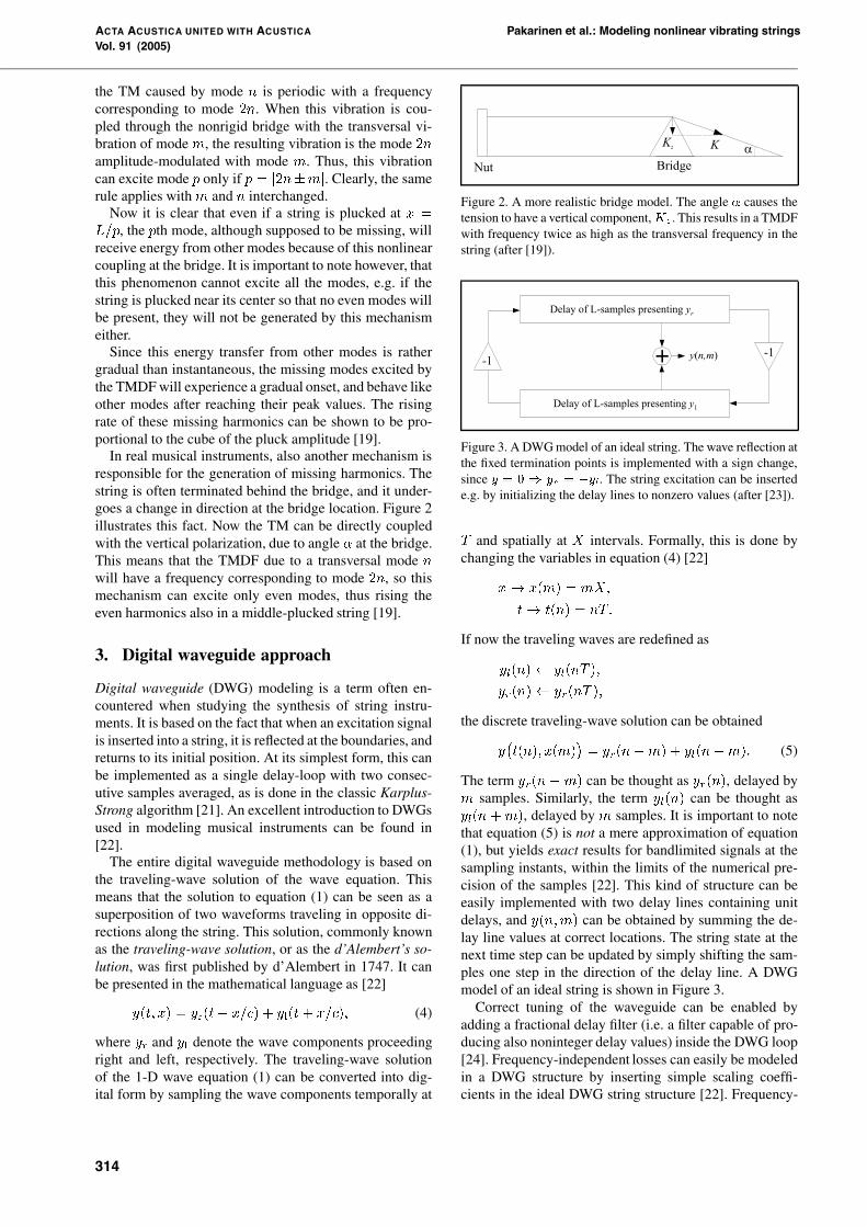
In real musical instruments, also another mechanism isresponsible for the generation of missing harmonics. Thestring is often terminated behind the bridge, and it under-goes a change in direction at the bridge location. Figure 2illustrates this fact. Now the TM can be directly coupledwith the vertical polarization, due to angle � at the bridge.This means that the TMDF due to a transversal mode nwill have a frequency corresponding to mode �n, so thismechanism can excite only even modes, thus rising theeven harmonics also in a middle-plucked string [19].

3. Digital waveguide approach

Digital waveguide (DWG) modeling is a term often en-countered when studying the synthesis of string instru-ments. It is based on the fact that when an excitation signalis inserted into a string, it is reflected at the boundaries, andreturns to its initial position. At its simplest form, this canbe implemented as a single delay-loop with two consec-utive samples averaged, as is done in the classic Karplus-Strong algorithm [21]. An excellent introduction to DWGsused in modeling musical instruments can be found in[22].

The entire digital waveguide methodology is based onthe traveling-wave solution of the wave equation. Thismeans that the solution to equation (1) can be seen as asuperposition of two waveforms traveling in opposite di-rections along the string. This solution, commonly knownas the traveling-wave solution, or as the d’Alembert’s so-lution, was first published by d’Alembert in 1747. It canbe presented in the mathematical language as [22]

y�t� x� � yr�t� x�c� � yl�t� x�c�� (4)

where yr and yl denote the wave components proceedingright and left, respectively. The traveling-wave solutionof the 1-D wave equation (1) can be converted into dig-ital form by sampling the wave components temporally at

BridgeNut

K�

Kz

Figure 2. A more realistic bridge model. The angle � causes thetension to have a vertical component, Kz . This results in a TMDFwith frequency twice as high as the transversal frequency in thestring (after [19]).

Delay of L-samples presenting y1

Delay of L-samples presenting yr

y n,m( )-1

-1

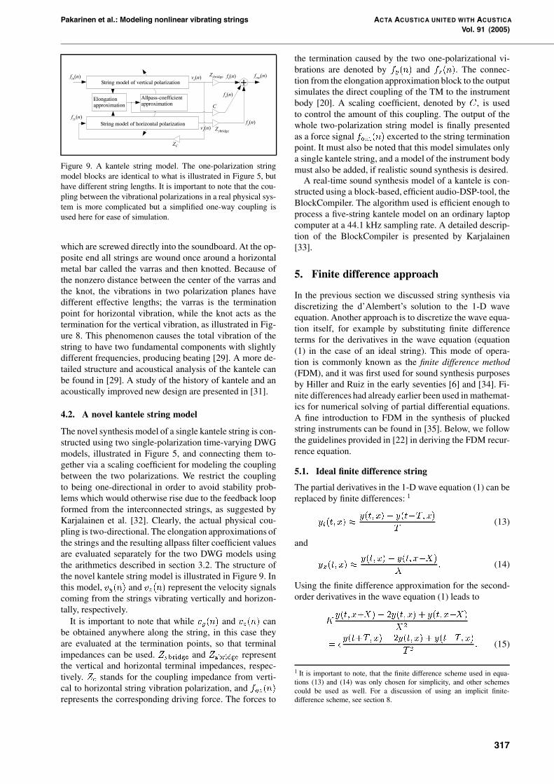
Figure 3. A DWG model of an ideal string. The wave reflection atthe fixed termination points is implemented with a sign change,since y � � � yr � �yl. The string excitation can be insertede.g. by initializing the delay lines to nonzero values (after [23]).

T and spatially at X intervals. Formally, this is done bychanging the variables in equation (4) [22]

x� x�m� � mX�

t� t�n� � nT�

If now the traveling waves are redefined as

yl�n�� yl�nT ��

yr�n�� yr�nT ��

the discrete traveling-wave solution can be obtained

y�t�n�� x�m�

�� yr�n�m� � yl�n�m�� (5)

The term yr�n �m� can be thought as yr�n�, delayed bym samples. Similarly, the term yl�n� can be thought asyl�n �m�, delayed by m samples. It is important to notethat equation (5) is not a mere approximation of equation(1), but yields exact results for bandlimited signals at thesampling instants, within the limits of the numerical pre-cision of the samples [22]. This kind of structure can beeasily implemented with two delay lines containing unitdelays, and y�n�m� can be obtained by summing the de-lay line values at correct locations. The string state at thenext time step can be updated by simply shifting the sam-ples one step in the direction of the delay line. A DWGmodel of an ideal string is shown in Figure 3.

Correct tuning of the waveguide can be enabled byadding a fractional delay filter (i.e. a filter capable of pro-ducing also noninteger delay values) inside the DWG loop[24]. Frequency-independent losses can easily be modeledin a DWG structure by inserting simple scaling coeffi-cients in the ideal DWG string structure [22]. Frequency-

314


dependent losses can in turn be simulated using lowpassfilters (a.k.a. loop filters) inside the DWG loop.

3.1. Time-varying digital waveguide string

When tension modulation is to be implemented in a stringmodel, it clearly means that the fundamental frequency ofthe string must be modulated also (see equation 2). In aDWG string this corresponds to varying either the lengthof the delay lines or the temporal sampling instant. Thissection discusses implementing the TM by varying thelength of the delay lines, and is presented earlier in a re-cent publication by the authors [3]. Since the delay linescan generally have integer-valued delays only, directly al-tering them would lead to having the tension change in astepwise manner. Obviously, this behavior is not desiredand therefore fractional delay (FD) elements are used. Foran in-depth study of FD elements, see [24].

A first-order allpass filter was chosen for the FD ele-ment of our string model.

A�z� ��a� z��

�� az�� (6)

where a is the filter coefficient which defines the length ofthe delay. Notice that when a � �, the allpass filter acts asa unit delay.

The decision for using a first-order allpass filter withinthe string model was done partly because it is the simplestway to design an allpass filter approximating a given frac-tional delay [24], and partly because the first-order allpassfilter is the best choice for the fractional delay elementwhen delay values around unity are to be obtained [25].The phase response error caused by the allpass filter is notconsidered to pose a problem since its effect is negligiblein the audio frequency range, assuming the sampling fre-quency to be reasonably high [26].

3.2. Distributed nonlinear DWG string

Previous works [27], [28], [29] use a single fractional de-lay element in a single-polarization string model, or aDWG string terminated with a nonlinear double-spring[30] to simulate the nonlinear string. This is done in or-der to reduce the computational complexity of the model,but it has also some shortcomings. Since the system is non-linear, the FD elements cannot be lumped into one singleelement without giving up the idea of viewing the systemas a distributed model.

In other words, the whole string becomes a lumpedmodel, and the termination point “behind” the FD elementbecomes the only location for gathering meaningful outputfrom the string. Physically this would correspond to a sin-gle elastic element at the termination point of an otherwiserigid string. A more realistic solution can be obtained if theelongation process is distributed along the delay line, in asimilar way as in a real physical string, where the elasticityis distributed along the string, rather than lumped.

The distributed nonlinearity can be implemented by ex-changing the delay lines of the DWG model of Figure 3

gz

-1

A z( )

v n( )/s( )n

+/-g

(a) (b)

Figure 4. Illustration of (a) a basic element, and (b) how to getoutput data from a string consisting of these elements. The di-rections of the wave components in (a) are opposite for adjacentelements, so that in effect the unit delays and allpass filters areinterleaved for each delay line. In (b), either the velocity or theslope of the string segment can be obtained, if velocity is used asthe wave variable.

F n( )

y n( )

HL

HR

Figure 5. One-polarizational DWG string with time-varyinglength. The string consists of the basic elements illustrated inFigure 4(a). HL and HR denote the loop filters simulating thefrequency-dependent losses. The excitation to the string can beinserted as a force signal using an interaction element, denotedby I . The construction of the interaction element is illustrated inFigure 6.

F n( )

F n( )

y n( )v n( )

2Z12Z2

Z2Z1

y n( )

Figure 6. The interaction element allows excitation signals to beinserted to the string during run-time. The input signal F �n� canbe seen as a force signal, and the output signal y�n� as a dis-placement signal. The coefficients Z� and Z� represent the me-chanical impedances of the two string branches. Implementationof the integrator block is depicted in Figure 7.

with a structure consisting of allpass filters. Then the ef-fective length of the delay lines can be changed by vary-ing the filter coefficients. We will now introduce a de-lay block which contains a unit delay, a first-order all-pass filter, and two scaling coefficients for modeling thefrequency-independent losses. This block is called a basicelement, and it is illustrated in Figure 4(a). The unit delayin each basic element ensures that no delay-free loops are

315


formed when constructing models using these elements.Figure 4(b) shows how to obtain output data from a junc-tion between two basic elements. A time-varying DWGstructure consisting of these elements is illustrated in Fig-ure 5.

From the discussion in section 1, we can conclude that asuitable control signal for the FD elements can be derivedfrom the instantaneous elongation of the string. In the fol-lowing, since the longitudinal wave propagation velocityis considerably higher than the transversal wave velocity,we will assume that the longitudinal waves will propa-gate instantaneously through the string, and the elongationcalculation and the FD parameter tuning can be done forthe whole string in one piece. In practice, the longitudinalwave velocity is typically only 5-20 times higher than thetransversal one, but carrying out the FD parameter evalua-tions for multiple string segments would add a significantcomputational load, likely without any audible advances.The elongation of the string can be expressed as [19]

ldev�t� �

Z lnom

�

q� �

�yx�t� x�

��dx � lnom� (7)

where lnom is the nominal string length, x is the spatial co-ordinate along the string, and y is the displacement of thestring. The first spatial derivative, yx, suggests the use ofslope waves in the elongation calculation, and thus equa-tion (7) can be approximated for the digital waveguide as[28]

Ldev�n� �

�LnomXm��

p� � �sr�n�m� � sl�n�m�� Lnom� (8)

where sr�n�m� and sl�n�m� are the slope waves at timeinstant n and position m, propagating to the right and tothe left, respectively. Lnom is the rounded nominal stringlength. To reduce the computational complexity, equation(8) can be further simplified using a truncated Taylor seriesexpansion to [28]

Ldev�n� ��

�

�LnomXm��

�sr�n�m� � sl�n�m�

�� (9)

while still maintaining a sufficient accuracy. The approx-imated delay variation of the total DWG can be obtainedfrom equation (9) as [28]

Ddev�n� � ��

�

n��Xl�n��Lnom

��

EA

K�

�Ldev�l�

Lnom� (10)

where E is Young’s modulus, A is the cross-sectional areaof the string, and K� is the nominal tension correspond-ing to the string at rest. The length of the string in samplesis denoted as Lnom � lnomfs�cnom, where fs is the tem-poral sampling frequency and cnom is the nominal wavepropagation speed.

T

z-1

Figure 7. The integrator block is implemented by summing upconsecutive samples.

Figure 8. Illustration of the kantele. The string termination at var-ras is magnified for clarity. A denotes the termination point forvertical vibration of the string, while B denotes the terminationpoint for horizontal vibration.�l stands for the distance betweenA and B.

Since the system under consideration uses a distributedset of delay elements, the desired delay for each basic ele-ment is

dpartial � � �Ddev

Lnom

� (11)

The coefficient a in equation (6) can now be expressed as[26, 24]

a �dpartial � �

dpartial � �� (12)

where dpartial is the delay intended for a single allpass fil-ter. Note that previous studies have used a different signfor a in equations (6) and (12), although the operation ofthe allpass filter remains the same.

4. Synthesis model of the kantele usingnonlinear digital waveguides

In this section, we demonstrate the nonlinear DWG for-mulation by constructing a two-polarizational synthesismodel of the kantele, a Finnish folk music instrument.

4.1. Acoustical analysis of the kantele

The kantele is a bridgeless plucked string instrument withusually five metal strings in its basic form (see Figure 8).The strings are terminated at one end by metal tuning pins,

316


f nin

( ) f nout

( )

f ny( )

f nx( )

f nzy

( )

f nz( )v n

z( )

v ny( )

ZC

Zybridge

Zzbridge

C

Figure 9. A kantele string model. The one-polarization stringmodel blocks are identical to what is illustrated in Figure 5, buthave different string lengths. It is important to note that the cou-pling between the vibrational polarizations in a real physical sys-tem is more complicated but a simplified one-way coupling isused here for ease of simulation.

which are screwed directly into the soundboard. At the op-posite end all strings are wound once around a horizontalmetal bar called the varras and then knotted. Because ofthe nonzero distance between the center of the varras andthe knot, the vibrations in two polarization planes havedifferent effective lengths; the varras is the terminationpoint for horizontal vibration, while the knot acts as thetermination for the vertical vibration, as illustrated in Fig-ure 8. This phenomenon causes the total vibration of thestring to have two fundamental components with slightlydifferent frequencies, producing beating [29]. A more de-tailed structure and acoustical analysis of the kantele canbe found in [29]. A study of the history of kantele and anacoustically improved new design are presented in [31].

4.2. A novel kantele string model

The novel synthesis model of a single kantele string is con-structed using two single-polarization time-varying DWGmodels, illustrated in Figure 5, and connecting them to-gether via a scaling coefficient for modeling the couplingbetween the two polarizations. We restrict the couplingto being one-directional in order to avoid stability prob-lems which would otherwise rise due to the feedback loopformed from the interconnected strings, as suggested byKarjalainen et al. [32]. Clearly, the actual physical cou-pling is two-directional. The elongation approximations ofthe strings and the resulting allpass filter coefficient valuesare evaluated separately for the two DWG models usingthe arithmetics described in section 3.2. The structure ofthe novel kantele string model is illustrated in Figure 9. Inthis model, vy�n� and vz�n� represent the velocity signalscoming from the strings vibrating vertically and horizon-tally, respectively.

It is important to note that while vy�n� and vz�n� canbe obtained anywhere along the string, in this case theyare evaluated at the termination points, so that terminalimpedances can be used. Zybridge and Zzbridge representthe vertical and horizontal terminal impedances, respec-tively. Zc stands for the coupling impedance from verti-cal to horizontal string vibration polarization, and fyz�n�represents the corresponding driving force. The forces to

the termination caused by the two one-polarizational vi-brations are denoted by fy�n� and fz�n�. The connec-tion from the elongation approximation block to the outputsimulates the direct coupling of the TM to the instrumentbody [20]. A scaling coefficient, denoted by C, is usedto control the amount of this coupling. The output of thewhole two-polarization string model is finally presentedas a force signal fout�n� excerted to the string terminationpoint. It must also be noted that this model simulates onlya single kantele string, and a model of the instrument bodymust also be added, if realistic sound synthesis is desired.

A real-time sound synthesis model of a kantele is con-structed using a block-based, efficient audio-DSP-tool, theBlockCompiler. The algorithm used is efficient enough toprocess a five-string kantele model on an ordinary laptopcomputer at a 44.1 kHz sampling rate. A detailed descrip-tion of the BlockCompiler is presented by Karjalainen[33].

5. Finite difference approach

In the previous section we discussed string synthesis viadiscretizing the d’Alembert’s solution to the 1-D waveequation. Another approach is to discretize the wave equa-tion itself, for example by substituting finite differenceterms for the derivatives in the wave equation (equation(1) in the case of an ideal string). This mode of opera-tion is commonly known as the finite difference method(FDM), and it was first used for sound synthesis purposesby Hiller and Ruiz in the early seventies [6] and [34]. Fi-nite differences had already earlier been used in mathemat-ics for numerical solving of partial differential equations.A fine introduction to FDM in the synthesis of pluckedstring instruments can be found in [35]. Below, we followthe guidelines provided in [22] in deriving the FDM recur-rence equation.

5.1. Ideal finite difference string

The partial derivatives in the 1-D wave equation (1) can bereplaced by finite differences: 1

yt�t� x� �y�t� x�� y�t�T� x�

T(13)

and

yx�t� x� �y�t� x�� y�t� x�X�

X� (14)

Using the finite difference approximation for the second-order derivatives in the wave equation (1) leads to

Ky�t� x�X�� y�t� x� � y�t� x�X�

X�

� �y�t�T� x�� y�t� x� � y�t�T� x�

T �� (15)

1 It is important to note, that the finite difference scheme used in equa-tions (13) and (14) was only chosen for simplicity, and other schemescould be used as well. For a discussion of using an implicit finite-difference scheme, see section 8.

317


Solving (15), we get

y�t�T� x� �KT �

�X�

�y�t� x�X�� y�t� x� � y�t� x�X�

�� y�t� x�� y�t�T� x�� (16)

Next, we define the relationship between the spatial andtemporal sampling steps with [35]

r � cT

X� �� (17)

where the “less than unity”-restriction is called the VonNeumann stability condition. Using this together with thedefinition of transversal wave velocity (equation 2), equa-tion (16) can be written as

y�t�T� x� � r��y�t� x�X� � y�t� x�X�

�(18)

� �� r��y�t� x�� y�t�T� x��

If we now do the discretization by denoting t � t�n� �nT and x� x�m� � mX , as we did in section 3, we endup with the finite difference approximation [35]

y�n��m� � r��y�n�m�� y�n�m��

�(19)

� �� r��y�n�m�� y�n��m��

If we set r � �, (19) becomes

y�n��m� � y�n�m�� y�n�m��

� y�n��m�� (20)

which is the finite difference equation of an ideal string.The equality of equation (20) can be checked by substitut-ing the waveguide decomposition (equation 5) in the right-hand side of equation (20) [22].

Since the length of the string must again have integervalues, correct tuning of the string becomes difficult. It hasbeen shown [35] that choosing r � � in equation (17) re-sults in lowering the fundamental frequency of the string.Therefore, the finite difference string can be tuned via theparameter r.

Choosing r � � also gives raise to an unwanted nu-merical dispersion phenomenon called grid dispersion [7],where the wave velocity in the numerical implementationwill be less than the ideal physical wave velocity. This ar-tificial dispersion affects primarily the upper harmonics,where the frequencies will be underestimated. If a typi-cal error of �� in the generated frequencies is allowed,the difference between the tuning coefficient r and unityshould not be greater than �� [35]. If the constraints be-tween the correct tuning and grid dispersion do not yieldsatisfactory results, the spatial density of the grid shouldbe increased. This is known as spatial oversampling.

5.2. Boundary conditions and string excitation

Since the spatial coordinate m of the string must liebetween � and Lnom, problems arise near the ends ofthe string when evaluating equation (20) because spatialpoints outside the string are needed. The problem can

be solved by introducing boundary conditions that definehow to evaluate the string movement when m � � orm � Lnom. The simplest approach, introduced alreadyin [6], would be to assume that the string terminations berigid, so that y�n� �� y�n� Lnom� � �. This results in aphase-inverting termination, which suits perfectly the caseof an ideal string. For other types of string termination,several models have been introduced (see e.g. [6], [35],and [36]). Generally, the nonrigid string terminations leadto frequency-dependent losses in the string model.

For the FDM string excitation, a useful method has beenproposed in [36]. It is conceptually simple and allows forinteraction with the string during run-time. There,

y�n�m�� y�n�m� ��

�u�n� (21)

and

y�n�m�� y�n�m��

�u�n� (22)

are inserted into the string, which causes a “boxcar” blockfunction to spread in both directions from the excitationpoint pair. The wave component u�n� is now used as theexcitation signal in a similar way as the exciting force sig-nal F �n� in section 3.2.

5.3. Finite difference approximation of a lossy string

Frequency-independent losses can be modeled in an FDMstring by discretizing the velocity-dependent dampingterm in the lossy 1D wave equation (3). This results in twoadditional scaling coefficients in the recurrence equation[35]

y�n��m� � p�y�n�m�� y�n�m��

�� qy�n��m�� (23)

where the values of p and q determine the amount oflosses. Generally, p and q may depend on the spatial indexm, but since homogeneous strings are considered here, thisdependency is omitted. Values

q � p� � jpj � � (24)

ensure the stability of a linear finite difference string withfrequency-independent losses [37]. Note that the sign dif-ference of p and q in [37] has already been taken care ofin equation (23). Modeling of frequency-dependent lossesby discretizing the lossy wave equation leads to an implicitrecurrence equation, which can be evaluated, if suitableapproximations are made [35].

6. Nonlinear finite difference string

Implementing tension modulation in a digital waveguidestring in section 3 was not an overly difficult task. This wasdue to the fact that the implementation of a DWG string isessentially a feedback loop with delay, and therefore mod-ulating the delay time of this loop corresponded to modu-lating the wave velocities. In FDM strings, however, such

318


Figure 10. Illustration of the nonlinear FD algorithm on a spatio-temporal grid. The vertical axis denotes the time, while the hor-izontal axis denotes the spatial location on the string. The illus-tration is shown only for a string segment of length N � �, forclarity. In each step of the algorithm, most recently evaluated val-ues are presented as black dots, while earlier values are presentedas white dots.

an approach would not lead to satisfactory results, sincethe physical quantities (e.g. displacement) themselves arepresent in the string model, and not their wave decompo-sitions2.

Instead, we concluded that in order to correctly modelthe TM in a FDM string, we first have to evaluate the recur-rence equation and use these three snapshots of the string(at time instants n��, n, and n��) in interpolating two newstring states at time instants n�� and n�� , where� � � � �. Using these two string states we then eval-uate the recurrence equation, in order to obtain the stringstate at time n�� . It is important to note that the in-terpolation here is in effect stretching the time axis so thatthe wave propagation velocities are altered, whereas in theDWG model the allpass filters perform the interpolation inthe spatial domain.

This algorithm can also be seen as using two FDM sys-tems in implementing the nonlinear string. The elongationof the string would be evaluated from one system, and theresult, the stretched string state, would be updated to theother system. Figure 10 illustrates this procedure on thespatio-temporal grid.

In step 1, the two initial states have been assigned forthe string, and the state at the next instant (in the linearcase) is obtained by the standard recurrence equation (20).The grid values which represent the state of the string atthe corresponding time instant are circled in step 1. In step2, sample values corresponding to the TM have been inter-polated from the string states in step 1. In step 3, equation(20) has been applied on the values evaluated in step 2, in

2 Such a system which deals with the physical quantities themselves iscalled a Kirchhoff model, as opposed to a wave model, which deals withthe wave components of the physical quantities.

(c)

(b)

(a)

t

t

t t

t

t

n

n

n n

n

n

n+1

n+1

n+1 n+1

n+1

n+1y n+ m( 1, )

y n+ m( 1, )

y n m( , )

y n m( , )

y n+ m( 1, )

y n- m( 1, )

m

m

m m

m

m

d

d

d

a

a

a

-a

-a

-a

z-1

z-1

z-1

n-1

n-1

n-1 n-1

n-1

n-1

Figure 11. Illustration of the interpolation process due to thechange in the string’s length. The spatio-temporal grids on theleft and right represent the linear and interpolated string states,respectively. The fractional delay value caused by the interpola-tion is denoted by d. The interpolation process in (a) is simplifiedin (b), and further in (c).

order to obtain the string state corresponding to the changein tension. The two most recently obtained states are nowtaken as the “initial states” in step 4, and we can return tostep 1.

As seen in Figure 10, the tension modulation corre-sponds here to interpolating the string state in the tempo-ral domain. The elongation of the FDM string was evalu-ated similarly to what was done in equation (9), except thathere the slope of the string was obtained by taking the dif-ference of the displacements between two adjacent stringsegments, rather than summing up the slope wave compo-nents. In the following, we will have a closer look at theinterpolation process.

6.1. String state interpolation

We chose again to use first-order allpass filters in inter-polating the string state from the linear model (step 2 inFigure 10). Figure 11(a) illustrates how the interpolatedvalue of y�n�m� is obtained from the linear values. Thespatio-temporal grid on the left represents the string statein the linear case, while the spatio-temporal grid on theright represents the string state after spatial interpolation.The structure between the two grids is the block diagramof a first-order allpass filter (equation 6). The coefficient afor the allpass filter was evaluated as presented earlier byequations (9)–(12).

319


In this figure, we notice that the allpass filter uses thevalue of y�n��m� delayed by one sample, thus corre-sponding to y�n�m�. Clearly, this can be obtained directlyfrom the grid on the left, and the branch on the left contain-ing the unit delay can be reformed. The result is shown inFigure 11(b). Here we also note that the interpolation sys-tem uses its own output at the previous time instant. This isactually the same as using the value of y�n��m�, becauseit is the same as the output of the interpolation process onetime step ago (this might be best understood by noting thatthe bottom row of step 4 in Figure 10 is the same as thebottom row of step 1 at the next time instant). Thus, Fig-ure 11(b) can be further simplified to Figure 11(c).

Having this said, the recurrence equation for the time-varying finite difference string with frequency-indepen-dent damping can be written as

y��n��m� � p�y��n�m�� y��n�m��

�� qy��n��m�� (25)

where

y��n�m�� ay��n��m�� y��n�m��

� ay��n��m��

y��n�m�� ay��n��m�� y��n�m��

� ay��n��m��

y��n��m� � �ay��n�m� � y��n��m�

� ay��n� ��m��

Here the coefficients p and q incorporate the frequency-independent losses and y� and y� refer to the linear and in-terpolated strings, respectively. Simplifying and rearrang-ing we end up with an equation containing only terms ofy�, and the subscript may therefore be omitted

y�n��m� � �pay�n��m�� pay�n��m��

� py�n�m�� qay�n�m� � py�n�m��

� pay�n��m�� qy�n��m�

� pay�n��m�� qay�n� ��m�� (26)

This equation is illustrated with a block diagram in Fig-ure 12 along with its abstraction. A nonlinear FDM stringcan be constructed by connecting several of these blockstogether and using the string elongation in controlling theamount of interpolation. We will refer to such a block asa time-varying finite difference time-domain (FDTD) ele-ment. Illustration of the lossless time-varying FDTD ele-ment can be found in Figure 13, where p and q equal unityand have therefore been left out.

6.2. String excitation and termination

For the interaction with the time-varying FDTD stringmodel, we chose to use the “boxcar” excitation model dis-cussed in section 5.2, so that the excitation signal couldagain be interpreted as a force signal. Figure 14 presentsan interaction block to be used with a time-varying FDTDstring. We will call such a block the FDTD interaction el-

FDTD

-pa

z-1

z-1

z-1

y n+1,m( )

y n,m( )

y n-2,m( )

y n-1,m( )

-pa

pa

qa

-q

-qa

pa

p p

Figure 12. Illustration of the time-varying FDTD element to-gether with its abstraction. A lossless time-varying FDTD ele-ment can be found in Figure 13.

-a

z-1

z-1

z-1

y n-1,m( )

y n-2,m( )

y n,m( )

y n+1,m( )

-a

-a

a

a

a

Figure 13. Illustration of the lossless time-varying FDTD ele-ment.

ement. Using these DSP blocks, we can construct a one-polarization nonlinear FDTD (NFDTD) string, as illus-trated in Figure 15.

We chose to use rigid terminations for our nonlin-ear finite difference string model, since the modeling offrequency-dependent losses is not a key aspect of thisstudy. Fixed terminations do not ruin the generation ofmissing harmonics in our model either, since the TMDFcoupling is implemented in a different manner, as ex-plained below.

6.3. NFDTD string with generation of missing har-monics

In order to model the generation of missing harmonics ina NFDTD string, we constructed a model, where an addi-tional interaction element is placed between the last FDTDelement and the termination for feeding the TMDF to thestring. Since the spatial distance between the last FDTD

320


y n-1,m+1( )

y n-1,m( )

F n( )

F n( )

y n,m+1( )

y n,m( )

y n+1,m+1( )

y n+1,m( )

Figure 14. Illustration of the FDTD interaction element togetherwith its abstraction. The excitation algorithm is defined by equa-tions (21) and (22).

F n( )

FDTD FDTD FDTD FDTD FDTD

Allpass-coefficientapproximation

Elongationapproximation

Figure 15. One-polarizational NFDTD string. The string consistsof the time-varying FDTD elements illustrated in Figure 12. Thezero-blocks at the terminations give zero as an output regardlessof the input values, thus implying a rigid termination. The excita-tion to the string can be inserted as a force signal using a FDTDinteraction element, illustrated in Figure 14.

F n( )

FDTD FDTD FDTD

TMDF

FDTD

Allpass-coefficientapproximation

Elongationapproximation

y n L( , -1)nom

�

Figure 16. Illustration of the NFDTD string with a generationmechanism for missing harmonics. A second interaction elementis added in order to feed the TMDF into the string. The scal-ing coefficient �TMDF controls the amplitude of the missing har-monics. The string elongation is approximated from the displace-ments of each FDTD element.

element and the rigid termination is one sample, the ver-tical component of the TMDF can be seen to be equal tothe product of the displacement of the last FDTD elementand the tension. Here, we can replace the tension signalby the elongation signal, and introduce a scaling coeffi-cient �TMDF to control the amount of TMDF to be in-serted to the interaction element at the termination. Thisis illustrated in Figure 16. The generation of missing har-

monics in a NFDTD model will be further discussed in thefollowing section.

7. Simulation results

In this section we present the results obtained from the twononlinear string algorithms, discussed in sections 3 and 5.The synthesis results are compared by simulating the samephenomena, namely the initial pitch glide and the genera-tion of missing harmonics, using the two models. Stabilityissues and computational cost of the synthesis models arealso discussed.

7.1. Synthesis results

The synthesis results reveal that both the nonlinear DWGand NFDTD models are able to realistically model the ini-tial pitch glide phenomenon. Figure 17 illustrates the fun-damental frequency behavior of a recorded kantele toneand the two synthesized tones. Here, the horizontal dottedline approximates the mean value of perceptual detectionthreshold of an initial pitch glide. The psychoacoustic de-tection threshold in the frequency region of these tones isabout 5.4 Hz [38]. This shows that the fundamental fre-quency glide is an audible phenomenon in plucked stringinstruments such as the kantele even at modest pluckingamplitudes, and thus it must be included in a synthesismodel if realistic tones are desired.

The nonlinear DWG model used in this figure has a totaldelay line length of 55.125 samples and the allpass coef-ficient a is scaled using a constant value of 0.9 in orderto correctly simulate the behavior of the recorded sample.The NFDTD string consists of 56 FDTD elements, andthe fine-tuning parameter (a.k.a. Courant number, equa-tion 17) has a value of r � �� . The allpass coefficienta is scaled using a coefficient �� in the NFDTD case.

The modeling of the generation of missing harmonicscan be implemented similarly in the distributed nonlinearDWG model as was suggested in [28]. If the boxcar inte-gration of equation (10) is replaced with a leaky integratorhaving the transfer function

I�z� � gp� � ap

� � apz�� (27)

the generation of the missing harmonics can be controlledvia the integration parameter ap. The variable gp definesthe gain of the integration.

Figure 18 shows the amplitude envelopes of the firstthree harmonics of a synthesized tone with two differ-ent ap parameter values. The string was plucked close to��rd of its length, and as can be seen in the figure, themissing harmonic in (a) has a gradual increase after thebeginning transient, after which it experiences an expo-nential decay like all other modes.

It is worthwhile to note that the generation of missingharmonics in the nonlinear DWG model results from theproperties of the integration of the elongation approxima-tion, and is therefore not a physically justified process. Ba-sically, here the integration error in the leaky integrator is

321


Time [s]

fnom

Fre

quen

cy[H

z]

Figure 17. Fundamental frequencies as a function of time fora moderately-plucked recorded kantele tone (solid line), a syn-thesized nonlinear DWG tone (dashed line), and a synthesizedNFDTD tone (dash-dotted line). The fnom stands for the nomi-nal fundamental frequency of the string, and the horizontal dottedline denotes the approximated detection threshold of a pitch drift(fnom��Hz), which suggests that the fundamental frequencydrifts in all cases are audible.

responsible for feeding energy to the missing harmonics.Also, unlike the real physical phenomenon, the generationof missing harmonics in the nonlinear DWG case does notdepend on the rigidity of the terminations. Nevertheless,this feature can be exploited in emulating the real stringbehavior, when the integration parameters are properly ad-justed. Details on tuning the leaky integrator parameterscan be found in [28].

Modeling the generation of missing harmonics in aNFDTD string is however not so simple. Even if a leakyintegrator is used in the elongation calculation, its param-eters do not have a desirable effect on the missing har-monics. This does not seem too surprising when consider-ing the major differences of these two algorithms and it isthe reason that forced us to use an alternative mechanismfor creating the missing harmonics in the previous section(Figure 16).

Figure 19 represents the behavior of the first three har-monics of a tone synthesized by this model. It can be seenthat the missing harmonics can be “lifted” by choosing aproper value for �TMDF. The stability of the system how-ever poses an upper limit for the �TMDF coefficient, sincethe TMDF mechanism continuously feeds energy to thestring. According to our experience, generating missingharmonics with amplitudes greater than what is shown inFigure 19 is difficult.

7.2. Stability issues and computational comparison

We found the nonlinear DWG algorithm to remain sta-ble for nearly all parameter and excitation values. Onlyhighly exaggerated nonlinearity scaling values togetherwith high excitation impulses resulted in stability prob-lems. We thus conclude that the nonlinear DWG waveg-uide has no real stability problems when synthesis of nat-ural plucked-instrument sounds are desired.

We studied the stability of the NFDTD algorithm us-ing the Von Neumann analysis [39] in the time-invariantcase, i.e. parameter a of equation (26) was kept constant.The basic idea of this method is to calculate the spatialFourier spectrum of the system under discussion at twoconsecutive time steps. An amplification function�, which

(a)

(b)

Figure 18. Generation of the missing harmonics in the nonlinearDWG model can be controlled via the leaky integrator parame-ters. Here, the string was plucked approximately at ��rd of itslength, so every 3rd harmonic should be missing from the re-sulting spectrum. In a), ap � �� and the third harmonicclearly rises after the initial transient. In b), ap � �� andthe third harmonic is more attenuated.

(a)

(b)

Figure 19. Generation of missing harmonics in a NFDTD string.The string was plucked again approximately at ��rd of itslength, and the coupling of the TMDF to the transversal vibra-tion was controlled using a scaling coefficient �TMDF. In a), thescaling coefficient has a value of �TMDF � �, and the missingthird harmonic can be seen rising after the initial transient. In b),�TMDF � �, and generation of missing harmonics does not takeplace.

shows how the spatial spectrum evolves with time, canthen be derived from the two spectra. If the absolute valueof this amplification function remains below unity, stabil-ity is guaranteed. Formally, the Von Neumann analysis forthe NFDTD algorithm goes as follows [4]:

If the spatial inverse Fourier transform is defined as

y�n�m� � FfY �n� ��g�� neim�� (28)

322


where is the spatial frequency and i is the imaginaryunit, the nonlinear finite-difference recurrence equation(26) can be written as

�n��eim� � �pa�n��ei�m�� pa�n��ei�m��

� p�nei�m�� qa�neim� � p�nei�m��

� pa�n��ei�m�� q�n��eim�

� pa�n��ei�m�� qa�n��eim�� (29)

Dividing with �n��eim� and rearranging, we have

�� paei� � pae�i��

� ��pei� � qa� pe�i��

� ��paei� � q � pae�i�� qa � �� (30)

Using the Euler’s equation leads to a simpler form

A� �B�� C��D � �� (31)

where

A � � � �pa cos��

B � �qa� �p cos��

C � q � �pa cos��

D � �qa� (32)

In order to get the amplification function �, we would nowhave to solve the third-order equation (31). Unfortunately,the solution of this equation is complicated and involvesdozens of terms. If we want to consider the stability of thelossless NFDTD string, we can substitute p � q � �. Thissimplifies the solution of equation (31) enough to enablenumerical stability analysis for the amplification function.The absolute value of the amplification function � is il-lustrated in Figure 20 as a function of the interpolationcoefficient a, and the spatial frequency .

It is important to note that this stability analysis is con-ducted on a lossless NFDTD string with constant inter-polation coefficient. We can thus call this system time-invariant (normally the interpolation coefficient dependson the string elongation).

Figure 20 reveals that in the lossless case, the time-invariant version of the NFDTD algorithm is unstable forall but very small a parameter values. Making the algo-rithm time-variant results in an even more unstable system.In a practical lossy string implementation, however, theNFDTD string remained stable for normal excitation am-plitudes (i.e. excitation amplitudes commonly used whenplaying real string instruments).

The computational complexities of the two algorithmsare different. Since the models consist mainly of the basicstring blocks (basic elements in the DWG case and FDTDelements in the finite difference case), the differences inthe computation of the basic string blocks dominate thecomputational needs of the algorithms.

The basic element (Figure 4) consists of four multipli-cations and two summations per time sample, whereas theFDTD element (Figure 12) requires a total of nine multi-plications and eight summations for computing one time

a

Figure 20. Absolute value of amplification function of a NFDTDalgorithm. The white color denotes areas where the amplificationfunction exceeds unity, i.e. when the model becomes unstable.

sample. Although the interaction and termination blocksare much simpler in the finite difference case, the typi-cally large number of the string elements turns the favorto the nonlinear DWG model. If the computational cost ofthe string elongation approximation is taken into account,the NFDTD algorithm can be seen to have twice the com-putational complexity of its digital waveguide counterpart.For a more thorough comparison of the two presented al-gorithms, see [4].

8. Conclusions and future work

Two algorithms for modeling spatially distributed non-linear strings in a physically meaningful way were pre-sented: a nonlinear digital waveguide algorithm and a non-linear finite difference algorithm. The former uses first-order allpass filters distributed along a delay line for mod-ulating the total delay of the string loop, while the latterone uses first-order allpass filters for interpolating betweentime samples in the linear recurrence equation. Both tech-niques evaluate the control signals for the allpass filtersfrom the elongation of the string. The amount of nonlin-earity, among with other physical parameters, can be ad-justed in both string models. A physical model of a kantelestring was presented using the nonlinear digital waveguidestring algorithm.

Realistic simulation of the inital pitch glide phenome-non can be performed with both algorithms, but model-ing of the generation of missing harmonics can be realisti-cally obtained only using the nonlinear digital waveguidemodel, due to stability problems of the nonlinear finite dif-ference algorithm. Computational complexities of the twoalgorithms were also compared.

As stated in section 5.1, the explicit finite differencescheme was chosen for simplicity. Another option wouldbe to use an implicit scheme, such as a scheme [40],where the temporal and spatial derivatives of the waveequation (equation 1) are averaged in space and time, re-

323


spectively. Using such a scheme would lead to an uncon-ditionally stable finite difference algorithm and thus lib-erate us from the Von Neumann stability condition (equa-tion 17). The implicit form of this scheme would howevercall for a matrix formulation instead of a simple recurrenceequation, and probably increase the computational load ofthe algorithm. Construction of such an algorithm is left forfuture work.

AcknowledgementThanks to Dr. Cumhur Erkut and Dr. Lutz Trautmann forsuggestions and discussions. This work was supported bythe ALMA project (IST-2001-33059), the Academy ofFinland project SA 104934, and the Helsinki GraduateSchool of Electrical and Communications Engeneering.

References

[1] M. Karjalainen, C. Erkut: Digital waveguides vs. finitedifference schemes: Equivalence and mixed modeling.EURASIP Journal on Applied Signal Processing (June2004) 978–989. Special issue on Model-Based Sound Syn-thesis.

[2] C. Erkut, M. Karjalainen: Finite difference method vs. dig-ital waveguide method in string instrument modeling andsynthesis. Proceedings of the International Symposiumon Musical Acoustics (ISMA 2002), Mexico City, Mexico,December 9-13, 2002.

[3] J. Pakarinen, M. Karjalainen, V. Valimaki: Modeling andreal-time synthesis of the kantele using distributed tensionmodulation. Proc. Stockholm Music Acoustics Conference,Stockholm, Sweden, August 6-9, 2003, 409–412.

[4] J. Pakarinen: Spatially distributed computational modelingof a nonlinear vibrating string. Diploma Thesis. HelsinkiUniversity of Technology, June 14, 2004. Available on-lineat http://www.acoustics.hut.fi/publications/.

[5] N. H. Fletcher, T. D. Rossing: The physics of musical in-struments. Springer-Verlag, New York, USA, 1988.

[6] L. Hiller, P. Ruiz: Synthesizing musical sounds by solvingthe wave equation for vibrating objects: Part I. Journal ofthe Audio Engineering Society 19 (June 1971) 462–470.

[7] A. Chaigne, A. Askenfelt: Numerical simulations of pianostrings. I. A physical model for a struck string using finitedifference methods. Journal of the Acoustical Society ofAmerica 95 (February 1994) 1112–1118.

[8] M. Podlesak, A. Lee: Dispersion of waves in piano strings.Journal of the Acoustical Society of America 83 (1988)305–317.

[9] D. Hall: Piano string excitation in the case of small ham-mer mass. Journal of the Acoustical Society of America 79(1986) 141–147.

[10] D. Hall: Piano string excitation II: General solution for ahard narrow hammer. Journal of the Acoustical Society ofAmerica 81 (1987) 535–546.

[11] D. Hall: Piano string excitation III: General solution for asoft narrow hammer. Journal of the Acoustical Society ofAmerica 81 (1987) 547–555.

[12] H. Suzuki: Model analysis of a hammer-string interaction.Journal of the Acoustical Society of America 82 (1987)1145–1151.

[13] X. Boutillon: Model for piano hammers: Experimental de-termination and digital simulation. Journal of the Acousti-cal Society of America 83 (1988) 746–754.

[14] M. E. McIntyre, J. Woodhouse: On the fundamentals ofbowed string dynamics. Acustica 43 (1979) 93–108.

[15] J. Woodhouse: Idealised models of a bowed string. Acus-tica 79 (1993) 233–250.

[16] L. Cremer: The physics of the violin. MIT Press, Cam-bridge, MA, 1983.

[17] H. A. Conklin: Generation of partials due to nonlinear mix-ing in a stringed instrument. Journal of the Acoustical So-ciety of America 105 (January 1999) 536–545.

[18] B. Bank, L. Sujbert: Modeling the longitudinal vibration ofpiano strings. Proc. Stockholm Music Acoustics Confer-ence, Stockholm, Sweden, August 6-9, 2003, 143–146.

[19] K. A. Legge, N. H. Fletcher: Nonlinear generation of miss-ing modes on a vibrating string. Journal of the AcousticalSociety of America 76 (July 1984) 5–12.

[20] T. Tolonen, C. Erkut, V. Valimaki, M. Karjalainen: Simula-tion of plucked strings exhibiting tension modulation driv-ing force. Proceedings of the International Computer MusicConference, Beijing, China, October 22-28, 1999, 5–8.

[21] K. Karplus, A. Strong: Digital synthesis of plucked-stringand drum timbres. Computer Music Journal 7 (1983) 43–55.

[22] J. O. Smith: Principles of digital waveguide models of mu-sical instruments. Applications of Digital Signal Processingto Audio and Acoustics, (M. Kahrs and K. Brandenburg,eds.) (February 1998) 417–466.

[23] J. O. Smith: Physical modeling using digital waveguides.Computer Music Journal 16 (Winter 1992) 74–87.

[24] T. I. Laakso, V. Valimaki, M. Karjalainen, U. K. Laine:Splitting the unit delay - tools for fractional delay filter de-sign. IEEE Signal Processing Magazine 13 (1996) 30–60.

[25] V. Valimaki, T. I. Laakso: Principles of fractional delay fil-ters. Proceedings of the IEEE International Conference onAcoustics, Speech and Signal Processing, Istanbul, Turkey,5-9 June 2000, 3870–3873.

[26] V. Valimaki: Discrete-time modeling of acoustic tubes us-ing fractional delay filters. Doctoral dissertation, HelsinkiUniv. of Technol., Acoustics Lab Report Series, Reportno. 37, 1995. Available on-line at http://www.acous-tics.hut.fi/publications/.

[27] V. Valimaki, T. Tolonen, M. Karjalainen: Plucked-stringsynthesis algorithms with tension modulation nonlinear-ity. Proceedings of the IEEE International Conference onAcoustics, Speech and Signal Processing, Phoenix, Ari-zona, March 15-19, 1999, 977–980.

[28] T. Tolonen, V. Valimaki, M. Karjalainen: Modeling of ten-sion modulation nonlinearity in plucked strings. IEEETransactions on Speech and Audio Processing 8 (May2000) 300–310.

[29] C. Erkut, M. Karjalainen, P. Huang, V. Valimaki: Acous-tical analysis and model-based sound synthesis of the kan-tele. Journal of the Acoustical Society of America 112 (Oc-tober 2002) 1681–1691.

[30] J. R. Pierce, S. A. Van Duyne: A passive nonlinear digitalfilter design which facilitates physics-based sound synthe-sis of highly nonlinear musical instruments. Journal of theAcoustical Society of America 101 (February 1997) 1120–1126.

[31] J. Polkki, C. Erkut, H. Penttinen, M. Karjalainen,V. Valimaki: New designs for the kantele with improvedsound radiation. Proc. Stockholm Music Acoustics Confer-ence, Stockholm, Sweden, August 6-9, 2003, 133–136.

324


[32] M. Karjalainen, V. Valimaki, T. Tolonen: Plucked-stringmodels: From the Karplus-Strong algorithm to digitalwaveguides and beyond. Computer Music Journal 22(1998) 17–32.

[33] M. Karjalainen: BlockCompiler: Efficient simulation ofacoustic and audio systems. Proc. 114th AES Convention,Amsterdam, The Netherlands, 22-25 March 2003.

[34] L. Hiller, P. Ruiz: Synthesizing musical sounds by solvingthe wave equation for vibrating objects: Part II. Journal ofthe Audio Engineering Society 19 (June 1971) 542–551.

[35] A. Chaigne: On the use of finite differences for musi-cal synthesis. Application to plucked stringed instruments.Journal d’Acoustique 5 (1992) 181–211.

[36] M. Karjalainen: 1-D digital waveguide modeling for im-proved sound synthesis. Proceedings of the IEEE Inter-national Conference on Acoustics, Speech and Signal Pro-cessing, Orlando, Florida, USA, May 13-17, 2002, 1869–1872.

[37] C. Erkut, M. Karjalainen: Virtual strings based on a 1-D FDTD waveguide model: Stability, losses, and travel-ing waves. Proceedings of the Audio Engineering Society22nd International Conference, Espoo, Finland, June 15-17, 2002, 317–323.

[38] H. Jarvelainen, V. Valimaki: Audibility of initial pitchglides in string instrument sounds. Proceedings of the In-ternational Computer Music Conference, Havana, Cuba,17-23 September 2001, 282–285. Available on-line athttp://lib.hut.fi/Diss/2003/isbn9512263149/article3.pdf.

[39] J. C. Strikwerda: Finite difference schemes and partial dif-ferential equations. Wadsworth, Brooks & Cole, California,USA, 1989.

[40] A. Chaigne, V. Doutaut: Numerical simulations of xylo-phones. I. Time-domain modeling of the vibrating bars.Journal of the Acoustical Society of America 101 (January1997) 539–557.

325

jyri€pakarinen,€vesa€välimäki,€and€matti€karjalainen,€2005...

Documents