k e y c o n ce p t: b in ary l ogistic r egression w ith...

Stat 504, Lecture 13 1!

"

#

$

Key Concept:

• Binary Logistic Regression with continuous

predictor


"

#

$

Binary Logistic Regression

Objective: Estimate the probability that a

characteristic is present (e.g. estimate probability of

”success”) given the value of explanatory variable(s)

Variables:

• Let Yi be a binary response variable

Yi =

8<:

1 if the trait is present in observation i

0 if the trait is NOT present in observ. i

• Xi be an explanatory variable for observation i;

it can be discrete and/or continuous.

Assumptions:

• The data Y1, Y2, ..., Yn are independently

distributed

• Distribution of Yi is Bin(ni,πi)

• πi = Pr(Yi = 1|Xi) =probability that the

characteristic is present in observation i given the

value of the explanatory variable Xi.


"

#

$

Model:

πi = Pr(Yi = 1|Xi) =exp(β0 + β1Xi)

1 + exp(β0 + β1Xi)

or

logit(πi) = log“ πi

1 − πi

”= β0 + β1Xi


"

#

$

Parameter Estimation:

The maximum likelhood estimator (MLE) for (β0,β1)

is obtained by finding (β0, β1) that maximizes

L(β0,β1) =NY

i=1

πyi

i (1−πi)ni−yi =

NYi=1

exp{yi(β0 + β1Xi)}1 + exp(β0 + β1Xi)

In general, there are no closed-form solutions, so the

ML estimates are obtained by using iterative

algorithms such as Newton-Raphson (NR), Iteratively

reweighted least squares (IRWLS), etc.

If you are interested in computational aspects of these

algorithms and how to implement them, a good

starting reference is:

http://www.stat.cmu.edu/∼minka/papers/logreg/

In Agresti, see 4.6.1 and for logistic regression

5.5.4-5.5.5.


"

#

$

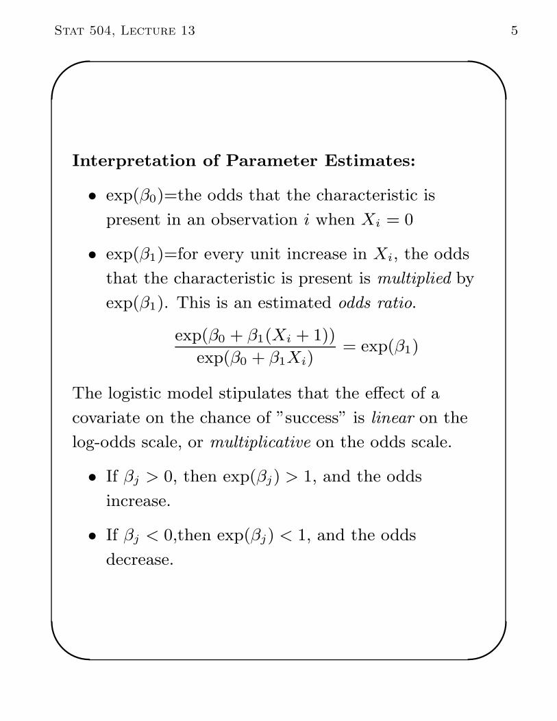
Interpretation of Parameter Estimates:

• exp(β0)=the odds that the characteristic is

present in an observation i when Xi = 0

• exp(β1)=for every unit increase in Xi, the odds

that the characteristic is present is multiplied by

exp(β1). This is an estimated odds ratio.

exp(β0 + β1(Xi + 1))exp(β0 + β1Xi)

= exp(β1)

The logistic model stipulates that the effect of a

covariate on the chance of ”success” is linear on the

log-odds scale, or multiplicative on the odds scale.

• If βj > 0, then exp(βj) > 1, and the odds

increase.

• If βj < 0,then exp(βj) < 1, and the odds

decrease.


"

#

$

Inference for Logistic Regression:

• Confidence Intervals for parameters

• Hypothesis testing

• Distribution of probability estimates


"

#

$

Last lecture:

• Yi binary response, Xi discrete explanatory

variable (with k=3 levels)

• link to 2 × 3 tables

Today:

Yi binary response, Xi continuous explanatory

variable


"

#

$

Example: Donner Party

In 1846, the Donner party (Donner and Reed

families) left Springfield, IL for California in covered

wagons. After reaching Ft. Bridger, Wyoming, the

leaders decided to find a new route to Sacramento.

They became stranded in the eastern Sierra Nevada

mountains when the region was hit by heavy snows in

late October. By the time the survivors were rescued

on April 21, 1847, 40 out of 87 had died.

Three variables:•

Yi =

8<:

1 if person i survived

0 if person i died

• X1i age of person i•

X2i =

8<:

1 if person i is male

0 if person i is female.

Objectives:

1. What is the relationship between survival and

sex?


"

#

$

2. Predict the probability of survival as a function

of age

3. After taking into account age, are women more

likely to survive harsh conditions than men?

The analyses may be carried with donner.sas with thedata donner.txt which contains the following columns:1) Age, 2) Sex (1 = male, 0 = female), 3)Survivorship (1 = survived, 0 = dead).

23 1 0

40 0 1

40 1 1

30 1 0

28 1 0

40 1 0

45 0 0

62 1 0

65 1 0

45 0 0

25 0 0

28 1 1

28 1 0

23 1 0

22 0 1

23 0 1

28 1 1

15 0 1


"

#

$

47 0 0

57 1 0

20 0 1

18 1 1

25 1 0

60 1 0

25 1 1

20 1 1

32 1 1

32 0 1

24 0 1

30 1 1

15 1 0

50 0 0

21 0 1

25 1 0

46 1 1

32 0 1

30 1 0

25 1 0

25 1 0

25 1 0

30 1 0

35 1 0

23 1 1

24 1 0

25 0 1


"

#

$

Q: What is the relationship between survival and sex?

Analysis: Analyze the two-way contingency table

Survivorship

Sex Survived Died Total

Female 10 5 15

Male 10 20 30

Total 20 25 45

Test:

H0: Survivorship is independent of gender

Ha: Survivorship and gender are dependent

Conclusion: The null hypothesis is rejected

(X2 = 4.50, d.f.=1, p-value=0.0339)

Problem: The above analysis assumes that the

survivorship probability does not depend on age.


"

#

$

Q: Predict the probability of survival as a function of

age

Naive model:

πi = β0 + β1X1i,

where π = Pr(Y = 1|X1)

Problems:

• Non-linearity – a linear model may give

predicted values of π outside (0, 1)

• Heteroscedasticity – the variance π(1− π)/n is

not constant

A solution: Logistic regression model

πi =exp(β0 + β1X1i)

1 + exp(β0 + β1X1i)


"

#

$

Look at the values listed for AGE. While someobservations share the same AGE value, most of theseare unique. Cross-tabulation of AGE vs. SURVIVALgives 21 × 2 table:

0 1

15 1 1

18 0 1

20 0 2

21 0 1

22 0 1

23 2 2

24 1 1

25 6 2

28 2 2

30 3 1

32 0 3

35 1 0

40 1 2

45 2 0

46 0 1

47 1 0

50 1 0

57 1 0

60 1 0

62 1 0

65 1 0


"

#

$

The table is sparse, and the sample size requirement

for the use of Pearson chi-square goodness-of-fit

statistic test and likelihood ratio goodness-of-fit test

is not met. In addition, when more data are collected

there could be more ages included so the number of

cells is not fixed.

This is almost always the case when you are dealing

with continuous predictor.

Thus, X2 and G2 for logistic regression models with

continuous predictors do not have approximate

chi-squared distributions.

There are several alternatives. The most common are

• Fit the desired model, fit an appropriate larger

model, and look at the differences in the

log-likelihood ratio statistics.

• Use Hosmer-Lemeshow statistic (pg. 177,

Agresti)


"

#

$

The Hosmer-Lemeshow statistic

1. group the observations according to

model-predicted probabilities (πi)

2. the number of groups is typically determined

such that there is roughly an equal number of

observations per group

3. a Pearson-like chi-square statistic

(Hosmer-Lemeshow statistic) is computed on the

grouped data. This statistic does NOT have a

limiting chi-square distribution because the

observations in groups are not from identical

trials. But, simulations have shown, that this

statistic can be approximated by chi-squared

distribution with df = g − 2 where g is the

number of groups.

Warning about Hosmer-Lemeshow goodness-of-fit

test:

• It’s conservative

• It has low power in predicting a certain types of


"

#

$

lack of fit such as nonlinearity in explanatory

variable

• It’s highly dependent on how the observations are

grouped

• If too few groups are used (e.g. 5 or less) it’s

almost always indicates that the model fits the

data

H0: the current model fits well

Ha: the current model does not fit well

In our example, H-L statistic=8.5165, df=6,

p-value=0.2027

Conclusion: The model fits well.


"

#

$

While the goodness-of-fit statistics can tell you how

well a particular model fits the data, they don’t tell

you much about the lack-of-fit; i.e. where does the

model fail.

To assess the lack of fit we need to look at regression

diagnostics. Regression diagnostics tell you how

influential each observation is to the fit of the logistic

regression model.


"

#

$

Some measures of influence (ref. Sec. 6.2 Agresti and

SAS 9 on-line doc.):

• Pearson and Deviance Residuals identify

observations not well explained by the model.

• Hat Matrix Diagonal detects extreme large points

in the design space

• DFBETA assesses the effect of an individual

observation on the estimated parameter of the

fitted model. It’s calculated for each observation

for each parameter estimate. It’s a difference in

the parameter estimated due to deleting the

corresponding observation.

• C and CBAR provide scalar measures of the

influence of the individual observations on the

parameter estimates; similar to the Cook distance

in linear regression

• DIFDEV and DIFCHISQ detect observations

that heavily add to the lack of fit, i.e. there is a

large disagreement between the fitted and

observed values. DIFDEV measures the change in

the deviance (G2) as an individual observation is

deleted. DIFCHISQ measures the change in X2.


"

#

$

In SAS, under PROC LOGISTIC, INFLUENCE

option and IPLOTS option will output these

diagnostics.

As pointed out before, often, the residual values are

considered to be indicative of lack of fit if their

absolute value exceeds 3 (some sources will be more

strict and say 2).

Index plot, in which the residuals are plotted against

the observations, can help us determine outliers,

and/or systematic patterns in variation, and thus

assess the lack-of-fit.

In our example, all Pearson and Deviance residuals

fall within -2 and +2; thus there does not seem to be

any outliers or particular heavy influential points.

For analysis of other diagnostics see Agresti and/or

SAS documentation.


"

#

$

Q: After taking into account age, are women more

likely to survive harsh conditions than men?

Compare different logistic regression models via

likelihood ratio test. First, we review the general

set-up, where

H0: The probability of the characteristic depends on

the jth variable

Ha: The probability of the characteristic does not

depend on the jth variable

This is accomplished by comparing two models:

Reduced Model:

logπi

1 − πi= β0 + β1X1i + β2X2i + ... + βj−1Xj−1i

which contains all variables except the variable of

interest j.

Full Model:

logπi

1 − πi

= β0+β1X1i+β2X2i+...+βj−1Xj−1i+βjXji

which contains all variables including the variable of

interest j.


"

#

$

The fit of each model to the data is assessed by the

likelihood or, equivalently, the log likelihood. The

larger the log likelihood, the better the model fits the

data.

Adding parameters to model can only result in an

increase in the log likelihood. So, the full model will

always have a larger log likelihood than the reduced

model.

Question: Is the log likelihood for the full model

significantly better than the log likelihood for the

reduced model? If so, we conclude that the

probability that the trait is present depends on

variable p.


"

#

$

Example: Donner Party

To test for the effect of sex, compare:

Reduced Model:

logπi

1 − πi

= β0 + β1X1i

where X1i is age of student.

Full Model:

logπi

1 − πi

= β0 + β1X1i + β2X2i

where X1i is age of student, and X2i the student’s

gender

Model -2 log likelihood

Reduced (age) 56.291

Full (age and sex) 51.256

The likelihood ratio test statistic is

2 logΛ = 56.291 − 51.256 = 5.035

Since 2 logΛ = 5.035 > 5.02 = χ21(0.975) we can reject

the null hypothesis that sex has no effect on the

survivorship probability at the α = 0.025 level.


"

#

$

Fitted Model:

π = Pr(survival) =exp(3.2304 − 0.0782X1 − 1.5973X2)

1 + exp(3.2304 − 0.0782X1 − 1.5973X2

Conclusions:

• After taking into account the effects of age,

women had higher survival probabilities than

men (2 logΛ = 5.035, d.f. = 1; p = 0.025).

• The odds that a male survives are estimated to

be exp(−1.5973) = 0.202 times the odds that a

female survives.

• Moreover, by Walds test, the survivorship

probability decreases with increasing age

(X2 = 4.47; d.f. = 1; p = 0.0345).

• The odds of surviving decline by a multiplicative

factor of exp = −0.0782) = 0.925 per year of age.


"

#

$

Computing survivorship Probabilities

Q: What are the probabilities of survival for a 24 year

old male? What about 24 year old female?


"

#

$

Confidence Intervals


"

#

$

Independence between Age and Sex

The above analyses assume that the effect of sex on

survivorship does not depend on age; that is, there is

no interaction between age and sex. To test for

interaction compare the following models:

Reduced Model:

logπi

1 − πi

= β0 + β1X1i + β2X2i


gender

Full Model:

logπi

1 − πi= β0 + β1X1i + β2X2i + β3X1iX2i


gender of subject i


"

#

$

Model -2 log likelihood

Reduced (age,sex)

Full (age, sex,interaction)

The likelihood ratio test statistic is

2 logΛ =

Conclusion:

Q: What is the fitted model and what are the

probabilities of survival for 24 years old males and

females?


"

#

$

More on diagnostics:

Review of Linear regression diagnostics. The

standard linear regression model is given by

yi ∼ N(µi,σ2),

µi = xTi β.

The two crucial features of this model are

• the assumed mean structure, µi = xTi β, and

• the assumed constant variance σ2

(homoscedasticity).

There are many useful regression

diagnostics—measures of leverage and influence, for

example—but for now will focus on estimated

residuals.

The most common way to check these assumptions is

to fit the model and then plot the estimated residuals

versus the fitted values yi = xTi β.


"

#

$

If the model assumptions are correct, the residuals

should fall within an area representing a horizontal

band, like this:

fitted

resid

uals

0

If the residuals have been standardized in some

fashion (i.e., scaled by an estimate of σ), then we

would expect most of them to have values within ±2

or ±3; residuals outside of this range are potential

outliers.


"

#

$

If the plot reveals some kind of curvature—for

example, like this,

fitted

resid

uals

0

it suggests a failure of the mean model; the true

relationship between µi and the covariates might not

be linear.


"

#

$

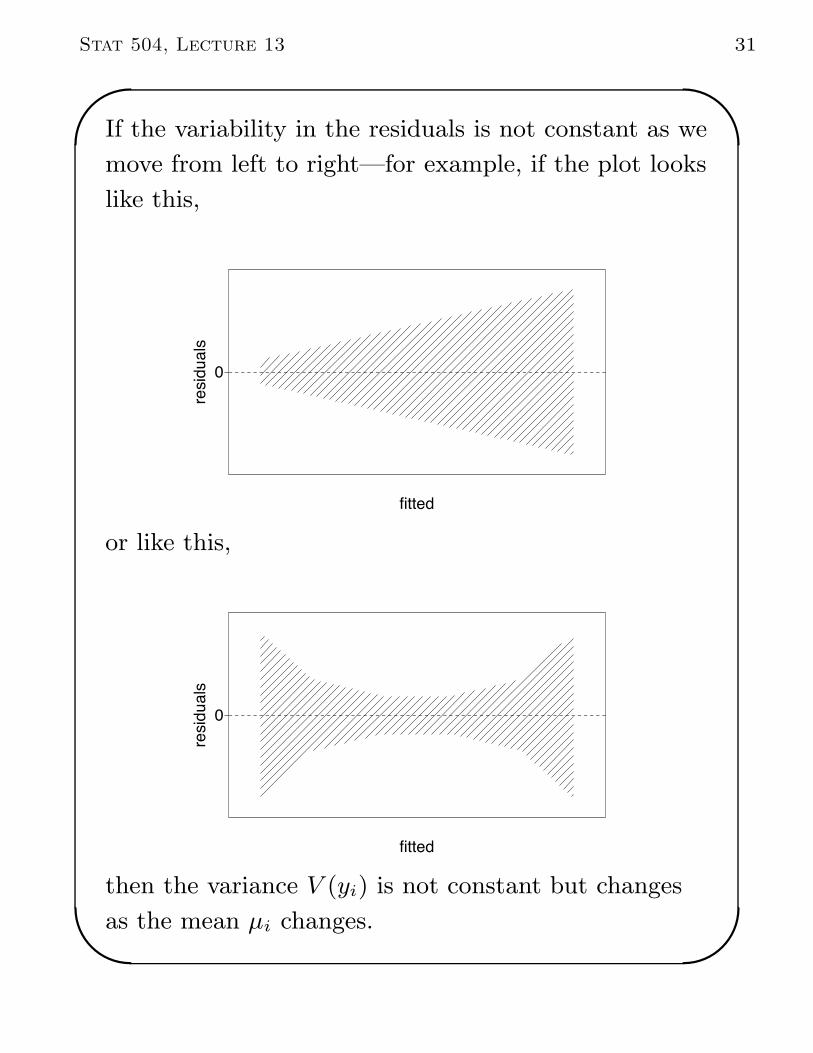
If the variability in the residuals is not constant as we

move from left to right—for example, if the plot looks

like this,

fitted

resid

uals

0

or like this,

fitted

resid

uals

0

then the variance V (yi) is not constant but changes

as the mean µi changes.


"

#

$

Analogous plots for logistic regression. The

logistic regression model says that the mean of yi is

µi = niπi

where

log

„πi

1 − πi

«= xT

i β,

and that the variance of yi is

V (yi) = niπi(1 − πi).

After fitting the model, we can calculate the Pearson

residuals

ri =yi − µiq

V (yi)=

yi − niπipniπi(1 − πi)

(1)

or the deviance residuals. If the ni’s are “large

enough”, these act something like standardized

residuals in linear regression. To see what’s

happening, we can plot them against the linear

predictors,

ηi = xTi βi,

which are the estimated log-odds of success, for cases

i = 1, . . . , N .


"

#

$

If the logistic regression model were true, we would

expect to see a horizontal band with most of the

residuals falling within ±3:

linear predictor

Pear

son

-3

0

3

If the ni’s become small, then the plot might not have

such a nice pattern, even if the model is true. In the

extreme case of ungrouped data (all ni’s equal to 1),

this plot becomes uninformative. From now on, we’ll

suppose that the ni’s are not too small, so that the

plot is at least somewhat meaningful.

If outliers are present—that is, if a few residuals or

even one residual is substantially larger than

±3—then X2 and G2 may be much larger than the

degrees of freedom. In that situation, the lack of fit

can be attributed to outliers, and the large residuals

will be easy to find in the plot.


"

#

$

Curvature. If the plot of Pearson residuals versus

the linear predictors reveals curvature—for example,

like this,

linear predictor

Pear

son

0

then it suggests that the mean model

log

„πi

1 − πi

«= xT

i β,

has been misspecified in some fashion. That is, it

could be that one or more important covariates do

not influence the log-odds of success in a linear

fashion. For example, it could be that a covariate X

ought to be replaced by a transformation such as√

X

or log X, or by a pair of variables X and X2, etc.


"

#

$

To see whether individual covariates ought to enter in

a the logit model in a non-linear fashion, we could

plot the empirical logits

log

„yi + 1/2

ni − yi + 1/2

«(2)

versus each covariate in the model.

If one of the plots looks substantially non-linear, we

might want to transform that particular covariate.

If many of them are nonlinear, however, it may

suggest that the link function has been

misspecified—i.e., that the left-hand side of (2) should

not involve a logit transformation, but some other

function such as

• log,

• probit (but this is often very close to logit), or

• complementary log-log.

Changing the link function will entirely change the

interpretation of the coefficients; the βj ’s will no

longer be log-odds ratios.


"

#

$

But, depending on what the link function is, they

might still have a nice interpretation. For example, in

a model with a log link, log πi = xTi β, an

exponentiated coefficient exp(βj) becomes a relative

risk.


"

#

$

Test for correctness of the link function.

Hinkley (1985) suggests a nice, easy test to see

whether the link function is plausible:

• Fit the model and save the estimated linear

predictors

ηi = xTi β.

• Add η2i to the model as a new predictor and see if

it’s significant.

A significant result indicates that the link function is

misspecified. A nice feature of this test is that it

applies even to ungrouped data (ni’s equal to one),

for which residual plots are uninformative.

Another test for misspecification of the link function

was proposed by Hosmer and Lemeshow (1989).

Unfortunately, this test has been shown to have very

little power, so we will not discuss it further.


"

#

$

Non-constant variance. Suppose that the residual

plot shows non-constant variance as we move from

left to right:

linear predictor

Pear

son

0

Another way to detect non-constancy of variance is to

plot the absolute values of the residuals versus the

linear predictors and look for a non-zero slope:

linear predictor

abs(

Pear

son)


"

#

$

Non-constant variance in the Pearson residuals means

that the assumed form of the variance function,

V (yi) = niπi(1 − πi),

is wrong and cannot be corrected by simply

introducing a scale factor for overdispersion.

Overdispersion and changes to the variance function

will be discussed later in this course.


"

#

$

Example. The SAS on-line help documentation

provides the following quantal assay dataset. In this

table, xi refers to the log-dose, ni is the number of

subjects exposed, and yi is the number who

responded.

xi yi ni

2.68 10 31

2.76 17 30

2.82 12 31

2.90 7 27

3.02 23 26

3.04 22 30

3.13 29 31

3.20 29 30

3.21 23 30

If we fit a simple logistic regression model, we will

find that the coefficient for xi is highly significant, but

the model doesn’t fit. The plot of Pearson residuals

versus the fitted values resembles a horizontal band,

with no obvious curvature or trends in the variance.

This seems to be a classic example of overdispersion.

We will look at the data next time.

k e y c o n ce p t: b in ary l ogistic r egression w ith...

Documents