K Some Additional Topics

In this chapter we give brief references to supplementary topics and present ideas for possible fur-ther study. The actual work will be left to the reader. The topics are diverse such as historical at-tempts to measure the speed of light, considerations concerning 'natural' units for physical entities, theoretical considerations for calculations of future travel to neighboring fixed stars, the use of al-ternative mathematical formalisms for the STR, representing STR with other diagram types and the difference between measuring and seeing in the STR. Many topics have ended up here – many which I would have gladly dealt with directly but which would have given the book a discouraging length. Furthermore, you should now be very well prepared to tackle these topics independently!

155

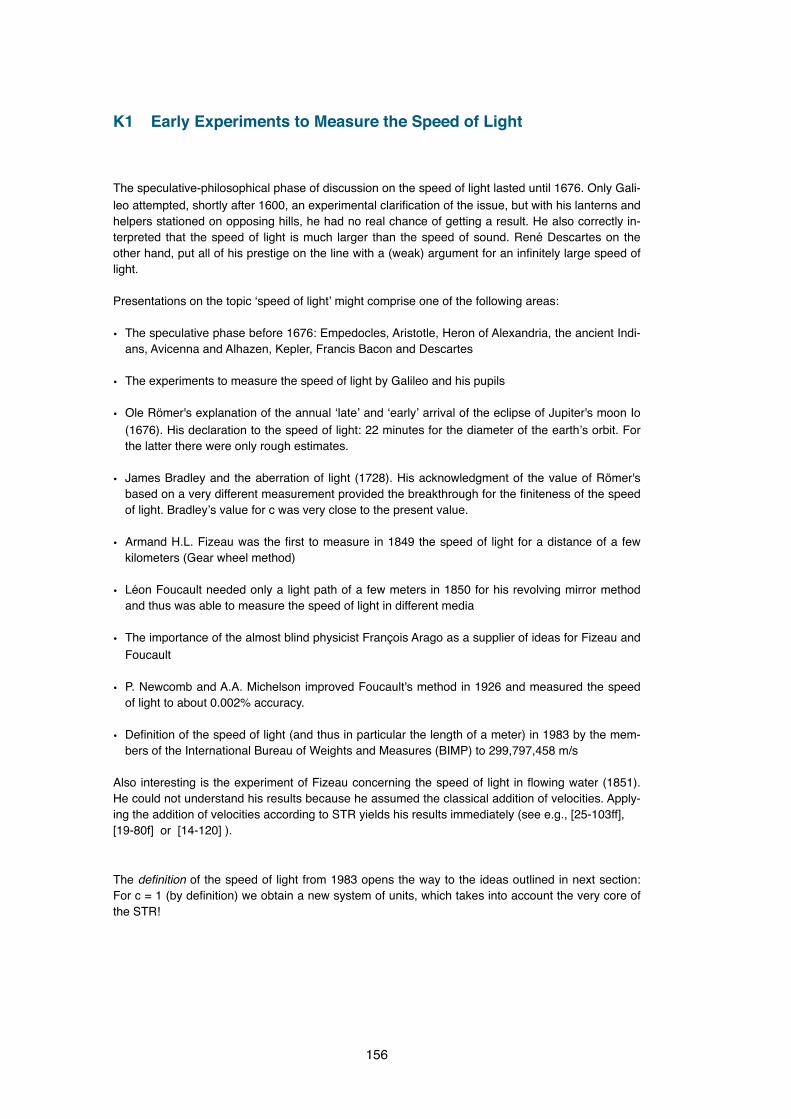
K1 Early Experiments to Measure the Speed of Light

The speculative-philosophical phase of discussion on the speed of light lasted until 1676. Only Gali-leo attempted, shortly after 1600, an experimental clarification of the issue, but with his lanterns and helpers stationed on opposing hills, he had no real chance of getting a result. He also correctly in-terpreted that the speed of light is much larger than the speed of sound. René Descartes on the other hand, put all of his prestige on the line with a (weak) argument for an infinitely large speed of light.

Presentations on the topic ʻspeed of lightʼ might comprise one of the following areas:

• The speculative phase before 1676: Empedocles, Aristotle, Heron of Alexandria, the ancient Indi-ans, Avicenna and Alhazen, Kepler, Francis Bacon and Descartes

• The experiments to measure the speed of light by Galileo and his pupils 

• Ole Römer's explanation of the annual ʻlateʼ and ʻearlyʼ arrival of the eclipse of Jupiter's moon Io (1676). His declaration to the speed of light: 22 minutes for the diameter of the earthʼs orbit. For the latter there were only rough estimates.

• James Bradley and the aberration of light (1728). His acknowledgment of the value of Römer's based on a very different measurement provided the breakthrough for the finiteness of the speed of light. Bradleyʼs value for c was very close to the present value.

• Armand H.L. Fizeau was the first to measure in 1849 the speed of light for a distance of a few kilometers (Gear wheel method) 

• Léon Foucault needed only a light path of a few meters in 1850 for his revolving mirror method and thus was able to measure the speed of light in different media 

• The importance of the almost blind physicist François Arago as a supplier of ideas for Fizeau and Foucault

• P. Newcomb and A.A. Michelson improved Foucault's method in 1926 and measured the speed of light to about 0.002% accuracy. 

• Definition of the speed of light (and thus in particular the length of a meter) in 1983 by the mem-bers of the International Bureau of Weights and Measures (BIMP) to 299,797,458 m/s 

Also interesting is the experiment of Fizeau concerning the speed of light in flowing water (1851). He could not understand his results because he assumed the classical addition of velocities. Apply-ing the addition of velocities according to STR yields his results immediately (see e.g., [25-103ff], [19-80f]  or  [14-120] ).

The definition of the speed of light from 1983 opens the way to the ideas outlined in next section: For c = 1 (by definition) we obtain a new system of units, which takes into account the very core of the STR!

156

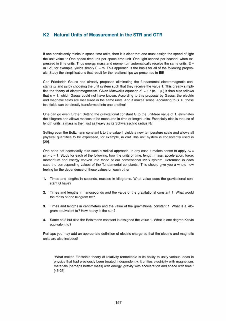
K2 Natural Units of Measurement in the STR and GTR

If one consistently thinks in space-time units, then it is clear that one must assign the speed of light the unit value 1: One space-time unit per space-time unit. One light-second per second, when ex-pressed in time units. Thus energy, mass and momentum automatically receive the same units, E = m • c2, for example, yields simply E = m. This approach is the basis for all of the following propos-als. Study the simplifications that result for the relationships we presented in E5!

Carl Friederich Gauss had already proposed eliminating the fundamental electromagnetic con-stants ε0 and μ0 by choosing the unit system such that they receive the value 1. This greatly simpli-fies the theory of electromagnetism. Given Maxwell's equation c2 = 1 / (ε0 • μ0) it thus also follows that c = 1, which Gauss could not have known. According to this proposal by Gauss, the electric and magnetic fields are measured in the same units. And it makes sense: According to STR, these two fields can be directly transformed into one another!

One can go even further: Setting the gravitational constant G to the unit-free value of 1, eliminates the kilogram and allows masses to be measured in time or length units. Especially nice is the use of length units, a mass is then just as heavy as its Schwarzschild radius RS!

Setting even the Boltzmann constant k to the value 1 yields a new temperature scale and allows all physical quantities to be expressed, for example, in cm! This unit system is consistently used in [29].

One need not necessarily take such a radical approach. In any case it makes sense to apply ε0 = μ0 = c = 1. Study for each of the following, how the units of time, length, mass, acceleration, force, momentum and energy convert into those of our conventional MKS system. Determine in each case the corresponding values of the ʻfundamental constantsʼ. This should give you a whole new feeling for the dependence of these values on each other!

1. Times and lengths in seconds, masses in kilograms. What value does the gravitational con-stant G have? 

2. Times and lengths in nanoseconds and the value of the gravitational constant 1. What would the mass of one kilogram be? 

3. Times and lengths in centimeters and the value of the gravitational constant 1. What is a kilo-gram equivalent to? How heavy is the sun? 

4. Same as 3 but also the Boltzmann constant is assigned the value 1. What is one degree Kelvin equivalent to?

Perhaps you may add an appropriate definition of electric charge so that the electric and magnetic units are also included!

“What makes Einsteinʼs theory of relativity remarkable is its ability to unify various ideas in physics that had previously been treated independently. It unifies electricity with magnetism, materials [perhaps better: mass] with energy, gravity with acceleration and space with time.” [45-25]

157

K3 General Formulas for Velocity Addition, the Doppler Effect and Aberration

In sections D4 and D6 we considered how to add velocities in x direction in the STR. We also de-termined the correct formula for the Doppler Effect when the source moves in a direct line either toward or away from the observer. In Section D5, we saw how ʻtransverseʼ velocities transform and we also derived the angle of aberration one must take into account when the observer moves per-pendicular to the segment connecting the source and observer.

These results are (important) special cases of more general results, which we could easily derive given our previous work. We will forego doing so and simply present references for further reading. Perhaps you may want to find your own derivation?

General formulas for the addition of velocities:

• by Einstein himself: [09-140ff]

• by Horst Melcher: [27-37ff]

• by Michael Fowler: [24-69f]

• by Roman Sexl and Herbert Schmidt: [25-100ff]

• by Jürgen Freund: [26-73ff]

General formulas for the Doppler Effect:

• by Einstein, without calculation: [09-146ff]

• by Horst Melcher: [27-72ff]

• by Jürgen Freund: [26-117ff]

• by Edwin Taylor and John Archibald Wheeler with four-vectors: [11-263]

General formulas for Aberration:

• by Einstein, without calculation: [09-146ff]

• by Horst Melcher: [27-74ff]

• by Jürgen Freund: [26-89ff]

158

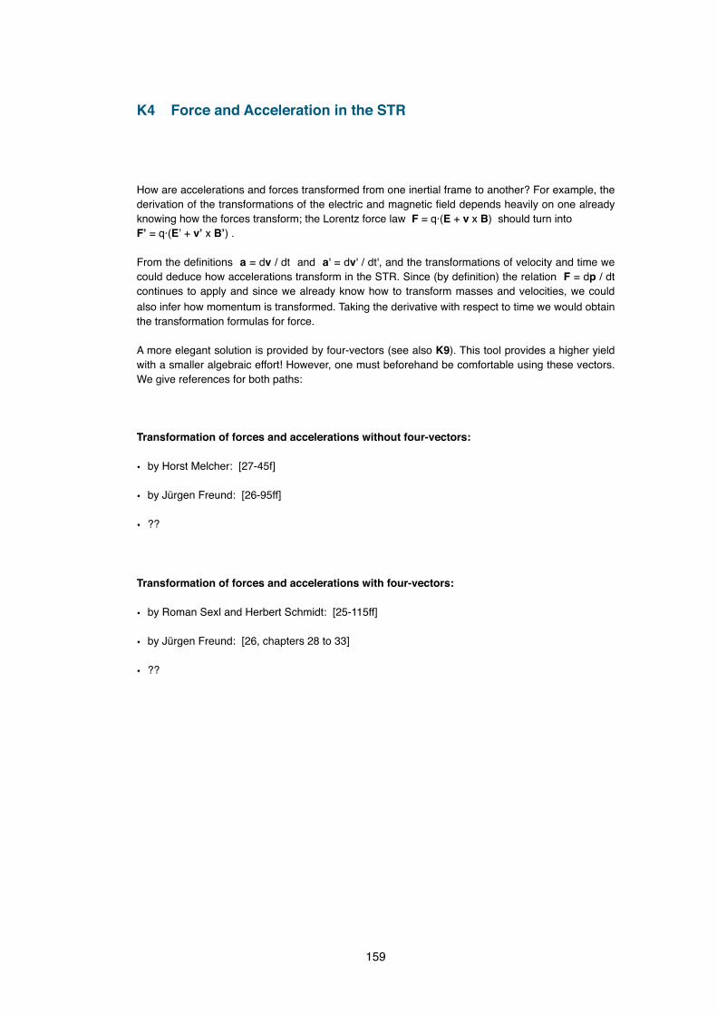
K4 Force and Acceleration in the STR

How are accelerations and forces transformed from one inertial frame to another? For example, the derivation of the transformations of the electric and magnetic field depends heavily on one already knowing how the forces transform; the Lorentz force law F = q·(E + v x B) should turn intoFʼ = q·(Eʼ + vʼ x Bʼ) .

From the definitions  a = dv / dt  and  a' = dv' / dt', and the transformations of velocity and time we could deduce how accelerations transform in the STR. Since (by definition) the relation  F = dp / dt  continues to apply and since we already know how to transform masses and velocities, we could also infer how momentum is transformed. Taking the derivative with respect to time we would obtain the transformation formulas for force.

A more elegant solution is provided by four-vectors (see also K9). This tool provides a higher yield with a smaller algebraic effort! However, one must beforehand be comfortable using these vectors. We give references for both paths:

Transformation of forces and accelerations without four-vectors:

• by Horst Melcher: [27-45f]

• by Jürgen Freund: [26-95ff]

• ??

Transformation of forces and accelerations with four-vectors:

• by Roman Sexl and Herbert Schmidt: [25-115ff]

• by Jürgen Freund: [26, chapters 28 to 33]

• ??

159

K5 The "Conquest of Space"

It is a nice exercise in mathematics and physics to calculate a human voyage to a nearby star. Hu-man, here, means that during the acceleration at the start and during the deceleration before the return the passengers should feel a constant acceleration equivalent to the gravitational force felt on the surface of the earth. Given the desired cruise velocity after the acceleration phase and the distance to the destination then one has all of the information needed.

Kranzer investigates in [43] such a trip to the nearest star α Centauri (distance about 4.2 light years) at a speed of 0.9 • c after the acceleration phase. He uses a few formulas without showing their derivation. For interested students this is a nice challenge! Calculus at the high school level is sufficient to do the calculations. The starting point is the following equation (see also section E4!)

After division by m0 one obtains for the speed of the space vehicle, the following differential equa-tion

Students can at least verify that the following functions for v(t) and x(t) satisfy this differential equa-tion:

The space travelerʼs elapsed proper time during the acceleration phase is then calculated by taking into account that the following always applies

Forming the integral on the right side for the duration of the acceleration phase in coordinate time t for an observer on the earth, yields the elapsed proper time Δτ for a passenger in the spaceship. The result is (for v0 = 0 and x0 = 0)

The journey there and back takes around 12 years for the earth-bound people, while more than three and a half years elapse on-board. How to achieve technically a cruise velocity of 0.9 • c for three-quarters the start mass (!) remains an unsolved miracle. To speak of an impending "conquest of space" is extremely exaggerated.

For people who like to do calculations, [27] contains a lot of stimulating material on pages 164 to 230!  Also [25-161ff] discusses what the STR has to say about travel in our cosmic neighborhood.

160

€

Δτ = cg⋅ ln t + c2

g2 + t2

t 0

t1

€

mo ⋅g = konstant = dpdt

= dpdv

⋅dvdt

= mo ⋅ddv

v

1− v2

c2

⋅dvdt

= mo ⋅ 1− v2

c2

−32⋅dvdt

€

g ⋅ 1− v2

c2

32

= dvdt

€

v(t) = v0 + g ⋅c ⋅ tc2 + g2 ⋅ t2

; x(t) = x0 + v0 ⋅ t + c2

g⋅ 1+

g2 ⋅ t2

c2 −1

€

dτ = 1− v2

c2 ⋅dt

K6 Alternative Derivation of E = m·c2

We derived this formula in E4 in the usual way using kinetic energy and the amount of work in-vested in the acceleration of the mass. Similar to the Pythagorean Theorem, however, there are many proofs and derivations of this famous equation. I have already alluded to probably the most beautiful in the last paragraph of section E5. In this case Einstein used the conservation of momen-tum and the conservation of energy as well as the formulas for the energy and the momentum of photons. It is presented in [22-98ff].

Some other nice proofs (see [26-55ff], [15-131ff]) also use the momentum of light particles or the radiation pressure exerted by electromagnetic wave activity. This quantity was known in 1880 (i.e., ʻlongʼ before quantum theory) from the theory of Maxwell.

Max Born chose a different approach to represent Einstein's relativity theories in his book [42] for the general public first published in 1920. He derives the formula from the inelastic collision of two clumps moving at non-relativistic velocities, i.e., exactly as shown in E3. This method is, in princi-ple, the same used by Sexl et al. in [11-24]: The formula for the increase in mass after its having been accelerated is expanded as a power series, whose fourth and higher order terms of v/c are dropped, thereby yielding Ekin = Δm • c2.

Einstein used a similar approach in September 1905. In his essay entitled "Does the Inertia of a Body Depend on Its Energy Content?" he derives the famous equation from his transformation for-mulas for radiation energy, which we have not discussed. The essay is only four pages, but it can not be recommended for general reading. However, we can understand the last sections, in which Einstein shows that he is quite aware of the general implications of his formula. In the quote below, we have replaced the character L, which Einstein still used at that time for energy, with E and for the speed of light we have written c instead of V:

“If a body emits the energy E in the form of radiation, its mass decreases by E/c2. Here it is obviously inessential that the energy taken from the body turns into radiant energy, so we are led to the more general conclusion:The mass of a body is a measure of its energy content; if the energy changes by E, the mass changes in the same sense by E/(9 • 1020) if the energy is measured in ergs and the mass in grams.It is not excluded that it will prove possible to test this theory using bodies whose energy content is variable to a high degree (e.g., radium salts).If the theory agrees with the facts, then radiation carries inertia between emitting and ab-sorbing bodies.”

Bern, September 1905.         [09-164]

Original publication in "Annalen der Physik", vol. 18 [1905], p.639-641. All of the works of Einstein in the journal "Annalen der Physik" can be downloaded as pdf photocopies athttp://www.physik.uni-augsburg.de/annalen/history/Einstein-in-AdP.htm

161

K7 Deriving the Formula for Addition of Speeds from an Epstein Diagram

In D3, we promised a proof of the formula (red box in D4) for the relativistic addition of speeds based directly on Epstein diagrams and not using the Lorentz transformations. Basis for this is a drawing by Epstein himself in Appendix A of the second edition of [15].  We have redrawn Epstein's figure in a way to best support our proof:

On the left one sees the Epstein diagram for the following situation: Blue moves with velocity w' in the reference system of Red, and thus sin(β) = w' / c. The proper length of the distance traveled is AB, and the trip takes time AF for Blue, while Red measures time AG = AK.

On the right you see that Red moves relative to Black, and thus, as usual, sin(α) = v / c. Also for Black Blue moves from the start to the end of the segment CD: If Blue reaches I, the endpoint D of the segment is in O and therefore they coincide for Black spatially in E. The time intervals that Red and Blue measure are unchanged (CM = AK and CH = AF, respectively), and also the proper length of Blue's path from the viewpoint of Red is unchanged (AB = CD = QO).

The formula for addition of speeds is proved if we can show

€

sin(γ) = sin(α) + sin(β)1 + sin(α) ⋅sin(β)

162

We do not need all of the following segments. Of course, their physical meaning is also irrelevant for the proof. However:

AK = AG = BL = CM = EO time elapsed for RedAB = FG = KL = CD = QO length of Blue's path for Rd, proper length of this pathAF = BG = CH = EI time elapsed for BlueCE = HI = MO length of Blue's path for blackCI = CQ = CP time elapsed for Black

The calculation is then quite simple:

The interpretation of this calculation is left to the reader: If one assumes that we have already proven the formula for addition of speeds, then these calculations should check the correctness of the above construction of the angle γ. If one accepts the correctness of the above drawing, then the calculation gives a proof for the addition of speeds, independent of the Lorentz transformations!

It requires some experience dealing with Epstein diagrams to recognize the correctness of the con-struction free of doubt. So it is perhaps not the didactic approach of first choice. Nevertheless, the drawing of Epstein shows clearly some of the most important aspects: Since the proper time of the sequence for Blue is an invariant (AF = BG = CH = EI), then the addition of two velocities each smaller than c, will always yield a speed which is itself also smaller than c. If Blue moves horizon-tally with respect to Red (i.e., such as light with velocity c), then Blue will also move horizontally with respect to Black: v ⊕ c = c .

I would like to reiterate my thanks to Alfred Hepp for drawing my attention in the first place to ap-pendix A in the second edition of [15]. He also persistently encouraged me to expand the construc-tion of Epstein into a proof of the addition of speeds formula based solely on Epstein diagrams. Dissatisfied with my first proof, he also made significant contributions resulting in the present, much simpler derivation.

Another suggestion: The ⊕-addition makes the open interval (-1, 1) a commutative group. The identity element is zero and the inverse of v is -v. The addition is also monotonic in the sense that if a < b then it follows that a ⊕ d  <  b ⊕ d. Prove twice that ⊕-addition is associative: a) by formal algebraic calculation  and  b) by physical interpretation. Why must the two endpoints 1 and -1 be excluded?

163

€

sin(γ) = CECI

= MOCQ

= MN +NOCN+NQ

= CM ⋅ tan(α) + QO/ cos(α)CM / cos(α) + QO ⋅ tan(α)

=

= AG ⋅ tan(α) + AB/ cos(α)AG/ cos(α) + AB ⋅ tan(α)

= AG ⋅ tan(α) + AG ⋅sin(β) / cos(α)AG/ cos(α) + AG ⋅sin(β) ⋅ tan(α)

=

= tan(α) + sin(β) / cos(α)1/ cos(α) + sin(β) ⋅ tan(α)

= sin(α) + sin(β)1+ sin(β) ⋅sin(α)

= sin(α) + sin(β)1+ sin(α) ⋅sin(β)

K8 The Transformation of Electromagnetic Quantities

We should again emphasize that our representation of the STR is incomplete: The implications for electricity and magnetism are not discussed, although the impetus for the development of this as-pect of the STR came from this corner. Once again I refer (see F6) to the work on this subject by other authors.

STR and Electromagnetism in elementary presentation

• by Michael Fowler [24]

• ??

• ??

STR and Electromagnetism with four-vectors

• by Roman Sexl and Herbert Schmidt [25-177ff]

• by Jürgen Freund [26, chapter 34]

• ??

STR and Electromagnetism with vector analysis

• by Albert EInstein [09-142ff]

• ??

• in any university level text book

164

K9 SRT with Four-Vectors

Geometric problems can be treated with many different mathematical techniques. For example, you can calculate the volume of a tetrahedron using basic geometry, using vector geometry or using integral calculus. Certain questions can often be elegantly answered through the appropriate ap-proach, while another approach would be complicated or provide only approximate success.

The best methodology for doing algebraic calculations in the STR is the one with four-vectors! Not only the place and time of an event, but also all other physical quantities are consistently described by vectors with 4 components: There are the four-speed, four-acceleration, the four-force, the four-momentum and the four-current vectors. All of these four-vectors transform themselves according to the Lorentz transformations in the transition to another coordinate system, just as we have seen with location and time coordinates. And for any four-vectors A and B, there is a simple scalar prod-uct A • B which yields a constant value, independent of the reference system!

Let us take as examples the four-momentum P and the four-speed V:

P = ( Etot/c, px, py, pz ) = mo/√ ·( c , vx, vy, vz ) = mo·V or as shorthand

P = ( Etot/c, p ) = mo/√ ·(c, v) = mo·V

Where p is the 3d-momentum vektor and v the 3d-velocity vector. The scalar product of two four-vectors (x0, x1, x2, x3) and (y0, y1, y2, y3) is defined by x0·y0 – x1·y1 – x2·y2 – x3·y3 . Quickly computing P2 and V2 using this definition of the square of a vector shows:

P2 = (Etot/c)2 – p2 = (Etot2 – p2·c2)/c2 = Eo2 /c2 = mo2 following our equations in E5 !

This is obviously an invariant quantity. Considering the Epstein diagram in E5, if you divide all sides of the right triangle by c, you see that this calculation is just a variant of the Pythagorean Theorem. I would argue that Epstein diagrams and four-vector arithmetic are closely related!

We determine V2 for the case where v = vx and thus vy = 0 = vz :

V2 = (1/√ )2·(c2 – vx2 – 0 – 0) = (c2 – v2)/(1 – v2/c2) = c2·(1 – v2/c2)/(1 – v2/c2) = c2

Again, this is obviously an invariant, i.e., a value independent of the reference system. This result agrees beautifully with Epsteinʼs ʻMyth ʻ! As a small exercise you might consider what P·V means.

The aim of this book was not the algebraic treatment of challenging (and important) examples such as the Compton scattering. Its primary goal was to provide a view on the statements made by the STR and GTR. Or, as Epstein writes: "To understand the Special Theory of Relativity at the gut level, a good myth must be invented" [15-78] . To communicate Epsteinʼs myth was my main con-cern. Once this basis has been attained, it is easy, in a second pass, to acquire some of the techni-cal tools. These tools can then be used to address arbitrarily tricky problems. And the tool for the calculations in special relativity is the algebra of four-vectors.

For an initial study of four-vectors [25] is recommended.  If you work through chapters 12 and 13, you will already have made a significant start. Also, the presentation in [26] is perfectly accessible for someone with a solid high school background. Its title "Special Relativity for Beginners: A Text-book for Undergraduates" describes the level well. The sections on four-vectors in [14] and [19] are restricted to the energy-momentum vector and do not introduce the full power of this concept.

Or take a look at http://www.relativity.li/en/maxwell2/str-maxwell-equations/

165

K10 Measuring and Seeing in the STR

Measuring and seeing are not the same thing. To take a measurement typically means to 'stop' time using a clock at the location of an event, that is, to capture a moment at a given location. Vision is a process by which at a given moment and a specific location we register all of the optical signals, which arrive from various places and which originated at various times. Seeing is therefore compa-rable to photography. In an astronomical photograph of the new moon with an exposure time of 0.1 seconds, we see how it looked about a second ago; the planet Mars, as it was a quarter of an hour ago; and for Saturn we see the light which was reflected about an hour ago! If we increase the ex-posure (a few minutes are sufficient), then perhaps we can even detect a galaxy, revealed by pho-tons which started their journey millions of years ago!

Thus it is possible to see things that no longer exist. A supernova in the Large Magellanic Cloud, a small companion galaxy of our Milky Way, occurred about 163,000 years ago, when we observe it today. The travel-time of the light must also be considered when thinking about how an object ap-pears which is moving very quickly. Consider the following diagram from [25-85]:

Photons leave the corners A and B of the rail car. However, the photons from B cannot reach us.

Only now (after time Δt) are the photons from the front corners C and D sent, which reach our eye simultaneously with those from A.

The car would appear thus if Lorentz contrac-tion did not exist!

We actually see the car thus, since the dis-tance between the corners C and D has shrunk due to the high velocity v.

That is precisely the view of the car we would have, if he had turned away from our line of sight at the angle α, where sin(α) = v / c.

166

The fact that the car appears to have turned away is only due to our 3D interpretation of the 2D image we have of the situation! 

It would be equally correct to say that the car has been tilted and Lorentz contracted. However, we are not used to this interpreta-tion of a visual impression. But it would fit much better to the transformation of the den-sity!Of course, this comment is not from the author of [25].

Meanwhile, there is a group within the physics community, which is using the computing power available today to show how, for example, a flight through the Brandenburg Gate at 0.95 • c would be visually experienced. Sometimes even the change in color due to the optical Doppler effect is taken into account. Clearly, one must play the whole thing back in slow motion, so that it does not run too fast for a human observer. A good location for such visualizations is

www.tempolimit-lichtgeschwindigkeit.de

Ute Kraus of the University of Tübingen is the person behind this address. Her group realized for the Einstein Jubilee of 2005 relativistic bicycle tours through the old towns of Bern and Tübingen. The exhibitions in Ulm and in Bern even offered the visitor to mount a real (stationary) bicycle and pedal away. The pedal speed was then processed by a computer which amplified the effects of 30 km/h to 300,000 km/s. To make it possible to navigate the narrow streets (and still be able to see something!) the houses passed by at the unamplified velocity.

If you delight in such visualizations, then visit the website recommended above. You will also find references and other related material about the theories of relativity of Albert Einstein.

167

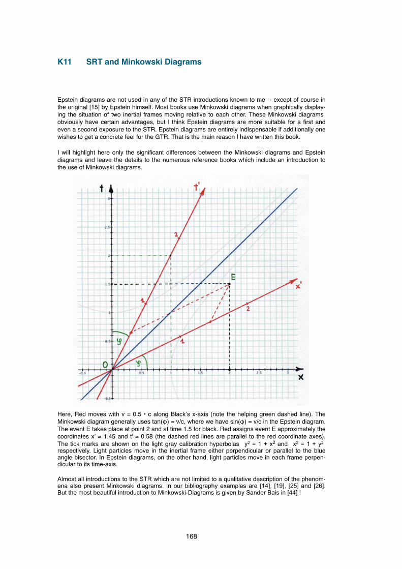
K11 SRT and Minkowski Diagrams

Epstein diagrams are not used in any of the STR introductions known to me   - except of course in the original [15] by Epstein himself. Most books use Minkowski diagrams when graphically display-ing the situation of two inertial frames moving relative to each other. These Minkowski diagrams obviously have certain advantages, but I think Epstein diagrams are more suitable for a first and even a second exposure to the STR. Epstein diagrams are entirely indispensable if additionally one wishes to get a concrete feel for the GTR. That is the main reason I have written this book.

I will highlight here only the significant differences between the Minkowski diagrams and Epstein diagrams and leave the details to the numerous reference books which include an introduction to the use of Minkowski diagrams.

Here, Red moves with v = 0.5 • c along Blackʼs x-axis (note the helping green dashed line). The Minkowski diagram generally uses tan(φ) = v/c, where we have sin(φ) = v/c in the Epstein diagram. The event E takes place at point 2 and at time 1.5 for black. Red assigns event E approximately the coordinates xʼ ≈ 1.45 and t' ≈ 0.58 (the dashed red lines are parallel to the red coordinate axes). The tick marks are shown on the light gray calibration hyperbolas y2 = 1 + x2 and x2 = 1 + y2 respectively. Light particles move in the inertial frame either perpendicular or parallel to the blue angle bisector. In Epstein diagrams, on the other hand, light particles move in each frame perpen-dicular to its time-axis.

Almost all introductions to the STR which are not limited to a qualitative description of the phenom-ena also present Minkowski diagrams. In our bibliography examples are [14], [19], [25] and [26]. But the most beautiful introduction to Minkowski-Diagrams is given by Sander Bais in [44] !

168

K12 SRT and Penrose Diagrams

There are many other possibilities to graphically represent relativistic relationships. The two British mathematicians B. Carter and R. Penrose have a model in which the infinitely extended Minkowski plane is projected onto a square in which light beams continue to be straight lines running parallel to one of the two angle bisectors. Lines of constant time or constant location become hyperbolas. In the center of the picture one sees the undistorted current local event, while distant events are com-pressed together:

This figure is taken from the free encyclopedia Wikipedia. On the website of Franz Embacher

http://homepage.univie.ac.at/Franz.Embacher/Rel/

you can find a Java applet, which allows you to play with this coordinate transformation. If you play with it seriously and use it to solve the problems that are suggested, then you gain a good under-standing of what this model offers.

The arc tangent is used since it is a monotonically increasing function; approximates the identity function in the vicinity of the origin (i.e., f (x) ≈ x); and has a finite limit as x approaches ∞. Thus the corners of the square lie ± π / 2 from the origin. The mapping of the Minkowski plane into the Penrose-world is defined by the following equations:

xʼ + tʼ = ArcTan (x + t) and xʼ – tʼ = ArcTan (x – t)

Addition (and subtraction) of these equations immediately gives the transformation equations for xʼ and tʼ respectively. It is easy to show that light beams that go out from the origin in the Penrose diagram are angle bisectors. Show that all the light beams run parallel to these!

Also: Find a model yourself, which has similar properties! Is the arc tangent really better than your model?

169

K13 SRT and Asano Diagrams

After ʻcompletingʼ this book I discovered in the basement of the Central Library in Zurich a little book [45], in which the two brothers Seiichi and Shiro Asano present their "Space-Time Circular Diagrams". The first Japanese edition was published in 1983, thus coinciding with the first edition [15] by Epstein! The brothers Asano, as small boys, were impressed by all of the whoopla of Ein-stein's visit to Japan in 1922. They went on to have careers as an electrical engineer and a physi-cian, respectively. After retiring, they decided to elucidate the STR for themselves and others.

Like Epstein they take as their starting point Minkowskiʼs equation ∆τ2 = c·∆t2 – ∆x2 – ∆y2 – ∆z2 (times and lengths are measured in the same units), suppress the y and z component and rear-range the remainder of the relationship ∆τ2 = c·∆t2 – ∆x2 so that it can be interpreted as the equa-tion of a circle: c·∆t2 = ∆τ2 + ∆x2 . Also with the Asano brothers the straight line on which B moves with constant velocity v through space-time is tilted with respect to the time-axis of a stationary ob-server A by an angle φ, where sin(φ) = v / c. On [45-49] they consider right triangles that are con-gruent to those in the corresponding diagrams of Epstein.

A and B have met at O and both have set their clocks to zero. The sine of the angle AOB is v/c. At B1, B2 and B3, we have right angles according to the theorem of Thales.

When the time t3 has elapsed for A, which corre-sponds to the distance OA3, then for B the time which corresponds to the distance OB3 has elapsed. At time t3, B is the distance X3 = A3B3 from A.

We obtain the corresponding congruent right tri-angles of the Epstein diagram by reflecting those of the Asano diagram through the angle bisector of AOB.

170

Also the Epstein diagrams characteristic semicircles around O occasionally appear in the Asano diagrams; however, they indicate only the elapsed time intervals for A. The diagrams show a dila-tion with center O and a stretching factor, which is proportional to time [45-50]:

But for the spatial axes the brothers have no good solution. One might say that they still tried to separate time, space-time and space. The dashed curves, which indicate at what speed a certain distance (in light-seconds) is reached, are quite complicated:

Do you notice the point which belong to the Pythagorean triple (6/8/10) and which also lies on the straight line for v = 0.6 • c?

Epstein diagrams are clearly preferable to those of Asano. They are based on a simple postulate and they are more easily drawn and read. But it is interesting to note that similar approaches ap-peared in different places simultaneously. The Asano brothers do not mention their ʻcompetitorʼ Epstein in the first English edition of 1994.

171