· 4 contents 2.29 system . . . . . . . . . . . . . . . . . . . . . . . . . . . . . . . . . . . ....
TRANSCRIPT

SPEX User’s Manual
Jelle Kaastra
Rolf Mewe & Ton Raassen
Version 2.0
October 29, 2009

2

Contents
1 Introduction 7
1.1 Preface . . . . . . . . . . . . . . . . . . . . . . . . . . . . . . . . . . . . . . . . . 7
1.2 Sectors and regions . . . . . . . . . . . . . . . . . . . . . . . . . . . . . . . . . . . 7
1.2.1 Introduction . . . . . . . . . . . . . . . . . . . . . . . . . . . . . . . . . . 7
1.2.2 Sky sectors . . . . . . . . . . . . . . . . . . . . . . . . . . . . . . . . . . . 8
1.2.3 Detector regions . . . . . . . . . . . . . . . . . . . . . . . . . . . . . . . . 8
1.3 Different types of spectral components . . . . . . . . . . . . . . . . . . . . . . . . 8
2 Syntax overview 11
2.1 Abundance: standard abundances . . . . . . . . . . . . . . . . . . . . . . . . . . 11
2.2 Ascdump: ascii output of plasma properties . . . . . . . . . . . . . . . . . . . . . 13
2.3 Bin: rebin the spectrum . . . . . . . . . . . . . . . . . . . . . . . . . . . . . . . . 15
2.4 Calculate: evaluate the spectrum . . . . . . . . . . . . . . . . . . . . . . . . . . . 15
2.5 Comp: create, delete and relate spectral components . . . . . . . . . . . . . . . . 16
2.6 Data: read response file and spectrum . . . . . . . . . . . . . . . . . . . . . . . . 17
2.7 DEM: differential emission measure analysis . . . . . . . . . . . . . . . . . . . . 18
2.8 Distance: set the source distance . . . . . . . . . . . . . . . . . . . . . . . . . . . 20
2.9 Egrid: define model energy grids . . . . . . . . . . . . . . . . . . . . . . . . . . . 22
2.10 Elim: set flux energy limits . . . . . . . . . . . . . . . . . . . . . . . . . . . . . . 23
2.11 Error: Calculate the errors of the fitted parameters . . . . . . . . . . . . . . . . . 24
2.12 Fit: spectral fitting . . . . . . . . . . . . . . . . . . . . . . . . . . . . . . . . . . . 25
2.13 Ibal: set type of ionisation balance . . . . . . . . . . . . . . . . . . . . . . . . . . 26
2.14 Ignore: ignoring part of the spectrum . . . . . . . . . . . . . . . . . . . . . . . . 27
2.15 Ion: select ions for the plasma models . . . . . . . . . . . . . . . . . . . . . . . . 27
2.16 Log: Making and using command files . . . . . . . . . . . . . . . . . . . . . . . . 28
2.17 Menu: Menu settings . . . . . . . . . . . . . . . . . . . . . . . . . . . . . . . . . . 29
2.18 Model: show the current spectral model . . . . . . . . . . . . . . . . . . . . . . . 30
2.19 Multiply: scaling of the response matrix . . . . . . . . . . . . . . . . . . . . . . . 30
2.20 Obin: optimal rebinning of the data . . . . . . . . . . . . . . . . . . . . . . . . . 31
2.21 Par: Input and output of model parameters . . . . . . . . . . . . . . . . . . . . . 31
2.22 Plot: Plotting data and models . . . . . . . . . . . . . . . . . . . . . . . . . . . . 34
2.23 Quit: finish the program . . . . . . . . . . . . . . . . . . . . . . . . . . . . . . . . 38
2.24 Sector: creating, copying and deleting of a sector . . . . . . . . . . . . . . . . . . 38
2.25 Shiftplot: shift the plotted spectrum for display purposes . . . . . . . . . . . . . 39
2.26 Simulate: Simulation of data . . . . . . . . . . . . . . . . . . . . . . . . . . . . . 40
2.27 Step: Grid search for spectral fits . . . . . . . . . . . . . . . . . . . . . . . . . . . 41
2.28 Syserr: systematic errors . . . . . . . . . . . . . . . . . . . . . . . . . . . . . . . . 42

4 CONTENTS
2.29 System . . . . . . . . . . . . . . . . . . . . . . . . . . . . . . . . . . . . . . . . . . 43
2.30 Use: reuse part of the spectrum . . . . . . . . . . . . . . . . . . . . . . . . . . . . 432.31 Var: various settings for the plasma models . . . . . . . . . . . . . . . . . . . . . 44
2.31.1 Overview . . . . . . . . . . . . . . . . . . . . . . . . . . . . . . . . . . . . 44
2.31.2 Syntax . . . . . . . . . . . . . . . . . . . . . . . . . . . . . . . . . . . . . . 452.31.3 Examples . . . . . . . . . . . . . . . . . . . . . . . . . . . . . . . . . . . . 45
2.32 Vbin: variable rebinning of the data . . . . . . . . . . . . . . . . . . . . . . . . . 452.33 Watch . . . . . . . . . . . . . . . . . . . . . . . . . . . . . . . . . . . . . . . . . . 46
3 Spectral Models 493.1 Overview of spectral components . . . . . . . . . . . . . . . . . . . . . . . . . . . 493.2 Absm: Morrison & McCammon absorption model . . . . . . . . . . . . . . . . . . 49
3.3 Bb: Blackbody model . . . . . . . . . . . . . . . . . . . . . . . . . . . . . . . . . 493.4 Cf: isobaric cooling flow differential emission measure model . . . . . . . . . . . . 513.5 Cie: collisional ionisation equilibrium model . . . . . . . . . . . . . . . . . . . . . 51
3.5.1 Temperatures . . . . . . . . . . . . . . . . . . . . . . . . . . . . . . . . . . 513.5.2 Line broadening . . . . . . . . . . . . . . . . . . . . . . . . . . . . . . . . 523.5.3 Density effects . . . . . . . . . . . . . . . . . . . . . . . . . . . . . . . . . 52
3.5.4 Non-thermal electron distributions . . . . . . . . . . . . . . . . . . . . . . 523.5.5 Abundances . . . . . . . . . . . . . . . . . . . . . . . . . . . . . . . . . . . 52
3.5.6 Parameter description . . . . . . . . . . . . . . . . . . . . . . . . . . . . . 533.6 Comt: Comptonisation model . . . . . . . . . . . . . . . . . . . . . . . . . . . . . 54
3.6.1 Some modifications . . . . . . . . . . . . . . . . . . . . . . . . . . . . . . . 54
3.7 Dbb: Disk blackbody model . . . . . . . . . . . . . . . . . . . . . . . . . . . . . . 543.8 Delt: delta line model . . . . . . . . . . . . . . . . . . . . . . . . . . . . . . . . . 553.9 Dem: Differential Emission Measure model . . . . . . . . . . . . . . . . . . . . . 56
3.10 Dust: dust scattering model . . . . . . . . . . . . . . . . . . . . . . . . . . . . . . 563.11 Etau: simple transmission model . . . . . . . . . . . . . . . . . . . . . . . . . . . 57
3.12 Euve: EUVE absorption model . . . . . . . . . . . . . . . . . . . . . . . . . . . . 573.13 File: model read from a file . . . . . . . . . . . . . . . . . . . . . . . . . . . . . . 583.14 Gaus: Gaussian line model . . . . . . . . . . . . . . . . . . . . . . . . . . . . . . 58
3.15 Hot: collisional ionisation equilibrium absorption model . . . . . . . . . . . . . . 593.16 Knak: segmented power law transmission model . . . . . . . . . . . . . . . . . . 593.17 Laor: Relativistic line broadening model . . . . . . . . . . . . . . . . . . . . . . . 60
3.18 Lpro: Spatial broadening model . . . . . . . . . . . . . . . . . . . . . . . . . . . . 603.19 Mbb: Modified blackbody model . . . . . . . . . . . . . . . . . . . . . . . . . . . 61
3.20 Neij: Non-Equilibrium Ionisation Jump model . . . . . . . . . . . . . . . . . . . . 623.21 Pdem: DEM models . . . . . . . . . . . . . . . . . . . . . . . . . . . . . . . . . . 62
3.21.1 Short description . . . . . . . . . . . . . . . . . . . . . . . . . . . . . . . . 62
3.22 Pow: Power law model . . . . . . . . . . . . . . . . . . . . . . . . . . . . . . . . . 633.23 Reds: redshift model . . . . . . . . . . . . . . . . . . . . . . . . . . . . . . . . . . 643.24 Refl: Reflection model . . . . . . . . . . . . . . . . . . . . . . . . . . . . . . . . . 65
3.25 Rrc: Radiative Recombination Continuum model . . . . . . . . . . . . . . . . . . 653.26 Slab: thin slab absorption model . . . . . . . . . . . . . . . . . . . . . . . . . . . 66
3.27 Spln: spline continuum model . . . . . . . . . . . . . . . . . . . . . . . . . . . . . 673.28 Vblo: Rectangular velocity broadening model . . . . . . . . . . . . . . . . . . . . 683.29 Vgau: Gaussian velocity broadening model . . . . . . . . . . . . . . . . . . . . . 68
3.30 Vpro: Velocity profile broadening model . . . . . . . . . . . . . . . . . . . . . . . 69

CONTENTS 5
3.31 Warm: continuous photoionised absorption model . . . . . . . . . . . . . . . . . . 69
3.32 Wdem: power law differential emission measure model . . . . . . . . . . . . . . . 70
3.33 xabs: photoionised absorption model . . . . . . . . . . . . . . . . . . . . . . . . . 71
4 More about spectral models 73
4.1 Absorption models . . . . . . . . . . . . . . . . . . . . . . . . . . . . . . . . . . . 73
4.1.1 Introduction . . . . . . . . . . . . . . . . . . . . . . . . . . . . . . . . . . 73
4.1.2 Thomson scattering . . . . . . . . . . . . . . . . . . . . . . . . . . . . . . 73
4.1.3 Different types of absorption models . . . . . . . . . . . . . . . . . . . . . 73
4.1.4 Dynamical model for the absorbers . . . . . . . . . . . . . . . . . . . . . . 74
4.2 Atomic database for the absorbers . . . . . . . . . . . . . . . . . . . . . . . . . . 75
4.2.1 K-shell transitions . . . . . . . . . . . . . . . . . . . . . . . . . . . . . . . 75
4.2.2 L-shell transitions . . . . . . . . . . . . . . . . . . . . . . . . . . . . . . . 76
4.2.3 M-shell transitions . . . . . . . . . . . . . . . . . . . . . . . . . . . . . . . 77
4.3 Non-equilibrium ionisation (NEI) calculations . . . . . . . . . . . . . . . . . . . . 77
4.4 Non-thermal electron distributions . . . . . . . . . . . . . . . . . . . . . . . . . . 77
4.5 Supernova remnant (SNR) models . . . . . . . . . . . . . . . . . . . . . . . . . . 78
5 More about plotting 81
5.1 Plot devices . . . . . . . . . . . . . . . . . . . . . . . . . . . . . . . . . . . . . . . 81
5.2 Plot types . . . . . . . . . . . . . . . . . . . . . . . . . . . . . . . . . . . . . . . . 81
5.3 Plot colours . . . . . . . . . . . . . . . . . . . . . . . . . . . . . . . . . . . . . . . 82
5.4 Plot line types . . . . . . . . . . . . . . . . . . . . . . . . . . . . . . . . . . . . . 84
5.5 Plot text . . . . . . . . . . . . . . . . . . . . . . . . . . . . . . . . . . . . . . . . . 85
5.5.1 Font types (font) . . . . . . . . . . . . . . . . . . . . . . . . . . . . . . . . 85
5.5.2 Font heights (fh) . . . . . . . . . . . . . . . . . . . . . . . . . . . . . . . . 86
5.5.3 Special characters . . . . . . . . . . . . . . . . . . . . . . . . . . . . . . . 86
5.6 Plot captions . . . . . . . . . . . . . . . . . . . . . . . . . . . . . . . . . . . . . . 88
5.7 Plot symbols . . . . . . . . . . . . . . . . . . . . . . . . . . . . . . . . . . . . . . 89
5.8 Plot axis units and scales . . . . . . . . . . . . . . . . . . . . . . . . . . . . . . . 90
5.8.1 Plot axis units . . . . . . . . . . . . . . . . . . . . . . . . . . . . . . . . . 90
5.8.2 Plot axis scales . . . . . . . . . . . . . . . . . . . . . . . . . . . . . . . . . 90
6 Auxilary programs 95
6.1 Trafo . . . . . . . . . . . . . . . . . . . . . . . . . . . . . . . . . . . . . . . . . . . 95
6.1.1 File formats spectra . . . . . . . . . . . . . . . . . . . . . . . . . . . . . . 95
6.1.2 File formats responses . . . . . . . . . . . . . . . . . . . . . . . . . . . . . 97
6.1.3 Multiple spectra . . . . . . . . . . . . . . . . . . . . . . . . . . . . . . . . 98
6.1.4 How to use trafo . . . . . . . . . . . . . . . . . . . . . . . . . . . . . . . . 98
7 Response matrices 99
7.1 Respons matrices . . . . . . . . . . . . . . . . . . . . . . . . . . . . . . . . . . . . 99
7.2 Introduction . . . . . . . . . . . . . . . . . . . . . . . . . . . . . . . . . . . . . . . 99
7.3 Data binning . . . . . . . . . . . . . . . . . . . . . . . . . . . . . . . . . . . . . . 100
7.3.1 Introduction . . . . . . . . . . . . . . . . . . . . . . . . . . . . . . . . . . 100
7.3.2 The Shannon theorem . . . . . . . . . . . . . . . . . . . . . . . . . . . . . 100
7.3.3 Integration of Shannon’s theorem . . . . . . . . . . . . . . . . . . . . . . . 101
7.3.4 The χ2 test . . . . . . . . . . . . . . . . . . . . . . . . . . . . . . . . . . . 102

6 CONTENTS
7.3.5 Extension to complex spectra . . . . . . . . . . . . . . . . . . . . . . . . . 1047.3.6 Difficulties with the χ2 test . . . . . . . . . . . . . . . . . . . . . . . . . . 1057.3.7 The Kolmogorov-Smirnov test . . . . . . . . . . . . . . . . . . . . . . . . 1067.3.8 Examples . . . . . . . . . . . . . . . . . . . . . . . . . . . . . . . . . . . . 1087.3.9 Final remarks . . . . . . . . . . . . . . . . . . . . . . . . . . . . . . . . . . 110
7.4 Model binning . . . . . . . . . . . . . . . . . . . . . . . . . . . . . . . . . . . . . 1117.4.1 Model energy grid . . . . . . . . . . . . . . . . . . . . . . . . . . . . . . . 1117.4.2 Evaluation of the model spectrum . . . . . . . . . . . . . . . . . . . . . . 1127.4.3 Binning the model spectrum . . . . . . . . . . . . . . . . . . . . . . . . . 1137.4.4 Which approximation to choose? . . . . . . . . . . . . . . . . . . . . . . . 1157.4.5 The effective area . . . . . . . . . . . . . . . . . . . . . . . . . . . . . . . . 1167.4.6 Final remarks . . . . . . . . . . . . . . . . . . . . . . . . . . . . . . . . . . 117
7.5 The proposed response matrix . . . . . . . . . . . . . . . . . . . . . . . . . . . . . 1177.5.1 Dividing the response into components . . . . . . . . . . . . . . . . . . . . 1177.5.2 More complex situations . . . . . . . . . . . . . . . . . . . . . . . . . . . . 1187.5.3 A response component . . . . . . . . . . . . . . . . . . . . . . . . . . . . . 119
7.6 Determining the grids in practice . . . . . . . . . . . . . . . . . . . . . . . . . . . 1217.6.1 Creating the data bins . . . . . . . . . . . . . . . . . . . . . . . . . . . . . 1217.6.2 creating the model bins . . . . . . . . . . . . . . . . . . . . . . . . . . . . 122
7.7 Proposed file formats . . . . . . . . . . . . . . . . . . . . . . . . . . . . . . . . . . 1237.7.1 Proposed response format . . . . . . . . . . . . . . . . . . . . . . . . . . . 1237.7.2 Proposed spectral file format . . . . . . . . . . . . . . . . . . . . . . . . . 125
7.8 examples . . . . . . . . . . . . . . . . . . . . . . . . . . . . . . . . . . . . . . . . 1277.8.1 Introduction . . . . . . . . . . . . . . . . . . . . . . . . . . . . . . . . . . 1277.8.2 Rosat PSPC . . . . . . . . . . . . . . . . . . . . . . . . . . . . . . . . . . 1287.8.3 ASCA SIS0 . . . . . . . . . . . . . . . . . . . . . . . . . . . . . . . . . . . 1287.8.4 XMM RGS data . . . . . . . . . . . . . . . . . . . . . . . . . . . . . . . . 131
7.9 References . . . . . . . . . . . . . . . . . . . . . . . . . . . . . . . . . . . . . . . . 132
8 Installation and testing 1358.1 Testing the software . . . . . . . . . . . . . . . . . . . . . . . . . . . . . . . . . . 135
9 Acknowledgements 1379.1 Acknowledgements . . . . . . . . . . . . . . . . . . . . . . . . . . . . . . . . . . . 137

Chapter 1
Introduction
1.1 Preface
At the time of releasing version 2.0 of the code, the full documentation is not yet available,although major parts have been completed (you are reading that part now). This manual willbe extended during the coming months. Check the version you have (see the front page forthe date it was created). In the mean time, there are several useful hints and documentationavailable at the web site of Alex Blustin (MSSL), who I thank for his help in this. That website can be found at:
http://www.mssl.ucl.ac.uk/ ajb/spex/spex.html
The official SPEX website is:
http://www.sron.nl/divisions/hea/spex/index.html
We apologize for the temporary inconvenience.
1.2 Sectors and regions
1.2.1 Introduction
In many cases an observer analysis the observed spectrum of a single X-ray source. There arehowever situations with more complex geometries.
Example 1: An extended source, where the spectrum may be extracted from different regionsof the detector, but where these spectra need to be analysed simultaneously due to the overlapin point-spread function from one region to the other. This situation is e.g. encountered in theanalysis of cluster data with ASCA or BeppoSAX.
Example 2: For the RGS detector of XMM-Newton, the actual data-space in the dispersiondirection is actually two-dimensional: the position z where a photon lands on the detector andits energy or pulse height E as measured with the CCD detector. X-ray sources that are extendedin the direction of the dispersion axis φ are characterised by spectra that are a function of boththe energy E and off-axis angle φ. The sky photon distribution as a function of (φ,E) is thenmapped onto the (z,E)-plane. By defining appropriate regions in both planes and evaluatingthe correct (overlapping) responses, one may analyse extended sources.
Example 3: One may also fit simultaneously several time-dependent spectra using the sameresponse, e.g. data obtained during a stellar flare.
It is relatively easy to model all these situations (provided that the instrument is understoodsufficiently, of course), as we show below.
8 Introduction
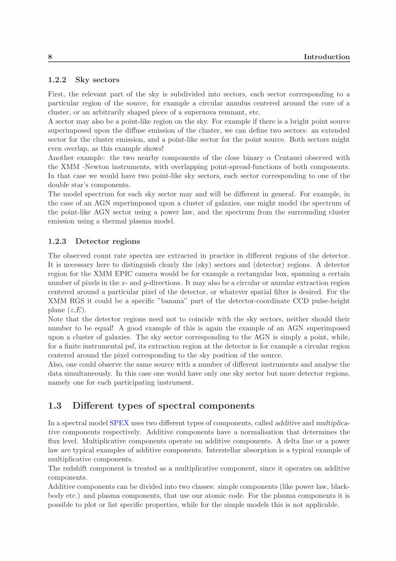
1.2.2 Sky sectors
First, the relevant part of the sky is subdivided into sectors, each sector corresponding to aparticular region of the source, for example a circular annulus centered around the core of acluster, or an arbitrarily shaped piece of a supernova remnant, etc.
A sector may also be a point-like region on the sky. For example if there is a bright point sourcesuperimposed upon the diffuse emission of the cluster, we can define two sectors: an extendedsector for the cluster emission, and a point-like sector for the point source. Both sectors mighteven overlap, as this example shows!
Another example: the two nearby components of the close binary α Centauri observed withthe XMM -Newton instruments, with overlapping point-spread-functions of both components.In that case we would have two point-like sky sectors, each sector corresponding to one of thedouble star’s components.
The model spectrum for each sky sector may and will be different in general. For example, inthe case of an AGN superimposed upon a cluster of galaxies, one might model the spectrum ofthe point-like AGN sector using a power law, and the spectrum from the surrounding clusteremission using a thermal plasma model.
1.2.3 Detector regions
The observed count rate spectra are extracted in practice in different regions of the detector.It is necessary here to distinguish clearly the (sky) sectors and (detector) regions. A detectorregion for the XMM EPIC camera would be for example a rectangular box, spanning a certainnumber of pixels in the x- and y-directions. It may also be a circular or annular extraction regioncentered around a particular pixel of the detector, or whatever spatial filter is desired. For theXMM RGS it could be a specific ”banana” part of the detector-coordinate CCD pulse-heightplane (z,E).
Note that the detector regions need not to coincide with the sky sectors, neither should theirnumber to be equal! A good example of this is again the example of an AGN superimposedupon a cluster of galaxies. The sky sector corresponding to the AGN is simply a point, while,for a finite instrumental psf, its extraction region at the detector is for example a circular regioncentered around the pixel corresponding to the sky position of the source.
Also, one could observe the same source with a number of different instruments and analyse thedata simultaneously. In this case one would have only one sky sector but more detector regions,namely one for each participating instrument.
1.3 Different types of spectral components
In a spectral model SPEX uses two different types of components, called additive and multiplica-tive components respectively. Additive components have a normalisation that determines theflux level. Multiplicative components operate on additive components. A delta line or a powerlaw are typical examples of additive components. Interstellar absorption is a typical example ofmultiplicative components.
The redshift component is treated as a multiplicative component, since it operates on additivecomponents.
Additive components can be divided into two classes: simple components (like power law, black-body etc.) and plasma components, that use our atomic code. For the plasma components it ispossible to plot or list specific properties, while for the simple models this is not applicable.

1.3 Different types of spectral components 9
Multiplicative components can be divided into 3 classes. First, there are the absorption-typecomponents, like interstellar absorption. These components simply are an energy-dependentmultiplication of the original source spectrum. SPEX has both simple absorption componentsas well as absorption components based upon our plasma code. The second class consists ofshifts: redshift (either due to Doppler shifts or due to cosmology) is the prototype of this. Thethird class consists of convolution-type operators. An example is Gaussian velocity broadening.For more information about the currently defined spectral components in SPEX, see chapter 3.

10 Introduction

Chapter 2
Syntax overview
2.1 Abundance: standard abundances
Overview
For the plasm models, a default set of abundances is used. All abundances are calculated rela-tive to those standard values. The current default abundance set is Anders & Grevesse ([1989]).However, it is recommended to use the more recent compilation by Lodders ([2003]). In partic-ular we recommend to use the proto-solar (= solar system) abundances for most applications,as the solar photospheric abundance has been affected by nucleosynthesis (burning of H to He)and settlement in the Sun during its lifetime. The following abundances (Table 2.1) can be usedin SPEX:
Table 2.1: Standard abundance sets
Abbrevation Reference
reset default (=Anders & Grevesse)ag Anders & Grevesse ([1989])allen Allen ([1973])ra Ross & Aller ([1976])grevesse Grevesse et al. ([1992])gs Grevesse & Sauval ([1998])lodders Lodders proto-solar ([2003])solar Lodders solar photospheric ([2003])
For the case of Grevesse & Sauval (1998) we adopted their meteoritic values (in general moreaccurate than the photospheric values, but in most cases consistent), except for He (slightlyenhanced in the solar photosphere due to element migration at the bottom of the convectionzone), C, N and O (largely escaped from meteorites) Ne and Ar (noble gases).In Table 2.2 we show the values of the standard abundances. They are expressed in logarithmicunits, with hydrogen by definition 12.0. For Allen ([1973]) the value for boron is just an upperlimit.
Warning: For Allen ([1973]) the value for boron is just an upper limit.
Syntax
The following syntax rules apply:

12 Syntax overview
Table 2.2: Abundances for the standard sets
Z elem AG Allen RA Grevesse GS Lodders solar
1 H 12.00 12.00 12.00 12.00 12.00 12.00 12.002 He 10.99 10.93 10.80 10.97 10.99 10.98 10.903 Li 1.16 0.70 1.00 1.16 3.31 3.35 3.284 Be 1.15 1.10 1.15 1.15 1.42 1.48 1.415 B 2.6 ¡3.0 2.11 2.6 2.79 2.85 2.786 C 8.56 8.52 8.62 8.55 8.52 8.46 8.397 N 8.05 7.96 7.94 7.97 7.92 7.90 7.838 O 8.93 8.82 8.84 8.87 8.83 8.76 8.699 F 4.56 4.60 4.56 4.56 4.48 4.53 4.46
10 Ne 8.09 7.92 7.47 8.08 8.08 7.95 7.8711 Na 6.33 6.25 6.28 6.33 6.32 6.37 6.3012 Mg 7.58 7.42 7.59 7.58 7.58 7.62 7.5513 Al 6.47 6.39 6.52 6.47 6.49 6.54 6.4614 Si 7.55 7.52 7.65 7.55 7.56 7.61 7.5415 P 5.45 5.52 5.50 5.45 5.56 5.54 5.4616 S 7.21 7.20 7.20 7.21 7.20 7.26 7.1917 Cl 5.5 5.60 5.50 5.5 5.28 5.33 5.2618 Ar 6.56 6.90 6.01 6.52 6.40 6.62 6.5519 K 5.12 4.95 5.16 5.12 5.13 5.18 5.1120 Ca 6.36 6.30 6.35 6.36 6.35 6.41 6.3421 Sc 1.10 1.22 1.04 3.20 3.10 3.15 3.0722 Ti 4.99 5.13 5.05 5.02 4.94 5.00 4.9223 V 4.00 4.40 4.02 4.00 4.02 4.07 4.0024 Cr 5.67 5.85 5.71 5.67 5.69 5.72 5.6525 Mn 5.39 5.40 5.42 5.39 5.53 5.58 5.5026 Fe 7.67 7.60 7.50 7.51 7.50 7.54 7.4727 Co 4.92 5.10 4.90 4.92 4.91 4.98 4.9128 Ni 6.25 6.30 6.28 6.25 6.25 6.29 6.2229 Cu 4.21 4.50 4.06 4.21 4.29 4.34 4.2630 Zn 4.60 4.20 4.45 4.60 4.67 4.70 4.63
abundance #a - Set the standard abundances to the values of reference #a in the table above.
Examples
abundance gs - change the standard abundances to the set of Grevesse & Sauval ([1998])abundance reset - reset the abundances to the standard set

2.2 Ascdump: ascii output of plasma properties 13
2.2 Ascdump: ascii output of plasma properties
Overview
One of the drivers in developing SPEX is the desire to be able to get insight into the astro-physics of X-ray sources, beyond merely deriving a set of best-fit parameters like temperature orabundances. The general user might be interested to know ionic concentrations, recombinationrates etc. In order to facilitate this SPEX contains options for ascii-output.
Ascii-output of plasma properties can be obtained for any spectral component that uses thebasic plasma code of SPEX; for all other components (like power law spectra, gaussian lines,etc.) this sophistication is not needed and therefore not included. There is a choice of propertiesthat can be displayed, and the user can either display these properties on the screen or write itto file.
The possible output types are listed below. Depending on the specific spectral model, not alltypes are allowed for each spectral component. The keyword in front of each item is the onethat should be used for the appropriate syntax.
plas: basic plasma properties like temperature, electron density etc.
abun: elemental abundances and average charge per element.
icon: ion concentrations, both with respect to Hydrogen and the relevant elemental abundance.
rate: total ionization, recombination and charge-transfer rates specified per ion.
rion: ionization rates per atomic subshell, specified according to the different contributing pro-cesses.
pop: the occupation numbers as well as upwards/downwards loss and gain rates to all quantumlevels included.
elex: the collisional excitation and de-excitation rates for each level, due to collisions withelectrons.
prex: the collisional excitation and de-excitation rates for each level, due to collisions withprotons.
rad: the radiative transition rates from each level.
two: the two-photon emission transition rates from each level.
grid: the energy and wavelength grid used in the last evaluation of the spectrum.
clin: the continuum, line and total spectrum for each energy bin for the last plasma layer ofthe model.
line: the line energy and wavelength, as well as the total line emission (photons/s) for each linecontributing to the spectrum, for the last plasma layer of the model.
con: list of the ions that contribute to the free-free, free-bound and two-photon continuumemission, followed by the free-free, free-bound, two-photon and total continuum spectrum,for the last plasma layer of the model.

14 Syntax overview
tcl: the continuum, line and total spectrum for each energy bin added for all plasma layers ofthe model.
tlin: the line energy and wavelength, as well as the total line emission (photons/s) for each linecontributing to the spectrum, added for all plasma layers of the model.
tcon: list of the ions that contribute to the free-free, free-bound and two-photon continuumemission, followed by the free-free, free-bound, two-photon and total continuum spectrum,added for all plasma layers of the model.
cnts: the number of counts produced by each line. Needs an instrument to be defined before.
snr: hydrodynamical and other properties of the supernova remnant (only for supernova rem-nant models such as Sedov, Chevalier etc.).
heat: plasma heating rates (only for photoionized plasmas).
ebal: the energy balance contributions of each layer (only for photoionized plasmas).
dem: the emission measure distribution (for the pdem model)
col: the ionic column densities for the hot, pion, slab, xabs and warm models
tran: the transmission and equivalent width of absorption lines and absorption edges for thehot, pion, slab, xabs and warm models
warm: the column densities, effective ionization parameters and temperatures of the warmmodel
Syntax
The following syntax rules apply for ascii output:
ascdump terminal #i1 #i2 #a - Dump the output for sky sector #i1 and component #i2 tothe terminal screen; the type of output is described by the parameter #a which is listed in thetable above.ascdump file #a1 #i1 #i2 #a2 - As above, but output written to a file with its name given bythe parameter #a1. The suffix ”.asc” will be appended automatically to this filename.
Warning: Any existing files with the same name will be overwritten.
Examples
ascdump terminal 3 2 icon - dumps the ion concentrations of component 2 of sky sector 3 tothe terminal screen.ascdump file mydump 3 2 icon - dumps the ion concentrations of component 2 of sky sector3 to a file named mydump.asc.

2.3 Bin: rebin the spectrum 15
2.3 Bin: rebin the spectrum
Overview
This command rebins the data (thus both the spectrum file and the response file) in a manneras described in Sect. 2.6. The range to be rebinned can be specified either as a channel range(no units required) or in eiter any of the following units: keV, eV, Rydberg, Joule, Hertz, A,nanometer, with the following abbrevations: kev, ev, ryd, j, hz, ang, nm.
Syntax
The following syntax rules apply:
bin #r #i - This is the simplest syntax allowed. One needs to give the range, #r, over at leastthe input data channels one wants to rebin. If one wants to rebin the whole input file the rangemust be at least the whole range over data channels (but a greater number is also allowed). #iis then the factor by which the data will be rebinned.bin [instrument #i1] [region #i2] #r #i - Here one can also specify the instrument and regionto be used in the binning. This syntax is necessary if multiple instruments or regions are usedin the data input.bin [instrument #i1] [region #i2] #r #i [unit #a] - In addition to the above here one can alsospecify the units in which the binning range is given. The units can be eV, A, or any of theother units specified above.
Examples
bin 1:10000 10 - Rebins the input data channel 1:10000 by a factor of 10.bin instrument 1 1:10000 10 - Rebins the data from the first instrument as above.bin 1:40 10 unit a - Rebins the input data between 1 and 40 A by a factor of 10.
2.4 Calculate: evaluate the spectrum
Overview
This command evaluates the current model spectrum. When one or more instruments arepresent, it also calculates the model folded through the instrument. Whenever the user hasmodified the model or its parameters manually, and wants to plot the spectrum or displaymodel parameters like the flux in a given energy band, this command should be executed first(otherwise the spectrum is not updated). On the other hand, if a spectral fit is done (by typingthe ”fit” command) the spectrum will be updated automatically and the calculate commandneeds not to be given.
Syntax
The following syntax rules apply:
calc - Evaluates the spectral model.
16 Syntax overview
Examples
calc - Evaluates the spectral model.
2.5 Comp: create, delete and relate spectral components
Overview
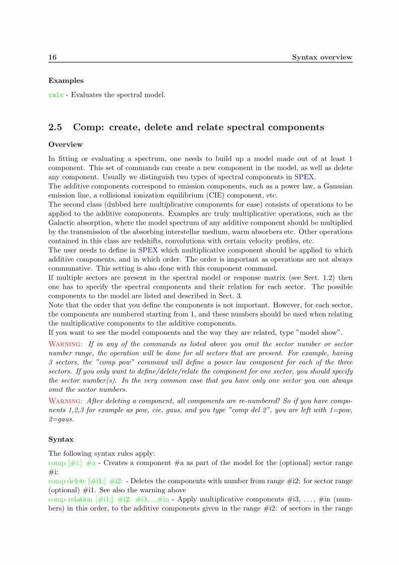
In fitting or evaluating a spectrum, one needs to build up a model made out of at least 1component. This set of commands can create a new component in the model, as well as deleteany component. Usually we distinguish two types of spectral components in SPEX.
The additive components correspond to emission components, such as a power law, a Gaussianemission line, a collisional ionization equilibrium (CIE) component, etc.
The second class (dubbed here multiplicative components for ease) consists of operations to beapplied to the additive components. Examples are truly multiplicative operations, such as theGalactic absorption, where the model spectrum of any additive component should be multipliedby the transmission of the absorbing interstellar medium, warm absorbers etc. Other operationscontained in this class are redshifts, convolutions with certain velocity profiles, etc.
The user needs to define in SPEX which multiplicative component should be applied to whichadditive components, and in which order. The order is important as operations are not alwayscommunative. This setting is also done with this component command.
If multiple sectors are present in the spectral model or response matrix (see Sect. 1.2) thenone has to specify the spectral components and their relation for each sector. The possiblecomponents to the model are listed and described in Sect. 3.
Note that the order that you define the components is not important. However, for each sector,the components are numbered starting from 1, and these numbers should be used when relatingthe multiplicative components to the additive components.
If you want to see the model components and the way they are related, type ”model show”.
Warning: If in any of the commands as listed above you omit the sector number or sectornumber range, the operation will be done for all sectors that are present. For example, having3 sectors, the ”comp pow” command will define a power law component for each of the threesectors. If you only want to define/delete/relate the component for one sector, you should specifythe sector number(s). In the very common case that you have only one sector you can alwaysomit the sector numbers.
Warning: After deleting a component, all components are re-numbered! So if you have compo-nents 1,2,3 for example as pow, cie, gaus, and you type ”comp del 2”, you are left with 1=pow,2=gaus.
Syntax
The following syntax rules apply:
comp [#i:] #a - Creates a component #a as part of the model for the (optional) sector range#i:comp delete [#i1:] #i2: - Deletes the components with number from range #i2: for sector range(optional) #i1. See also the warning abovecomp relation [#i1:] #i2: #i3,...,#in - Apply multiplicative components #i3, . . . , #in (num-bers) in this order, to the additive components given in the range #i2: of sectors in the range

2.6 Data: read response file and spectrum 17
#i1 (optional). Note that the multiplicative components must be separated by a ”,”
Examples
comp pow - Creates a power-law component for modeling the spectrum for all sectors that arepresent.comp 2 pow - Same as above, but now the component is created for sector 2.comp 4:6 pow - Create the power law for sectors 4, 5 and 6com abs - Creates a Morrison & McCammon absorption component.comp delete 2 - Deletes the second created component. For example, if you have 1 = pow, 2= cie and 3 = gaus, this command delets the cie component and renumbers 1 = pow, 2 = gauscomp del 1:2 - In the example above, this will delete the pow and cie components and renum-bers now 1 = gauscomp del 4:6 2 - If the above three component model (pow, cie, gaus) would be defined for 8sectors (numbered 1–8), then this command deletes the cie component (nr. 2) for sectors 4–6only.comp rel 1 2 - Apply component 2 to component 1. For example, if you have defined beforewith ”comp pow” and ”comp ”abs” a power law and galactic absorption, the this command tellsyou to apply component 2 (abs) to component 1 (pow).comp rel 1 5,3,4 - Taking component 1 a power law (pow), component 3 a redshift operation(reds), component 4 galactic absorption (abs) and component 5 a warm absorber (warm), thiscommand has the effect that the power law spectrum is multiplied first by the transmission ofthe warm absorber (5=warm), then redshifted (3=reds) and finally multiplied by the transmis-sion of our galaxy (4=abs). Note that the order is always from the source to the observer!comp rel 1:2 5,3,4 - Taking component 1 a power law (pow), component 2 a gaussian line(gaus), and 3–5 as above, this model applies multiplicative components 5, 3 and 4 (in that orer)to the emission spectra of both component 1 (pow) and 2 (cie).comp rel 7:8 1:2 5,3,4 - As above, but only for sectors 7 and 8 (if those are defined)
2.6 Data: read response file and spectrum
Overview
In order to fit an observed spectrum, SPEX needs a spectral data file and a response matrix.These data are stored in FITS format, tailored for SPEX (see section 7.7). The data files neednot necessarily be located in the same directory, one can also give a pathname plus filename inthis command.
Syntax
The following syntax rules apply: data #a1 #a2 - Read response matrix #a1 and spectrum#a2data delete instrument #i - Remove instrument #i from the data setdata merge sum #i: - Merge instruments in range #i: to a single spectrum and response matrix,by adding the data and matricesdata merge aver #i: - Merge instruments in range #i: to a single spectrum and response matrix,

18 Syntax overview
by averaging the data and matricesdata save #i #a [overwrite] - Save data #a from instrument #i with the option to overwrite theexistent file. SPEX automatically tags the .spo extension to the given file name. No responsefile is saved.data show - Shows the data input given, as well as the count (rates) for source and background,the energy range for which there is data the response groups and data channels. Also the inte-gration time and the standard plotting options are given.
Examples
data mosresp mosspec - read a spectral response file named mosresp.res and the correspondingspectral file mosspec.spo. Hint, although 2 different names are used here for ease of understand-ing, it is eased if the spectrum and response file have the same name, with the appropriateextension.data delete instrument 1 - delete the first instrumentdata merge aver 3:5 - merge instruments 3–5 into a single new instrument 3 (replacing theold instrument 3), by averaging the spectra. Spectra 3–5 could be spectra taken with the sameinstrument at different epochs.data merge sum 1:2 - add spectra of instruments 1–2 into a single new instrument 1 (replacingthe old instrument 1), by adding the spectra. Useful for example in combining XMM-NewtonMOS1 and MOS2 spectra.data save 1 mydata - Saves the data from instrument 1 in the working directory under thefilename of mydata.spodata /mydir/data/mosresp /mydir/data/mosspec - read the spectrum and response from thedirectory /mydir/data/
2.7 DEM: differential emission measure analysis
Overview
SPEX offers the opportunity to do a differential emission measure analysis. This is an effectiveway to model multi-temperature plasmas in the case of continuous temperature distributions ora large number of discrete temperature components.
The spectral model can only have one additive component: the DEM component that corre-sponds to a multi-temperature structure. There are no restrictions to the number of multiplica-tive components. For a description of the DEM analysis method see document SRON/SPEX/TRPB05(in the documentation for version 1.0 of SPEX) Mewe et al. (1994) and Kaastra et al. (1996).
SPEX has 5 different dem analysis methods implemented, as listed shortly below. We refer tothe above papers for more details.
1. reg – Regularization method (minimizes second order derivative of the DEM; advantage:produces error bars; disadvantage: needs fine-tuning with a regularization parameter andcan produce negative emission measures.
2. clean – Clean method: uses the clean method that is widely used in radio astronomy.Useful for ”spiky emission measure distributions.

2.7 DEM: differential emission measure analysis 19
3. poly – Polynomial method: approximates the DEM by a polynomial in the log T −− log Yplane, where Y is the emission measure. Works well if the DEM is smooth.
4. mult – Multi-temperature method: tries to fit the DEM to the sum of Gaussian componentsas a function of log T . Good for discrete and slightly broadened components, but may notalways converge.
5. gene – Genetic algorithm: using a genetic algorithm try to find the best solution. Advan-tage: rather robust for avoiding local subminima.Disadvantage: may require a lot of cputime, and each run produces slightly different results (due to randomization).
In practice to use the DEM methods the user should do the following steps:
1. Read and prepare the spectral data that should be analysed
2. Define the dem model with the ”comp dem” command
3. Define any multiplicative models (absorption, redshifts, etc.) that should be applied tothe additive model
4. Define the parameters of the dem model: number of temperature bins, temperature range,abundances etc.
5. give the ”dem lib” command to create a library of isothermal spectra.
6. do the dem method of choice (each one of the five methods outlined above)
7. For different abundances or parameters of any of the spectral components, first the ”demlib” command must be re-issued!
Syntax
The following syntax rules apply:dem lib - Create the basic DEM library of isothermal spectradem reg auto - Do DEM analysis using the regularization method, using an automatic searchof the optimum regularization parameter. It determines the regularisation parameter R in sucha way that χ2(R) = χ2(0)[1 + s
√
2/(n − nT] where the scaling factor s = 1, n is the numberof spectral bins in the data set and nT is the number of temperature components in the DEMlibrary.dem reg auto #r - As above, but for the scaling factor s set to #r.dem reg #r - Do DEM analysis using the regularization method, using a fixed regularizationparameter R =#r.dem chireg #r1 #r2 #i - Do a grid search over the regularization parameter R, with #i stepsand R distributed logarithmically between #r1 and #r2. Useful to scan the χ2(R) curve when-ever it is complicated and to see how much ”penalty’ (negative DEM values) there are for eachvalue of R.dem clean - Do DEM analysis using the clean methoddem poly #i - Do DEM analysis using the polynomial method, where #i is the degree of thepolynomialdem mult #i - Do DEM analysis using the multi-temperature method, where #i is the numberof broad components

20 Syntax overview
dem gene #i1 #i2 - Do DEM analysis using the genetic algorithm, using a population size givenby #i1 (maximum value 1024) and #i2 is the number of generations (no limit, in practice after∼100 generations not much change in the solution. Experiment with these numbers for yourpractical case.dem read #a - Read a DEM distribution from a file named #a which automatically gets theextension ”.dem”. It is an ascii file with at least two columns, the first column is the temperaturein keV and the second column the differential emission measure, in units of 1064 m−3 keV−1.The maximum number of data points in this file is 8192. Temperature should be in increasingorder. The data will be interpolated to match the temperature grid defined in the dem model(which is set by the user).dem save #a - Save the DEM to a file #a with extension ”.dem”. The same format as above isused for the file. A third column has the corresponding error bars on the DEM as determinedby the DEM method used (not always relevant or well defined, exept for the regularizationmethod).dem smooth #r - Smoothes a DEM previously determined by any DEM method using a blockfilter/ Here #r is the full width of the filter expressed in 10 log T . Note that this smoothing willin principle worsen the χ2 of the solution, but it is sometimes useful to ”wash out” some residualnoise in the DEM distribution, preserving total emission measure.
Examples
dem lib - create the DEM librarydem reg auto - use the automatic regularization methoddem reg 10. - use a regularization parameter of R = 10 in the regularization methoddem chireg 1.e-5 1.e5 11 - do a grid search using 11 regularisation parameters R given by10−5, 10−4, 0.001, 0.01, 0.1, 1, 10, 100, 1000, 104, 105.dem clean - use the clean methoddem poly 7 - use a 7th degree polynomial methoddem gene 512 128 - use the genetic algorithm with a population of 512 and 128 generationsdem save mydem - save the current dem on a file named mydem.demdem read modeldem - read the dem from a file named modeldem.demdem smooth 0.3 - smooth the DEM to a temperature width of 0.3 in 10 log T (approximately afactor of 2 in temperature range).
2.8 Distance: set the source distance
Overview
One of the main principles of SPEX is that spectral models are in principle calculated at thelocation of the X-ray source. Once the spectrum has been evaluated, the flux received at Earthcan be calculated. In order to do that, the distance of the source must be set.
SPEX allows for the simultaneous analysis of multiple sky sectors. In each sector, a differentspectral model might be set up, including a different distance. For example, a foreground objectthat coincides partially with the primary X-ray source has a different distance value.
The user can specify the distance in a number of different units. Allowed distance units areshown in the table below.

2.8 Distance: set the source distance 21
Table 2.3: SPEX distance units
Abbrevation Unit
spex internal SPEX units of 1022 m (this is the default)m meterau Astronomical Unit, 1.49597892 1011 mly lightyear, 9.46073047 1015 mpc parsec, 3.085678 1016 mkpc kpc, kiloparsec, 3.085678 1019 mmpc Mpc, Megaparsec, 3.085678 1022 mz redshift units for the given cosmological parameterscz recession velocity in km/s for the given cosmological parameters
The default unit of 1022 m is internally used in all calculations in SPEX. The reason is that withthis scaling all calculations ranging from solar flares to clusters of galaxies can be done withsingle precision arithmetic, without causing underflow or overflow. For the last two units (z andcz), it is necessary to specify a cosmological model. Currently this model is simply described byH0, Ωm (matter density), ΩΛ (cosmological constant related density), and Ωr (radiation density).At startup, the values are:
H0: 70 km/s/Mpc ,
Ωm: 0.3 ,
ΩΛ: 0.7 ,
Ωr: 0.0
i.e. a flat model with cosmological constant. However, the user can specify other values of thecosmological parameters. Note that the distance is in this case the luminosity distance.
Note that the previous defaults for SPEX (H0 = 50, q0 = 0.5) can be obtained by puttingH0 = 50, Ωm = 1, ΩΛ = 0 and Ωr = 0.
Warning: when H0 or any of the Ω is changed, the luminosity distance will not change, but theequivalent redshift of the source is adjusted. For example, setting the distance first to z=1 withthe default H0=70 km/s/Mpc results into a distance of 2.039 1026 m. When H0 is then changedto 100 km/s/Mpc, the distance is still 2.168 1026 m, but the redshift is adjusted to 1.3342.
Warning: In the output also the light travel time is given. This should not be confused withthe (luminosity) distance in light years, which is simply calculated from the luminosity distancein m!
Syntax
The following syntax rules apply to setting the distance:
distance [sector #i:] #r [#a] - set the distance to the value #r in the unit #a. This optionaldistance unit may be omittted. In that case it is assumed that the distance unit is the defaultSPEX unit of 1022 m. The distance is set for the sky sector range #i:. When the optional sectorrange is omitted, the distance is set for all sectors.distance show - displays the distance in various units for all sectors.distance h0 #r - sets the Hubble constant H0 to the value #r.

22 Syntax overview
distance om #r - sets the Ωm parameter to the value #r.distance ol #r - sets the ΩΛ parameter to the value #r.distance or #r - sets the Ωr parameter to the value #r.
Examples
distance 2 - sets the distance to 2 default units, i.e. to 2E22 m.distance 12.0 pc - sets the distance for all sectors to 12 pc.distance sector 3 0.03 z - sets the distance for sector 3 to a redshift of 0.03.distance sector 2 : 4 50 ly - sets the distance for sectors 2-4 to 50 lightyear.distance h0 50. - sets the Hubble constant to 50 km/s/Mpc.distance om 0.27 - sets the matter density parameter Ωm to 0.27distance show - displays the distances for all sectors, see the example below for the outputformat.
SPEX> di 100 mpc
Distances assuming H0 = 70.0 km/s/Mpc, Omega_m = 0.300 Omega_Lambda = 0.700 Omega_r = 0.000
Sector m A.U. ly pc kpc Mpc redshift cz age(yr)
----------------------------------------------------------------------------------------------
1 3.086E+24 2.063E+13 3.262E+08 1.000E+08 1.000E+05 100.0000 0.0229 6878.7 3.152E+08
----------------------------------------------------------------------------------------------
2.9 Egrid: define model energy grids
Overview
SPEX operates essentially in two modes: with an observational data set (read using the data commands),or without data, i.e. theoretical model spectra. In the first case, the energy grid neede to evaluate thespectra is taken directly from the data set. In the second case, the user can choose his own energy grid.The energy grid can be a linear grid, a logarithmic grid or an arbitrary grid read from an ascii-file. Itis also possible to save the current energy grid, whatever that may be. In case of a linear or logarithmicgrid, the lower and upper limit, as well as the number of bins or the step size must be given.The following units can be used for the energy or wavelength: keV (the default), eV, Ryd, J, Hz, A, nm.When the energy grid is read or written from an ascii-file, the file must have the extension ”.egr”, andcontains the bin boundaries in keV, starting from the lower limit of the first bin and ending with theupper limit for the last bin. Thus, the file has 1 entry more than the number of bins! In general, theenergy grid must be increasing in energy and it is not allowed that two neighbouring boundaries havethe same value.Finally, the default energy grid at startup of SPEX is a logarithmic grid between 0.001 and 100 keV,with 8192 energy bins.
Syntax
The following syntax rules apply:egrid lin #r1 #r2 #i [#a] - Create a linear energy grid between #r1 and #r2, in units given by #a (aslisted above). If no unit is given, it is assumed that the limits are in keV. The number of energy bins isgiven by #iegrid lin #r1 #r2 step #r3 [#a] - as above, but do not prescribe the number of bins, but the bin width#r3. In case the difference between upper and lower energy is not a multiple of the bin width, the upperboundary of the last bin will be taken as close as possible to the upper boundary (but cannot be equal

2.10 Elim: set flux energy limits 23
to it).egrid log #r1 #r2 #i [#a] - Create a logarithmic energy grid between #r1 and #r2, in units given by#a (as listed above). If no unit is given, it is assumed that the limits are in keV. The number of energybins is given by #iegrid log #r1 #r2 step #r3 [#a] - as above, but do not prescribe the number of bins, but the bin width(in log E) #r3.egrid read #a - Read the energy grid from file #a.egregrid save #a - Save the current energy grid to file #a.egr
Warning: The lower limit of the energy grid must be positive, and the upper limit must always be largerthan the lower limit.
Examples
egrid lin 5 38 step 0.02 a - create a linear energy grid between 5− 38 A, with a step size of 0.02 A.egrid log 2 10 1000 - create a logarithmic energy grid with 1000 bins between 2 − 10 keV.egrid log 2 10 1000 ev - create a logarithmic energy grid with 1000 bins between 0.002− 0.010 keV.egrid read mygrid - read the energy grid from the file mygrid.egr.egrid save mygrid - save the current energy grid to file mygrid.egr.
2.10 Elim: set flux energy limits
Overview
SPEX offers the opportunity to calculate the model flux in a given energy interval for the current spectralmodel. This information can be viewed when the model parameters are shown (see section 2.21).
For each additive component of the model, the following quantities are listed:
the observed photon number flux (photonsm−2 s−1) at earth, including any effects of galactic absorptionetc.
the observed energy flux (Wm−2) at earth, including any effects of galactic absorption etc.
the intrinsic number of photons emitted at the source, not diluted by any absorption etc., in photons s−1.
the intrinsic luminosity emitted at the source, not diluted by any absorption etc., in W.
The following units can be used to designate the energy or wavelength range: keV (the default), eV, Ryd,J, Hz, A, nm.
Syntax
The following syntax rules apply:
elim #r1 #r2 [#a] - Determine the flux between #r1 #r2, in units given by #a, and as listed above.The default at startup is 2 − 10 keV. If no unit is given, it is assumed that the limits are in keV.
Warning: When new units or limits are chosen, the spectrum must be re-evaluated (e.g. by giving the”calc” comand) in order to determine the new fluxes.
Warning: The lower limit must be positive, and the upper limit must always be larger than the lowerlimit.
24 Syntax overview
Examples
elim 0.5 4.5 - give fluxes between 0.5 and 4.5 keVelim 500 4500 ev - give fluxes between 500 and 4500 eV (same result as above)elim 5 38 a - give fluxes in the 5 to 38 A wavelength band
2.11 Error: Calculate the errors of the fitted parameters
Overview
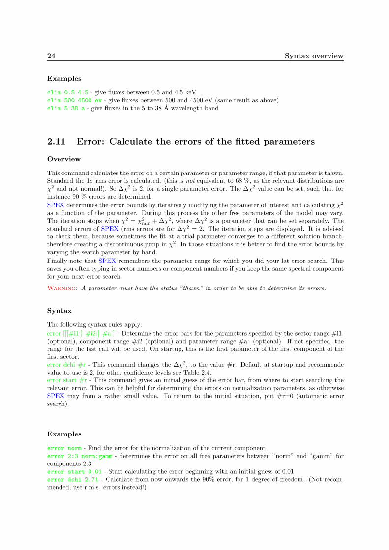
This command calculates the error on a certain parameter or parameter range, if that parameter is thawn.Standard the 1σ rms error is calculated. (this is not equivalent to 68 %, as the relevant distributions areχ2 and not normal!). So ∆χ2 is 2, for a single parameter error. The ∆χ2 value can be set, such that forinstance 90 % errors are determined.
SPEX determines the error bounds by iteratively modifying the parameter of interest and calculating χ2
as a function of the parameter. During this process the other free parameters of the model may vary.The iteration stops when χ2 = χ2
min + ∆χ2, where ∆χ2 is a parameter that can be set separately. Thestandard errors of SPEX (rms errors are for ∆χ2 = 2. The iteration steps are displayed. It is advisedto check them, because sometimes the fit at a trial parameter converges to a different solution branch,therefore creating a discontinuous jump in χ2. In those situations it is better to find the error bounds byvarying the search parameter by hand.
Finally note that SPEX remembers the parameter range for which you did your lat error search. Thissaves you often typing in sector numbers or component numbers if you keep the same spectral componentfor your next error search.
Warning: A parameter must have the status ”thawn” in order to be able to determine its errors.
Syntax
The following syntax rules apply:
error [[[#i1:] #i2:] #a:] - Determine the error bars for the parameters specified by the sector range #i1:(optional), component range #i2 (optional) and parameter range #a: (optional). If not specified, therange for the last call will be used. On startup, this is the first parameter of the first component of thefirst sector.error dchi #r - This command changes the ∆χ2, to the value #r. Default at startup and recommendevalue to use is 2, for other confidence levels see Table 2.4.error start #r - This command gives an initial guess of the error bar, from where to start searching therelevant error. This can be helpful for determining the errors on normalization parameters, as otherwiseSPEX may from a rather small value. To return to the initial situation, put #r=0 (automatic errorsearch).
Examples
error norm - Find the error for the normalization of the current componenterror 2:3 norm:gamm - determines the error on all free parameters between ”norm” and ”gamm” forcomponents 2:3error start 0.01 - Start calculating the error beginning with an initial guess of 0.01error dchi 2.71 - Calculate from now onwards the 90% error, for 1 degree of freedom. (Not recom-mended, use r.m.s. errors instead!)

2.12 Fit: spectral fitting 25
Table 2.4: ∆χ2 as a function of confidence level, P, and degrees of freedom, ν.
νP 1 2 3 4 5 6
68.3% 1.00 2.30 3.53 4.72 5.89 7.0490% 2.71 4.61 6.25 7.78 9.24 10.695.4% 4.00 6.17 8.02 9.70 11.3 12.899% 6.63 9.21 11.3 13.3 15.1 16.899.99% 15.1 18.4 21.1 13.5 25.7 27.8
2.12 Fit: spectral fitting
Overview
With this command one fits the spectral model to the data. Only parameters that are thawn are changedduring the fitting process. Options allow you to do a weighted fit (according to the model or the data),have the fit parameters and plot printed and updated during the fit, and limit the number of iterationsdone.Here we make a few remarks about proper data weighting. χ2 is usually calculated as the sum over alldata bins i of (Ni − si)
2/σ2i , i.e.
χ2 =
n∑
i=1
(Ni − si)2
σ2i
, (2.1)
where Ni is the observed number of source plus background counts, si the expected number of sourceplus background counts of the fitted model, and for Poissonian statistics usually one takes σ2
i = Ni.Take care that the spectral bins contain sufficient counts (either source or background), recommendedis e.g. to use at least ∼10 counts per bin. If this is not the case, first rebin the data set whenever youhave a ”continuum” spectrum. For line spectra you cannot do this of course without loosing importantinformation! Note however that this method has inaccuracies if Ni is less than ∼100.Wheaton et al. ([1995]) have shown that the classical χ2 method becomes inaccurate for spectra withless than ∼ 100 counts per bin. This is not due to the approximation of the Poisson statistic by a normaldistribution, but due to using the observed number of counts Ni as weights in the calculation of χ2.Wheaton et al. showed that the problem can be resolved by using instead σ2
i = si, i.e. the expectednumber of counts from the best fit model.The option ”fit weight model” allows to use these modified weights. By selecting it, the expected numberof counts (both source plus background) of the current spectral model is used onwards in calculating thefit statistic. Wheaton et al. suggest to do the following 3-step process, which we also recommend to theuser of SPEX:
1. first fit the spectrum using the data errors as weights (the default of SPEX).
2. After completing this fit, select the ”fit weight model” option and do again a fit
3. then repeat this step once more by again selecting ”fit weight model” in order to replace si of thefirst step by si of the second step in the weights. The result should now have been converged (underthe assumption that the fitted model gives a reasonable description of the data, if your spectralmodel is way off you are in trouble anyway!).
There is yet another option to try for spectral fitting with low count rate statistics and that is maximumlikelyhood fitting. It can be shown that a good alternative to χ2 in that limit is
C = 2
n∑
i=1
si −Ni +Ni ln(Ni/si). (2.2)

26 Syntax overview
This is strictly valid in the limit of Poissonian statistics. If you have a background subtracted, take carethat the subtracted number of background counts is properly stored in the spectral data file, so that rawnumber of counts can be reconstructed.
Syntax
The following syntax rules apply:fit - Execute a spectral fit to the data.fit print #i - Printing the intermediate results during the fitting to the screen for every n-th step, withn=#i (most useful for n = 1). Default value: 0 which implies no printing of intermediate steps.fit iter #i - Stop the fitting process after #i iterations, regardless convergence or not. This is useful toget a first impression for very cpu-intensive models. To return to the default stop criterion, type fit iter0.fit weight model - Use the current spectral model as a basis for the statistical weight in all subsequentspectral fitting.fit weight data - Use the errors in the spectral data file as a basis for the statistical weight in all subse-quent spectral fitting. This is the default at the start of SPEX.fit method classical - Use the classical Levenberg-Marquardt minimisation of χ2 as the fitting method.This is the default at start-up.fit method cstat - Use the C-statistics instead of χ2 for the minimisation.
Examples
fit - Performs a spectral fit. At the end the list of best fit parameters is printed, and if there is a plotthis will be updated.fit print 1 - If followed by the above fit command, the intermediate fit results are printed to the screen,and the plot of spectrum, model or residuals is updated (provided a plot is selected).fit iter 10 - Stop the after 10 iterations or earlier if convergence is reached before ten iterations arecompleted.fit iter 0 - Stop fitting only after full convergence (default).fit weight model - Instead of using the data for the statistical weights in the fit, use the current model.fit weight data - Use the data instead for the statistical weights in the fit.fit method cstat - Switch from χ2 to C-statistics.fit method clas - Switch back to χ2 statistics.
2.13 Ibal: set type of ionisation balance
Overview
For the plasma models, different ionisation balance calculations are possible.Currently, the default set is Arnaud & Rothenflug ([1985]) for H, He, C, N, O, Ne, Na, Mg, Al, Si, S, Ar,Ca and Ni, with Arnaud & Raymond ([1992]) for Fe. Table 2.5 lists the possible options.
Table 2.5: Ionisation balance modes
Abbrevation Reference
reset default (=ar92)ar85 Arnaud & Rothenflug ([1985])ar92 Arnaud & Raymond ([1992]) for Fe,
Arnaud & Rothenflug ([1985]) for the other elements

2.14 Ignore: ignoring part of the spectrum 27
Syntax
The following syntax rules apply:ibal #a - Set the ionisation balance to set #a with #a in the table above.
Examples
ibal reset - Take the standard ionisation balanceibal ar85 - Take the Arnaud & Rothenflug ionisation balance
2.14 Ignore: ignoring part of the spectrum
Overview
If one wants to ignore part of a data set in fitting the input model, as well as in plotting this commandshould be used. The spectral range one wants to ignore can be specified as a range in data channels or arange in wavelength or energy. Note that the first number in the range must always be smaller or equalto the second number given. If multiple instruments are used, one must specify the instrument as well.If the data set contains multiple regions, one must specify the region as well. So per instrument/regionone needs to specify which range to ignore. The standard unit chosen for the range of data to ignore isdata channels. To undo ignore, see the use command (see section 2.30).The range to be ignored can be specified either as a channel range (no units required) or in eiter any ofthe following units: keV, eV, Rydberg, Joule, Hertz, A, nanometer, with the following abbrevations: kev,ev, ryd, j, hz, ang, nm.
Syntax
The following syntax rules apply:ignore [instrument #i1] [region #i2] #r - Ignore a certain range #r given in data channels of instrument#i1 and region #i2. The instrument and region need to be specified if there are more than 1 data setsin one instrument data set or if there are more than 1 data set from different instruments.ignore [instrument #i1] [region #i2] #r unit #a - Same as the above, but now one also specifies the unites#a in which the range #r of data points to be ignored are given. The units can be either A(ang) or (k)eV.
Examples
ignore 1000:1500 - Ignores data channels 1000 till 1500.ignore region 1 1000:1500 - Ignore data channels 1000 till 1500 for region 1.ignore instrument 1 region 1 1000:1500 - Ignores the data channels 1000 till 1500 of region 1 fromthe first instrument.ignore instrument 1 region 1 1:8 unit ang - Same as the above example, but now the range isspecified in units of A instead of in data channels.ignore 1:8 unit ang - Ignores the data from 1 to 8 A, only works if there is only one instrument andone region included in the data sets.
2.15 Ion: select ions for the plasma models
Overview
For the plasma models, it is possible to include or exclude specific groups of ions from the line calulations.This is helpful if a better physical understanding of the (atomic) physics behind the spectrum is requested.

28 Syntax overview
Currently these settings only affect the line emission; in the calculation of the ionisation balance as wellas the continuum always all ions are taken into account (unless of course the abundance is put to zero).
Syntax
The following syntax rules apply:
ions show - Display the list of ions currently taken into accountions use all - Use all possible ions in the line spectrumions use iso #i: - Use ions of the isoelectronic sequences indicated by #i: in the line spectrumions use z #i: - Use ions with the atomic numbers indicated by #i: in the line spectrumions use ion #i1 #i2: - Use ions with the atomic number indicated by #i1 and ionisation stage indicatedby #i2: in the line spectrumions ignore all - Ignore all possible ions in the line spectrumions ignore iso #i: - Ignore ions of the isoelectronic sequences indicated by #i: in the line spectrumions ignore z #i: - Ignore ions with the atomic numbers indicated by #i: in the line spectrumions ignore ion #i1 #i2: - Ignore ions with the atomic number indicated by #i1 and ionisation stageindicated by #i2: in the line spectrum
Examples
ions ignore all - Do not take any line calculation into accountions use iso 3 - Use ions from the Z = 3 (Li) isoelectronic sequenceions use iso 1:2 - Use ions from the H-like and He-like isoelectronic sequencesions ignore z 26 - Ignore all iron (Z = 26) ionsions use ion 6 5:6 - Use C V to C VIions show - Display the list of ions that are used
2.16 Log: Making and using command files
Overview
In many circumstances a user of SPEX wants to repeat his analysis for a different set of parameters. Forexample, after having analysed the spectrum of source A, a similar spectral model and analysis could betried on source B. In order to facilitate such analysis, SPEX offers the opportunity to save the commandsthat were used in a session to an ascii-file. This ascii-file in turn can then be read by SPEX to executethe same list of commands again, or the file may be edited by hand.
The command files can be nested. Thus, at any line of the command file the user can invoke the executionof another command file, which is executed completely before execution with the current command fileis resumed. Using nested command files may help to keep complex analyses manageable, and allow theuser easy modification of the commands.
For example, the user may have a command file named run which does his entire analysis. This commandfile might start with the line ”log exe mydata” that will run the command file mydata that contains allinformation regarding to the data sets read, further data selection or binning etc. This could be followedby a second line in run like ”log exe mymodel” that runs the command file mymodel which could containthe set-up for the spectral model and/or parameters. Also, often used plot settings (e.g. stacking ofdifferent plot types) could easily placed in separate command files.
In order to facilitate the readability of the command files, the user can put comment lines in the commandfiles. Comment lines are recognized by the first character, that must be #. Also blank lines are allowedin the command file, in order to enhance (human) readability.
In general, all commands entered by the user are stored on the command file. Exceptions are thecommands read from a nested command file (it is not necessary to save these commands, since they are

2.17 Menu: Menu settings 29
already in the nested command file). Also, help calls and the command to open the file (”log save #a”)are not stored.
Before saving, all commands are expanded to the full keywords, in those cases where abbrevated com-mands were used. However, for execution this is not important, since the interpreter can read bothabbrevated and full keywords.
When a command file is read and the end of file is reached, the text ”Normal end of command fileencountered” is printed on the screen, and execution of the calling command file is resumed, or if thecommand file was opened from the terminal, control is passed over to the terminal again.
Finally, it is also possible to store all the output that is printed on the screen to a file. This is usefull forlong sessions or for computer systems with a limited screen buffer. The output saved this way could beinspected later by (other programs of) the user. It is also usefull if SPEX is run in a kind of batch-mode.
Syntax
The following syntax rules apply for command files:
log exe #a - Execute the commands from the file #a. The suffix ”.com” will be automatically appendedto this filename.log save #a [overwrite] [append] - Store all subsequent commands on the file #a. The suffix ”.com” willbe automatically appended to this filename. The optional argument ”overwrite” will allow to overwritean already existing file with the same name. The argument ”append” indicates that if the file alreadyexists, the new commands will be appended at the end of this file.log close save - Close the current command file where commands are stored. No further commands willbe written to this file.log out #a [overwrite] [append] - Store all subsequent screen output on the file #a. The suffix ”.out” willbe automatically appended to this filename. The optional argument ”overwrite” will allow to overwritean already existing file with the same name. The argument ”append” indicates that if the file alreadyexists, the new output will be appended at the end of this file.log close output - Close the current ascii file where screen output is stored. No further output will bewritten to this file.
Examples
log save myrun - writes all subsequent commands to a new file named ”myrun.com”. However, in casethe file already exists, nothing is written but the user gets a warning instead.log save myrun append - as above, but appends it to an existing filelog save myrun overwrite - as above, but now overwrites without warning any already existing filewith the same name.log close save - close the file where commands are stored.log exe myrun - executes the commands in file myrun.com.log output myrun - writes all subsequent output to file myrun.out.log close output - closes the file above.
2.17 Menu: Menu settings
Overview
When command lines are typed, it frequently happens that often the first keywords are identical forseveral subsequent lines. This may happen for example when a plot is edited. SPEX offers a shortcut tothis by using the menu command.

30 Syntax overview
Syntax
The following syntax rules apply:
menu none - Quit the current menu text settings (i.e., return to the default spex prompt.menu text #a - For all following commands, the text string #a will be appended automatically beforethe following commands
Examples
menu text plot - All following commants will get the ”plot” keyword put in front of them. So if thenext commant would be ”plot dev xs” it is sufficient to type ”dev xs” instead.menu none - Return to the normal SPEX prompt.menu text "par 1 2" - All following commands wil get the ”par 1 2” keywords put in front of them.The next command could be ”t val 4.”, which will be expanded to the full ”par 1 2 t val 4.” to set thetemperature of sector 1, component 2 to 4 keV. Note that here the text has three keywords (par, 1, 2)and hence it has to be put between ””, to indicate that it is a single text string. If there is only onekeyword, these ”” are not necessary.
2.18 Model: show the current spectral model
Overview
This commands prints the current spectral model, for each sector, to the screen. The model is the set ofspectral components that is used, including all additive and multiplicative components. For all additivecomponents, it shows in which order the multiplicative components are applied to the additive (emitted)components. See Sect. 2.5 for more details.
Syntax
The following syntax rules apply:
model show - Prints the model for all sectors to the screen.model show #i - Prints the model for sector #i to the screen.
Examples
model show 2 - Prints the model for the second sector
2.19 Multiply: scaling of the response matrix
Overview
This command multiplies (a component of) the response matrix by a constant.
Warning: If this command is repeated for the same component then the original response matrix ischanged by the multiplication of the constants. For example, after multiplying the response matrix by afactor of 2, the original matrix is recovered by multiplying the intermediate result by 0.5.
Warning: The instrument number must be given in this command even if you use only a single instru-ment.

2.20 Obin: optimal rebinning of the data 31
Syntax
The following syntax rules apply:multiply #i1 [component #i2] #r - Multiplies the response matrix of component #i2 of instrument #i1by a constant #r.
Examples
multiply 1 3.5 - Multiplies the response matrix from instrument 1 by a factor of 3.5.multiply 1 component 2 3.5 - Multiplies the second component of instrument 1 by the constant 3.5.
2.20 Obin: optimal rebinning of the data
Overview
This command rebins (a part of) the data (thus both the spectrum and the response) to the optimalbin size given the statistics of the source as well as the instrumental resolution. This is recommendedto do in all cases, in order to avoid oversampling of the data. The theory and algorithms used for thisrebinning ared escribed in detail in Sect. ??. A simple cartoon of this is: binning to 1/3 of the FWHM,but the factor of 1/3 depends weakly upon the local count rate at the given energy and the number ofresolution elements. The better the statistics, the smaller the bin size.
Syntax
The following syntax rules apply:obin #i1: - Simplest command allowed. #i1: is the range in data channels over which the binning needsto take place.obin #r1: #i: unit #a - The same command as above, except that now the ranges over which the datais to be binned (#r1:) are specified in units (#a) different from data channels. These units can be eV,keV, A, as well as in units of Rydberg (ryd), Joules (j), Hertz (hz) and nanometers (nm).obin [instrument #i1:] [region #i2:] #i3: - Here #i3: is the same as #i1: in the first command.However, here one can specify the instrument range #i1: and the region range #i2: as well, so that thebinning is done only for one given data set.obin [instrument #i1:] [region #i2:] #r1: [unit #a] - This command is the same as the above, except thathere one can specify the range over which the binning should occur in the units specified by #a. Theseunits can be eV, A, keV, as well as in units of Rydberg (ryd), Joules (j), Hertz (hz) and nanometers (nm).
Examples
obin 1:10000 - Optimally bins the data channels 1:10000.obin 1:4000 unit ev - Does the same as the above, but now the data range to be binned is given ineV, from 1−4000 eV, instead of in data channels.obin instrument 1 region 1 1:19 unit a - Bins the data from instrument 1 and region 1 between 1and 19 A.
2.21 Par: Input and output of model parameters
Overview
This command is used as an interface to set or display the parameters of the spectral model. Each modelparameter (like temperature T , abundance, normalization etc.) has a set of attributes, namely its value,

32 Syntax overview
status, range and coupling. This is illustrated by the following example. Assume we have a spectralmodel consisting of a thermal plasma. Consider the silicon abundance (acronym in the model: 14). Itcan have a value (for example 2.0, meaning twice the solar abundance). Its status is a logical variable,true (thawn) if the parameter can be adjusted during the spectral fitting proces or false (frozen) if itshould be kept fixed during the spectral fit. The range is the allowed range that the parameter canhave during the spectral fit, for example 0–1000 (minimum – maximum values). This is useful to setto constrain a spectral search to a priori ”reasonable” values (e.g. abundances should be non-negative)or ”safe” values (SPEX could crash for negative temperatures for example). Finally the coupling allowsyou to couple parameters, for example if the Si abundance is coupled to the Fe abundance, a change inthe Fe abundance (either defined by the user or in a spectral fitting process) will result automaticallyin an adjustment of the Si abundance. This is a useful property in practical cases where for example aspectrum has strong Fe lines and weaker lines from other species, but definitely non-solar abundances.In this case, one may fit the Fe abundance, but the statistics for the other elements may not be sufficientto determine their abundance accurately; however a priori insight might lead you to think that it is theglobal metallicity that is enhanced, and therefore you would expect the Si abundance to be enhanced inthe same way as Fe.With the par command, you can set for each parameter individually or for a range of parameters in thesame command, their attributes (value, status, range and coupling). Also, you can display the parameterson the screen or write them on a SPEX command file, which allows you to start another run with thecurrent set of parameters.When setting parameters, you can also specify the sector (range) and component (range). For your firstcall, it is assumed that you refer to sector 1, component 1, first parameter. In all subsequent calls ofthe parameter command, it is assumed that you refer to the same sector(s) and component(s) as yourlast call, unless specified differently. This is illustrated by the following example. Suppose you have thefollowing model: power law (component 1), blackbody (component 2) and RGS line broadening (lpro,component 3). If you type in the commands in that order, this is what happens:
• par val 2 – sets the norm (= first parameter) of the power law to value 2
• par gam val 3 – sets the photon index of the power law to value 3
• par 2 t val 2.5 – sets the temperature of the blackbody to 2.5 keV
• par norm val 10 – sets the norm of the blackbody to 10
• par 1:2 norm v 5 – sets the norm of both the PL and BB to 5
• par val 4.2 – sets the norm of both the PL and BB to 4.2
• par 3 file myprofile.dat – sets for the LPRO component the file name with the broadening kernalto myprofile.dat
Syntax
The following syntax rules apply:par [#i1:] [#i2:] [#a1:] avalue #a2 - Assign the value #a2 to the parameters specified by the (rangeof) name(s) #a1 of component range #i2: of sectors #i1:. The sector (range), component (range) andparameter name (range) are optional. If #a2 should be an empty text string, specify the value ”none”(without quotes, and all four characters in lowercase). If thei are not specified, the sector(s), compo-nent(s) and parameter(s) of the last call are used. This command holds for input of text strings. For realnumbers, use the following command (with ”avalue” replaced by ”value” and #a2par [#i1:] [#i2:] [#a:] value #r - Assign the value #r to the parameters specified by the (range of)name(s) #a of component range #i2: of sectors #i1:. The sector (range), component (range) and pa-rameter name (range) are optional. If not specified, the sector(s), component(s) and parameter(s) of thelast call are used.par [#i1:] [#i2:] [#a:] status #l - As above but for the status of a (range of) parameters; #l = T (true,thawn) means a parameter that can be adjusted during a spectral fit, #l = F (false, froze, fixed) meansa parameter that will remain fixed during the spectral fitting.

2.21 Par: Input and output of model parameters 33
par [#i1:] [#i2:] [#a:] range #r1 #r2 - As above but fore the allowed range of the parameter. #r1denotes the lower limit and #r2 denotes the upper limit. Both should be specified.par [#i1:] [#i2:] [#a1:] couple [#i3:] [#i4:] #a2: - Here #i1:, #i2:, #a1: are the sector(s), component(s)and parameter(s) that are to be coupled. The parameter (s) to which they are coupled are specified by#a2: and the optional #i3:, #i4:. If ranges are used, take care that the number of sectors, componentsand parameters on the right and left match.par [#i1:] [#i2:] [#a1:] couple [#i3:] [#i4:] #a2: factor #r - As above, but couple using a scaling factor#r.par [#i1:] [#i2:] #a: decouple - Decouples the parameter(s) #a: of (optional) components #i2: of of(optional) sector(s) #i1:. Inverse operation of the couple command.par show [free] - Shows on the display screen all parameters of all components. If the optional keywordfree is given, shows only parameters with fit status ”T” (true, thawn), i.e., the free parameters in aspectral fit.par write #a [overwrite] - Writes all parameters to a SPEX command file #a. #a should be specifiedwithout extension, SPEX automatically adds the .com extension. If the optional overwrite command isgiven, then the file #a will be overwritten with the new values.
Examples
par val 10 - Sets the value of the current parameter to 10.par t val 4 - Sets the parameter named ”t” to 4.par 06:28 value 0.3 - Sets the parameters named 06:28 (for example the abundances of C (Z = 6), N(Z = 7), . . . Ni (Z = 28)) to the value 0.3.par 2 nh val 0.01 - Sets the parameter named ”nh” of component 2 to the value 0.01par 1 1 norm value 1E8 - Sets parameter named ”norm” of component 1 of sector 1 to the value 108.par file avalue myfile.with.data - sets the ascii-type parameter named ”file” to the value ”my-file.with.data” (without quotes).par file avalue none - sets the ascii-type parameter named ”file” to the value ”” (i.e. an empty string)par status frozen - Sets the fit status of the current parameter to ”frozen” (fixed).par 1 3 t stat thawn - Specifies that parameter ”t” of the third component of the model for sector 1should be left free (thawn) during spectral fitting.par 2 3 gamm range 1.6 1.9 - Limit parameter ”gamm” of component 3 of sector 2 to the range 1.6 –1.9.par norm range -1E8 1E8 - Set the range for the parameter ”norm” between −108 and +108. Thiscommand is necessary if for example the model is a delta line used to mimick an absorption line, whichnormally has a default minimum value of 0. (for an emission line).par 1 1 norm couple 2 1 norm - Couples the norm of the first component for the first sector to thenorm of the first component of the model for the second sector.par 1 1 norm couple 2 1 norm factor 3 - The same command as the above, but now the norm ofthe first component in the model for sector 1 is 3 times the norm of the first component of the model forsector 2. For example, if the norm of the 1st component of sector 2 gets the value 40, then the norm ofthe 1st component of sector 1 will automatically be updated to a value of 3 × 40 = 120.par 3:5 02:30 couple 1 02:30 - Couples the abundances of He–Zn of components 3, 4 and 5 to theHe–Zn abundances of component 1.par norm decouple - Decouples the norm of the current component from whatever it was coupled to.par show - Shows all the parameters of the current model for all sectors and how they are coupled (ifapplicable). For each parameter it shows the value, status, range and coupling information, as well asinfo on its units etc. It also shows the fluxes and restframe luminosities of the additive components,photon flux (phot/m**2/s) and energy flux (W/m**2) are the values observed at Earth (including anytransmission effects like Galactic absorption or intrinsic absoprtion that have been taken into account),and the nr. of photons (photons/s) and luminosity (W) are all as emitted by the source, without anyattenuation.par show free - As above, but only displays the parameters that have the status thawn.

34 Syntax overview
par write mypar overwrite - SPEX writes all parameters for the model to a file named mypar.com.Any previously existing file mypar.com is overwritten.par write mypar - Same command as above, but now a new file is created. If there already exists a filewith the same filename SPEX will give an error message.
2.22 Plot: Plotting data and models
Overview
The plot command cause the plot to be (re)drawn on the graphics device. Multiple graphics devices canbe defined in one SPEX session. For example, a plot can be sent to both a postscript and a xs device.A user can also set the number of plot frames in the currently active device(s), e.g. the data and modelcan be displayed in one frame while the residuals can be displayed in a frame below. The user has tospecify what is to be plotted in in each frame.In each plot frame, there can be different sets that can be specified by the ”set” keyword in the plotcommand. For example, for the plot type data, each set corresponds to the spectrum of an instrumentor region; with this option it is therefore possible to give different instruments different colours or plotsymbols, etc., or just to omit one of the instruments from the plot.The plot command is also used to select the axis plot units and scales as well as character commands likefont style, line weights, plot colours, etc. Finally, the plot command can also be used to dump the datato an ascii file.
Warning: To make a plot, always start with a ”plot device” command to open any plot device you wish.Next select a plot type using ”plot type”. After this you can give any plot commands to modify or displaythe plot.
Syntax
The following syntax rules apply for plot:plot - (Re)draws the plot on the graphics device. Take care to open at least one device first (with a ”plotdev” command)plot frame new - Creates a new additional plot frame, where an other plot type can be displayed (or thesame plot type but with different units). Take care to position the viewport of the new and old framesto the desired locations.plot frame #i - Sets frame number #i to be the currently active frame. After this command has beenissued, all plot commands will only affect the currently active frame.plot frame delete #i - Deletes frame number #i.plot type #a - Specifies what is to be plotted in the selected frame. #a can be any of the plot typesspecified in Sect. 5.2.plot device #a1 [#a2] - Selects a graphics device #a1 and optional file name #a2 (in the case of apostscript or gif device). File extensions (for example .ps) should be specified. For valid devices, seeSect. 5.1.plot close #i - Close graphics device number #i. Note, always close a postscript device before quiting/spex, otherwise the contents may be corrupted.plot hlan - Make a hardcopy in landscape orientation and send it to the standard printer. Use is madeof the unix command ”lp -c filename”.plot hpor - As above, but for portrait orientationplot x lin - Plot the x-axis on a linear scaleplot x log - Plot the x-axis on a log scaleplot y lin - Plot the y-axis on a linear scaleplot y log - Plot the y-axis on a log scaleplot y mix #r1 #r2 - Plot the y-axis on a mixed linear/logarithmic scale; for y-values below #r1 thedata will be plotted linear, and for y-values above #r1 the data will be plotted logarithmically; the linearpart occupies the fraction of the total frame height given by #r2. See also Sect. 5.8.2.

2.22 Plot: Plotting data and models 35
plot z lin - Plot the z-axis on a linear scale. The z-axis is defined for two-dimensional plots like contourplots.plot z log - As above, but using a log scale.plot ux #a - Set the plot units on the x-axis, #a can be A, keV, eV or whatever unit that is allowed.The allowed values depend upon the plot type. See Sect. 5.8.1 for allowed units for each plot type.plot uy #a - Same as above, but for the y-axisplot uz #a - Same as above, but for the z-axisplot rx #r1 #r2 - set the plot range on the x-axis from #r1 to #r2plot ry #r1 #r2 - Same as above, but for the y-axisplot rz #r1 #r2 - Same as above, but for the z-axisplot view default #l - For #l is true, the default viewport is used. For #l is false, the default viewport isoverruled and you can specify your own viewport limits with the ”set view x” and ”set view y” commands.Useful for stacking different plot frames.plot view x #r1 #r2 - Set the x viewport range from #r1 to #r2, where #r1 and #r2 must be in therange 0–1.plot view y #r1 #r2 - Same as above, but for the y-range.plot view x1 #r - Set the lower x viewport limit to #rplot view x2 #r - Set the upper x viewport limit to #rplot view y1 #r - Set the lower y viewport limit to #rplot view y2 #r - Set the upper y viewport limit to #rplot view back #i - Set the viewport background colour to value #i. See Sect. 5.3 for the allowed plotcolours.plot view transp #l - If true, set the viewport background to to transparent, the plot frame will be shownwith the background colour selected by the ”plot view back” command. Default is false.plot box disp #l - Display a box around the viewport, true/falseplot box edge #a #l - If true (default), display the edges of the plot box, #a should be one of thefollowing keywords: top, bottom, left, right. Note that whether you see the edges or not also depends onthe settings defined by the ”plot box disp” command.plot box axis x #l - Plots an x-axis with tickmarks at the line y = 0. You only see this of course if youry-range includes the value 0.plot box axis y #l - As above, but for the y-axisplot box grid x #l - Plot a grid for the x-axisplot box grid y #l - Plot a grid for the y-axisplot box ymix #l - Not implemented yetplot box numlab bottom #l - Show the tick number labels at the bottom of the plot, true/falseplot box numlab top #l - Same as above, but for the topplot box numlab left #l - Same as above, but for the leftplot box numlab right #l - Same as above, but for the rightplot box numlab vert #l - Plot the tick number labels on the y-axis vertically or horizontally, set #l totrue for vertical tnumbers and false for horizontal numbers.plot box numlab xscal #i - Way to denote the numerical numbers along the x-axis. Three values areallowed: 0=automatic, 1=forced decimal labeling, 2=forced exponential labeling. Default is 0.plot box numlab yscal #i - As above, but for the y-axisplot box tick invert x #l - Draw the tick marks on the x-axis on the inside or outside the box, set #l totrue for outside and false for inside (default).plot box tick invert y #l - Same as above, but for the y-axis.plot box tick minor x #l - Draw minor tick marks on the x-axis, true/falseplot box tick minor y #l - Same as above, but for the y-axisplot box tick major x #l - Draw major tick marks on the x-axis, true/falseplot box tick major y #l - Same as above, but for the y-axisplot box tick distance x #r - Set the distance between the major/labelled tick marks on the x-axis to #rplot box tick distance y #r - Same as above, but for the y-axisplot box tick subdiv x #i - Draw #i minor tick marks between each major tick mark on the x-axisplot box tick subdiv y #i - Same as above, but for the y-axis

36 Syntax overview
plot box col #i - Set the box colour to colour number #i. See Sect. 5.3 for the allowed plot colours.plot box lt #i - Set the box line type to #i. See Sect. 5.4 for allowed line types.plot box lw #i - Set the box line weight to number #i. See Sect. 5.4 for more about line weights.plot box fh #r - Set the box font height to number #i.plot box font #i - Set the box font to number #i. See Sect. 5.5 for more details about text fonts.plot cap #a disp #l - If #l is true, display the caption (default). For more about captions see Sect. 5.6.Here and below, #a can be x, y, z, id, lt or ut.plot cap #a col #i - Plot caption #a in colour number #i. See Sect. 5.3 for valid colour indices.plot cap #a back #i - Set the background colour for caption #a to #i.plot cap #a lw #i - Set the font line weight for caption #a to #i.plot cap #a fh #r - Set the font height for caption #a to value #r.plot cap #a font #i - Set the font type for caption #a to #i.plot cap #a1 text #a - Set the text for caption #a1 to #a2. Note that the caption text should be putbetween quotion marks, like ”best fit results” if you want to see the text: best fit results.plot cap #a1 side #a2 - Plot caption #a1 at the side of the frame specified by #a2, which may stand fort (top), b (bottom), lh (left, horizontal), rh (right, horizontal), lv (left, vertical) and rv (right, vertical).plot cap #a off #r - Offset caption #a by #r from the edge of the viewport, where #r is in units of thecharacter height. Enter negative values to write inside the viewport.plot cap #a coord #r - Plot caption #a along the specified edge of the viewport, in units of the viewportlength, where 0.0 ≤ #r ≤ 1.0.plot cap #a fjust #r - Controls justification of the caption #a parallel to the specified edge of the view-port. If #r = 0.0, the left hand of #a will be placed at the position specified by ”coord” above; if #r =0.5, the center of the string will be placed at ”coord”, if #r = 1.0 the right hand of #a will be placed at”coord”. Other values can be used but are less useful.plot string new #r1 #r2 #a - Plot a new string with text as specified in #a at x=#r1 and y = #r2.See Sect. 5.5 for more deatils about text strings. Also do not forget to put #a between ”” if it consistsof more than one word (i.e., if it contains spaces).plot string del #i: - Delete string numbers specified by the range #i from the plot.plot string #i: disp #l - If true (default), display the strings specified by the range #i:.plot string #i: text #a - Change the text of strings #i: to #aplot string #i1: col #i2 - Set the colours of strings #i1: to #i2plot string #i1: back #i2 - Set the background colour for the strings #i1: to the value #i2.plot string #i1: lw #i2 - Set the line weight of strings #i1: to #i2.plot string #i: fh #r - Set the font height of strings #i to #r.plot string #i1: font #i2 - Set the font style of strings #i1 to #i2.plot string #i: x #r - Set the x position of strings #i: to #r.plot string #i: y #r - Set the y position of string #i: to #r.plot string #i: angle #r - Set the angle of strings #i: to #r.plot string #i: fjust #r - Controls justification of the strings #i: parallel to the specified edge of theviewport. If #r = 0.0, the left hand of the strings will be placed at the position specified by ”x y” above;if #r = 0.5, the center of the strings will be placed at ”x y”, if #r = 1.0 the right hand of #i: will beplaced at ”x y”. Other values can be used but are less useful.plot string #i: box #l - If #l is true, plot a box around the text strings #i:. The default value is false(no box).plot string #i1: box lt #i2 - Set the line style of the box around the strings #i1: to the value #i2.plot string #i1: box lw #i2 - As above, but for the line weight specified by #i2.plot string #i1: box col #i2 - As above, but for the colour index for the box specified by #i2.plot set #i: - Selects data set numbers as specified by #i:. Afterwards most plot commands will onlyaffect data sets #i:plot set all - Selects all data sets that are present. All subsequent plot commands will be executed for alldata sets.plot line disp #l - If #l is true, plots a connecting line through the data points, (default is false).plot line col #i - Set the colour of the connecting line to #i.plot line lt #i - Set the line style of the connecting line to #i.

2.22 Plot: Plotting data and models 37
plot line lw #i - Set the line weight of the connecting line to #i.plot line his #l - If #l is true, plot the connecting line in histogram format (default is false).plot elin disp #l - If #l is true, plots a connecting line through the end points of the error bars, (defaultdepends upon the plot type).plot elin col #i - Set the colour of the connecting line through the end points of the error bars to #i.plot elin lt #i - Set the line style of the connecting line through the end points of the error bars to #i.plot elin lw #i - Set the line weight of the connecting line through the end points of the error bars to #i.plot elin his #l - If #l is true, plot the connecting line through the end points of the error bars in his-togram format (default is false).plot model disp #l - If #l is true, plot the current model corresponding to the relevant data set (defaultis true).plot model col #i - Set the colour of the model to number #i.plot model lt #i - Set the line style of the model to number #i.plot model lw #i - Set the line weight of the model to number #i.plot model his #l - If #l is true, plot the model in histogram format (default is true).plot back disp #l - If #l is true, plot the subtracted background (default is true).plot back col #i - Set the colour of the subtracted background to number #i.plot back lt #i - Set the line style of the subtracted background to number #i.plot back lw #i - Set the line weight of the subtracted background to number #i.plot back his #l - If true, plot the subtracted background in histogram format (default is true).plot fill disp #l - If #l is true, fill the curve below the model with the colour specified by the nextcommand or the default colour.plot fill col #i - Change the filling colour to #i.plot fill lt #i - Change the line type of the filling lines to #i.plot fill lw #i - Change the line weight of the filling lines to #i.plot fill style #i - Change the style of the filling lines to the value #i. Here #i has values between 1–4,with the following meaning: 1 = solid filling (default), 2 = outline, 3 = hatched, 4 = cross-hatched.plot fill angle #r - Set the angle for the filling lines for hatched filling. Default is 45 degrees.plot fill sep #r - Set the distance between the filling lines for hatched filling. The unit spacing is 1 % ofthe smaller of the height or width of the viewing surface. This should not be zero.plot fill phase #r - The phase between the hatch lines that fill the area.plot data disp #l - If #l is true, display the data.plot data errx #l - If #l is true, display the error bars in the x-direction.plot data erry #l - If #l is true, display the error bars in the y-direction.plot data col #i - Give the data colour index #i.plot data lt #i - Give the data line style #i.plot data lw #i - Give the data line weight #i.plot data fh #r - Give the symbols for the data font height #r.plot data symbol #i - Plot the data with symbol number #i. For symbol numbers, see Sect. 5.7.plot adum #a [overwrite] [append] - Dump the data and model in the plot in an ascii file with filename#a. The extension ”.qdp” will automatically be appended. Note that the data will be written as theyare, i.e. if you have a logarithmic x-axis or y-axis, the logs of the plotted quantities will be written. Ifyou want to replot your data later with for example the qdp package, take care that you plot the data inSPEX on a lin-lin frame before you execute the ”plot adum” command. Also note that the data will bewritten in the units that were specified in the plot (energy, wavelength or whatever is applicable. If theoptional ”append” keyword is present, the data will be appended to any existing file with the name #a;if the optional ”overwrite” keyword is present, any pre-existing file with the name #a will be overwrittenby the new data.
Examples
plot device xs - Open the graphic device xs (xserver)plot device ps myplot.ps - Select a postscript device connected to the file name myplot.ps

38 Syntax overview
plot type data - Plot the data on the selected graphics device(s)plot ux angstrom - Set the x-axis plot units to Aplot uy angstrom - Set the y-axis plot units to Counts/s/Aplot frame new - Open a new frame in the selected graphics device(s)plot frame 2 - Go to the 2nd frame, all plot commands will now only affect frame 2plot type chi - Plot the residuals in frame 2plot uy rel - Set the y-axis plot units in frame 2 to (Obsereve - Model)/Modelplot view default f - Set the default viewport keyword to false so that new user viewport values canbe specified for frame 2plot view y2 0.2 - Set the upper y viewport limit of frame 2 to 0.2 of the full device windowplot cap id disp f - Do not display the id caption of frame 2plot cap ut disp f - Do not display the upper top caption of frame 2plot cap lt disp f - Do not display the lower top caption of frame 2plot ux a - Set the x-axis plot units of frame 2 to Aplot ry -1 1 - Set the y-axis plot range of frame 2 to between a lower limit of -1 and an upper limit of1plot frame 1 - Go to frame 1plot view default f - Set the default viewport keyword to false so that new user viewport values canbe specified for frame 1plot view y1 0.25 - Set the lower y viewport limit of frame 1 to 0.25 of the full device windowplot de cps filename.ps - Open a colour postscript graphics device and write the output file to file-name.psplot - Redraw the plot on all frames and devicesplot close 2 - Close device number 2, which is the postscript device in this case
2.23 Quit: finish the program
The quit option exits the execution of SPEX, closes the open plot-devices and scratch files (if any) and,if requested outputs the cpu-time statistics.
Syntax
The following syntax rule applies:quit - quit the program as described above.
2.24 Sector: creating, copying and deleting of a sector
Overview
This allows one to create, delete, copy and show the number of sectors, used for the analysis of the data.A sector is a region on the sky with its own spectral model, or a part of the lightcurve of a variable sourcewith its time dependent spectrum, etc. See for more details about sectors and regions section 1.2. Fordoing spectral fitting of data sets, the sectors need to be specified in the response matrix of the data: theresponse file should tell which sector number corresponds to a given part of the matrix.
Syntax
The following syntax rules apply:sector new - Creates a new sector, which can have its own model.sector show - Gives the number of sectors that are currently used.sector copy #i - Copies the model for sector #i to a new sector.

2.25 Shiftplot: shift the plotted spectrum for display purposes 39
sector delete #i - Deletes sector #i.
Examples
sector new - Creates a new sector.sector copy 2 - Creates a new sector, with the same spectral model as used in sector 2. This can beuseful if the spectra of the different sectors are very similar in composition.sector delete 3 - Deletes sector number 3.
2.25 Shiftplot: shift the plotted spectrum for display purposes
Overview
This command shifts the observed spectrum as well as the model spectrum by adding a constant or bymultiplying a constant, as far as plots are concerned. The true data files do not change, so the shift isonly for representational purposes.
There are basically two options, indicated by the mode variable plotshift: For plotshift=1, a constantshift is added to the plotted spectrum of a given part of the data, for plotshift=2 the plotted spectrum ismultiplied by the constant shift.
The multiplicative constant shift (plotshift=2) is generally preferred for log-log plots, while for linearplots a constant additive shift (plotshift=1) is preferred.
Warning: In the case of addition (plotshift=1), the addition constant is given in counts/s. This thusleads to a different (energy-dependent) constant being added to the plotted spectrum if the units are notin counts/s. For the multiplicative case this is of course not the case.
Syntax
The following syntax rules apply:
shiftplot #i #r - #i indicates whether a constant should be added (#i=1) or multiplied (#i=2) to thespectrum and model. #r is then the constant to be added or multiplied by.
shiftplot [instrument #i1:] [region #i2:] #i3 #r - Shift the plot using a factor #r. Here #i3 (= plot-shift) determines whether the constant is added (plotshift=1) or multiplied (plotshift=2). The optionalinstrument range #i1: can be used to select a single instrument or range of instruments for which theshift needs to be applied, and the optional region range #i2: the region for these instruments.
Examples
shiftplot 1 2.0 - Adds 2 counts/s to the plotted spectrum. Since no instrument or region is specified,this applies for all spectra.shiftplot 2 10.0 - Multiplies the plotted spectrum by a factor of 10.0shiftplot instrument 1 region 2 1 2 - Adds 2 counts/s to the plotted spectrum for the data frominstrument 1 and region 2.shiftplot region 2:3 1 2 - Adds 2 counts/s to the plotted spectrum for the data for all instrumentsand regions 2−3.

40 Syntax overview
2.26 Simulate: Simulation of data
Overview
This command is used for spectral simulations. The user should start with a spectral model and a spectraldata set (both matrix and spectrum). After giving the ”simulate” command, the observed spectrum willbe replaced by the simulated spectrum in SPEX. Note that the original spectrum file (with the .spoextension) is not overwritten by this command, so no fear to destroy your input data! Different optionsexist and several parameters can be set:
• Instrument, region: the instrument(s) and region(s) for which the simulation should be done (i.e.,if you have more instruments you can do the simulation only for one or a few instruments)
• time: set the exposure time t (s) of the source spectrum as well as the background error scale factorfb. This last option allows you to see what happens if for example the background would have aten times higher accuracy (for fb = 0.1).
• syserr: add a systematic error to both the source and background spectrum. An alternative wayto introduce systematic errors is of course to use the syserr command (Sect. 2.28). Take care notto set the systematic errors twice, and remember that rebinning your spectrum later will reducethe systematic errors, as these will be added in quadrature to the statistical errors. So first rebinand then add systematics!
• noise: either randomize your data or just calculate the expected values
• back: do the background subtraction or keep it in the data
Warning: A response matrix and spectrum of the region and the instrument you want to simulateare necessary, as SPEX needs the response matrix as well as the background to be subtracted for thesimulations.
Warning: If your background is taken from the same observation as your source, and you multiply theoriginal exposure time with a factor of S, you should put fb to S−0.5, reflecting the fact that with increasingsource statistics the background statistics also improves. This is the case for an imaging observation wherea part of the image is used to determine the background. If instead you use a deep field to subtract thebackground, then the exposure time of your background will probably not change and you can safely putfb = 1 for any exposure time t.
Warning: If your subtracted background (one of the columns in the .spo file) is derived from a low statis-tics Poissonian variable (for example a measured count rate with few counts per channel), then scalingthe background is slightly inaccurate as it takes the observed instead of expected number of backgroundcounts as the starting point for the simulation.
Syntax
The following syntax rules apply:
simulate [instrument #i1:] [region #i2:] [time #r1 #r2] [syserr #r3 #r4] [noise #l1] [back #l2] - #i1:and #i2: specify the instrument and region (range) to be used in the simulation. #r1 is the exposuretime t, #r2 the background error scale factor fb. If omitted, t will be taken as the exposure time of thecurrent data set, and fb = 1. #r2 must always be specified if t is specified. In case of doubt, put fb = 1.#r3 and #r4 are the systematic errors as a fraction of the source and background spectrum, respectively;again both should be specified or omitted together. Default values are 0. If #l1 is true, Poissonian noisewill be added (this is the default). If #l2 is true, the background will be subtracted (this is the default).

2.27 Step: Grid search for spectral fits 41
Examples
simulate - This simulates a new spectrum/dataset with Poissonian noise and background subtractionwith the same exposure time and background as the original data set.simulate noise f - As above, but without Poissonian noise. The nominal error bars are still plotted.simulate back f - As first example, but now no background is subtracted.simulate time 10000 1. - Simulate for 104 s exposure time and the same background as the templatespectrum.simulate time 10000 0.2 - Simulate for 104 s exposure time but with a 5 times more accurate sub-tracted background (the background errors are 5 times smaller).simulate syserr 0.1 0.2 - As before but with a systematic error of 10 % of the source spectrum and20 % of the subtracted background spectrum added in quadrature.simulate instrument 2:4 region 3 time 5000 1 syserr 0.05 0.01 noise f back f - Simulate aspectrum for region 3 of instruments 2–4, with 5000 s exposure time t, the nominal background errorscaleng fb = 1, a systematic error of 5 % of the source and 1 % of the background, no Poissonian noiseand no background subtraction.
2.27 Step: Grid search for spectral fits
Overview
A grid search can be performed of χ2 versus 1, 2, 3 or 4 parameters. The minimum, maximum andnumber of steps for each parameter may be adjusted. Steps may be linear or logarithmic. For each set ofparameters, a spectral fit is made, using the last spectral fit executed before this command as the startingpoint. For each step, the parameters and χ2 are displayed. This option is useful in case of doubt aboutthe position of the best fit in the parameter space, or in cases where the usual error search is complicated.Further it can be useful incases of complicated correlations between parameters.
Warning: Take care to do a spectral fit first!
Warning: Beware of the cpu-time if you have a fine grid or many dimensions!
Syntax
The following syntax rules apply:step dimension #i - Define the number of axes for the search (between 1–4).step axis #i1 parameter [[#i2] #i3] #a range #r1 #r2 n #i4 - Set for axis #i1, optional sector #i2,optional component #i3 and parameter with name #a the range to the number specified by #r1 and#r2, with a number of steps n given by #i4. If n > 0, a linear mesh between #r1 and #r2 will be taken,for n < 0, a logarithmic grid will be taken.step - Do the step search. Take care to do first the ”step dimension” command, followed by as many”step axis” commands as you entered the number of dimensions.
Examples
Below we give a worked out example for a CIE model where we took as free parameters the normalization”norm”, temperature ”t”, Si abundance ”14” and Fe abundance ”26”. To do a 3-dimensional grid searchon the temperature (logarithmic between 0.1 and 10 keV with 21 steps), Fe abundace (linear between 0.0and 1.0 with 11 steps) and Si abundance (linear between 0.0 and 2.0 with 5 steps, i.e. values 0.0, 0.4,0.8, 1.2, 1.6 and 2.0) the following commands should be issued:fit - Do not forget to do first a fitstep dimension 3 - We will do a three-dimensional grid searchstep axis 1 parameter 1 1 t range 0.1 10.0 n -21 - The logarithmic grid for the first axis, tem-perature; note the − before the 21!

42 Syntax overview
step axis 2 par 26 range 0 1 n 11 - The grid for axis 2, Fe abundancestep axis 3 par 14 range 0 2 n 5 - Idem for the 3rd axis, Siliconstep - Now do the grid search. Output is in the form of ascii data on your screen (and/or output file ifyou opened one).
2.28 Syserr: systematic errors
Overview
This command calculates a new error, adding the systematic error of the source and the background tothe Poissonian error in quadrature. One must specify both the systematic error as a fraction of the sourcespectrum as well as of the subtracted background spectrum. The total of these fractions can either beless or greater than 1.
Warning: This command mixes two fundamentally different types of errors: statistical (random fluctu-ations) and systematic (offset). The resulting uncertainties are unjustly treated as being statistical, whichcan lead to wrong results when the systematic offsets are substantial. Syserr should therefore be used withextreme caution.Warning: One should first rebin the data, before running syserr. Run syserr however before fitting the
data or finding errors on the fit.Warning: Running syserr multiple times will increase the error every time. If the input to syserr is
wrong one should restart SPEX and rerun syserr with the correct values to calculate the total error cor-rectly.
Syntax
The following syntax rules apply:
syserr #i: #r1 #r2 - The shortest version of this command. #i: is the range in data channels for whichthe systematic error is to be calculated and added (in quadrature) to the Poissonian error. #r1 is thenthe the relative systematic error due to the source and #r2 the relative systematic error due to thebackground.syserr [instrument #i1:] [region #i2:] #i3: #r1 #r2 - In this syntax one can also specify the instrumentand the region one wants to calculate the combined error for. Both can be ranges as well. #i3: has thesame role as #i: in the above command, and #r1 and #r2 are the same as above.syserr [instrument #i1:] [region #i2:] #i3: #r1 #r2 [unit #a] - Exact same command as above, exceptthat now the data range (#i3:) for which the errors are to be calculated are given in units different thandata channels. These units can be A (ang), eV (ev), keV (kev), Rydbergs (ryd), Joules (j), Hertz (hz)and nanometers (nm). This is the most general command.
Examples
syserr 1:100000 0.3 0.5 - Calculates the combined Poissonian and systematic error for data channels1:100000, where the fraction of the systematic error of the source is 0.3 and the background is 0.5.syserr 0:2000 0.3 0.5 unit ev - The same as the above command, expect that now the error calcu-lation is performed between 0 and 2000 eV instead of data channels.syserr instrument 2 region 1 0:2000 0.3 0.5 unit ev - The same as the above command, butnow the error calculation is only performed for the data set from the second instrument and the firstregion thereof.

2.29 System 43
2.29 System
Overview
Sometimes it can be handy if SPEX interacts with the computer system, for example if you run it incommand mode. You might want to check the existence of certain file, or run other programs to produceoutput for you, and depending on that output you want to continue SPEX.Therefore there is an option to execute any shell type commands on your machine, using the fortran ”callsystem” subroutine.Another useful goody is the possibility to stop SPEX automatically if you find some condition to occur;this might be useful for example if you have a program running that calls SPEX, and depending on theoutcome of SPEX you might want to terminate the execution. This is achieved in SPEX by testing forthe existence of a file with a given filename; if the file exists, SPEX stops immediately execution andterminates; if the file does not exist, SPEX continues normally.
Syntax
The following syntax rules apply:system exe #a - execute the command #a on your UNIX/linux shellsystem stop #a - stop SPEX if the file #a exists
Examples
system exe "ls -l" - give a listing of all file names with length in the current directorysystem exe "myfortranprogram" - execute the fortran program with name ”myfortranprogram”system stop testfile - stop SPEX if the file with name testfile exists; if this file does not exist, con-tinue with SPEX
2.30 Use: reuse part of the spectrum
Overview
This command can only be used after the ignore command was used to block out part of the data set inthe fitting. The command re-includes thus (part of) the data set for fitting. As it undoes what the ignorecommand did (see section 2.14) the syntax and use of both are very similar. Again one can/must specifythe instrument and region for one wants the data to be re-included. Further can one specify the unitschosen to give the range of data points to be included. The standard unit is that of data channels anddoes not need to be specified. The data points re-included with use will automatically also be plottedagain.The range to be reused can be specified either as a channel range (no units required) or in eiter any ofthe following units: keV, eV, Rydberg, Joule, Hertz, A, nanometer, with the following abbrevations: kev,ev, ryd, j, hz, ang, nm.
Syntax
The following syntax rules apply:use [instrument #i1] [region #i2] #r - Use the range #r in fitting the data. The instrument #i1 and theregion #i2 must be specified if either there are more than 1 instrument or more than 1 region used inthe data sets.use [instrument #i1] [region #i2] #r unit #a - Same as the above, but now the units #a in which therange #r of data points to be used is specified in any of the units mentioned above.

44 Syntax overview
Examples
use 1000:1500 - Re-include the data channels 1000:1500 for fitting the data.use instrument 1 region 1 1000:1500 - Re-include the data channels 1000:1500 of the first instru-ment and the first region in the data set for fitting the data and plotting.use instrument 1 region 1 1:1.5 unit kev - Same as the above, but now the unites are specified askeV instead of in data channels.use 1000:1500 unit ev - Re-iclude the data points between 1000 and 1500 eV for fitting and plotting.Note that in this case the input data should come from only one instrument and should contain no regions.
2.31 Var: various settings for the plasma models
2.31.1 Overview
For the plasma models, there are several quantities that have useful default values but can be adjustedmanually for specific purposes. We list them below.
Free-bound emission
Usually the freebound emission takes most of the computing time for the plasma models. This is becauseit needs to be evaluated for all energies, ions and atomic sublevels that are relevant. In rder to reduce thecomputational burden, there is a parameter gfbacc in SPEX that is approximately the accuracy level forthe free-bound calculation. The default value is 10−3. If this quantity is higher, less shells are taken intoaccount and the computation proceeds faster (but less accurate). The users are advised not to changethis parameter unless they are knowing what they do!
Line emission contributions
By default, all possible line emission processes are taken into account in the plasma models. For testingpurposes, it is possible to include or exclude specific contributions. These are listed below in Table 2.6.
Table 2.6: Possible line emission processes
Abbrevation Process
ex electron excitationrr radiative recombinationdr dielectronic recombinationds dielectronic recombination satellitesii inner shell ionisation
Doppler broadening
By default, thermal Doppler broadening is taken into account. However, the user can put this off fortesting purposes.
Atomic data
The user can choose between the ”old” Mekal code (the current default) and updated calculations forthe ions for which this is possible.

2.32 Vbin: variable rebinning of the data 45
Mekal code
We have made several minor improvements to the original Mekal plasma model. These improvementsare included by default. However, it is possible to discard some of these improvements by going back tothe old code. The improvements are classified as follows (with the appropriate syntax word added here).Wav: wavelength corrections according to the work of Phillips et al. 1999, based upon Solar flare spectra;in addition, the 1s-np wavelengths of Ni XXVII and Ni XXVIII have been improved.Fe17: The strongest Fe XVII lines are corrected in order to agree with the rates as calculated by Doron& Behar (2002).Update: several minor corrections: the Si IX C7 line has been deleted; the Si VIII N6 line now onlyhas the 319.83 A line strength instead of the total triplet strength; the Ni XVIII and Fe XVI Na1A andNA1B lines plus their satellites have been deleted.
2.31.2 Syntax
The following syntax rules apply:var gacc #r - Set the accuracy gfbacc for free-bound emission. Default is 10−3, maximum value 1 andminimum value 0. Do not change if you do not know what it does.var gacc reset - Reset gfbacc to its default value.var line #a #l - For process #a (where #a is one of the abbreviations in Table 2.6) the process is allowed(if #l is true) or disabled (if #l is false). By default, all processes are allowed.var line reset - Enable all line emission processesvar line show - Show the status of the line emission processsesvar doppler #l - Include Doppler broadeing (the default) if #l is true, or exclude it if #l is false.var calc old - Use the old Mekal codevar calc new - Use the new updated atomic datavar newmekal wav #l - if true (the default), use the updated wavelengths for the Mekal codevar newmekal fe17 #l - if true (the default), use the updated Fe XVII calculations for the Mekal codevar newmekal update #l - if true (the default), use the updates for some lines for the Mekal codesynvar newmekal all #lif true (default), use all the above three corrections for the Mekal code
2.31.3 Examples
var gacc 0.01 - Set the accuracy gfbacc for free-bound emission.to 0.01var gacc reset - Reset the accuracy gfbacc for free-bound emission.to its default value of 0.001var line ex f - Exclude electron excitationvar line ds t - Include dielectronic satellitesvar line reset - Include all line emission processesvar line show - Show status of all line emission procesesvar doppler f - Do not use thermal Doppler bvroadeningvar calc new - Use the new atomic datavar newmekal wav f - Use the original Mekal wavelengths insteadvar newmekal fe17 t - Use the updated Fe XVII calculationsvar newmekal all f - Go back to the full old Mekal codevar newmekal all t - Take the full updated Mekal code
2.32 Vbin: variable rebinning of the data
Overview
This command rebins (a part of) the data (thus both the spectrum and the response) such that the signalto noise ratio in that part of the spectrum is at least a given constant. Thus instead of taking a fixednumber of data channels for binning, the number of data channels binned is here variable as is the bin

46 Syntax overview
width. On top of specifying the S/N ratio, you also specify the minimal bin width. This is useful forrebinning low count data, which have no strong or sharp features or lines in it.
Warning: For high resolution spectra with sharp and strong lines, this binning can lead to very wrongresults. In this case either the emission lines or the continuum (in case of absorption lines) have a muchhigher signal to noise ratio than the other component. As a result this function will try to bin the lineand continuum together, resulting in a smoothing out of the lines.
Warning: It is not always guaranteed that the minimum signal-to-noise ratio is obtained in all channels.This is an effect of the applied algorithm. Channels with the highest S/N ratio and neighboring bins aremerged until sufficient S/N ratio is obtained. This process is continued for the remaining number of bins.At the end of the process a few bins with a low S/N ratio will remain. These are merged with theirneighbors, resulting in a possibly lower S/N ratio for that bin.
Syntax
The following syntax rules apply:vbin #i1: #i2 #r - Simplest command allowed. #i1: is the range in data channels over which the binningneeds to take place. #i2 in the minimum amount of data channels that need to be binned, and #r is theminimal S/N ratio one wants the complete data set to have.vbin #r1: #i #r2 unit #a - The same command as above, except that now the ranges over which thedata is to be binned (#r1:) are specified in units (#a) different from data channels. These units can beeV, keV, A, as well as in units of Rydberg (ryd), Joules (j), Hertz (hz) and nanometers (nm).vbin [instrument #i1:] [region #i2:] #i3: #i4 #r - Here #i3: and #i4 are the same as #i1: and #i2in the first command, also #r is the minimal S/N ratio required. However, here one can specify theinstrument range #i1: and the region range #i2: as well, so that the binning only is performed for acertain data set.vbin [instrument #i1:] [region #i2:] #r1: #i2 #r2 [unit #a] - This command is the same as the above,except that here one can specify the range over which the binning should occur in the units specifiedby #a. These units can be eV, A, keV, as well as in units of Rydberg (ryd), Joules (j), Hertz (hz) andnanometers (nm).
Examples
vbin 1:10000 3 10 - Bins the data channels 1:10000 with a minimal bin width of 3 data channels, anda minimum S/N ratio of 10.vbin 1:4000 3 10 unit ev - Does the same as the above, but now the data range to be binned is givenin eV, from 1−4000 eV, instead of in data channels.vbin instrument 1 region 1 1:19 3 10 unit a - Bins the data from instrument 1 and region 1 be-tween 1 and 19 A with the same minimum bin width and S/N as above.
2.33 Watch
Overview
If you have any problems with the execution of SPEX, you may set the watch-options. For example, ifthe computation time needed for your model is very large, it could be wise to check which parts of theprogram consume most of the cpu-time. You might then hope to improve the performance by assumingother parameters or by re-structuring a part of the code. In this case, you set the ”time” flag to true(see below), and at the end of the program you will see how much time was spent in the most importantsubroutines.Another case occurs in the unlikely case that SPEX crashes. In that case it is recommended to re-executethe program, saving all commands onto a log-file and use the ”sub” flag to report the entering and exitingof all major subroutines. This makes it more easy to find the source of the error.

2.33 Watch 47
Timing is done by the use of the stopwatch package by William F. Mitchell of the NIST, which is freeavailable at the web. If the time flag is set to true, on exit SPEX will report for each subroutine thefollowing execution times (in s):
• The user time, i.e. the cpu-time spent in this subroutine
• The system time, i.e. the overhead system time for this subroutine
• The wall time, i.e. the total time spent while executing this subroutine.
Also the totals for SPEX as a whole are given (this may be more then the sum of the subroutinecomponents, since not all subroutines are listed separately; the wall tiem for SPEX as a whole alsoincludes the time that the program was idle, waiting for input from the user).
Syntax
The following syntax rules apply:watch time #l - set the ”time” flag to true or false.watch sub #l - set the flag that SPEX causes to report each major subroutine it enters or exits
Examples
watch time t - set the ”time” flag to truewatch sub f - set the subroutine report flag to false

48 Syntax overview

Chapter 3
Spectral Models
3.1 Overview of spectral components
For more information on the definition of spectral components and the different types, see Sect. 1.3.Currently the following models are implemented in SPEX, see Table 3.1.
3.2 Absm: Morrison & McCammon absorption model
This model calculates the transmission of neutral gas with cosmic abundances as published first byMorrison & McCammon ([1983]). It is a widely used model. The following is useful to know when thismodel is applied:
1. The location of the absorption edges is not always fully correct; this can be seen with high resdo-lution grating spectra
2. The model fails in the optical/UV band (i.e., it does not become transparent in the optical)
3. No absorption lines are taken into account
4. The abundances cannot be adjusted
If all the above is of no concern (as is the case in many situations), then the Morrison & McCammonmodel is very useful. In case higher precision or more detail is needed, the user is advised to use the”hot” model with low temperature in SPEX, which gives the transmission of a slab in collisional ionisationequilibrium.The parameters of the model are:nh - Hydrogen column density in 1028 m−2. Default value: 10−4 (corresponding to 1024 m−2, a typicalvalue at low Galactic latitudes).f - The covering factor of the absorber. Default value: 1 (full covering)
3.3 Bb: Blackbody model
The surface energy flux of a blackbody emitter is given by
Fν = πBν =2πhν3/c2
ehν/kT − 1(3.1)
(cf. Rybicky & Lightman [1979], chapter 1). We transform this into a spectrum with energy units(conversion from Hz to keV) and obtain for the total photon flux:
S(E)dE = 2πc[103e/hc]3E2
eE/T − 1dE (3.2)

50 Spectral Models
Table 3.1: Available spectral componentsacronym description
additive components:pow Power lawdelt Delta linegaus Gaussian linebb Blackbodymbb Modified blackbodydbb Accretion disk blackbodycie Collisional ionisation equilibrium spectrumcomt Comptonisation model Titarchukneij Non-equilibrium ionisation spectrumsed Sedov adiabatic SNR modelchev Chevalier adiabatic SNR model with reverse shocksoli Solinger isothermal SNR modelband Band isothermal SNR model with reverse shockpdem Differential emission measure model, polynomialscf Isobaric cooling flow modelwdem Power law differential emission measure with high T cut-offdem Differential emission measure model, for DEM analysisrefl Reflection model of Zyckifile Table model from file
multiplicative components, shifts:reds Redshift model
multiplicative components, convolutions:vgau Gaussian velocity profilevblo Square velocity profilevpro Arbitrary velocity profile (needs input file)lpro Spatial profile modeling for RGS (needs input file)laor Laor relativistic line profile
multiplicative components, absorption/transmission:absm Morrison & McCammon ISM absorptioneuve EUVE absorption model Rumph et al. (H+He)hot SPEX absorption by plasma in CIEslab Absorption by a slab with adjustable ionic columnsxabs Absorption by a slab in photoionization equilibriumwarm Absorption by a slab with continuous distribution in ionizationknak Transmission piecewise power lawetau Transmission for optical depth τ(E) a power lawdust Dust scattering model
where now E is the photon energy in keV, T the temperature in keV and e is the elementary charge inCoulomb. Inserting numerical values and multiplying by the emitting area A, we get
N(E) = 9.883280× 10⁷E2A/(eE/T − 1) (3.3)
where N(E) is the photon spectrum in units of 1044 photons/s/keV and A the emitting area in 1016 m2.The parameters of the model are:

3.4 Cf: isobaric cooling flow differential emission measure model 51
norm - Normalisation A (the emitting area, in units of 1016 m2. Default value: 1.t - The temperature T in keV. Default value: 1 keV.
3.4 Cf: isobaric cooling flow differential emission measure model
This model calculates the spectrum of a standard isobaric cooling flow. The differential emission measuredistribution dY (T )/dT for the isobaric cooling flow model can be written as
D(T ) ≡ dY (T )/dT =5Mk
2µmHΛ(T ),(3.4)
where M is the mass deposition rate, k is Boltzmann’s constant, µ the mean molecular weight (0.618for a plasma with 0.5 times solar abundances), mH is the mass of a hydrogen atom, and Λ(T ) is thecooling function. We have calculated the cooling function Λ using our own SPEX code for a grid oftemperatures and for 0.5 times solar abundances. The spectrum is evaluated by integrating the abovedifferential emission measure distribution between a lower temperature boundary T1 and a high temper-ature boundary Tn. We do this by creating a temperature grid with n bins and calculating the spectrumfor each temperature.
Warning: Take care that n is not too small in case the relevant temperature is large; on the other handif n is large, the computational time increases. Usually a spacing with temperature differences betweenadjacent bins of 0.1 (in log) is sufficient and optimal.
Warning: The physical relevance of this model is a matter of debateThe parameters of the model are:norm - The mass deposition rate M in M⊙ yr−1
t1 - Lower temperature cut-off temperature T1. Default: 0.1 keV.tn - Upper temperature cut-off temperature Tn. Default: 1 keV.nr - Number of temperature bins n used in the integration. Default value: 16p - Slope p = 1/α. Default: 0.25 (α = 4).cut - Lower temperature cut-off, in units of Tmax. Default value: 0.1.
The following parameters are the same as for the cie-model:ed - Electron density in 1020 m−3
it - Ion temperature in keVvmic - Micro turbulent velocity in km/sref - Reference element01. . .30 - Abundances of H to Znfile - Filename for the nonthermal electron distribution
3.5 Cie: collisional ionisation equilibrium model
This model calculates the spectrum of a plasma in collisional ionisation equilibrium (CIE). It consistsessentially of two steps, first a calculation of the ionisation balance and then the calculation of the X-rayspectrum. The basis for this model is formed by the mekal model, but several updates have been included.
3.5.1 Temperatures
Some remarks should be made about the temperatures. SPEX knows three temperatures that are usedfor this model.First there is the electron temperature Te. This is usually referrred to as ”the” temperature of the plasma.It determines the continuum shape and line emissivities and the resulting spectrum is most sensitive tothis.

52 Spectral Models
Secondly, there is the ion temperature Ti. This is only important for determining the line broadening,since this depends upon the thermal velocity of the ions (which is determined both by Ti and the atomicmass of the ion). Only in high resolution spectra the effects of the ion temperature can be seen.Finally, we have introduced here the ionization balance temperature Tb that is used in the determinationof the ionization equilibrium. It is the temperature that goes into the calculation of ionization and re-combination coefficients. In equilibrium plasmas, the ratio Rb ≡ Tb/Te is 1 by definition. It is unphysicalto have Rb not equal to 1. Nevertheless we allow for the possibility of different values of Rb, in order tomimick out of equilibrium plasmas. For Rb < 1, we have an ionizing plasma, for Rb > 1 a recombiningplasma. Note that for ionizing plasmas SPEX has also the nei model, which takes into account explicitlythe effects of transient (time dependent) ionization.It is also possible to mimick the effects of non-isothermality in a simple way. SPEX allows for a Gaussianemission measure distribution
Y (x) =Y0√2πσT
e−(x− x0)2/2σ2T (3.5)
where Y0 is the total, integrated emission measure. By default x ≡ logT and x0 ≡ logT0 with T0 theaverage temperature of the plasma (this is entered at the ”T” value in SPEX). However, this can bechanged to x ≡ T and x0 ≡ T0 by setting logt to 0. If the parameter sup is set > 10−5, then the Gaussianemission measure distribution model becomes asymmetric. The sig parameter determines the slope of thelow-temperature part of the Gaussian and sup determines the high-temperature side. Usually (default)σT = 0 and in that case the normal isothermal spectrum is chosen. Note that for larger values of σT thecpu time may become larger due to the fact that the code has to evaluate many isothermal spectra.
3.5.2 Line broadening
Apart from line broadening due to the thermal velocity of the ions (caused by Ti > 0) it is also possibleto get line broadening due to (micro)turbulence. In this case the line broadening is determined by vmicro,which is given by vmicro ≡
√2σv with σv the Gaussian velocity dispersion in the line of sight. Thus,
without thermal broadening the FWHM of the line would be 1.6651 times vmicro.
3.5.3 Density effects
It is also possible to vary the electron density ne of the plasma. This does not affect the overall shapeof the spectrum (i.e., by changing ne only SPEX still uses the previous value of the emission measureY ≡ nHneV ), but spectral lines that are sensitive to the electron density will get different intensities.Usually this occurs for higher densities, for example under typical ISM conditions (ne = 1 cm−3) this isnot an important effect.
3.5.4 Non-thermal electron distributions
The effects of non-thermal electron distribution on the spectrum can be included. See Sect. 4.4 for moredetails.
3.5.5 Abundances
The abundances are given in Solar units. Which set of solar units is being used can be set using the”var abun” command (see Sect. 2.31). For spectral fitting purposes it is important to distinguish twosituations.In the first case there is a strong thermal continuum. Since in most circumstances the continuum isdetermined mainly by hydrogen and helium, and the X-ray lines are due to the other elements, the line tocontinuum ratio is a direct measurement of the metal abundances compared to H/He. In this situation, itis most natural to have the hydrogen abundance fixed and allow only for fitting of the other abundances(as well as the emission measure).In the other case the thermal continuum is weak, but there are strong spectral lines. Measuring forexample the Fe abundance will give large formal error bars, not because the iron lines are weak but

3.5 Cie: collisional ionisation equilibrium model 53
because the continuum is weak. Therefore, all abundances will get rather large error bars, and despitethe fact of strong O and Fe lines, the formal error bars on the O/Fe ratio becomes large. This can beavoided by choosing another reference element, preferentially the one with the strongest lines (for exampleFe). Then the O/Fe ratio will be well constrained, and it is now only the H abundance relative to Fethat is poorly constrained. In this case it is important to keep the nominal abundance of the referenceelement to unity. Also keep in mind that in general we write for the normalisation nenXV in this case;when the reference element is H, you mays substitute X=H; however when it is another element, like O,the normalisation is still the product of nenXV where X stands for the fictitious hydrogen density derivedfrom the solar O/H ratio.
Example: suppose the Solar O abundance is 1E-3 (i.e. there is 0.001 oxygen atom per hydrogen atomin the Sun). Take the reference atom oxygen (Z = 8). Fix the oxygen abundance to 1. Fit yourspectrum with a free hydrogen abundance. Suppose the outcome of this fit is a hydrogen abundanceof 0.2 and an emission measure 3 (in SPEX units). This means nenXV = 3 × 1064 m−3. Then the”true” emission measure nenHV = 0.2× 3× 1064 m−3. The nominal oxygen emission measure is nenOV= 0.001 × 3 × 1064 m−3, and nominally oxygen would have 5 times overabundance as compared tohydrogen, in terms of solar ratios.
3.5.6 Parameter description
Warning: When you make the temperature too low such that the plasma becomes completely neutral, themodel will crash. This is because in that case the electron density becomes zero, and the emission measureis undefined. The nominal temperature limits that are implemented in SPEX usually avoid that condition,but the results may depend somewhat upon the metallicity because of the charge exchange processes in theionisation balance.
Warning: In high resolution spectra, do not forget to couple the ion temperature to the electron temper-ature, as otherwise the ion temperature might keep its default value of 1 keV during spectral fitting andthe line widths may be wrong.
Warning: Some people use instead of the emission measure Y ≡ nHneV , the quantity Y ′ = n2eV as
normalisation. This use should be avoided as the emission is proportional to the product of electronand ion densities, and therefore use of Y ′ makes the spectrum to depend nonlinear on the elementalabundances (since an increase in abundances also affects the ne/nH ratio).
The parameters of the model are:
norm - the normalisation, which is the emission measure Y ≡ nHneV in units of 1064 m−3, where ne andnH are the electron and Hydrogen densities and V the volume of the source. Default value: 1.t - the electron temperature Te in keV. Default value: 1.sig - the width σT of the gaussian emission measure profile. Default value: 0. (no temperature distribu-tion i.e. isothermal)sup - the width σT of the high-temperature part of the gaussian emission measure profile. If larger than10−5 keV, the sig parameter becomes the sigma value for the low-temperature end. Default value: 0logt - Switch between linear and logarithmic temperature scale for the gaussian emission measure profile.Default value: 1 (logarithmic)ed - the electron density ne in units of 1020 m−3 (or 1014 cm−3). Default value: 10−14, i.e. typical ISMconditions, or the low density limit.it - the ion temperature Ti in keV. Default value: 1rt - the ratio of ionization balance to electron temperature, Rb = Tb/Te in keV. Default value: 1.vmic - the (micro)turbulent velocity vmicro, in km/s. Default value 0.ref - reference element. Default value 1 (hydrogen). See above for more details. The value correspondsto the atomic number of the reference element.01 - Abundance of hydrogen (H, Z=1) in Solar units. Default 1.02 - Abundance of helium (He, Z=2) in Solar units. Default 1.
. . .30 - Abundance of zinc (Zn, Z=30) in Solar units. Default 1.

54 Spectral Models
file - Filename for the nonthermal electron distribution. If not present, nonthermal effects are not takeninto account (default).
3.6 Comt: Comptonisation model
This is the model for Comptonisation of soft photons in a hot plasma, developed by L. Titarchuk ([1994]).See the XSPEC manual for more details. The code was substantially improved and brought to the SPEXstandards.
3.6.1 Some modifications
Titarchuk (1994) gives an analytical approximation for β(τ) to the exact calculations as provided bySunyaev & Titarchuk ([1985]) for 0.1 < τ < 10. Their approximation has the proper asymptotic behaviourfor small and large values of τ , but unfortunately has deviations up to 7 % over the 0.1− 10 range for τ .The approximation by Titarchuk is given in their equations (27) and (28) by
disk:β =π2
12(τ + 2/3)2(1 − e−1.35τ ) + 0.45e−3.7τ ln
10
3τ, (3.6)
sphere:β =π2
3(τ + 2/3)2(1 − e−0.7τ ) + e−1.4τ ln
4
3τ. (3.7)
We found an approximation that is better than 1 % using a slight modification of the above equations.We use these new approximations in our calculations:
disk:β =0.8351
(τ + 0.867)2(1 − e−3.876τ ) + 0.572e−3.75τ ln
1.06
τ, (3.8)
sphere:β =3.504
(τ + 1.2)2(1 − e−2.09τ ) + 1.013e−2.2τ ln
1.6
τ. (3.9)
Warning: For the physically valid range of parameters, consult the XSPEC manual; see also Hua &Titarchuk ([1995]), their Fig. 7.
The parameters of the model are:
norm - Normalisation A of the power law, in units of 1044 ph s−1 keV−1 at 1 keV. Default value: 1.t0 - The temperature T of the seed photons in keV. Default value: 1 keV.t1 - The plasma temperature T in keV. Default value: 100 keV.tau - The optical depth. Default value: 3.type - The type of geometry. Allowed values are 0 for a disk (default) or 1 for a sphere. This is a frozenparameter (cannot be fitted).
3.7 Dbb: Disk blackbody model
We take the model for a standard Shakura-Sunyaev accretion disk. The radiative losses from such a diskare given by
Q =3GMM(1 −
√
ri/r)
8πr3, (3.10)
where Q is the loss term in Wm−2 at radius r, M the mass of the central object, M the accretion ratethrough the disk and ri the inner radius. If this energy loss is radiated as a blackbody, we have
Q = σT 4 (3.11)

3.8 Delt: delta line model 55
with σ the constant of Stefan-Boltzmann and T (r) the local temperature of the blackbody. The totalspectrum of such a disk is then obtained by integration over all radii. We do this integration numerically.Note that for large r, T ∼ r−3/4.
Warning: A popular disk model (diskbb in XSPEC) assumes this temperature dependence over the fulldisk. However, we correct it using the factor (1 −
√
ri/r) in Q which corresponds to the torque-freecondition at the inner boundary of the disk.
The photon spectrum of the disk is now given by
N(E) =8π2E2r2i cos i
h3c2fd(E/kTi, ro/ri), (3.12)
where i is the inclination of the disk (0 degrees for face-on disk, 90 degrees for an edge-on disk), E thephoton energy, ro the outer edge of the disk, and Ti is defined by
T 4i = 3GMM/8πr3i σ (3.13)
and further the function fd(y, r) is defined by
fd(y, r) =
r∫
1
xdx
ey/τ − 1(3.14)
where τ(x) is defined by τ4(x) = (1 − 1/√x)/x3.
In addition to calculating the spectrum, the model also allows to calculate the average radius of emissionRe at a specified energy Er. This is sometimes useful for time variability studies (softer photons emergingfrom the outer parts of the disk).Given the fit parameters Ti and ri, using (3.13) it is straightforward to calculate the product MM .Further note that if ri = 6GM/c2, it is possible to find both M and M , provided the inclination angle iis known.The parameters of the model are:norm - Normalisation A (= r2i cos i), in units of 1016 m2. Default value: 1.t - The nominal temperature Ti in keV. Default value: 1 keV.ro - The ratio of outer to inner disk radius, ro/riener - Energy Er at which the average radius of emission will be calculatedrav - Average radius Re of all emission at energy Er specified by the parameter above. Note that this isnot a free parameter, it is calculated each time the model is evaluated.
3.8 Delt: delta line model
The delta line model is a simple model for an infinitely narrow emission line.The spectrum is given by:
F (E) = Aδ(E − E0), (3.15)
where E is the photon energy in keV, F the photon flux in units of 1044 ph s−1 keV−1, E0 is the lineenergy of the spectral line (in keV) and A is the line normalisation (in units of 1044 ph s−1). The totalline flux is simply given by A.To ease the use for dispersive spectrometers (gratings) there is an option to define the wavelength insteadof the energy as the basic parameter. The parameter type determines which case applies: type=0 (default)corresponding to energy, type=1 corresponding to wavelength units.
Warning: When changing from energy to wavelength units, take care about the frozen/thawn status ofthe line centroid and FWHM
Warning: You need to do a ”calc” or ”fit” command to get an update of the wavelength (for type=0) orenergy (type=1).

56 Spectral Models
The parameters of the model are:norm - Normalisation A, in units of 1044 ph s−1. Default value: 1.e - The line energy E0 in keV. Default value: 6.4 keV.type - The type: 0 for energy units, 1 for wavelength units.w - The line wavelength λ in A. Default value: 20 A.
3.9 Dem: Differential Emission Measure model
This model calculates a set of isothermal CIE spectra, that can be used later in one of the DEM analysistools (see the ”dem” commands of the syntax). The CIE spectra are evaluated for a logarithmic grid oftemperatures between T1 and T2, with n bins.
Warning: For the DEM methods to work, the dem model is the only allowed additive component that canbe present. No other additive components are allowed. But of course the spectrum of the dem model maybe modified by applying any combination of multiplicative models (redshifts, absorptions, line broadening,etc.).
Warning: Because of the above, do not use the ”fit” commands when you have a dem model. If youreally need to fit, use the pdem model instead.
Warning: In general, the spacing between the different temperature components should not be smallerthan 0.10 in logT . Smaller step sizes will produce unstable solutions.The parameters of the model are:t1 - Lower temperature T1 in keV. Default value: 0.001 keV.t2 - Upper temperature T2 in keV. Default value: 100 keV.nr - Number of temperature bins. Default value: 64.
The following parameters are the same as for the cie-model:ed - Electron density in 1020 m−3
it - Ion temperature in keVvmic - Micro turbulent velocity in km/sref - Reference element01. . .30 - Abundances of H to Znfile - Filename for the nonthermal electron distribution
3.10 Dust: dust scattering model
This model calculates the effective transmission of dust that scatters photons out of the line of sight.No re-emission is taken into account, i.e. it is assumed that all scattered photons are lost from the lineof sight. This makes the model useful for instruments with a high spatial resolution (i.e, the spatialresolution is much better than the typical size of the dust scattering halo).Dust scattering is described for example by Draine ([2003]). In that paper, a link is given to the websiteof Draine (http://www.astro.princeton.edu/ draine/dust/dustmix.html) This website contains slightlyupdated cross sections for three cases as listed below. The scattering is computed for a Carbonaceous -Silicate Model for Interstellar Dust. The cases are:
1. set=1: for RV = 3.1;
2. set=2: for RV = 4.0;
3. set=3: for RV = 5.5.
Warning: For any instrument where the extraction region has a size comparable to the size of the dustscattering halo, this model should not be used, as the scattered X-rays will fall within the exctractionregion. Take care when fitting data from different instruments simultaneously.

3.11 Etau: simple transmission model 57
Warning: This model only calculates the dust scattering, not the dust absorptionThe parameters of the model are:nh - Hydrogen column density in 1028 m−2. Default value: 10−4 (corresponding to 1024 m−2, a typicalvalue at low Galactic latitudes).f - The covering factor of the absorber. Default value: 1 (full covering)set - The set of cross sections being used. See table above.
3.11 Etau: simple transmission model
This model calculates the transmission T (E) between energies E1 and E2 for a simple (often unphysical!)case:
T (E) = e−τ(E), (3.16)
with the optical depth τ(E) given by:
τ(E) = τ0Ea. (3.17)
In addition, we put here T ≡ 1 for E < E1 and E > E2, where E1 and E2 are adjustable parameters.This allows the user for example to mimick an edge. Note however, that in most circumstances there aremore physical models present in SPEX that contain realistic transmissions of edges! If you do not wantor need edges, simply keep E1 and E2 at their default values.Note that τ0 should be non-negative. For a > 0 the spectrum has a high-energy cut-off, for a < 0 it hasa low-energy cut-off, and for a = 0 the transmission is flat. The larger the value of a, the sharper thecut-off is.The model can be used a s a basis for more complicated continuum absorption models. For example, ifthe optical depth is given as a polynomial in the photon energy E, say for example τ = 2 + 3E + 4E2,one may define three etau components, with τ0 values of 2, 3, and 4, and indices a of 0, 1 and 2. This isbecause of the mathematical identity e−(τ1+τ2) = e−τ1 × e−τ2.The parameters of the model are:tau0 - Optical depth τ0 at E = 1 keV. Default value: 1.a - The index a defined above. Default value: 1.e1 - Lower energy E1 (keV). Default value: 10−20.e2 - Upper energy E2 (keV). Default value: 1020.f - The covering factor of the absorber. Default value: 1 (full covering)
3.12 Euve: EUVE absorption model
This model calculates the transmission of gas with cosmic abundances as published first by Rumph et al.([1994]). It is a widely used model for the transimission at wavelenghts covered by the EUVE satellite(λ > 70 A). As it these wavelengths metals are relatively unimportant, it only takes into account hydrogenand helium, but for these elements it takes into account resonances. However it is not recommended touse the model for harder X-rays, due to the neglect of metals such as oxygen etc.Otherwise the user is advised to use the ”absm” model or the ”hot” model with low temperature inSPEX, which gives the transmission of a slab in collisional ionisation equilibrium.The parameters of the model are:nh - Hydrogen column density in 1028 m−2. Default value: 10−4 (corresponding to 1024 m−2, a typicalvalue at low Galactic latitudes).he1 - The He i / H i ratio. Default value: 0.1.he2 - The He ii / H i ratio. Default value: 0.01.f - The covering factor of the absorber. Default value: 1 (full covering)

58 Spectral Models
3.13 File: model read from a file
This model reads a spectrum from a file. The user inputs a spectrum at n energy bins (n > 1). The filecontaining the spectrum should have the follwing format:
• first line: n
• second line: E1, S1
• third line: E2, S2
• . . .
• last line: En, Sn
Here Ei is the energy of a photon in keV, and Si is the spectrum in units of 1044 photons s−1 keV−1. Allenergies Ei must be positive, and the grid must be monotonically increasing (two subsequent energiesmay not have the same value). Also, the spectrum Si must be strictly positive (i.e. Si = 0 is not allowed).
SPEX then calculates the spectrum by linear interpolation in the logE − logS plane (this is why fluxesmust be positive). For E < E1 and E > En however, the spectrum is put to zero. Finally, the spectrumis multiplied by the scale factor N prescribed by the user.
The parameters of the model are:
norm - Normalisation factor N .Default value: 1.file - The file name of the file containing the spectrum
3.14 Gaus: Gaussian line model
The Gaussian line model is the simplest model for a broadened emission line.
The spectrum is given by:
F (E) = Ae(E − E0)2/2σ2
, (3.18)
where E is the photon energy in keV, F the photon flux in units of 1044 ph s−1 keV−1, E0 is the averageline energy of the spectral line (in keV) and A is the line normalisation (in units of 1044 ph s−1). Thetotal line flux is simply given by A. Further σ is the Gaussian width, which is related to the full widthat half maximum FWHM by FWHM = σ
√ln 256 or approximately FWHM = 2.3548σ.
To ease the use for dispersive spectrometers (gratings) there is an option to define the wavelength insteadof the energy as the basic parameter. The parameter type determines which case applies: type=0 (default)corresponding to energy, type=1 corresponding to wavelength units.
Warning: Do not confuse σ with FWHM when interpreting your fit results with other data.
Warning: When changing from energy to wavelength units, take care about the frozen/thawn status ofthe line centroid and FWHM
Warning: You need to do a ”calc” or ”fit” command to get an update of the wavelength (for type=0) orenergy (type=1).
The parameters of the model are:
norm - Normalisation A, in units of 1044 ph s−1. Default value: 1.e - The line energy E0 in keV. Default value: 6.4 keV.fwhm - The line FWHM , in keV.type - The type: 0 for energy units, 1 for wavelength units.w - The line wavelength λ in A. Default value: 20 A.awid - The line FWHM , in A.

3.15 Hot: collisional ionisation equilibrium absorption model 59
3.15 Hot: collisional ionisation equilibrium absorption model
This model calculates the transmission of a plasma in collisional ionisation equilibrium with cosmicabundances.For a given temperature and set of abundances, the model calculates the ionisation balance and thendetermines all ionic column densities by scaling to the prescribed total hydrogen column density. Usingthis set of column densities, the transmission of the plasma is calculated by multiplying the transmissionof the individual ions.The transmission includes both continuum and line opacity. For a description of what is currently in theabsorption line database, we refer to Sect. sect:absmodels. You can mimick the transmission of a neutralplasma very easy by putting the temperature to 0.5 eV (0.0005 keV).
Warning: For solar abundances, do not take the temperature much lower than 0.0005 keV, because ifthe plasma is completely neutral, the code will crash; a tiny fraction of ions such as Fe ii or Na ii willhelp to keep a few free electrons in the gas without affecting the transmission too much. You can checkthe ion concentrations by giving an ”asc ter . . . icon” command.The parameters of the model are:nh - Hydrogen column density in 1028 m−2. Default value: 10−4 (corresponding to 1024 m−2, a typicalvalue at low Galactic latitudes).t - the electron temperature Te in keV. Default value: 1.rt - the ratio of ionization balance to electron temperature, Rb = Tb/Te in keV. Default value: 1.
The following parameters are common to all our absorption models:f - The covering factor of the absorber. Default value: 1 (full covering)v - Root mean square velocity σv
rms - Rms velocity σb of line blend componentsdv - Velocity distance ∆v between different blend componentszv - Average systematic velocity v of the absorber
The following parameters are the same as for the cie-model (see there for a description):ref - Reference element01. . .30 - Abundances of H to Znfile - Filename for the nonthermal electron distribution
3.16 Knak: segmented power law transmission model
The knak model is used to model the transmission of any spectrum using a set of contiguous segmentswith a power-law transmission at each segment.This component can be useful for new instruments, in order to test large scale calibration errors (effectivearea errors for example), but other applications can also be made, of course. For example, if the spectrumof the source has an unknown continuum shape with a superimposed absorption model, it is a good trick tomodel the continuum by a power law, modify that by a knak model with adjustable or fixed transmissionat some relevant energies, and then apply the absorption. An example of this last application can befound in Porquet et al. ([2004]).The Transmission is given by:
T (E) = ciEai if Ei < E < Ei+1 (3.19)
for each value of i between 0 and n, the number of grid points. The transmission is 1 for E < E1 andE > E2. Further, instead of using the constants ci and ai, we use instead the values of the transmissionat Ei, i.e. Ti ≡ T (Ei) = ciE
aii . This allows for a continuous connection between neighbouring segments.
Finally, for historical reasons we use here a wavelength grid instead of an energy grid; the correspondingnodes λi should therefore be in strictly increasing order.

60 Spectral Models
Warning: When applying this model, take care that at least one of the n transmission values is keptfixed (otherwise you may run the risk that your model is unconstrained, for example if the normalisationof the continuum is also a free parameter).The parameters of the model are:n - The number of grid points. Maximum value is 9.w1 - Wavelength λ1 (A) of the first grid pointf1 - Transmission T (λ1) at λ1.w2 - Wavelength λ2 (A) of the second grid pointf1 - Transmission T (λ2) at λ2.- . . .
w9 - Wavelength λ9 (A) of the last grid pointf9 - Transmission T (λ9) at λ9.
Note that if n < 9, the values of Ti and λi will be ignored for i > n.
3.17 Laor: Relativistic line broadening model
This multiplicative model broadens an arbitrary additive component with a relativistic line profile. Therelativistic line profile is interpolated from tables produced by Laor ([1991]). In his model, the linetransfer function is determined for emission from the equatorial plane around a Kerr black hole, assumingan emissivity law I(cos θ) ∼ 1. + 2.06 cos θ. The transfer function is calculated at a grid of 35 radii(rn = 1600/(n+ 1)2 for n = 1, . . . , 35, in units of GM/c2), 31 inclinations uniformly spaced in cos i, and300 frequencies, logarithmically spaced between 0.1 and 5 times the emission frequency, respectively.Using these numbers, a radial integration is done using an emissivity law
I(r) ∼ 1/(r2 + h2)q/2, (3.20)
where h is a characteristic scale height and q an asymptotic power law index (for large r, I(r) ∼ r−q).The integration is done between an inner radius r1 and an outer radius r2. Given the radial grid that isprovided in Laor’s data, the outer radius extends out to at most 400GM/c2.
Warning: Of course, any line or continuum emission component can be convolved with the this broad-ening model; for continuum components the computational time may be very large, however, due to theconvolution involved.
Warning: The outer radius cannot be larger than 400GM/c2
The parameters of the model are:r1 - Inner radius of the disk, in units of GM/c2. The minimum allowed value is 1.234 (for a maximallyrotating Kerr black hole). For a Schwarzschild black hole, one should take ri = 6. Default value: 1.234.r2 - Outer radius of the disk, in units of GM/c2. Keep this radius less than 400 (default value)q - Emissivity slope q as described above. Default value: 2.h - Emissivity scale height. Default value: 0.i - Inclination angle (in degrees) of the disk (angle between line of sight and the rotation axis of the disk).Default value: 45 degrees.
3.18 Lpro: Spatial broadening model
This multiplicative model broadens an arbitrary additive component with an arbitrarily shaped spatialprofile, in the case of dispersive spectrometers such as the RGS of XMM-Newton. In many instances,the effects of a spatially extended source can be approximated by making use of the fact that for smalloff-axis angles θ the expression dλ/dθ is almost independent of wavelength λ. This holds for example forthe RGS of XMM-Newton (for which dλ/dθ = 0.138/m A/arcmin, with m the spectral order).We can utilize this for a grating spectrum as follows. Make an image I(∆θ) of your source projected ontothe dispersion axis, as a function of the off-axis angle ∆θ. From the properties of your instrument, this

3.19 Mbb: Modified blackbody model 61
can be transformed into an intensity I(∆λ) as function of wavelength using ∆λ = ∆θdλ/dθ. Assumethat the spatial profile I(θ) is only non-zero within a given angular range (i.e. the source has a finiteextent). Then we can transform I(∆λ) into a probability distribution f(x) with f = 0 for very small orlarge values of x (here and further we put x = ∆λ).The resulting spatially convolved spectrum Sc(λ) is calculated from the original spectrum S(λ) as
Sc(λ) =
∫
f(λ− λ0)S(λ0)dλ0. (3.21)
The function f(x) must correspond to a probability function, i.e. for all values of x we have
f(x) ≥ 0 (3.22)
and furthermore∞∫
−∞
f(x)dx = 1. (3.23)
In our implementation, we do not use f(x) but instead the cumulative probability density function F (x),which is related to f(x) by
F (x) ≡x
∫
−∞
f(y)dy, (3.24)
where obviously F (−∞) = 0 and F (∞) = 1. The reason for using the cumulative distribution is thatthis allows easier interpolation and conservation of photons in the numerical integrations.If this component is used, you must have a file available which we call here ”vprof.dat” (but any nameis allowed). This is a simple ascii file, with n lines, and at each line two numbers: a value for x andthe corresponding F (x). The lines must be sorted in ascending order in x, and for F (x) to be a properprobability distribution, it must be a non-decreasing function i.e. if F (xi) ≤ F (xi+1) for all values of ibetween 1 and n− 1. Furthermore, we demand that F (x1) ≡ 0 and F (xn) ≡ 1.Note that F (x) is dimensionless. In addition, we allow for two other parameters: a scale factor s andan offset λo. Usually, s = 1, but if s is varied the resulting broadening scales proportional to s. This isuseful if for example one has an idea of the shape of the spatial profile, but wants to measure its widthdirectly from the observed grating spectrum. In addition, the parameter λo can be varied if the absoluteposition of the source is unknown and a small linear shift in wavelength is necessary.
Warning: This model can be applied to grating spectra (like RGS), but if you include in your fit alsoother data (for example EPIC), the same broadening will also be applied to that other data SET. Usuallythis effect is small for not too extended sources, but it is worth taking this into consideration. In futureversions we intend to circumvent this problem.
Warning: The above approximation of spatially extended sources assumes that there are no intrinsicspectral variations over the surface area of the X-ray source. Only total intensity variations over thesurface area are taken into account. Whenever there are spatial variations in spectral shape (not inintensity) our method is strictly speaking not valid, but still gives more accurate results than a point-source approximation. In principle in those cases a more complicated analysis is needed.The parameters of the model are:s - Scale parameter s, dimensionless. Default value: 1.dlam - Offset parameter λo, in A. Default value: 0 A.file - Ascii character string, containing the actual name of the vprof.dat file
3.19 Mbb: Modified blackbody model
This model describes the spectrum of a blackbody mdified by coherent Compton scattering. This is inseveral instances a much better description than a simple blackbody (for example accretion disk spectra

62 Spectral Models
of AGN). The physical background is described for example by Rybicki & Lightman ([1979]), pages 218–219. The formulae that we use here with a derivation are given by Kaastra & Barr ([1989]). From thatwork we derive the spectrum (1044 photons/s/keV):
N(E) = 1358.AE0.25
eE/T (eE/T − 1)(3.25)
where E is the photon energy in keV, T the temperature in keV and A the normalisation in units of1026 m0.5, defined by
A = n0.5e O (3.26)
with ne the electron density (units: 1020 m−3) and O the emitting source area (units: 1016 m).
The parameters of the model are:norm - Normalisation A (in units of 1026 m0.5). Default value: 1.t - The temperature T in keV. Default value: 1 keV.
3.20 Neij: Non-Equilibrium Ionisation Jump model
This model calculates the spectrum of a plasma in non-equilibrium ionisation (NEI). For more detailsabout NEI calculations, see Sect. 4.3.The present model calculates the spectrum of a collisional ionisation equilibrium (CIE) plasma withuniform electron density ne and temperature T1, that is instantaneously heated or cooled to a temperatureT2. It then calculates the ionisation state and spectrum after a time t. Obviously, if t becomes large theplasma tends to an equilibrium plasma again at temperature T2.The parameters of the model are:t1 - Temperature T1 before the sudden change in temperature, in keV. Default: 0.002 keV.t2 - Temperature T2 after the sudden change in temperature, in keV. Default: 1 keV.u - Ionization parameter U = net, in 1020 m−3 s. Default: 10−4.
The following parameters are the same as for the cie-model:ed - Electron density in 1020 m−3
it - Ion temperature in keVvmic - Micro turbulent velocity in km/sref - Reference element01. . .30 - Abundances of H to Znfile - Filename for the nonthermal electron distribution
3.21 Pdem: DEM models
3.21.1 Short description
The pdem model is intended to be used for differential emission measure analysis, simultaneous withfitting of abundances etc. of an optically thin plasma.
It works as follows. The user gives a a number of temperature grid points n, a minimum temperatureT1, a maximum temperature Tn, a total emission measure Y and relative contributions y1 . . . yn. SPEXassumes that the grid points between T1 and Tn are distributed logarithmically.The relative contributions y1 . . . yn represents the values of dY/d lnT (note the logarithm!) at the gridpoints. SPEX then interpolates in the log Ti− log yi space on a finer grid using splines. That temperaturegrid on which the data are being evaluated has a fine mesh: step size is about 0.10 in logT (finer is notusefull because uniqueness is no longer guaranteed), with the additional constraint that the number ofmesh points is at least n and not larger than 64 (practical limit in order to avoid excessive cpu-time).

3.22 Pow: Power law model 63
The emission measure distribution is then simply scaled in such a way that its sum over the fine meshequals the total emission measure Y that went into the model.
Warning: At least one of the yi values should be kept frozen during fitting, when Y is a free parameter,otherwise no well defined solution can be obtained! If Y is fixed, then all yi can be free.The parameters of the model are:norm - Normalisation, i.e. total integrated emission measure Y in units of 1064 m−3
t1 - Lower temperature T1 in keVtn - Upper temperature Tn in keVnpol - Number of temperature grid points n; minimum value 2, maximum value 8y1 - Relative contribution y1 at T1
y2 - Relative contribution y2 at T2
. . .y8 - Relative contribution y8 at T8; note that the higher contributions yi are neglected if i > nThe following parameters are the same as for the cie-model:ed - Electron density in 1020 m−3
it - Ion temperature in keVvmic - Micro turbulent velocity in km/sref - Reference element01. . .30 - Abundances of H to Znfile - Filename for the nonthermal electron distribution
Note that the true emission measure on the finer mesh can be displayed by using the ”ascdump term ## dem” command; you will get a list of temperature (keV) versus emission measure.
3.22 Pow: Power law model
The power law spectrum as given here is a generalization of a simple power law with the possibility of abreak, such that the resultant spectrum in the logF − logE plane is a hyperbola.The spectrum is given by:
F (E) = AE−Γeη(E), (3.27)
where E is the photon energy in keV, F the photon flux in units of 1044 ph s−1 keV−1, and the functionη(E) is given by
η(E) =rξ +
√
r2ξ2 + b2(1 − r2)
1 − r2, (3.28)
with ξ ≡ ln(E/E0), and E0, r and b adjustable parameters. For high energies, ξ becomes large and thenη approaches 2rξ/(1− r2), while for low energies ξ approaches −∞ and as a consequence η goes to zero.Therefore the break ∆Γ in the spectrum is ∆Γ = 2rξ/(1 − r2). Inverting this we have
r =
√
1 + (∆Γ)2 − 1
|∆Γ| . (3.29)
The parameter b gives the distance (in logarithmic units) from the interception point of the asymptotesof the hyperbola to the hyperbola. A value of b = 0 therefore means a sharp break, while for larger valuesof b the break gets smoother.The simple power law model is obtained by having ∆Γ = 0, or the break energy E0 put to a very largevalue.
Warning: By default, the allowed range for the photon index Γ is (-10,10). If you manually increasethe limits, you may run the risk that SPEX crashes due to overflow for very large photon indices.
Warning: Note the sign of Γ: positive values correspond to spectra decreasing with energy. A spectrumwith ∆Γ > 0 therefore steepens/softens at high energies, for ∆Γ < 0 it hardens.

64 Spectral Models
As an extension, we allow for a different normalisation, namely the integrated luminosity L in a givenenergy band E1–E2. If you choose this option, the parameter ”type” should be set to 1. The reason forintroducing this option is that in several cases you may have a spectrum that does not include energiesaround 1 keV. In that case the energy at which the normalisation A is determined is outside your fitrange, and the nominal error bars on A can be much larger than the actual flux uncertainty over thefitted range. Note that the parameters E1 and E2 act independently from whatever range you specifyusing the ”elim” command. Also, the luminosity is purely the luminosity of the power law, not correctedfor any transmission effects that you may have specified in other spectral components.
Warning: When you do spectral fitting, you must keep either A or L a fixed parameter! The otherparameter will then be calculated automatically whenever you give the calculate or fit command. SPEXdoes not check this for you! If you do not do this, you may get unexpected results / crashes.
Warning: The conversion factor between L and A is calculated numerically and not analytically (becauseof the possible break). In the power law model, photon fluxes above the nominal limit (currently e34 =5.8× 10¹⁴ in unscaled units) are put to the maximum value in order to prevent numerical overflow. Thisimplies that you get inaccurate results for low energies, for example for a simple power law with Γ = 2the results (including conversion factors) for E < 10−7 keV become inaccurate.The parameters of the model are:norm - Normalisation A of the power law, in units of 1044 ph s−1 keV−1 at 1 keV. Default value: 1.gamm - The photon index Γ of the spectrum. Default value: 2.dgam - The photon index break ∆Γ of the spectrum. Default value: 0. and frozen. If no break is desired,keep this parameter 0 (and frozen!).e0 - The break energy E0 (keV) of the spectrum. Default value: 1010 and frozen.b - Smoothness of the break b. Default: 0.type - Type of normalisation. Type= 0 (default): use A; type= 1: use L.elow - E1 in keV, the lower limit for the luminosity calculation. Default value: 2 keV.eupp - E2 in keV, the upper limit for the luminosity calculation. Default value: 10 keV. Tkae care thatE2 > E1.lum - Luminosity L between E1 and E2, in units of 1030 W.
3.23 Reds: redshift model
This multiplicative model applies a redshift z to an arbitrary additive component. If a photon is emittedat energy E, the redshift model will put it at energy (1 + z)E. In addition, a time dilatation correctionis applied such that the spectrum S(E) (expressed as photons/s per bin) is divided by 1 + z.However, it is necessary to distinguish two different cases:case 1 (flag=0): the redshift component can be used to calculate the effects of the cosmological redshift.The cosmological redshift has the effect of the energy shift and the time dilatation as outlined above.Therefore, the above procedure is essentially correct and this is what was used in older versions of SPEX(before version 2.00.10). However, what was overlooked there is that in the determination of the finallyobserved spectrum/flux as seen on Earth, a division by 4πd2 is necessary. For this distance d, we tookthe luminosity distance. However, the factors (1 + z)2 are absorbed into the definition of the luminositydistance. Therefore, in the older versions all fluxes were too small by a factor of (1 + z)2. Since wewant to retain the luminosity distance as the natural distance measure for spectra, it appears necessaryto multiply the spectrum as calculated by the original subroutine by a factor of (1 + z)2. But in theother case (redshifts caused by the motion of a source at any distance), this re-correction should not bedone, reason why we introduce the other option. in summary, for redshift components corresponding tocosmological redshifts, the option flag=0 (default) must be used.case 2 (flag=1): this is the old case for a source with a redshift caused by motion away from us. It shouldbe used for any velocity fields other than the Hubble flow.The parameters of the model are:z - Redshift z. Default value: 0.flag - Flag: 0 (cosmological redshift) or 1 (velocity redshift). Default value: 0.

3.24 Refl: Reflection model 65
3.24 Refl: Reflection model
This model was kindly provided by Piotr Zycki. The related programs in XSPEC are felipl ans ferf-schw. The first one gives the reflected continuum (i.e. pexrav/pexriv) plus the line with correct energyand intensity, the second one is the first one with the relativistic smearing added. Both are combinedinto the single refl model in SPEX.It is a model of reflection from a constant density X-ray illuminated atmosphere. It computes theCompton-reflected continuum (cf. Magdziarz & Zdziarski ([1995]) and the iron K alpha line (cf. Zycki& Czerny [1994]), as described in Zycki, Done & Smith ([1999]). In addition it can be convolved with arelativistic diskline model (for Schwarzschild geometry).Chemical elements taken into account in this model are H, He, C, N, O, Ne, Mg, Si, S and Fe. Thestandard abundances are taken from Morrison & McCammon ([1983]).The incoming spectrum is characterized by:
Ni(E) = AE−Γ exp [−E/Ec] , (3.30)
where E is the photon energy in keV, Ni(E) the number of photons per per second per keV, Γ is thephoton index and Ec a cut-off energy. The normalisation A is in units of 1044 photons s−1 keV−1 at1 keV, just the same as in the standard power law model. The total spectrum N(E) is then given by
N(E) = Ni(E) + sR(E), (3.31)
where R(E) is the reflected spectrum and s is a scaling factor.The parameters of the model are:norm - Normalisation A of the power lawgamm - The photon index Γ of the ionising spectrumecut - The cut-off energy (keV) of the ionising spectrum. If no cut-off is desired, take this parameter zero(and keep it frozen!).pow - If pow=1, the incoming power law is added to the spectrum (default); if pow=0, only the reflectedspectrum is givendisk - If disk=1, the spectrum will be convolved with an accretion disk profile (default); if disk=0, thisis not donefgr - Full general relativity used (default, for fgr=1)t - Temperature of the reflector (disk) in keVxi - Ionisation parameter ξ = L/nr2 in the usual (c.g.s. based) units of 10−9 W mabun - The abundance of all metals excluding H and He, in solar unitsfeab - The iron abundance with respect to the other metalscosi - The cosine of the inclination angle of the disk. cos i = 0 (i = π/2) corresponds to edge-onscal - Scale s for reflection. For an isotropic source above the disk s = 1. This value corresponds to seeingequal contributions from the reflected and direct spectra.q - Emissivity index for the accretion disk; default value 3.r1 - Inner radius of the disk in units of GM/c2. Default: 10.r2 - Outer radius of the disk in units of GM/c2. Default: 104.
3.25 Rrc: Radiative Recombination Continuum model
This is a simplified model, aimed to calculate radiative recombination continua for photoionized plasmas.It is a simple, limited shortcut to a more fully complete model for the emission from a recombiningplasma.The user essentially prescribes the emission measure for each ion as well as the radiation temperature,and then this model calculates the continuum emission corresponding to this temperature and set of

66 Spectral Models
ionic emission measures. Line radiation is not taken into account. However, for physical self-consistency,we take account of all three continuum emission components: Bremsstrahlung, two photon emission andfree-bound radiation (= the RRC).The reason for having no physical model to couple the ionic emission measures (contrary to for examplethe CIE model), is that this allows the user to fit these emission measures without making a prioriassumptions about the ionization equilibrium. The user might then combine later the set of derivedemission measures with any of his relevant models.
Warning: Take care that for too high temperatures, two photon emission might be stronger than thefree-bound (RRC) emission!
Warning: Take care that the fit parameters are emission measures of a given ion, while the radiationoccurs in the next ion. For example radiative recombination of O ix to Oviii is proportional to theemission measure of O ix (nenOIXV ), but produces an emission edge in Oviii at 14.22 A.
Warning: No recombination is possible to neutrals, so therefore there is no H i, O i or Fe i in this model.The parameters of the model are:t - The temperature T in keV. Default value: 1 keV.h2 - The H ii emission measure nenH IIV in units of 1064 m−3. Default value: 0.he2 - The He ii emission measure nenHe IIV in units of 1064 m−3. Default value: 0.he3 - The He iii emission measure nenHe IIIV in units of 1064 m−3. Default value: 0.
. . .ni29 - The Nixxix emission measure nenNi XXIXV in units of 1064 m−3. Default value: 0.
3.26 Slab: thin slab absorption model
The slab model calculates the transmission of a slab of material, where all ionic column densities can bechosen independently. This has the advantage that a spectrum can be fit without any knowledge of theionisation balance of the slab. After a spectral fit has been made, one may try to explain the observedcolumn densities by comparing the with predictions from any model (as calculated by SPEX, Cloudy,XSTAR, ION or any other existing (photo)ionisation code).For more information on this model, the atomic data and parameters we refer to Sect. 4.1.3. Below wedo not list all the parameters of the model, but for each ion of H, He, C, N, O, Ne, Na, Mg, Al, Si, S,Ar, Ca, Fe and Ni there is a parameter, namely the logarithm (base 10) of the column density in SI units(m−2). So, a H1 column of 1028 m−2 (1024 cm−2 should be entered as 28.0. The default values of 1therefore correspond to an almost negligible column.
Warning: We do include here fully stripped ions, as their free electrons do produce Thomson scattering.However, the user is advised not to take more than one column density of a bare nucleus as a freeparameter, as the shape of the Thomson scattering contribution is the same for all electrons, regardlessfrom which ion they came from. In the spectral fitting, there would be 100% correlations between thecolumn densities of these bare ions, which is undesirable.The parameters of the model are:h1 - log column density (m−2) of H i. Default value: 1.h2 - log column density (m−2) of H ii. Default value: 1.he1 - log column density (m−2) of He i. Default value: 1.he2 - log column density (m−2) of He ii. Default value: 1.he2 - log column density (m−2) of He iii. Default value: 1.c1 - log column density (m−2) of H i. Default value: 1.. . . -ni27 - log column density (m−2) of Nixxvii. Default value: 1.ni28 - log column density (m−2) of Nixxviii. Default value: 1.
The following parameters are common to all our absorption models:fcov - The covering factor of the absorber. Default value: 1 (full covering)

3.27 Spln: spline continuum model 67
v - Root mean square velocity σv
rms - Rms velocity σb of line blend componentsdv - Velocity distance ∆v between different blend componentszv - Average systematic velocity v of the absorber
3.27 Spln: spline continuum model
Sometimes the continuum of an X-ray source may be too complex to model with known physical com-ponents. A situation like that may be found in AGN continua, which are a complex superposition ofhard power law, soft continuum excess, relativistically broadened and ”normal” broad lines with a prioriunknown line shape, etc., while in addition a superimposed warm absorber may have well defined narrowabsorption lines. In that case it might be useful to fit the continuum with an arbitrary profile in orderto get first an accurate description of the absorber, and then after having ”removed” the absorber try tounderstand the underlying continuum spectrum.For these situations the spln model introduced here is useful. It allows the user to model the continuumwithin two boundaries b1 and b2 with a cubic spline.The algorithm works as follows. The user selects the limits b1 and b2 as well as the number of gridpoints n. SPEX then creates a grid x1, x2, . . . , xn with uniform spacing in b (see below for details). Thespectrum at these grid points is contained in the corresponding array y1, y2, . . . , yn. These have the usualunits of 1044 photons s−1 keV1 used throughout SPEX, and is the spectrum emitted at the source. Theparameters yi can be adjusted during the spectral fitting, but b1, b2 and n and thereby xi remain fixed.At intermediate points between the xi, the photon spectrum is determined by cubic spline interpolationon the (xi, yi) data pairs. We take a natural spline, i.e. at x1 and xn the second derivative of the splineis zero.Outside of the range b1–b2 however, the photon spectrum is put to zero, i.e. no extrapolation is made!Finally note that we have chosen to define the spline in logarithmic space of y, i.e. the log of the photonspectrum is fit by a spline. This is done in order to guarantee that the spectrum remains non-negativeeverywhere. However, the y-values listed is the (linear) photon spectrum itself.There are four different options for the energy grid xi, indicated by the parameter type:
• type=1: b1 is the lower energy in keV, b2 is the upper energy in keV, and the grid is linear inenergy in between.
• type=2: b1 is the lower energy in keV, b2 is the upper energy in keV, and the grid is logarithmicin energy in between.
• type=3: b1 is the lower wavelength in A, b2 is the upper wavelength in A, and the grid is linear inwavelength in between.
• type=4: b1 is the lower wavelength in A, b2 is the upper wavelength in A, and the grid is logarithmicin wavelength in between.
Note that the logarithmic grids can also be used if one wants to keep a fixed velocity resolution (forbroadened line features for example). Further, each time that the model is being evaluated, the relevantvalues of the xi grid points are evaluated.
Warning: Be aware that if you just set b1, b2 and n but do not issue the ”calc” command or the ”fit”command, the xi values have not yet been calculated and any listed values that you get with the ”parshow” command will be wrong. After the first calculation, they are right.
Warning: If at any time you change one of the parameters type, b1, b2 or n, the yi values will not beappropriate anymore as they correspond to the previous set of xi values.The maximum number n of grid points that is allowed is 999, for practical reasons. Should you wish tohave a larger number, then you must define multiple spln components, each spanning its own (disjunct)b1–b2 range.

68 Spectral Models
It should be noted, however, that if you take n very large, spectral fitting may become slow, in particularif you take your initial guesses of the yi parameters not too close to the true values. The reason for theslowness is two-fold; first, the computational time for each fitting step is proportional to the number offree parameters (if the number of free parameters is large). The second reason is unavoidable due to ourspectral fitting algorithm: our splines are defined in log photon spectrum space; if you start for examplewith the same value for each yi, the fitting algorithm will start to vary each parameter in turn; if itchanges for example parameter xj by 1, this means a factor of 10; since the neighbouring points (likexj−1 and xj+1 however are not adjusted in thid step, the photon spectrum has to be drawn as a cubicspline through this very sharp function, and it will show the well-known over-and undershooting at theintermediate x-values between xj−1 and xj and between xj and xj+1; as the data do not show this strongoscillation, χ2 will be poor and the fitting algorithm will decide to adjust the parameter yj only with atiny amount; the big improvement in χ2 would only come if all values of yi were adjusted simultaneously.
The parameters of the model are:
type - The parameter type defined above; allowed values are 1–4. Default value: 1.n - The number of grid points n. Should be at least 2.low - Lower x-value b1.upp - Upper x-value b2. Take care to take b2 > b1.x001 - First x-value, by definition equal to b1. x-values are not allowed to vary (i.e. you may not fitthem).x002 - Second x-valuex003 - Third x-value. . . - Other x-valuesx999 - last x-value, by definition equal to bn. If n < 999, replace the 999 by the relevant value (forexample, if n = 237, then the last x-value is x237).y001 - First y-value. This is a fittable parameter.y002 - Second y-valuey003 - Third y-value. . . - Other y-valuesy999 - last y-value. If n < 999, replace the 999 by the relevant value (for example, if n = 237, then thelast y-value is y237).
3.28 Vblo: Rectangular velocity broadening model
This multiplicative model broadens an arbitrary additive component with a rectangular Doppler profile,characterized by the half-width v. Therefore if a delta-line at energy E is convolved with this component,its full energy width will be 2Ev/c, and line photons get a rectangular distribution between E − Ev/cand E + Ev/c. Of course, any line or continuum emission component can be convolved with the thisbroadening model.
The parameters of the model are:
vblo - Velocity broadening half-width v, in km/s. Default value: 3000 km/s.
3.29 Vgau: Gaussian velocity broadening model
This multiplicative model broadens an arbitrary additive component with a Gaussian Doppler profile,
characterized by the Gaussian σ. The broadening kernel is therefore proportional to e−(c2/2σ2)(E − E0)2/E2
0 .
The parameters of the model are:
sig - Gaussian velocity broadening σ, in km/s. Default value: 1 km/s

3.30 Vpro: Velocity profile broadening model 69
3.30 Vpro: Velocity profile broadening model
This multiplicative model broadens an arbitrary additive component with an arbitrarily shaped Dopplerprofile, characterized by the half-width v and a profile shape f(x). The resulting spectrum Sc(E) iscalculated from the original spectrum S(E) as
Sc(E) =
∫
f(E − E0
E0
v
c
)
S(E0)dE0. (3.32)
The function f(x) must correspond to a probability function, i.e. for all values of x we have
f(x) ≥ 0 (3.33)
and furthermore∞∫
−∞
f(x)dx = 1. (3.34)
In our implementation, we do not use f(x) but instead the cumulative probability density function F (x),which is related to f(x) by
F (x) ≡x
∫
−∞
f(y)dy, (3.35)
where obviously F (−∞) = 0 and F (∞) = 1. The reason for using the cumulative distribution is thatthis allows easier interpolation and conservation of photons in the numerical integrations.If this component is used, you must have a file available which we call here ”vprof.dat” (but any nameis allowed). This is a simple ascii file, with n lines, and at each line two numbers: a value for x andthe corresponding F (x). The lines must be sorted in ascending order in x, and for F (x) to be a properprobability distribution, it must be a non-decreasing function i.e. if F (xi) ≤ F (xi+1) for all values of ibetween 1 and n− 1. Furthermore, we demand that F (x1) ≡ 0 and F (xn) ≡ 1.Note that both x and F (x) are dimensionless. The parameter v serves as a scaling parameter for the totalamount of broadening. Of course for a given profile there is freedom for the choice of both the x-scaleas well as the value of v, as long as e.g. xnv remains constant. In practice it is better to make a logicalchoice. For example, for a rectangular velocity broadening (equivalent to the vblo broadening model) onewould choose n = 2 with x1 = −1, x2 = 1, F (x1) = 0 and F (x2) = 1, and then let v do the scaling(this also allows you to have v as a free parameter in spectral fits). If one would instead want to describea Gaussian profile (for which of course also the vgau model exists), one could for example approximatethe profile by taking the x-scale in units of the standard deviation; an example with a resolution of 0.1standard deviation and a cut-off approximation at 5 standard deviations would be x =-5, -4.9, -4.8, . . .,4.8, 4.9, 5.0 with corresponding values for F given by F = 0, 0.00000048, 0.00000079, . . ., 0.99999921,0.99999952, 1.The parameters of the model are:v - Velocity broadening parameter v, in km/s. Default value: 1 km/s.file - Ascii character string, containing the actual name of the vprof.dat file
3.31 Warm: continuous photoionised absorption model
The warm model is a multi-component version of the xabs model. In the warm model, we construct amodel for a continuous distribution of column densityNH as a function of ξ. It is in some sense comparableto the differential emission measure models used to model the emission from multi-temperature gas. Herewe have absorption from multi-ionization gas. Depending upon the physics of the source, this may be abetter approximation than just the sum of a few xabs components. A disadvantage of the model may be(but this also depends upon the physics of the source), that all dynamical parameters for each value of ξ

70 Spectral Models
are the same, like the outflow velocity and turbulent broadening. If this appears to be the case in a givensource, one may of course avoid this problem by taking multiple, non-overlapping warm components.The model assumes a logarithmic grid of n equidistant values of log ξ, between a lower limit ξ1 andan upper limit ξ2. For each of the grid points ξi, a value of fi can be adjusted; here fi is given asfi = dNH/d ln ξ evaluated at ξi, where the differential column density is assumed to be a continuousfunction of ξ. At each intermediate point, the value of dNH/d ln ξ is then determined by doing cubicspline interpolation in the ln f – ln ξ space. In order not to consume too much computer time, the stepsize for numerical integration ∆ log ξ can be set. A typical, recommended value for this (the default) is0.2.For more information on this model, the atomic data and parameters we refer to Sect. 4.1.3.The parameters of the model are:xil1 - log ξ1 of the lower limit of the ionisation parameter range in units of 10−9 Wm. Default value: -4.xil2 - log ξ2 of the upper limit of the ionisation parameter range in units of 10−9 Wm. Default value: 5.npol - The number of grid points for the log ξ grid, including the end points for ξ1. Default value: 19;lower values are generally recommended; minimum value is 2.dxi - step size for numerical integration ∆ log ξ. Default value: 0.2.f01. . .f19 - Values of fi = dNH/d ln ξ at the grid points. Default values 10−6. When npol< 19, theremaining values of fi are simply ignored.
The following parameters are common to all our absorption models:fcov - The covering factor of the absorber. Default value: 1 (full covering)v - Root mean square velocity σv
rms - Rms velocity σb of line blend componentsdv - Velocity distance ∆v between different blend componentszv - Average systematic velocity v of the absorber
The following parameter is the same as for the xabs-model (see there for a description):col - File name for the photoionisation balance parameters
3.32 Wdem: power law differential emission measure model
This model calculates the spectrum of a power law distribution of the differential emission measuredistribution. It appears to be a good empirical approximation for the spectrum in cooling cores ofclusters of galaxies. It was first introduced by Kaastra et al. ([2004]), and is defined as follows:
dY
dT=
0 if T ≤ Tmin;cTα if Tmin < T < Tmax;0 if T ≥ Tmax.
(3.36)
Here Y is the emission measure Y ≡ nHneV in units of 1064 m−3, where ne and nH are the electron andHydrogen densities and V the volume of the source.For α → ∞, we obtain the isothermal model, for large α a steep temperature decline is recovered whilefor α = 0 the emission measure distribution is flat. Note that Peterson et al. ([2003]) use a similarparameterisation but then for the differential luminosity distribution). In practice, we have implementedthe model (3.36) by using the integrated emission measure Ytot instead of c for the normalisation, andinstead of α its inverse p = 1/α, so that we can test isothermality by taking p = 0. The emission measuredistribution for the model is binned to bins with logarithmic steps of 0.10 in logT , and for each bin thespectrum is evaluated at the emission measure averaged temperature and with the integrated emissionmeasure for the relevant bin (this is needed since for large α the emission measure weighted temperatureis very close to the upper temperature limit of the bin, and not to the bin centroid). Instead of usingTmin directly as the lower temperature cut-off, we use a scaled cut-off c such that Tmin = cTmax.
Warning: Take care that c < 1. For c = 1, the model becomes isothermal, regardless tha value of α!The parameters of the model are:

3.33 xabs: photoionised absorption model 71
norm - Integrated emission measure between Tmin and Tmax
t0 - Maximum temperature Tmax, in keV. Default: 1 keV.p - Slope p = 1/α. Default: 0.25 (α = 4).cut - Lower temperature cut-off c , in units of Tmax. Default value: 0.1.
The following parameters are the same as for the cie-model:ed - Electron density in 1020 m−3
it - Ion temperature in keVvmic - Micro turbulent velocity in km/sref - Reference element01. . .30 - Abundances of H to Znfile - Filename for the nonthermal electron distribution
3.33 xabs: photoionised absorption model
The xabs model calculates the transmission of a slab of material, where all ionic column densities arelinked through a photoionisation model. The relevant parameter is the ionization parameter ξ = L/nr2,with L the source luminosity, n the hydrogen density and r the distance from the ionizing source. Theadvantage of the xabs model over the slab model is that all relevant ions are taken into account, also thosewhich would be detected only with marginal significance using the slab model. In some circumstances,the combined effect of many weak absorption features still can be significant. A disadvantage of the xabsmodel happens of course when the ionization balance of the source is different from the ionization balancethat was used to produce the set of runs with the photo ionization code. In that case the xabs modelmay fail to give an acceptable fit, while the slab model may perform better.The xabs model needs an ascii-file as input. The user can provide such a file (see parameter ”col” inthe parameter list), but there is also a default file in SPEX that is read if the user does not providea separate file. The default is based on a run with Cloudy, using the spectral energy distribution ofNGC 5548 as used in Steenbrugge et al. (2005) ([?]). Such an ascii-files contains a pre-calculated listof ionic column densities versus ionisation parameter, as well as electron temperatures versus ionisationparameter (needed for the thermal line broadening).For more information on this model, the atomic data and parameters we refer to Sect. 4.1.3.The parameters of the model are:nh - Hydrogen column density in 1028 m−2. Default value: 10−4 (corresponding to 1024 m−2, a typicalvalue at low Galactic latitudes).xi - the 10log of the ionisation parameter log ξ in units of 10−9 W m. Default value: 1.
The following parameters are common to all our absorption models:fcov - The covering factor of the absorber. Default value: 1 (full covering)v - Root mean square velocity σv
rms - Rms velocity σb of line blend componentsdv - Velocity distance ∆v between different blend componentszv - Average systematic velocity v of the absorber
The following parameters are the same as for the cie-model (see there for a description):ref - Reference element01. . .28 - Abundances of H to Ni; only here we take H, He, C, N, O, Ne, Na, Mg, Al, Si, S, Ar, Ca, Fe,Ni.
The following parameter is unique for the xabs-model and the warm model:col - File name for the photoionisation balance parameters

72 Spectral Models
Chapter 4
More about spectral models
4.1 Absorption models
4.1.1 Introduction
In most astrophysical sitiuations we have to take into account absorption of photons between the emittingregion and the observer. Apart from a few standard models like the ones by Morrison & McCammon([1983], our ”absm” model) and Rumph et. al. ([1994], our ”euve” model) we have constructed our ownabsorption models based upon the atomic database used by SPEX.
Essentially, we adopt a few steps, which will be described below. First, we produce a set of columndensities, in different ways for the diferent absorption models (see Sect. 4.1.3). Next, using a dynamicalmodel for the absorber we calculate its transmission (Sect. 4.1.4). For these calculations, we use ouratomic database as described in Sect. 4.2.
A basic assumption in all the absorption models is that there is no re-emission, i.e. we look throughan absorbing nmedium that has a very small solid angle as seen from the X-ray source. This allowsessentially to calculate the transmission simply as e−τ(E) with τ(E) the optical depth.
4.1.2 Thomson scattering
The above approach also allows us to include Thomson-scattering in the transmission. Any source photonaimed at the observer but that suffers from Thomson scattering is scattered out of the line of sight andhanec in this approximation is not seen by the observer. We have included not simply the Thomson cross-section σT but have taken the Klein-Nishina correction into account (see Rybicki & Lightman ([1979],eqn. 7.5 (exact expression) and 7.6 (approximations)). The evaluation of the exact formula for the crosssection is non-trivial, as terms up to the third power in x = E/mec
2 cancel; we have extended the low-energy polynomial approximation (7.6.a) of Rybicki & Lightman by comparing to quadruple precisioncalculations using the exact formula, and made the following approximation that has a relative accuracyof better than 3 × 10⁻⁴ for all energies, when evaluated using single precision arithmetics:
σ =
σT (1 − 2x+ 5.2x2 − 13.3x3 + 32.685x4) x < 0.05;
0.75σT
[
1+xx3
2x(1+x)1+2x − ln(1 + 2x)
+ ln(1+2x)2x − 1+3x
(1+2x)2
]
0.05 < x < 5000;
0.375σT (ln(2x) + 0.5)/x x > 5000.
(4.1)
4.1.3 Different types of absorption models
We have a set of spectral models available with different levels of sophistication and applicability, thatwe list below.

74 More about spectral models
Slab model
The slab model calculates the transmission of a slab of material, where all ionic column densities can bechosen independently. This has the advantage that a spectrum can be fit without any knowledge of theionisation balance of the slab. After a spectral fit has been made, one may try to explain the observedcolumn densities by comparing the with predictions from any model (as calculated by SPEX, Cloudy,XSTAR, ION or any other existing (photo)ionization code).
Xabs model
In the xabs model, the ionic column densities are not independent quantities, but are linked through aset of runs using a photo ionization code. See the description of the xabs model for more details aboutthis. The relevant parameter is the ionization parameter ξ = L/nr2, with L the source luminosity, n thehydrogen density and r the distance from the ionizing source. The advantage of the xabs model over theslab model is that all relevant ions are taken into account, also those which would be detected only withmarginal significance using the slab model. In some circumstances, the combined effect of many weakabsorption features still can be significant. A disadvantage of the xabs model happens of course whenthe ionization balance of the source is different from the ionization balance that was used to produce theset of runs with the photo ionization code. In that case the xabs model may fail to give an acceptablefit, while the slab model may perform better.
Warm model
In the warm model, we construct a model for a continuous distribution of column density NH as afunction of ξ. It is in some sense comparable to the differential emission measure models used to modelthe emission from multi-temperature gas. Here we have absorption from multi-ionization gas. Dependingupon the physics of the source, this may be a better approximation than just the sum of a few xabscomponents. A disadvantage of the model may be (but this also depends upon the physics of the source),that all dynamical parameters for each value of ξ are the same, like the outflow velocity and turbulentbroadening. If this appears to be the case in a given source, one may of course avoid this problem bytaking multiple, non-overlapping warm components.
Hot model
In the hot model, we link the different ionic column densities simply by using a collisional ionsation (CIE)plasma. It may be useful in situations where photoionisation is relatively unimportant but the source hasa non-negligible optical depth. A special application is of course the case for a low temperature, whereit can be used to mimick the absorption of (almost) neutral gas.
Pion model
Finally we have in SPEX the pion model, which does a self-consistent photo ionization calculation of theslab of material.
4.1.4 Dynamical model for the absorbers
For each of the absorption models described in the previous section, we have the freedom to prescribethe dynamics of the source. The way we have implemented this in SPEX is described below.The transmission T (λ) of the slab is simply calculated as
T (λ) = exp[−τc(λ) − τl(λ)] (4.2)
with τc and τl the total continuum and line optical depth, respectively. As long as the thickness of theslab is not too large, this most simple approximation allows a fast computation of the spectrum, whichis desirable for spectral fitting.

4.2 Atomic database for the absorbers 75
In particular UV observations of AGN show that the absorption lines can often be decomposed intomultiple velocity components. In the X-ray band these are not always fully resolvable, which led us tothe following approach. Each absorption line is split into different velocity components, using
τl(v) =∑
i
τi exp[
−(v − vi)2/2σ2
v
]
(4.3)
(or the equivalent generalisation to the Voigt profile). Further, we take
vi = v0 + i∆v, (4.4)
τi = K exp[
−v2i /2σ
2b
]
, (4.5)
where v0 is the average velocity of the blend (a negative value corresponds to a blue-shift or outflow),∆v is the separation between the velocity components, and the r.m.s. width of the blend σb is in generallarger than the intrinsic width σv of the components (do never confuse both σ’s!). The normalization Kis defined in such a way that
∑
τi = τ0. Finally, the total optical depth τ0 is given by
τ0 = 0.106fN20λ/σv,100. (4.6)
Here f is the oscillator strength, λ the wavelength in A, σv,100 the velocity dispersion in units of 100 km/sand N20 the total column density of the ion in units of 1020 m−2.This dynamical structure offers the user a broad range of applicability. However, we advise the user touse the extension with σb with caution! Always start with the most simple case. The default values forSPEX are defined in such a way that σb = 0. This will produce the ”normal” case of single absorptionlines. In that case, the velocity separation ∆v is an irrelevant parameter.Finally, we make a remark on the r.m.s. line width of individual lines, σv. In our code, this only includesthe turbulent broadening of the lines. The thermal broadening due to motion of the ions is included byadding it in quadrature to the tutbulent broadening. The only exception is the slab model, where ofcourse due to the lack of underlying physics the thermal broadening is unknown, and therefore in usingthe slab model one should be aware that σv also includes a thermal contribution.
4.2 Atomic database for the absorbers
The continuum opacities are taken from Verner et al. ([1995]). Line opacities and wavelengths for mostions are from Verner et al. ([1996]), with the following additions and exceptions.
4.2.1 K-shell transitions
For some hydrogenic ions (C, N, O, Ne, Mg, Si, S and Ar) we added the transitions from principalquantum numbers 11–20 to the ground using our own SPEX database.
C-K transitions
Three inner-shell K-shell transitions for C i were calculated by Raassen using the Cowan code, but hereonly the oscillator strengths were calculated, and therefore calculated equivalent widths for large opticaldepths will be too weak. We added two C iv lines from the work of Nahar et al. ([2001]).
N-K transitions
For N i the K-shell transitions were calculated by Raassen using the Cowan code.Inner-shell K-shell transitions for N ii were also calculated by Raassen using the Cowan code, but hereonly the oscillator strengths were calculated, and therefore calculated equivalent widths for large opticaldepths will be too weak.

76 More about spectral models
O-K transitions
We included the inner shell K-shell transitions of oxygen ions (O i – Ovi) from earlier work of Behar(HULLAC calculations, private commumication).
We adjusted the wavelength of the strongest Ov line to 22.370± 0.010 A, taken from Gu et al.([2005]).
The two 1s–2p 2P1/2,3/2 lines of O iv were adjusted to 22.741 and 22.739 A, respectively following Gu etal. The lines to the 2D3/2 and 2S1/2 terms were not adjusted as no values are given by Gu et al.
For O iii, Gu et al. give only a single line instead of the three dominant lines to 3D1,3S1,
3P1. Theoscillator-strength weighted average wavelength for these three lines using Behar’s HULLAC calculationsis 23.058 A, compared to 23.065 Aas given by Gu et al. Other sets of calculation differ much from this,up to 0.05–0.10 A (Ollala et al. [2002]; Pradhan et al. [2003]; Juett et al. [2004]), so we keep the Beharvalues lacking more reliable calculations.
For O ii, Juett et al. ([2004]) identified a feature in observed Chandra HETGS spectra towards severalsources with the 1s–2p line from this ion; their measured wavelength is 23.351±0.003 A. This identificationseems to be justified given the Auger electron measurements of Krause (1994) and Caldwell et al. (1994)as cited by Garcıa et al. ([2005]). The relevant transitions are from the ground 4S3/2to the 4P5/2,
4P3/2,
and 4P1/2 levels; the oscillator strength weighted wavelength from Behar is 23.3012 A. Therefore we shift
the wavelengths of these transitions by +0.0498 A in order to match the Juett et al. value.
Finally, in a similar way we shift the strong 1s–2p doublet from O i to match the weighted average ofthe value found by Juett et al. with the Chandra HETGS (23.508±0.003 A) and in Mrk 421 with RGS(23.5130±0.0022 A) to (23.5113±0.0018 A). For all O i lines, we have updated the oscillator strengthsand transition rates to values obtained by Ton Raassen using Cowan’s code, and benchmarked to anadjusted wavelength scale.
Lines from Ovii up to n = 100 were calculated by extrapolation of the data for n ≤ 10.
Ne-K to Ca-K transitions
The strongest K-shell transitions from Li-like to F-like ions of Ne, Mg, Al, Si, S, Ar, and Ca were takenfrom Behar & Netzer ([2002]).
Fe-K transitions
K-shell transitions in Fe ii–Fexxiv were included from the series of papers by Palmeri et al. ([2003]),Mendoza et al. ([?]) and Bautista et al. ([2004]).
In addition, the strongest 1s–3p transitions in Fexxiii were added from Behar & Netzer ([2002]).
4.2.2 L-shell transitions
Fe-L transitions
For the L-shell ions of iron (Fexvii − Fexxiv) we used HULLAC calculations. The wavelengths of theseL-shell transitions were adjusted according to Phillips et al. ([1999]). Also the L-shell ions of Siviii–Sixii,Sx–Sxiv and Arxv were calculated using the HULLAC code. In addition, we added the 2p–3d innershell resonance lines of Fe i−Fexvi from Behar et al. ([2002]). These inner shell resonance lines occurmainly in the 16−17 A band and appear to be extremely important diagnostic tools, since the normalresonance lines of these lowly ionized iron ions have their wavelengths mainly in the inaccessible EUVband.
Ni-L transitions
L-shell transitions of Ni i–Nixviii were calculated by Raassen using Cowan’s code, with the neglect ofline broadening due to auto-ionizations.

4.3 Non-equilibrium ionisation (NEI) calculations 77
4.2.3 M-shell transitions
For M-shell transitions of Fe ions, we have used data calculated by Ehud Behar using HULLAC (Fe i –Fexvi). The calculations for (Fevi – Fexvi) were replaced on November 21, 2008 by updated calculationsby Ming Feng Gu using FAC and compared with the NGC 3783 spectrum in Gu, Holczer, Behar, & Kahn(2006, ApJ 641, 1227). They represent slight ( 0.03 Angstrom) shifts from Behar’s initial calculations.Also, they exhibit typically 2–3 times higher total transition rates (Auger rates).
4.3 Non-equilibrium ionisation (NEI) calculations
Our current implementation of time-dependent, non-equilibrium ionisation spectra is based upon thework of Kaastra & Jansen ([1993]) (KJ hereafter). The method consists essentially upon calculating thetransition matrix (containing ionisation and recombination rates) for a grid of temperatures, calculatingthe eigenvalues and eigenvectors of these matrices and also the inverse eigenvector matrix, and storingthose on disk. The ionisation balance is calculated then by dividing the temperature history in severalsteps, with the steps defined in such a way that the temperature over each time interval is close to onetemperature grid point. Then for each step the time evolution of the plasma is calculated using eigenvaluedecomposition and using the pre-calculated coefficients for the relevant temperature. For more detailssee KJ.Here we make a few changes with respect to KJ. First, KJ adopted a prescribed history of the Hydrogendensity, and calculate the corresponding electron density at each time from the ion concentrations atthat time. This was motivated by the argument that for a fixed plasma element the number of Hydrogenatoms remains constant over time, while the number of electrons depends upon the degree of ionisationand may be time-dependent, thus not known before the ionisation balance has beeen solved completely.But the situation is slightly more complicated. If the plasma is not (nearly) completely ionised, then fornormal abundances there must be a considerable population of neutral Hydrogen or Helium. But in thatcase charge exchange reactions become important, and should be taken into account in the transitionmatrix. This however is impossible to incorporate in the KJ method, since in this case there are 3 freeparameters (ne/nH, ne/nHe and T ) instead of 1 (T ), and storage of matrices etc. becomes physicallyimpossible. Knowing that the method of KJ becomes inaccurate for low ionisation rates we decided toleave the prescribed nH concept and return to the prescribed ne concept. This has the advantage thatthe equations for the ionisation balance of each chemical element can be calculated independently fromthe other elements; KJ need to calculate the concentrations of all elements for each time step in order todetermine the conversion from Hydrogen to electron density.Another rationale behind the above-mentioned modification is the following. For self-similar supernovaremnants, a class of problems where non-equilibrium ionisation applies, the hydrodynamics is inconsistentwith a time- or place varying electron/Hydrogen ratio: that would introduce another scale length anddestroy the assumptions behind self-similarity. Thus, for SNR models it is necessary to assume that theplasma is (almost) completely ionised in order to assure self-consistency. We will neglect small changesin the electron/Hydrogen ratio of SNRs therefore.The second modification concerns the temperature grid. Contrary to KJ, we use a keV grid instead ofa K grid. Further, since we now include 30 chemical elements instead of 15, we had to reduce the stepsize h of the grid from 0.05 in logT to 0.10, in order not to get disk storage problems. This changehowever is compensated by a better interpolation technique used here. KJ just rounded all temperaturesto the nearest grid point. Here we interpolate the calculated concentrations between two temperaturegrid points linearly, which is one order of magnitude (h) better. A rough estimate learns that the errorin the method of KJ per decade is nh2 which gives for n = 1/h an error of order 0.05, while the currentimplementation has typical errors per decade of nh3 which gives a typical error of 0.01 per decade.
4.4 Non-thermal electron distributions
In the current version of SPEX it is possible to include the effects of non-thermal (NT) electron distri-butions. Such NT distributions affect the spectrum in two ways: by changing the ionization balance and

78 More about spectral models
the emitted spectrum. Currently we take both effects into account for all our plasma models. The onlyexception is the NEI model, for non-equilibrium ionisation. The way we calculate the ionisation balancedoes not allow us to include the NT effects in the ionisation balance, but we do take it into account inthe spectrum.The way we implemented it is as follows. Our atomic data (like collision strengths) are all parameterizedin a way that allow for analytical integration over simple electron distributions like delta-functions,Maxwellians or power laws. But there are other processes like radiative recombination where such ananalytical approach fails. However, one way or the other, we use expressions for Maxwellian-averagedrates in all our calculations. In principle, it is possible to decompose any electron distribution as a linearcombination of Maxwellians. The total rate, for example a recombination rate, is then the sum of therates caused by the individual Maxwellian components.Therefore, in all our rate calcualtions we build the total rate based upon such a linear combination ofMaxwellians. This is done for all relevant processes (ionization, recombination, excitation, etc.)In all our thermal models, there is an ascii-parameter called ”file”; if this value is defined (i.e. when a filename of an existing file is entered), it will read the parameters of the Maxwellians from an ascii-file withthat filename. If there is not such a file, or if the filename is reset by entering the ”par file aval none”command, no file will be taken into account (i.e., we have a simple, single Maxwellian again).The (ascii) file should have the following format. On the first line, the number of Maxwellians is given.Then for each Maxwellian there is a separate line containing two numbers: the first number is thetemperature of the Maxwellian, in units of the main temperature of the plasma; the second number isthe total number of electrons in this Maxwellian, relative to the main component. It is wise to have theparameters of the main component as the first line of this list.Let us give an example. Suppose we have a plasma with three components: 2, 20 and 200 keVMaxwellians, with electron densities of 3000, 300 and 30 m−3, respectively. In this case the parame-ters of the cie model should be: temperature 2 keV, electron density 3000 m−3, and the correspondingfile should be as follows:
3
1 1
10 0.1
100 0.01
The first line tells us that there are three Maxwellians. The second line contains the parameters of thefirst Maxwellian, that we scale here to 1 1 (it is the one with temperature 2 keV and electron density3000 m−3). The third lines contain the second Maxwellian, which has a 10 times higher temperaturebut also a 10 times lower electron density as the first component. Finally, the fourth line contains theparameters of the third Maxwellian, which has a 100 times higher temperature and a 100 times lowerelectron density as the first component.
Warning: Note that you can give your ascii-file any name, except of course the name ”none”, which isreserved for resetting the file name.
Warning: Note that both numbers for each Maxwellian must be positive, i.e. positive temperatures andelectron densities.
4.5 Supernova remnant (SNR) models
For the calculation of SNR models we follow Kaastra & Jansen ([1993]). But also here we make somemodifications in the implementation.The X-ray spectrum of a SNR is characterised in lowest order by its average temperature T , ionisationparameter U and emission measure Y . If one calculates a specific model however, these average valuesare not known a priori. A relevant set of input parameters could be the interstellar density, the shockradius and the explosion energy. These are the parameters used by KJ. A disadvantage is that thischoice is not suitable for spectral fitting: changing one of the parameters gives correlated changes in T ,U and Y , which is an undesirable feature in spectral fitting. KJ solved this by inputting a guess of T ,

4.5 Supernova remnant (SNR) models 79
U , and Y and using these guess parameters as the fitting parameters. After fitting, the model had tobe calculated another time in order to find the relation between guessed and true parameters. here wetake another choice. We will select input parameters which scale with T , U and Y respectively but areconnected to the SNR parameters independent of the hydrodynamical model. The first parameter is theshock temperature
Ts, (4.7)
the second the shock ionisation parameter defined by
Us ≡ net (4.8)
where ne is the electron density before the shock (for a completely ionised gas), and t the age of theremnant. Further we define the shock reduced emission measure by
Ys ≡ nenHr3s/d
2 (4.9)
where rs is the main shock radius, and d the distance to the source. We have introduced here also theelectron density ne instead of the more natural Hydrogen density, because this allows an efficient use ofthe model for spectral fitting: if one fits a spectrum with variable chemical abundances, then using thecurrent scaling we need to calculate (for a given Ts, Us and Ys) the relative ion concentrations only once;for other abundances, the relative concentrations may be simply scaled without a need to redo completelythe ionisation balance calculations. Finally we introduced the distance in the definition of Ys in order toallow an easy comparison with spectra observed at earth. These 3 input parameters Ts, Us and Ys willserve as input parameters for all hydrodynamical models. They are linked to other parameters as follows:
fpkTs = fTǫρmpr2s/t
2 (4.10)
where ǫρ is a dimensionless factor representing the average mass in units of a proton mass per Hydrogenatom (ρ = ǫρmpnH with mp the proton mass), and fp is another dimensionless factor, representingthe ratio of electron plus ion density over the Hydrogen density. Further, fT is a model-dependentdimensionless scaling factor which is given by
fT =f2
v
η − 1(4.11)
with fv the velocity scaling discussed below and η the density jump at the main shock front, whichdepends upon the Hydrodynamical model. Another scaling law links the gas velocity to the temperature:
v2 = fvrs/t (4.12)
with v2 the post-shock gas velocity (not to be confused with the shock velocity!). The velocity scalingfactor is given by
fv ≡ (n− 3)(η − 1)
(n− s)η(4.13)
with the understatement that for the Sedov and Solinger model one should take formally the limit n = 5.The explosion energy E0 is linked to the other parameters by
E0 =αr5sρ
t2, (4.14)
where α is the dimensionless energy integral introduced by Sedov. The value of α depends both uponthe hydrodynamical model and the value for s and n, the density gradient scale heights of the interstellarmedium and the stellar ejecta.If we express Ts in keV, Us in 1020 m−3s, Ys in 1020 m−5, rs in units of 108 m, nH in 1020 m−3, d inunits of 1022 m and t in s, we obtain from (4.10) the value for the proton mass of mp = 1.043969 ×

80 More about spectral models
105 keVs2(1016m2)−1. Using this value and defining fm = fT ǫρmp/fp, the scaling laws for SNRs may bewritten as
ne =T 1.5
s U3s
f1.5m Ysd2
(4.15)
t =f1.5
m Ysd2ne
T 1.5s U2
snH(4.16)
r =fmYsd
2ne
U2s TsnH
(4.17)
v =fvT
0.5s
f0.5m
(4.18)
E0 = [1.6726231× 1033 J]αǫρf
0.5m Y 2
s d4ne
U3s T
0.5s nH
(4.19)
M = [8.409 × 10⁻¹⁴ M⊙]ǫρβηf
1.5m Y 2
s d4ne
U3s T
1.5s nH
(4.20)
where M is the mass integral, and β is the dimensionless mass integral (defined by β = 4π∫
ρρs
rrs
2d rrs
).

Chapter 5
More about plotting
5.1 Plot devices
The following devices are available (may depend somewhat on your local operating system, i.e. theallowed devices in your local pgplot installation):
1. null : Null device (no output)
2. xwin : Workstations running X Window System
3. xser : Persistent window on X Window System
4. ps : PostScript printers, monochrome, landscape
5. vps : Postscript printers, monochrome, portrait
6. cps : PostScript printers, color, landscape
7. vcps : PostScript printers, color, portrait
8. gif : GIF-format file, landscape
9. vgif : GIF-format file, portrait
Warning: Note that when you enter the device name in SPEX you do not need to enter the leadingshlash; this is only required in other applications using the pgplot library.
5.2 Plot types
There are several plot types available in SPEX. below we list them together with the acronym that shouldbe used when defining this plot type (in a ”plot type” command).
• data – a spectrum observed with an instrument plus optionally the folded (predicted) model spec-trum and/or the subtracted background spectrum.
• model – the model spectrum, not convolved by any instrumental profile
• area – the effective area of the instrument. If the response matrix of the instrument contains morecomponents, also the contribution of each component is plotted separately.
• fwhm – the peak energy of the response matrix (as the model) as well as the FWHM limits (asthe data) are plotted. The FWHM limits are the energies at which the response reaches half of itsmaximum value. If for the y-axis the option ”de/e” is chosen, all calculated energies are dividedby the energy of the incoming photon.
• chi – the fit residuals, either expressed in units such as counts/s or the same units as the spectrum,or expressed in terms of numer of standard deviations, or as a relative error.
• dem – a differential emission measure distribution).

82 More about plotting
Table 5.1: Available plot colours.
Value Colour
00 Black (background)01 White (default)02 Red03 Green04 Blue05 Cyan (Green + Blue)06 Magenta (Red + Blue)07 Yellow (Red + Green)08 Orange (Red + Yellow)09 Green + Yellow10 Green + Cyan11 Blue + Cyan12 Blue + Magenta13 Red + Magenta14 Dark Gray15 Light Gray
5.3 Plot colours
Table 5.1 lists the plot colours that are available. See also Fig. 5.3.

5.3 Plot colours 83
Figure 5.1: Plot colours available with pgplot. Note that on a hardcopy colour 1 is black andthe background (colour 0) is white, while on most terminal screens colour 0 is balck and colour1 is white.

84 More about plotting
5.4 Plot line types
When drawing lines, the following line types are possible:
1. -------------
2. - - - - - - -
3. .-.-.-.-.-.-.
4. .............
5. -..-..-..-..-
The first is the default value.Further, the user can specify the thickness of the lines. Default value is 1, larger values give thicker lines.Maximum value is 200. Recommended value for papers: use line weight 3. For an example of differentline weights, see also Fig. 5.4.
Figure 5.2: Example of different line weights.

5.5 Plot text 85
5.5 Plot text
In SPEX it is possible to draw text strings on the plot surface or near the frame of the plot. Severalproperties of the text can be adjusted, like the fontheight, font type, colour, orientation and location ofthe text. See Fig. 5.5.1 for an example of possible fonts.
5.5.1 Font types (font)
The following fonts types are allowed (values between 1–4):
1. normal font (default)
2. roman font
3. italic font
4. script font
Figure 5.3: Example of different fonts.

86 More about plotting
Table 5.2: A list of available escape sequences.
Seq. description
\u start a superscript or end a subscript. A \u must beended by a \d!
\d start a subscript or end a superscript. A \d must beended by a \u!
\\ backspace (i.e. do not advance textpointer after plot-ting the previous character)
\A Angstrom symbol (A)\gx greek letter corresponding to roman letter x\fn switch to Normal font\fr switch to Roman font\fi switch to Italic font\fs switch to Script font\(n) character number n, see pgplot manual appendix B,
tab. 1
Table 5.3: List of upper- and lower case Greek letters (G) and their corresponding Roman letters(R).
R : A B G D E Z Y H I K L M N C O P R S T U F X Q WG : A B Γ ∆ E Z H Θ I K Λ M N Ξ O Π P Σ T Υ Φ X Ψ ΩR : a b g d e z y h i k l m n c o p r s t u f x q wG : α β γ δ ǫ ζ η θ ι κ λ µ ν ξ o π ρ σ τ v φ χ ψ ω
5.5.2 Font heights (fh)
The font height can be entered as a real number, the default value is 1. A useful value for getting resultsthat are still readable for publications is 1.3. Note that if you make the font height for the captions ofthe figure too large, you may loose some text off the paper.
5.5.3 Special characters
The texts strings that are plotted may be modified using the pgplot escape sequences. These arecharacter–sequences that are not plotted, but are interpreted as instructions to change the font, drawsuperscripts or subscripts, draw non-ASCII characters, Greek letters, etc. All escape sequences start witha backslash character (\). A list of the defined escape sequences is given in tab. 5.2. A lookup table forGreek letters is presented in tab. 5.3. Some useful non-ASCII characters are listed in tab. 5.4. Fig. 5.4shows some examples of the use of pgplot escape sequences in character strings.

5.5 Plot text 87
Table 5.4: Some useful non-ASCII character sequences.
∼ 2248 ± 2233 ∇ 0583≈ 0248 ∓ 2234
√2267
∼= 0250 × 2235∫
2268∝ 2245 ÷ 2237
∮
22696= 2239 ≡ 2240 ∞ 2270<= 2243 † 2277 ∂ 2286>= 2244 ‡ 2278 ⊙ 2281
Displayed pgplot escape sequence
f(x) = x2 cos(2πx) \fif(x) = x\u2\d \frcos\fi(\fr2\fi\gpx)
H0 = 75 ± 25 km s−1 Mpc−1 \fiH\d0\u\fr = 75 \(2233) 25 km s\u-1\d Mpc\u-1\d
L/L⊙ = 5.6 (λ1216A) \fsL/L\fr\d\(2281)\u = 5.6 (\gl1216\A)
Figure 5.4: Some examples of the use of pgplot escape sequences.

88 More about plotting
5.6 Plot captions
Spex has a set of captions defined for each plot. The properties of these captions as well as the text canbe modified by the user. For the properties (font types etc.) see Sect. 5.5.The following captions exist:
• x : the x-axis, plotted below the frame
• y : the y-axis, plotted left from the frame
• z : the z-axis (for contour plots and images), plotted at the upper left edge of the frame
• ut : the upper title text, plotted in the middle above the frame
• lt : the lower title text, plotted between the upper title text and the frame
• id : the plot identification, plotted to the upper right corner of the frame (usually contains theSPEX version and time and date).
With the ”plot cap” series of commands, the text, appearance and position of all these captions can bemodified.

5.7 Plot symbols 89
5.7 Plot symbols
When plotting data, the data can be labeled with different symbols as indicated in Fig. 5.7.
Figure 5.5: Plot symbols that are available.

90 More about plotting
5.8 Plot axis units and scales
5.8.1 Plot axis units
Different units can be chosen for the quantities that are plotted. Which units are available depends uponthe plot type that is used, for example an observed spectrum (data), a Differential Emission Measuredistribution (DEM) etc. For the availabe plot types see Sect. 5.2.Note also that depending upon the plot type, there are two or three axes available, the x-axis, y-axis andz-axis. The last axis is only used for contour maps or images, and corresponds to the quantity that isbeing plotted in the contours or image.The units that are allowed for the x-axis are listed in Tables 5.5–5.6, and for the y-axis in Tables 5.7–5.12.
Warning: For the plot type data option, there are options (starting with ”f”) that are essentiallycountsm−2. In these cases, the observed count rates (counts/s/keV for instance) are divided by thenominal effective area at the relevant energy. This nominal effective area is determined for a flat inputspectrum, and is defined as the ratio of predicted count rate and model spectrum flux. Response partsbelow 0.75 times the original photon energy are ignored in the estimation of the predicted count rate,in an attempt to remove higher order spectral lines. Note however that if your spectrum really containssignificant higher order lines, you cannot remove these from your plot. Also beware of end-effects. If youwant to see the underlying model, it is often better to select the plot type model!
5.8.2 Plot axis scales
The axes in a plot can be plot in different ways, either linear or logarithmic.For the y-axis we also have made an option for a mixed linear and logarithmic scale. The lower part ofthe plot will be on a linear scale, the upper part on a logarithmic scale. This option is useful for examplefor plotting a background-subtracted spectrum. Often there are bins with a low count rate which scatteraround zero after background suntraction; for those channels a linear plot is most suited as a logarithmicscaling cannot deal with negative numbers. On the other hand, other parts of the spectrum may havea high count rate, on various intemsity scales, and in that case a logarithmic representation might beoptimal. The mixed scaling allows the user to choose below which y-value the plot will be linear, andalso which fraction of the plotting surface the linear part will occupy. For an example see Fig. 5.8.2.

5.8 Plot axis units and scales 91
Table 5.5: x-axis units for plot type model, data, chi, area, fwhm and spec:bin Bin numberkev keV (kilo-electronvolt), default valueev eV (electronvolt)ryd Rydberg unitshz Hertzang A (Angstrom)nm nm (nanometer)
Table 5.6: x-axis units for plot type dem:bin Bin numberkev keV (kilo-electronvolt), default valueev eV (electronvolt)ryd Rydberg unitsk K (Kelvin)mk MK (Mega-Kelvin)
Table 5.7: y-axis units for plot type model, spec:Photon numbers:
cou Photons m−2 s−1 bin−1
kev Photons m−2 s−1 keV−1 (default value)ev Photons m−2 s−1 eV−1
ryd Photons m−2 s−1 Ryd−1
hz Photons m−2 s−1 Hz−1
ang Photons m−2 s−1 A−1
nm Photons m−2 s−1 nm−1
Energy units:wkev W m−2 keV−1
wev W m−2 eV−1
wryd W m−2 Ryd−1
whz W m−2 Hz−1
wang W m−2 A−1
wnm W m−2 nm−1
jans Jansky (10−26 W m−2 Hz−1
νFν units:iw W m−2
ij JanskyHz (10−26 Wm−2)
Various:bin Bin number

92 More about plotting
Table 5.8: y-axis units for plot type data:bin Bin numbercou Countscs Counts s−1
kev Counts s−1 keV−1 (default value)ev Counts s−1 eV−1
ryd Counts s−1 Ryd−1
hz Counts s−1 Hz−1
ang Counts s−1 A−1
nm Counts s−1 nm−1
fkev Counts m−2 s−1 keV−1
fev Counts m−2 s−1 eV−1
fryd Counts m−2 s−1 Ryd−1
fhz Counts m−2 s−1 Hz−1
fang Counts m−2 s−1 A−1
fnm Counts m−2 s−1 nm−1
Table 5.9: y-axis units for plot type chi:bin Bin numbercou Countscs Counts s−1
kev Counts s−1 keV−1 (default value)ev Counts s−1 eV−1
ryd Counts s−1 Ryd−1
hz Counts s−1 Hz−1
ang Counts s−1 A−1
nm Counts s−1 nm−1
fkev Counts m−2 s−1 keV−1
fev Counts m−2 s−1 eV−1
fryd Counts m−2 s−1 Ryd−1
fhz Counts m−2 s−1 Hz−1
fang Counts m−2 s−1 A−1
fnm Counts m−2 s−1 nm−1
dchi (Observed - Model) / Error (default)rel (Observed - Model) / Model
Table 5.10: y-axis units for plot type area:bin Bin numberm2 m2 (default)cm2 cm2

5.8 Plot axis units and scales 93
Figure 5.6: Example of the mixed y-axis scale. Simulation of a Chandra LETGS spectrum fora thermal plasma with a temperature of 1 keV.
Table 5.11: y-axis units for plot type fwhm:bin Bin numberkev keV (kilo-electronvolt), default valueev eV (electronvolt)ryd Rydberg unitshz Hertzang A (Angstrom)nm nm (nanometer)de/e ∆E/E
Table 5.12: y-axis units for plot type dem: the emission measure Y is defined as Y ≡ nenHVand is expressed in units of 1064 m−3. Here ne is the electron density, ne is the Hydrogen densityand V the emitting volume.bin Bin numberem Y (default)demk dY/dT , per keVdemd dY/dT , per K

94 More about plotting

Chapter 6
Auxilary programs
6.1 Trafo
Program trafo allows you to transform spectra and response matrices from standard OGIP format (orfrom SPEX version 1 format) to the format used by SPEX. It also gives you some options to combinedata sets for simultaneous spectral fitting, and to optimses the spectral data set for speed, We discusshere first the different file formats, and then explain the use of trafo.Some theoretical background and technical details on the SPEX file format are given in chapter7 and werefer the interested reader to that chapter for full details. Here we summarise some of the basics.The basic philosophy behind the SPEX file format is:keep things as simple as possible unless there is absolutely no alternative.Therefore, SPEX uses one file containing all the information on the spectrum, including subtractedbackground, that must have the extension .spo and has FITS format with well-defined extensions andcolumns. Also, there is only a single file containing all the information on the response matrix, includingeffective area information, that must have the extension .res and also has FITS format with well-definedextensions and columns.Trafo always produces the .spo and the .res files at the same time, as both are linked together tightly.
6.1.1 File formats spectra
There are a number of differences between OGIP and SPEX spectral file formats. The OGIP formathas been documented at http://heasarc.gsfc.nasa.gov /docs /heasarc /ofwg /docs /spectra /ogip 92 007/ogip 92 007.htmlIn Table 6.1 we show the difference in structure between the OGIP spectral file format and the formatused by SPEX. In addition to that, we make the following remarks.For the energygrids, only energy (keV) units are allowed (not wavelength units), as there is a one-to-one relation between both. This number should be in double precision (for high-resolution spectra thedifference between upper- and lower energy can be small, and close enough to the machine precision forsingle precision to cause some annoying numerical problems.In the error column, it is essential to give real Poissonian errors (in case the spectrum is based on counts),and the use of e.g. Gehrels statistics must be avoided; in those cases, it is better to calculate the formalerrors just from the square root of the number of raw counts. Chandra grating spectra are sometimesdelivered with Gehrels errors, but this gives problems when the data need to be re-binned, and this isusually the case as the Chandra-data are delivered over-sampled. Also, never use 90 % errors, but alwaysr.m.s. (”1σ”) errors.For the same reasons, the use of systematic errors should be avoided in the spectral file, because afterrebinning they would become smaller. It is better to use no systematic errors in the spectral file, but incase you really need them, within SPEX you can set them after you have done the proper binning.Also the use of quality flags should be avoided. It is better to provide the user either with only ”good”data, or to make the user aware of any systematic limitations of the dats. When needed (either for

96 Auxilary programs
Table 6.1: Differences between OGIP and SPEX in spectral file structure
Property OGIPSPEX
Spectrum:Files Separate files for source & optionally
background and correction fileOne file for all
Channel 2-byte or 4-byte column in spectralfile
not used (should be by definition therow number of the table, starting tocount at 1 without gaps)
Bin boundaries real, but not in spectral file but inebounds extension matrix
double precision (for high-res spec-tra), and in spectral file
Data Counts (2-byte or 4-byte integer) orcount rate (real, in counts s−1)
only count rate (real, in counts s−1)
Errors Either explicitly given, or calculatedusing Poissonian statistics if poiserrkeyword is given
Always explicitly given
Exposure (s) one value for full spectrum can differ for each binBackground unscaled value in separate file; needs
backscal keyword or column insource & background file to deter-mine scaling for source region
background subtracted value inone column; subtracted background(and its statistical error) in othercolumns
Quality flag 2-byte integer with 4 different values(0=good, 1=bad by s/w, 2=dubiousby s/w, 5=set bad by user
”no-nonsense” logical, bin is eitherto be used (true) or not (false)
Grouping 2-byte integer, +1 for start chan-nel, −1 for continuation bin, 0 if nogrouping defined
two logicals: true/false is bin isfirst/last of a group (i.e., for nogrouping, both are true)
Area scaling Areascal keyword or column not allowed (can be handled with ex-posure time or response matrix)
Backgroundscaling
Backscal keyword or column worked out through explicit back-ground subtraction in the spectrum
Systematicerror
keyword or column sys err in bothsource & background files
two columns: one for fraction ofsource, one for fraction of back-ground

6.1 Trafo 97
instrumental or astrophysical reasons), within SPEX it is possible to ignore data ranges.The usefulness of the areascal keywords is not very clear; the XMM-Newton RGS software uses the arescalfor some dead-time corrections, but SPEX solves this in a more elegant way by allowing the exposuretime to be different for each data bin. Whenever trafo encounters the arescal, it uses it to adjust theexposure time per bin. If you give the ”show data” command in SPEX, you see for each data set somestatistics, including mean, minimum and maximum exposure time per bin.Finally, OGIP uses three columns (the background count rate, and the backscal for the source andbackground region) to determine the background that needs to be subtracted. In SPEX this reduces totwo columns containing essentially the same information, namely the scaled background count rate andits statistical error. Actually, what is important in this is only the ratio of the backscal columns, nottheir individual values.In summary, whenever possible we recommend to use only the first seven columns (bin boundaries,exposure time, source and background count rates with their errors), and leave the other columns empty/ default (first/last channel flags, used, systematic errors).
6.1.2 File formats responses
The OGIP standard is described in https://heasarc.gsfc.nasa.gov /docs /heasarc /caldb /docs /memos/cal gen 92 002 /cal gen 92 002.html.
Table 6.2: Differences between OGIP and SPEX in response matrix structure
Property OGIPSPEX
Response:Files Separate files for response (.rmf) &
ancillary response file (.arf)One file for all
Rmf exten-sion:Components 1 component only matrix may have multiple compo-
nentsEnergy grid 1 grid for the matrix, single precision each component can have its own
grid, double precisionResponsegroups (≡contiguous rowof non-zeromatrix elementsfor the sameenergy)
Multiple groups per row; specifynumber of groups (2-byte), firstchannel & number of channels (2-byte or 4-byte) and the matrix el-ements for each group
in extension ”spex resp group” spec-ify bin lower and upper energy, firstchannel, last channel and number ofchannels for the group; in extension”spex resp resp give the matrix ele-ments
Optimalisation no matrix may also contain derivativesof the matrix with respect to photonenergy
Ebounds ex-tension:Channel ener-gies
single precision not here, but in spectral file and dou-ble precision
Arf extension:columns Contains lower, upper energy and
area (in cm2)N/A (included in matrix; but noteuints are SI, i.e. m2)

98 Auxilary programs
In Table 6.2 we show the difference in structure between the OGIP response file format and the formatused by SPEX.
6.1.3 Multiple spectra
With trafo, you can combine different datasets into one combined spectrum and response file. There canbe various reasons to do so:
1. You may want to combine different, similar instruments from the same observation (e.g. RGS1 andRGS2) or different spectral orders (e.g. RGS1 −1 and RGS1 −2 spectral order), or even combinepn with RGS. However, in these cases you may prefer to have the spectra in separate files, as thatallows you easier to use only part of the data.
2. You may have time-resolved spectra of the same source taken with the same instrument
3. You may have multiple spatial regions of the same source, observed with the same instruments.
For more info, we refer to Sect. 1.2. Trafo allows you to achieve this.
6.1.4 How to use trafo
Trafo is an interactive program. It asks a few questions, which are usually self-explanatory. However,here we give a brief overview.
Chapter 7
Response matrices
7.1 Respons matrices
A theoretical framework is developed in order to estimate the optimum binning of X-ray spectra. Ex-pressions are derived for the optimum bin size for the model spectra as well as for the observed datausing different levels of sophistication. It is shown that by not only taking into account the numberof photons in a given spectral model bin but also its average energy (not necessarily equal to the bincenter) the number of model energy bins and the size of the response matrix can be reduced by a factorof 10–100. The response matrix should then not only contain the response at the bin center, but also itsderivative with respect to the incoming photon energy. Practical guidelines are given how to constructthe optimum energy grids as well as how to structure the response matrix. Finally a few examples aregiven to illustrate the present methods.
7.2 Introduction
Until recently, X-ray spectra of cosmic X-ray sources were obtained using instruments like proportionalcounters and GSPC’s with moderate spectral resolution (typically 5–20 %). With the introduction ofCCD detectors a major leap in resolution has been achieved (up to 2 %).These X-ray spectra are usually analysed by a forward folding technique. First a spectral model appro-priate for the observed source is chosen. This model spectrum is then convolved with the instrumentresponse, represented usually by a response matrix. The convolved spectrum is compared to the ob-served spectrum, and the parameters of the model are varied in a fitting procedure in order to get thebest solution.
This ”classical” way of analysing X-ray spectra has been widely adopted and is implemented e.g. inspectral fittting packages such as XSPEC (Arnaud, 1996) and SPEX (Kaastra et al., 1996).When high resolution data are available (like in optical spectra), the instrumental broadening is oftensmall compared to the intrinsic line widths. Instead of forward folding and fitting, at each energy theobserved spectrum is divided by the nominal effective area (straightforward deconvolution).Although straightforward deconvolution, due to its simplicity, seems to be attractive for high resolution X-ray spectroscopy, it might fail in several situations. For example, the grating spectrometers of EUVE havea high spectral resolution, but it is not possible to separate the spectral orders at the longer wavelengths.Therefore only careful instrumental calibration and proper modelling of the short wavelength spectrumcan help. A similar situation holds for the low energy gratings of AXAF. For the RGS detector on boardof XMM, 30 % of all line flux is contained in broad scattering wings due to the mirror and grating.However, the application of ”standard” concepts, like a response matrix, is not at all trivial for these highresolution instruments. For example, with the RGS of XMM, the properly binned response matrix hasa size of 120 Megabytes, counting only non-zero elements. This cannot be handled by most present daycomputer systems, if analysis packages like XSPEC or SPEX are applied to these data sets. Also, thelarger spectral resolution enhances considerably the computation time needed to evaluate the spectral

100 Response matrices
models. Since the models applied to AXAF and XMM data will be much more complex than thoseapplied to data from previous missions, computational efficieny is important to take into acount.For these reasons we critically re-evaluate the concept of response matrices and the way spectra areanalysed. In fact, we conclude that it is necessary to drop the classical concept of a matrix, and touse instead a modified approach. First we evaluate the required binning for both the model and thedata grid. We also show how to properly handle different features like redshift components, velocitybroadening, absorption edges, etc. The proper treatment of these effects is critically intermixed with theoverall accuracy of the spectral model.
7.3 Data binning
7.3.1 Introduction
An important problem in data analysis is how the data should be sampled. For example, most X-raydetectors are able to count the individual photons (events) that hit the detector. A number of propertiesof the event, like its arrival time, position or energy may be recorded. The electronics of most detectorsoperate in such a way that not the energy value (or a related pulse height) is recorded, but a digitizedversion of it. Then a histogram is produced containing the number of events as a function of the energyor pulse height channel. The bin size of these data channels ideally should not exceed the resolution ofthe instrument, otherwise important information may be lost. On the other hand, if the bin size is toosmall, one may have to deal with low statistics per data channel or with a large computational overheadcaused by the large number of data channels. In this section we derive the optimum bin size for the datachannels. We will start with the Shannon theorem and derive expressions for the errors made by using aparticular bin size. From these errors and the statistical noise on the data it is then possible to arrive atthe optimum bin size.
7.3.2 The Shannon theorem
There is an important theorem which helps to derive the optimum binsize for any signal. This is theShannon (1949) sampling theorem, also sometimes attributed to Nyquist. This theorem states the fol-lowing:Let f(t) be a continuous signal. Let g(ω) be its Fourier transform, given by
g(ω) =
∞∫
−∞
eiωtdt. (7.1)
If g(ω) = 0 for all |ω| > W for a given frequency W , then f(t) is band-limited, and in that case Shannonhas shown that
f(t) = fs(t) ≡∞∑
n=−∞
f(n∆)sinπ(t/∆ − n)
π(t/∆ − n). (7.2)
In (7.2), the bin size ∆ = 1/2W . Thus, a band-limited signal is completely determined by its values atan equally spaced grid with spacing ∆.We can translate the above Shannon theorem easily in terms of a response function for an X-ray detector.In this case the variable t denotes the energy. In practice, many response functions are not band-limited(example: a Gaussian line profile). It is common practice in those cases to neglect the Fourier power forfrequencies above W , and to reconstruct f(t) from this cut-off Fourier transform. The arguing is thatfor sufficiently large W , the neglected power in the tail of the Fourier spectrum is small and hence (7.2)gives a fair approximation to the true signal.The problem with such a treatment is that it is not obvious what the best choice for W and hence thebin size ∆ is. There are theorems which express the maximum error in f(t) in terms of the neglectedpower. Weiss (1963) has derived an expression for the maximum error introduced (see also Jerri, 1977):

7.3 Data binning 101
Ea = |f(t) − fs(t)| ≤2
π
∞∫
W
|g(ω)dω. (7.3)
One could now proceed by e.g. assuming that this maximum error holds over the entire range wherea significant signal is detected, and then, depending upon the number of events used to sample f(t),determine W . However, this yields a large over-estimation of the true error, and hence a much smallerbin size than really necessary.The point to make here is that (7.3) is only useful for continuous signals that are sampled at a discrete setof time intervals, with no measurements in between. However X-ray spectra are sampled differently. First,the measured X-ray spectrum is determined by counting individual photons. The energy of each photonis digitized to a discrete data channel number. Therefore the measured X-ray spectrum is essentially ahistogram of the number of events as a function of channel number. The essential difference with theprevious discussion is that we do not measure the signal at the data channel boundaries, but we measurethe sum (integral) of the signal between the data channel boundaries. Hence for X-ray spectra it ismore appropriate to study the integral of f(t) instead of f(t) itself. This will be elaborated in the nextparagraph.
7.3.3 Integration of Shannon’s theorem
We have shown that for X-ray spectra it is more appropriate to study the integrated signal instead ofthe signal itself. Let us assume that the X-ray spectrum f(t) represents a true probability distribution.In fact, it gives the probability that a photon will be detected at the data channel t. The cumulativeprobability density distribution function F (t) is given by
F (t) =
t∫
−∞
f(x)dx. (7.4)
If we insert (7.4) into the Shannon reconstruction (7.2) we obtain after interchanging the integration andsummation, and keeping into mind that we cannot evaluate F (t) at all arbitrary points but only at thosegrid points m∆ for integer m where also fs is sampled:
Fs(m∆) =∆
π
∞∑
n=−∞
f(n∆)π
2+ Si[π(m− n)]
. (7.5)
The function Si(x) is the sine-integral as defined e.g. in Abramowitz & Stegun (1965). It is an antisym-metric function: Si(−x) = −Si(x), and for large x it oscillates with an amplitude decreasing proportionalto 1/x towards the constant π/2. From (7.5) it can be easily seen that in the limit of ∆ → 0 with t = m∆fixed this expression reduces to (7.4). For illustration, we list in table 7.1 some values of the weights usedin the summation.The expression (7.5) for Fs equals F if f(t) is band-limited. We see in that case that at the grid pointsF is completely determined by the value of f at the grid points. By inverting this relation, one couldexpress f at the grid points as a unique linear combination of the F -values at the grid. Since Shannon’stheorem states that f(t) for arbitrary t is determined completely by the f -values at the grid, we inferthat f(t) can be completely reconstructed from the discrete set of F -values. And then, by integratingthis reconstructed f(t), also F (t) is determined.We conclude that also F (t) is completely determined by the set of discrete values F (m∆) at t = m∆ forinteger values of m, provided that f(t) is band-limited.In cases of non-bandlimited responses, we will use (7.5) to approximate the true cumulative distributionfunction at the energy grid. In doing this, a small error is made. These errors are known as aliasingerrors. The errors can be calculated easily by comparing Fs(m∆) by the true F (m∆) values. Then,for an actually observed spectrum containing counting noise, these sampling errors can be compared tothe counting noise errors. We will conclude that the binning ∆ is sufficient if the sampling errors aresufficiently small as compared to the noise errors. What is sufficient will be elaborated further.

102 Response matrices
Table 7.1: Weights wmn = 1/2+Si[(π(m−n)]/π used in the cumulative Shannon approximation.
m− n wmn m− n wmn
-9 -0.0112 9 1.0112-8 0.0126 8 0.9874-7 -0.0144 7 1.0144-6 0.0168 6 0.9832-5 -0.0201 5 1.0201-4 0.0250 4 0.9750-3 -0.0331 3 1.0331-2 0.0486 2 0.9514-1 -0.0895 1 1.0895
For the comparison of the aliased model to the true model we consider two statistical tests, the classicalχ2 test and the Kolmogorov-Smirnov test. This is elaborated in the next sections.
7.3.4 The χ2 test
Suppose that f0(x) is the unknown, true probability density function (pdf) describing the observedspectrum. Further let f1(x) be an approximation to f0 using e.g. the Shannon reconstruction as discussedin the previous sections, with a bin size ∆. The probability p0n of observing an event in the data binnumber n under the hypothesis H0 that the pdf is f0 is given by
p0n =
n∆∫
(n−1)∆
f0(x)dx (7.6)
and similar the probability p1n of observing an event in the data bin number n under the hypothesis H1
that the pdf is f1 is
p1n =
n∆∫
(n−1)∆
f1(x)dx. (7.7)
We define the relative difference δn between both probabilities as
p1n ≡ p0n(1 + δn). (7.8)
Let the total number of events in the spectrum be given by N . Then the random variable Xn, defined asthe number of observed events in bin n, has a Poisson distribution with an expected value µn = Np0n.The classical χ2 test for testing the hypothesis H0 against H1 is now based on the random variable:
X2 ≡k
∑
n=1
(Xn −Np0n)2
Np0n. (7.9)
The hypothesis H0 will be rejected if X2 becomes too large. In (7.9) k is the total number of data bins.X2 has a (central) χ2 distribution with k degrees of freedom, if the hypothesis H0 is true, and in thelimit of large N .However if H1 holds, X2 no longer has a central χ2 distribution. It is straightforward to show that iff1 approaches f0, then under the hypothesis H1 X
2 has a non-central χ2 distribution with non-centralparameter
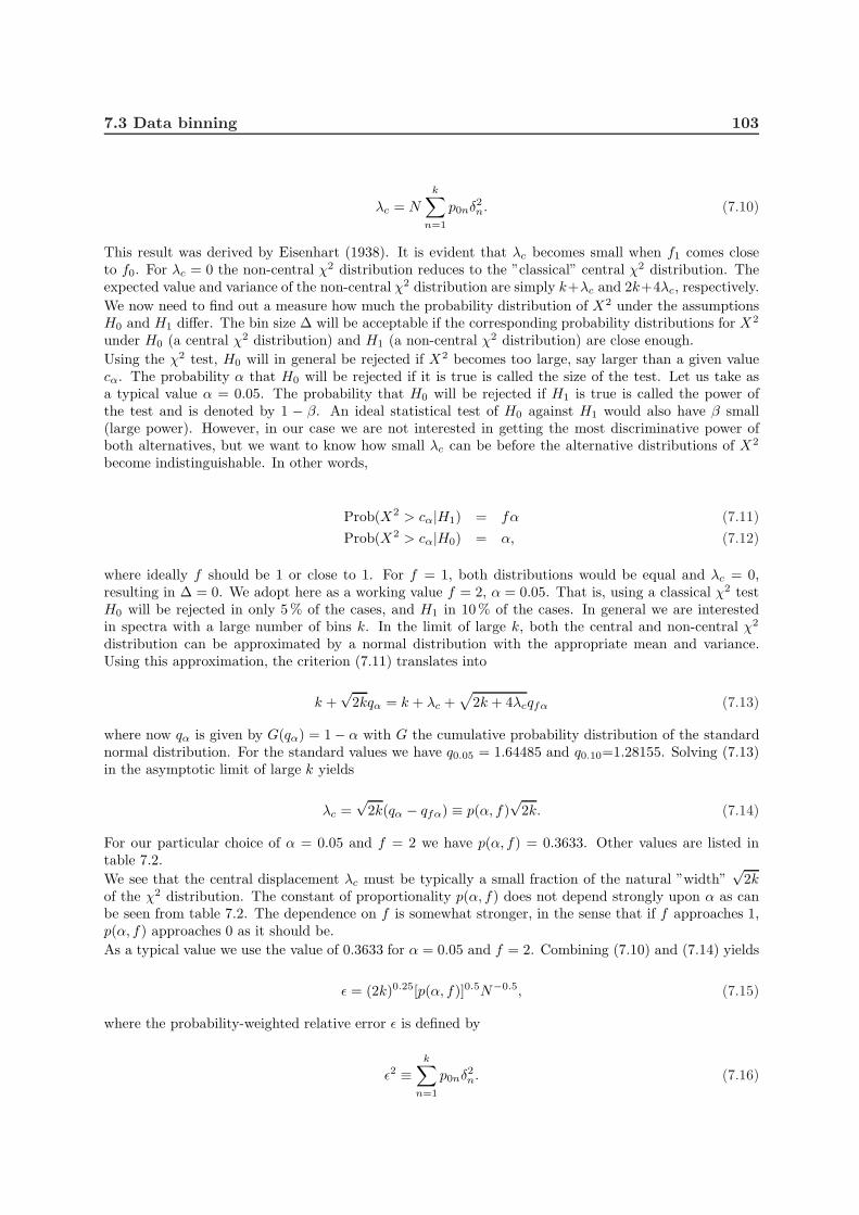
7.3 Data binning 103
λc = N
k∑
n=1
p0nδ2n. (7.10)
This result was derived by Eisenhart (1938). It is evident that λc becomes small when f1 comes closeto f0. For λc = 0 the non-central χ2 distribution reduces to the ”classical” central χ2 distribution. Theexpected value and variance of the non-central χ2 distribution are simply k+λc and 2k+4λc, respectively.
We now need to find out a measure how much the probability distribution of X2 under the assumptionsH0 and H1 differ. The bin size ∆ will be acceptable if the corresponding probability distributions for X2
under H0 (a central χ2 distribution) and H1 (a non-central χ2 distribution) are close enough.
Using the χ2 test, H0 will in general be rejected if X2 becomes too large, say larger than a given valuecα. The probability α that H0 will be rejected if it is true is called the size of the test. Let us take asa typical value α = 0.05. The probability that H0 will be rejected if H1 is true is called the power ofthe test and is denoted by 1 − β. An ideal statistical test of H0 against H1 would also have β small(large power). However, in our case we are not interested in getting the most discriminative power ofboth alternatives, but we want to know how small λc can be before the alternative distributions of X2
become indistinguishable. In other words,
Prob(X2 > cα|H1) = fα (7.11)
Prob(X2 > cα|H0) = α, (7.12)
where ideally f should be 1 or close to 1. For f = 1, both distributions would be equal and λc = 0,resulting in ∆ = 0. We adopt here as a working value f = 2, α = 0.05. That is, using a classical χ2 testH0 will be rejected in only 5% of the cases, and H1 in 10% of the cases. In general we are interestedin spectra with a large number of bins k. In the limit of large k, both the central and non-central χ2
distribution can be approximated by a normal distribution with the appropriate mean and variance.Using this approximation, the criterion (7.11) translates into
k +√
2kqα = k + λc +√
2k + 4λcqfα (7.13)
where now qα is given by G(qα) = 1 − α with G the cumulative probability distribution of the standardnormal distribution. For the standard values we have q0.05 = 1.64485 and q0.10=1.28155. Solving (7.13)in the asymptotic limit of large k yields
λc =√
2k(qα − qfα) ≡ p(α, f)√
2k. (7.14)
For our particular choice of α = 0.05 and f = 2 we have p(α, f) = 0.3633. Other values are listed intable 7.2.
We see that the central displacement λc must be typically a small fraction of the natural ”width”√
2kof the χ2 distribution. The constant of proportionality p(α, f) does not depend strongly upon α as canbe seen from table 7.2. The dependence on f is somewhat stronger, in the sense that if f approaches 1,p(α, f) approaches 0 as it should be.
As a typical value we use the value of 0.3633 for α = 0.05 and f = 2. Combining (7.10) and (7.14) yields
ǫ = (2k)0.25[p(α, f)]0.5N−0.5, (7.15)
where the probability-weighted relative error ǫ is defined by
ǫ2 ≡k
∑
n=1
p0nδ2n. (7.16)

104 Response matrices
Table 7.2: Scaling factors for the displacement parameter
α f p(α, f)
0.01 2.0 0.272600.025 2.0 0.315110.05 2.0 0.363300.10 2.0 0.47513
0.05 1.2 0.090080.05 1.5 0.205320.05 2.0 0.36330
7.3.5 Extension to complex spectra
The χ2 test and the estimates that we derived hold for any spectrum. In (7.15) N should represent thetotal number of counts in the spectrum and k the total number of bins. Given a spectrum with pdff0(x), and adopting a certain bin width ∆, the Shannon approximation f1(x) can be determined, andaccordingly the value of ǫ2 can be obtained from (7.16). By using (7.15) the value of N corresponding to∆ is found, and by inverting this relation, the bin width as a function of N is obtained.
This method is not always practical, however. First, for many X-ray detectors the spectral resolution isa function of the energy, hence binning with a uniform bin width over the entire spectrum is not alwaysdesired.
Another disadvantage is that regions of the spectrum with good statistics are treated the same way asregions with poor statistics. Regions with poor statistics contain less information than regions with goodstatistics, hence can be sampled on a much coarser grid.
Finally, a spectrum often extends over a much wider energy band than the spectral resolution of thedetector. In order to estimate ǫ2, this would require that first the model spectrum, convolved with theinstrument response, should be used in order to determine f0(x). However, the true model spectrum isknown in general only after spectral fitting. The spectral fitting can be done only after a bin size ∆ hasbeen set.
It is much easier to characterize the errors in the line-spread function of the instrument for a given bin size∆, since that can be done independently of the incoming photon spectrum. If we restrict our attentionnow to a region r of the spectrum with a width of the order of a resolution element, then in this regionthe observed spectrum is mainly determined by the convolution of the lsf in this resolution element rwith the true model spectrum in a region with a width of the order of the size of the resolution element.We ignore here any substantial tails in the lsf, since they are of little importance in the determination ofthe optimum bin size/resolution.
If all photons within the resolution element would be emitted at the same energy, the observed spectrumwould be simply the lsf multiplied by the number of photons Nr. For this situation, we can easilyevaluate ǫ2r for a given binning. If the spectrum is not mono-energetic, then the observed spectrum is theconvolution of the lsf with the photon distribution within the resolution element, and hence any samplingerrors in the lsf will be more smooth (smaller) than in the mono-energetic case. It follows that if wedetermine ǫ2r from the lsf, this is an upper limit to the true value for ǫ2 within the resolution element r.
In (7.10) the contribution to λc for all bins is added. The contribution of a resolution element r to thetotal is then given by Nrǫ
2r, where Nr must be the number of photons in the resolution element. We keep
here as a working definition of a resolution element the size of a region with a width equal to the FWHMof the instrument. An upper limit to Nr can be obtained by counting the number of events within oneFWHM and multiplying it by the ratio of the total area under the lsf (should be equal to 1) to the areaunder the lsf within one FWHM (should be smaller than 1).
We now demand that the contribution to λc from all resolution elements is the same. Accordingly,resolution elements with many counts need to have f1 closer to f0 than regions with less counts.
If there are R resolution elements in the spectrum, we demand therefore for each resolution element r

7.3 Data binning 105
the following condition:
λc,r ≡ Nrǫ2r = λc/R (7.17)
with
ǫ2r ≡kr∑
n=1
p0nδ2n, (7.18)
where now p0n and δn are related to the lsf, not to the observed spectrum.Further kr is the number of bins within the resolution element. The value of λc in (7.17) is given againby (7.14) where now k represents the total number of bins in the spectrum, i.e.
k =R
∑
r=1
kr. (7.19)
Combining everything, we have for each resolution element r:
ǫr = (2k)0.25[p(α, f)]0.5(RNr)−0.5 (7.20)
7.3.6 Difficulties with the χ2 test
The first step in applying the theory derived above is evaluating (7.18) for a given lsf. Let us take aGaussian lsf, sampled with a step size of 1σ as an example. Table 7.3 summarizes the intermediate steps.
Table 7.3: Contribution to λc,r for a gaussian lsf
n p0n p1n p0n − p1n p0nδ2n
-8 6.11 10−16 3.04 10−4 -3.04 10−4 1.51 108
-7 1.28 10−12 -3.33 10−4 3.33 10−4 8.65 104
-6 9.85 10−10 3.65 10−4 -3.65 10−4 1.35 102
-5 2.86 10−7 -3.99 10−4 3.99 10−4 5.57 10−1
-4 3.14 10−5 4.60 10−4 -4.29 10−4 5.86 10−3
-3 1.32 10−3 8.77 10−4 4.41 10−4 1.48 10−4
-2 2.14 10−2 2.18 10−2 -4.10 10−4 7.85 10−6
-1 1.36 10−1 1.36 10−1 3.04 10−4 6.78 10−7
0 3.41 10−1 3.42 10−1 -1.14 10−4 3.80 10−8
1 3.41 10−1 3.42 10−1 -1.14 10−4 3.80 10−8
2 1.36 10−1 1.36 10−1 3.04 10−4 6.78 10−7
3 2.14 10−2 2.18 10−2 -4.10 10−4 7.85 10−6
4 1.32 10−3 8.77 10−4 4.41 10−4 1.48 10−4
5 3.14 10−5 4.60 10−4 -4.29 10−4 5.86 10−3
6 2.86 10−7 -3.99 10−4 3.99 10−4 5.57 10−1
7 9.85 10−10 3.65 10−4 -3.65 10−4 1.35 102
8 1.28 10−12 -3.33 10−4 3.33 10−4 8.65 104
It is seen immediately that for large values of |n|, the probability p0n of a photon falling in bin ndecreases rapidly. Also, the approximation is always better than 0.0005. However, the relative error ofthe approximation increases as n increases. Therefore, the largest contribution to χ2 comes from thetails of the Gaussian distribution! In practice one could circumvent this by cutting the summation atsome finite n. It is well known that for the χ2 test to be valid, the expected number of events in eachbin should not be too small. The summation could be stopped where Nrp0n becomes a few. However,

106 Response matrices
since the largest contribution to ǫ2r comes from the largest value of |n|, the value of ǫ2r will be a very steepfunction of the precise cut-off criterion, which is an undesirable effect.An alternative solution can be obtained by using the Kolmogorov-Smirnov test, which is elaborated inthe following section.
7.3.7 The Kolmogorov-Smirnov test
Table 7.4: Maximum difference dn for a gaussian lsf
n p0n dn
-8 6.106 10−16 1.586 10−4
-7 1.279 10−12 -1.740 10−4
-6 9.853 10−10 1.909 10−4
-5 2.857 10−7 -2.079 10−4
-4 3.138 10−5 2.209 10−4
-3 1.318 10−3 -2.202 10−4
-2 2.140 10−2 1.896 10−4
-1 1.359 10−1 -1.139 10−4
0 3.413 10−1 2.675 10−9
1 3.413 10−1 1.139 10−4
2 1.359 10−1 -1.896 10−4
3 2.140 10−2 2.202 10−4
4 1.318 10−3 -2.209 10−4
5 3.138 10−5 2.079 10−4
6 2.857 10−7 -1.909 10−4
7 9.853 10−10 1.740 10−4
8 1.279 10−12 -1.586 10−4
A good alternative to the χ2 test for the comparison of probability distributions is the Kolmogorov-Smirnov test. This powerful, non-parametric test is based upon the test statistic D given by
D = max |S(x) − F (x)|, (7.21)
where S(x) is the observed cumulative distribution for the sample of size N . Clearly, if D is large F (x)is a bad representation of the observed data set. The statistic D′ ≡
√ND for large N (typically 10
or larger) has the limiting Kolmogorov-Smirnov distribution. The hypothesis that the true cumulativedistribution is F will be rejected if D′ > cα, where the critical value cα corresponds to a certain size α ofthe test. A few values for the confidence level are given in table 7.5. The expected value of the statisticD′ is
√
π/2 ln 2=0.86873, and the standard deviation is π√
1/12− (ln 2)2/π=0.26033.Similar to the case of the χ2 test, we can argue that a good criterion for determining the optimum binsize ∆ is that the maximum difference
λk ≡√N max
m|Fs(m∆) − F (m∆)| (7.22)
should be sufficiently small as compared to the statistical fluctuations described by D′. Similar to (7.11)we can derive equations determining λk for a given size of the test α and f :
FKS(cα) = 1 − α, (7.23)
FKS(cα − λk) = 1 − fα. (7.24)

7.3 Data binning 107
Table 7.5: Critical valuse cα for the Kolmogorov-Smirnov test as a function of the size of thetest α
α cα α cα0.01 1.63 0.27 1.000.05 1.36 0.50 0.830.10 1.22 0.95 0.520.15 1.14 0.98 0.470.20 1.07 0.99 0.44
Equation (7.23) gives the critical value for the Kolmogorov-statistic as a function of the size α, under theassumption H0. Equation (7.24) gives the critical value for the Kolmogorov-statistic as a function of thesize α, under the assumption H1. Taking α = 0.05 and f = 2, we find λk = 0.134. Again, as in the caseof the χ2 test, this quantity depends only weakly upon α: for α = 0.01, f = 2 we would have λ = 0.110.
Similar for the case of the χ2 test, we now change our focus to the case of multiple resolution elements.Suppose that in each of the R resolution elements we perform a Kolmogorov-Smirnov test. How can wecombine the tests in the different regions? For the χ2 test we could simply add the contributions fromthe different regions. For the Kolmogorov-Smirnov test it is more natural to test for the maximum δ:
δ ≡ maxr
√
NrDr, (7.25)
where as before Nr is the number of photons in the resolution element r, and Dr is given by (7.21)over the interval r. Note that the integral of Sr(x) and Fr(x) over the interval r should be 1. Ourtest statistic therefore combines ”normalized” KS-tests over each resolution element. All the
√NrDr
are independently distributed according to a KS distribution, hence the cumulative distribution functionfor their maximum is simply the Rth power of a single stochastic variable with the KS distribution.Therefore we obtain instead of (7.23, 7.24):
FKS(cα)R = 1 − α, (7.26)
FKS(cα − λk)R = 1 − fα. (7.27)
The hypothesis H0 is rejected if δ > cα. For our choice of α = 0.05 and f = 2 we can calculate λk as afunction of R by solving numerically the above equations using the exact Kolmogorov-Smirnov cumulativeprobability distribution function. In fig. 7.1 we show the solution. It is seen that it depends only weaklyupon R; it has a maximum value 0.134 at R = 1 and is less than 3 times smaller at R = 1010. We canapproximate λk as a function of R by the following polynomial:
λk(R) =5
∑
i=0
ai(10 log(R)
10)i, (7.28)
where the numbers ai are given in table 7.6. Note the factor of 10 in the denominator! The rms deviationof the approximation is less then 10−4. The corresponding value for cα is plotted in fig. 7.2, and isapproximated with an rms deviation of 0.0004 by the polynomial:
cα(R) =5
∑
i=0
bi(10 log(R)
10)i, (7.29)
where the numbers bi are given in table 7.6. This approximation is only valid for the range 0.5 < R < 1010.

108 Response matrices
Figure 7.1: Displacement λk as a function of the number of resolution elements R. A polynomialapproximation is given in the text.
Figure 7.2: Critical value cα as a function of the number of resolution elements R. A polynomialapproximation is given in the text.
7.3.8 Examples
Let us apply the theory derived before to some specific line spread functions. First we consider a Cauchy(or Lorentz) distribution, given by

7.3 Data binning 109
Table 7.6: Coefficients for the approximations for λk and cα
i ai bi0 0.1342 1.35961 -0.3388 4.06092 0.7994 -4.35223 -1.1697 5.22254 0.9053 -3.78815 -0.2811 1.1491
f(x) =a
π(a2 + x2), (7.30)
where a is the width parameter. The FWHM equals 2a. Next we consider the Gaussian distribution,given by
f(x) =1√2πσ
e−x2/2σ2
, (7.31)
with σ the standard deviation. The FWHM is given by√
ln 256σ, which is approximately 2.3548σ.We have computed the value for δ ≡ λk/
√N numerically for both distributions. We have taken into
account also the effect of possible phase shifts, i.e. that the center of the distribution does not coincidewith a grid point but with a certain phase of the grid. The maximum bin width ∆/FWHM as a functionof the maximum absolute difference δ between the true and approximated cumulative density distributionis plotted for both distributions in fig. 7.3.
Figure 7.3: Required bin width ∆ as a function of the accuracy parameter δ for a Gaussiandistribution (solid line) and a Cauchy distribution (dashed line).
We can approximate both curves with sufficient accuracy by a polynomial in x ≡10 log δ as
10 log(∆/FWHM) =
4∑
i=0
ci(10 log(δ)
10)i, (7.32)
10 log(∆/FWHM) =
4∑
i=0
gi(10 log(δ)
10)i, (7.33)

110 Response matrices
for the Cauchy distribution (7.32) and Gaussian distribution (7.33) respectively, with the coefficents givenin table 7.7.
Table 7.7: Coefficients for the approximations for the Cauchy and Gauss distribution.
i ci gi
0 0.400 0.2771 5.065 3.8632 9.321 8.4703 9.333 9.4964 3.584 3.998
The rms deviation of these fits over the range 10−9 < δ < 1 is 0.0086 for the Cauchy distribution and0.0070 for the Gauss distribution. Outside of this range the approximation gets worse, however thosevalues for δ are of no practical use.The bin size as a function of the number of resolution elements R and number of photons per resolutionelement Nr is now obtained by combining (7.32) or (7.33) with (7.28) and using
λk =√
Nrδ. (7.34)
Figure 7.4: Required bin width ∆ relative to the FWHM for a Gaussian distribution as a functionof Nr for R=1, 10, 100, 1000 and 10000 from top to bottom, respectively.
In fig. 7.4 we show the required binning, expressed in FWHM units, for a Gaussian lsf as a function of Rand Nr, and in fig. 7.5 for a Lorentzian.For the Gaussian, the resolution depends only weakly upon the number of counts Nr. However in the caseof a pure Lorentzian profile, the required bin width is somewhat smaller than for a Gaussian. This is dueto the fact that the Fourier transform of the Lorentzian has relatively more power at high frequencies thana Gaussian (exp [−ωσ] versus exp
[
−(ωσ)2/2]
respectively). For low count rate parts of the spectrum,the binning rule 1/3 FWHM usually is too conservative!
7.3.9 Final remarks
We have estimated conservative upper bounds for the required data bin size. In the case of multipleresolution elements, we have determined the bounds for the worst case phase of the grid with respect tothe data. In practice, it is not likely that all resolution elements would have the worst possible alignment.In fact, for the Gaussian lsf, the phase-averaged value for δ at a given bin size ∆ is always smaller than

7.4 Model binning 111
Figure 7.5: Required bin width ∆ relative to the FWHM for a Lorentz distribution as a functionof Nr for R=1, 10, 100, 1000 and 10000 from top to bottom, respectively.
0.83, and is between 0.82–0.83 for all values of ∆/FWHM < 1.3. However we recommend to use theconservative upper limits as given by (7.33).
Another issue is the determination of Nr, the number of events within the resolution element. We haveargued that an upper limit to Nr can be obtained by counting the number of events within one FWHMand multiplying it by the ratio of the total area under the lsf (should be equal to 1) to the area underthe lsf within one FWHM (should be smaller than 1). For the Gaussian lsf this ratio equals 1.314, forother lsfs it is better to determine it numerically, and not to use the Gaussian value 1.314.
Finally, in some cases the lsf may contain more than one component. For example, the grating spectraobtained with the EUVE SW, MW and LW detector have first, second, third etc. order contributions.Other instruments have escape peaks or fluorescent contributions. In general it is advisable to determinethe bin size for each of these components individually, and simply take the smallest bin size as the finalone.
7.4 Model binning
7.4.1 Model energy grid
The spectrum of any X-ray source is given by its photon spectrum f(E). f(E) is a function of thecontinuous variable E, the photon energy, and has e.g. units of photons m−2 s−1 keV−1. When wereconstruct how this source spectrum f(E) is observed by an instrument, f(E) is convolved with theinstrument response R(c, E) in order to produce the observed count spectrum s(c) as follows:
s(c) =
∫
R(c, E)f(E)dE (7.35)
where the variable c denotes the ”observed” (see below) photon energy and s has units of counts s−1 keV−1.The response function has the dimensions of an (effective) area, and can be given in e.g. m2.
The variable c was denoted as the ”observed” photon energy, but in practice it is some electronic signalin the detector used, the strength of which usually cannot take arbitrary values, but can have only alimited set of discrete values. A good example of this is the pulse-height channel for a CCD detector.
In almost all circumstances it is not possible to do the integration in eqn. (7.35) analytically, due tothe complexity of both the model spectrum and the instrument response. For that reason, the modelspectrum is evaluated at a limited set of energies, corresponding to the same pre-defined set of energiesthat is used for the instrument response R(c, E). Then the integration in eqn. (7.35) is replaced by asummation. We call this limited set of energies the model energy grid or shortly the model grid. For each

112 Response matrices
bin j of this model grid we define a lower and upper bin boundary E1j and E2j as well as a bin centroidEj and a bin width ∆Ej , where of course Ej is the average of E1j and E2j , and ∆Ej = E2j - E1j .Provided that the bin size of the model energy bins is sufficiently smaller than the spectral resolutionof the instrument, the summation approximation to eqn. (7.35) is in general sufficiently accurate. Theresponse function R(c, E) has therefore been replaced by a response matrix Rij , where the first index idenotes the data channel, and the second index j the model energy bin number.We have explicitly:
Si =∑
j
RijFj , (7.36)
where now Si is the observed count rate in counts/s for data channel i and Fj is the model spectrum(photons m−2 s−1) for model energy bin j.This basic scheme is widely used and has been implemented e.g. in the XSPEC and SPEX (version 1.10and below) packages.
7.4.2 Evaluation of the model spectrum
The model spectrum Fj can be evaluated in two ways. First, the model can be evaluated at the bincentroid Ej , taking essentially
Fj = f(Ej)∆Ej . (7.37)
This is appropriate for smooth continuum models like blackbody radiation, power laws etc. For line-likeemission it is more appropriate to integrate the line flux within the bin analytically, and taking
Fj =
E2j∫
E1j
f(E)dE. (7.38)
Now a sometimes serious flaw occurs in most spectral analysis codes. The observed count spectrum Si
is evaluated straightforward using eqn. (7.36). Hereby it is assumed that all photons in the model bin jhave exactly the energy Ej . This has to be done since all information on the energy distribution withinthe bin is lost and Fj is essentially only the total number of photons in the bin. Why is this a problem?It should not be a problem if the model bin width ∆Ej is sufficiently small. However, this is (most often)not the case.Let us take an example. The standard response matrix for the ASCA SIS detector uses a uniformmodel grid with a bin size of 10 eV. At a photon energy of 1 keV, the spectral resolution (FWHM) ofthe instrument is about 50 eV, hence the line centroid of an isolated narrow line feature containing Ncounts can be determined with a statistical uncertainty of 50/2.35
√N eV (we assumed here for simplicity
a Gaussian instrument response, for which the FWHM is approximately 2.35σ). Thus, for a moderatelystrong line of say 400 counts, the line centroid can be determined in principle with an accuracy of 1 eV,ten times better than the step size of the model energy grid. If the true line centroid is close to theboundary of the energy bin, there is a mis-match (shift) of 5 eV between the observed count spectrumand the predicted count spectrum, at about the 5σ significance level! If there are more of these lines inthe spectrum, it is not excluded that never a satisfactory fit (in a χ2 sense) is obtained, even in thosecases where we know the true source spectrum and have a perfectly calibrated instrument! The problembecomes even more worrysome if e.g. detailed line-centroiding is done in order to derive velocity fields,like has been done e.g. for the Cas A supernova remnant.A simple way to resolve these problems is just to increase the number of model bins. This robust methodalways works, but at the expense of a lot of computing time. For CCD-resolution spectra this is perhapsnot a problem, but with the increased spectral resolution and sensitivity of the grating spectrometers ofAXAF and XMM this becomes cumbersome.For example, with a spectral resolution of 0.04 A over the 5–38 A band, the RGS detector of XMM willhave a bandwidth of 825 resolution elements, which for a Gaussian response function translates into 1940

7.4 Model binning 113
times σ. Several of the strongest sources to be observed by this instrument will have more than 10000counts in the strongest spectral lines (example: Capella), and this makes it necessary to have a modelenergy grid bin size of about σ/
√
(10000). The total number of model bins is then 194 000.
Most of the computing time in thermal plasma models stems from the evaluation of the continuum. Thereason is that e.g. the recombination continuum has to be evaluated for all energies, for all relevantions and for all relevant electronic subshells of each ion. On the other hand, the line power needs to beevaluated only once for each line, regardless of the number of energy bins. Therefore the computing timeis approximately proportional to the number of bins. Going from ASCA-SIS resolution (1180 bins) toRGS resolution (194 000 bins) therefore implies more than a factor of 160 increase in computer time. Andthen it can be anticipated that due to the higher spectral resolution of the RGS more complex spectralmodels are needed in order to explain the observed spectra than are needed for ASCA, with more freeparameters, which also leads to additional computing time. And finally, the response matrices of the RGSbecome extremely large. The RGS spectral response is approximately Gaussian in its core, but containsextended scattering wings due to the gratings, up to a distance of 0.5 A from the line center. Therefore,for each energy the response matrix is significantly non-zero for at least some 100 data channels, givingrise to a response matrix of 20 million non-zero elements. In this way the convolution of the modelspectrum with the instrument response becomes also a heavy burden.
For the AXAF-LETG grating the situation is even worse, given the wider energy range of that instrumentas compared to the XMM-RGS.
Fortunately there are more sophisticated ways to evaluate the spectrum and convolve it with the instru-ment response, as is shown in the next subsection.
7.4.3 Binning the model spectrum
We have seen in the previous subsection that the ”classical” way to evaluate model spectra is to calculatethe total number of photons in each model energy bin, and to act as if all flux is at the center of thebin. In practice, this implies that the ”true” spectrum f(E) within the bin is replaced by its zeroth orderapproximation f0(E), given by
f0(E) = Nδ(E − Ej), (7.39)
where N is the total number of photons in the bin, Ej the bin centroid as defined in the previous sectionand δ is the delta-function.
In this section we assume for simplicity that the instrument response is Gaussian, centered at the truephoton energy and with a standard deviation σ. Many instruments have line spread functions withGaussian cores. For instrument responses with extended wings (e.g. a Lorentz profile) the model binningis a less important problem, since in the wings all spectral details are washed out, and only the lsf coreis important. For a Gaussian profile, the FWHM of the lsf is given by
FWHM =√
ln(256)σ ≃ 2.35σ. (7.40)
How can we measure the error introduced by using the approximation (7.39)? Here we will comparethe cumulative probability distribution function (cdf) of the true bin spectrum, convolved with theinstrumental lsf, with the cdf of the approximation (7.39) convolved with the instrumental lsf. Thecomparison is done using a Kolmogorov-Smirnov test, which is amongst the most powerful tests indetecting the difference between probability distributions, and which we used successfully in the sectionon data binning. We denote the lsf-convolved cdf of the true spectrum by φ(c) and that of f0 by φ0(c).By definition, φ(−∞) = 0 and φ(∞) = 1, and similar for φ0.
Similar to section 7.3, we denote the maximum absolute difference between φ and φ0 by δ. Again,λk ≡
√Nδ should be kept sufficently small as compared to the expected statistical fluctuations
√ND,
where D is given again by eqn. (7.21). Following section 7.3 further, we divide the entire energy rangeinto R resolution elements, in each of which a KS test is performed. For each of the resolution elements,we determine the maximum value for λk from (7.26)–(7.28), and using (7.34) we find for a given numberof photons Nr in the resolution element the maximum allowed value for δ in the same resolution element.

114 Response matrices
The approximation f0 to the true distribution f as given by eqn. (7.39) fails most seriously in the casethat the true spectrum within the bin is also a δ-function, but located at the bin boundary, at a distance∆E/2 from the assumed line center at the bin center.Using the Gaussian lsf, it is easy to show that the maximum error δ0 for f0 to be used in the Kolmogorov-Smirnov test is given by
δ0 =1
2√
2π(∆E
σ) (7.41)
This approximation holds in the limit of ∆E ≪ σ. Inserting eqn. (7.40) we find that the bin size shouldbe smaller than
∆E
FWHM< 2.1289 λ(R)N−0.5. (7.42)
Figure 7.6: Maximum model energy grid bin width ∆E in terms of the FWHM as a function ofthe number of photons Nr in the bin, using different approximations f0 (solid line), f1 (dashedline) and f2 (dotted line) as discussed in the text. The calculation is done for R = 1 (uppercurves) or R = 1000 (lower curves) resolution elements.
Exact numerical results are shown in fig. 7.6. The approximation (7.41) is a lower limit to the exactresults, so can be safely used. A somewhat better approximation (but still a lower limit) appears to bethe following:
∆E
FWHM= 2.129δ0 − 0.004δ20 + 0.555δ30. (7.43)
As expected, one sees that for N = 10000 one needs to bin the model spectrum by about 0.01 times theFWHM.A further refinement can be reached as follows. Instead of putting all photons at the bin center, we canput them at their average energy. This first-order approximation can be written as
f1(E) = Nδ(E − Ea), (7.44)
where Ea is given by
Ea =
E2j∫
E1j
f(E)EdE (7.45)
In the worst case for approximation f0 (namely a narrow line at the bin boundary) the approximationf1 yields exact results. In fact, it is easy to see that the worst case for f1 is a situation with two δ-lines

7.4 Model binning 115
of equal strength, one at each bin boundary. In that case the width of the resulting count spectrum φ1
will be broader than σ. Again in the limit of small ∆E, it is easy to show that the maximum error δ1for f1 to be used in the Kolmogorov-Smirnov test is given by
δ1 =1
8√
2πe(∆E
σ)2 (7.46)
where e is the base of the natural logarithms. Accordingly, the limiting bin size for f1 is given by
∆E
FWHM< 2.4418 λ(R)0.5N−0.25. (7.47)
Exact results are plotted again in fig. 7.6. The better numerical approximation is
∆E
FWHM= 2.44δ0.5
1 − 0.05δ1 + 1.95δ1.51 . (7.48)
It is seen immediately that for large N the approximation f1 requires a significantly smaller number ofbins than f0.We can improve further by not only calculating the average energy of the photons in the bin (the firstmoment of the photon distribution), but also its variance (the second moment).In this case we approximate
f2(E) = N exp[(E − Ea)/2τ2)], (7.49)
where τ is given by
τ =
E2j∫
E1j
f(E)(E − Ea)2dE (7.50)
The resulting count spectrum is then simply Gaussian, with the average value centered at Ea and thewidth slightly larger than the instrumental width σ, namely
√σ2 + τ2.
The worst case for f0 again occurs for two δ-lines at the opposite bin boundaries, but now with unequalstrength. It can be shown again in the small bin width limit that
δ2 =1
36√
6π(∆E
σ)3 (7.51)
and that this maximum occurs for a line ratio of 6√
3 − 1. The limiting bin size for f2 is given by
∆E
FWHM< 2.2875 λ(R)1/3N−1/6. (7.52)
Exact results are plotted again in fig. 7.6. The better numerical approximation is
∆E
FWHM= 2.29δ
1/32 − 0.11δ
2/32 + 2.72δ2. (7.53)
7.4.4 Which approximation to choose?
It is now time to compare the different approximations f0, f1 and f2 as derived in the previous subsection.It can be seen from fig. 7.6 that the approximation f1 implies an order of magnitude or more improvementover the classical approximation f0. However, the approximation f2 is only slightly better than f1.Moreover, the computational burden of approximation f2 is large. The evaluation of (7.50) is ratherstraightforward to do, although care should be taken with single machine precision: first the averageenergy Ea should be determined, and then this value should be used in the estimation of τ . A moreserious problem is that the width of the lsf should be adjusted from σ to
√σ2 + τ2. If the lsf is a pure
Gaussian, this can be done analytically; however for a slightly non-Gaussian lsf the true lsf should beconvolved in general numerically with a Gaussian of width τ in order to obtain the effective lsf for the

116 Response matrices
particular bin, and the computational burden is quite heavy. On the other hand, for f1 only a shift inthe lsf is sufficient.Therefore we recommend here to use the linear approximation f1. The optimum bin size is thus givenby (7.28), (7.34) and (7.48).
7.4.5 The effective area
In the previous subsection we have seen how the optimum model energy grid can be determined, takinginto account the possible presence of narrow spectral features, the number of resolution elements andthe flux of the source. There remains one other factor to be taken into account, and that is the energydependence of the effective area. In the previous section we have considered merely the effect of thespectral redistribution (”rmf” in XSPEC terms), here we consider the ”arf”.If the effective area Aj(E) would be a constant Aj for a given model bin j, and if the photon flux of thebin in photonsm−2 s−1 would be given by Fj , then the total count rate produced by this bin would besimply AjFj . This approach is actually used in the ”classical” way of analysing spectra, and it is justifiedin the approximation that all photons of the model bin would have the energy of the bin centroid. Thisis not always the case, however, and in the previous subsection we have given arguments that it is betternot only to take into account the flux Fj but also the average energy Ea of the photons within the modelbin. This average energy Ea is in general not equal to the bin centroid Ej , and hence we need to evaluatethe effective area not at Ej but at Ea.In general the effective area is energy-dependent and it is not trivial that the constant approximationover the width of a model bin is justified. In several cases this will not be the case. We consider herethe most natural first-order extension, namely the assumption that the effective area within a model binis a linear function of the energy. For each model bin j, we write the effective area A(E) in general asfollows:
Aj(E) = A0j +A1j(E − Ej) + ǫj(E). (7.54)
The above approximation is good when the residuals ǫj(E) are sufficiently small. We use a Taylorexpansion in order to estimate the residuals:
ǫj(E) ≈ 1
2A′′(Ej)(E − Ej)
2, (7.55)
where as usual A′′ denotes the second derivative of A with respect to the energy. It is immediately seenfrom the above expressions that the maximum error occurs when E is at one of the bin boundaries. Asa consequence, we can estimate the maximum error ǫmax as:
ǫmax =1
8(∆E)2A′′(Ej). (7.56)
By using the approximation (7.54) with ǫ neglected we therefore make at most a maximum error givenby (7.56) in the effective area. This can be translated directly into an error in the predicted count rateby multiplying ǫmax by the photon flux Fj . Alternatively, dividing ǫmax by the effective area A0j at thebin center, we get the maximum error in the predicted probability distribution for the resulting counts.This maximum can be taken also as the maximum deviation δ in the cumulative distribution functionthat we used in the previous sections in the framework of the Kolmogorov-Smirnov tests.Hence we write
δ =(∆E)2A′′(Ej)
8A0j. (7.57)
Using the same theory as in the previous section, we find an expression for the optimum bin size, as faras the effective area is treated in the linear approximation (compare with eqn. (7.47)):
∆E
FWHM<
( 8A
E2jA
′′
)0.5( Ej
FWHM
)
λ(R)0.5N−0.25. (7.58)

7.5 The proposed response matrix 117
The bin width constraint derived here depends upon the dimensionless curvature of the effective areaA/E2
jA′′. In most parts of the energy range this will be a number of order unity or less. Since the
second prefactor Ej/FWHM is by definition the resolution of the instrument, we see by comparing (7.58)with (7.47) that in general (7.47) gives the most severe constraint upon the bin width, unless either theresolution gets small (what happens e.g. for the Rosat PSPC detector at low energies), or the effectivearea curvature gets large (what may happen e.g. near the exponential cut-offs caused by filters).Large effective area curvature due to the presence of exponential cut-offs is usually not a very seriousproblem, since these cut-offs also cause the count rate to be very low and hence weaken the binningrequirements. Of course, discrete edges in the effective area should always be avoided in the sence thatedges should always coincide with bin boundaries.In practice, it is a little complicated to estimate from e.g. a look-up table of the effective area its curvature,although this is not impossible. As a simplification for order of magnitude estimates we can use the casewhere A(E) = A0e
bE locally, which after differentiation yields
√
8A
E2jA
′′=
√8
d lnE
d lnA. (7.59)
Inserting this into (7.58), we obtain
∆E
FWHM<
√8(d lnE
d lnA
)( Ej
FWHM
)
λ(R)0.5N−0.25. (7.60)
7.4.6 Final remarks
In the previous two subsections we have given the constraints for determining the optimal model energygrid. Combining both requirements (7.48) and (7.60) we obtain the following optimum bin size:
∆E
FWHM=
11
w1
+ 1wa
(7.61)
where w1 and wa are the values of ∆E/FWHM as calculated using (7.48) and (7.60), respectively.This choice of model binning ensures that no significant errors are made either due to inaccuracies in themodel or effective area for flux distributions within the model bins that have Ea 6= Ej .
7.5 The proposed response matrix
7.5.1 Dividing the response into components
When a response matrix is stored on disk, usually only the non-zero matrix elements are stored andused. This is done in order to save both disk space and computational time. The procedure as used inXSPEC and the older versions of SPEX is then that for each model energy bin j the relevant column ofthe response matrix is subdivided into groups. The groups are the continuous pieces of the column wherethe response is non-zero. In general these groups are stored in a specific order: starting from the lowestenergy, all groups of a single energy are given before turning to the next higher photon energy.This is not the optimal situation neither with respect to disk storage nor with respect to computationalefficiency, as is illustrated by the following example. For the XMM/RGS, the response consists of a narrowgaussian-like core with in addition a broad scattering component due to the gratings. The FWHM ofthe scattering component is typically 10 times larger than that of the core of the response. As a result,if the response would be saved as a ”classical” matrix, we would end up with one response group perenergy, namely the combined core and wings response, since these contributions have overlap, namely inthe region of the gaussian-like core. As a result, the response becomes large, being a significant fractionof the product of the total number of model energy bins times the total number of data channels. Thisis not necessary, since the scattering contribution with its ten times larger width needs to be specifiedonly on a model energy grid with ten times fewer bins, as compared to the gaussian-like core. Thus,by separating out the core and the scattering contribution, the total size of the response matrix can be

118 Response matrices
reduced by about a factor of 10! Of course, as a consequence each contribution needs to carry its ownmodel energy grid with it.
Therefore I propose here to subdivide the response matrix into its physical components. Then for eachresponse component, the optimum model energy grid can be determined according to the methods de-scribed in section 3, and this model energy grid for the component can be stored together with theresponse matrix part of that component. Furthermore, at any energy each component may have at most1 response group. If there would be more response groups, the component should be sub-divided further.
In X-ray detectors other than the RGS detector the subdivision could be quite different. For example,with the ASCA SIS detector one could split up the response e.g. into 4 components: the main diagonal,the Si fluorescence line, the escape peak and a broad component due to split events.
7.5.2 More complex situations
Outline of the problem
In most cases an observer will analyze the data of a single source, with a single spectrum and responsefor a single instrument. However, more complicated situations may arise. Examples are:
1. An extended source, where the spectrum may be extracted from different regions of the detector,but where these spectra need to be analysed simultaneously due to the overlap in point-spreadfunction from one region to the other. This situation is e.g. encountered in the analysis of clusterdata with ASCA or BeppoSAX.
2. For the RGS of XMM, the actual data-space in the dispersion direction is actually two-dimensional:the position z where a photon lands on the detector and its energy or pulse height c as measuredwith the CCD detector. X-ray sources that are extended in the direction of the dispersion axis φare characterised by spectra that are a function of both the energy E and off-axis angle φ. Thesky photon distribution as a function of (φ,E) is then mapped onto the (z, c)-plane. By definingappropriate regions in both planes and evaluating the correct (overlapping) responses, one mayanalyse extended sources.
3. One may also fit simultaneously several time-dependent spectra using the same response, e.g. dataobtained during a stellar flare.
It is relatively easy to model all these situations (provided that the instrument is understood sufficiently,of course), as we show below.
Sky sectors
First, the relevant part of the sky is subdivided into sectors, each sector corresponding to a particularregion of the source, for example a circular annulus centered around the core of a cluster, or an arbitrarilyshaped piece of a supernova remnant, etc.
A sector may also be a point-like region on the sky. For example if there is a bright point sourcesuperimposed upon the diffuse emission of the cluster, we can define two sectors: an extended sector forthe cluster emission, and a point-like sector for the point source. Both sectors might even overlap, as thisexample shows!
Another example: the two nearby components of the close binary α Cen observed with the XMM instru-ments, with overlapping psfs of both components. In that case we would have two point-like sky sectors,each sector corresponding to one of the double star’s components.
The model spectrum for each sky sector may and will be different in general. For example, in the case ofan AGN superimposed upon a cluster of galaxies, one might model the spectrum of the point-like AGNsector using a power law, and the spectrum from the surrounding cluster emission using a thermal plasmamodel.

7.5 The proposed response matrix 119
Detector regions
The observed count rate spectra are extracted in practice in different regions of the detector. It isnecessary here to distinguish clearly the (sky) sectors and (detector) regions. A detector region for theXMM EPIC camera would be for example a rectangular box, spanning a certain number of pixels in thex- and y-directions. It may also be a circular or annular extraction region centered around a particularpixel of the detector, or whatever spatial filter is desired. For the XMM RGS it could be a specific”banana” part of the detector-coordinate CCD pulse-height plane (z, c).
Note that the detector regions need not to coincide with the sky sectors, neither should their number to beequal. A good example of this is again the example of an AGN superimposed upon a cluster of galaxies.The sky sector corresponding to the AGN is simply a point, while, for a finite instrumental psf, itsextraction region at the detector is for example a circular region centered around the pixel correspondingto the sky position of the source.
Also, one could observe the same source with a number of different instruments and analyse the datasimultaneously. In this case one would have only one sky sector but more detector regions, namely onefor each participating instrument.
Consequences for the response
In all the cases mentioned above, where there is either more than one sky sector or more than onedetector region involved, it is necessary to generate the response contribution for each combination ofsky sector - detector region. In the spectral analysis, for each sky sector the model photon spectrum iscalculated, and all these model spectra are convolved with the relevant response contributions in order topredict the count spectra for all detector regions. Each response contribution for a sky sector - detectorregion combination itself may consist again of different response components, as outlined in the previoussubsection.
Combining all this, the total response matrix then will consist of a list of components, each componentcorresponding to a particular sky sector and detector region. For example, let us assume that the RGShas two response contributions, one corresponding to the core of the lsf, and the other to the scatteringwings. Let us assume that this instrument observes a triple star where the instrument cannot resolvetwo of the three components. The total response for this configuration then consists of 12 components,namely 3 sky sectors (assuming each star has its own characteristic spectrum) times two detector regions (aspectrum extracted around the two unresolved stars and one around the other star) times two instrumentalcontributions (the lsf core and scattering wings).
7.5.3 A response component
We have shown in the previous section how for the combination of a particular source configuration andinstrumental properties response matrix components can be defined. In this subsection we investigatehow to build such a matrix component.
Let us first return to our discussion on the optimum model energy grid binning. For high-resolutioninstruments the factor Ej/FWHM in (7.60) is by definition large, and hence for most energies the re-quirements for the binning are driven by the model accuracy, not by the effective area accuracy. Onemight ask whether the approximation of a constant effective area within a model bin instead of the linearapproximation (7.54) would not be sufficient in that case. The reason is the following.
In order to acquire the high accuracy, we need to convolve the model spectrum for the bin, approximatedas a δ-function centered around Ea, with the instrument response. In most cases we cannot do thisconvolution analytically, so we have to make approximations. From our expressions for the observedcount spectrum s(c), eqns. 7.35) and (7.36), it can be easily derived that the number of counts or countrate for data channel i is given by
Si =
ci2∫
ci1
dc
∫
dER(c, E)f(E) (7.62)

120 Response matrices
where as before ci1 and ci2 are the formal channel limits for data channel i and Si is the observedcount rate in counts/s for data channel i. Interchanging the order of the integrations and defining themono-energetic response for data channel i by Ri(E) as follows:
Ri(E) ≡ci2∫
ci1
R(c, E)dc, (7.63)
we have
Si =
∫
dEf(E)Ri(E). (7.64)
From the above equation we see that as long as we are interested in the observed count rate Si of a givendata channel i, we get that number by integrating the model spectrum multiplied by the ”effective area”Ri(E) for that particular data channel. We have approximated f(E) for each model bin j by (7.44), sothat (7.64) becomes:
Si =∑
j
FjRi(Ea,j), (7.65)
where as before Ea,j is the average energy of the photons in bin j, given by (7.45) and Fj is the total
photon flux for bin j, in e.g. photonsm−2 s−1. It is seen from (7.65) that we need to evaluate Ri not atthe bin center Ej but at Ea,j , as expected.
Formally we may split-up Ri(E) in an effective area part A(E) and a redistribution part ri(E) in such away that
Ri(E) = A(E)ri(E). (7.66)
We have chosen our binning already in such a way that we have sufficient accuracy when the total effectivearea A(E) within each model energy grid bin j is approximated by a linear function of the photon energyE. Hence the ”arf”-part of Ri is of no concern. We only need to check how the redistribution (”rmf”)part ri can be calculated with sufficiently accuracy.For ri the arguments go exactly the same as for A(E), in the sense that if we approximate it locally foreach bin j by a linear function of energy, the maximum error that we make is proportional to the secondderivative with respect to E of ri, cf. (7.56).In fact, for a Gaussian redistribution function the following is straightforward to proove, and is left hereas an excercise for the reader:
Theorem 1 Assume that for a given model energy bin j all photons are located at the upper bin boundaryEj+∆E/2. Suppose that for all data channels we approximate ri by a linear function of E, the coefficientsbeing the first two terms in the Taylor expansion around the bin center Ej . Then the maximum error δmade in the cumulative count distribution (as a function of the data channel) is given by (7.47) in thelimit of small ∆E.
The importance of the above theorem is that it shows that the binning for the model energy grid thatwe have chosen in section 2 is also sufficiently accurate so that ri(E) can be approximated by a linearfunction of energy within a model energy bin j, for each data channel i. Since we showed already thatour binning is also sufficient for a similar linear approximation to A(E), it follows that also the totalresponse Ri(E) can be approximated by a linear function. Hence we use within the bin j:
Ri(Ea,j) = Ri(Ej) +dRi
dEj(Ej) (Ea,j − Ej). (7.67)
Inserting the above in (7.65) and comparing with (7.36) for the classical response matrix, we obtainfinally:

7.6 Determining the grids in practice 121
Si =∑
j
Rij,0Fj +Rij,1(Ea − Ej)Fj , (7.68)
where Rij,0 is the ”classical” response matrix, evaluated for photons at the bin center (Note: not theaverage over the bin!), and Rij,1 is its derivative with respect to the photon energy (Note: not tobe confused with the data channel!), evaluated also at the bin center. In addition to the ”classical”convolution, we thus get a second term containing the relative offset of the photons with respect to thebin center. This is exactly what we intended to have when we argued that the number of bins could bereduced considerably by just taking that offset into account! It is just at the expense of an additionalderivative matrix, which means only a factor of two more disk space and computation time. But for thisextra expenditure we gained much more disk space and computational efficiency because the number ofmodel bins is reduced by a factor between 10–100!
Finally a practical note. The derivative Rij,1 can be calculated in practice either analytically or bynumerical differentiation. In the last case it is more accurate to evaluate the derivative by taking thedifference at E+∆E/2 and E−∆E/2, and wherever possible not to evaluate it at one of these boundariesand the bin center. This last situation is perhaps only un-avoidable at the first and last energy value.
Also, negative response values should be avoided. Thus it should be ensured that Rij,0 + Rij,1h iseverywhere non-negative for −∆E/2 ≤ h ≤ ∆E/2. This can be translated into the constraint that Rij,1
should be limited always to the following interval:
−2Rij,0/∆E ≤ Rij,1 ≤ 2Rij,0/∆E. (7.69)
Whenever the calculated value of Rij,1 should exceed the above limits, the limiting value should beinserted instead. This situation may happen for example for a Gaussian redistribution for responses afew σ away from the center, where the response falls of exponentially. However, the response Rij,0 issmall anyway for those energies so this limitation is not serious. The only reason is that we want to avoidnegative predicted count rates, whatever small they may be.
7.6 Determining the grids in practice
Based upon the theory developed in the previous sections, I present here a practical set of algorithmsfor the determination of both the optimal data binning and the model energy grid determination. Thismay be helpful for the practical purpose of developing software for a particular instrument in order toconstruct the relevant response matrix.
7.6.1 Creating the data bins
Given an observed spectrum obtained by some instrument, the following steps should be performed inorder to generate an optimally binned spectrum.
1. Determine for each original data channel i the nominal energy Ej0, defined as the energy for whichthe response at channel i reaches its maximum value. In most cases this will be the nominal channelenergy.
2. Determine for each data channel i the limiting points (i1, i2) for the FWHM, in such a way thatRk,j0 ≥ 0.5Ri,j0 for all i1 ≤ k ≤ i2 while the range of (i1, i2) is as broad as possible.
3. By (linear) interpolation, determine for each data channel the points (fractional channel numbers)c1 and c2 near i1 and i2 where the response is actually half its maximum value. By virtue of theprevious step, the absolute difference |c1 − i1| and |c2 − i2| never can exceed 1.
4. Determine for each data channel i the FWHM in number of channels ci, by calculating c2 − c1.Assure that ci is at least 1.

122 Response matrices
5. Determine for each original data channel i the FWHM in energy units (e.g. in keV). Call this Wi.This and the previous steps may of course also be performed directly using instrument calibrationdata.
6. Determine the number of resolution elements R by the following approximation:
R =∑
i
1
ci. (7.70)
7. Determine the parameter λk(R) using (7.28).
8. Determine for each bin the effective number of events Nr from the following expressions:
Cr =i2+1∑
k=i1−1
Ck, (7.71)
hr =
Nc∑
k=1
Rk,j0/
i2+1∑
k=i1−1
Rk,j0, (7.72)
Nr = Crhr. (7.73)
In the above, Ck is the number of observed counts in channel k, and Nc is the total number ofchannels. Take care that in the summations i1−1 and i2+1 are not out of their valid range (1, Nc).If for some reason there is not a first-order approximation available for the response matrix Rk,j
then one might simply approximate hr from e.g. the Gaussian approximation, namely hr = 1.314,cf. section 2. This is justified since the optimum bin size is not a strong function of Nr, cf. fig. 7.4.Even a factor of two error in Nr in most cases does not affect the optimal binning too much.
9. Calculate δ = λk(R)/√Nr for each data channel.
10. Using (7.33), determine for each data channel the optimum data bin size in terms of the FWHM.The true bin size bi in terms of number of data channels is obtained by multiplying this by cicalculated above during step 4. Make bi an integer number by ignoring all decimals (rounding itto below), but take care that bi is at least 1.
11. It is now time to merge the data channels into bins. In a loop over all data channels, start withthe first data channel. Name the current channel i. Take in principle all channels k from channeli to i + bi − 1 together. However, check that the bin size does not decrease significantly over therebinning range. In order to do that check, determine for all k between i and i+bi−1 the minimumai of k+ bk. Extend the summation only from channel i to ai − 1. In the next step of the merging,ai becomes the new starting value i. The process is finished when ai exceeds Nc.
7.6.2 creating the model bins
After having created the data bins, it is possible to generate the model energy bins. Some of theinformation obtained from the previous steps that created the data bins is needed.The following steps need to be taken:
1. Sort the FWHM of the data bins in energy units (Wi) as a function of the corresponding energiesEj0. Use this array to interpolate later any true FWHM. Also use the corresponding values of Nr
derived during that same stage. Alternatively, one may use directly the FWHM as obtained fromcalibration files.
2. Choose an appropriate start and end energy, e.g. the nomimal lower and upper energy of the firstand last data bin, with an offset of a few FWHMs (for a Gaussian, about 3 FWHM is sufficient). Inthe case of a lsf with broad wings (like the scattering due to the RGS gratings) it may be necessaryto take an even broader energy range.

7.7 Proposed file formats 123
3. In a loop over all energies as determined in the previous steps, calculate δ = λk(R)/√Nr. The
value of λk(R) is the same as used in the determination of the data channel grid.
4. Determine also the effective area factor d ln Ed ln A for each energy; one may do that using a linear
approximation.
5. For the same energies, determine the necessary bin width in units of the FWHM using eqn. (7.61).Combining this with the FWHMs determined above gives for these energies the optimum modelbin size ∆E in keV.
6. Now the final energy grid can be created. Start at the lowest energy E1,1, and interpolate in the∆E table the appropriate ∆E(E1,1) value for the current energy. The upper bin boundary E2,1 ofthe first bin is then simply E1,1 + ∆E(E1,1).
7. Using the recursive scheme E1,j = E2,j−1, E2,j = E1,j + ∆E(E1,j) determine all bin boundariesuntill the maximum energy has been reached. The bin centroids are simply defined as Ej =0.5(E1,j + E2,j).
8. Finally, if there are any sharp edges in the effective area of the instrument, it is necessary to addthese edges to the list of bin boundaries. All edges should coincide with bin boundaries.
7.7 Proposed file formats
In the previous sections it was shown how the optimum data and model binning can be determined,and what the corresponding optimum way to create the instrumental response is. Now I focus upon thepossible data formats for these files.For large data sets, the fastest and most transparant way to save a response matrix to a file would be touse direct fortran or C write statements. Unfortunately not all computer systems use the same binarydata representation. Therefore the FITS-format has become the de facto standard in many fields ofastronomical data analysis. For that reason I propose here to save the response matrix in FITS-format.A widely used response matrix format is NASA’s OGIP format. This is used e.g. as the data formatfor XSPEC. There are a few reasons that we propose not to adhere to the OGIP format here, as listedbelow:
1. The OGIP response file format as it is currently defined does not account for the possibility ofresponse derivatives. As was shown in the previous sections, these derivatives are needed for theoptimum binning. Thus, the OGIP format would need to be updated.
2. In the later versions of OGIP new possibilities of defining the energy grid have been introducedthat are prone to errors. In particular the possibility of letting grids start at another index than1 may (and has led) often to errors. The sofware also becomes unncessarily complicated, havingto account for different possible starting indices. Moreover, the splitting into arf and rmf filesmakes it necessary to check if the indexing in both files is consistent, and also if the indexing inthe corresponding spectra is consistent.
3. There are some redundant quantities in the OGIP format, like the ”areascal” keyword. When theeffective area should be scaled by a given factor, this can be done explicitly in the matrix.
4. As was shown in this work, it is more efficient to do the grouping within the response matrixdifferently, splitting the matrix into components where each component may have its own energygrid. This is not possible within the present OGIP format.
7.7.1 Proposed response format
I propose to give all response files the extension ”.res”, in order not to confuse with the ”.rmf” or ”.arf”files used within the OGIP format.The file consists of the mandatory primary array that will remain empty, plus a number of extensions.In principle, we could define an extension for each response component. However, this may result into

124 Response matrices
practical problems. For example, the fitsio-package allows a maximum of 1000 extensions. The docu-mentation of fitsio says that this number can be increased, but that the access time to later extensionsin the file may become very long.In principle we want to allow for data sets with an unlimited number of response components. Forexample, when a cluster spectrum is analysed in 4 quadrants and 10 radial annuli, one might wantto extract the spectrum in 40 detector regions and model the spectrum in 40 sky sectors, resulting inprinciple in at least 1600 response components (this may be more if the response for each sky sector anddetector region has more components).Therefore I propose to use only three additional and mandatory extensions.The first extension is a binary table with 4 columns and contains for each component the number of datachannels, model energy bins, sky sector number and detector region number (see table 7.8).The second extension is a binary table with 5 columns and contains for each model energy bin for eachcomponent the lower model energy bin boundary (keV), the upper model energy bin boundary (keV),the starting data channel, end data channel and total number of data channels for the response group(see table 7.9).The third extension is a binary table with 2 columns and contains for each data channel, for each modelenergy bin for each component the value of the response at the bin center and its derivative with respectto energy (see table 7.10). SI units are mandatory (i.e. m2 for the response, m2keV−1 for the responsederivative).
Table 7.8: First extension to the response file
keyword description
EXTNAME (=RESP INDEX) Contains the basic indices for the components in the formof a binary table
NAXIS1 = 16 There are 16 bytes in one rowNAXIS2 = This number corresponds to the total number of components
(the number of rows in the table)NSECTOR = This 4-byte integer is the number of sky sectors used.NREGION = This 4-byte integer is the number of detector regions used.NCOMP = This 4-byte integer is the totalnumber of response compo-
nents used (should be equal to NAXIS2).TFIELDS = 4 The table has 4 columns; all columns are written as 4-byte
integers (TFORM=’1J’)TTYPE1 = ’NCHAN’ First column contains the number of data channels for each
component. Not necessarily the same for all components,but it must agree with the number of data channels aspresent in the corresponding spectrum file.
TTYPE2 = ’NEG’ Second column contains the number of model energy gridbins for each component. Not necessarily the same for allcomponents.
TTYPE3 = ’SECTOR’ Third column contains the sky sector number as defined bythe user for this component. In case of simple spectra, thisnumber should be 1.
TTYPE4 = ’REGION’ Fourth column contains the detector region number as de-fined by the user for this component. In case of simple spec-tra, this number should be 1.

7.7 Proposed file formats 125
Table 7.9: Second extension to the response file
keyword description
EXTNAME (=RESP COMP) Binary table with for each row relevant index information fora single energy of a component; stored sequentially, startingat the lowest component and within each component at thelowest energy.
NAXIS1 = 20 There are 20 bytes in one rowNAXIS2 = This number must be the sum of the number of model energy
bins added for all components (the number of rows in thetable).
TFIELDS = 5 The table has 5 columnsTTYPE1 = ’EG1’ The lower energy (keV) as a 4-byte real of the relevant model
energy binTTYPE2 = ’EG2’ The upper energy (keV) as a 4-byte real of the relevant
model energy binTTYPE3 = ’IC1’ The lowest data channel number (as a 4-byte integer) for
which the response at this model energy bin will be given.The response for all data channels below IC1 is zero. Notethat IC1 should be at least 1 (i.e. start counting at channel1!).
TTYPE4 = ’IC2’ The highest data channel number (as a 4-byte integer) forwhich the response at this model energy bin will be given.The response for all data channels above IC2 is zero.
TTYPE5 = ’NC’ The total number of non-zero response elements for thismodel energy bin (as a 4-byte integer). NC is redundant,and should equal IC2-IC1+1, but it is convenient to havedirectly available in order to allocate memory for the re-sponse group.
Any other information that is not needed for the spectral analysis may be put into additional file exten-sions, but will be ignored by the spectral analysis program.Finally I note that the proposed response format is used as the standard format by version 2.0 of theSPEX spectral analysis package.
7.7.2 Proposed spectral file format
There exists also a standard OGIP FITS-type format for spectra. As for the OGIP response file format,this format has a few redundant parameters and not absolutely necessary options.There is some information that is absolutely necessary to have. In the first place the net source countrate Si (counts/s) and its statistical uncertainty ∆Si (counts/s) are needed. These quantities are usede.g. in a classical χ2-minimization procedure during spectral fitting.In some cases the count rate may be rather low; for example, in a thermal plasma model at high energiesthe source flux is low, resulting in only a few counts per data channel. In such cases it is often desirableto use different statistics for the spectral fitting, for example maximum likelihood fitting. Such methodsare often based upon the number of counts; in particular the difference between Poissonian and Gaussianstatistics might be taken into account. In order to allow for these situations, also the exposure time ti per

126 Response matrices
Table 7.10: Third extension to the response file
keyword description
EXTNAME (=RESP RESP) Contains the response matrix elements and their derivativeswith respect to model energy. The data are stored sequen-tially, starting at the lowest component, within each com-ponent at the lowest energy bin, and within each energy binat the lowest channel number.
NAXIS1 = 8 There are 8 bytes in one rowNAXIS2 = This number must be the sum of the NC values, added for
all model energy bins and all components (the number ofrows in the table).
TFIELDS = 2 The table has 2 columnsTTYPE1 = ’Response’ The response values Rij,0, stored as a 4-byte real in SI units
i.e. in units of m2.TTYPE1 = ’Response Der’ The response derivative values Rij,1, stored as a 4-byte real
in SI units i.e. in units of m2keV−1.
data channel is needed. This exposure time needs not to be the same for all data channels; for example,a part of the detector might be switched off during a part of the observation, or the observer might wantto use only a part of the data for some reason.
Further, in several situations the spectrum will contain a contribution from background events. Theobserved spectrum can be corrected for this by subtracting the background spectrum Bi scaled at thesource position. In cases where one needs to use Poissonian statistics, including the background level,this subtracted background Bi must be available to the spectral fitting program. Also for spectralsimulations it is necessary to include the background in the statistics.
The background can be determined in different ways, depending upon the instrument. For the spectrumof a point-source obtained by an imaging detector one could extract the spectrum for example from acircular region, and the background from a surrounding annulus and scale the background to be subtractedusing the area fractions. Alternatively, one could take an observation of an ”empty” field, and using asimilar extraction region as for ther source spectrum, one could use the empty field observation scaledby the exposure times to estimate the background.
The background level Bi may also contain noise, e.g. due to Poissonion noise in the background observa-tion. In some cases (e.g. when the raw background count rate is low) it is sometimes desirable to smooththe background to be subtracted first; in this case the nominal background uncertainty ∆Bi no longerhas a Poissonian distribution, but its value can nevertheless be determined. In spectral simulations onemay account for the background uncertainty by e.g. simply assuming that the square of the backgroundsignal-to-noise ratio (Bi/∆Bi)
2 has a Poissonian distribution.
Furthermore, there may be systematic calibration uncertainties, for example in the instrumental effectivearea or in the background subtraction. These systematic errors may be expressed as a fraction of thesource count rate (such that the total systematic source uncertainty is ǫsiSi) and/or as a fraction ofthe subtracted background (such that the total systematic background uncertainty is ǫbiBi). Again, thesesystematic errors may vary from data channel to data channel. They should also be treated different thanthe statistical errors in spectral simulations: they must be applied to the simulated spectra after that thestatistical errors have been taken into account by drawing random realisations. Also, whenever spectralrebinning is done, the systematic errors should be averaged and applied to the rebinned spectrum: a 10%systematic uncertainty over a given spectral range may not become 1 % by just rebinning by a factor of100, but remains 10%, while a statistical error of 10% becomes 1 % after rebinning by a factor of 100.
7.8 examples 127
In the previous sections we have shown how to choose the optimal data binning. The observer may wantto rebin further in order to increase the significance of some low-statistics regions in the spectrum, ormay want to inspect the unbinned spectrum. Also, during spectral analysis or beforehand the observermay wish to discard certain parts of the spectrum, e.g. data with bad quality or parts of the spectrumthat he is not interested in. For these reasons it is also usefull to have the proposed rebinning schemeavailable in the spectral file.
I propose to add to each data channel three logical flags (either true or false): first, if the data channel isthe first channel of a group (fi); next, if the data channel is the last channel of a group (li); and finally,if the data channel is to be used (ui). A channel may be both first and last of a rebinning group (fi
and li both true) in the case of no rebinning. The first data channel i = 1 always must have fi true,and the last data channel li true. Whenever there are data channels that are not used (ui false), theprogrammer should check that the first data channel after this bin that is used gets fi true and the lastdata channel before this bin taht is used gets li true. The spectral analysis package needs also to checkfor these conditions upon reading a data set, and to return an error condition whenever this is violated.
Finally, I propose to add the nominal energies of the data bin boundaries ci1 and ci2 to the data file. Thisis very usefull if for example the observed spectrum is plotted outside the spectral fitting program. In theOGIP format, this information is contained in the response matrix. I know that sometimes objections aremade against the use of these data bin boundaries, expressed as energies. Of course, formally speakingthe observed data bin boundaries often do not have energy units; it may be for example a detectorvoltage, or for grating spectra a detector position. However, given a proper response. However givena corresponding response matrix there is a one-to-one mapping of photon energy to data channel withmaximum response, and it is this mapping that needs to be given here. In the case of only a single datachannel (e.g. the DS detector of EUVE) one might simply put here the energies corresponding to theFWHM of the response. Another reason to put the data bin boundaries in the spectral file and not inthe response file is that the response file might contain several components, all of which relate to thesame data bins. And finally, it is impossible to analyse a spectrum without knowing simultaneously theresponse. Therefore, the spectral analysis program should read the spectrum and response together.
As a last step we must deal with multiple spectra, i.e. spectra of different detector regions that arerelated through the response matrix. In this case the maximum number of FITS-file extensions of 1000is a much smaller problem then for the response matrix. It is hard to imagine that anybody might wishto fit more than 1000 spectra simultaneously; but maybe future will prove me to be wrong. An examplecould be the following. The supernova remnant Cas A has a radius of about 3′. With a spatial resolutionof 10′′, this would offer the possibility of analysing XMM-EPIC spectra of 1018 detector regions. At thescale of 10′′ the responses of neighbouring regions overlap so fitting all spectra simultaneously could bean option· · ·.Therefore it is wise to stay here on the conservative side, and to write the all spectra of different detectorregions into one extension. As a result we propose the following spectral file format.
After the null primary array the first extension contains the number of regions for the spectra, as wellas a binary table with the number of data channels per region (see table 7.11). This helps to allocatememory for the spectra, that are stored as one continuous block in the second extension (see table 7.12).
7.8 examples
7.8.1 Introduction
In this section I present some estimates of the optical binning for som e instruments. The ideal situationwould be to use the original software that generates the response matrices for these instruments, inorder to derive first the optimal binning and then to produce the response matrix in the formats asproposed here. Instead I take here the faster approach to use spectra and responses in OGIP formatand to derive the rebinned spectra and responses by interpolation. This is less accurate than the directmethod mentioned above, but is sufficiently accurate for the present purposes. A drawback is howeverthat given a ”solid” square response matrix, it is difficult if not impossible to extract from that datathe different instrumental components that contribute to the matrix, like for example the main diagonal

128 Response matrices
Table 7.11: First extension to the spectrum file
keyword description
EXTNAME (=SPEC REGIONS) Contains the spectral regions in the form of a binary tableNAXIS1 = 4 There are 4 bytes in one rowNAXIS2 = This number corresponds to the total number of regions
(spectra) contained in the file (the number of rows in thetable)
TFIELDS = 1 The table has 1 column, written as 4-byte integer(TFORM=’1J’).
TTYPE1 = ’NCHAN’ Number of data channels for this spectrum.
and the split-events for a CCD detector. If we were able to do that (as the instrument-specific softwareshould be able to do) we could reach an even larger compression of the response matrices.
I consider here data from three instruments, with low, medium and high resolution, and work out theoptimal binning. The instruments are the Rosat PSPC, ASCA SIS and XMM RGS detectors.
7.8.2 Rosat PSPC
For the Rosat PSPC data I used the spectrum of the cluster of galaxies A 2199 as extracted in the central1′. The spectrum was provided by J. Mittaz and had a total count rate of 1.2 counts/s, with an exposuretime of 8600 s. The PSPC has a low spectral resolution, as can be seen from fig. 7.7. The number ofresolution elements is only 6.7. After rebinning, from the original 256 data channels only 15 remain! Thisshows that for Rosat PSPC data analysis rebinning is absolutely necessary.
The optimum resolution of the model energy grid below 0.6 keV and above 2 keV is dominated by theeffective area curvature (upper right panel of fig. 7.7). It is also seen that the original PSPC model energygrid has a rather peculiar, variable bin size, with sometimes a few very narrow bins, apparently createdin the neighbourhood of instrumental edges. This causes the ”spikes” in the number of model bins to bemerged. Note that this number is a quantity valid for only a single bin; if e.g. a thousand bins need tobe merged, this means in practice that only the next few bins are merged, since these next bins will havea more decent value of the number of bins to be merged.
Table 7.13 summarizes the gain in bin size as obtained after optimum binning of the data and responsematrix. The reduction is quite impressive.
7.8.3 ASCA SIS0
For the ASCA SIS0 data I used the spectrum of the supernova remnant Cas A. The spectrum wasprovided by J. Vink and had a total count rate of 52.7 counts/s, with an exposure time of 6000 s. Thereare 86.2 resolution elements in the spectrum, which extended from 0.35 to 12.56 keV. The results aresummarized in fig. 7.8. In the effective number of events per data channel (lower left panel) clearly thestrong spectral lines of Si, S and Fe can be seen. The present modelling shows that a slightly smaller binsize is needed near those lines (right panels).
Contrary to the PSPC case, for the SIS detector the optimum resolution of the model energy grid isdominated verywhere by the requirements for the model binning, not the effective area curvature (upperright panel of fig. 7.8). This is due to the higher spectral resolution as compared to the PSPC. Only nearthe instrumental edges below 1 keV a small contribution from the effective area exists.The original OGIP-matrix uses a constant model energy grid bin size of 10 eV, as can be seen from themiddle-right panel of fig. 7.8. It can be seen from that panel that below 3 keV that binning is much toocoarse; one should take into account that the OGIP-matrices are used in the approximation of all flux

7.8 examples 129
Table 7.12: Second extension to the spectrum file
keyword description
EXTNAME(=SPEC SPECTRUM)
Contains the basic spectral data in the form of a binary table
NAXIS1 = 28 There are 28 bytes in one rowNAXIS2 = This number corresponds to the total number of data chan-
nels as added over all regions (the number of rows in thetable)
TFIELDS = 12 The table has 12 columns.TTYPE1 = ’Lower Energy’ Nominal lower energy of the data channel ci1 in keV; 4-byte
real.TTYPE2 = ’Upper Energy’ Nominal upper energy of the data channel ci2 in keV; 4-byte
real.TTYPE3 = ’Exposure Time’ Net exposure time ti in s; 4-byte real.TTYPE4 = ’Source Rate’ Background-subtracted source count rate Si of the data
channel in counts/s; 4-byte real.TTYPE5 = ’Err Source Rate’ Background-subtracted source count rate error ∆Si of the
data channel in counts/s (i.e. the statistical error on’Source Rate’); 4-byte real.
TTYPE6 = ’Back Rate’ The background count rate Bi that was subtracted from theraw source count rate in order to get the net source countrate Si; in counts/s; 4-byte real.
TTYPE7 = ’Err Back Rate’ The statistical uncertainty ∆Bi of ’Back Rate’ in counts/s;4-byte real.
TTYPE8 = ’Sys Source’ Systematic uncertainty ǫsi as a fraction of the net sourcecount rate Si; dimensionless; 4-byte real.
TTYPE9 = ’Sys Back’ Systematic uncertainty ǫbi as a fraction of the subtractedbackground count rate Bi; dimensionless; 4-byte real.
TTYPE10 = ’First’ True if it is the first channel of a group; otherwise false.4-byte logical.
TTYPE11 = ’Last’ True if it is the last channel of a group; otherwise false.4-byte logical.
TTYPE12 = ’Used’ True if the channel is to be used; otherwise false. 4-bytelogical.
Table 7.13: Rebinning of Rosat PSPC data
Parameter original final reductionOGIP value factor (%)
Data channels 256 15 5.9Model bins 729 153 21.0Matrix elements 186624 2295 1.2

130 Response matrices
Figure 7.7: Binning of the Rosat PSPC response. Left panel, from top to bottom: instrumentalFWHM, effective area A(E), and effective number of events Nr within one resolution element.Right panel, top frame: optimum model energy bin size in units of the FWHM, eqn. (7.61) asthe solid line, with the contribution from the effective area eqn. (7.60) as the upper dotted line,the contribution from the model binning eqn. (7.48) as the lower dotted line; middle frame:optimum model energy bin size in keV (solid line) and original bin size in the OGIP-formatmatrix (dotted line); bottom frame: number of original model energy bins to be taken together.
coinciding with the bin centroid; for that approximation however the optimum bin size would be even afactor of ∼10 smaller! On the other hand, the ASCA model grid is over-sampled at high energies.
Table 7.14: Rebinning of ASCA SIS0 data
Parameter original final reductionOGIP value factor (%)
Data channels 1024 192 18.8Model bins 1168 669 57.2Matrix elements 503668 69453 13.8
Table 7.14 summarizes the gain in bin size as obtained after optimum binning of the data and responsematrix. The reduction is again quite large. It should be noted however that since at low energies the
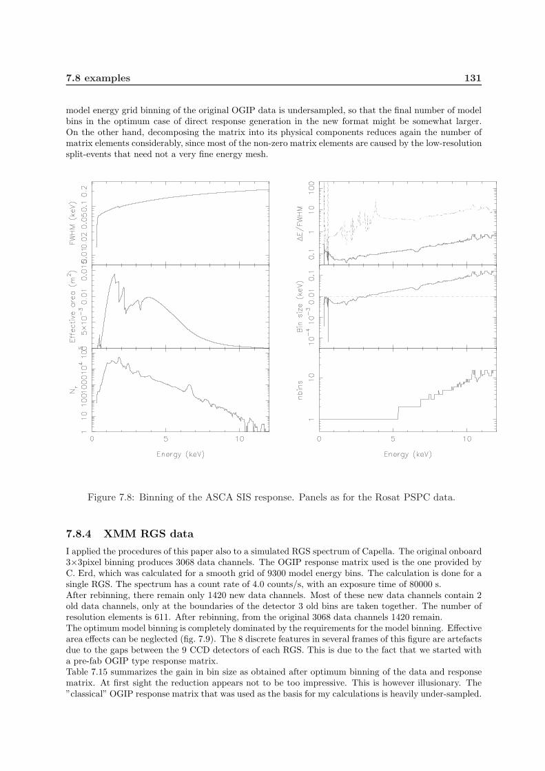
7.8 examples 131
model energy grid binning of the original OGIP data is undersampled, so that the final number of modelbins in the optimum case of direct response generation in the new format might be somewhat larger.On the other hand, decomposing the matrix into its physical components reduces again the number ofmatrix elements considerably, since most of the non-zero matrix elements are caused by the low-resolutionsplit-events that need not a very fine energy mesh.
Figure 7.8: Binning of the ASCA SIS response. Panels as for the Rosat PSPC data.
7.8.4 XMM RGS data
I applied the procedures of this paper also to a simulated RGS spectrum of Capella. The original onboard3×3pixel binning produces 3068 data channels. The OGIP response matrix used is the one provided byC. Erd, which was calculated for a smooth grid of 9300 model energy bins. The calculation is done for asingle RGS. The spectrum has a count rate of 4.0 counts/s, with an exposure time of 80000 s.After rebinning, there remain only 1420 new data channels. Most of these new data channels contain 2old data channels, only at the boundaries of the detector 3 old bins are taken together. The number ofresolution elements is 611. After rebinning, from the original 3068 data channels 1420 remain.The optimum model binning is completely dominated by the requirements for the model binning. Effectivearea effects can be neglected (fig. 7.9). The 8 discrete features in several frames of this figure are artefactsdue to the gaps between the 9 CCD detectors of each RGS. This is due to the fact that we started witha pre-fab OGIP type response matrix.Table 7.15 summarizes the gain in bin size as obtained after optimum binning of the data and responsematrix. At first sight the reduction appears not to be too impressive. This is however illusionary. The”classical” OGIP response matrix that was used as the basis for my calculations is heavily under-sampled.

132 Response matrices
Table 7.15: Rebinning of XMM RGS data
Parameter original final reductionOGIP value factor (%)
Data channels 3068 1420 46.3Model bins 9300 5964 64.1Matrix elements 2525647 783631 31.0
Would it have been sampled properly, then the model energy grid should have a size of a few hundredthousand bins! Since this causes the response matrix to be massive and disk consuming, the undersampledmatrix was created; this matrix can be safely used for spectral simulations, but is insufficient for flightdata analysis. It is exactly for that reason that the curren theoretical framework has been set up!
Figure 7.9: Binning of the XMM RGS response. Panels as for the Rosat PSPC data.
7.9 References
Arnaud, K.A., 1996, Astronomical Data Analysis Software and Systems V, eds. Jacoby G. and BarnesJ., p17, ASP Conf. Series volume 101.
Eisenhart, C., 1938, Bull. Am. Math. Soc. 44, 32.Jerri, A.J., 1977, Proc. of the IEEE 65, 1565.

7.9 References 133
Kaastra, J.S., Mewe, R., Nieuwenhuijzen, H., 1996, UV and X-ray spectroscopy of astrophysical andlaboratory plasmas, eds. K. Yamashita and T. Watanabe, p. 411, Univ. Acad. Press.
Shannon, C.E., 1949, Proc. IRE 37, 10.Weiss, P., 1963, Am. Math. Soc. Notices 10, 351

134 Response matrices

Chapter 8
Installation and testing
8.1 Testing the software
After installing the software, SPEX can be tested quickly as follows.Goto the directory $(SPEX)/test. Type the following in the terminal window:
spex
log exe test
quit
The above should produce a plot mytest.cps, which should be identical to the file test.cps in the samedirectory (except for the date string).Also, at the end of your output on the terminal you should have the following (except for machine-dependent rounding errors):
Chi-squared value : 1009.59
Degrees of freedom: 266
parameter Chi**2 Delta Delta
value value parameter Chi**2
----------------------------------------------------
5.66249 1010.50 -6.613350E-02 0.91
5.59636 1013.28 -0.132267 3.69
5.65690 1010.66 -7.172966E-02 1.07
5.63537 1011.41 -9.326029E-02 1.81
5.63051 1011.60 -9.811878E-02 2.01
5.63117 1011.58 -9.745693E-02 1.98
5.79476 1010.45 6.613350E-02 0.85
5.86089 1012.87 0.132267 3.27
5.80945 1010.87 8.082247E-02 1.27
5.82815 1011.43 9.951925E-02 1.83
5.83308 1011.62 0.104452 2.03
5.83240 1011.59 0.103778 2.00
Parameter: 5.7286 Errors: -9.74569E-02, 0.10378
Normal end of SPEX
You made 1 errors.
Thank you for using SPEX
STOP
The above test run is a simple single temperature fit to the MOS1 spectrum of an annulus in the clusterof galaxies A 1795.

136 Installation and testing

Chapter 9
Acknowledgements
9.1 Acknowledgements
We would like to express our special thanks to numerous people who have substantially contributed tothe development of various aspects of this work, in alphabetical order:Frans Alkemade, Gert-Jan Bartelds, Ehud Behar, Alex Blustin, Irma Eggenkamp, Andrzej Fludra, EdGronenschild, Theo Gunsing, Jorgen Hansen, Wouter Hartmann, Kurt van der Heyden. Fred Jansen,Jelle Kaastra, Jim Lemen, Duane Liedahl, Pasquale Mazzotta, Rolf Mewe, Hans Nieuwenhuijzen, Bertvan den Oord, Ton Raassen, Hans Schrijver, Karel Schrijver, Janusz Sylwester, Rob Smeets, KatrienSteenbrugge, Jeroen Stil, Dima Verner, Jacco Vink, Frank van der Wolf.During the years the many people have contributed as follows:Most software is written by Kaastra. Nieuwenhuijzen contributed to the software design.The line and continuum emission routines were written by Kaastra, based on previous routines by Mewe,Gronenschild, van den Oord, and Lemen (1981-1986).The line and continuum emission data are based on the work by Mewe and Kaastra. The photo-ionizationcross-sections have been provided by Verner. Liedahl contributed to the Fe-L calculations. Nieuwenhui-jzen, Raassen and Hansen contributed to the extension of the atomic database.Behar and Raassen contributed to the atomic data for the absorption models.Mazzotta worked on the ionization balance.The non-equilibrium ionization balance routine was developed by Jansen, based on earlier work by HansSchrijver (1974) and Gronenschild (1981).The SNR models are based on the work by Kaastra and Jansen (1992), with further extensions andtesting by Stil, Eggenkamp and Vink.Lemen, Smeets, and Alkemade developed an earlier version (1986-1990) of a spectrum synthesis program.The philosophy of the fitting procedure is based on the experiences obtained with the fitting of EXOSATdata, especially on the software package ERRFIT designed by Jansen and Kaastra.The original DEM modelling was based on the work by Sylwester and Fludra (1980), while the currentDEM regularisation algorithm has been designed by Karel Schrijver and Alkemade. Bartelds contributedto the testing of these models.The first version (1.0) of the documentation has been prepared – with starting help by Gunsing – byvan der Wolf and Nieuwenhuijzen. The second version was set-up by Kaastra with contributions fromSteenbrugge, van der Heyden and Blustin.

138 Acknowledgements

Bibliography
[1973] Allen, C.W., 1973, Astrophysical quantities, 3rd Ed., Athlone Press, London
[1989] Anders, E., & Grevesse, N., 1989, Geochimica et Cosmochimica Acta 53, 197
[1985] Arnaud, M., & Rothenflug, R., 1985, A&A Supp 60, 425
[1992] Arnaud, M., & Raymond, J.C., 1992, ApJ 398, 394
[2004] Bautista, M.A., Mendoza, C., Kallman, T.R., & Palmeri, P., 2004, A&A 418, 1171
[2002] Behar, E., & Netzer, H., 2002, ApJ 570, 165
[2002] Behar, E., Sako, M., & Kahn, S.M., 2002, ApJ 563, 497
[1994] Caldwell, C.D., Schaphorst, S.J., Krause, M.O., & Jimenez-Mier, J., 1994, J. Electron. Spectrosc.Relat. Phenom., 67, 243
[2003] Draine, B.T., 2003, ApJ, 598, 1026
[2005] Garcıa, J., Mendoza, C., Bautista, M.A., et al., 2005, ApJS, 158, 68
[2000] Gorczyca, T.W., 2000, Phys. Rev. A, 61, 024702
[1992] Grevesse, N., Noels, A., Sauval, A.J., 1992, in: Coronal Streamers, Coronal Loops and Coronaland Solar Wind Composition, Proc. 1st SOHO Workshop, ESA SP-348, ESA Publ. Div., ESTEC,Noordwijk, p. 305
[1998] Grevesse, N., & Sauval, A.J., 1998, ScScRev 85, 161
[2005] Gu, M.F., Schmidt, M., Beiersdorfer, P, et al., 2005, ApJ, 627, 1066
[2004] Juett, A.M., Schulz, N., & Chakrabarty, D., 2004, ApJ, 612, 308
[1989] Kaastra, J.S., & Barr, P., 1989, A&A 226, 59
[1993] Kaastra, J.S., & Jansen, F.A., 1993, A&A Supp 97, 873
[2004] Kaastra, J.S., Tamura, T., Peterson, J.R., et al., 2004, A&A 413, 415
[1994] Krause, M.O., 1994, Nucl. Instrum. Methods Phys. Res., 87, 178
[1991] Laor, A., 1991, ApJ 376, 90
[2003] Lodders, K., 2003, ApJ, 591, 1220
[1995] Magdziarz, P., Zdziarski, A.A., 1995, MNRAS 273, 837
[2004] Mendoza, C., Kallman, T.R., Bautista, M.A., & Palmeri, P., 2004, A&A 414, 377
[1983] Morrison, R., McCammon, D., 1983, ApJ 270, 119
[2001] Nahar, S.N., Pradhan, A.K., & Zhang, H.L., 2001, Phys. Rev. A. 63, 060701
[2002] Olalla, E., Wlison, N.J., bell, K.L., Martin, I., & Hibbert, A., 2002, MNRAS, 332, 1005
[2003] Palmeri, P., Mendoza, C., Kallman, T.R., Bautista, M.A., & Melendez, M., 2003, A&A 410, 359

140 BIBLIOGRAPHY
[2003] Peterson, J.R., Kahn, S.M., Paerels, F.B.S., et al. 2003, ApJ 590, 207
[1999] Phillips, K.J.H., Mewe, R., Harra-Murnion, L.K., et al., 1999, A&A Supp. 138, 381
[2004] Porquet, D., Kaastra, J.S., Page, K.L., et al., 2004, A&A 413, 913
[2003] Pradhan, A.K., Chen, G.X., Delahaye, F., Nahar, S.N., & Oelgoetz, J., 2003, MNRAS, 341, 1268
[1976] Ross, J.E., & Aller, L.H., 1976, Science 191, 1223
[1994] Rumph, T., Bowyer, S., & Vennes, S., 1994, AJ 107, 2108
[1979] Rybicki, G.B., & Lightman, A.P., 1979, Radiative processes in astrophysics, Wiley, New York
[2005] Steenbrugge, K.C., Kaastra, J.S., Crenshaw, D.M., et al., 2005, A&A 434, 569
[1985] Sunyaev, R.A., & Titarchuk, L.G., 1985, A&A, 143, 374
[1994] Titarchuk, L., 1994, ApJ, 434, 570
[1995] Hua, X.M., & Titarchuk, L., 1995, ApJ, 449, 188
[1995] Verner, D.A., & Yakovlev, D.G., 1995, A&AS 109, 125
[1996] Verner, D.A., Verner, E.M., & Ferland, G.J., 1996, At. Data Nucl. Data Tables 64, 1
[1995] Wheaton, W.A., Dunklee, A.L., Jacobson, A.S., et al., 1995, ApJ 438, 322
[1994] Zycki, P.T., Czerny, B., 1994, MNRAS 266, 653
[1999] Zycki, P.T., Done, C., Smith, D.A., 1999, MNRAS 305, 231

Index
abundance, 11ASCA, 7ascdump, 13
BeppoSAX, 7bin, 15
calculate, 15clusters of galaxies, 8command files, 28comp, 16
data, 17dem, 18distance, 20distance units, 20Doppler broadening, 44
egrid, 22elim, 23error, 24
file formats, 123fit, 25flux, 20free-bound emission, 44
ibal, 26ignore, 27ion, 27
log, 28
mekal, 45menu, 29multiply, 30
obin, 31
par, 31plot, 34plot, axis scales, 90plot, axis units, 90plot, captions, 88plot, colours, 82plot, devices, 81plot, line types, 84
plot, symbols, 89plot, text, 85plot, types, 81
quit, 38
Respons matrix, 99
sector, 38shiftplot, 39show model, 30simulate, 40sky sector, 20step, 41supernova remnants, 8syserr, 42system, 43
use, 43
vbin, 45
watch, 46
XMM-Newton, 7