kalman filtering estimation of unobserved rational...
TRANSCRIPT
Journal of Econometrics 20 (1982) 255-284. North-Holland Publishing Company
KALMAN FILTERING ESTIMATION OF UNOBSERVED RATIONAL EXPECTATIONS WITH AN APPLICATION TO THE GERMAN
HYPERINFLATION*
Edwin BURMEISTER
University of Illinois, Champaign, IL 61820, USA
University of Virginia, Charlottesville, VA 22901, USA
Kent D. WALL
Unioersity of Virginia, Charlottesville, VA 22901, USA
Received September 1980, final version received April 1982
The assumption that rational expectations always lie on a convergent path is subject to an empirical test using the German hyperinflation data. The estimation technique employs a Kalman filtering algorithm. After presenting a brief background for the convergent expectations problem and a derivation of the various model specifications, a generalized expectations model and its attendant Kalman filtering estimation technique are discussed. Additional estimation details and empirical results a;e then presented. Based on an assumption of normally distributed errors, the null hypothesis of convergent paths is rejected in all situations involving a deterministic specification of the evolution of the unobserved parameter which characterizes the convergent path. The same null hypothesis is rejected in four of the six cases corresponding to a stochastic specification of the evolution of the unobserved parameter which characterizes the convergent path. A discussion of these findings, their economic significance, and suggestions for further research concludes the paper.
1. Introduction
Elsewhere Burmeister (1980, 1982) has summarized the conceptual problems which arise in rational expectations modelling due to the common assumption that rationally formed expectations always lie on convergent paths. When this assumption is not made - and sometimes even when it is - the model is not determinant in the sense that there exist many stochastic paths for the actual variables, all of which are consistent both with equilibrium in every time period and with the rational expectations
hypothesis. Accordingly, since the postulate of convergent expectations
*The authors thank the National Science Foundation (SOC-76-03608-l) and the Federal Trade Commission (L0638) for financial support. Earlier comments from Robert P. Flood, Peter M. Garber, Bennett T. McCallum, and especially Kenneth J. Singleton ar.e gratefully acknowledged, and suggestions from two referees on an earlier version have provided many improvements. E. Burmeister is also grateful for research support from Duke University where some of this work was completed.
0304-4076/82/0000-0000/$02.75 0 1982 North-Holland
256 E. Burmeister and K.D. Wall, Estimation of rational expectations
carries with it important economic implications, and because the postulate is testable, a careful empirical investigation is merited.
A general framework within which this stability issue can be analyzed empirically has been developed by Wall (1980). A brief background for the convergent expectations question is provided in section 2, along with a derivation of the various model specifications we shall investigate. In section 3 we turn to the generalized expectation model and discuss how it is applied to obtain econometric estimates for data from the German hyperinflation. Additional details regarding estimation are presented in section 4 along with the empirical results.
2. A brief background and derivation of the basic model
The common assumption that rationally formed expectations always converge is crucial for at least three reasons. First, in many models this assumption is needed to determine a unique monetary equilibrium at each instant; without this convergence assumption, the future path of the economy modeled might be indeterminate, even without uncertainty. Second, the assumption of convergent expectations is commonly used to provide cross- equation restrictions which facilitate identification and econometric estimation; thus, most econometric estimates of rational expectations models are conditional upon this assumption. Third, if markets are not always in equilibrium, then there exist many cases in which the assumption of convergent expectations is untenable because it implies a contradiction.“’
‘See Burmeister, Flood and Turnovsky (1979). Burmeister (1980, 1982) provides a survey of some conceptual issues in rational expectations modelling, including the question of convergent expectations. Burmeister, Flood and Garber (1983) have shown that there is only one type of indeterminacy in rational expectation models; in the model considered here, there is indeterminacy whenever expectations are not convergent because there exist an infinity of equilibrium rational expectations paths with divergent expectations.
‘The fundamental problem of non-convergent price expectations which in turn may cause the problem of divergent actual prices, has been recognized for over twenty years. Writing in 1957, Samuelson discussed the issue of non-convergent paths:
So much for the avoidable difficulties introduced by infinite time. Now to return to the intrinsic difficulty. I shall call it the ‘tulip-mania phenomenon.’ Let the market maximize over any finite time, adding in at the end into the thing to be maximized a value for the terminal amount of grain left. At what level should this terminal grain be valued? We could extend the period in order to find out how much it is really worth in the remaining time left; but this obviously leads us back into our infinite regression, since there is always time left beyond any extended time. We are back into maximizing over infinite time.
But suppose we do what the market itself does in evaluating any stock Q(t) at any given date; suppose we simply evaluate it at the then ruling market price P,(t). Then we immediately run into the paradox that any speculative bidding up of prices at a rate equal to carrying costs can last foreoer. This is precisely what happens in a tulip mania or new- era bull stock market. The market literally lives on its own dreams, and each individual at every moment of time is perfectly rational to be doing what he is doing. [Samuelson (1957, pp. 215p216)].

E. Burmeister and K.D. Wall, Estimation of rationul expectations 251
In order to make the above ideas concrete, we shall base our discussion on the following simple stochastic monetary model:
md(t)-p(t)=b-a[p*(t+l,t)--*(t,t)], a > 0, (2.1 a)
p*(t + 1, t)= E,p(t + l), (2.lb)
m(t)=a,+cr,m(t- l)+s(t), (2.1 c)
(2.1 d)
where
PM =logarithm of the price level at time t;
E&t + h) =conditional expectation of p(t+h), h=O, 1,. ., formed at time t based upon all the information available at time t, which is assumed to be l(t)= {a, b, a,, cc,; p(t - l),p(t-2), . .; m(t- l),
m(t-2),...j;
m(t) =logarithm of the nominal stock of money at time t;
m*(t) =logarithm of the demand for the nominal stock of money at time
C
s(t) = serially uncorrelated stochastic disturbance in the money supply over the period (t - 1, t) with E[s(t) ( I(t)] = 0;
At) = serially uncorrelated stochastic disturbance in the price adjustment equation over the period (t - 1, t) with E[p(t) 1 I(t)] = 0;
a =a positive constant related to elasticity of the demand for real balances with respect to the expected rate of inflation;
b =a constant reflecting other variables influencing the demand for money which are held constant;
% @I =parameters of the money supply equation.
The system described by these four equations can be viewed as a simple extension of the modeis used by Sargent and Wallace (1973) and Black (1974) which now include stochastic disturbances in the money supply. Eq. (2.la) follows these previous authors in specifying the demand for real money balances to be a function of the anticipated rate of inflation over the period (t, t+ 1). These expectations are formed rationally in the sense of Muth (1961), and accordingly the expected price level is specified to equal the conditional expectations of actual prices, as described by (2.lb). Eq. (2.1~) determines the evolution of the stochastic money supply. Finally, eq. (2.ld) describes stochastic equilibrium in the money market. The stochastic
258 E. Burmeister and K.D. Wall, Estimation of rational expectations
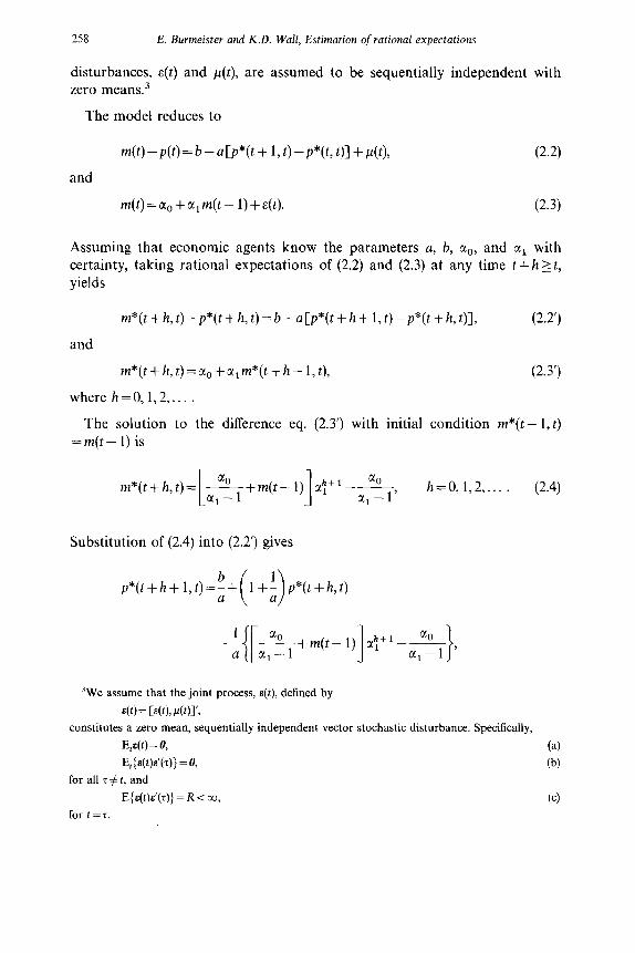
disturbances, c(t) and p(t), are assumed to be sequentially independent with zero means.3
The model reduces to
and
4) -PM = b - aCP*(t + 1, t) -P*k a + &),
m(t) = cI() + CC1 m(t - 1) + E(t).
(2.2)
(2.3)
Assuming that economic agents know the parameters a, b, cq,, and CI~ with certainty, taking rational expectations of (2.2) and (2.3) at any time t +hz t, yields
and
m*(t+h, t)-p*(t+h, t)=b-a[p*(t+h+ 1, t)-p*(t+h, t)], (2.2’)
m*(t+h,t)=ao+a,m*(t+h-l,t),
where h=O, 1,2 ,... .
(2.3’)
The solution to the difference eq. (2.3’) with initial condition m*(t - 1, r) = m(t - 1) is
+m(t-1) a;+l---, 3
@O
c!1- 1 h=0,1,2 ,... . (2.4)
Substitution of (2.4) into (2.2’) gives
p*(t+h+l,f)=$+ 1,; p*(t+h,t) ( )
1 -_ a i[
&++l+:+l-~}.
3We assume that the joint process, E(t), defined by
s(t) = [s(t), P(t)]‘>
constitutes a zero mean, sequentially independent vector stochastic disturbance. Specifically,
&s(t) = 0, (4 E,{E(t)E’(T)} =6 (b)
for all T # t, and
E{E(t)&‘(T)} = R < co, (4 for t=5.

E. Burmeister and K.D. Wall, Estimation of rational expectations 259
or
p*(t+h+ 1, t)= bee, -b-t@,
a(cQ- 1)
1 -;
[ &+m(t-1) cC:+r, h=0,1,2 )... .
1 I (2.5)
Since (1 + l/a)> 1 as the parameter a is positive, the only possibility for convergent price expectations arises from the ‘forward-looking’ solution to
(2.5),
p*(t + h, t) = -a,+b-bcr,
a, - 1
+(I +W” m(t_l)+ (2.6) U
Accordingly, the initial condition consistent with convergent expectations is
uniquely given by setting h =0 in (2.6); assuming that - 1 <(a,/(1 + l/a)) < + 1, this yields the special initial condition
P*(t, t) = -cl,+b-bet,
+ Ml
a,-1 1 +a-ucr, m(t-I)+* .
1 1 (2.7)
The crucial economic significance of (2.7) - which itself was derived by imposing the assumption that price expectations are convergent - stems
from the fact that it determines actual prices which are then given by
P(t) = P*k t) -cl(t) + 4th (2.8)
where p*(t, t) is determined from (2.7). To derive (2.8), subtract (2.2’) with h=O from (2.2) and subtract (2.3’) with h=O from (2.3), giving
and
Cm(t) -&)I - Cm*@, 4 -p*@, 91 = At),
m(t) - m*(t, t) = E(t).
Substituting the latter into the former yields (2.8).
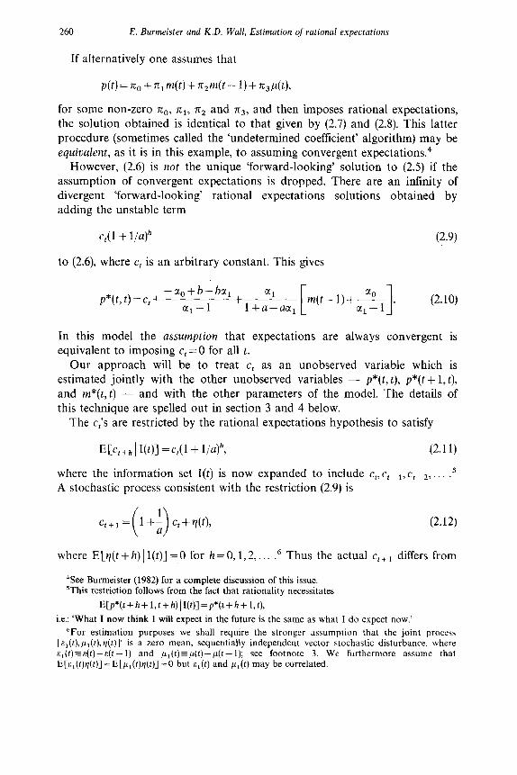
260 E. Burmeister and K.D. Wall, Estimation of rational expecrations
If alternatively one assumes that
p(t)=710+711m(t)+71,m(t- 1)+7L&),
for some non-zero no, rcl, IQ. and x3, and then imposes rational expectations, the solution obtained is identical to that given by (2.7) and (2.8). This latter procedure (sometimes called the ‘undetermined coefficient’ algorithm) may be equioalent, as it is in this example, to assuming convergent expectations4
However, (2.6) is not the unique ‘forward-looking’ solution to (2.5) if the assumption of convergent expectations is dropped. There are an infinity of divergent ‘forward-looking’ rational expectations solutions obtained by adding the unstable term
c,( 1 + l/a)” (2.9)
to (2.6), where c, is an arbitrary constant. This gives
p*p, t) = c, + -&)+b-bCX,
cr,-1 +
u1
1 +a--a@, [ rn(l-l)+S
I (2.10)
1
In this model the assumption that expectations are always convergent is equivalent to imposing c, = 0 for all t.
Our approach will be to treat c, as an unobserved variable which is estimated jointly with the other unobserved variables - p*(t, t), ~*(t+ 1, t), and m*(t, t) - and with the other parameters of the model. The details of this technique are spelled out in section 3 and 4 below.
The c,)s are restricted by the rational expectations hypothesis to satisfy
ECct., (WI =ct(l + l/4”, (2.11)
where the information set I(t) is now expanded to include ct, c,_ 1, c,_ 2,. . .5 A stochastic process consistent with the restriction (2.9) is
(2.12)
where E[q(t + h) 1 I(t)] = 0 for h = 0, 1,2,. . . .6 Thus the actual ct+ 1 differs from
‘See Burmeister (1982) for a complete discussion of this issue. ‘This restriction follows from the fact that rationality necessitates
ECp*(t+h+l,t+h)lI(t)]=p*(t+h+l,t),
i.e.: ‘What I now think I will expect in the future is the same as what I do expect now.’
‘For estimation purposes we shall require the stronger assumption that the joint proce\\ [cI(t),pl(t), q(t)]’ is a zero mean, sequentially independent vector stochastic disturbance, where &,(t)=&(t)--E(t-1) and pI(t)=p(t)-p(t-1); see footnote 3. We furthermore assume that E[z,(t)s(t)]=E[flI(t)~(t)]=O but cl(t) and p,(t) may be correlated.

E. Burmeister and K.D. Wall, Estimation of rational expectations 261
the expectation E[c,+~ /I(t)] by th e random error term y(t) which we assume
has finite variance. Our complete model consists of eqs. (2.3), (2.8) and (2.12).
Derivation in difference form
Estimation difficulties were encountered which were circumvented by respecifying the model in first differences. Thus we define the inflation rate
expected
7c*(t+h,t+h)-_P*(t+h+l,t+h)-p*(t+h,1+h),
and the corresponding actual inflation rate
7L(t+h)-p(t+h+ 1)-p(t+h), h=O,1,2 )... .
Likewise, the expected and actual money growth rates are defined as
g*(t+h,t+h)-m*(t+h+l,t+h)-m*(t+h,t+h),
and
(2.13)
(2.14)
(2.15)
g(t+h)-m(t+h+l)-m(t+h), h=O, 1,2 ,...,
respectively. Moreover, for all h = 0, 1,2,. . we have that
(2.16)
and
E[n*(t + h, t + h) ) I(t)] = Ir*(t + h, t), (2.17)
E[g*(t + h, t + h) 1 I(t)] =g*(t+ h, t). (2.18)
From eq. (2.2),
g(t+h)-7t(t+h)=-a[n*(t+h+l,t+h+l)-n*(t+h,t+h)]
+p(t+h+ l)-p(t+h),
for all h = 0, 1,2,. . ., while (2.3) implies that
(2.19)
g(t+h)=a,g(t+h-l)+E(t+h+l)-E(t+h), h=O,1,2 ,... . (2.20)
262 E. Burmeister and K.D. Wall, Estimation of rational expectations
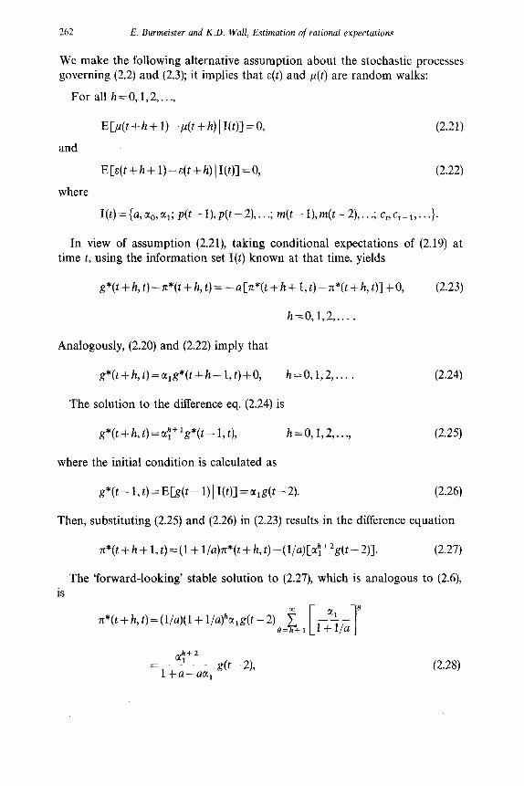
We make the following alternative assumption about the stochastic processes governing (2.2) and (2.3); it implies that s(t) and ,u(t) are random walks:
For all h=O, 1,2 ,...,
E[&+h+l)-&+h))I(t)]=O, (2.21)
and
E[.s(t+h+ 1)-e(t+h) 1 I(t)] =O, (2.22)
where
I(t)={a&+X,; I$- l), p(t-2),. . .; m(t- l),m(t-2),. . .; CtrC,_l,. . .>.
In view of assumption (2.21), taking conditional expectations of (2.19) at time t, using the information set I(t) known at that time, yields
g*(t + h, t) - n*(t + h, t) = - a[n*(t + h + 1, t) - 7c*(t + h, t)] + 0, (2.23)
h=0,1,2 )...
Analogously, (2.20) and (2.22) imply that
g*(t+h,t)=cl,g*(t+h-l,t)+O, h=0,1,2 )... . (2.24)
The solution to the difference eq. (2.24) is
g*(t + h, t) = a;+ ‘g*(t - 1, t), h=0,1,2 ,..., (2.25)
where the initial condition is calculated as
g*(t-l,t)=ECg(t-l))I(t)]=cl,g(t-2). (2.26)
Then, substituting (2.25) and (2.26) in (2.23) results in the difference equation
(2.27)
The ‘forward-looking’ stable solution to (2.27), which is analogous to (2.6), is
n*(t+h,t)=(l!a)(l+l/a)“alg(t-2)e=~+1 & ’ [ 1
h+2
= 1 +:_,,, &-32 (2.28)

E. Burmeister and K.D. Wail, Estimation of rational expectations 263
provided - 1~ la,/(l + l/a)\ < + 1 as we shall assume. Thus setting h=O and
h= 1 in (2.28) we may calculate
and
7c*p, t) = x:
1 +a--act, go - 212 (2.29)
n*(t+l,t)=l+;Taz g(t - 2). 1
(2.30)
It is easily verified that (2.29) and (2.30) satisfy (2.27) with h=O; they represent rationally formed expected inflation rates which are consistent with the assumption of convergent expectations.
In general, however, the solutions to (2.27) which are consistent with ‘forward-looking’ rational expectations are of the form
hi2
?r*(r+h,t)=c,(l+lia)h+l+~_ua g(t-21, h=O,1,2 )...) (2.3 1) 1
where the c,‘s satisfy (2.12). Note that (2.31) and (2.28) are equivalent if and only if c,=O in (2.31). However, for non-zero c,, (2.31) is not convergent since
lim,, p) (1+ l/a)“= + co. In view of (2.12), we see that
7cn*(t, t) = c, + 4
1 +a-ucc, g(t - 2), (2.32)
and
7-c*(t+1,t+1)=Ct+l+ @:
1 +a--a@, & - 1). (2.33)
Substituting (2.32) and (2.33) into (2.19) with h=O gives
g(w)=-u(c,+I-c,)-I+~~u~I k(t-1)-g(t-2)]
+ cl@ + 1) - PL(G (2.34)
We now take conditional expectations of (2.34), using the fact that E[c,+ 1 (I(t)] =c,(l + l/u) from assumption (2.12),
g*(t, t)-7c*(t, t)= -c,- UC!:
1 +a-ua, M--l)-_g(t-m (2.35)

264 E. Burmeister and K.D. Wall, Estimation of rational expectations
Subtracting (2.34) from (2.35) yields
n(t)-n*(t)= ac,, 1 -Cl +a)c,+E(t+ l)-I--(t+ l)+p(t), (2.36)
since g(t)-g*(t, t)=~(t+ l)-&(t). The first two terms on the right-hand side of (2.36) sum to aq(t), and therefore
E[n(t)-z*(t, t) (I(t)] =O,
confirming that expectations have been formed rationally. As noted below, we found it necessary to consider a second-order money
growth rate process. Thus following Flood and Garber (1980), we also have estimated another version of the model for which the model supply process is respecified as
g(t)=cc,+(l +~~)g(t-l)--a,g(t-2)+o(t), (2.37)
where w(t) is a white noise process. Eq. (2.37) implies
g*(t+~,~)=g(l-2)+~(l-a:+~)Cg(t2)-g(t-3)1 1
+*(h+2)+*(u:-“-l). 1
(2.38)
These expectations for the rate of growth of the money supply then yield the following specification for the evolution of the inflation expectations:’
at - l- +1-Cc, (
N: 1 +a-act, 1
‘Eq. (2.39) is derived from
x rg(t-l)-2g(t-2)+g(t-3)]. (2.39)
x*(t+h;t)c,(l+l/a)h+(l/a)(l+l/a)h f (1+1/a)-‘g*(t+O-1,t) o=h+ 1
=~,(l+l/a)~+g(t-2)+2 (h+2+a) 1 %a1 +------_- i IIt, MI h-i1
(l-a,)2 1+a--act, l-a,_ 1 [ a1 l-U, 1 +a-act,
1 IMt-2)-&d-3)1, 1 which is the general solution to the difference equation
n*(t+h+l,t)=(l+l/a)rr*(t+h,t)-(l/a)g*(t+h,t),
i.e.. it is the solution to (2.23).

E. Burmeister and K.D. Wall, Estimation of rational expectations 265
Finally, the actual rate of inflation is given by
71(t) = z*(t, t) + a@) + o(t) - p(t + 1) + p(t), (2.40)
with E[rc(t) ( I(t)] = rc*(t, t), again confirming rational expectations.
3. A state space model of expectation formation
The empirical investigation of the convergent expectations question can be approached in a number of ways. Perhaps the most attractive from a traditional econometric viewpoint is to solve the system analytically and substitute these solutions into the behavioural system (2.2)-(2.3). The result is a system of equations involving interequation restrictions that are amenable, at least in principle, to standard regression techniques. While such an approach eliminates the bothersome appearance of unobserved variables like ~*(t + h, t) and c,, it may not be the least complicated since it necessitates the formation of convolutions on m(t- 1) and p(t).
An alternative approach, and the one taken here, is to retain the explicit reference to the unobserved variables. To wit, a state space form representation is employed wherein the unobserved variables become state variables. Drawing upon a well-developed theory from control engineering, it is then possible to obtain simultaneously estimates of both the model parameters and the unobserved expectations. This permits a much easier test of certain hypotheses than would otherwise be the case. Since such an approach is relatively unfamiliar, we first present the state space interpretation of models introduced in section 2, and describe its estimation.
3.1. The state space model
Let x(t) be an n-vector of state variables, u(t) an m-vector of ‘inputs’, and y(t) an l-vector of ‘outputs’. Then a state space,model relating these variables to one another is given by
x(t + 1) = h(t) + Gu(t) + rq(t), (3.1)
y(t) = Hx(t) + h(t) + E(t). (3.4
Both q(t) and E(t) denote vectors of random variables such that
and
W(t)1 =O, E {E(t)} = 0,
E{&), V’(S))= QL E{+), 0)) =RL
266 E. Burmeister and K.D. Wall, Estimation of rational expectations
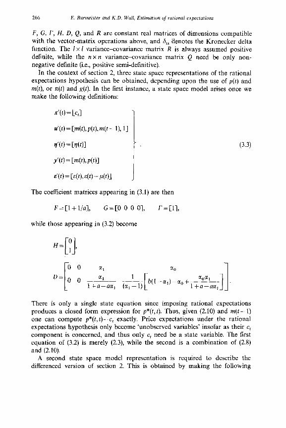
F, G, r, H, D, Q, and R are constant real matrices of dimensions compatible with the vector-matrix operations above, and 6,, denotes the Kronecker delta function. The 1 x 1 variance-covariance matrix R is always assumed positive definite, while the n x n variance-covariance matrix Q need be only non-
negative definite (i.e., positive semi-definitive). In the context of section 2, three state space representations of the rational
expectations hypothesis can be obtained, depending upon the use of p(t) and m(t), or z(t) and g(t). In the first instance, a state space model arises once we make the following definitions:
x’(t) = cc,1 1
u’(t) = Cm(t), p(t), m@ - 1),11
tl’(t) = CrWl
f(t) = Cm(t), p(t)1
w = [4t), g(t) - At)1 J The coefficient matrices appearing in (3.1) are then
F = [ 1 + l/a], G=[O 0 0 01, r=Cll,
while those appearing in (3.2) become
(3.3)
H=
00 a,
i
a0
D=o 0 1 +;:aa, 1
. (a1 _ 1) [ b(I-a+ao+ 1 +:“h,, 11 There is only a single state equation since imposing rational expectations produces a closed form expression for p*(t, t). Thus, given (2.10) and m(t - 1) one can compute p*(t, t)-c, exactly. Price expectations under the rational expectations hypothesis only become ‘unobserved variables’ insofar as their c, component is concerned, and thus only c, need be a state variable. The first equation of (3.2) is merely (2.3), while the second is a combination of (2.8) and (2.10).
A second state space model representation is required to describe the differenced version of section 2. This is obtained by making the following

E. Burmeister and K.D. Wall, Estimation of rational expectations
definitions once the IX,, term has been reintroduced in (2.20),
x’(t) = cc,, c, + 1 - 4
267
u’(t) = k(t), n(t), go - 11, go - 2),11 I
tl’@) = L-r@), r@ + 111 (3.4)
J+(t) = k(t), Ml
d(t) = [i?(t + 1) - E(t), s(t + 1) -s(t) - p(t + 1) + l*(t)] I
The coefficient matrices of the state equations for this version of the model
become
[
1+1/a 0
F= (l/a)(l+l/a) 0 ' G= 1 I : x : : kJ r=[lo ;I; while those of the output equation, (3.2) become
0 0
‘I I
00 a, 0 NO
H= 0 a'
D= (1 +ab, --cc2
O O l+a-acr, l+a-act, BO
1.
The first state equation is just (2.12). The second represents the evolution of c,+ 1 -c,, which can be obtained by noting that
C t+2-Cr+1- -(ll&+l+v(t+l)
=(l/a)(l+ l/a)c,+(l/a)vl(t)+rl(t+ 1).
The two equations in (3.2) are derived from (2.20) and (2.34), respectively. As described in the next section, it was found necessary to respecify a
second-order money growth rate process in place of (2.20). Following Flood and Garber (1980), g(t) was assumed to obey a first-order autoregression in its second differences, i.e.,
or
k(t) -s(t - 111 = @o + a, t-go - 1) -g(t - 211 + ~W,
g(t) = CIo + (1 + a1)g(t - 1) - @.,g(t - 2) + o(t).

268 E. Burmeister and K.D. Wall, Estimation of rational expectations
Here o(t), as usual, is assumed to be a zero mean white noise process. With g(t) obeying the above, a third state space model representation is obtained by employing the following definitions:
x’(t) = cc,, cr + 1 - 4
u’(r) = k(t), r+), g(r - l), g(r - 2), g(r - 3), 11
rl’(t) = C?(t)> Y@ - 1)l
Jw = cm WI
4t) = C40, w(t) - cl@ + 1) + P(t)1 1.
(3.5)
The coefficient matrices of the state space representation for this version of the model become
F=
while those of the output equation, (3.2), become
A= l+&_-_. [
4 1 I 1 l-a, l+a-acr, ’ B= l+S_-_.
[
201: 1 1 1 l-a, l+a--aa, ’ c= _?L-.
[ 4 1
l-a, 1 l-a, l+u-ua, . The state equations appear exactly as in the model associated with (3.4). The only differences appear in the output equations.
Conversion of the model into (3.1)-(3.2) is desirable primarily to permit the use of Kalman filtering. Estimates of the elements of x(t) can be directly obtained, and these estimates are minimum-mean-square error. Furthermore, the Kalman filter can be employed to produce innovations sequences (residuals) which may be used to iteratively compute estimates of the model

E. Burmeister and K.D. Wall, Estimation of rational expectations 269
parameters along with estimates of x(t). Moreover, both state and parameters estimation can be effected in the absence of stability and stationarity assumptions. This makes the state space representation and its attendant estimation via Kalman filtering particularly well suited to address the issues raised in section 1, and is the prime reason for representing the model in the form (3.1)-(3.2). In estimation algorithm is briefly described below.
3.2. State estimation
For expositional convenience first consider the problem of estimating x(t)
given the parameters of F, G, r, H, and D, together with the first two moments of y(t) and u(t). If i(t,z) denotes the minimum-mean-square error estimate of x(t) given the model and all observed data up through time z,
Y’= Mlbo)~~~ .&)},
U’= (u(l), u(2), . . ., u(z)},
then i(t, t) is produced by the following recursive computation:
i(t + 1, t) = F.f(t, t) + Gu(t), (34
P(t + 1, t) = FP(y, t)F’ + rQl-‘, (3.7)
B(t+ 1, t)=HP(t+ l,t)H’+ R, (3.8)
E^(t + 1, t) =y(t + 1) - Hf(t + 1, t) - Du(t + l), (3.9)
K(t+l)=P(t+l,t)H’B-‘(t+l,t), (3.10)
_?(t+l,t+l)=f(t+l,t)+K(t+l)E^(t+l,t), (3.11)
P(t+l,t+l)=[Z-K(t+l)H]P(t+l,t), (3.12)
for t, st_l7: P(t + 1, t) is the variance-covariance matrix of the estimation matrix error in i(t + 1, t), i.e.,
P(t+l,t)=E{[x(t+l)--(t+l,t)][x(t+l)--(t+l,t)]’).
B(t + 1, t) is the variance-covariance matrix of the innovation, i.e.,
B(t+l,t)=E{E^(t+l,t)E^(t+l,t)‘).

270 E. Burmeister and K.D. Wall, Estimation qf rational expectations
The initial values for a(t, t) and P(t, t) are assumed known and given by
i(t,, to) =a(O) = E{x(t,) g iven all information at time to},
P(b, k,) = P(O) = E{ C+J - WI Cx@o) - WI'}
Thus P(t,,) is the variance-covariance matrix of the error in estimating x(t) given all observations up through time (z 2 t). The vector c(t + 1, t) represents the innovations process and is analogous to the model residuals used in econometric estimation. Eqs. (3.6)-(3.12) constitute the Kalman filter.
More efficient estimates of the states can be obtained by utilizing all the sample information available; i.e., i(t, T). This is referred to as the smoothed estimate. It is derived from the filtered estimate, i(t, t), by means of a reverse ‘sweep’ over the data from T back to t + 1. Broadly speaking, computation is as follows: the recursive Kalman filter is employed in reverse time ‘beginning’ at time T using a diffuse ‘prior’ for i(T, T + l), i.e., P(T, T+ 1) = cc. For any time t in the closed interval [0, T], this reverse time filter produces an estimate, -i-(t, t + l), alang with its corresponding variance-covariance matrix,
P(t, t + 1). This represents our best estimate of x(t) using data only over the interval [t + 1, T]. Combining this with our forward time estimate, i(t, t), using only data over the interval [0, t], gives us the desired result, -i-(t, T). The method of combination follows from a classical result in probability and statistics; namely, the optimal combination of two independent estimates a(t, t) [with precision matrix P-‘(t, t)] and .iZ(t, tt 1) [with precision matrix Pml(t,t+l)] is
i(t, T)=P(t, T)[P-‘(t,r)f(t, t)+P-‘(t, t+ l)a(t, t+ l)],
with corresponding precision matrix
P-‘(t,T)=P-‘(t,t)+P-‘(t,t+l).
Details of the smoothing algorithm employed below are given in Cooley,
Rosenberg and Wall (1977). Thus, once filtered estimates are obtained, they can be revised by the smoothing algorithm to produce the most efficient estimates of ~(t).s
3.3. Parameter estimation
Using the Kalman filter to generate model residuals enables the formation of a loss function that can be used in parameter estimation. The parameters
‘It can be shown that P(t, t)zP(t, T) for t, s t 5 7: This should be intuitively clear since, by definition, a(t, T) uses more information than x(t, t). See Jazwinski (1970, ch. 7) or Bryson and Ho (1969, ch. 13).

E. Burmeister and K.D. W&l, Estimation of rational expectations 271
to be estimated may not only include the unknown elements of H, D, and R (the parameters of the behavioral equations). but more importantly those of F, G, r, and Q. The algorithms for estimation of the unknowns in this manner are called ‘prediction error’ methods and, like the Kalman filter, are
thoroughly treated in the control literature [see Caines (1976), Ljung (1979) and Ljung and Caines (1979)]. The algorithm employed in the present study is outlined by the following steps:
Step 1. Collect the unknown parameters into a vector 8 of dimension N x 1. Denote an initial guess at its true value by 0’ and insert this into the Kalman filter eqs. (3.6))(3.12). Set i=O.
Step 2. Using the Kalman filter eqs. (3.6)-(3.12) compute the model innovations sequence {f(t+ 1, t); tests T- 1$ where P(t+ 1, t)=E^(t + 1, t,Oi) is an implicit function of 8’.
Step 3. Form the loss function J(0”) where
J(@) =i ‘f’ [i(tf 1, t)‘n,‘, ,!c^(t + 1, t) + In (det /1,+ r,,)], t0
(3.13)
and A+ If is some positive definite weighting matrix.
Step 4. Compute an improved estimate of 8, denoted @+I, such that _I(@+ ‘) 5 J(@). Use
8 i + 1 = @_ piM - 1 aJ(r@)/ae,
where pi is a (scalar) step size parameter and n/lie1 is a positive definite
N x N matrix such that in the limit (as i+~) it tends to the inverse Hessian of J. (See discussion,after Step 5.)
Step 5. Check to see if )~~‘+‘-0’~~<fi, and/or 1/?J(8i”)/118(1~62. If so, stop; f?+’ is accepted as the ‘best’ estimate of 8. Otherwise, set 13’ to @+I, i= i+ 1, and return to Step 2. If it is assumed that c(t) is normally distributed for each
t, and 4+1~, is set equal to B(t + 1, t), then approximare maximum likelihood estimates are obtained; see Anderson and Moore (1979).
The iterative algorithm given above requires an initial estimate, 8’; a convergence criterion, ii, and/or 6,; and expressions for the components of the gradient vector &J(0)/%. The gradients may be computed numerically using simple finite first differences of J(0) or analytically using a straightforward application of differential calculus to (3.13). The method by

212 E. Burmeister and K.D. Wall, Estimation of rational expectations
which pi and Mi computed depends on the particular function minimization algorithm employed. A Davidson-Fletcher-Powell Variable Metric algorithm is used here since then ML1 1s computed automatically, with aJ(0)/86 being the only user supplied information. Upon convergence M; ’ is the inverse Hessian of J(e) (i.e., the information matrix) and yields valuable information concerning estimated parameter standard errors, correlations (covariances), and indentitiability. In particular, once the algorithm converges, a simple scaling of M;’ produces an estimate of the parameter variance-covariance matrix. Not only is this estimate useful in hypothesis tests on elements of 0, but also in examining identifiability. Since local identifiability and asymptotic
non-singularity of the Hessian matrix are equivalent, a nearly singular M;’ indicates identification problems. In practice, this is most easily tested by converting the parameter variance-covariance matrix to a correlation matrix and examining the off-diagonal elements. Interparameter correlations near unity, say kO.996, lead to a singular condition suggesting an over- parameterized specification and lack of complete identification. Moreover, a singular Hessian for J(B) results in non-convergence of the numerical
optimization algorithm so that lack of convergence and lack of identification are highly related. These facts are extremely helpful in deciphering the estimation results given in section 4.
4. Estimation details and results
The state space model associated with the definitions in (3.3), (3.4), and (3.5) each contain six unknown parameters: a, LX,,, c(~, a;, and the two distinct elements of the symmetric 2 x 2 matrix R, CT: and r$. In order to guarantee that the estimates of R always be positive definite during estimation, the lower triangular Cholesky factorization was used to define the unknowns related to R; namely, R was represented as
A likewise representation was employed for the Q matrix, i.e.,
for the
for the
Q = Cot,1 [a,1
levels model, while
Q=[;ya :J[z 2y]
differenced models.

E. Burmeister and K.D. Wall, Estimation of rational expectations 273
The initial state estimate, a(O), and its error variance-covariance matrix, P(O), constitute another live unknowns. These were not estimated but fixed at a specified value since, asymptotically they do not affect the results.’ Thus the tI vector is defined as
Upon convergence of the iterative algorithm for 8, the Kalman filter is called to produce ‘filtered’ estimates a(t, t) for x(t), i.e.,
il(t, t) = E{c, 1 Y’, U’),
for the levels models, and
i,(t, t) = E{q ( Y’, Ut>,
for the differences models. Finally, given 8 and a(t, t), the smoothing algorithm is called to produce i(t, T) which constitute our best estimates of the state variables given all the sample information. These are to be interpreted as our conditional expectation (conditioned on the observed data sample) of the variables employed by a representative economic agent in forming the rational expectations consistent with the given model.
4.1. Estimation results
Estimation of (3.1)-(3.2) was carried out using price data taken from Zahlen zur Geldentwertung in Deutschland 1914 his 1923, Reimar Hobbing, Berlin, 1925. Money supply figures were taken from table VII of Flood and Garber (1980). The same period for both price and money covered January 1919 through June 1923. Six different bubble phenomena were considered, all lasting until June 1923 but beginning in different months. Beginning dates for the bubbles were: January 1919, October 1919, July 1920, June 1921, June 1922, and January 1923. The third, fifth, and sixth bubbles correspond exactly with those treated by Flood and Garber (1980).
Initial attempts to lit the levels model, (3.3), failed. No convergence in the iterative procedure was obtained due to severe negative correlation between
‘Given a completely observable model, it can be shown that the filter is uniformly asymptotically stable with asymptotic solutions independent of the initial data; see Jazwinski (1970), Bucy and Joseph (1968), for example.

214 E. Burmeister and K.D. Wall, Estimation of rational expectations
CI,, and a, (estimated at -0.994 after approximately sixty iterations). This problem was also evident in the serial correlation properties of the residuals in the money supply equation. For these reasons the levels model was abandoned in favor of the differenced version (3.4).
Two versions of (3.4) were estimated. In the first CI~ was estimated along with the other model parameters, while in the second it was constrained to unity (reflecting the belief that the money growth rate was best modeled as a perfect second difference). In both cases the residuals for the money growth rate failed to satisfy tests for no serial correlation, significant serial correlation being present at lag one. Hence, this model was dismissed from further consideration and a slightly more elaborate money supply process
specified. Estimation of the more elaborate model, (3.5), produced none of the
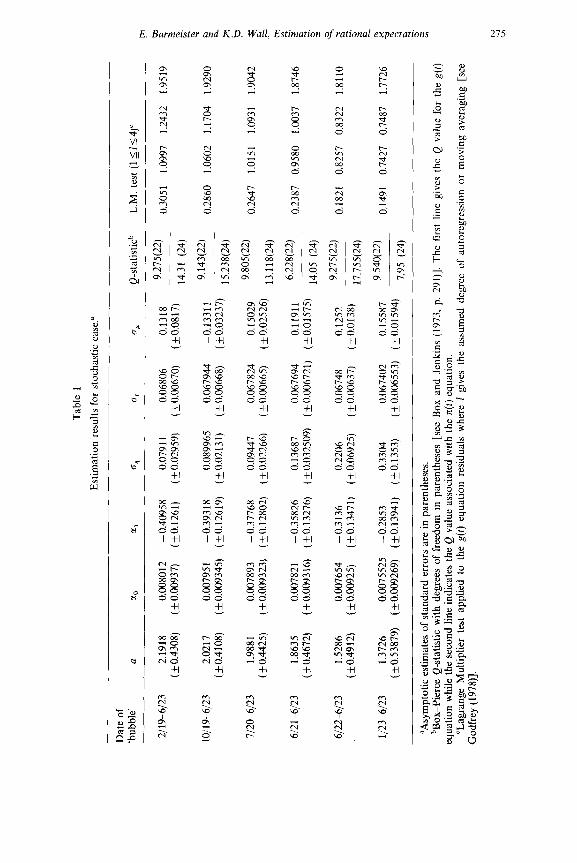
problems associated with the previous cases. Convergence of the iterative estimation scheme was achieved in each instance and all estimated residual series met the serial correlation tests. Results for this case are presented in tables 1, 2, and 310*‘1 and in fig. 1. The first table presents the parameters estimates. In each of the six bubbles a significant non-zero gs is obtained. Moreover, a slight negative correlation between a and CJ~ is revealed. The
second table presents the smoothed estimates for the c, trajectories and their associated estimation error variances. Significant c,‘s appear in the last two months of the sample for all bubbles except those bubbles starting in to June
1922 and January 1923. l2 This behavior is due to a combination of the
“All standard errors reported in table 1 require a special interpretation similar to that given in Flood and Garber (1980, fn. 18) because the state space representations associated with (3.3) and (3.4) are unstable (i.e., each has an F matrix with one eigenvalue equal to 1+ l/a which lies outside the unit circle), and result in a situation analogous to the ‘exploding regressor’ case in econometrics. Thus, we must view our data sample as one drawing from a cross-section of repeated hyperinflations, all with the same pre-1920 events and behavioral parameters. In this sense the length of the data sample is fixed at 40 observations (March 1920 through June 1923), while the number of repetitions, N, of this sample tends to infinity. The estimates obtained here then are both asymptotically consistent and normal [see Goodrich and Caines (1979)].
“The degrees of freedom for the g(t) equation Q statistic are obtained by interpreting this equation as a standard ARMA (2,0) model for g(t). For the n(t) equation the interpretation is not so clear since a state variable appears on the right-hand side; we no longer have an equivalent ARMA (p,q) model. What has been done is to assume the estimated residuals themselves comprise a given time series and that an ARMA (0,O) model has been lit. A Q- statistic test for ‘model’ adequacy t& translates into an approximate test for ‘whiteness’. Alternatively, both residuals could be subjected to a test of significance using as the 95% confidence band &2/,,& = +0.28 [see Box and Jenkins (1973, pp. 177, 178, 290)].
“The confidence regions are computed from the diagonal elements of the P(t, t) matrix in the filtered case, and P(t, T) matrix in the smoothed case. Each of these matrices implicitly depends on the 0 vector through the F, H, Q, and R matrices [see (3.6)-(3.12)]. Thus in computing these variances we are treating the parameters as known exactly, i.e., that the representative economic agent takes these parameter estimates as given. Incorporation of the uncertainty in 0 in generating both P(t,t) and P(t,T) requires solution of a nonlinear filtering problem for which only approximate solutions exist [see Jazwinski (1970, chs. 7 and S)].
Tab
le
1
Est
imat
ion
resu
lts
for
stoc
hast
ic
case
.a
Dat
e of
‘b
ubbl
e’
a cl
l Q
-sta
tistic
” L
.M.
test
(1
51<
4)”
2/19
-612
3 2.
1918
0.
0080
12
-0.4
0958
0.
0791
1 0.
0680
6 0.
1318
9.
275(
22)
0.30
51
1.09
97
1.24
32
1.95
19
(kO
.430
8)
(~0.
0093
7)
(+O
.t261
) (f
O.0
2959
) (+
_0.0
0670
) (k
O.0
817)
14
.31
(24)
10/1
9-61
23
2.02
17
0.00
7951
-0
.393
18
0.08
9965
0.
0679
44
-0.1
3311
9.
143(
22)
0.28
60
1.06
02
1.17
04
1.92
90
(+0.
4108
) (+
_0.0
0934
5)
(f_O
.126
19)
(+_0
.021
31)
(~0.
0066
8)
(kO
.032
37)
15,2
38(2
4)
7/2&
6/23
1.
988
1 0.
0078
93
- 0.
3776
8 0.
0944
7 0.
0678
24
0.15
029
9.80
5(22
) 0.
2647
1.
0151
1.
0931
1.
9042
(kO
.442
5)
(fO
.009
323)
(+
_0.1
2802
) (k
O.0
2266
) (k
O.0
0665
) (k
O.0
2526
) 13
,118
(24)
6/21
-612
3 1.
8635
0.
0078
21
-0.3
5826
0.
1368
7 0.
0676
94
0.11
911
6.22
8(22
) 0.
2387
0.
9580
1.
0037
1.
8746
(kO
.467
2)
(+_0
.009
316)
(k
O.1
3276
) (k
O.0
3250
9)
(kO
.006
721)
(k
O.0
1575
) 14
,05
(24)
6122
-612
3 1.
5286
0.
0076
54
-0.3
136
0.22
06
0.06
748
0.12
52
9.27
5(22
) 0.
1821
0.
8257
0.
8322
1.
8110
(kO
.491
2)
(&0.
0092
5)
(kO
.134
71)
(kO
.069
25)
(kO
.006
37)
(kO
.013
8)
17,7
55(2
4)
l/233
6/23
1.
3726
0.
0075
525
-0.2
853
0.33
04
0.06
7402
0.
1558
7 9.
540(
22)
0.14
91
0.74
27
0.74
87
1.77
26
(*0.
5387
9)
(+0.
0092
69)
(kO
.139
41)
(k0.
1353
) (f
0.00
6553
) (k
O.0
1594
) 7.
95
(24)
“Asy
mpt
otic
es
timat
es
of s
tand
ard
erro
rs
are
in p
aren
thes
es.
“Box
-Pie
rce
Q-s
tatis
tic
with
de
gree
s of
fr
eedo
m
in
pare
nthe
ses
[see
B
ox
and
Jenk
ins
(197
3,
p.
291)
].
The
fi
rst
line
give
s th
e Q
va
lue
for
the
g(t)
eq
uatio
n w
hile
th
e se
cond
lin
e in
dica
tes
the
Q v
alue
as
soci
ated
w
ith
the
rr(r
) eq
uatio
n ‘L
agra
nge
Mul
tiplie
r te
st
appl
ied
to
the
g(f)
eq
uatio
n re
sidu
als
whe
re
I gi
ves
the
assu
med
de
gree
of
au
tore
gres
sion
or
m
ovin
g av
erag
ing
[see
G
odfr
ey
(197
8)].

276 E. Burmeister and K.D. Wall, Estimation of rational expectations
Table 2
Smoothed estimates for c, and its error variance (stochastic case).
Date var (2,) C, var (2,)
- 0.96978E - 02 0.67962E -02
-O.l4638E-01 -0.35449E-02
0.62814E-02 O.l2753E-01 0.25363E-01 0.42444E-01
1919 0.65732E -01 0.74394E -01 0.65182E-01 0.60193E-01 0.62803E -01 0.71523E-01
0.60995E - 02 0.58531E-02 0.57661E-02 0.57353E-02 0.57244E - 02 0.57205E -02 0.57192E-02 0.57187E-02 0.57185E-02 0.57185E-02 0.57184E-02 0.57184E-02
0.51461E-01 O.l3465E-01
-O.l4556E-01 -0.20715E-01 -0.20090E-01 -O.l3201E-01
1920 -0.85290E-02 - 0.77643E - 02 -O.l0285E-01 -0.77554E-02 - 0.68827E - 02 - 0.49274E -02
0.57184E-02 0.57184E-02 0.57184E-02 0.57184E-02 0.57184E-02 0.57184E-02 OS7184E-02 0.57184E-02 0.57184E-02 0.57184E-02 0.57184E-02 0.57184E-02
-0.73732E -02 -0.59325E-02 -0.25324E-02
0.38328E-02 O.l3562E-01 0.25212E-02
1921 0.42244E -01 0,38616E-01 0.3941OE-01 0.39058E-01 0.22489E -01 0.25583E-01
0.57184E-02 0.57184E-02 0.571848-02 0.57184E-02 0.57184E-02 0.57184E-02 0.57184E-02 0.57184E-02 0.57184E-02 0.57184E-02 0.57184E-02 0.57184E-02
0.40303E - 02 0.55538E-01 0.40235E-01 0.29562E -01 0.48818E-01 0.68459E -01
1922 0.79930E-01 0.56356E-01 0.40878E-01 O.l3801E-01
-0.30168E-01 -O.l7545E-01
0.57184E-02 0.57184E-02 0.57184E-02 0.57185E-02 0.57185E-02 0.57187E-02 0.57191E-02 0.57202E - 02 0.57235E-02 0.57328E-02 0.57590E - 02 0.58332E-02
O.l9843E-01 0,51674E-02
1923 O.l1964E+OO 0.28851E+OO 0.468OOE + 00
0.60432E - 02 0.66370E - 02 0.83165E-02 O.l3065E-01 0.26503E-01
O.l8349E-01 0.28148E-01 0.38369E - 01
0.366OOE-01 0.84662E -01
-O.l2408E-01 -O.l6966E-01 -O.l653OE-01 -O.l1154E-01 -0.72770E-02 -0.65281E-02 -0.84264E-02 -0.64241E-02 -0.59086E-02 -0.44136E-02
-0.60923E-02 -0.48097E-02 -O.l9065E-02
0.31695E-02 O.l0986E-01 0.20197E -01 0.33643E-01 0.30889E-01 0.31698E-01 0.31950E-01 O.l8688E-01 0.20876E -01
0.33426E-01 0.43451E-01 0.32238E-01 0.24695E -01 0.36697E -01 0.55665E -01 0.65666E -01 0.48586E-01 0.38051E-01 O.l8189E-01
-O.l4239E-01 - 0.24994E - 02
0.29375E-01 0.25994E-01 0,12541E+00 0.27570E + 00 0.45073E + 00
0.52747E -02 0.51242E-02 0.50705E-02
0.50512E-02 0.50443E-02 0.50419E-02 0.5041OE-02 0.50407E - 02 0.50406E - 02 0.50405E -02 0.50405E-02 0.504058 - 02 0.50405E - 02 0.50405E -02 0.50405E - 02
0.50405E-02 0.50405E- 02 0.504058 - 02 0.50405E-02 0.50405E -02 0.50405E-02 0.50405E - 02 0.504058-02 0.50405E - 02 0.50405E - 02 0.50405E - 02 0.504058 - 02
0.50405E - 02 0.50405E- 02 0.50405E - 02 0.50406E - 02 0.50406E - 02 0.50408E - 02 0.50414E-02 0.504298 - 02 0.504738-02 0.50595E- 02 0.509378 -02 0.51892E-02
0.54563E -02 0.62034E - 02 0.82927E - 01 O.l4136E-01 0.30477E-01
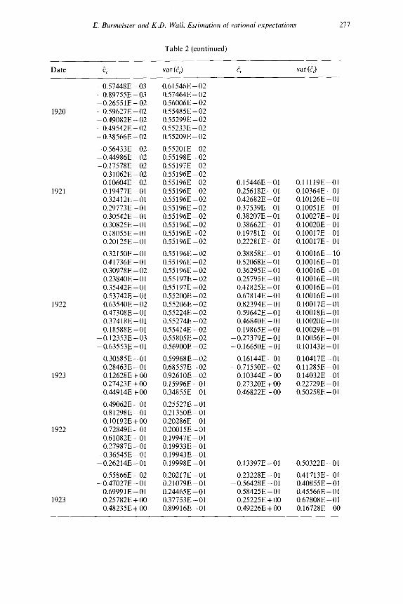
E. Burmeister and K.D. Wall, Estimation of rational expectations 277
Table 2 (continued)
Date
1920
1921
1922
1923
1922
1923
Ct var (2,) c, var (e,)
-0S7448E-03 -0.89755E-03 -0.26551E-02 -0.59627E-02 - 0.49082E - 02 - 0.49542E - 02 - 0.38566E ~ 02
0.61546E-02 0.57464E-02 0.56006E -02 0.55485E - 02 0.55299E-02 0.55233E -02 0.55209E-02
-0.56433E-02 0.552OlE-02 -0.44986E-02 0.55198E-02 -O.l7578E-02 0.55197E-02
0.31062E-02 0.55196E-02 O.l0604E-02 0.55196E-02 O.l9477E-01 0.55196E-02 0.32412E-01 0.55196E-02 0.297738 - 01 0.55196E-02 0.30542E - 01 0.55196E-02 0.30825E-01 0.55196E-02 O.l8055E-01 0.551968-02 0.20125E-01 0.55196E-02
0.32150E-01 0.41736E-01 0.30978E-02 0.23840E - 01 0.35442E-01 0.53742E-01 0.63540E - 02 0.47308E-01 0.37418E-01 O.l8588E-01
-O.l2353E-03 -0.63553F-01
0.30585E-01 0.28463E -01 O.l2628E+00 0.27423E +00 0,44914E+OO
0.55196E-02 0.55196E-02 0.55 196E - 02 0.55197E-02 0.55197E-02 0.55200E - 02 0.55206E -02 0.55224E - 02 0.55274E-02 0.55414E-02 0.55805E-02 _
0.569OOE -02 _
0.599688 - 02 0.685578 - 02 _
0.926108-02 O.l5996E-01 0.34855E-01
0.49062E - 01 0.81298E-01 0.10192E+OO 0.72849E - 01 0.61082E-01 0.27987E-01
-0,36545E-01 -0,26214E-01
0.25527E - 01 0.21350E-01 0.20286E - 01 0.20015E-01 O.l9947E-01 O.l9933E-01 O.l9943E-01 O.l9998E-01
0.55866E - 02 -0,47027E-01
0.69991E-01 0.25782E + 00 0.48235E + 00
0.20217E-01 0.21079E-01 0.24465E -01 0.37753E-01 0.89916E-01
O.l5446E-01 0.25618E-01 0.42682E - 01 0.375398-01 0.38207E-01 0.38662E-01 O.l9781E-01 0.22281E-01
0.38858E-01 0.52068E -01 0.36295E-01 0.25795E -01 0.41825E-01 0.678148-01 0.82394E - 01 0.59642E-01 0.46840E - 01 O.l9865E-01
-0.27379E-01 O.l6650E-01
O.l6144E-01 0,71530E-02 0.10344E + 00 0.27320E + 00 0.46822E + 00
O.l3397E-01
0.23228E - 01 ~0.56428E-01 0.58425E - 01 0.25225E + 00 0.49226E + 00
O.l1119E-01 O.l0364E-01 O.l0126E-01 O.l0051E-01 O.l0027E-01 O.l0020E-01 O.l0017E-01 O.l0017E-01
O.l0016E- 10 O.l0016E-01 O.l0016E-01 O.l0016E-01 O.l0016E-01 O.l0016E-01 O.l0017E-01 O.lOOlSE-01 O.l0020E-01 O.l0029E-01 O.l0056E-01 O.l0143E-01
O.l0417E-01 O.l1285E-01 O.l4032E-01 0.22729E - 01 0.50258E - 01
0.50322E - 01
0.41713E-01 0.40855E-01 0.45566E-01 0.67808E-01 O.l6728E-00
278 E. Burmeister and K.D. Wall, Estimation of rational expectations
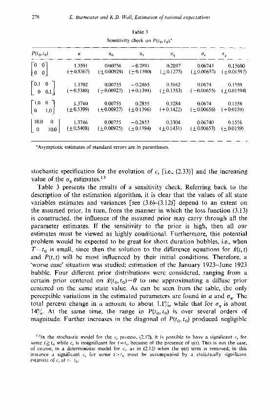
Table 3
Sensltlvlty check on P(t,, to).”
a a0 a1 ci4 0, 0,
1.3591 0.00756 - 0.2891 0.2897 0.06741 0.15600
(kO.5367) (kO.00929) (+_0.1390) (kO.1275) (~0.00657) (+0.01597)
1.3702 0.00755 -0.2865 0.3162 0.0674 0.1559
(+0.5388) (fO.00927) (kO.1394) (kO.1353) (+0.00655) (io.o1594) 1.3740 0.00755 -0.2855 0.3284 0.0674 0.1558
(k0.5399) (+0.00927) (k0.1396) (i0.1422) (+0.00656) (kO.0159)
1.3746 0.00755 -0.2853 0.3304 0.06740 0.1558 (kO.5408) (+0.00925) (k0.1394) (k0.1431) (+0.00653) (kO.0159)
“Asymptotic estimates of standard errors are in parentheses.
stochastic specification for the evolution of c, [i.e., (2.33)] and the increasing value of the CJ~ estimates.13
Table 3 presents the results of a sensitivity check. Referring back to the description of the estimation algorithm, it is clear that the values of all state variables estimates and variances [see (3.6)-(3.12)] depend to an extent on the assumed prior. In turn, from the manner in which the loss function (3.13) is constructed, the influence of the assumed prior may carry through all the parameter estimates. If the sensitivity to the prior is high, then all our estimates must be viewed as highly conditional. Furthermore, this potential problem would be expected to be great for short duration bubbles, i.e., when T--to is small, since then the solution to the difference equations for -i-(t, t) and P(t, t) will be most influenced by their initial conditions. Therefore, a ‘worse case’ situation was studied: estimation of the January 1923-June 1923
bubble. Four different prior distributions were considered, ranging from a certain prior centered on i(t,, to) =U to one approximating a diffuse prior
centered on the same state value. As can be seen from the table, the only perceptible variations in the estimated parameters are found in u and By. The total percent change in a amount to about l.l%, while that for crl is about 14%. At the same time, the range in P(t,, to) is over several orders of magnitude. Further increases in the diagonal of P(to, t,) produced negligible
131n the stochastic model for the c, process, (2.12), it is possible to have a significant q for some t> t, while c, is insignificant for t=t, because of the presence of p(t). This is not the case, of course, in a deterministic model for c,, as in (2.12) when the q(t) term is removed; in this instance a significant c, for some t>t, must be accompanied by a statistically significant estimate of c, at t = t,.

E. Burmeister and K.D. Wall, Estimation of rational expectations 279
variations in the parameter estimates. Sensitivity to the assumed prior does not appear to be a problem.
Fig. 1 depicts the trajectories of c, produced by application of the smoothing algorithm to the model with the parameters given in table 1. Table 2 presents the c, estimates plotted in this figure, together with the corresponding estimated error variances.
The presence of significant c, estimates in the stochastic case, prompted a further estimation of the model under a restriction corresponding to a deterministic evolution for the c,‘s. More specifically, the model was re-
0.5
0.4
0.3
0.2
0.1
0.0
-. 1
s X
0 Bubble beginning in Jan. 1919
x Bubble beginning in Oct. 1919
A Bubble beginning in Jul. 1920
P Bubble beginning in Jun. 1921
T Bubble beginning in Jun. 1922
t Bubble beginning in Jan. 1923
Fig. 1. Smoothed estimates for c, (stochastic)

Tab
le
4
Est
imat
ion
resu
lts
for
dete
rmin
istic
ca
se.
‘Bub
ble’
da
tes
a Q
-sta
tistic
” L
.M.
test
(l
slj4
)
l/19-
6/23
10/1
9-61
23
l/2&
6/23
6/21
-612
3
6122
-612
3
6123
-612
3
2.31
23
(k0.
4238
) 0.
0079
65
- 0.
3970
(k
O.0
0932
6)
(+0.
1241
1)
2.01
94
0.00
1919
-
0.38
45
(*0.
4151
) (k
O.0
0942
) (k
0.12
53)
1.82
53
(+0.
3914
) 0.
0018
64
- 0.
3699
(_
+0.0
0940
4)
(kO
.128
6)
1.41
10
(+ 0
.356
8)
0.00
778
-0.3
480
(+0.
0096
1)
(kO
.132
9)
0.98
48
( f. 0
.280
0)
0.00
166
-0.3
153
(+0.
0094
2)
(k0.
1361
)
0.59
88
(_+0
.251
0)
0.00
156
-0.2
888
(_+0
.009
28)
(kO
.139
8)
0.06
798
0.23
25
(+
0.00
666)
(+
0.
0262
)
0.06
188
0.22
59
(kO
.006
11)
(kO
.024
2)
0.06
778
0.21
89
(k0.
0068
1)
(fO
.023
1)
0.06
763
0.20
98
( + 0
.006
79)
( k 0
.022
9)
0.06
749
0.19
84
( & 0
.006
69)
( + 0
.020
8)
0.06
742
0.19
05
(kO
.006
56)
(f0.
0193
)
9.14
3(22
) 0.
2912
1.
0713
1.
1903
1.
9353
16.2
98(2
4)
9.80
5(22
) 0.
2741
1.
0352
1.
1267
1.
9151
15.6
35(2
4)
9.40
8(22
) 0.
2543
0.
9925
1.
0566
1.
8923
14.5
75(2
4)
9.21
5(22
) 0.
2252
0.
9276
0.
9599
1.
8594
13.7
80(2
4)
9.27
5(22
) 0.
1841
0.
8306
0.
8377
1.
8127
18.5
50(2
4)
9.54
0 (2
2)
0.15
30
0.15
26
0.75
71
1.71
68
6.09
5(24
)
“See
not
e b
to
tabl
e 1.

E. Burmeister and K.D. Wall, Estimation of rational expectations 281
Table 5
Smoothed estimates for cl and its error variance (deterministic case).
‘Bubble’ dates
t/19-6/23
10/19-6123
7/20-6123
612 t-6123
6122-6123
l/23-6/23
Cl” var(c,J CT
0.204 x IO-” 0.790 x lo-r8 0.3816
0.123 x lo-’ 0.273 x lo-r6 0.3903
0.916 x lo-’ 0.146 x lo-l4 0.4006
0.164 x 10m5 0.438 x 10-r’ 0.4170
0.991 x lo-4 0.147 x loms 0.4453
0.349 x lo-* 0.171 x 10⁻⁵ 0.4714
var (c~)
0.0277
0.0278
0.0279
0.0284
0.0297
0.0312
estimated with cr,, constrained to zero. If large estimates for eV led to insignificance of the q’s, as was the case for the last two bubbles, then restriction of CJ,, to zero should produce significant c, in all instances.
Tables 4 and 5 and fig. 2 summarize the results of this re-estimation. As in the previous estimation using the second-order money growth rate model,
(3.5) convergence of the iterative estimation procedure was achieved in each instance. In addition, all residual series passed their whiteness tests. Parameter estimates are given in table 4 and reveal an interesting variation in the estimates for a, CI~, and ep. Table 5 presents the smoothed estimates for the terminal and initial values of c,‘s and its estimation error variance.14 In each case the q’s are significant under the usual normal distribution assumption.
5. Conclusions
In summary, our empirical evidence strongly suggests that for this model it is impossible to maintain the common assumption that rational expectations
are always convergent. This conclusion is most disturbing in large part because it means that the actual price at each t may be indeterminate without some additional assumption to determine the c,‘s. One solution to this difficulty having considerable intuitive appeal to many economists involves a slow price adjustment mechanism which might determine the initial condition by p*(O, 0) =p(O), where p(O) is historically given. However, the issue of stochastic determinacy must be left as unresolved for now.
14Under the restriction of cr,=O, the smoothed estimates of cl and P,,(t, T) become mere backward extrapolations of a,(rr;T) and PII( Thus, the smoothed estimate of c, (tc7’) is obtained from i,(t, T)=(l+ l/a)‘~ra,(7; T) while the smoothed estimation error variance is obtained from Pl,(t, T)=(l+ I/a) ‘(‘~r)PI1(?; 7’). See Anderson and Moore (1979, pp. 187-190) or Jazwinski (1970, pp. 215-218) for details.

282 E. Burmeister and K.D. Wall, Estimation of rational expectations
0.:
0.4
0.3
0.2
0.1
0.0
-. 1
0 Bubble beginning in Jan. 1919
X Bubble beginning in Oct. 1919
A Bubble beginning in Jql. 1920
CI Bubble beginning in Jun. 1921
v Bubble beginning in Jun. 1922
+ Bubble beginning in Jan. 1923
St h
tl
0
iV
i?n oA +
1919 1920 1921 1922 1923
Fig. 2. Smoothed estimates for c, (deterministic).
It is important to recognize that the issues we have raised in this paper are not restricted to the simple monetary model of inflation studied here. The fact that identical conceptual issues arise in more complex rational expectations models of the Lucas-Sargent type is evident from the analysis of Burmeister (1980, 1982) and Burmeister, Flood and Turnovsky (1981).
Our preliminary work has left us with several unanswered questions. One should investigate whether or not the assumption of known and constant parameters is justified, and it is important to test alternative specifications for

E. Burmeister and K.D. Wall, Estimation of rational expectations 283
the money supply function which include, for example, the variable p*(t + 1, t). Likewise one might try alternative specifications for the stochastic c,
process. Our primary conclusion is that estimation techniques which impose
restrictions implied by the assumption of convergent expectations, and which therefore are conditional upon this convergent expectations assumption, are suspect without additional verification of the underlying stability hypothesis.
We have demonstrated the feasibility of an alternative estimation methodology which does not preclude the possibility that rationally formed expectations are unstable. We have shown how to test an important hypothesis and to obtain parameter estimates which are not conditional upon a perhaps invalid stability assumption.
References
Anderson, B.D.O. and J.B. Moore, 1979, Optimal filtering (Prentice-Hall, Englewood Cliffs, NJ). Black, Fischer, 1974, Uniqueness of the price level in monetary growth models with rational
expectations, Journal of Economic Theory, Jan. Box, George E.P. and Gwilym M. Jenkins, 1973, Time series analysis: Forecasting and control,
rev. ed. (Holden Day, San Francisco, CA). Bryson, A.E. and Y.-C. Ho, 1969, Applied optimal control (Blaisdell, Waltham, MA). Bucy, R.S. and P.D. Joseph, 1968, Filtering for stochastic processes with applications (Wiley,
New York). Burmeister, Edwin, 1980, On some conceptual issues in rational expectations modelling, Journal
of Money, Credit and Banking, Nov. Burmeister, Edwin, 1981, Indeterminacy and stability in both rational expectations and perfect
foresight models, Paper presented at Summer Econometric Society Meetings, San Diego, June (revised 1982).
Burmeister, Edwin, Robert P. Flood and Stephen J. Turnovsky, 1979, Rational expectations and stability in a stochastic monetary model of inflation, Working paper (University of Virginia, Charlottesville, VA).
Burmeister, Edwin, Robert P. Flood and Peter M. Garber, 1983, On the equivalence of solutions in rational expectations mode, Journal of Economic Dynamics and Control, forthcoming.
Caines, P.E., 1976, Prediction error methods for stationary stochastic processes, IEEE Transactions on Automatic Control AC-21, no. 4, Aug., 500-505.
Cooley, Thomas F., Barr Rosenberg and Kent D. Wall, 1977, A note on optimal smoothing for time varying coefficient problems, Annals of Eco. Sot. Meas. 6, no. 4.
Flood, Robert P. and Peter M. Garber, 1980, Market fundamentals vs. price level bubbles: The first tests, Journal of Political Economy 88, no. 4, Aug., 745-770.
Godfrey, L.G., 1978, Testing against general autoregressive and moving average error models when the regressors include lagged dependent variables, Econometrica 46, no. 6, Nov.
Goodrich, R.L. and Peter E. Caines, 1979, Linear system identification from nonstationary cross- sectional data, IEEE Transactions on Automatic Control AC-24, no. 3, June, 4033410.
Green, Jerry R. and Seppo Honkapohja, 1979, Variance minimizing monetary policies with lagged price adjustment and rational expectations, Discussion paper no. 721, Sept. (Harvard Institute of Economic Research, Cambridge, MA).
Hansen, Lars P. and Thomas J. Sargent, 1980, Formulating and estimating dynamic linear rational expectations models, Journal of Economic Dynamics and Control 2, no. 1, 746.
Jazwinski, A.H., 1970, Stochastic processes and tittering theory (Academic Press, New York). Ljung, Lennart, 1978. Convergence analysis of parametric identification methods, IEEE
Transactions on Automatic Control AC-23, 770-783.

284 E. Burmeister and K.D. Wall, Estimation qfrational expectations
Ljung, Lennart and Peter E. Caines, 1979, Asymptotic normality of prediction error estimators for approximate systems models, Stochastics 3, 29946.
McCallum, Bennett T., 1980, Rational expectations and macroeconomic stabilization policy: An overview, Journal of Money, Credit and Banking, Nov.
Muth, J.F., 1967, Rational expectations and the theory of price movements, Econometrica, July. Samuelson, Paul A., 1957, Intertemporal price equilibrium: A prologue to the theory of
speculation, Weltwirtschaftliches Archiv 79, no. 2. Reprinted in: Joseph E. Stiglitz, ed., 1966, The collected scientific papers of Paul A. Samuelson, Vol. 2 (M.I.T. Press, Cambridge, MA).
Samuelson, Paul A., 1967, Indeterminacy of developments in a heterogeneous-capital model with constant saving propensity, in: Karl Shell, ed., Essays on the theory optimal economic growth (M.I.T. Press, Cambridge, MA). Reprinted in: Robert C. Merton, ed., 1972, The collected scientific papers of Paul A. Samuelson, Vol. 3 (M.I.T. Press, Cambridge, MA).
Sargent, Thomas J. and Neil Wallace, 1973, Rational expectations and the dynamics of hyperinflation, International Economic Review 4, June.
Wall, Kent D., 1980, Generalized expectations modeling in econometrics, Journal of Economic Dynamics and Control 2, no. 2, May.