kansas geological survey - university of kansas
TRANSCRIPT

Central pivot irrigation system at which pumped water was discharged forHigh Plains aquifer pumping test in October of 2003.
Kansas Geological Survey
ANALYSIS OF TWO PUMPING TESTS AT THEO’ROURKE BRIDGE SITE ON THE ARKANSAS
RIVER IN PAWNEE COUNTY, KANSAS
James J. Butler, Jr., Donald O. Whittemore, Xiaoyong Zhan, and John M. Healey
Prepared for theKansas Department of Agriculture, Division of Water Resources
Kansas Geological Survey Open-File Report 2004-32June 2004

2

EXECUTIVE SUMMARY
Two multi-day pumping tests were performed by the Kansas Geological Survey at the
O’Rourke Bridge site adjacent to the Arkansas River in Pawnee County, Kansas, near the city of
Larned. The first test was performed in the alluvial aquifer of the Arkansas River over two days in
September of 2002, while the second test was performed in the High Plains aquifer over four days in
October of 2003. The major objectives of these tests were to obtain information about the hydraulic
and geochemical responses of the aquifers to extended periods of pumping, the degree of hydraulic
connection between the two aquifers, and the impact of pumping on streamflow in the Arkansas
River. An extensive network of observations wells was installed for the two tests using direct-push
electrical conductivity logging to delineate the stratigraphy and to select the intervals over which the
wells were screened. Pumping-induced changes in water level (drawdown) were measured using
both automatic and manual methods, and water samples were collected before, during, and after the
pumping tests. Type curve analyses were performed on the drawdown data from two observation
wells for each pumping test. The transmissivity and specific yield of the Arkansas River alluvial
aquifer estimated from the first test were 3800 ft2/d and 0.31, respectively. There was no indication
of vertical flow from the underlying High Plains aquifer during the test, so no information about the
hydraulic conductivity of the confining unit separating the two aquifers could be obtained. The
transmissivity and storage coefficient of the High Plains aquifer estimated from the second test were
5400 ft2/d and 1.7x10⁻⁴, respectively. The pumping in the High Plains aquifer induced flow from the
overlying alluvial aquifer, and the hydraulic conductivity of the confining unit separating the two
aquifers was estimated to be 7.0x10⁻³ ft/d. The parameter estimates obtained from both tests are
consistent with the geologic composition of the unconsolidated aquifers and confining unit.
The Arkansas River rarely flowed at the O’Rourke Bridge site during 2002 and 2003, so
these pumping tests could not provide direct information about the impact of nearby pumping on
the flow of the Arkansas River. Regardless, the chemistry data collected during the first test indicate
that pumping of the alluvial aquifer will draw in water from the Arkansas River. The results of the

2
second test indicate that pumping of the High Plains aquifer will induce downward movement of
water from the alluvial aquifer through the confining unit. Thus, pumping in the High Plains aquifer
in the vicinity of the O’Rourke Bridge would also be expected to impact flow in the Arkansas River,
but the timing and magnitude of that impact will be dramatically different from that for pumping
from a well in the alluvial aquifer located close to the stream.
The details of the well construction for the pumping well used in the second test are not
known. However, it appears that the gravel pack extends upward from the High Plains aquifer
through the confining unit to the alluvial aquifer, a common design for irrigation wells installed prior
to the last two decades. This design appears to have resulted in movement of water from the alluvial
aquifer to the High Plains aquifer through the gravel pack prior, during, and after the pumping test.
This flow through the gravel pack must always be considered when interpreting the results of
analyses of water samples collected in the vicinity of older irrigation wells in the High Plains aquifer.
3
INTRODUCTION
Two multi-day pumping tests were performed by the Kansas Geological Survey (KGS) atthe O’Rourke Bridge site adjacent to the Arkansas River in Pawnee County, Kansas, in Septemberof 2002 and October of 2003. The September 2002 (henceforth, S2002) test was directed atincreasing information about the hydraulic properties of the Arkansas River alluvial aquifer(henceforth, alluvial aquifer) and its relationship to the river. The October 2003 (henceforth,O2003) test was directed at increasing information about the hydraulic properties of both the HighPlains aquifer and the confining unit that separates the High Plains and alluvial aquifers at theO’Rourke Bridge site. These tests were done as part of a multi-year research effort of the KGSfocused on developing a better understanding of the nature of stream-aquifer interactions in themiddle reaches of the Arkansas River, the impact of irrigation pumping on stream flow, and the roleof phreatophytes in the hydrology of the riparian zones of Kansas rivers. The Division of WaterResources of the Kansas Department of Agriculture was the primary source of funding for thisproject. Some of the observation wells used for these tests were constructed with funds providedby the KGS and Groundwater Management District #5. Jim Butler of the Geohydrology Section ofthe KGS served as the principal investigator for the project.
REPORT OVERVIEW
The following report will be divided into three main sections: Preliminary SiteInvestigation, Pumping Test Procedures and Results, and Water Sampling and AnalysisProcedures and Results. The first section provides a site overview and descriptions of the direct-push electrical conductivity profiling method used to select screened intervals for the observationwells and the direct-push approach used to install those wells. The second section consists of adescription of the procedures used to perform and analyze the two pumping tests and aninterpretation of the results. The third section consists of a description of the field proceduresused for acquiring water samples for geochemical analyses and an interpretative discussion of theresults of those analyses.
PRELIMINARY SITE INVESTIGATION
Site Overview
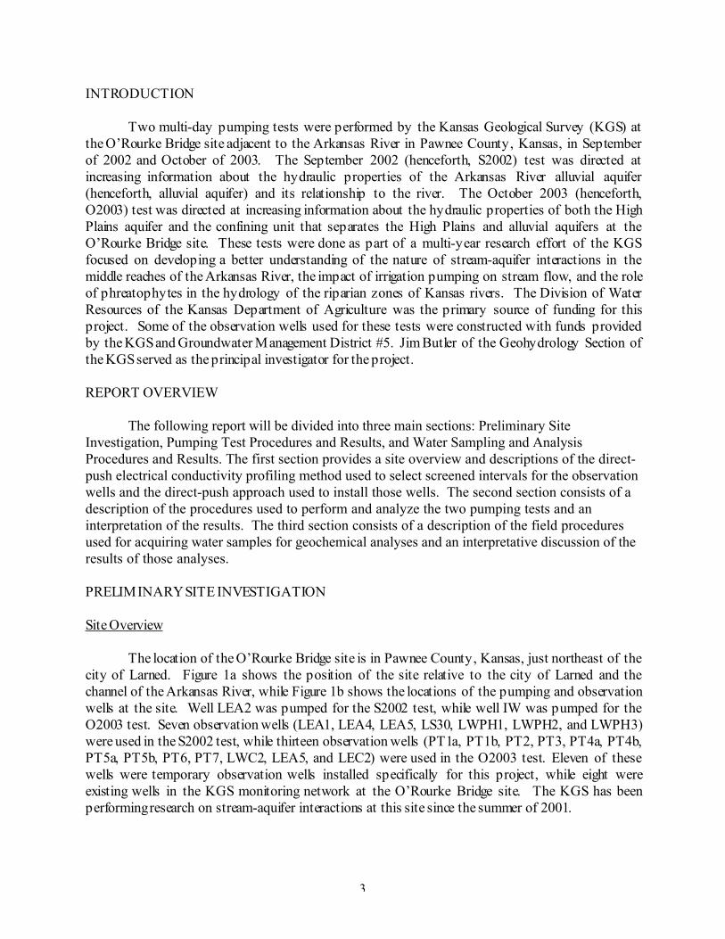
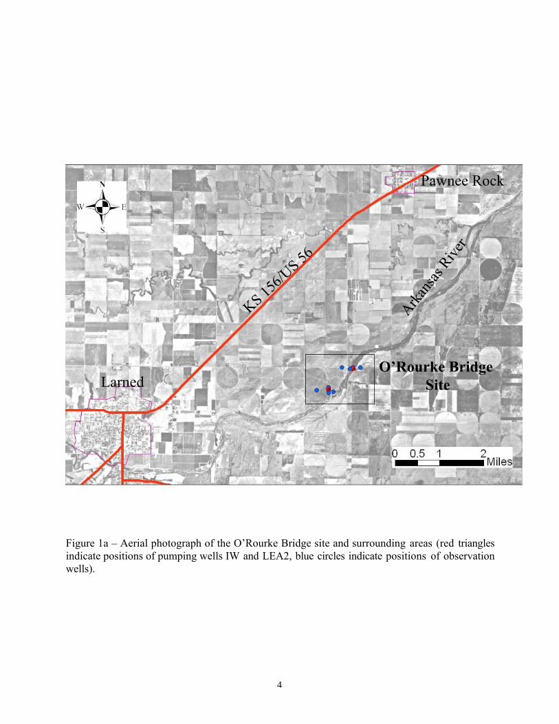
The location of the O’Rourke Bridge site is in Pawnee County, Kansas, just northeast of thecity of Larned. Figure 1a shows the position of the site relative to the city of Larned and thechannel of the Arkansas River, while Figure 1b shows the locations of the pumping and observationwells at the site. Well LEA2 was pumped for the S2002 test, while well IW was pumped for theO2003 test. Seven observation wells (LEA1, LEA4, LEA5, LS30, LWPH1, LWPH2, and LWPH3)were used in the S2002 test, while thirteen observation wells (PT1a, PT1b, PT2, PT3, PT4a, PT4b,PT5a, PT5b, PT6, PT7, LWC2, LEA5, and LEC2) were used in the O2003 test. Eleven of thesewells were temporary observation wells installed specifically for this project, while eight wereexisting wells in the KGS monitoring network at the O’Rourke Bridge site. The KGS has beenperforming research on stream-aquifer interactions at this site since the summer of 2001.
4
Larned
Pawnee Rock
KS 156/U
S 56
O’Rourke Bridge Site
Arkan
sas R
iver
Figure 1a – Aerial photograph of the O’Rourke Bridge site and surrounding areas (red trianglesindicate positions of pumping wells IW and LEA2, blue circles indicate positions of observationwells).
5
LWC2 LEC2
LWPH1
LWPH2LWPH3
LEA5LEA4LEA1LS30
LEA2
PT6 PT4A,B
PT3
PT2
PT1A,B
PT5A,B
PT7IW
Figure 1b – Aerial photo of well network at the O’Rourke Bridge site (red triangles indicatepositions of pumping wells IW and LEA2, blue circles indicate positions of observation wells).

6
Electrical Conductivity Profiling
The technique used in this project for stratigraphic delineation and selection of screenedintervals for the observation wells was a direct-push method commonly referred to as electrical-conductivity profiling (Christy et al., 1994; Butler et al., 1999; Schulmeister et al., 2003). Thisapproach is effective in defining subsurface lithology in unconsolidated alluvial sediments. Theelectrical-conductivity (EC) probe used in this work (Geoprobe SC 400) was designed such thatthe investigator can select different configurations to adjust the lateral extent of investigation. The configuration that gave the greatest lateral penetration (Wenner array) was used here.
The EC probe was advanced into the subsurface with a track-mounted Geoprobe 66DTunit using hydraulic pressure and a percussion hammer, while the electrical conductivity of thesubsurface was measured at intervals of 0.05 ft. In this work, the electrical conductivity of theunconsolidated sediments was assumed to be primarily a function of grain size. Thus, low valuesof electrical conductivity were assumed to indicate sand and gravel, intermediate values wereassumed to indicate silt, and high values were assumed to indicate clay. Although no cores weretaken to confirm the assumed relationships, previous work at a KGS research site in the KansasRiver floodplain has shown the general viability of these relationships (Butler et al., 1999;Schulmeister et al., 2003).
At most locations, the EC probe was advanced through the High Plains aquifer into theunderlying clay unit. At three locations where only shallow observation wells were planned, ECprofiling was terminated in the confining layer underlying the alluvial aquifer (observation wellsPT2 and PT7) or at a depth of six meters (LS30). The information obtained by the EC logs wasthe only means of lithologic interpretation used in this work because the well installationprocedure did not produce drill cuttings for visual inspection and description, and no cores weretaken.
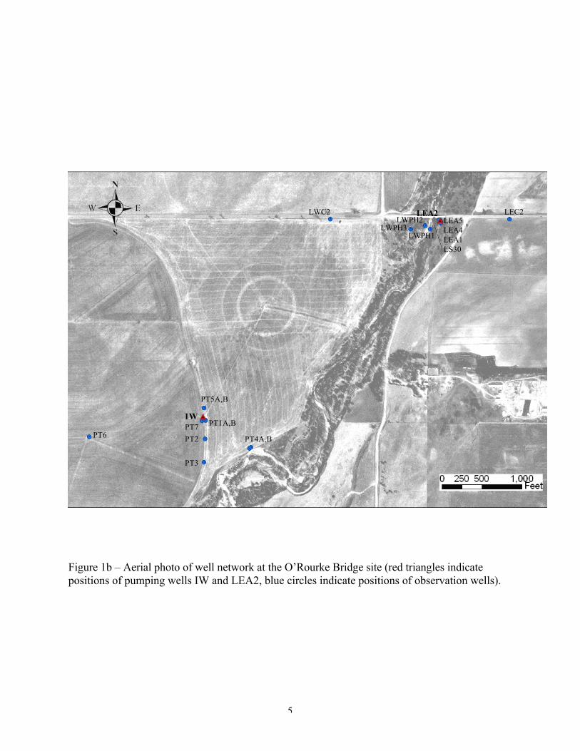
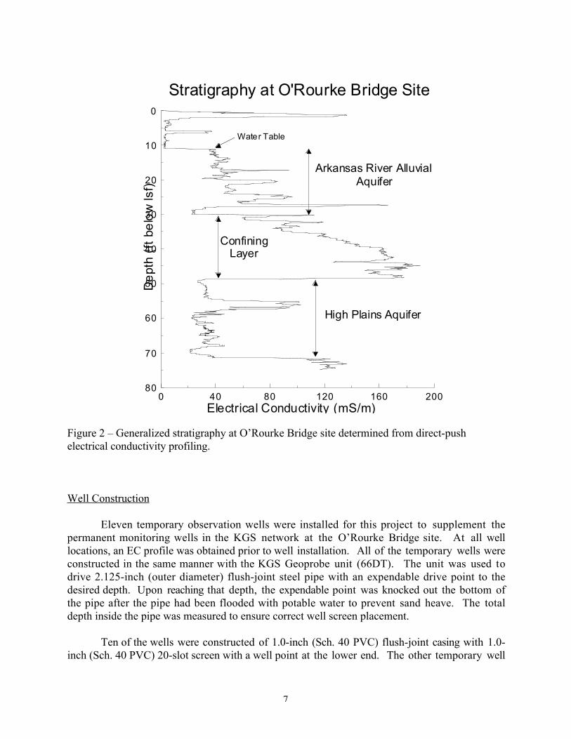
The direct-push electrical conductivity profile and interpreted stratigraphy for well nest PT1is shown in Figure 2. This profile, which is a reasonable representation of the stratigraphy acrossthe site, shows the three major units that exist in the shallow subsurface in the vicinity of theO’Rourke Bridge. The alluvial aquifer extends from the water table to the top of the confining layer,and is characterized by intermittent clay lenses, particularly in the lower two-thirds of its verticalextent. More details concerning this aquifer will be provided in the section on the S2002 test. Notethat the depth to the water table varies across the site from less than three feet immediately adjacentto the Arkansas River channel at well LWPH1 to over 11 feet at wells PT1 and PT5. The confininglayer was observed in all profiles obtained at the site. The thickness of the layer varies across thesite from 10.3 to 21.8 ft with no apparent directional pattern. The High Plains aquifer ischaracterized by intermittent clay lenses, particularly in its upper half. The thickness of sands inthe High Plains aquifer varies across the site from 9.6 to 22.4 ft with an apparent thinning on theeast side of the site.
7
0 40 80 120 160 200Electrical Conductivity (mS/m)
80
70
60
50
40
30
20
10
0
De
pth
(ft
belo
w ls
f)
Stratigraphy at O'Rourke Bridge Site
Water Table
High Plains Aquifer
Arkansas River Alluvial Aquifer
Confining Layer
Figure 2 – Generalized stratigraphy at O’Rourke Bridge site determined from direct-pushelectrical conductivity profiling.
Well Construction
Eleven temporary observation wells were installed for this project to supplement thepermanent monitoring wells in the KGS network at the O’Rourke Bridge site. At all welllocations, an EC profile was obtained prior to well installation. All of the temporary wells wereconstructed in the same manner with the KGS Geoprobe unit (66DT). The unit was used todrive 2.125-inch (outer diameter) flush-joint steel pipe with an expendable drive point to thedesired depth. Upon reaching that depth, the expendable point was knocked out the bottom ofthe pipe after the pipe had been flooded with potable water to prevent sand heave. The totaldepth inside the pipe was measured to ensure correct well screen placement.
Ten of the wells were constructed of 1.0-inch (Sch. 40 PVC) flush-joint casing with 1.0-inch (Sch. 40 PVC) 20-slot screen with a well point at the lower end. The other temporary well
8
(LS30) was constructed of 1.0-inch steel casing and screen. The casing string was assembled as itwas lowered through the center of the 2.125-inch pipe. After the casing string, with the screenand well point at its lower end, was lowered to the bottom, the pipe was retracted. Theunconsolidated formation collapsed back against the casing and screen as the pipe was removed.Retraction of the 2.125-in pipe continued until the bottom of the pipe string was adjacent to azone where an annular seal was necessary. Bentonite slurry was then poured into the annularspace between the inner diameter of the steel pipe and the outer diameter of the casing. After the2.125-inch pipe was removed from the hole, bentonite chips were poured into the borehole to fillthe remaining annular space to the land surface.
Tables 1 and 2 summarize well details for the temporary and permanent monitoring wellsused in this study. The thicknesses of the various units were determined from the EC logsassuming that electrical conductivity values less than 45-50 mS/m correspond to sands. Notethat as of the writing of this report, nine of the eleven temporary wells had been removed and theholes plugged.
Well Development
The completed wells were developed by airlifting with flow rates of over 10 gallons perminute. Development continued until groundwater turbidity was judged minimal. Slug testswere performed at all wells to assess the sufficiency of development activities. These testsdemonstrated that the wells were in good hydraulic connection with the aquifer in which theywere screened.

9
Table 1. Well construction and stratigraphy (from electrical conductivity logging) information forwells used in September 2002 pumping test.
Well
Welldepth,ft bls1
Wellradius,
f t2
Screenedinterval,
ft bls
Thickness of High
Plainsaquifer,
f t3
Thickness ofconfininglayer, ft
Thicknessof uppersand inalluvial
aquifer, ft
Thickness ofpossiblebarrier inalluvial
aquifer, ft
Total thicknessof
alluvial aquifer,f t4
Alluvial aquifer
LEA15 17.2 0.09 4.7-16.7
LEA25 16.5 0.17 11.4-16.2
LEA45 30.6 0.09 25.3-30.0
LWPH1 7.2 0.09 2.0-6.7 15.4 11.1 8.2 8.4 15.2
LWPH2 10.8 0.09 3.1-10.2 13.0 21.8 8.7 8.9 14.0
LWPH3 10.3 0.09 2.5-9.7 15.6 15.2 8.6 8.8 14.4
LS306 18.1 0.04 14-18 8.1
High Plains aquifer
LEA5 69.6 0.17 59.5-69.2 15.4 13.5 7.6 6.6 15.2
LEB7 13.4 10.3 ?8 8.8 ?8
1 - feet below land surface; 2 – inner diameter of casing and screen; 3 – thickness of sand intervals within theHigh Plains aquifer; 4 – thickness of sand intervals in alluvial aquifer, water table position measured within an 18-hr period prior to pumping test; 5 – electrical conductivity profiling not performed at this location (within 30 ft ofLEA5); 6 – electrical conductivity profiling terminated in possible barrier; 7 – electrical conductivity profiling only,no well – LEB located 436 ft to the east of LEA2; 8 – position of water table not known at time of test
Table 2. Well construction and stratigraphy (from electrical conductivity logging) information forobservation wells used in October 2003 pumping test.
WellWell depth,
ft bls1 Well
radius, ft2Screened
interval, ft blsThickness of HighPlains aquifer, ft3
Thickness ofconfining layer,
f t
Thickness ofalluvial aquifer,
f t4
Alluvial aquifer5
PT1b 28.1 0.04 12.9-22.7 8.0
PT2 24.4 0.04 14.1-24.0 10.4
PT4b 25.1 0.04 14.9-24.7 16.2
PT5b 29.8 0.04 19.6-29.4 12.0
PT76 24.9 0.04 14.6-24.5
High Plains aquifer7
PT1a 67.1 0.04 61.9-66.7 18.9 18.8
PT3 67.1 0.04 61.9-66.7 17.1 18.2 20.6
PT4a 67.1 0.04 61.9-66.7 15.1 13.1
PT5a 66.3 0.04 61.1-65.9 22.4 18.4
PT6 66.9 0.04 61.7-66.5 15.8 21.8 6.6
LWC2 71.6 0.17 61.7-70.8 21.3 12.4 11.9
LEA5 69.6 0.17 59.5-69.2 15.4 13.5 16.8
LEC2 71.8 0.17 66.2-71.2 9.6 13.8 20.4
1 - feet below land surface; 2 – inner diameter of casing and screen; 3 – thickness of sand intervals within theHigh Plains aquifer; 4 – thickness of sand intervals in alluvial aquifer, water-table position measured within an 18-

10
hr period prior to test; 5 – thickness of High Plains aquifer and confining unit only provided if not listedelsewhere; 6 – electrical conductivity profiling not performed at this well; 7 – thickness of alluvial aquifer onlyprovided if not listed elsewhere
11
PUMPING TESTS PROCEDURES AND RESULTS
Data Acquisition
Prior, during, and after both pumping tests, water levels were measured automatically with avariety of pressure transducers, and manually with electric tapes (Solinst and Heron). Use of thepressure transducers enabled changes in water levels to be monitored at a much higher frequencythan would be possible by manual means. The rate at which transducer readings were acquiredvaried between tests and, in the case of the O2003 test, between observation wells. For the S2002test, the rate varied from a measurement every second to a measurement every thirty seconds, withthe highest acquisition rate occurring at the start of the test and in the initial portion of the recoveryperiod. For the O2003 test, the rate varied from every 0.5 seconds to 5 minutes in the High Plainsaquifer wells, and from 0.5 seconds to 15 minutes in the alluvial aquifer wells. After cessation oftest monitoring, pressure measurement continued at the rate of a reading every 15 minutes in thepermanent wells of the KGS monitoring network.
Butler (1998) emphasizes the importance of checking transducer operation in the field. Forthis project, transducer operation was checked through an in-field calibration. This was done bycomparing pressure readings obtained with the transducers against electric tape measurements takenat the same time. The viability of a particular transducer was checked by performing a regression oftransducer-measured water-level changes versus manually measured changes, and assessing theregression coefficient and standard error of the regression relationship. Figure 3 shows a typicalregression relationship obtained through the in-field calibration. In this case, the relatively largestandard error was apparently produced by operator error in the electric tape measurements. Tables3 and 4 provide the sensor specifications and calibration results for the pressure transducers used inthe S2002 and O2003 tests, respectively. Note that absolute pressure sensors were utilized in bothtests, so atmospheric pressure was also recorded using a pressure sensor in the air column of amonitoring well at the site. The atmospheric pressure readings were subtracted from the records ofthe absolute pressure sensors prior to the regression analysis.
Additional measurements were made of pumping rate, precipitation, and water quality. Themethods for monitoring pumping rate differed between tests, so those methods are described in latersections. Precipitation data were acquired at the USGS gaging station at O’Rourke Bridge using anelectronic rain gauge. Water samples were periodically acquired during both tests as described inlater sections.
Arkansas River Flow During Study Period
The study was originally designed to assess the impact of groundwater pumping on theflow of the Arkansas River near Larned. The pumping test in the alluvial aquifer was performedin September 2002 (from the 17th to the 19th) as scheduled in the contract. Although there wasno flow in the river, the test provided data that were used to determine hydraulic and water-quality characteristics of the alluvial aquifer that could be used to assess the impact ofgroundwater pumping on the river if there had been flow. For example, the aquifer hydraulicproperties determined from the test could be inserted into a stream-aquifer interaction model topredict the impact of pumping from the alluvial aquifer on the river flow.

12
0 1 2 3 4 5 6 7 8 9 10 11Drawdown as measured by transducer (ft)
0
1
2
3
4
5
6
7
8
9
10
11
Dra
wdo
wn
as m
eas
ure d
by
elec
tric
tap
e (f
t)
Y = 0.999 * X - 0.001R-squared = 1.000Standard error = 0.046 ftNumber of observations = 74
Sensor 8215, 15 psig range
10/16-10/29/2003
Figure 3 – Results of in-field calibration of pressure transducer in well PT1a.
Table 3. Specifications and calibration results for pressure transducers used in S2002 pumpingtest.
WellTransducerSerial No.1
Transducer Range and
Type2CalibrationEquation3
AdjustedRegressionCoefficient
StandardError (ft)
Numberof
Observations
Alluvial aquifer
LEA1 5318 – IS/CS 20 psig y = 1.014x + 0.007 0.997 0.008 56
LEA4 1752 – IS/MT 15 psig y = 1.006x – 0.003 0.993 0.004 21
LWPH14 8338 – IS/MT 30 psia
LWPH24 6814 – IS/MT 30 psia
LWPH34 6613 – IS/MT 30 psia
LS30 5319 – IS/CS 20 psig y = 0.974x + 0.024 0.986 0.014 51
High Plains aquifer
LEA5 11424 – IS/MT 15 psig y = 0.984x - 0.034 0.999 0.014 19
1 – IS/CS – In-Situ transducer with Campbell-Scientific 23X datalogger, IS/MT – In-Situ MiniTroll integratedtransducer and data logger; 2 – psia – absolute pressure transducer, psig – gauge (relative to atmosphericpressure) pressure transducer; 3 – equation resulting from regression of transducer readings (x) versus electrictape measurements (y); 4 – drawdown was small at these wells and only four electric tape measurement wereobtained during monitoring so regression was not attempted, available data indicate sensors behaved in a linearfashion.

13
Table 4. Specifications and calibration results for pressure transducers used in O2003 pumpingtest.
WellTransducerSerial No.1
Transducer Range and
Type2CalibrationEquation3
AdjustedRegressionCoefficient
StandardError (ft)
Numberof
Observations
Alluvial aquifer
PT1b 8173 – IS/CS 15 psig y = 1.019x + 0.001 0.998 0.006 104
PT2 31149 - GW 13 psig y = 0.914x + 0.011 0.969 0.015 24
PT4b 31150 - GW 13 psig y = 0.936x + 0.016 0.995 0.009 37
PT5b 5318 – IS/CS 20 psig y = 0.977x – 0.006 0.991 0.009 104
PT7 44799 – S/LL 21.8 psia y = 0.904x – 0.005 0.983 0.010 9
High Plains aquifer
PT1a 8215 – IS/CS 15 psig y = 0.999x – 0.001 1.000 0.046 74
PT3 8484 – IS/MT 30 psig y = 0.997x – 0.004 0.999 0.028 84
PT4a 44775 – S/LL 21.8 psiay = 0.982x + 0.012y = 1.019x – 0.1915
0.9990.998
0.0160.040
3855
PT5a 5245 – IS/CS 10 psig y = 1.046x + 1.334 0.992 0.2146 56
PT6 8518 – IS/MT 30 psig y = 0.985x – 0.003 1.000 0.004 97
LWC2 4640 – IS/MT 30 psig y = 0.994x + 0.025 1.000 0.007 84
LEA5 11424 – IS/MT 15 psig y = 1.026x + 0.004 0.999 0.012 37
LEC2 4620 – IS/MT 30 psig y = 1.043x + 0.008 0.998 0.010 33
1 – IS/CS – In-Situ transducer with Campbell-Scientific 23X datalogger, IS/MT – In-Situ MiniTroll integratedtransducer and data logger, S/LL – Solinst Levelogger integrated transducer and datalogger, GW – Global Waterintegrated transducer and datalogger; 2 – psia – absolute pressure transducer, psig – gauge (relative toatmospheric pressure) pressure transducer; 3 – equation resulting from regression of transducer readings (x)versus electric tape measurements (y); 4 – only observations prior to pump cut off were used because ofapparent electrical noise after cutoff; 5 – apparent change in calibration relationship at 14:49:58 on 10/20/03 –reason for change is not known;6 – source of large error in transducer readings is not known; 7 - observations in first four hours of pumpingwere not used because of uncertainty regarding time at which electric tape measurements were obtained
The High Plains aquifer pumping test was delayed in hopes of performing the test duringa period of flow in the river. When it became apparent that there would not be sustained flow inthe river, the test was scheduled and performed on October 20-24, 2003.
The flow in the Arkansas River was continuous (up to 3 ft3/sec) from the beginning of2002 until April 17 (Figure 4). From April 18 to June 29, the river alternated between dry and amean daily flow of <0.7 ft3/sec (peak flow of <2 ft3/sec). Except for August 1-2, 2002, the riverwas dry from June 30, 2002 to September 8, 2003. A flow event occurred during September 9-25, 2003; the flow reached a peak of 174 ft3/sec and averaged 160 ft3/sec on September 16, 2003.The source of the flow was the Pawnee River, which received runoff from an intense rainstormover the tributary watershed of Buckner Creek and its tributary, Saw Log Creek. The ArkansasRiver remained dry from September 26 through the end of 2003.

14
1/1/02 4/2/02 7/2/02 10/1/02 1/1/03 4/2/03 7/2/03 10/1/03 1/1/04
0
4
8
12
16
20M
ean
dai
ly fl
ow, f
t3/s
ec
Figure 4. Mean daily flow of the Arkansas River at the O’Rourke Bridge during 2002-2003. Themean daily flow reached a peak of 160 ft3/sec during the flow event of September 2003.
September 2002 (S2002) Pumping Test
Well LEA2 (see Figure 1b) was pumped at an approximately constant rate of 23.0 gallonsper minute (gpm) from 8:40:35 on September 17, 2002 to 10:47:22 on September 19, 2002. Thetotal duration of the pumping period was 50.11 hours (180,407 secs). After the pump was cut off,water levels were monitored at all wells for another six hours, after which monitoring continued onlyin the permanent wells in the KGS network at the O’Rourke Bridge site. No precipitation occurredin the 48 hours prior to the test or during the pumping period. A small amount of precipitation(0.12 inches) occurred after the end of the test on September 19, but no further precipitation wasrecorded during the recovery period. Note that all clock times for the S2002 test are given in CentralDaylight Time.
The pumping rate was monitored using an electronic paddlewheel flowmeter (Omega FP-5800) connected to a datalogger (Campbell-Scientific 23X). The acquisition rate varied from ameasurement every second to a measurement every thirty seconds, with the highest acquisition rateoccurring at the start of the test. Flowmeter performance was manually checked at six times spaced
15
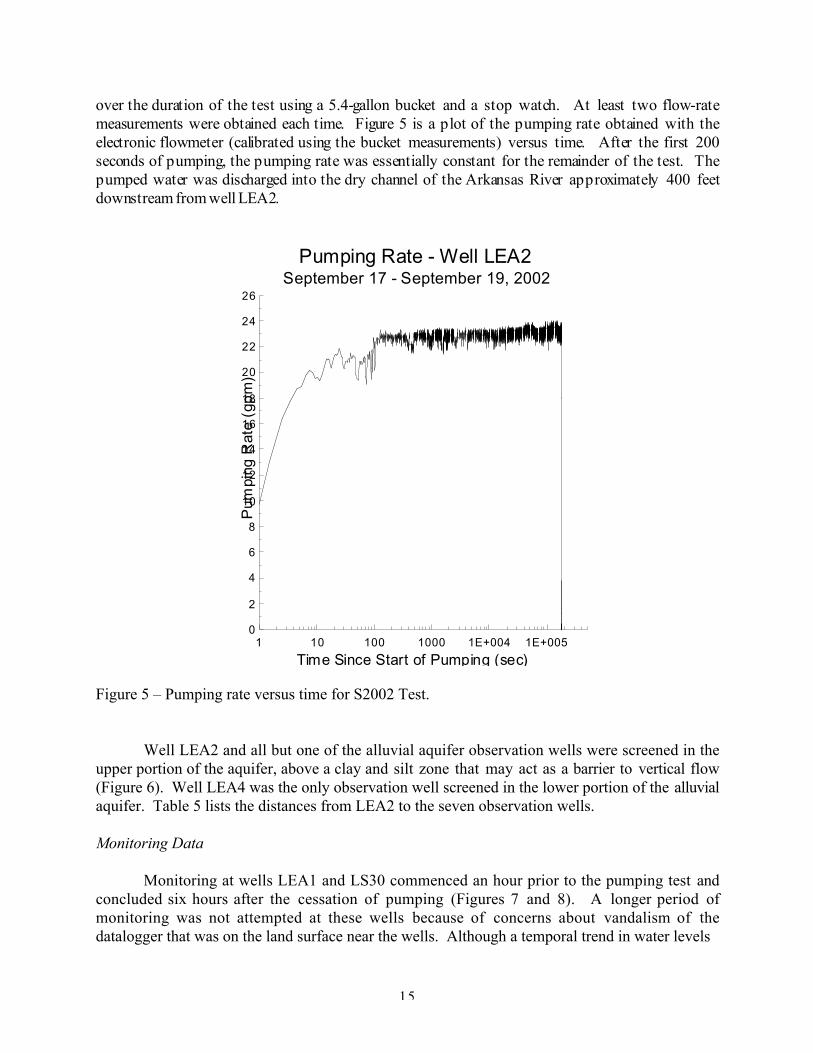
over the duration of the test using a 5.4-gallon bucket and a stop watch. At least two flow-ratemeasurements were obtained each time. Figure 5 is a plot of the pumping rate obtained with theelectronic flowmeter (calibrated using the bucket measurements) versus time. After the first 200seconds of pumping, the pumping rate was essentially constant for the remainder of the test. Thepumped water was discharged into the dry channel of the Arkansas River approximately 400 feetdownstream from well LEA2.
1 10 100 1000 1E+004 1E+005
Time Since Start of Pumping (sec)
0
2
4
6
8
10
12
14
16
18
20
22
24
26
Pum
ping
Rat
e (g
pm
) Pumping Rate - Well LEA2September 17 - September 19, 2002
Figure 5 – Pumping rate versus time for S2002 Test.
Well LEA2 and all but one of the alluvial aquifer observation wells were screened in theupper portion of the aquifer, above a clay and silt zone that may act as a barrier to vertical flow(Figure 6). Well LEA4 was the only observation well screened in the lower portion of the alluvialaquifer. Table 5 lists the distances from LEA2 to the seven observation wells.
Monitoring Data
Monitoring at wells LEA1 and LS30 commenced an hour prior to the pumping test andconcluded six hours after the cessation of pumping (Figures 7 and 8). A longer period ofmonitoring was not attempted at these wells because of concerns about vandalism of thedatalogger that was on the land surface near the wells. Although a temporal trend in water levels

16
0 20 40 60 80 100 120 140 160 180Electrical Conductivity (mS/m)
40
36
32
28
24
20
16
12
8
4
0
Dep
th (
ft b
elow
l sf )
Water Table
Sands
Sands
Possible Barrier
LEA4
LEA1
Pumping Well LEA2
Figure 6 – Expanded view of the shallow stratigraphy in the vicinity of the LEA well nest
Table 5. Distances from pumping well LEA2 to observation wells used in S2002 test.
1 - distances determined from surveying performed in March of 2004; 2 – screened below barrier in alluvialaquifer;3 – distance determined by tape measure in September of 2002
WellDistance from well
LEA2, ft1
Alluvial aquifer
LEA1 14.2
LEA42 18.1
LWPH1 161.0
LWPH2 198.0
LWPH3 384.6
LS30 30.33
High Plains aquifer
LEA5 16.5

17
9/17/02 9/18/02 9/19/02
Time
13
12.75
12.5
12.25
12
11.75
11.5
Dep
th t
o W
ate
r (f
t )
Well LEA1 Monitoring RecordSeptember 17 - September 19, 2002
Start of Pumping Test
End ofPumping Test
Figure 7 – Depth to water at well LEA1
9/17/02 9/18/02 9/19/02Time
13
12.75
12.5
12.25
12
11.75
11.5
Dep
th t
o W
ate
r (f
t )
Well LS30 Monitoring RecordSeptember 17 - September 19, 2002
Start of Pumping Test
End ofPumping Test
Figure 8 – Depth to water at well LS30

18
could not be determined from the monitoring record at these wells, a decline of approximately0.01 ft/day was estimated from the other wells in the alluvial aquifer. This magnitude of declinewould have a minimal effect on drawdown measured at wells LEA1 and LS30. Only the laterportion of the recovery data would be expected to be affected by the decline.
Monitoring at well LEA4 commenced the day prior to the pumping test and continuedafter the test as part of the KGS monitoring program (Figure 9). A temporal decline in waterlevel of approximately 0.01 ft per day can be observed in the data following the recovery period.The diurnal fluctuations in water level following the recovery period are a product ofphreatophyte activity (Butler et al., 2004). The rise in water level prior to the test isundoubtedly also a product of phreatophyte activity.
Monitoring at wells LWPH1, LWPH2, and LWPH3 started in August of 2002 andcontinued after the test as part of the KGS monitoring program (Figures 10 and 11). A temporaldecline in water level approaching 0.01 ft per day can also be observed in these data following therecovery period. The impact of the pumping test on well LWPH3 is barely discernible. In theother two wells, drawdown is discernible but the diurnal fluctuations produced by phreatophyteactivity introduce considerable noise into the drawdown data.
The monitoring record from the High Plains aquifer monitoring well (LEA5) indicates thatpumping activity in the High Plains aquifer made it difficult to discern any effects of pumping inthe alluvial aquifer (Figure 12). Drawdown due to pumping in the High Plains aquifer wasoccurring prior to the start of the pumping test and continued through the first 12 hours of thetest. At approximately 9 PM on 9/17, a well in the High Plains aquifer ceased pumping and thewater levels started to recover. Recovery continued until a well started pumping atapproximately 8 AM on 9/18. Drawdown continued until approximately 8 PM on 9/19, afterwhich water levels recovered until the end of the monitoring period.
Drawdown Analysis
Wells LEA1 and LS30 were chosen as the primary wells for use in the analysis becausethe magnitude of the drawdown at those wells was large compared to temporal trends andmeasurement noise. The Moench (1997) model for pumping tests in unconfined aquifers waschosen for the analysis of the drawdown data. The Moench model is an extension of the widelyused model of Neuman (1974). The major additions of the Moench model are the incorporationof wellbore storage at the pumping well and of non-instantaneous drainage of water from theunsaturated zone. In addition, the computational efficiency of the procedures used to evaluatethe mathematical functions is significantly improved over the model of Neuman. Theimplementation of the Moench model in AQTESOLV, an automated well-test analysis package(HydroSOLVE, 2001), was used here.
The analysis of the LEA1 data produced an excellent fit to the drawdown data (Figure 13)for a transmissivity (T) of 3740 ft2/day, a specific yield (Sy) of 0.16, and an anisotropy ratio(vertical component of hydraulic conductivity (Kz) over horizontal component of hydraulicconductivity (Kx)) of 0.06-0.2. The differences between the measured drawdown and the modelin the first 100 seconds of the test are due to mechanisms that are not included in the Moench

19
9/16/02 9/17/02 9/18/02 9/19/02 9/20/02 9/21/02 9/22/02 9/23/02Time
12.5
12.4
12.3
12.2
12.1
12
Dep
th t
o W
ate
r (f
t )
Well LEA4 Monitoring RecordSeptember 16 - September 23, 2002
Start of Pumping Test
End ofPumping Test
Figure 9 – Depth to water at well LEA4
9/16/02 9/17/02 9/18/02 9/19/02 9/20/02 9/21/02 9/22/02 9/23/02Time
3.7
3.6
3.5
3.4
3.3
Dep
th t
o W
ate
r (f
t )
Well LWPH1 Monitoring Record September 16 - September 23, 2002
Start of Pumping Test
End ofPumping Test
Figure 10 – Depth to water at well LWPH1

20
9/16/02 9/17/02 9/18/02 9/19/02 9/20/02 9/21/02 9/22/02 9/23/02Time
9.1
9
8.9
8.8
8.7
8.6
Dep
th t
o W
ate
r a
t LW
PH
2 ( f
t )
8.4
8.3
8.2
8.1
8
7.9
Dep
th t
o w
at e
r a t
LW
PH
3 (
f t)
LWPH2
LWPH3
LWPH2 and LWPH3 Monitoring Records September 16 - September 23, 2002
Start of Pumping Test
End ofPumping Test
Figure 11 – Depth to water at wells LWPH2 and LWPH3.
9/16/02 9/17/02 9/18/02 9/19/02 9/20/02 9/21/02 9/22/02Time
14
13.5
13
12.5
12
Dep
th t
o W
ate
r ( f
t )
Well LEA5 Monitoring RecordSeptember 17 - September 22, 2002
Start of Pumping Test
End ofPumping Test
Figure 12 – Depth to water at well LEA5.
21
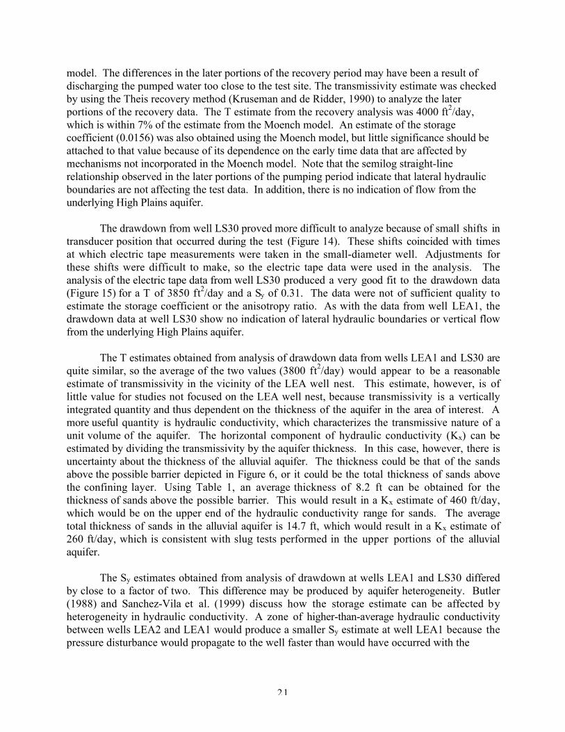
model. The differences in the later portions of the recovery period may have been a result ofdischarging the pumped water too close to the test site. The transmissivity estimate was checkedby using the Theis recovery method (Kruseman and de Ridder, 1990) to analyze the laterportions of the recovery data. The T estimate from the recovery analysis was 4000 ft2/day,which is within 7% of the estimate from the Moench model. An estimate of the storagecoefficient (0.0156) was also obtained using the Moench model, but little significance should beattached to that value because of its dependence on the early time data that are affected bymechanisms not incorporated in the Moench model. Note that the semilog straight-linerelationship observed in the later portions of the pumping period indicate that lateral hydraulicboundaries are not affecting the test data. In addition, there is no indication of flow from theunderlying High Plains aquifer.
The drawdown from well LS30 proved more difficult to analyze because of small shifts intransducer position that occurred during the test (Figure 14). These shifts coincided with timesat which electric tape measurements were taken in the small-diameter well. Adjustments forthese shifts were difficult to make, so the electric tape data were used in the analysis. Theanalysis of the electric tape data from well LS30 produced a very good fit to the drawdown data(Figure 15) for a T of 3850 ft2/day and a Sy of 0.31. The data were not of sufficient quality toestimate the storage coefficient or the anisotropy ratio. As with the data from well LEA1, thedrawdown data at well LS30 show no indication of lateral hydraulic boundaries or vertical flowfrom the underlying High Plains aquifer.
The T estimates obtained from analysis of drawdown data from wells LEA1 and LS30 arequite similar, so the average of the two values (3800 ft2/day) would appear to be a reasonableestimate of transmissivity in the vicinity of the LEA well nest. This estimate, however, is oflittle value for studies not focused on the LEA well nest, because transmissivity is a verticallyintegrated quantity and thus dependent on the thickness of the aquifer in the area of interest. Amore useful quantity is hydraulic conductivity, which characterizes the transmissive nature of aunit volume of the aquifer. The horizontal component of hydraulic conductivity (Kx) can beestimated by dividing the transmissivity by the aquifer thickness. In this case, however, there isuncertainty about the thickness of the alluvial aquifer. The thickness could be that of the sandsabove the possible barrier depicted in Figure 6, or it could be the total thickness of sands abovethe confining layer. Using Table 1, an average thickness of 8.2 ft can be obtained for thethickness of sands above the possible barrier. This would result in a Kx estimate of 460 ft/day,which would be on the upper end of the hydraulic conductivity range for sands. The averagetotal thickness of sands in the alluvial aquifer is 14.7 ft, which would result in a Kx estimate of260 ft/day, which is consistent with slug tests performed in the upper portions of the alluvialaquifer.
The Sy estimates obtained from analysis of drawdown at wells LEA1 and LS30 differedby close to a factor of two. This difference may be produced by aquifer heterogeneity. Butler(1988) and Sanchez-Vila et al. (1999) discuss how the storage estimate can be affected byheterogeneity in hydraulic conductivity. A zone of higher-than-average hydraulic conductivitybetween wells LEA2 and LEA1 would produce a smaller Sy estimate at well LEA1 because thepressure disturbance would propagate to the well faster than would have occurred with the

22
1 10 100 1000 10000 100000 1000000
Time Since Start of Pumping (sec)
0
0.2
0.4
0.6
0.8
Dra
wdo
wn
(ft
)
Drawdown data
Moench model
Well LEA1 Analysis - Moench Model September 17 - September 19, 2002
T = 3740 ft2 /daySy = 0.16
Kz/Kx?= 0.06-0.2
Figure 13 – Results of analysis of LEA1 drawdown data with Moench model
1 10 100 1000 10000 100000 1000000Time Since Start of Pumping (sec)
0
0.1
0.2
0.3
0.4
Dra
wdo
wn
(ft
)
Well LS30 DrawdownSeptember 17 - September 19, 2002
Shifts in Position of Transducer
Figure 14 – Noise in transducer measurements at well LS30.

23
average aquifer properties. Geochemistry data collected at the site are consistent with aninterpretation of a zone of higher conductivity between wells LEA1 and LEA2.
Drawdown data from well LEA4 were analyzed in an attempt to obtain more insight intothe appropriate values to use for Kx and Sy. As shown in Figure 6, well LEA4 was screenedbelow a zone that could serve as a barrier to vertical flow. This zone increased the complexity ofthe analysis because the Moench model does not incorporate heterogeneity in hydraulicconductivity. Thus, the fit was expected to be inferior to those obtained at wells LEA1 andLS30, particularly in the initial portion of the test and the recovery period. When the periodfrom 30,000 seconds to the end of the pumping test was emphasized in the analysis and the Testimate was assumed known (3800 ft2/day), a reasonable fit was obtained for the later portion ofthe pumping test (Figure 16). These results indicate that the full thickness of the aquifer shouldbe used to obtain the Kx estimate, and that the Sy value obtained from well LS30 is probably themore appropriate estimate for the specific yield. Note that the anisotropy ratio reflects theexistence of the possible barrier, but the quality of the data is not sufficient to have greatconfidence in that anisotropy estimate.
Summary
The results of the S2002 pumping test indicate that reasonable estimates for thetransmissivity and specific yield of the alluvial aquifer in the vicinity of well LEA2 are 3800ft2/day and 0.31, respectively. The T estimate corresponds to a hydraulic conductivity value of260 ft/day because the total thickness of sands in the alluvial aquifer appears to be contributingflow to the pumping well. The drawdown data show no indication of hydraulic boundaries orleakage from the underlying High Plains aquifer.
Unfortunately, there was no flow in the Arkansas River at the time of the S2002 pumpingtest. Without repeating the test when there is flow in the river, the nature of the relationshipbetween the alluvial aquifer and the Arkansas River cannot be unequivocally established. Despitethat, given the parameter estimates determined from the test, we can confidently state thatpumping near the Arkansas River will affect flow in the river. However, for pumping wellslocated more than a few hundred feet from the river, the timing of that impact will significantlylag the timing of the pumping because the relatively large value for specific yield will slow thepropagation of the pumping disturbance.
Trends in water levels, most likely produced by phreatophyte activity and pumping inthe High Plains aquifer, made it difficult to derive much insight from pumping-induced responsesin the more distant observation wells (LWPH1, LWPH2, and LWPH3). Repeating the testduring the early spring before phreatophyte activity and pumping in the High Plains aquifer havecommenced, and increasing the duration of the test would enable the drawdown at those wells tobe utilized in the analysis. Although the diameter of well LEA2 limits the size of the pump thatcan be used, a larger pump could be employed to increase the pumping rate by at least 50%, andtherefore improve the signal to noise ratio of the drawdown data at the more distant wells.

24
1 10 100 1000 10000 100000 1000000Time Since Start of Pumping (sec)
0
0.1
0.2
0.3
0.4
Dra
wdo
wn
(ft
)
Drawdown dataMoench model
Well LS30 Analysis - Moench Model September 17 - September 19, 2002
T = 3850 ft2/daySy = 0.31
Figure 15 - Results of analysis of LS30 drawdown data with Moench model.
1 10 100 1000 10000 100000 1000000Time Since Start of Pumping (sec)
0
0.05
0.1
0.15
0.2
Dra
wdo
wn
(ft
)
Drawdown data
Moench model
Well LEA4 Analysis - Moench Model September 17 - September 19, 2002
T = 3800 ft2/daySy = 0.30
Kz/Kx?= 0.002-0.006
Figure 16 – Results of analysis of LEA4 drawdown data with Moench model.

25
October 2003 (O2003) Pumping Test
Well IW was pumped beginning at 10:18:48 AM on October 20, 2003. The well waspumped for approximately 16 minutes to check operation and fill the subsurface pipe that extended1584 ft northeast to the central pivot irrigation system through which the water was discharged. The pump was shut down at 10:34:26 AM for repairs and to make final test preparations. Themain period of pumping began at 11:05:09 AM on October 20 and continued until 10:13:13 AM onOctober 24, 2003. The total duration of the main pumping period was 95.13 hours (342,484 secs). After the pump was cut off, water levels were monitored at all wells for another five to eighteendays, after which monitoring continued only in the permanent wells in the KGS network at theO’Rourke Bridge site. No precipitation occurred in the week prior to the test, during the pumpingperiod, or in the week following the cessation of pumping. Note that all clock times for the O2003test are given in Central Standard Time.
The pumping rate was monitored using an existing totalizing flowmeter mounted at the baseof the central pivot. The flowmeter was positioned near bends and a diameter change in thedischarge pipe, so the measurements were impacted by those features. Totalizer readings weretaken frequently in the first five hours of pumping in an attempt to record the rate variations early inthe test. Personnel from the Division of Water Resources measured the flow rate at three timesduring the test (afternoons of October 20 and 21, and morning of October 24) using an ultrasonicflowmeter (Panametrics PT868). Figure 17 is a plot of flow rate versus time for the entire period ofpumping that is based on a combination of the totalizer and ultrasonic flowmeter readings. Thepumping rate varied considerably in the first 4200 seconds but then was maintained at a nearconstant rate of 358 gpm until the last 20 seconds of the test when the pump motor wasinadvertently revved up prior to shut off.
1 10 100 1000 1E+004 1E+005Time Since Start of Pumping (sec)
0
100
200
300
400
500
600
700
800
Pum
pin
g R
ate
(g p
m)
Pumping Rate - Well IW October 20 - October 24, 2003
S tart of main pumping period
Figure 17 – Pumping rate versus time for O2003 test.

26
Well construction details for pumping well IW are not available, so the exact position ofthe screened interval within the High Plains aquifer is not known. Based on standardconstruction practices for irrigation wells at the time well IW was drilled, the radius of the screenis estimated to be 1.33 ft. The gravel pack is assumed to extend upward through the overlyingconfining unit into the alluvial aquifer, forming a conduit through the confining layer. The impactof this conduit will be discussed in later sections.
Figure 1b provides an areal view of the observation well network used in the O2003 testand Table 2 provides details concerning the construction of the individual observation wells. Allof the observation wells in the High Plains aquifer were screened in the middle to lower portionsof the aquifer (below 60 ft in Figure 2), and most of the observation wells in the alluvial aquiferwere screened across the middle portions of that unit (15-25 ft in Figure 2). Table 6 lists thedistances from pumping well IW to the 13 observation wells.
Table 6. Distances from pumping well IW to observation wells used in O2003 test
1 - distances determined from tape or calibrated wheel measurements in October of 2003; 2 – distancedetermined using tape measurements and March 2004 surveying data
Monitoring Data – High Plains aquifer wells
Monitoring at well PT1a began at 10:45 AM on October 16, 2003 and concluded at 12:15PM on November 11, 2003 (Figure 18). However, no data could be used beyond November 4because of datalogger malfunctioning. The malfunctioning may have been a result of mounting thedatalogger on a fence post through which electric current was run to constrain cattle in earlyNovember. No temporal trend could be detected in the data.
WellDistance from
pumping well, ft1
Alluvial aquifer
PT1b 55.2
PT2 276
PT4b 653
PT5b 115.8
PT7 47.9
High Plains aquifer
PT1a 54.2
PT3 564
PT4a 655
PT5a 115.7
PT6 1450
LWC2 2802
LEA5 38562
LEC2 45682

27
Monitoring at well PT3 began at 8:15 AM on October 16, 2003 and concluded at 11:45AM on November 11, 2003 (Figure 19). A very slight decline in water level (less than 0.05 ftover the entire monitoring period) was observed. This decline was ignored as it was very smallrelative to the drawdown and would only impact the later stages of the recovery data.
Monitoring at well PT4a began at 9:15 AM on October 16, 2003 and concluded at 2:45PM on November 11, 2003 (Figure 20). No temporal trend could be detected in the monitoringdata.
Monitoring at well PT5a began at 6:30 PM on October 15, 2003. However, the originalpressure transducer malfunctioned so the transducer was replaced and monitoring restarted on9:45 AM on October 20. Monitoring continued until 12:15 PM on November 11, 2003 butelectrical noise began to impact the data shortly after the pump was cut off on October 24(Figure 21). No data were available after October 30. The noise in the transducer readings isthought to have been caused by datalogger malfunctioning. A broken ground wire was found onOctober 29, consistent with the noise that was observed in the data.
Monitoring at well PT6 began at 12:30 PM on October 16, 2003 and concluded at 2:10PM on October 29, 2003 (Figure 22). Monitoring was concluded at that time because cattle werereleased into the pasture in which well PT6 was located, so the equipment was removed toprevent damage. A pronounced increase in water level was observed in well PT6 over the courseof the monitoring period. The cause of this increase could not be determined.
Monitoring at well LWC2 began in 2001 and continued after the test as part of the KGSmonitoring program (Figure 23). A small increase in water level was observed over themonitoring period, as were the effects of nearby pumping activity.
Monitoring at well LEA5 began in September of 2002 and continued after the test as partof the KGS monitoring program (Figure 24). A small increase in water level was again observedover the monitoring period, as were the effects of nearby pumping activity.
Monitoring at well LEC2 began in 2001 and continued after the test as part of the KGSmonitoring program (Figure 25). The impact of nearby pumping activity is very clearlydisplayed in the monitoring record of well LEC2. The impact of this activity diminished to thesouth and west (Figures 18-24), so it was assumed that the pumping activity was occurring tothe north and east of the O’Rourke Bridge site. The locations of the pumping wells that areresponsible for the features noted on Figure 25 could not be determined.

28
10/14/03 10/21/03 10/28/03 11/4/03Time
28
27
26
25
24
23
22
21
20
19
18
17
16
15
Dep
th t
o W
ate
r ( f
t)
Well PT1a Monitoring Record October 16 - November 4, 2003
Figure 18 – Depth to water at well PT1a.
10/14/03 10/21/03 10/28/03 11/4/03 11/11/03Time
20
19
18
17
16
15
14
Dep
th t
o W
ate
r ( f
t )
Well PT3 Monitoring Record October 16 - November 11, 2003
Figure 19 – Depth to water at well PT3.

29
10/14/03 10/21/03 10/28/03 11/4/03 11/11/03Time
20
19.5
19
18.5
18
17.5
17
16.5
16
15.5
15
Dep
th t
o W
ate
r (f
t )
Well PT4a Monitoring Record October 16 - November 11, 2003
Figure 20 – Depth to water at well PT4a.
10/14/03 10/21/03 10/28/03 11/4/03Time
24
23
22
21
20
19
18
17
16
15
14
Dep
th t
o W
ate
r ( f
t)
Well PT5a Monitoring Record October 20 - October 30, 2003
Electrical noise
Transducer replaced
Figure 21 – Depth to water at well PT5a.

30
10/14/03 10/21/03 10/28/03Time
16.4
16.2
16
15.8
15.6
De
pth
to
Wat
er (
f t)
Well PT6 Monitoring Record October 16 - October 29, 2003
Figure 22 – Depth to water at well PT6.
10/14/03 10/21/03 10/28/03 11/4/03 11/11/03Time
15
14.5
14
13.5
13
12.5
Dep
th t
o W
ate
r ( f
t )
Well LWC2 Monitoring Record October 14 - November 12, 2003
Figure 23 – Depth to water at well LWC2.

31
10/14/03 10/21/03 10/28/03 11/4/03 11/11/03Time
14.5
14
13.5
13
12.5
Dep
th t
o W
ate
r (f
t)
Well LEA5 Monitoring Record October 14 - November 12, 2003
Figure 24 – Depth to water at well LEA5.
10/14/03 10/21/03 10/28/03 11/4/03 11/11/03Time
17
16.5
16
15.5
De
pth
to W
ater
(ft
)
Well LEC2 Monitoring Record October 14 - November 12, 2003
Nearby pumping
Nearbypumping
Drawdown due to pumping test
Figure 25 – Depth to water at well LEC2.

32
Monitoring Data – alluvial aquifer wells
Monitoring at well PT1b began at 10:45 AM on October 16, 2003 and concluded at 12:15PM on November 11, 2003 (Figure 26). However, no data could be used beyond November 6because of datalogger malfunctioning (see discussion of well PT1a data). A definite decline inwater level could be observed in the monitoring data prior to the test. However, the electricalnoise that appeared to begin shortly after the pump was cut off made it difficult to relate the pre-and post-pumping trends.
Monitoring at well PT2 began at 8:30 AM on October 16, 2003 and concluded at 11:22AM on November 11, 2003 (Figure 27). A definite linear decline in water level can be observedprior to and immediately after the pumping test. A deviation from that trend is observed duringthe period of the pumping test. In late October, the water levels deviated from this trend as aresult of nearby pumping activity.
Monitoring at well PT4b began at 8:45 AM on October 16, 2003 and concluded at 2:27PM on November 11, 2003 (Figure 28). A definite linear decline in water level can be observedthrough the period during which the pumping test occurred, but the impact of the pumping isdifficult to discern. In late October, the water levels deviated from this trend as a result of nearbypumping activity in a manner similar to that observed at well PT2.
Monitoring at well PT5b began at 6:30 PM on October 15, 2003 and concluded at 12:15PM on November 11, 2003 (Figure 29). Electrical noise began to impact the data shortly afterthe pump was cut off on October 24. No data were available from 5:30 PM on October 30 until11:15 AM on November 6. The noise in the transducer readings and the missing data are thoughtto have been caused by datalogger malfunctioning (see discussion of well PT5a data).
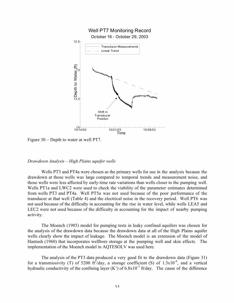
Monitoring at well PT7 began at 9:30 AM on October 16, 2003 and concluded at 1:45PM on October 29, 2003 (Figure 30). Monitoring was concluded at that time because cattle werereleased into the pasture in which well PT7 was located. A definite decline in water level couldbe observed in the monitoring data prior to the test. An apparent shift in the position of thetransducer at approximately 4:00 PM on October 21 made it difficult to relate the pre- and post-pumping trends. The cause of that shift could not be determined.

33
10/14/03 10/21/03 10/28/03 11/4/03Time
14
13.9
13.8
13.7
13.6
13.5
13.4
13.3
13.2
13.1
13
Dep
th t
o W
ate
r ( f
t )
Transducer MeasurementsLinear Trend
Well PT1b Monitoring Record October 16 - November 6, 2003
Electrical noise
Figure 26 – Depth to water at well PT1b.
10/14/03 10/21/03 10/28/03 11/4/03 11/11/03Time
12.5
12
11.5
11
Dep
th t
o W
ate
r ( f
t)
Transducer MeasurementsLinear Trend
Well PT2 Monitoring Record October 16 - November 11, 2003
Pump On
Pump Off
Figure 27 – Depth to water at PT2.

34
10/14/03 10/21/03 10/28/03 11/4/03 11/11/03Time
12.5
12
11.5
11
Dep
th t
o W
ate
r (f
t )
Transducer Measurements
Linear Trend
Well PT4b Monitoring Record October 16 - November 11, 2003
Pump On
Pump Off
Figure 28 – Depth to water at well PT4b.
10/14/03 10/21/03 10/28/03 11/4/03 11/11/03Time
15
14.5
14
13.5
Dep
th t
o W
ate
r ( f
t)
Transducer Measurements
Linear Trend
Well PT5b Monitoring Record October 16 - November 10, 2003
Missing data due to datalogger problems
Figure 29 – Depth to water at well PT5b.
35
10/14/03 10/21/03 10/28/03Time
14
13.5
13
12.5
Dep
th t
o W
ate
r (f
t)
Transducer MeasurementsLinear Trend
Well PT7 Monitoring Record October 16 - October 29, 2003
Shift inTransducer Position
Figure 30 – Depth to water at well PT7.
Drawdown Analysis – High Plains aquifer wells
Wells PT3 and PT4a were chosen as the primary wells for use in the analysis because thedrawdown at those wells was large compared to temporal trends and measurement noise, andthose wells were less affected by early-time rate variations than wells closer to the pumping well.Wells PT1a and LWC2 were used to check the viability of the parameter estimates determinedfrom wells PT3 and PT4a. Well PT5a was not used because of the poor performance of thetransducer at that well (Table 4) and the electrical noise in the recovery period. Well PT6 wasnot used because of the difficulty in accounting for the rise in water level, while wells LEA5 andLEC2 were not used because of the difficulty in accounting for the impact of nearby pumpingactivity.
The Moench (1985) model for pumping tests in leaky confined aquifers was chosen forthe analysis of the drawdown data because the drawdown data at all of the High Plains aquiferwells clearly show the impact of leakage. The Moench model is an extension of the model ofHantush (1960) that incorporates wellbore storage at the pumping well and skin effects. Theimplementation of the Moench model in AQTESOLV was used here.
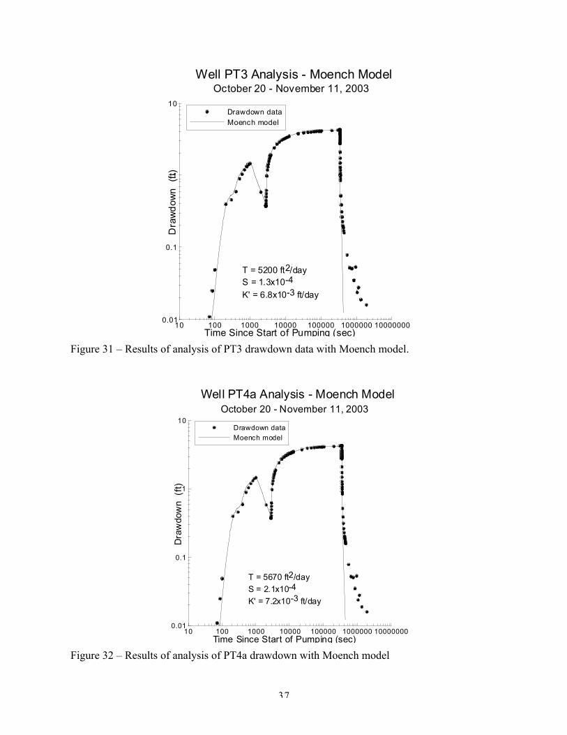
The analysis of the PT3 data produced a very good fit to the drawdown data (Figure 31)for a transmissivity (T) of 5200 ft2/day, a storage coefficient (S) of 1.3x10⁻⁴, and a verticalhydraulic conductivity of the confining layer (K’) of 6.8x10⁻³ ft/day. The cause of the difference

36
between the measured drawdown and the model in the later portions of the recovery could not bedetermined. However, nearby pumping activity is the most likely explanation. The significantrole of leakage during the test made it impossible to check the T estimate using the Theisrecovery method as was done with the S2002 test. Note that the K’ value is based on an averagethickness for the confining layer of 17.1 ft (average of all wells in Table 2 except LEA5 andLEC2).
The analysis of the PT4a data produced a very good fit to the drawdown data (Figure 32)for a T of 5670 ft2/day, a S of 2.1x10⁻⁴, and a K’ of 7.2x10⁻³ ft/day. The difference between themeasured drawdown and the Moench model in the later portions of the recovery period is againmost likely a product of nearby pumping activity.
The agreement between the parameter estimates obtained from the analysis of drawdowndata from wells PT3 and PT4a is quite good, so the averages of these values would appear to bereasonable estimates of the hydraulic properties of the High Plains aquifer and confining layer inthe vicinity of pumping well IW. Those averages are 5440 ft2/day (T), 1.7x10⁻⁴ (S), and 7.0x10⁻³
ft/day (K’). The average thickness of the High Plains aquifer in the vicinity of well IW is 18.4 ft(average of all wells from Table 2 except LEA5 and LEC2), so the transmissivity estimateequates to a hydraulic conductivity value of 295 ft/day. The storage coefficient equates to aspecific storage value of 9.2x10⁻⁶ ft-1. These estimates are both reasonable values for a coarsesand and gravel aquifer.
The viability of these estimates was assessed using drawdown from wells PT1a andLWC2. Type curves were generated using the average parameters determined from wells PT3and PT4a and then compared to the drawdown data. The type curve for PT1a underpredictedthe drawdown at that well (Figure 33). A good fit was obtained with the test data by decreasingthe T to 4710 ft2/day. Note that the variations in drawdown during the first 3000 seconds of thetest are a product of the rate variations shown in Figure 17, which are largely damped out at themore distant observation wells.
The type curve for LWC2 was lagged in response to the drawdown data at early timesbut produced a reasonable match at later times until nearby pumping activity began to impact thetest data (Figure 34). A closer match was obtained with the test data by increasing the T to 6580ft2/day and decreasing K’ to 5.9x10⁻³ ft/day. However, even in that case, nearby pumpingactivity impacted the match after approximately the first day of the test.
Given that the comparisons with the average parameters were not bad at wells PT1a andLWC2 and that the comparisons could be improved by adjusting parameter values by 20% orless, the average parameters obtained at wells PT3 and PT4a were considered reasonableestimates of the hydraulic parameters in the vicinity of well IW. Note that if individual Testimates are considered, there is an apparent increase in transmissivity with distance from wellIW – well PT1a (4710 ft2/day), well PT3 (5200 ft2/day), PT4a (5670 ft2/day), and LWC2 (6580ft2/day). Further work would be necessary to assess if that increase is a product of an increase inhydraulic conductivity or thickness of the High Plains aquifer, or due to some artifact of theanalysis.
37
10 100 1000 10000 100000 1000000 10000000Time Since Start of Pumping (sec)
0.01
0.1
1
10
Dra
wd
own
(f
t)
Drawdown dataMoench model
Well PT3 Analysis - Moench Model October 20 - November 11, 2003
T = 5200 ft2/dayS = 1.3x10⁻⁴
K' = 6.8x10⁻³ ft/day
Figure 31 – Results of analysis of PT3 drawdown data with Moench model.
10 100 1000 10000 100000 1000000 10000000Time Since Start of Pumping (sec)
0.01
0.1
1
10
Dra
wdo
wn
(ft
)
Drawdown dataMoench model
Well PT4a Analysis - Moench Model October 20 - November 11, 2003
T = 5670 ft2/day
S = 2.1x10⁻⁴
K' = 7.2x10⁻³ ft/day
Figure 32 – Results of analysis of PT4a drawdown with Moench model

38
1 10 100 1000 10000 100000 1000000Time Since Start of Pumping (sec)
0.01
0.1
1
10
100
Dra
wdo
wn
(ft
)
Drawdown dataMoench model
Well PT1a Analysis - Moench Model October 20 - November 4, 2003
T = 5440 ft2/day
S = 1.7x10⁻⁴
K' = 7.0x10⁻³ ft/day
Figure 33 – Comparison of drawdown data from PT1a with type curve based on the averageparameters from analysis of PT3 and PT4a.
100 1000 10000 100000 1000000Time Since Start of Pumping (sec)
0.01
0.1
1
10
Dra
wdo
wn
(ft
)
Drawdown dataMoench model
Well LWC2 Analysis - Moench Model October 20 - November 11, 2003
T = 5440 ft2/dayS = 1.7x10⁻⁴
K' = 7.0x10⁻³ ft/day
Figure 34 – Comparison of drawdown data from LWC2 with type curve based on the averageparameters from analysis of PT3 and PT4a.
39
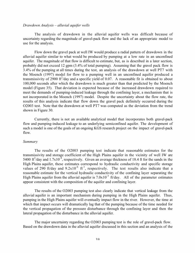
Drawdown Analysis – alluvial aquifer wells
The analysis of drawdown in the alluvial aquifer wells was difficult because ofuncertainty regarding the magnitude of gravel-pack flow and the lack of an appropriate model touse for the analysis.
Flow down the gravel pack at well IW would produce a radial pattern of drawdown in thealluvial aquifer similar to what would be produced by pumping at a low rate in an unconfinedaquifer. The magnitude of that flow is difficult to estimate, but, as is described in a later section,probably did not exceed 12 gpm (3.4% of total pumping). Assuming that the gravel pack flow is3.4% of the pumping at all times during the test, an analysis of the drawdown at well PT7 withthe Moench (1997) model for flow to a pumping well in an unconfined aquifer produced atransmissivity of 2900 ft2/day and a specific yield of 0.07. A reasonable fit is obtained to about100,000 seconds after which the drawdown is much greater than that predicted by the Moenchmodel (Figure 35). That deviation is expected because of the increased drawdown required tomeet the demands of pumping-induced leakage through the confining layer, a mechanism that isnot incorporated in the Moench (1997) model. Despite the uncertainty about the flow rate, theresults of this analysis indicate that flow down the gravel pack definitely occurred during theO2003 test. Note that the drawdown at well PT7 was computed as the deviation from the trendshown in Figure 30.
Currently, there is not an available analytical model that incorporates both gravel-packflow and pumping-induced leakage to an underlying semiconfined aquifer. The development ofsuch a model is one of the goals of an ongoing KGS research project on the impact of gravel-packflow.
Summary
The results of the O2003 pumping test indicate that reasonable estimates for thetransmissivity and storage coefficient of the High Plains aquifer in the vicinity of well IW are5400 ft2/day and 1.7x10⁻⁴, respectively. Given an average thickness of 18.4 ft for the sands in theHigh Plains aquifer, these estimates correspond to hydraulic conductivity and specific storagevalues of 290 ft/day and 9.2x10⁻⁶ ft-1, respectively. The test results also indicate that areasonable estimate for the vertical hydraulic conductivity of the confining layer separating theHigh Plains aquifer from the alluvial aquifer is 7.0x10⁻³ ft/day. All of the parameter estimatesappear consistent with the composition of the aquifer and confining layer.
The results of the O2003 pumping test also clearly indicate that vertical leakage from thealluvial aquifer is an important mechanism during pumping in the High Plains aquifer. Thus,pumping in the High Plains aquifer will eventually impact flow in the river. However, the time atwhich that impact occurs will dramatically lag that of the pumping because of the time needed forthe vertical propagation of the pressure disturbance through the confining layer and then thelateral propagation of the disturbance in the alluvial aquifer.
The major uncertainty regarding the O2003 pumping test is the role of gravel-pack flow. Based on the drawdown data in the alluvial aquifer discussed in this section and an analysis of the

40
geochemical data discussed in a later section, it is apparent that gravel-pack flow occurred duringthe pumping test. This flow was not great enough to have a major impact on the analysis ofdrawdown in the High Plains aquifer wells. However, gravel-pack flow should decrease the lagbetween pumping in the High-Plains aquifer and its impact on flow in the Arkansas River. Itshould also increase the magnitude of that impact. Further work is clearly needed to assess theimpact of gravel-pack flow under both pumping and non-pumping conditions. Ongoing researchat the KGS is addressing that issue.
10 100 1000 10000 100000 1000000Time Since Start of Pumping (sec)
0.01
0.1
1
Dra
wdo
wn
(f
t)
Drawdown dataMoench model
Well PT7 Analysis - Moench Model October 20 - October 29, 2003
T = 2900 ft2/daySy = 0.07
Figure 35 – Results of analysis of PT7 drawdown data with Moench (1997) model for flow to apumping well in an unconfined aquifer
41
WATER SAMPLING AND ANALYSIS PROCEDURES AND RESULTS
The objective of the water-quality investigations was to determine changes in thechemistry of the pumped water and evaluate their relationships to the groundwater and river-water chemistry as another approach to assessing the impact of pumping on Arkansas River flownear Larned.
Procedures
Water samples were periodically collected from the pumping well during both pumpingtests (Tables 7 and 8). Temperature and specific conductance were monitored in the field for theS2002 test, and conductance was recorded in the field during the first day of the O2003 test. Theco-author of this report who prepared this section was stationed at the center pivot to recordflowmeter readings during the first few hours of the O2003 pumping test. The center pivot islocated 1584 ft from the irrigation well, so the temperature of the water at the center pivot didnot reflect the temperature of the aquifer ground water and thus was not recorded. Watersamples were also collected three months after the O2003 pumping test from two pairs ofshallow and deep observation wells (sites PT1 and PT5) located near the irrigation well (Table 9). Profiles of specific conductance were recorded in observation wells PT1a, PT1b, and PT5b inNovember 2003, and in PT1b, PT2, PT3, PT4a and 4b, and PT5b in February 2003. Table 10 isa summary of the conductance values calculated or estimated as the mean for the screened intervalof the observation wells.
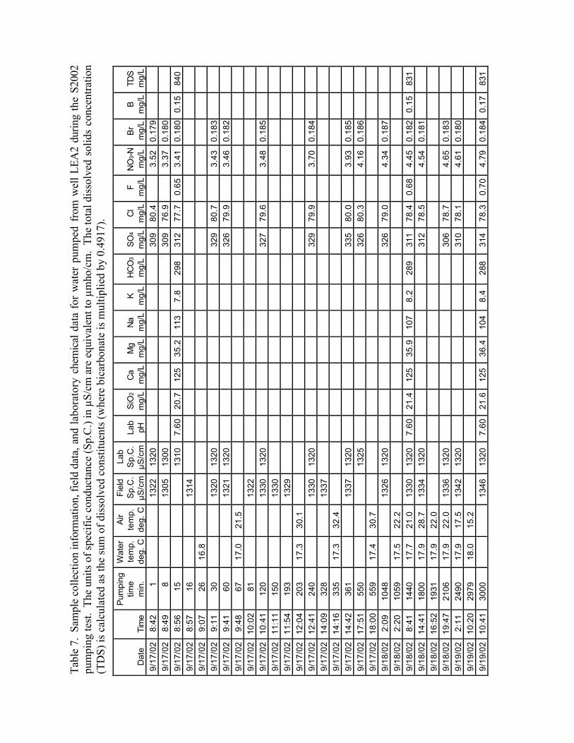
Polyethylene bottles were filled with water samples and placed in a cooler with ice fortransport to the analytical laboratories of the Kansas Geological Survey, where they weretransferred to a refrigerator until analysis. The concentrations of silica, cations, and boron weredetermined using inductively-coupled plasma spectrophotometry. Alkalinity was measured byautomated titrimetry and converted to bicarbonate content. Sulfate, chloride, nitrate, and bromideconcentrations were determined using colorimetric or ultraviolet spectrophotometry onautomated flow-injection or segmented-flow instruments. The chemical data for the watersamples for the pumping tests and associated observation wells are listed in Tables 7-9. Water-quality data obtained from sampling of selected observation wells for studies of stream-aquiferinteractions and phreatophyte water consumption at the O’Rourke Bridge site were used ininterpretation of the data from both pumping tests.
Results and Discussion
September 2002 (S2002) pumping test
The temperature of the water pumped from well LEA2 increased 0.5 °C during the first200 minutes of the pumping test and then rose slowly another 0.7 °C during the rest of the test(Table 7, Figure 36). Except for a small decrease during the first 15 minutes of pumping, thespecific conductance remained constant during the test. Sulfate and chloride concentrationsvaried by 17 mg/L and 3.8 mg/L during the first hour of pumping, increased by a small amountduring the next 10 hours, decreased slowly during the next 15 hours, and became relativelyconstant the rest of the test (Table 7, Figure 36). The estimated analytical precision of
Tab
le 7
. Sa
mpl
e co
llect
ion
info
rmat
ion,
fie
ld d
ata,
and
lab
orat
ory
chem
ical
dat
a fo
r w
ater
pum
ped
from
wel
l L
EA
2 du
ring
the
S20
02pu
mpi
ng te
st.
The
uni
ts o
f sp
ecif
ic c
ondu
ctan
ce (
Sp.C
.) in
µS/
cm a
re e
quiv
alen
t to µ
mho
/cm
. T
he to
tal d
isso
lved
sol
ids
conc
entr
atio
n(T
DS)
is c
alcu
late
d as
the
sum
of
diss
olve
d co
nstit
uent
s (w
here
bic
arbo
nate
is m
ultip
lied
by 0
.491
7).
Dat
eT
ime
Pum
ping
time
min
.
Wat
erte
mp
.de
g. C
Air
tem
p.
deg.
C
Fie
ldS
p.C
.µ
S/c
m
Lab
Sp
.C.
µS
/cm
Lab
pHS
iO2
mg/
LC
am
g/L
Mg
mg/
LN
am
g/L
Km
g/L
HC
O3
mg/
LS
O4
mg/
LC
lm
g/L
Fm
g/L
NO
3-N
mg/
LB
rm
g/L
Bm
g/L
TDS
mg/
L
9/1
7/0
28
:42
113
2213
2030
98
0.4
3.5
20
.17
9
9/1
7/0
28
:49
813
0513
0030
97
6.9
3.3
70
.18
0
9/1
7/0
28
:56
1513
107
.60
20
.712
53
5.2
113
7.8
298
312
77
.70
.65
3.4
10
.18
00
.15
840
9/1
7/0
28
:57
1613
14
9/1
7/0
29
:07
261
6.8
9/1
7/0
29
:11
3013
2013
2032
98
0.7
3.4
30
.18
3
9/1
7/0
29
:41
6013
2113
2032
67
9.9
3.4
60
.18
2
9/1
7/0
29
:48
671
7.0
21
.5
9/1
7/0
21
0:0
281
1322
9/1
7/0
21
0:4
112
013
3013
2032
77
9.6
3.4
80
.18
5
9/1
7/0
21
1:1
115
013
30
9/1
7/0
21
1:5
419
313
29
9/1
7/0
21
2:0
420
31
7.3
30
.1
9/1
7/0
21
2:4
124
013
3013
2032
97
9.9
3.7
00
.18
4
9/1
7/0
21
4:0
932
813
37
9/1
7/0
21
4:1
633
51
7.3
32
.4
9/1
7/0
21
4:4
236
113
3713
2033
58
0.0
3.9
30
.18
5
9/1
7/0
21
7:5
155
013
2532
68
0.3
4.1
60
.18
6
9/1
7/0
21
8:0
055
91
7.4
30
.7
9/1
8/0
22
:09
1048
1326
1320
326
79
.04
.34
0.1
87
9/1
8/0
22
:20
1059
17
.52
2.2
9/1
8/0
28
:41
1440
17
.72
1.0
1330
1320
7.6
02
1.4
125
35
.910
78
.228
931
17
8.4
0.6
84
.45
0.1
82
0.1
583
1
9/1
8/0
21
4:4
118
001
7.9
28
.713
3413
2031
27
8.5
4.5
40
.18
1
9/1
8/0
21
6:5
219
311
7.9
22
.0
9/1
8/0
21
9:4
721
061
7.9
22
.013
3613
2030
67
8.7
4.6
50
.18
3
9/1
9/0
22
:11
2490
17
.91
7.5
1342
1320
310
78
.14
.61
0.1
80
9/1
9/0
21
0:2
029
791
8.0
15
.2
9/1
9/0
21
0:4
130
0013
4613
207
.60
21
.612
53
6.4
104
8.4
288
314
78
.30
.70
4.7
90
.18
40
.17
831

Tab
le 8
. Sa
mpl
e co
llect
ion
info
rmat
ion,
fie
ld d
ata,
and
lab
orat
ory
chem
ical
dat
a fo
r w
ater
pum
ped
from
wel
l IW
dur
ing
the
O20
03pu
mpi
ng te
st.
See
Tab
le 7
abo
ve f
or e
xpla
natio
n of
Sp.
C. a
nd T
DS.
Sam
ple
da
teS
ampl
etim
e
Pum
ping
time
min
.
Fie
ldS
p.C
.µ
S/c
m
Lab
Sp
.C.
µS
/cm
Lab
pHS
iO2
mg/
LC
am
g/L
Mg
mg/
LN
am
g/L
Km
g/L
HC
O3
mg/
LS
O4
mg/
LC
lm
g/L
Fm
g/L
NO
3-N
mg/
LB
rm
g/L
Bm
g/L
TDS
mg/
L
10
/20
/03
11
:30
-35
1360
1335
7.4
51
8.6
157
31
.710
05
.427
339
55
7.4
0.5
32
.15
0.2
32
0.1
29
911
10
/20
/03
12
:10
517
0016
707
.40
19
.418
63
6.9
154
6.3
295
545
81
.30
.65
2.5
30
.27
20
.17
611
87
10
/20
/03
12
:20
1517
0416
9053
98
1.8
2.3
9
10
/20
/03
12
:50
4516
3716
107
.40
19
.718
43
6.6
142
6.0
291
530
74
.00
.58
2.1
90
.26
60
.15
011
47
10
/20
/03
13
:15
7015
6515
507
.40
19
.417
93
5.6
130
5.7
287
513
71
.00
.54
2.1
00
.25
60
.13
511
06
10
/20
/03
14
:30
145
1472
1450
464
64
.01
.90
10
/20
/03
16
:53
288
1377
1360
7.4
01
8.4
159
31
.610
15
.227
542
65
8.9
0.5
11
.94
0.2
35
0.1
11
946
10
/21
/03
8:3
412
2913
8313
607
.60
18
.716
33
2.7
103
4.8
275
420
58
.60
.50
2.0
30
.23
30
.10
494
7
10
/21
/03
19
:07
1862
1360
427
58
.52
.12
10
/22
/03
9:4
927
4413
757
.45
19
.016
43
2.5
104
5.2
276
426
59
.60
.49
2.1
00
.23
90
.10
895
7
10
/22
/03
18
:55
3290
1375
427
58
.92
.10
10
/23
/03
8:5
141
2613
8042
85
9.2
2.1
0
10
/23
/03
18
:40
4715
1385
430
59
.52
.17
10
/24
/03
10
:18
5653
1390
7.4
01
9.0
165
32
.710
55
.227
844
45
9.2
0.4
92
.17
0.2
43
0.1
22
978
Tab
le 9
. Sa
mpl
e co
llect
ion
info
rmat
ion,
fie
ld d
ata,
and
labo
rato
ry c
hem
ical
dat
a fo
r w
ater
pum
ped
from
wel
ls u
sed
as o
bser
vatio
nw
ells
in th
e O
2003
pum
ping
test
. Se
e Fi
gure
1b
for
an a
real
vie
w o
f ob
serv
atio
n w
ell
netw
ork.
See
Tab
le 7
abo
ve f
or e
xpla
natio
n of
Sp.C
. and
TD
S. S
ee T
able
10
for
wel
l dep
th a
nd s
cree
ned
inte
rval
info
rmat
ion.
Wel
l No.
Sam
ple
da
teS
ampl
etim
e
Fie
ldS
p.C
.µ
S/c
m
Lab
Sp
.C.
µS
/cm
Lab
pHS
iO2
mg/
LC
am
g/L
Mg
mg/
LN
am
g/L
Km
g/L
HC
O3
mg/
LS
O4
mg/
LC
lm
g/L
Fm
g/L
NO
3-N
mg/
LB
rm
g/L
Bm
g/L
TDS
mg/
L
PT
1a1
/24
/04
11
:54
1475
1460
473
56
.81
.2
PT
1a1
/24
/04
12
:13
1466
1450
7.8
01
9.1
180
36
.19
3.9
4.3
267
462
56
.00
.48
1.2
0.2
63
0.1
03
983
PT
1b1
/24
/04
12
:57
1874
1850
609
95
.82
.1
PT
1b1
/24
/04
13
:12
1874
1850
8.1
01
9.4
193
40
.318
17
.230
260
59
5.1
0.7
12
.20
.28
70
.22
912
90
PT
5a1
/24
/04
10
:00
1159
1140
249
59
.13
.6
PT
5a1
/24
/04
10
:15
1158
1140
8.0
01
7.5
122
24
.68
8.0
4.9
274
266
59
.10
.52
3.6
0.1
72
0.1
07
717
PT
5b1
/24
/04
10
:57
2020
1950
668
101
1.9

43
PT
5b1
/24
/04
11
:02
2020
1960
8.0
51
8.8
214
42
.419
27
.232
366
810
00
.74
1.9
0.3
13
0.2
27
1402

43
Table 10. Specific conductance of ground water in the screened interval of the observation wellsinstalled for the O2003 pumping test.
Measured or estimated mean Sp.C., µS/cm,In screened interval
WellWell depth,
ft bls*Screened
interval, ft bls
Field value fromconductance profile
11/12/2003
Lab value forpumped sample
1/24/04
Field value fromconductance profile
2/25/04
Alluvial aquifer
PT1b 28.1 12.9-22.7 1801 1850 1799
PT2 24.4 14.1-24.0 1759
PT4b 25.1 14.9-24.7 958
PT5b 29.8 19.6-29.4 1923 1960 2080
High Plains aquifer
PT1a 67.1 61.9-66.7 1595 1450
PT3 67.1 61.9-66.7 2130
PT4a 67.1 61.9-66.7 2130
PT5a 66.3 61.1-65.9 1140
* Feet below land surface
the sulfate and chloride determinations is about 1% of the sulfate values (~3 mg/L) andapproximately 0.5% for the chloride values (~0.4 mg/L). Thus, the very small changes inconcentration during the second half of the test could be largely due to analytical error. After avery small decrease during the 8 minutes of pumping, the nitrate concentration increased duringthe rest of the test (Table 7, Figure 36). The estimated precision in the nitrate concentration isabout 0.05 mg/L. Therefore, the greater rate of increase in nitrate content during the first 10hours of pumping compared to the rest of the test is analytically verifiable.
Temperature measured in and chemical data for water samples collected from monitoringwells at the O’Rourke Bridge site within a year following the S2002 pumping test help ininterpreting the changes observed during that test. The data indicate that the primary cause forthe temperature and chemical changes is water drawn in laterally from under the river channel tothe west of well LEA2 and not water flowing vertically from below the screened interval of thewell. The temperature and water chemistry of the ground waters at the location of well LEA2changes both vertically within the entire alluvial aquifer and laterally within the aquifer towardsthe river. As the well was pumped during the test, the lateral radius within which ground waterwas captured in the most permeable strata grew to include the area near and just under the riverchannel. A small clay layer at 17 ft bls (Figure 6) retarded the vertical movement of ground waterfrom below the screen interval of LEA2 (11.4-16.1 ft bls).
A temperature profile measured at one-foot intervals in well LEA2 a year after (9/18/03)the S2002 test showed a temperature decrease with depth (from 20.0 to 18.7 °C) for the depthinterval 8-17 ft bls. The decreasing temperature with depth represented the warming of theshallower water by summer temperatures. Therefore, the 1.2 °C warming of the water during thepumping test (Figure 36) cannot be explained by upconing of deeper aquifer water.

44
16.8
17.2
17.6
18.0T
em
pe
ratu
re, d
eg
. C
300
320
340
Su
lfate
, mg
/L
77
78
79
80
81
Chl
ori
de
, mg
/ L
0 500 1000 1500 2000 2500 3000
M inutes from start o f pumping tes t
3.2
3.6
4.0
4.4
4.8
Nitr
ate
-N,
mg
/ L

45
Figure 36. Change in temperature and sulfate, chloride, and nitrate concentrations of thedischarged water during the S2002 pumping test.
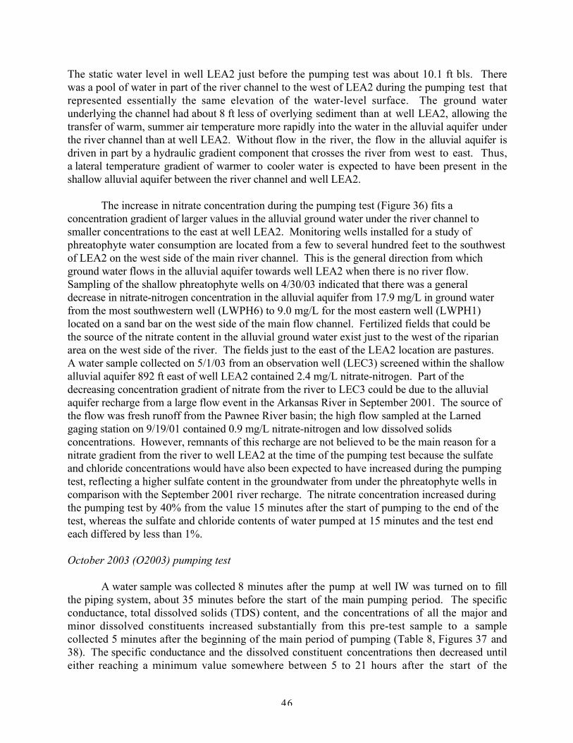
46
The static water level in well LEA2 just before the pumping test was about 10.1 ft bls. Therewas a pool of water in part of the river channel to the west of LEA2 during the pumping test thatrepresented essentially the same elevation of the water-level surface. The ground waterunderlying the channel had about 8 ft less of overlying sediment than at well LEA2, allowing thetransfer of warm, summer air temperature more rapidly into the water in the alluvial aquifer underthe river channel than at well LEA2. Without flow in the river, the flow in the alluvial aquifer isdriven in part by a hydraulic gradient component that crosses the river from west to east. Thus,a lateral temperature gradient of warmer to cooler water is expected to have been present in theshallow alluvial aquifer between the river channel and well LEA2.
The increase in nitrate concentration during the pumping test (Figure 36) fits aconcentration gradient of larger values in the alluvial ground water under the river channel tosmaller concentrations to the east at well LEA2. Monitoring wells installed for a study ofphreatophyte water consumption are located from a few to several hundred feet to the southwestof LEA2 on the west side of the main river channel. This is the general direction from whichground water flows in the alluvial aquifer towards well LEA2 when there is no river flow. Sampling of the shallow phreatophyte wells on 4/30/03 indicated that there was a generaldecrease in nitrate-nitrogen concentration in the alluvial aquifer from 17.9 mg/L in ground waterfrom the most southwestern well (LWPH6) to 9.0 mg/L for the most eastern well (LWPH1)located on a sand bar on the west side of the main flow channel. Fertilized fields that could bethe source of the nitrate content in the alluvial ground water exist just to the west of the riparianarea on the west side of the river. The fields just to the east of the LEA2 location are pastures. A water sample collected on 5/1/03 from an observation well (LEC3) screened within the shallowalluvial aquifer 892 ft east of well LEA2 contained 2.4 mg/L nitrate-nitrogen. Part of thedecreasing concentration gradient of nitrate from the river to LEC3 could be due to the alluvialaquifer recharge from a large flow event in the Arkansas River in September 2001. The source ofthe flow was fresh runoff from the Pawnee River basin; the high flow sampled at the Larnedgaging station on 9/19/01 contained 0.9 mg/L nitrate-nitrogen and low dissolved solidsconcentrations. However, remnants of this recharge are not believed to be the main reason for anitrate gradient from the river to well LEA2 at the time of the pumping test because the sulfateand chloride concentrations would have also been expected to have increased during the pumpingtest, reflecting a higher sulfate content in the groundwater from under the phreatophyte wells incomparison with the September 2001 river recharge. The nitrate concentration increased duringthe pumping test by 40% from the value 15 minutes after the start of pumping to the end of thetest, whereas the sulfate and chloride contents of water pumped at 15 minutes and the test endeach differed by less than 1%.
October 2003 (O2003) pumping test
A water sample was collected 8 minutes after the pump at well IW was turned on to fillthe piping system, about 35 minutes before the start of the main pumping period. The specificconductance, total dissolved solids (TDS) content, and the concentrations of all the major andminor dissolved constituents increased substantially from this pre-test sample to a samplecollected 5 minutes after the beginning of the main period of pumping (Table 8, Figures 37 and38). The specific conductance and the dissolved constituent concentrations then decreased untileither reaching a minimum value somewhere between 5 to 21 hours after the start of the
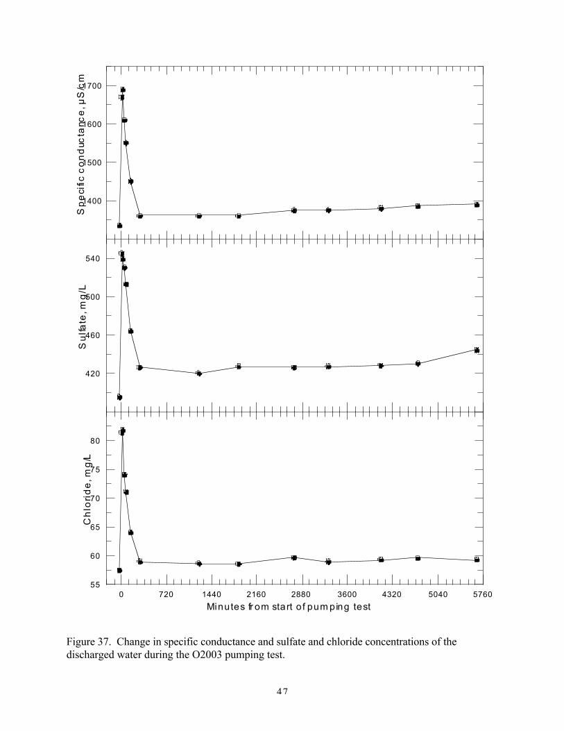
47
Figure 37. Change in specific conductance and sulfate and chloride concentrations of thedischarged water during the O2003 pumping test.
1400
1500
1600
1700S
pe
cific
co
nd
ucta
n ce
, µS
/cm
420
460
500
540
Su
lfate
, mg
/L
0 720 1440 2160 2880 3600 4320 5040 5760
Minutes fr om start o f pum ping test
55
60
65
70
75
80
Ch
lori
de
, mg
/ L

48
Figure 38. Change in calcium, sodium, and nitrate concentrations of the discharged water duringthe O2003 pumping test.
160
170
180
190C
alc
ium
, mg
/L
100
110
120
130
140
150
So
diu
m,
mg
/L
0 720 1440 2160 2880 3600 4320 5040 5760
M inutes from start o f pumping test
1.8
2.0
2.2
2.4
Nitr
ate
-N, m
g/L

49
the main period of pumping or stabilizing during the rest of the test (Table 8, Figures 37 and 38).Except for sulfate, the minimum values of all major constituent concentrations and the specificconductance in the samples collected from 288 to 1229 minutes (4.8-20.5 hours) after the start ofthe main pumping period differed from the pre-test sample by only about 2% or less. Theminimum values for the TDS and sulfate concentrations in the 4.8 to 20.5 hour samples wereapproximately 4% and 6% greater than in the pre-test sample, whereas the minimum value fornitrate was about 12% lower than in the pre-test sample. The minimum for nitrate was reachedafter 145 minutes (2.4 hours) of pumping. After a day of pumping, the specific conductance,TDS, and concentrations of nearly all dissolved constituents increased slightly until the end ofthe test. The values for specific conductance and the concentrations of TDS and all measureddissolved constituents except sulfate differed by less than 8% between the pre-test and test-endsamples. The sulfate content in the last sample was about 12% greater than in the pre-test water.
The chemical relationships for waters in the alluvial and High Plains aquifers and pastArkansas River flow in the study area provide insights into the origin of constituents and changesin the water pumped during the test. The arrows on the lines connecting the filled circles for theO2003 pumping test on Figures 39 and 40 indicate the progression of the chemical changes duringthe test period. Larger filled circles in the figures represent chemical data for samples from theHigh Plains aquifer collected from two observation wells (PT1a and PT5a) in the nests installednearest well IW for the pumping test, and from observation wells LWC2 and LWPH4c installedfor stream-aquifer and phreatophyte studies, respectively. Unfilled circles in Figures 39 and 40represent chemical data for samples from the alluvial aquifer collected from four observationwells (PT1b, PT5b, LWC1 and LWPH4b) next to the observation wells in the High Plainsaquifer. The thin lines connecting points for Arkansas River water collected either at Larned orthe Larned gaging station during the past decade enclose the ranges in dissolved constituentconcentrations for the river.
The points for well nests PT1 and PT5 on Figures 39 and 40 represent samples collectedfrom the wells three months after the O2003 pumping test. Table 10 compares the specificconductance of these samples with field values from conductance profiles measured in some ofthe wells before and after the sampling, along with profiles for other observation wells installedfor the O2003 test. The conductance profiles for the wells installed in the High Plains aquifer didnot reach the screened interval because the probe cable is only 50 ft long. In addition, surfacetension on the probe cable from the wet PVC surface in the small diameter (1.0-inch diameter)wells prevented the probe from sinking further than 44-46 ft below the top of the well casing. Even though the conductance profile did not reach the screened interval, the relatively constantconductance measured in the profile and the fact that the wells had been developed indicate thatthe water in the column was representative of water that had been produced from the aquifer. Table 10 indicates that the water in the High Plains aquifer at well PT1a was somewhat lesssaline three months after the pumping test in comparison with one month after the test. Theconductance of ground water in the alluvial aquifer at well PT1b remained relatively constantfrom one to 4 months after the pumping test, whereas the salinity of ground water at well PT5bincreased a small amount.
The specific conductance and concentration of TDS and nearly all dissolved constituentsin the samples collected just prior to and at the end of the pumping test were between the values
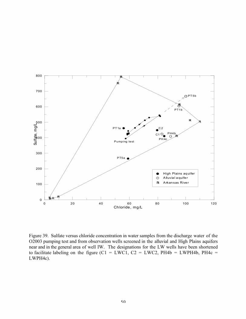
50
0 20 40 60 80 100 120Chloride, mg/L
0
100
200
300
400
500
600
700
800
Sulfa
te, m
g/L
PT 1a
PT1b
PT 5b
PT5a
PH4b
C 2
C1
PH 4cPumping test
High Plains aq uiferA lluvia l a quife r
A rkan sas Rive r
Figure 39. Sulfate versus chloride concentration in water samples from the discharge water of theO2003 pumping test and from observation wells screened in the alluvial and High Plains aquifersnear and in the general area of well IW. The designations for the LW wells have been shortenedto facilitate labeling on the figure (C1 = LWC1, C2 = LWC2, PH4b = LWPH4b, PH4c =LWPH4c).
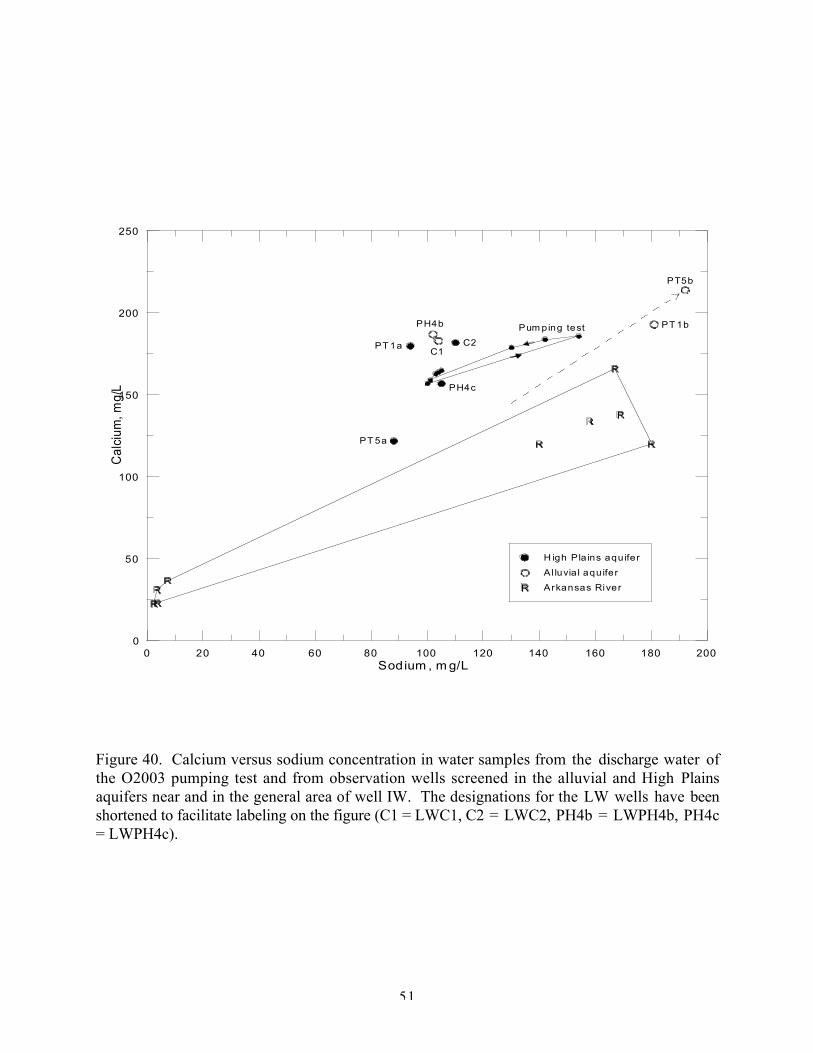
51
0 20 40 60 80 100 120 140 160 180 200Sodium , m g/L
0
50
100
150
200
250
Cal
cium
, mg/
L
PT 1a
PT 1b
PT5b
PT 5a
PH4b
C2C1
PH4c
Pum ping test
H igh Pla ins aquifer
Al luvia l aquifer
Arkansas River
Figure 40. Calcium versus sodium concentration in water samples from the discharge water ofthe O2003 pumping test and from observation wells screened in the alluvial and High Plainsaquifers near and in the general area of well IW. The designations for the LW wells have beenshortened to facilitate labeling on the figure (C1 = LWC1, C2 = LWC2, PH4b = LWPH4b, PH4c= LWPH4c).
52
for samples collected from observation wells PT1a and PT5a (Tables 8 and 9, Figures 39 and40). Thus, the average composition of the ground water in the High Plains aquifer surroundingwell IW, but at a distance outside the radius of the impact of gravel-pack flow from the well sincethe last period of irrigation pumping, was generally between the compositions at wells PT1a andPT5a. The concentrations of sulfate, chloride, calcium, and sodium were substantially greater inthe alluvial aquifer than in the pre-test sample from the irrigation well in the High Plains aquiferin contrast to generally similar concentrations for well sites LWC and LWPH4 (except forcalcium at site LWPH4) (Figures 39 and 40).
The points for samples from wells PT1b and PT5b on Figure 39 either lie outside or atthe edge of the enclosed range for points representing Arkansas River waters, whereas the pointsfor the other well samples lie within the river chemistry boundaries. Evapotranspirationconsumption of irrigation water withdrawn from the alluvial and High Plains aquifershydraulically up-gradient from the site, followed by infiltration of the more concentrated water(containing the residual dissolved solids) to the water table and flow to well IW is believed to bethe cause for the higher sulfate and chloride concentrations. The dashed line pointing to thesymbol for well PT5b represents the direction in which the chemistry would change ifconservative (without reaction) concentration of sulfate and chloride occurred due toconsumption of water leaving dissolved constituents in the smaller volume of residual water. Figure 40 shows that the points for all the well waters lie above (at higher calcium concentration)the boundaries for the range in river composition. The source of much of the additional calciumcould be weathering and dissolution of minerals in the aquifer sediments, particularly calcite. Inaddition, the higher calcium content could partially reflect the composition of ground waterflowing into the alluvium and the High Plains aquifer from the Cretaceous bedrock to the west. Except for waters from wells PT1b and PT5b, the sodium concentration of the ground watersrepresented in Figure 40 lie within the range for the river water. The evapotranspirationconcentration mechanism also fits as an explanation for the higher calcium and sodiumconcentrations in the water from wells PT1b and PT5b in comparison with the other groundwaters in the area. The dashed line pointing to the symbol for well PT5b in Figure 40 representsthe evapotranspiration concentration change in a similar manner as it does in Figure 39.
The spike in the constituent concentrations after the start of the pumping test (Figures 37and 38) is consistent with the withdrawal of High Plains aquifer water in which was mixed somealluvial aquifer water. The water-level declines described earlier in this report for the pumpingtest indicate that well IW is screened in the High Plains aquifer. The water-quality data alsosupport this because, if the screened interval of the well included part of the alluvial aquifer, thelarge concentration spike at the start of the pumping test would not be expected because therewould be a consistent mix of alluvial and High Plains aquifer waters. Leakage of alluvial aquiferwater through the low-permeability confining layer to the underlying High Plains aquifer, bothduring periods of pumping and no pumping, is expected to occur across the study area andtherefore would not be a cause for the substantial changes in water quality in the first few hoursof the test. The concentration spike can best be explained by the movement of alluvial aquiferwater down the gravel pack in the annular space between the casing and borehole of well IW. There was a static head gradient of approximately 1.6-1.9 ft between the alluvial aquifer and theHigh Plains aquifer based on water-level measurements obtained during three different dayswithin the week prior to the pumping test from the pairs of observation wells at sites PT1 and

53
PT5. The pre-test sample (-35 min in Table 8) represented water in the pipe extending 1584 ftfrom well IW to the center pivot that remained from the previous period the well was used forirrigation, and that was pushed to the center pivot during the short pre-test pumping. The wellwas last pumped for irrigation 12 days prior to the pumping test. Between that time and thestart of the pumping test, water flowed slowly down the gravel pack from the alluvial aquiferinto the upper portions of the High Plains aquifer. Whittemore and Butler described themechanism of gravel pack flow associated with large-diameter wells as being potentiallyimportant for the movement of shallow, saline water into the High Plains aquifer along the upperArkansas River corridor (Whittemore and Butler, 1997).
The mixing of different waters on Figures 39 and 40 can be represented by straight lines.Extension of the straight line, which indicates the substantial increase in dissolved constituentconcentrations from the pre-test to the 5-minute pumping sample in Figures 39 and 40, to greaterconcentrations indicates that water similar to that in the alluvial aquifer in the area of theirrigation well (as represented by samples from observation wells PT1b and PT5b) is the mostlikely source of the concentration jump. This relationship supports the mixing of alluvial aquiferwater with High Plains aquifer water through flow down the gravel pack of well IW. The alluvialaquifer water that reached the High Plains aquifer between the last period of irrigation pumpingand the O2003 pumping test is expected to have been concentrated in the area immediatelyaround and down hydraulic gradient from the screen in well IW, and in the upper part of the HighPlains aquifer. During the first five hours of pumping, most of the alluvial aquifer water thatentered the High Plains aquifer via the gravel pack between the last period of irrigation pumpingand the O2003 test was removed. The last time well IW was pumped was from 9:15 to 14:00 onOctober 8, 2003; the well was shut off when rain began that totaled 0.92 inch on that afternoon. The period of pumping, 4.75 hrs (285 min) was very close to the pumping-test time at which theconcentration spike in Figures 37 and 38 ended (4.8 hrs or 288 min).
The gravel-pack flow during the period of no pumping between October 8 and October 20can be estimated by determining the volume of alluvial aquifer water removed from the HighPlains aquifer during the first few hours of the pumping test as indicated by the concentrationpeaks in Figures 37 and 38. Although gravel-pack flow prior to the October 8 pumping alsoentered the High Plains aquifer, the concentration spike during the first part of the pumping testis assumed to represent mainly the new flow into the aquifer since the end of the last pumpingperiod. The flow rate of ground water in the High Plains aquifer is expected to be small enoughthat the pumping test was able to capture most of the plume of the gravel-pack flow since thelast period of pumping. For example, if the flow rate were as high as a foot per day, the plumefrom the new gravel-pack flow would have traveled 12 feet since the last pumping. The volumeof water pumped during the pumping test would be equivalent to capturing ground water withina cylinder of radius 137 ft in the High Plains aquifer, assuming an average pumping rate of 358gpm, homogenous flow, an average aquifer thickness of 18.4 ft, and an effective porosity of 25%from which water was withdrawn.
The first step in the estimation of gravel-pack flow from October 8 to 20 is computationof the percentage of water pumped with an alluvial aquifer composition at each sampling time inTable 8 during the concentration spike shown in Figures 37 and 38. The mixing equation

54
Cmix = vC1 + (1-v)C2
can be used to calculate the concentration of a dissolved constituent C in a mixture of two end-member waters, where v is the volume fraction of the first end member water. For thiscalculation, the chemistry of the pre-test sample is used for C1 and is assumed to representground-water in the High Plains aquifer pumped at the end of the last irrigation withdrawal. Itscomposition would include long-term, past gravel-pack flow and leakage through the low-permeability layer at the end of that pumping. The composition of C2 could be represented as anaverage of the alluvial aquifer water at sites PT1 and PT5. These wells were screened in thelower part of the alluvial aquifer (Table 10) above the low-permeability layer that separates itfrom the underlying High Plains aquifer. The variable Cmix is the concentration measured in thewater for each sampling time.
The best constituents to use for the calculation are those that do not differ substantiallybetween wells PT1a and PT5a in the High Plains aquifer, but differ substantially between theHigh Plains aquifer and the alluvial aquifer (wells PT1b and PT5b). Constituents such ascalcium, magnesium, and sulfate differ enough between wells PT1a and PT5a that changes duringthe pumping test could be partly controlled by chemical heterogeneity in the High Plains aquifer. For example, there is a gradient of increasing specific conductance (and thus dissolvedconstituent concentrations) from well PT5a toward the Arkansas River channel as indicated bythe values for wells PT1a, PT3, and PT4a (Table 10). Constituents such as sodium and chloridehave relatively similar concentrations in samples from the High Plains aquifer (PT1a and PT5a),which differ substantially from concentrations in the alluvial aquifer (PT1b and PT5b). Thechloride concentration in the samples collected from PT1a and PT5a differed by only 3.1 mg/Land averaged 57.6 mg/L (Table 9), a value essentially the same as the 57.4 mg/L in the pre-testsample (Table 8). The sodium content of the PT1a and PT5a samples differed by 5.9 mg/L andaveraged 91.0 mg/L, which was only 9 mg/L lower than the pre-test concentration of 100 mg/L.
The values used for C1 for chloride and sodium were the pre-test concentrations of 57.4mg/L and 100 mg/L, respectively. The values used for C2 for chloride and sodium in the alluvialaquifer were 97.6 mg/L and 186 mg/L, respectively, the averages for samples from wells PT1band PT5b. The volume percentages of alluvial aquifer water in Cmix obtained from thecomputation for the samples collected up to 288 minutes after the start of the main pumpingperiod using chloride and sodium concentrations were multiplied by the pumping rate at eachsampling time to obtain a flow rate for alluvial aquifer water. The flow rate for alluvial aquiferwater calculated from the mixing-curve equation for the 288 min sample was assumed torepresent the combined leakage through the low-permeability layer and the gravel-pack flowoccurring during the pumping test, and was subtracted from all the calculated flow rates for theprevious sampling times. The area was calculated under the curves for plots of the flow ratecontribution derived from the alluvial aquifer due to prior gravel-pack flow versus pumping time(Figure 41). This area (in gal) was divided by the time (17,165 min) between the end of the lastperiod of irrigation pumping and the start of the O2003 pumping test to obtain the gravel-packflow rate. The plot based on chloride concentrations is generally better than that based onsodium because it includes more sample points. The results, 1.4 gpm and 1.7 gpm based on thechloride and sodium data, respectively, suggest that the gravel-pack flow during period of no

55
Figure 41. Change in flow rate attributed to alluvial aquifer water mixed with High Plains aquiferwater during the initial concentration spike of the O2003 pumping test.
0
50
100
150
200
250F
low
rate
att
ri but
e d t o
all u
via l
aq u
i fer
w
ate
r fro
m p
r io r
gr a
v el -
pac k
f lo w
, gp m
0 100 200 300Time since s tart o f pumping, minutes
0
50
100
150
200
250
Flo
w r
ate
att r
ibut
e d t
o a l
luvi
al a
q uif e
r w
ate
r f r
om p
rio r
gra
v el- p
a ck
flo
w,
gpm
Computation bas ed on chloride conc entration
Computation bas ed on sodium concentr ation

56
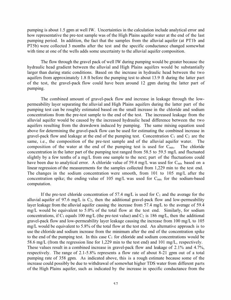
57
pumping is about 1.5 gpm at well IW. Uncertainties in the calculation include analytical error andhow representative the pre-test sample was of the High Plains aquifer water at the end of the lastpumping period. In addition, the fact that the samples from the alluvial aquifer (at PT1b andPT5b) were collected 3 months after the test and the specific conductance changed somewhatwith time at one of the wells adds some uncertainty to the alluvial aquifer composition.
The flow through the gravel pack of well IW during pumping would be greater because thehydraulic head gradient between the alluvial and High Plains aquifers would be substantiallylarger than during static conditions. Based on the increase in hydraulic head between the twoaquifers from approximately 1.8 ft before the pumping test to about 13.9 ft during the latter partof the test, the gravel-pack flow could have been around 12 gpm during the latter part ofpumping.
The combined amount of gravel-pack flow and increase in leakage through the low-permeability layer separating the alluvial and High Plains aquifers during the latter part of thepumping test can be roughly estimated based on the small increase in the chloride and sodiumconcentrations from the pre-test sample to the end of the test. The increased leakage from thealluvial aquifer would be caused by the increased hydraulic head difference between the twoaquifers resulting from the drawdown induced by pumping. The same mixing equation usedabove for determining the gravel-pack flow can be used for estimating the combined increase ingravel-pack flow and leakage at the end of the pumping test. Concentration C1 and C2 are thesame, i.e., the composition of the pre-test sample and of the alluvial aquifer water. Thecomposition of the water at the end of the pumping test is used for Cmix. The chlorideconcentration in the latter part of the pumping test ranged from 58.5 to 59.5 mg/L and fluctuatedslightly by a few tenths of a mg/L from one sample to the next; part of the fluctuations couldhave been due to analytical error. A chloride value of 59.4 mg/L was used for Cmix based on alinear regression of the measurements for the samples collected from 1,229 min to the test end. The changes in the sodium concentration were smooth, from 101 to 105 mg/L after theconcentration spike; the ending value of 105 mg/L was used for Cmix for the sodium-basedcomputation.
If the pre-test chloride concentration of 57.4 mg/L is used for C1 and the average for thealluvial aquifer of 97.6 mg/L is C2, then the additional gravel-pack flow and low-permeabilitylayer leakage from the alluvial aquifer causing the increase from 57.4 mg/L to the average of 59.4mg/L would be equivalent to 5.0% of the total flow at the test end. Similarly, for sodiumconcentrations, if C1 equals 100 mg/L (the pre-test value) and C2 is 186 mg/L, then the additionalgravel-pack flow and low-permeability layer leakage causing the increase from 100 mg/L to 105mg/L would be equivalent to 5.8% of the total flow at the test end. An alternative approach is touse the chloride and sodium increase from the minimum after the end of the concentration spiketo the end of the pumping test. In this case C1 for chloride and sodium concentrations would be58.6 mg/L (from the regression line for 1,229 min to the test end) and 101 mg/L, respectively. These values result in a combined increase in gravel-pack flow and leakage of 2.1% and 4.7%,respectively. The range of 2.1-5.8% represents a flow rate of about 8-21 gpm out of a totalpumping rate of 358 gpm. As indicated above, this is a rough estimate because some of theincrease could possibly be due to withdrawal of somewhat higher TDS water from different partsof the High Plains aquifer, such as indicated by the increase in specific conductance from the

58
vicinity of well IW to the river. In addition to the uncertainties described for the gravel-packflow estimate above, there is a significant lag time for the alluvial aquifer water to move throughthe low-permeability layer, so the leakage entering the top of the High Plains aquifer during thepumping test represents older ground water from the alluvial aquifer.
Summary
The water-quality data indicate that water pumped during the S2002 pumping test in theArkansas River alluvial aquifer included some ground water from under the main river channel. Thus, if the river were flowing, river water would also have been expected to be drawn into thealluvial aquifer.
The effect of subregional pumping on the High Plains aquifer produces a lower hydraulichead in the High Plains aquifer than in the overlying alluvial aquifer. This results in downwardflow of alluvial aquifer water through the low-permeability layer separating the aquifers. Depending on the age of the irrigation well, it can also result in downward flow through the gravelpack of the irrigation well. The water-quality effect of this flow was observed during the O2003pumping test in the High Plains aquifer. When the river is flowing, the downward flow of waterfrom the alluvium into the High Plains aquifer either decreases the discharge of alluvial groundwater into the river or, if the river stage is greater than the water level in the aquifer, increases thedischarge of river water into the alluvial aquifer. When the river is not flowing, this downwardflow of water causes a water-level decline under the river channel. The induced flow of waterfrom the alluvial aquifer to the High Plains aquifer also results in the downward migration ofshallow water with more salinity and containing other constituents such as nitrate from surfacesources. Chemical data collected as part of other projects in the area of the O’Rourke Bridge sitesupports this conceptual model. As indicated in the sections on the pumping test analysis, thelag time required for pumping in the alluvial aquifer to significantly affect river flow is expectedto be substantially less than that required for pumping in the High Plains aquifer in the rivervalley, given equal distances of the pumping wells from the river.

59
ACKNOWLEDGEMENTS
This study was partially supported by a contract with the Kansas Department ofAgriculture, Division of Water Resources (DWR). The agreement of Lee Borck of Ward FeedYard to allow the use of well IW for the O2003 pumping test is greatly appreciated. RexBuchanan and Brownie Wilson of the KGS, and David Zook, Mark Billinger, Nick Campas, andMindy Sleck of the DWR assisted in the O2003 pumping test by measuring water levels duringthe test. Jeff Lanterman and David Zook of the DWR measured the pumping rate during theO2003 test using the Panametrics ultrasonic flowmeter. Larry Hathaway and Mike Magnuson ofthe KGS analyzed the water samples. Tina Alder of the DWR reviewed the report and providedcomments for its improvement.

60
REFERENCES
Butler, J.J., Jr. 1988. Pumping tests in nonuniform aquifers - the radially symmetric case. Journalof Hydrology, v. 101, no. 1/4, pp. 15-30.
Butler, J.J., Jr. 1998. The Design, Performance, and Analysis of Slug Tests. Boca Raton, LewisPublishers.
Butler, J.J., Jr., Healey, J.M., Zheng, L., McCall, W., and M.K. Schulmeister, 1999,Hydrostratigraphic characterization of unconsolidated alluvium with direct-push sensortechnology, Kansas Geological Survey Open-File Report 99-40.
Butler, J.J., Jr., Loheide, S.P., II, Kluitenberg, G.J., Bayless, K., Whittemore, D.O., Zhan, X.,C.E. Martin. 2004. Groundwater consumption by phreatophytes in a mid-continentstream-aquifer system (abstract), Eos, v. 85, no. 17, Jt. Assem. Suppl., p. JA237.
Christy, C.D., Christy, T.M., and V. Wittig, 1994, A percussion probing tool for the directsensing of soil conductivity, In: Proc. of the 8th National Outdoor Action Conf., NGWA,pp. 381-394.
HydroSOLVE, Inc. 2001. AQTESOLV for Windows User’s Guide.
Kruseman, G.P. and N.A. de Ridder. 1990. Analysis and Evaluation of Pumping Test Data - ILRIpublication 47. ILRI, The Netherlands. 377 pp.
Moench, A.F., 1985. Transient flow to a large-diameter well in an aquifer with storativesemiconfining layers, Water Resources Research, vol. 21, no. 8, pp. 1121-1131.
Moench, A.F., 1997. Flow to a well of finite diameter in a homogeneous, anisotropic water tableaquifer, Water Resources Research, vol. 33, no. 6, pp. 1397-1407.
Sánchez-Vila, X., Meier, P.M., and J. Carrera. 1999. Pumping tests in heterogeneous aquifers: Ananalytical study of what can be obtained from their interpretation using Jacob’s method,Water Resources Research, vol. 35, no. 4, pp. 943-952.
Schulmeister, M.K., Butler, J.J., Jr., Healey, J.M., Zheng, L., Wysocki, D.A., and G.W. McCall,2003, Direct-push electrical conductivity logging for high-resolution hydrostratigraphiccharacterization, Ground Water Monitoring and Remediation, vol. 23, no. 5, pp. 52-62.
Whittemore, D.O., and J.J. Butler, Jr., 1997, Invasion of saline water along the Arkansas River: Hydrogram, Kansas Water Office, Topeka, KS, Spring issue, p. 11.