Kappa-tau type PI tuning rules for specified robust levels

Juan J. Gude1, 2 and Evaristo Kahoraho1

1 Department of Industrial Technologies University of Deusto

Avda. de las Universidades, 24 48007 Bilbao, Spain

2 DeustoTech Energy University of Deusto

Avda. de las Universidades, 24 48007 Bilbao, Spain

e-mail: jgude@deusto.es

Abstract: New tuning rules for 2-DoF PI controllers in the spirit of the kappa-tau ones are addressed in this paper. In particular, tuning rules have been devised in order to minimize the integrated absolute error with a constraint on the maximum sensitivity MS. Different tuning rules have been obtained for a batch of plants and for several robustness levels in terms of MS. The setpoint weight is also exploited to improve the setpoint following performance because the PI controller is tuned by optimizing the load disturbance rejection performance. In particular, explicit tuning rules are given in order to select the optimal setpoint weight to minimize the integrated absolute error. Simulation results demonstrate the effectiveness of these methodologies. Some comments relating to industrial practice are offered in this context. Keywords: Control design, tuning methods, PID control, optimization, process control.

1. INTRODUCTION

In spite of all the advances in process control over the past several decades, the proportional integral (PI) and the proportional integral derivative (PID) controller remains to be certainly the most extensive option that can be found on industrial control applications, see (Åström and Hägglund, 2001). The transparency of the PID control mechanism, the availability of a large number of reliable and cost-effective commercial PID modules, and their widespread acceptance by operators are among the reasons of its success, see (Gude and Kahoraho, 2007).

Over the last half-century, a great deal of academic and industrial effort has focused on improving PID control, primarily in the area of tuning rules. In fact, since Ziegler and Nichols proposed their popular tuning rules, (Ziegler and Nichols, 1942), an intensive research has been done. Works include from modifications of the original tuning rules, see (Chien et al., 1952), (Hang et al., 1991), and (Åström and Hägglund, 2004), to a variety of new techniques, see (Åström and Hägglund, 2006) for reference.

Recently, tuning methods based on optimization approaches with the aim of ensuring robust stability have received attention in the literature (Vilanova and Alfaro, 2011).

There are methods such as the kappa-tau, see (Åström and Hägglund, 1995) and AMIGO (Åström and Hägglund, 2006) that provide tuning rules to design 2-DoF PI controllers subject to a robustness constraint but for only one or two maximum sensitivity values. An alternative tuning method for 2-DoF PI controllers is presented in (Alfaro al., 2010) for first order plus dead-time (FOPDT) processes. This approach explicitly takes into consideration the performance-robustness trade-off aiming to obtain a smooth response to both disturbance and setpoint.

The alternative tuning rules for 2-DoF PI controllers presented in this paper can be considered in the spirit of the kappa-tau tuning rules. They are mainly based on characterization of the process dynamics by the following process parameters: gain KP, dead-time L, and time constant T. Their main characteristic is simplicity but with two distinctive features: the designer may select one of four different robustness levels for a test batch of typical industrial process models and the improvement obtained in servo control by considering higher values of the setpoint weighting factor β.

The layout of this paper is the following. The considered controller and the test batch are presented in Section 2. The design method is established in Section 3. This is followed by the main results obtained in this paper: new tuning rules for 2-DoF PI controllers and for several robustness levels are presented in Section 4. In Section 5, the developed tuning rules are applied to a well-known process in control literature and a comparison between different tuning rules is made. Finally, conclusions and final remarks are drawn in Section 6.

2. CONTROLLER AND TEST BATCH

2.1 Plant knowledge

To be accepted in industrial applications controller tuning rules must be based on a limited amount of plant knowledge that is easy to obtain. The plant can then be characterized by its τ value (Åström and Hägglund, 1995):

TLL+

=τ

(1)

This parameter is usually called the normalized dead-time. It is essentially the classical controllability ratio L/T, but the parameter τ has the advantage that it is in the range from

IFAC Conference on Advances in PID Control PID'12 Brescia (Italy), March 28-30, 2012 FrA2.5

0 to 1. The controllability ratio was often mentioned in the early process control literature, see (Cohen and Coon, 1953). This parameter can be used to characterize the difficulty of controlling a process. Roughly speaking, processes with small τ can be considered easy to control and the difficulty in controlling the system increases as τ increases.

2.2 2-DoF PI Controller

The process will be controlled with a two-degree-of freedom (2-DoF) proportional-integral (PI) controller (Åström and Hägglund, 1995) whose output is:

( ) ( ) ( ) ( )[ ]⎭⎬⎫

⎩⎨⎧

−+−= ∫t

i

dyrT

tytrKtu0

1)( τττβ

(2)

And can be rewritten as follows:

( ) ( )sysT

KsrsT

Ksuii

⎟⎟⎠

⎞⎜⎜⎝

⎛+−⎟⎟

⎠

⎞⎜⎜⎝

⎛+=

111)( β

(3)

and in compact form as:

( ) ( ) ( ) ( )sysCsrsCsu SP −=)( (4)

where ( ) ⎟⎟⎠

⎞⎜⎜⎝

⎛+=

sTKsC

iSP

1β is the setpoint controller transfer

function and ⎟⎟⎠

⎞⎜⎜⎝

⎛+=

sTKsC

i

11)( is the feedback controller

transfer function. In (2) and (3), K is the controller gain, Ti is the integral time constant, and β is the setpoint weight factor. The closed loop system with the 2-DoF PI controller is shown in Fig. 1.

2.3 The test batch

The design method presented in the next section requires the transfer function of the process to be known. The results of this investigation depend critically on the chosen test batch. To apply the method we therefore have to choose process models that are representative for the dynamics of typical industrial processes. Processes with the following transfer functions have been used:

( )21 1)(

sTesG

s

+=

−

T = 0.01, 0.05, 0.1, 0.2, 0.3, 0.5, 0.7, 1, 2, 4, 6, 8, 10

(5)

( )nssG

11)(2 +

=

n = 3, 4, 5, 6, 7, 8

( )∏= +

=3

03 1

1)(n

nssG

α α = 0.1, 0.2, 0.5, 0.7

( )nsssG

11)(4 +

−=

α

α = 0.1, 0.2, 0.5, 1

n = 2, 3

( )( )sTssG

++=

111)(5

T = 0.02, 0.05, 0.1, 0.2, 0.5

The process (6) is the standard model that has been used in many investigations of PID tuning.

( )sTeKsG

Ls

P +=

−

1)(

(6)

The test batch (5) does, however, not include this transfer function because this model is not representative for typical industrial processes, see (Åström and Hägglund, 1995). Tuning based on the model (6) typically gives controller gains that have a different behaviour from the other processes in the test batch, see for example (Hang et al., 1991). This is remarkable because tuning rules have traditionally been based on this model.

The processes selected in the test batch (5) are representative for many of the processes typically found in process control, see for example (Åström and Hägglund, 2000) and (Gorez, 2003), suggested as standard benchmark models for testing PID controllers. The test batch includes processes that range from delay-dominated to lag-dominated processes. They include all kinds of plants with poles strictly on the negative real axis, such as plants with time delay or non-minimum phase zeros, plants of high and low orders, plants with multiple and spread poles, etc. All processes are normalized to have unit steady state gain and have a parameter that can be changed to influence the response of the process. The parameter ranges have been chosen to give a wide variety of responses. The normalized time delay ranges from 0.17 to 0.909 for G1. The rest of the processes have values of τ in the range 0.05 < τ < 0.5. In this paper, values of the normalized dead time in the range 0.05 ≤ τ ≤ 0.9 are considered. Actually, for values of τ < 0.05 the dead time can be virtually neglected and the design of a controller is rather trivial, while for values of τ > 0.9 the process is significantly dominated by the dead time and therefore a dead time compensator should be employed.

3. DESIGN METHOD

Within the process industry, regulation performance is often of primary importance since most controllers operate as regulators, see (Shinskey, 1996). Regulation performance is often expressed in terms of the control error obtained for certain disturbances. A load disturbance is typically applied at the process input. Typical criteria are to minimize a loss function of the form:

( ) dttetI mn∫∞

=0

(7)

where the error is defined as e(t) = r(t) – y(t). Common cases are IAE (n = 0, m = 1), ISE (n = 0, m = 2), or ITSE (n = 1, m = 2).

r(s)

u(s) y(s)

CSP(s)

C(s)

–1

G(s) +

Fig. 1. Two-degree-of-freedom PI control scheme.

IFAC Conference on Advances in PID Control PID'12 Brescia (Italy), March 28-30, 2012 FrA2.5

Minimizing the integral absolute error:

( ) ( ) ( )∫∫∞∞

−==00

dttytrdtteIAE

(8)

yields, in general, a low overshoot and a low settling time at the same time (Shinskey, 1996).

Robustness is an important consideration in control design. There are many different criteria for robustness. Many of them can be expressed as constraints on the Nyquist curve of the loop transfer function L(s) = G(s)·C(s). (Åström and Hägglund, 1995) introduced the maximum sensitivity function of the closed-loop system, MS, as a tuning parameter for PID controllers. The constraint (9) that sensitivity function S(jω) is less than a given value MS implies that the loop transfer function should be outside a circle with radius 1/MS and center at (–1, 0).

( ) ( ) SMjL

jSsS ≤+

==∞ ω

ωωω 1

1maxmax)(

(9)

The MS value is being established as a de facto standard measure of robustness and MS value of 2.0 is recognized as the minimum acceptable robustness level. This corresponds to the classical (Am ≥ 2, ϕm ≥ 30º) relative gain and phase stability margins specification. Then, MS = 2.0 will be considered as the minimum degree of robustness, MS = 1.8 will be a low, MS = 1.6 a medium, and MS = 1.4 will be a high level of robustness. Tuning rules with the same levels of robustness are proposed in (Alfaro et al., 2010).

The design problem discussed in this paper can be formulated as an optimization problem: Find parameters of the different controllers that minimize performance criterion (8) subject to the four different levels of the robustness constraint (9).

4. TUNING RULES

An numerical method is used to develop the new tuning rules for PI controllers. The design method proposed in Section 3 with four different robustness levels MS = {1.4, 1.6, 1.8, 2.0} was applied to all processes in the test batch (5). These tuning rules allow the design of the control system with any desired robustness level and to analyze the robustness-performance trade-off.

This gave a set of equations for the corresponding parameters K, Ti, and the setpoint weight factor β, for the 2-DoF PI controller. The process parameters KP, L and T were also computed from the step response experiment. The controller gain is normalized by multiplying it with the static process gain KP. Integration time is normalized by dividing by T.

We will represent normalized controller parameters as functions of τ. Data can be well approximated by functions having the form:

000 caKK b

P += τ (10)

111 ca

TT bi += τ (11)

4.1 PI parameters

Simplified tuning rules for PI controllers will be obtained. Figures 2 and 3 show the normalized proportional gains and integration times for each robustness level, respectively, as a function of the normalized time delay τ when the design procedure is applied to all the processes in the test batch (5). The curves drawn correspond to the results obtained by curve fitting. Both figures show that there appears to be a good correlation, for each robustness level, between the normalized controller parameters and the normalized time delay τ. This indicates that it is possible to develop good tuning rules based on the KLT-model.

Table 1 and Table 2 gives the coefficients for functions of the forms (10) and (11), respectively, fitted to the data available in Figs. 2 and 3. The corresponding graphs are shown in solid lines in figures.

Fig. 2. Normalized PI controller proportional gains, for each robustness level, plotted versus the normalized time delay τ for the test batch. The solid lines correspond to the tuning rules obtained in Table 1.

Fig. 3. Normalized PI controller integration times, for each robustness level, plotted versus the normalized time delay τ for the test batch. The solid lines correspond to the tuning rules obtained in Table 2.

0 0.5 10

1

2

3

4

5MS = 1.4

τ

KK

P

0 0.5 10

1

2

3

4

5MS = 1.6

τ

KK

P

0 0.5 10

1

2

3

4

5MS = 1.8

τ

KK

P

0 0.5 10

1

2

3

4

5MS = 2.0

τ

KK

P

0 0.5 10

1

2

3

4

5MS = 1.4

τ

T i/T

0 0.5 10

1

2

3

4

5MS = 1.6

τ

T i/T

0 0.5 10

1

2

3

4

5MS = 1.8

τ

T i/T

0 0.5 10

1

2

3

4

5PI - MS = 2.0

τ

T i/T

IFAC Conference on Advances in PID Control PID'12 Brescia (Italy), March 28-30, 2012 FrA2.5

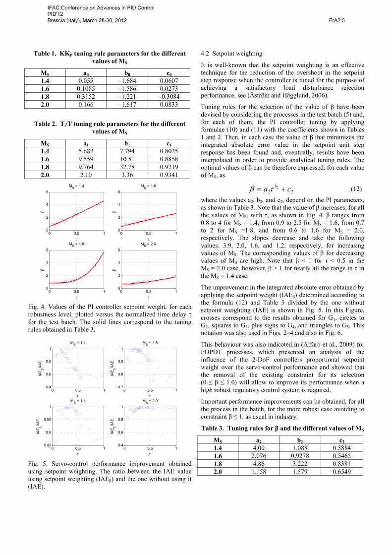
Table 1. KKP tuning rule parameters for the different values of MS

MS a0 b0 c0 1.4 0.055 –1.684 0.0607 1.6 0.1085 –1.586 0.0273 1.8 0.3152 –1.221 –0.3084 2.0 0.166 –1.617 0.0833

Table 2. Ti/T tuning rule parameters for the different values of MS

MS a1 b1 c1 1.4 5.682 7.794 0.8025 1.6 9.559 10.51 0.8858 1.8 9.764 32.78 0.9219 2.0 2.10 3.36 0.9341

Fig. 4. Values of the PI controller setpoint weight, for each robustness level, plotted versus the normalized time delay τ for the test batch. The solid lines correspond to the tuning rules obtained in Table 3.

Fig. 5. Servo-control performance improvement obtained using setpoint weighting. The ratio between the IAE value using setpoint weighting (IAEβ) and the one without using it (IAE).

4.2 Setpoint weighting

It is well-known that the setpoint weighting is an effective technique for the reduction of the overshoot in the setpoint step response when the controller is tuned for the purpose of achieving a satisfactory load disturbance rejection performance, see (Åström and Hägglund, 2006).

Tuning rules for the selection of the value of β have been devised by considering the processes in the test batch (5) and, for each of them, the PI controller tuning by applying formulae (10) and (11) with the coefficients shown in Tables 1 and 2. Then, in each case the value of β that minimizes the integrated absolute error value in the setpoint unit step response has been found and, eventually, results have been interpolated in order to provide analytical tuning rules. The optimal values of β can be therefore expressed, for each value of MS, as

222 ca b += τβ (12)

where the values a2, b2, and c2, depend on the PI parameters, as shown in Table 3. Note that the value of β increases, for all the values of MS, with τ, as shown in Fig. 4. β ranges from 0.8 to 4 for MS = 1.4, from 0.9 to 2.5 for MS = 1.6, from 0.7 to 2 for MS =1.8, and from 0.6 to 1.6 for MS = 2.0, respectively. The slopes decrease and take the following values: 3.9, 2.0, 1.6, and 1.2, respectively, for increasing values of MS. The corresponding values of β for decreasing values of MS are high. Note that β < 1 for τ < 0.5 in the MS = 2.0 case, however, β > 1 for nearly all the range in τ in the MS = 1.4 case.

The improvement in the integrated absolute error obtained by applying the setpoint weight (IAEβ) determined according to the formula (12) and Table 3 divided by the one without setpoint weighting (IAE) is shown in Fig. 5. In this Figure, crosses correspond to the results obtained for G1, circles to G2, squares to G3, plus signs to G4, and triangles to G5. This notation was also used in Figs. 2–4 and also in Fig. 6.

This behaviour was also indicated in (Alfaro et al., 2009) for FOPDT processes, which presented an analysis of the influence of the 2-DoF controllers proportional setpoint weight over the servo-control performance and showed that the removal of the existing constraint for its selection (0 ≤ β ≤ 1.0) will allow to improve its performance when a high robust regulatory control system is required.

Important performance improvements can be obtained, for all the process in the batch, for the more robust case avoiding to constraint β ≤ 1, as usual in industry.

Table 3. Tuning rules for β and the different values of MS

MS a2 b2 c2 1.4 4.00 1.088 0.5884 1.6 2.076 0.9278 0.5465 1.8 4.86 3.222 0.8381 2.0 1.158 1.579 0.6549

0 0.5 10

2

4

6MS = 1.4

τ

β

0 0.5 10

2

4

6MS = 1.6

τ

β

0 0.5 10

2

4

6MS = 1.8

τ

β

0 0.5 10

2

4

6MS = 2.0

τ

β

0 0.5 10.4

0.6

0.8

1MS = 1.4

τ

IAE β

/IAE

0 0.5 10.7

0.8

0.9

1MS = 1.6

τ

IAE β

/IAE

0 0.5 10.85

0.9

0.95

1MS = 1.8

τ

IAE β

/IAE

0 0.5 10.4

0.6

0.8

1MS = 2.0

τ

IAE β

/IAE

IFAC Conference on Advances in PID Control PID'12 Brescia (Italy), March 28-30, 2012 FrA2.5

Fig. 6. Normalized PI controller parameters plotted versus normalized dead time for the processes in the test batch. Parameters in blue correspond to the design parameter MS = 1.4, and parameters marked in red correspond to MS = 2.0. The ratios between the IAE value using setpoint weighting and the one without using it are also compared for both values of MS.

4.3 Comparison between rules for different robustness levels

The new simple tuning rules have been derived minimizing disturbance performance, using MS as a design parameter.

Figure 6 shows 2-DoF PI controller parameters, for a high (MS = 1.4) and a minimum level of robustness (MS = 2.0), in order to compare the effect of the robustness design parameter over the obtained controller parameters.

Figure 6 shows that the integration times are essentially the same for both values of MS. The controller gains have similar dependencies on τ but the gain obtained for minimum robustness (MS = 2.0) is about twice as high as the gain obtained for high robustness (MS = 1.4). This indicates that to obtain more aggressive control at the cost of lower robustness can be achieving simply by increasing the gain. An extremely simple tuning rule for PI controllers could be following expressions (11) and (12) together with Tables 2 and 3 for Ti and β parameters while K could be modified depending on the desired aggressiveness. However, following the proposed tuning rules for several robustness levels instead of modifying by trial and error the proportional gain, we guarantee the desired robustness level and respect the performance-robustness trade-off.

The value of β is approximately the same for both cases for very low values of τ, however, the slope increases nearly four times for the high robustness case.

The improvement in servo control using the setpoint weighting behaves in a different way depending on the robustness level. For a high level of robustness (MS = 1.4), note that for values of τ ≥ 0.15 the value of β is greater than 1.0. The improvement in using setpoint weighting grows towards 45% for delay-dominated processes and it is negligible for lag-dominated processes. This behaviour changes for increasing values of MS.

However, the behaviour is completely different for MS = 2.0. The improvement in lag-dominant processes grows towards 20%, the one for delay-dominated processes is reduced towards 3%, and the negligible improvement is moved progressively towards balanced lag and delay processes.

5. SIMULATION RESULTS

Consider a process with the transfer function:

( )411)(+

=s

sG (13)

Fitting the FOPDT model to the process we find that the apparent time delay and time constant are L = 1.42 and T = 2.90, respectively. Hence the controllability index is L/T = 0.5 and the normalized dead time is τ = 0.33.

The tuning rules for 2-DoF PI controllers proposed in this paper are compared in terms of IAE and MS with the Ziegler and Nichols step and frequency methods (ZN step and ZN frequency), Åström and Hägglund’s kappa-tau and AMIGO methods, and Alfaro’s PI2Ms tuning rules for the same robustness levels, respectively. See (Åström and Hägglund, 2006) and (Alfaro et al., 2010) for reference of all these methods.

Table 4 shows controller parameters, robustness and servo-regulation performance indices for all the tuning methods considered.

First of all, the benefit obtained in using the proposed setpoint weighting values can be quantified in 26%, 4%, 1%, and 2%, respectively, for increasing values of MS. This is in correlation to Fig. 5, which quantifies the improvement for the whole test batch.

A reduction of 16% and 18% in IAEβ has been obtained for the proposed method (MS = 1.4 and 2.0) in comparison with kappa tau tuning rules.

Related to disturbance rejection performance, kappa tau rules have a decrease of 4% in IAEd at the cost of a smaller robustness. However, a reduction of 20% in IAEd is obtained using the proposed method for MS = 2.0 in comparison with kappa tau method.

Otherwise, the reduction in IAEβ is 20%, 17%, 10%, and 7%, respectively, compared to Alfaro’s method for increasing values of MS. Similar or smaller values of IAEd are obtained for the proposed method in comparison to Alfaro’s method, what show the effectiveness of the proposed method.

Table 4 shows good results for the proposed tuning rules in comparison with classical and well-established modern methods.

6. CONCLUSIONS

This paper presents new tuning rules for 2-DoF PI controllers for several robustness levels in the spirit of the kappa-tau tuning rules for a test batch of typical processes found in process control. The rules are based on characterization of the process dynamics by three parameters, i.e. gain KP, apparent time constant T and apparent time delay L, that can be obtained by a simple step response experiment.

0 0.5 10

1

2

3

4

5

τ

KK

P

0 0.5 10

1

2

3

4

5

τT i/T

0 0.5 10

1

2

3

4

5

τ

β

0 0.5 10.4

0.6

0.8

1

τ

IAE β

/IAE

IFAC Conference on Advances in PID Control PID'12 Brescia (Italy), March 28-30, 2012 FrA2.5

Table 4. Controller parameters obtained with several design methods for a process with transfer function G(s) = 1/(s+1)4

Method K Ti β ki MS IAEd IAEr IAEβ IAEβ/IAEr Proposed (MS = 1.4) 0.43 2.35 1.78 0.18 1.38 5.40 5.55 4.09 0.74 Proposed (MS = 1.6) 0.66 2.59 1.28 0.26 1.59 3.90 4.12 3.98 0.96 Proposed (MS = 1.8) 0.92 2.70 0.97 0.34 1.87 3.20 4.10 4.09 0.99 Proposed (MS = 2.0) 1.09 2.88 0.85 0.38 2.05 3.02 4.23 4.14 0.98

Alfaro et al. (MS = 1.4) 0.54 2.90 1.05 0.19 1.39 5.38 - 5.12 - Alfaro et al. (MS = 1.6) 0.76 1.14 0.78 0.66 1.59 4.13 - 4.82 - Alfaro et al. (MS = 1.8) 0.92 3.20 0.66 0.29 1.76 3.49 - 4.52 - Alfaro et al. (MS = 2.0) 1.03 3.21 0.59 0.32 1.90 3.13 - 4.43 -

κτ (MS = 1.4) 0.36 1.89 1.26 0.19 1.41 5.19 5.25 4.87 0.93 κτ (MS = 2.0) 0.77 1.89 0.54 0.41 2.13 3.76 5.00 5.04 1.00

AMIGO (MS = 1.4) 0.51 2.3 1 0.22 1.47 4.54 4.56 4.56 1.00 ZN Step 1.85 4.27 1 0.43 3.25 2.85 5.34 5.34 1.00

ZN Frequency 1.61 5.01 1 0.32 2.48 3.11 4.30 4.30 1.00

The design method consists on minimizing IAE, for disturbance rejection, subject to a constraint on the maximum sensitivity function. Four robustness levels are proposed and tuning rules are obtained for those levels. Based on these parameters it is possible to develop very simple tuning rules for PI controllers that only depend on the normalized time delay τ.

In this paper it is also demonstrated that substantially better performance can be obtained using setpoint weighting without constraining its value. The benefit is quantified for the four proposed levels and for all the processes in the test batch.

These tuning rules are shown to give good results compared to a couple of well established classical and modern tuning methods, especially when simplicity, performance and robustness are emphasized.

Future investigation should rely on extending these tuning rules to integral processes and applied to PID and fractional PID controllers.

REFERENCES

Alfaro, V.M., Vilanova, R. and Arrieta, O. (2009). “Considerations on Set-Point Weight Choice for 2DoF PID Controllers”, in IFAC International Symposium on Advanced Control of Chemical Processes (IFAC ADCHEM 2009), Istambul, Turkey.

Alfaro, V.M., Vilanova, R. and Arrieta, O. (2010). “Maximum-Sensitivity Based Robust Tuning for Two-Degree-of-Freedom Proportional-Integral Controllers”, Industrial and Engineering Chemical Research, Vol. 49 (11), pp. 5415-5423.

Åström, K.J. and Hägglund, T. (1995). PID Controllers: Theory, Design, and Tuning, Instrument Society of America. Research Triangle Park, NC.

Åström, K.J. and Hägglund, T. (2000). “Benchmark systems for PID control”, Proceedings of IFAC workshop on Digital Control. Past, Present and Future of PID Control, pp. 165-166. Terrassa, Spain.

Åström, K.J. and Hägglund, T. (2001). “The future of PID control”, Control Engineering Practice, Vol. 9 (11), pp. 1163-1175.

Åström, K.J. and Hägglund, T. (2004). “Revisiting the Ziegler Nichols step response method for PID control”, Journal of Process Control, Vol. 14, pp. 635-640.

Åström, K.J. and Hägglund, T. (2006). Advanced PID control. Research Triangle Park, NC, Instrum. Soc. Amer.

Chien, K.L., Hrones, J.A., and Reswick, J.B., (1952). “On the automatic control of generalized passive systems”, Transactions ASME, Vol. 74, pp. 175-185.

Cohen, G.H. and Coon, G.A. (1953). “Theoretical consideration of retarded control”, Transactions ASME, Vol. 75, pp. 827-834.

Gorez, R. (2003). “New design relations for 2-DOF PID-like control systems”. Automatica, Vol. 39 (5), pp. 901-908.

Gude, J.J. and Kahoraho, E. (2007). “PID control: Current status and alternatives”, In 2nd Seminar for Advanced Industrial Control Applications – SAICA 2007, pp. 247-253, UNED Ediciones.

Hang, C.C, Åström, K.J. and Hägglund, T. (1991). “Refinements of the Ziegler-Nichols tuning formula”, IEE Proc.-Part D, Vol. 138 (2), pp. 111-118.

Shinskey, F.G. (1996). Process Control Systems. Application, design, and tuning. 4th edition. McGraw-Hill.

Vilanova, R. and Alfaro, V.M. (2011). “Robust PID control: an overview” (in Spanish), Revista Iberoamericana de Automática e Informática Industrial, Vol. 8, pp. 141-158.

Ziegler, J.G. and Nichols, N.B. (1942). “Optimum settings for automatic controllers”, Transactions ASME, Vol. 64, pp. 759-768.

IFAC Conference on Advances in PID Control PID'12 Brescia (Italy), March 28-30, 2012 FrA2.5