karl liechty joint work with dong wang and robert ... · pdf filekarl liechty nibm on circle....
TRANSCRIPT
Nonintersecting Brownian motions on the unit circle
Karl Liechtyjoint work with Dong Wang and Robert Buckingham
Painleve Equations and Applications: A Workshop in Memory of A. A. KapaevAugust 27, 2017
Karl Liechty NIBM on circle
Nonintersecting paths and determinantal processes
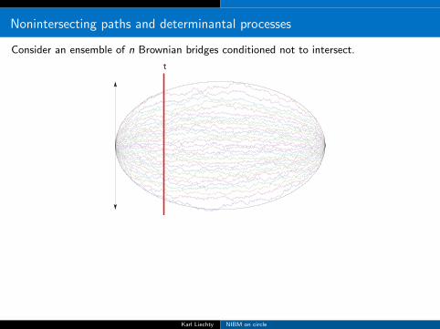
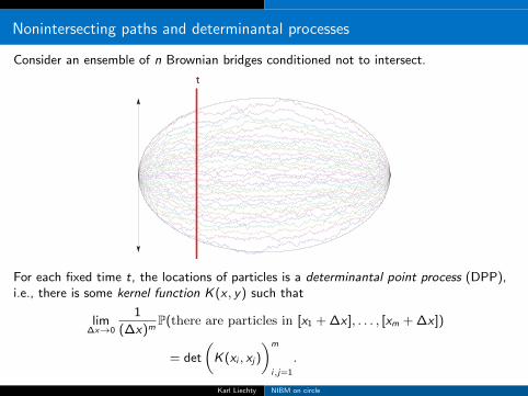
Consider an ensemble of n Brownian bridges conditioned not to intersect.
t
For each fixed time t, the locations of particles is a determinantal point process (DPP),i.e., there is some kernel function K(x , y) such that
lim∆x→0
1
(∆x)mP(there are particles in [x1 + ∆x ], . . . , [xm + ∆x ])
= det
(K(xi , xj)
)m
i,j=1
.
Karl Liechty NIBM on circle
Nonintersecting paths and determinantal processes
Consider an ensemble of n Brownian bridges conditioned not to intersect.
t
For each fixed time t, the locations of particles is a determinantal point process (DPP),i.e., there is some kernel function K(x , y) such that
lim∆x→0
1
(∆x)mP(there are particles in [x1 + ∆x ], . . . , [xm + ∆x ])
= det
(K(xi , xj)
)m
i,j=1
.
Karl Liechty NIBM on circle
Nonintersecting Brownian bridges
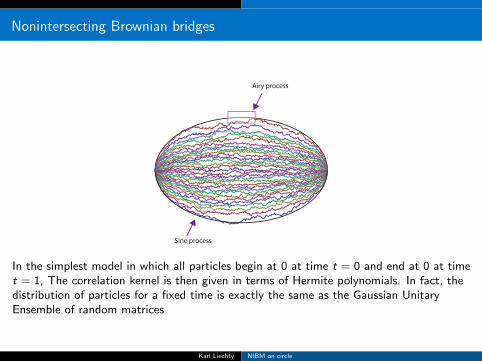
Airy process
Sine process
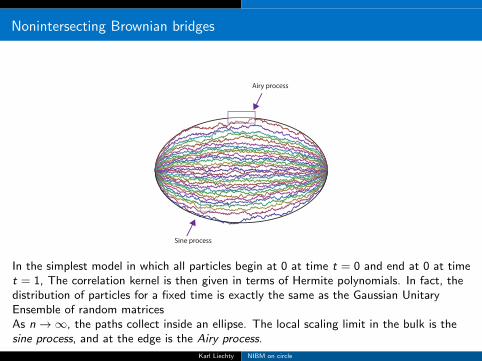
In the simplest model in which all particles begin at 0 at time t = 0 and end at 0 at timet = 1, The correlation kernel is then given in terms of Hermite polynomials. In fact, thedistribution of particles for a fixed time is exactly the same as the Gaussian UnitaryEnsemble of random matrices
As n→∞, the paths collect inside an ellipse. The local scaling limit in the bulk is thesine process, and at the edge is the Airy process.
Karl Liechty NIBM on circle
Nonintersecting Brownian bridges
Airy process
Sine process
In the simplest model in which all particles begin at 0 at time t = 0 and end at 0 at timet = 1, The correlation kernel is then given in terms of Hermite polynomials. In fact, thedistribution of particles for a fixed time is exactly the same as the Gaussian UnitaryEnsemble of random matricesAs n→∞, the paths collect inside an ellipse. The local scaling limit in the bulk is thesine process, and at the edge is the Airy process.
Karl Liechty NIBM on circle

Other limiting processes
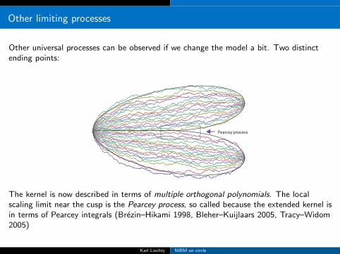
Other universal processes can be observed if we change the model a bit.
Two distinctending points:
Pearcey process
The kernel is now described in terms of multiple orthogonal polynomials. The localscaling limit near the cusp is the Pearcey process, so called because the extended kernel isin terms of Pearcey integrals (Brezin–Hikami 1998, Bleher–Kuijlaars 2005, Tracy–Widom2005)
Karl Liechty NIBM on circle
Other limiting processes
Other universal processes can be observed if we change the model a bit. Two distinctending points:
Pearcey process
The kernel is now described in terms of multiple orthogonal polynomials. The localscaling limit near the cusp is the Pearcey process, so called because the extended kernel isin terms of Pearcey integrals (Brezin–Hikami 1998, Bleher–Kuijlaars 2005, Tracy–Widom2005)
Karl Liechty NIBM on circle
Other limiting processes
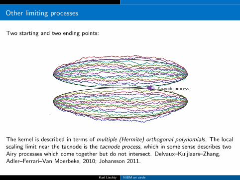
Two starting and two ending points:
Tacnode process
The kernel is described in terms of multiple (Hermite) orthogonal polynomials. The localscaling limit near the tacnode is the tacnode process, which in some sense describes twoAiry processes which come together but do not intersect. Delvaux–Kuijlaars–Zhang,Adler–Ferrari–Van Moerbeke, 2010; Johansson 2011.
Karl Liechty NIBM on circle
Deformations of these processes
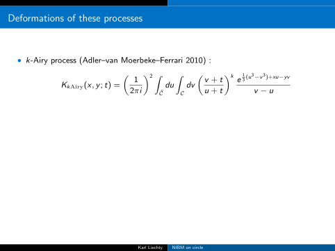
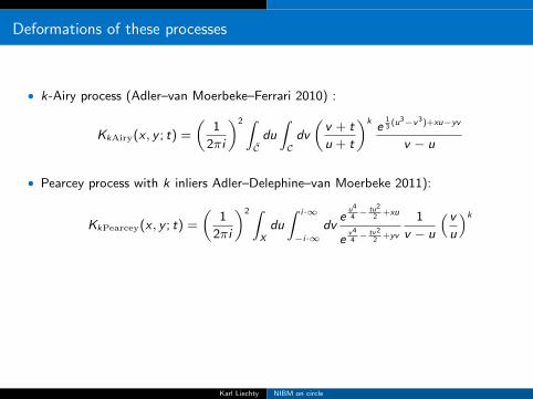
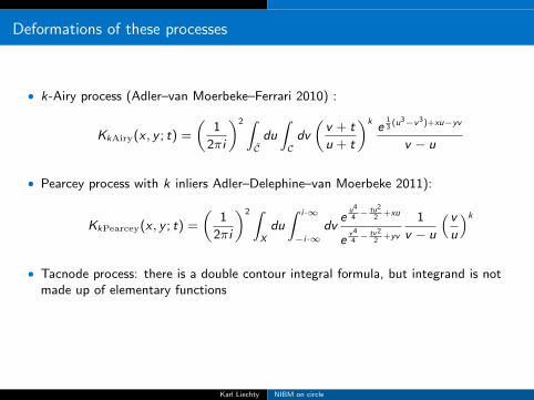
• k-Airy process (Adler–van Moerbeke–Ferrari 2010) :
KkAiry(x , y ; t) =
(1
2πi
)2 ∫Cdu
∫Cdv
(v + t
u + t
)ke
13
(u3−v3)+xu−yv
v − u
• Pearcey process with k inliers Adler–Delephine–van Moerbeke 2011):
KkPearcey(x , y ; t) =
(1
2πi
)2 ∫X
du
∫ i·∞
−i·∞dv
eu4
4− tu2
2+xu
ev4
4− tv2
2+yv
1
v − u
(vu
)k• Tacnode process: there is a double contour integral formula, but integrand is not
made up of elementary functions
• In each case, “shape” of kernel is amenable to Bertola–Caffaso-type analysis(Girotti’s talk yesterday)
Karl Liechty NIBM on circle
Deformations of these processes
• k-Airy process (Adler–van Moerbeke–Ferrari 2010) :
KkAiry(x , y ; t) =
(1
2πi
)2 ∫Cdu
∫Cdv
(v + t
u + t
)ke
13
(u3−v3)+xu−yv
v − u
• Pearcey process with k inliers Adler–Delephine–van Moerbeke 2011):
KkPearcey(x , y ; t) =
(1
2πi
)2 ∫X
du
∫ i·∞
−i·∞dv
eu4
4− tu2
2+xu
ev4
4− tv2
2+yv
1
v − u
(vu
)k
• Tacnode process: there is a double contour integral formula, but integrand is notmade up of elementary functions
• In each case, “shape” of kernel is amenable to Bertola–Caffaso-type analysis(Girotti’s talk yesterday)
Karl Liechty NIBM on circle
Deformations of these processes
• k-Airy process (Adler–van Moerbeke–Ferrari 2010) :
KkAiry(x , y ; t) =
(1
2πi
)2 ∫Cdu
∫Cdv
(v + t
u + t
)ke
13
(u3−v3)+xu−yv
v − u
• Pearcey process with k inliers Adler–Delephine–van Moerbeke 2011):
KkPearcey(x , y ; t) =
(1
2πi
)2 ∫X
du
∫ i·∞
−i·∞dv
eu4
4− tu2
2+xu
ev4
4− tv2
2+yv
1
v − u
(vu
)k• Tacnode process: there is a double contour integral formula, but integrand is not
made up of elementary functions
• In each case, “shape” of kernel is amenable to Bertola–Caffaso-type analysis(Girotti’s talk yesterday)
Karl Liechty NIBM on circle
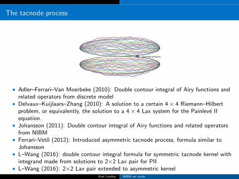
The tacnode process
Tacnode process
• Adler–Ferrari–Van Moerbeke (2010): Double contour integral of Airy functions andrelated operators from discrete model
• Delvaux–Kuijlaars–Zhang (2010): A solution to a certain 4× 4 Riemann–Hilbertproblem, or equivalently, the solution to a 4× 4 Lax system for the Painleve IIequation.
• Johansson (2011): Double contour integral of Airy functions and related operatorsfrom NIBM
• Ferrari–Veto (2012): Introduced asymmetric tacnode process, formula similar toJohansson
• L–Wang (2016): double contour integral formula for symmetric tacnode kernel withintegrand made from solutions to 2×2 Lax pair for PII
• L–Wang (2016): 2×2 Lax pair extended to asymmetric kernelKarl Liechty NIBM on circle
A double contour integral formula for tacnode kernel
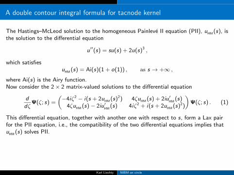
The Hastings–McLeod solution to the homogeneous Painleve II equation (PII), uHM (s), isthe solution to the differential equation
u′′(s) = su(s) + 2u(s)3 ,
which satisfiesuHM (s) = Ai(s)(1 + o(1)) , as s → +∞ ,
where Ai(s) is the Airy function.
Now consider the 2× 2 matrix-valued solutions to the differential equation
d
dζΨ(ζ; s) =
(−4iζ2 − i(s + 2uHM (s)2) 4ζuHM (s) + 2iu′
HM(s)
4ζuHM (s)− 2iu′HM
(s) 4iζ2 + i(s + 2uHM (s)2)
)Ψ(ζ; s) . (1)
This differential equation, together with another one with respect to s, form a Lax pairfor the PII equation, i.e., the compatibility of the two differential equations implies thatuHM (s) solves PII.We consider the particular solution to (1) which satisfies
Ψ(ζ; s)e i(43ζ3+sζ)σ3 = I + O(ζ−1) , ζ → ±∞ .
Karl Liechty NIBM on circle
A double contour integral formula for tacnode kernel
The Hastings–McLeod solution to the homogeneous Painleve II equation (PII), uHM (s), isthe solution to the differential equation
u′′(s) = su(s) + 2u(s)3 ,
which satisfiesuHM (s) = Ai(s)(1 + o(1)) , as s → +∞ ,
where Ai(s) is the Airy function.Now consider the 2× 2 matrix-valued solutions to the differential equation
d
dζΨ(ζ; s) =
(−4iζ2 − i(s + 2uHM (s)2) 4ζuHM (s) + 2iu′
HM(s)
4ζuHM (s)− 2iu′HM
(s) 4iζ2 + i(s + 2uHM (s)2)
)Ψ(ζ; s) . (1)
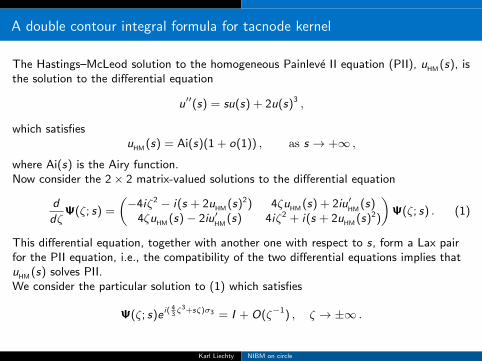
This differential equation, together with another one with respect to s, form a Lax pairfor the PII equation, i.e., the compatibility of the two differential equations implies thatuHM (s) solves PII.
We consider the particular solution to (1) which satisfies
Ψ(ζ; s)e i(43ζ3+sζ)σ3 = I + O(ζ−1) , ζ → ±∞ .
Karl Liechty NIBM on circle
A double contour integral formula for tacnode kernel
The Hastings–McLeod solution to the homogeneous Painleve II equation (PII), uHM (s), isthe solution to the differential equation
u′′(s) = su(s) + 2u(s)3 ,
which satisfiesuHM (s) = Ai(s)(1 + o(1)) , as s → +∞ ,
where Ai(s) is the Airy function.Now consider the 2× 2 matrix-valued solutions to the differential equation
d
dζΨ(ζ; s) =
(−4iζ2 − i(s + 2uHM (s)2) 4ζuHM (s) + 2iu′
HM(s)
4ζuHM (s)− 2iu′HM
(s) 4iζ2 + i(s + 2uHM (s)2)
)Ψ(ζ; s) . (1)
This differential equation, together with another one with respect to s, form a Lax pairfor the PII equation, i.e., the compatibility of the two differential equations implies thatuHM (s) solves PII.We consider the particular solution to (1) which satisfies
Ψ(ζ; s)e i(43ζ3+sζ)σ3 = I + O(ζ−1) , ζ → ±∞ .
Karl Liechty NIBM on circle
A double contour integral formula for tacnode kernel
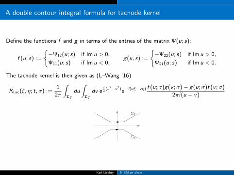
Define the functions f and g in terms of the entries of the matrix Ψ(u; s):
f (u; s) :=
{−Ψ12(u; s) if Im u > 0,
Ψ11(u; s) if Im u < 0,g(u, s) :=
{−Ψ22(u; s) if Im u > 0,
Ψ21(u; s) if Im u < 0.
The tacnode kernel is then given as (L–Wang ’16)
Ktac(ξ, η; t, σ) :=1
2π
∫ΣT
du
∫ΣT
dv et2
(u2−v2)e−i(uξ−vη) f (u;σ)g(v ;σ)− g(u;σ)f (v ;σ)
2πi(u − v)
ΣT
ΣT
Karl Liechty NIBM on circle
A deformation of the tacnode process
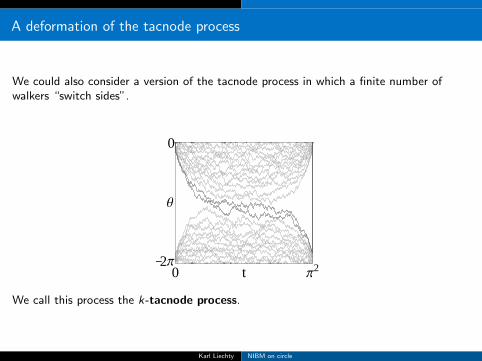
We could also consider a version of the tacnode process in which a finite number ofwalkers “switch sides”.
0
Θ
Π
0 t Π2
_2
We call this process the k-tacnode process.
Karl Liechty NIBM on circle
The generalized Hastings–McLeod solution to PII
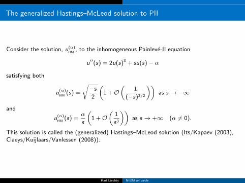
Consider the solution, u(α)HM
, to the inhomogeneous Painleve-II equation
u′′(s) = 2u(s)3 + su(s)− α
satisfying both
u(α)HM
(s) =
√−s2
(1 +O
(1
(−s)3/2
))as s → −∞
and
u(α)HM
(s) =α
s
(1 +O
(1
s3
))as s → +∞ (α 6= 0).
This solution is called the (generalized) Hastings–McLeod solution (Its/Kapaev (2003),Claeys/Kuijlaars/Vanlessen (2008)).
Karl Liechty NIBM on circle
The τ -functions for HM solution to PII
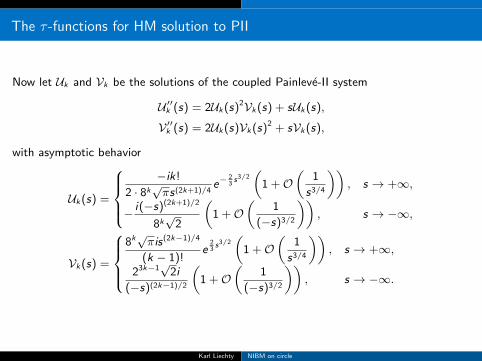
Now let Uk and Vk be the solutions of the coupled Painleve-II system
U ′′k (s) = 2Uk(s)2Vk(s) + sUk(s),
V ′′k (s) = 2Uk(s)Vk(s)2 + sVk(s),
with asymptotic behavior
Uk(s) =
−ik!
2 · 8k√πs(2k+1)/4
e−23s3/2(
1 +O(
1
s3/4
)), s → +∞,
− i(−s)(2k+1)/2
8k√
2
(1 +O
(1
(−s)3/2
)), s → −∞,
Vk(s) =
8k√πis(2k−1)/4
(k − 1)!e
23s3/2(
1 +O(
1
s3/4
)), s → +∞,
23k−1√
2i
(−s)(2k−1)/2
(1 +O
(1
(−s)3/2
)), s → −∞.
Karl Liechty NIBM on circle
The τ -functions for HM solution to PII
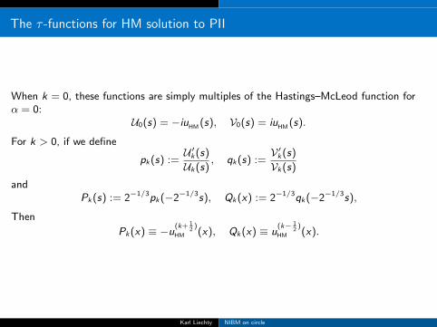
When k = 0, these functions are simply multiples of the Hastings–McLeod function forα = 0:
U0(s) = −iuHM (s), V0(s) = iuHM (s).
For k > 0, if we define
pk(s) :=U ′k(s)
Uk(s), qk(s) :=
V ′k(s)
Vk(s)
andPk(s) := 2−1/3pk(−2−1/3s), Qk(x) := 2−1/3qk(−2−1/3s),
Then
Pk(x) ≡ −u(k+ 12
)HM (x), Qk(x) ≡ u
(k− 12
)HM (x).
Karl Liechty NIBM on circle
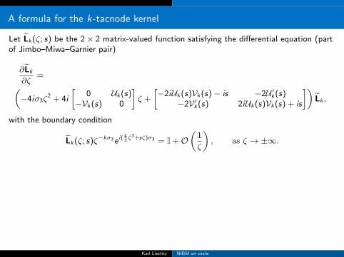
A formula for the k-tacnode kernel
Let Lk(ζ; s) be the 2× 2 matrix-valued function satisfying the differential equation (partof Jimbo–Miwa–Garnier pair)
∂Lk
∂ζ=(
−4iσ3ζ2 + 4i
[0 Uk(s)
−Vk(s) 0
]ζ +
[−2iUk(s)Vk(s)− is −2U ′k(s)
−2V ′k(s) 2iUk(s)Vk(s) + is
])Lk ,
with the boundary condition
Lk(ζ; s)ζ−kσ3e i(43ζ3+sζ)σ3 = I +O
(1
ζ
), as ζ → ±∞.
Then define the functions
fk(u; s) :=
{−[Lk(u; s)]12, Im u > 0,
[Lk(u; s)]11, Im u < 0,gk(u; s) :=
{−[Lk(u; s)]22, Im u > 0,
[Lk(u; s)]21, Im u < 0.
The k-tacnode kernel is then (Buckingham–L. 2017)
K(k)tac(ξ, η;σ, t) :=
1
2π
∫ΣT
du
∫ΣT
dv et2
(u2−v2)−i(ξu−ηv) fk(u;σ)gk(v ;σ)− gk(u;σ)fk(v ;σ)
2πi(u − v).
Karl Liechty NIBM on circle
A formula for the k-tacnode kernel
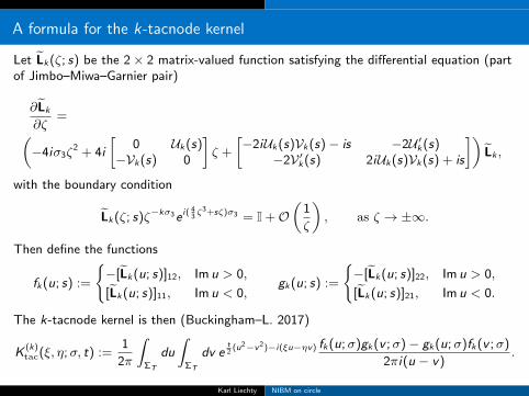
Let Lk(ζ; s) be the 2× 2 matrix-valued function satisfying the differential equation (partof Jimbo–Miwa–Garnier pair)
∂Lk
∂ζ=(
−4iσ3ζ2 + 4i
[0 Uk(s)
−Vk(s) 0
]ζ +
[−2iUk(s)Vk(s)− is −2U ′k(s)
−2V ′k(s) 2iUk(s)Vk(s) + is
])Lk ,
with the boundary condition
Lk(ζ; s)ζ−kσ3e i(43ζ3+sζ)σ3 = I +O
(1
ζ
), as ζ → ±∞.
Then define the functions
fk(u; s) :=
{−[Lk(u; s)]12, Im u > 0,
[Lk(u; s)]11, Im u < 0,gk(u; s) :=
{−[Lk(u; s)]22, Im u > 0,
[Lk(u; s)]21, Im u < 0.
The k-tacnode kernel is then (Buckingham–L. 2017)
K(k)tac(ξ, η;σ, t) :=
1
2π
∫ΣT
du
∫ΣT
dv et2
(u2−v2)−i(ξu−ηv) fk(u;σ)gk(v ;σ)− gk(u;σ)fk(v ;σ)
2πi(u − v).
Karl Liechty NIBM on circle
Nonintersecting Brownian motions on the circle
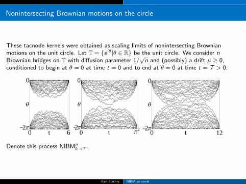
These tacnode kernels were obtained as scaling limits of nonintersecting Brownianmotions on the unit circle. Let T = {e iθ|θ ∈ R} be the unit circle. We consider nBrownian bridges on T with diffusion parameter 1/
√n and (possibly) a drift µ ≥ 0,
conditioned to begin at θ = 0 at time t = 0 and to end at θ = 0 at time t = T > 0.
2
Θ
0
0 t 6Π
_
0
Θ
0 t Π22_ Π
0
Θ
Π
0 t 12_2
Denote this process NIBMµ0→T .
Karl Liechty NIBM on circle
The kernel for NIBM on T
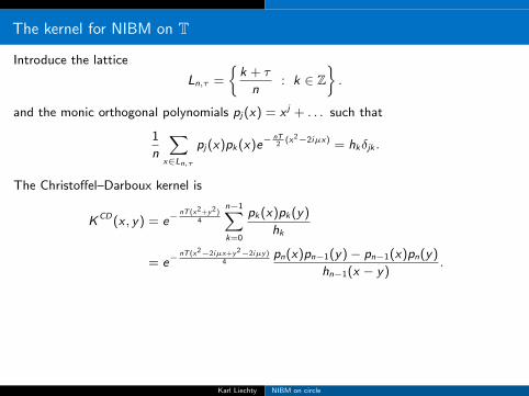
Introduce the lattice
Ln,τ =
{k + τ
n: k ∈ Z
}.
and the monic orthogonal polynomials pj(x) = x j + . . . such that
1
n
∑x∈Ln,τ
pj(x)pk(x)e−nT2
(x2−2iµx) = hkδjk .
The Christoffel–Darboux kernel is
KCD(x , y) = e−nT (x2+y2)
4
n−1∑k=0
pk(x)pk(y)
hk
= e−nT (x2−2iµx+y2−2iµy)
4pn(x)pn−1(y)− pn−1(x)pn(y)
hn−1(x − y).
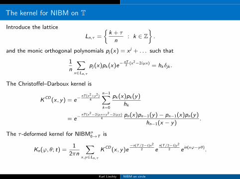
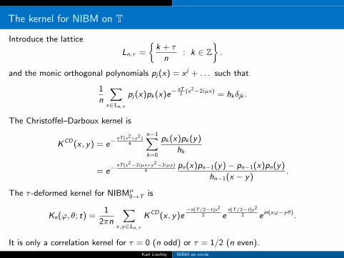
The τ -deformed kernel for NIBMµ0→T is
Kn(ϕ, θ; t) =1
2πn
∑x,y∈Ln,τ
KCD(x , y)e−n(T/2−t)x2
2 en(T/2−t)y2
2 e in(xϕ−yθ).
It is only a correlation kernel for τ = 0 (n odd) or τ = 1/2 (n even).
Karl Liechty NIBM on circle
The kernel for NIBM on T
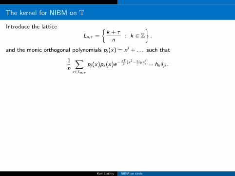
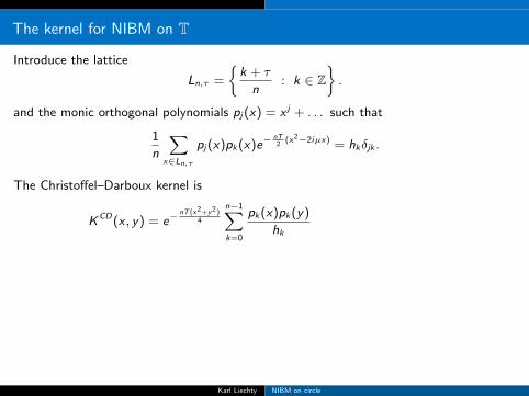
Introduce the lattice
Ln,τ =
{k + τ
n: k ∈ Z
}.
and the monic orthogonal polynomials pj(x) = x j + . . . such that
1
n
∑x∈Ln,τ
pj(x)pk(x)e−nT2
(x2−2iµx) = hkδjk .
The Christoffel–Darboux kernel is
KCD(x , y) = e−nT (x2+y2)
4
n−1∑k=0
pk(x)pk(y)
hk
= e−nT (x2−2iµx+y2−2iµy)
4pn(x)pn−1(y)− pn−1(x)pn(y)
hn−1(x − y).
The τ -deformed kernel for NIBMµ0→T is
Kn(ϕ, θ; t) =1
2πn
∑x,y∈Ln,τ
KCD(x , y)e−n(T/2−t)x2
2 en(T/2−t)y2
2 e in(xϕ−yθ).
It is only a correlation kernel for τ = 0 (n odd) or τ = 1/2 (n even).
Karl Liechty NIBM on circle
The kernel for NIBM on T
Introduce the lattice
Ln,τ =
{k + τ
n: k ∈ Z
}.
and the monic orthogonal polynomials pj(x) = x j + . . . such that
1
n
∑x∈Ln,τ
pj(x)pk(x)e−nT2
(x2−2iµx) = hkδjk .
The Christoffel–Darboux kernel is
KCD(x , y) = e−nT (x2+y2)
4
n−1∑k=0
pk(x)pk(y)
hk
= e−nT (x2−2iµx+y2−2iµy)
4pn(x)pn−1(y)− pn−1(x)pn(y)
hn−1(x − y).
The τ -deformed kernel for NIBMµ0→T is
Kn(ϕ, θ; t) =1
2πn
∑x,y∈Ln,τ
KCD(x , y)e−n(T/2−t)x2
2 en(T/2−t)y2
2 e in(xϕ−yθ).
It is only a correlation kernel for τ = 0 (n odd) or τ = 1/2 (n even).Karl Liechty NIBM on circle
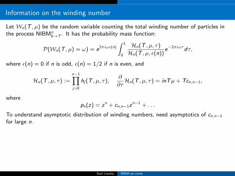
Information on the winding number
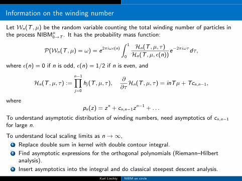
Let Wn(T , µ) be the random variable counting the total winding number of particles inthe process NIBMµ
0→T . It has the probability mass function:
P(Wn(T , µ) = ω) = e2πiωε(n)
∫ 1
0
Hn(T , µ, τ)
Hn(T , µ, ε(n))e−2πiωτdτ,
where ε(n) = 0 if n is odd, ε(n) = 1/2 if n is even, and
Hn(T , µ, τ) :=n−1∏j=0
hj(T , µ, τ),∂
∂τHn(T , µ, τ) = inTµ+ Tcn,n−1,
wherepn(z) = zn + cn,n−1z
n−1 + . . .
To understand asymptotic distribution of winding numbers, need asymptotics of cn,n−1
for large n.
To understand local scaling limits as n→∞,
1 Replace double sum in kernel with double contour integral.
2 Find asymptotic expressions for the orthogonal polynomials (Riemann–Hilbertanalysis).
3 Insert asymptotics into the integral and do classical steepest descent analysis.
Karl Liechty NIBM on circle
Information on the winding number
Let Wn(T , µ) be the random variable counting the total winding number of particles inthe process NIBMµ
0→T . It has the probability mass function:
P(Wn(T , µ) = ω) = e2πiωε(n)
∫ 1
0
Hn(T , µ, τ)
Hn(T , µ, ε(n))e−2πiωτdτ,
where ε(n) = 0 if n is odd, ε(n) = 1/2 if n is even, and
Hn(T , µ, τ) :=n−1∏j=0
hj(T , µ, τ),∂
∂τHn(T , µ, τ) = inTµ+ Tcn,n−1,
wherepn(z) = zn + cn,n−1z
n−1 + . . .
To understand asymptotic distribution of winding numbers, need asymptotics of cn,n−1
for large n.
To understand local scaling limits as n→∞,
1 Replace double sum in kernel with double contour integral.
2 Find asymptotic expressions for the orthogonal polynomials (Riemann–Hilbertanalysis).
3 Insert asymptotics into the integral and do classical steepest descent analysis.
Karl Liechty NIBM on circle
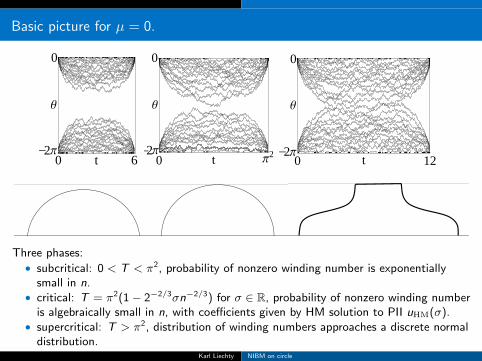
Basic picture for µ = 0.
2
Θ
0
0 t 6Π
_
0
Θ
0 t Π22_ Π
0
Θ
Π
0 t 12_2
Three phases:• subcritical: 0 < T < π2, probability of nonzero winding number is exponentially
small in n.• critical: T = π2(1− 2−2/3σn−2/3) for σ ∈ R, probability of nonzero winding number
is algebraically small in n, with coefficients given by HM solution to PII uHM(σ).• supercritical: T > π2, distribution of winding numbers approaches a discrete normal
distribution.Karl Liechty NIBM on circle
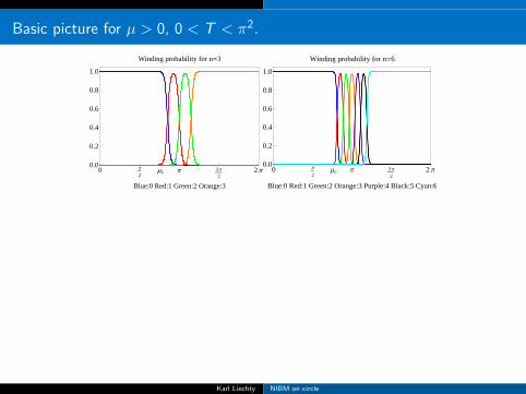
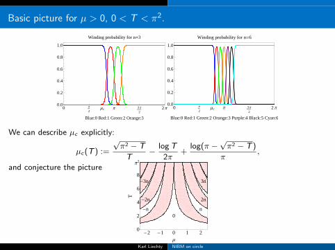
Basic picture for µ > 0, 0 < T < π2.
0 Π
2Μc Π 3 Π
22 Π
0.0
0.2
0.4
0.6
0.8
1.0
Blue:0 Red:1 Green:2 Orange:3
Winding probability for n=3
0 Π
2Μc Π 3 Π
22 Π
0.0
0.2
0.4
0.6
0.8
1.0
Blue:0 Red:1 Green:2 Orange:3 Purple:4 Black:5 Cyan:6
Winding probability for n=6
We can describe µc explicitly:
µc(T ) :=
√π2 − T
T− logT
2π+
log(π −√π2 − T )
π,
and conjecture the picture
0n-n
-2n 2n
3n-3n
-2 -1 0 1 20
2
4
6
8
Π2
Μ
T
Karl Liechty NIBM on circle
Rigorous results for 0 < T < π2
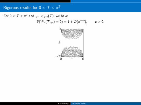
For 0 < T < π2 and |µ| < µc(T ), we have
P(Wn(T , µ) = 0) = 1 +O(e−cn), c > 0.
2
Θ
0
0 t 6Π
_
For µ just a bit bigger than µc , we see the winding number start to increase:
2 Π
Θ
00 t 6
Karl Liechty NIBM on circle
Rigorous results for 0 < T < π2
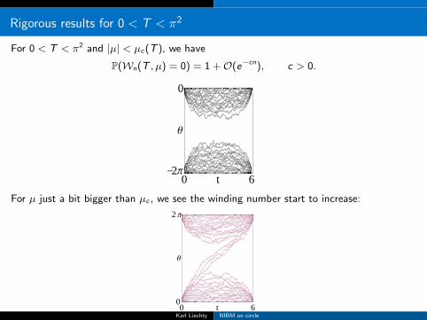
For 0 < T < π2 and |µ| < µc(T ), we have
P(Wn(T , µ) = 0) = 1 +O(e−cn), c > 0.
2
Θ
0
0 t 6Π
_
For µ just a bit bigger than µc , we see the winding number start to increase:
2 Π
Θ
00 t 6
Karl Liechty NIBM on circle
Rigorous results for 0 < T < π2
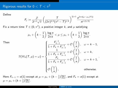
Define
Fj :=j!
2j+1√π
(T
(2π)3/2(π2 − T )1/4
)2j+1e2πn(µ−µc (T ))
nj+(1/2)
Fix a return time T ∈ (0, π2), a positive integer k, and µ satisfying
µc +
(k − 1
2
)log n
2πn< µ ≤ µc +
(k +
1
2
)log n
2πn.
Then
P(Wn(T , µ) = ω) =
F−1k−1
1 + Fk + F−1k−1
+O(
1
n
), ω = k − 1,
1
1 + Fk + F−1k−1
+O(
1
n
), ω = k,
Fk
1 + Fk + F−1k−1
+O(
1
n
), ω = k + 1,
O(
1
n
), otherwise.
.
Here Fk−1 = o(1) except at µ = µc + (k − 12) log n
2πn, and Fk = o(1) except at
µ = µc + (k + 12) log n
2πn.
Karl Liechty NIBM on circle
Rigorous results for T ≈ π2
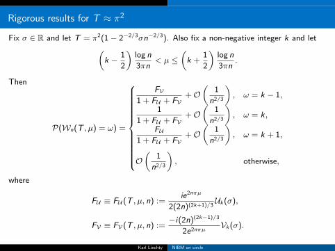
Fix σ ∈ R and let T = π2(1− 2−2/3σn−2/3). Also fix a non-negative integer k and let(k − 1
2
)log n
3πn< µ ≤
(k +
1
2
)log n
3πn.
Then
P(Wn(T , µ) = ω) =
FV1 + FU + FV
+O(
1
n2/3
), ω = k − 1,
1
1 + FU + FV+O
(1
n2/3
), ω = k,
FU1 + FU + FV
+O(
1
n2/3
), ω = k + 1,
O(
1
n2/3
), otherwise,
where
FU ≡ FU (T , µ, n) :=ie2nπµ
2(2n)(2k+1)/3Uk(σ),
FV ≡ FV(T , µ, n) :=−i(2n)(2k−1)/3
2e2nπµVk(σ).
Karl Liechty NIBM on circle
Rigorous results for T ≈ π2
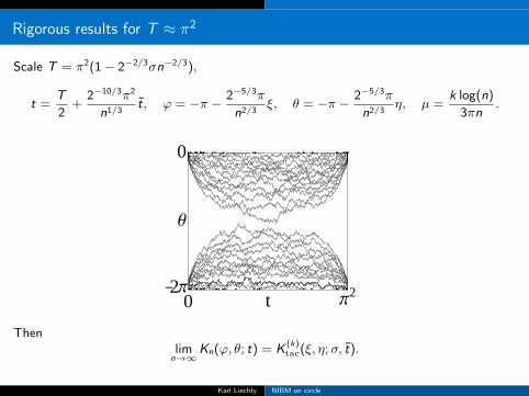
Scale T = π2(1− 2−2/3σn−2/3),
t =T
2+
2−10/3π2
n1/3t, ϕ = −π − 2−5/3π
n2/3ξ, θ = −π − 2−5/3π
n2/3η, µ =
k log(n)
3πn.
0
Θ
0 t Π22_ Π
Thenlim
n→∞Kn(ϕ, θ; t) = K
(k)tac(ξ, η;σ, t).
Karl Liechty NIBM on circle
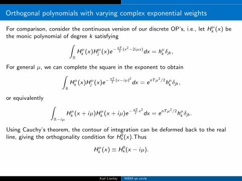
Orthogonal polynomials with varying complex exponential weights
For comparison, consider the continuous version of our discrete OP’s, i.e., let Hµk (x) bethe monic polynomial of degree k satisfying∫
RHµk (x)Hµj (x)e−
nT2
(x2−2iµx)dx = hµk δjk ,
For general µ, we can complete the square in the exponent to obtain∫RHµk (x)Hµj (x)e−
nT2
(x−iµ)2
dx = enTµ2/2hµk δjk ,
or equivalently ∫R−iµ
Hµk (x + iµ)Hµk (x + iµ)e−nT2
x2
dx = enTµ2/2hµk δjk .
Using Cauchy’s theorem, the contour of integration can be deformed back to the realline, giving the orthogonality condition for H0
k (x).Thus
Hµk (x) ≡ H0k (x − iµ).
For discrete weights, there is no way to use Cauchy’s theorem, so there is no suchrelation.
Karl Liechty NIBM on circle
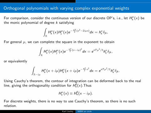
Orthogonal polynomials with varying complex exponential weights
For comparison, consider the continuous version of our discrete OP’s, i.e., let Hµk (x) bethe monic polynomial of degree k satisfying∫
RHµk (x)Hµj (x)e−
nT2
(x2−2iµx)dx = hµk δjk ,
For general µ, we can complete the square in the exponent to obtain∫RHµk (x)Hµj (x)e−
nT2
(x−iµ)2
dx = enTµ2/2hµk δjk ,
or equivalently ∫R−iµ
Hµk (x + iµ)Hµk (x + iµ)e−nT2
x2
dx = enTµ2/2hµk δjk .
Using Cauchy’s theorem, the contour of integration can be deformed back to the realline, giving the orthogonality condition for H0
k (x).Thus
Hµk (x) ≡ H0k (x − iµ).
For discrete weights, there is no way to use Cauchy’s theorem, so there is no suchrelation.
Karl Liechty NIBM on circle
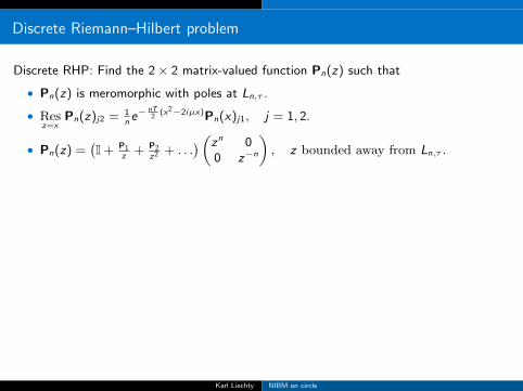
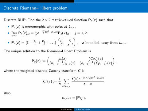
Discrete Riemann–Hilbert problem
Discrete RHP: Find the 2× 2 matrix-valued function Pn(z) such that
• Pn(z) is meromorphic with poles at Ln,τ .
• Resz=x
Pn(z)j2 = 1ne−
nT2
(x2−2iµx)Pn(x)j1, j = 1, 2.
• Pn(z) =(I + P1
z+ P2
z2 + . . .)(zn 0
0 z−n
), z bounded away from Ln,τ .
The unique solution to the Riemann-Hilbert Problem is
Pn(z) :=
(pn(z) (Cpn) (z)
(hn−1)−1pn−1(z) (hn−1)−1 (Cpn−1) (z)
),
where the weighted discrete Cauchy transform C is
Cf (z) :=1
n
∑x∈Ln,τ
f (x)e−(nT/2)(x2−2iµx)
z − x.
Also:cn,n−1 = [P1]11.
Karl Liechty NIBM on circle
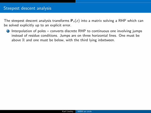
Steepest descent analysis
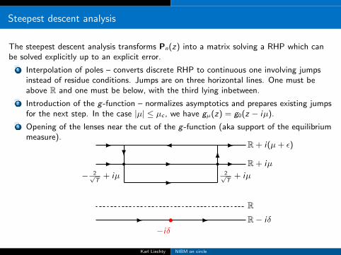
The steepest descent analysis transforms Pn(z) into a matrix solving a RHP which canbe solved explicitly up to an explicit error.
1 Interpolation of poles – converts discrete RHP to continuous one involving jumpsinstead of residue conditions. Jumps are on three horizontal lines. One must beabove R and one must be below, with the third lying inbetween.
2 Introduction of the g -function – normalizes asymptotics and prepares existing jumpsfor the next step. In the case |µ| ≤ µc , we have gµ(z) = g0(z − iµ).
3 Opening of the lenses near the cut of the g -function (aka support of the equilibriummeasure).
R
R + iµ
R + i(µ+ ε)
R− iδ
r r− 2√
T+ iµ 2√
T+ iµ
�
--
--
-
-
- -
6?
s−iδ
Karl Liechty NIBM on circle
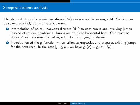
Steepest descent analysis
The steepest descent analysis transforms Pn(z) into a matrix solving a RHP which canbe solved explicitly up to an explicit error.
1 Interpolation of poles – converts discrete RHP to continuous one involving jumpsinstead of residue conditions. Jumps are on three horizontal lines. One must beabove R and one must be below, with the third lying inbetween.
2 Introduction of the g -function – normalizes asymptotics and prepares existing jumpsfor the next step. In the case |µ| ≤ µc , we have gµ(z) = g0(z − iµ).
3 Opening of the lenses near the cut of the g -function (aka support of the equilibriummeasure).
R
R + iµ
R + i(µ+ ε)
R− iδ
r r− 2√
T+ iµ 2√
T+ iµ
�
--
--
-
-
- -
6?
s−iδ
Karl Liechty NIBM on circle
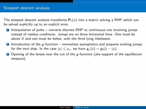
Steepest descent analysis
The steepest descent analysis transforms Pn(z) into a matrix solving a RHP which canbe solved explicitly up to an explicit error.
1 Interpolation of poles – converts discrete RHP to continuous one involving jumpsinstead of residue conditions. Jumps are on three horizontal lines. One must beabove R and one must be below, with the third lying inbetween.
2 Introduction of the g -function – normalizes asymptotics and prepares existing jumpsfor the next step. In the case |µ| ≤ µc , we have gµ(z) = g0(z − iµ).
3 Opening of the lenses near the cut of the g -function (aka support of the equilibriummeasure).
R
R + iµ
R + i(µ+ ε)
R− iδ
r r− 2√
T+ iµ 2√
T+ iµ
�
--
--
-
-
- -
6?
s−iδ
Karl Liechty NIBM on circle
Steepest descent analysis, 0 < T < π2
R
R + iµ
R + i(µ+ ε)
R− iδ
r r− 2√
T+ iµ 2√
T+ iµ
�
--
--
-
-
- -
6?
s−iδ
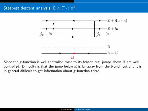
Since the g -function is well controlled close to its branch cut, jumps above R are wellcontrolled. Difficulty is that the jump below R is far away from the branch cut and it isin general difficult to get information about g -function there.
Since we have an explicit formula for gµ(z), we can just check
• For 0 ≤ µ < µc , jump on R− iδ is exponentially close to I.• For 0 < T < π2 and µ = µc +O(log(n)/n), jump is not small at the single pointz = −iδ. Local solution is given in terms of Hermite functions. Very similar to“birth of a cut” in random matrix models.
Karl Liechty NIBM on circle
Steepest descent analysis, 0 < T < π2
R
R + iµ
R + i(µ+ ε)
R− iδ
r r− 2√
T+ iµ 2√
T+ iµ
�
--
--
-
-
- -
6?
s−iδ
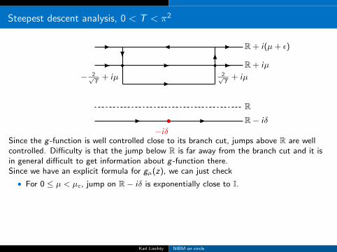
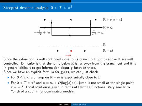
Since the g -function is well controlled close to its branch cut, jumps above R are wellcontrolled. Difficulty is that the jump below R is far away from the branch cut and it isin general difficult to get information about g -function there.Since we have an explicit formula for gµ(z), we can just check
• For 0 ≤ µ < µc , jump on R− iδ is exponentially close to I.
• For 0 < T < π2 and µ = µc +O(log(n)/n), jump is not small at the single pointz = −iδ. Local solution is given in terms of Hermite functions. Very similar to“birth of a cut” in random matrix models.
Karl Liechty NIBM on circle
Steepest descent analysis, 0 < T < π2
R
R + iµ
R + i(µ+ ε)
R− iδ
r r− 2√
T+ iµ 2√
T+ iµ
�
--
--
-
-
- -
6?
s−iδ
Since the g -function is well controlled close to its branch cut, jumps above R are wellcontrolled. Difficulty is that the jump below R is far away from the branch cut and it isin general difficult to get information about g -function there.Since we have an explicit formula for gµ(z), we can just check
• For 0 ≤ µ < µc , jump on R− iδ is exponentially close to I.• For 0 < T < π2 and µ = µc +O(log(n)/n), jump is not small at the single pointz = −iδ. Local solution is given in terms of Hermite functions. Very similar to“birth of a cut” in random matrix models.
Karl Liechty NIBM on circle
Steepest descent analysis: T ≈ π2
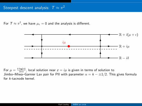
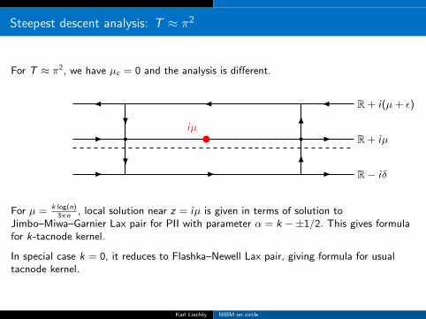
For T ≈ π2, we have µc = 0 and the analysis is different.
R + iµ
R + i(µ+ ε)
R− iδ
r r� ��
--
-- -
6?
? 6
uiµ
For µ = k log(n)3πn
, local solution near z = iµ is given in terms of solution toJimbo–Miwa–Garnier Lax pair for PII with parameter α = k −±1/2. This gives formulafor k-tacnode kernel.
In special case k = 0, it reduces to Flashka–Newell Lax pair, giving formula for usualtacnode kernel.
Karl Liechty NIBM on circle
Steepest descent analysis: T ≈ π2
For T ≈ π2, we have µc = 0 and the analysis is different.
R + iµ
R + i(µ+ ε)
R− iδ
r r� ��
--
-- -
6?
? 6
uiµ
For µ = k log(n)3πn
, local solution near z = iµ is given in terms of solution toJimbo–Miwa–Garnier Lax pair for PII with parameter α = k −±1/2. This gives formulafor k-tacnode kernel.
In special case k = 0, it reduces to Flashka–Newell Lax pair, giving formula for usualtacnode kernel.
Karl Liechty NIBM on circle
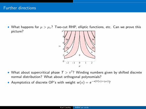
Further directions
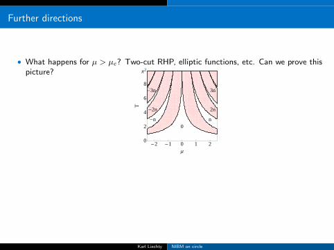
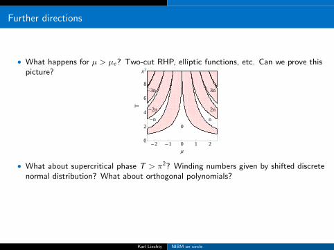
• What happens for µ > µc? Two-cut RHP, elliptic functions, etc. Can we prove thispicture?
0n-n
-2n 2n
3n-3n
-2 -1 0 1 20
2
4
6
8
Π2
Μ
T
• What about supercritical phase T > π2? Winding numbers given by shifted discretenormal distribution? What about orthogonal polynomials?
• Asymptotics of discrete OP’s with weight w(x) = e−n(V (x)+iµx)?
• More general discrete OP’s with complex weights?
Karl Liechty NIBM on circle
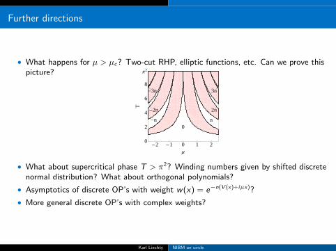
Further directions
• What happens for µ > µc? Two-cut RHP, elliptic functions, etc. Can we prove thispicture?
0n-n
-2n 2n
3n-3n
-2 -1 0 1 20
2
4
6
8
Π2
Μ
T
• What about supercritical phase T > π2? Winding numbers given by shifted discretenormal distribution? What about orthogonal polynomials?
• Asymptotics of discrete OP’s with weight w(x) = e−n(V (x)+iµx)?
• More general discrete OP’s with complex weights?
Karl Liechty NIBM on circle
References
• K. Liechty and D. Wang, Nonintersecting Brownian motions on the unit circle, Ann.Probab. 44, 1134–1211 (2016).
• R. Buckingham and K. Liechty, Nonintersecting Brownian bridges on the unit circlewith drift, arXiv:1707.07211 (2017).
• R. Buckingham and K. Liechty, The k-tacnode process, arXiv:1709......
Karl Liechty NIBM on circle
Thanks
Thanks!!
Karl Liechty NIBM on circle