kauai island utility co-op (kiuc) pv integration study€¦ · photovoltaics and distributed...
TRANSCRIPT
SANDIA REPORT SAND2011-7541 Unlimited Release Printed August 2011
Kauai Island Utility Co-op (KIUC) PV Integration Study Tom Mousseau, EnerNex Corporation Abraham Ellis, Sandia National Laboratories Prepared by Sandia National Laboratories Albuquerque, New Mexico 87185 and Livermore, California 94550 Sandia National Laboratories is a multi-program laboratory managed and operated by Sandia Corporation, a wholly owned subsidiary of Lockheed Martin Corporation, for the U.S. Department of Energy’s National Nuclear Security Administration under contract DE-AC04-94AL85000. Approved for public release; further dissemination unlimited.

2
Issued by Sandia National Laboratories, operated for the United States Department of Energy by Sandia Corporation. NOTICE: This report was prepared as an account of work sponsored by an agency of the United States Government. Neither the United States Government, nor any agency thereof, nor any of their employees, nor any of their contractors, subcontractors, or their employees, make any warranty, express or implied, or assume any legal liability or responsibility for the accuracy, completeness, or usefulness of any information, apparatus, product, or process disclosed, or represent that its use would not infringe privately owned rights. Reference herein to any specific commercial product, process, or service by trade name, trademark, manufacturer, or otherwise, does not necessarily constitute or imply its endorsement, recommendation, or favoring by the United States Government, any agency thereof, or any of their contractors or subcontractors. The views and opinions expressed herein do not necessarily state or reflect those of the United States Government, any agency thereof, or any of their contractors. Printed in the United States of America. This report has been reproduced directly from the best available copy. Available to DOE and DOE contractors from U.S. Department of Energy Office of Scientific and Technical Information P.O. Box 62 Oak Ridge, TN 37831 Telephone: (865) 576-8401 Facsimile: (865) 576-5728 E-Mail: [email protected] Online ordering: http://www.osti.gov/bridge Available to the public from U.S. Department of Commerce National Technical Information Service 5285 Port Royal Rd. Springfield, VA 22161 Telephone: (800) 553-6847 Facsimile: (703) 605-6900 E-Mail: [email protected] Online order: http://www.ntis.gov/help/ordermethods.asp?loc=7-4-0#online
3
SAND2011-7541 Unlimited Release
Printed August 2011
Kauai Island Utility Co-op (KIUC) PV Integration Study
Abraham Ellis Photovoltaics and Distributed Systems Integration
Sandia National Laboratories P.O. Box 5800
Albuquerque, New Mexico 87185-1033
Tom Mousseau 620 Mabry Hood Road, Suite 300
Knoxville, TN 37922
Abstract
This report investigates the effects that increased distributed photovoltaic (PV) generation would have on the Kauai Island Utility Co-op (KIUC) system operating requirements. The study focused on determining reserve requirements needed to mitigate the impact of PV variability on system frequency, and the impact on operating costs. Scenarios of 5-MW, 10-MW, and 15-MW nameplate capacity of PV generation plants distributed across the Kauai Island were considered in this study. The analysis required synthesis of the PV solar resource data and modeling of the KIUC system inertia. Based on the results, some findings and conclusions could be drawn, including that the selection of units identified as marginal resources that are used for load following will change; PV penetration will displace energy generated by existing conventional units, thus reducing overall fuel consumption; PV penetration at any deployment level is not likely to reduce system peak load; and increasing PV penetration has little effect on load-following reserves. The study was performed by EnerNex under contract from Sandia National Laboratories with cooperation from KIUC.

4

5
Contents
Executive Summary .......................................................................................................................11
1 Introduction ..............................................................................................................................15 1.1 Introduction .....................................................................................................................15 1.2 Scope ...............................................................................................................................15 1.3 Requirements ..................................................................................................................16
2 Project Assumptions ................................................................................................................17 2.1 Data Availability .............................................................................................................17
2.1.1 KIUC Data .........................................................................................................17 2.1.2 NREL Solar Data ...............................................................................................18
2.2 Conversion from Irradiance to Power Output .................................................................21 2.3 Other Assumptions..........................................................................................................22
3 Study Scenario .........................................................................................................................23 3.1 Scenario Description .......................................................................................................23 3.2 PV Data Modeling ..........................................................................................................23
3.2.1 Year-to-Year Comparison .................................................................................25 3.2.2 Analysis of Selected Sites .................................................................................31 3.2.3 Correlation of Selected Sites .............................................................................32 3.2.4 Correlation Data of High-Resolution Data ........................................................33
3.3 Scenario Analysis............................................................................................................35 3.3.1 Capacity Factor and Energy from Solar ............................................................35 3.3.2 PV Duration .......................................................................................................37 3.3.3 Net Load Duration .............................................................................................39
4 Methodology ............................................................................................................................41 4.1 KIUC System Model.......................................................................................................41
4.1.1 System Model ....................................................................................................42 4.1.2 System Simulation of Base Case .......................................................................43 4.1.3 System Simulation with PV ..............................................................................47
4.2 Marginal Unit Identification ...........................................................................................51 4.3 Regulation Change Estimation .......................................................................................53
5 Analysis....................................................................................................................................55 5.1 Load Analysis .................................................................................................................55 5.2 Load Net PV Analysis ....................................................................................................57 5.3 Integration Analysis ........................................................................................................62
5.3.1 Marginal Units ...................................................................................................62 5.3.2 Regulation Increase ...........................................................................................63
6 Conclusions and Findings ........................................................................................................65
Appendix A. ...................................................................................................................................67
6
Figures Figure ES-1. On-line spinning capacity requirement to meet 99.7% of 15-second changes in
net load for study scenarios................................................................................................12 Figure 1. KUIC generation mix for 2011......................................................................................18 Figure 2. Sample of NREL 2005 Lihue Airport solar resource data. ...........................................19 Figure 3. Comparison of 1-second and 60-minute average Global Horizontal irradiance for
HECO Campbell on August 22, 2009................................................................................20 Figure 4. Cumulative probability distribution function of the absolute value of 1-second
ramp rates for Oahu data. ...................................................................................................21 Figure 5. Map of site locations. ....................................................................................................24 Figure 6. Monthly solar resource data at Lihue Airport, 2000–2005. ..........................................25 Figure 7. Annual solar resource data at Lihue Airport, 2000–2005. ............................................26 Figure 8. Monthly solar resource data at Honolulu Airport, 2000–2005. .....................................26 Figure 9. Annual solar resource data at Honolulu Airport, 2000–2005. .......................................27 Figure 10. Monthly solar resource data at Kahului Airport, 2000–2005. .....................................27 Figure 11. Annual solar resource data at Kahului Airport, 2000–2005. .......................................28 Figure 12. Monthly solar resource data at Hilo International Airport, 2000–2005. .....................28 Figure 13. Annual solar resource data at Hilo International Airport, 2000–2005. .......................29 Figure 14. Selected sites and solar data representation.................................................................30 Figure 15. Monthly solar resource data at selected sites. .............................................................31 Figure 16. Average monthly and annual solar resource data statistics for Site 1. ........................31 Figure 17. Cumulative distribution function of selected sites. .....................................................32 Figure 18. Total monthly energy from solar PV for each scenario. .............................................36 Figure 19. Annual energy as a percent of load energy. ................................................................37 Figure 20. PV duration for scenarios. ...........................................................................................38 Figure 21. PV penetration for scenarios. ......................................................................................38 Figure 22. Load net PV duration curve for scenarios. ..................................................................39 Figure 23. PV generation effect on peak and minimum load. ......................................................40 Figure 24. PV generation effect on peak and minimum load – zoomed. ......................................40 Figure 25. Block diagram of used system model with supplementary control. ............................43 Figure 26. Load profile for a one-day period. ...............................................................................44 Figure 27. System frequency profile for a one-day period. ..........................................................44 Figure 28. 15-second time-scale load variability. .........................................................................45 Figure 29. 15-second time-scale generation variability. ...............................................................45 Figure 30. Simulated and measured (provided by KIUC) system frequency. ..............................46 Figure 31. Measured and simulated frequency for sample hour. ..................................................46 Figure 32. Load and load net PV 15-second profile for a one-day period. ...................................47 Figure 33. 15-second time-scale load and load net PV variability. ..............................................48 Figure 34. Simulated system frequency without additional regulation. .......................................49 Figure 35. Required power plant output variability. .....................................................................49 Figure 36. Simulated system frequency with additional regulation. ............................................50 Figure 37. Load duration curve with marginal unit distribution. ..................................................52 Figure 38. Monthly occurrence of identified marginal units. .......................................................52 Figure 39. Scenario 3 sub-hourly load net PV variability. ...........................................................54 Figure 40. Sub-hourly load variability with no PV.......................................................................54
7
Figure 41. Average daily load shape for each month. ..................................................................55 Figure 42. Monthly minimum and maximum load for study period. ...........................................56 Figure 43. Monthly load energy for the study period. ..................................................................56 Figure 44. Load duration curve of monthly load and load net PV variations for one month. ......58 Figure 45. Load duration curve of load and load net PV 15-second variations for one day
(5760 data samples). ..........................................................................................................58 Figure 46. Histogram of load and load net PV hourly variations for one month. ........................59 Figure 47. Histogram of load and load net PV 15-second variations for one day. .......................60 Figure 48. PV generation variability over load generation level. .................................................62 Figure 49. Monthly marginal units cost. .......................................................................................62 Figure 50. On-line spinning capacity requirement to meet 99.7% of 15-second changes in net
load for study scenarios. ....................................................................................................65
Tables Table ES-1. Annual Incremental Reserve Range. ........................................................................13 Table 1. 1-Second Ramp Rate Statistics for Daytime Irradiance Change Oahu Data. .................20 Table 2. PV Central Systems Distribution and Capacity for Three Scenarios. ............................23 Table 3. Site Locations. ................................................................................................................24 Table 4. Solar Resource Data Correlation Coefficient in December for Selected Sites. ..............33 Table 5. Correlation Coefficient of Average Hourly Solar Resource Data for Sites at Oahu
on August 22, 2009. ...........................................................................................................33 Table 6. Correlation Coefficient of 1–Second Solar Resource Data for Oahu Data on August
22, 2009..............................................................................................................................34 Table 7. Correlation Coefficients of 1–Second Irradiance for Selected Sites on December 9. ....34 Table 8. Summary of Capacity, Capacity Factor, and Annual Energy by Sites for Scenario 1. ..35 Table 9. Summary of Capacity, Capacity Factor, and Annual Energy by Sites for Scenario 2. ..35 Table 10. Summary of Capacity, Capacity Factor, and Annual Energy by Sites for Scenario
3..........................................................................................................................................36 Table 11. Summary of 15-Second Generation Change Showing Maximum (Hi) and
Minimum (Lo) Up-Ramp (Positive Variability) and Maximum (Lo) and Minimum (Hi) Down-Ramp (Negative Variability in MW for the Month of December. ..................50
Table 12. Summary of Monthly Load and Energy for the Study Period. .....................................57 Table 13. Load-Following Reserve Assumption for May Based on the 99.7th Percentile
Coverage. ...........................................................................................................................61 Table 14. Incremental Reserve Assumption Based on the 99.7th Percentile Coverage. ...............61 Table 15. Percent Reduction in Marginal Unit Costs for Each Scenario in March and July. .......63 Table 16. Annual Percent Reduction in Marginal Unit Cost. .......................................................63 Table 17. Additional Regulation Energy Required for Each Day Based on Unit 15-Second
Variability. .........................................................................................................................64 Table 18. Average Daily Additional Regulation for the Month of December. ............................64 Table 19. Annual Incremental Reserve Range. ............................................................................66

8

9
Acronyms AGC Automatic Generation Control DOE Department of Energy ETR Extraterrestrial Radiation ETRN Extraterrestrial Normal Radiation HCEI Hawaii Clean Energy Initiative HECO Hawaiian Electric Company KIUC Kauai Island Utility Co-op METSTAT Dir Meteorological Statistical Model Direct Normal NREL National Renewable Energy Laboratory PV photovoltaic SNL Sandia National Laboratories SUNY Glo Global Solar Radiation SUNY State University of New York

10
11
Executive Summary
ES-1 Overview This report investigates the effects that increased distributed photovoltaic (PV) generation would have on the Kauai Island Utility Co-op (KIUC) system operating requirements. The study focused on determining reserve requirements needed to mitigate the impact of PV variability on system frequency. The analysis was performed by examining the impact on system frequency and operating costs. Scenarios of 5-MW, 10-MW and 15-MW nameplate capacity of PV generation plants distributed across the Kauai Island were considered in this study. The study was performed by EnerNex under contract from Sandia National Laboratories with cooperation from KIUC. ES-2 Approach The study collected solar resource data and system operation data from readily available sources. Hourly solar resource data was acquired from the National Renewable Energy Laboratory solar database for years 2000–2005. Higher-resolution solar data provided by KIUC consisting of data for partial years was used to develop profiles and statistical representations of data. The statistical characterization of this data was applied to the NREL solar resource data to model intra-hour variability. In addition, KIUC provided a description of their operating system with UPLAN data depicting generation operation, operation costs, and projected load growth. KIUC also supplied high-resolution (15-second) system frequency data for December 1–21, 2009. A system model was created, using the block diagram language VisSim, to mimic the KIUC system. KIUC provided data consisting of generation output, system load, and system frequency. The model input was generation and system load. The model output was system frequency response. A Base Case was defined that used the KIUC system generation output and system load. The model was tuned such that the output frequency response would closely match the provided KIUC system frequency. Using the tuned model, a scenario of distributed PV generation was added to the Base Case configuration. The resulting output of frequency from the model showed degradation in system frequency. The model was tuned to the KIUC system frequency by adding regulating reserve capacity. The amount of generation output modification was captured and analyzed to demonstrate the PV effects on the system. KIUC provided UPLAN data that was used to approximate system production costs for the study period (2011) and to estimate the overall impact of the different PV penetration scenarios on system operations. The regulation reserve requirements established in the previous step were applied to the UPLAN production cost simulations.
12
ES-3 Findings and Conclusions Through the analysis of the PV solar resource data and the modeling of the KIUC system with 5-MW, 10-MW, and 15-MW nameplate capacity of PV generation, the following findings and conclusions can be drawn:
• The selection of units identified as marginal resources that serve and follow system load will change. As PV generation increases, units identified as marginal resources will be units with lower operating costs. In general the cost of operations for marginal units will be reduced.
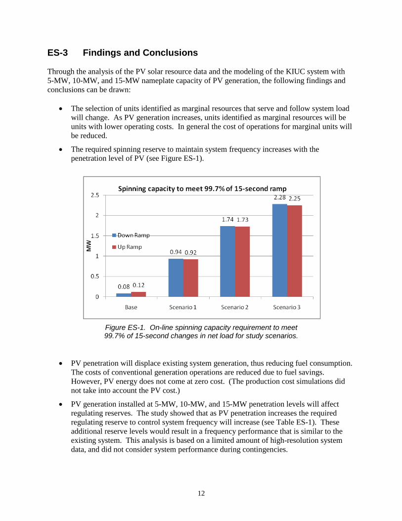
• The required spinning reserve to maintain system frequency increases with the penetration level of PV (see Figure ES-1).
Figure ES-1. On-line spinning capacity requirement to meet 99.7% of 15-second changes in net load for study scenarios.
• PV penetration will displace existing system generation, thus reducing fuel consumption. The costs of conventional generation operations are reduced due to fuel savings. However, PV energy does not come at zero cost. (The production cost simulations did not take into account the PV cost.)
• PV generation installed at 5-MW, 10-MW, and 15-MW penetration levels will affect regulating reserves. The study showed that as PV penetration increases the required regulating reserve to control system frequency will increase (see Table ES-1). These additional reserve levels would result in a frequency performance that is similar to the existing system. This analysis is based on a limited amount of high-resolution system data, and did not consider system performance during contingencies.
13
• PV penetration at any penetration level is not likely to reduce system peak load. KIUC load patterns peak in the evening with a secondary peak in the morning. The peaks occur at times when PV generation is at low or zero level. PV has the best benefit for reducing system peak in the summer months when the solar day is longer.
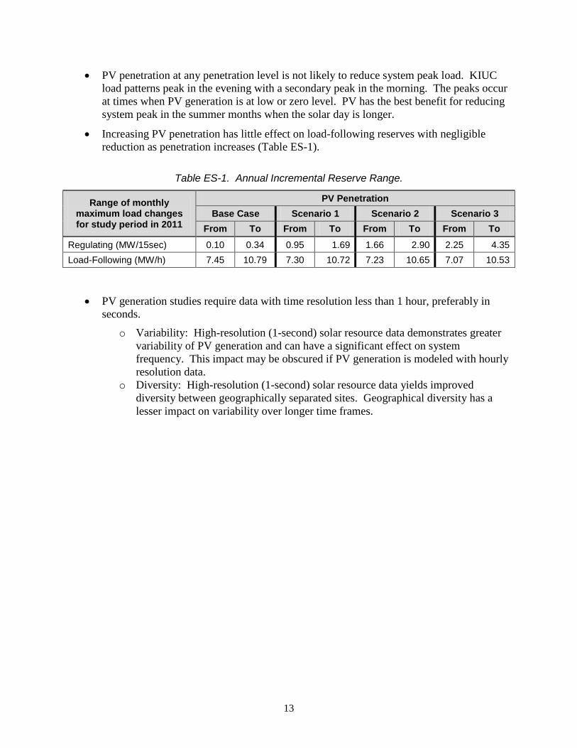
• Increasing PV penetration has little effect on load-following reserves with negligible reduction as penetration increases (Table ES-1).
Table ES-1. Annual Incremental Reserve Range.
Range of monthly maximum load changes for study period in 2011
PV Penetration Base Case Scenario 1 Scenario 2 Scenario 3
From To From To From To From To Regulating (MW/15sec) 0.10 0.34 0.95 1.69 1.66 2.90 2.25 4.35 Load-Following (MW/h) 7.45 10.79 7.30 10.72 7.23 10.65 7.07 10.53
• PV generation studies require data with time resolution less than 1 hour, preferably in seconds.
o Variability: High-resolution (1-second) solar resource data demonstrates greater variability of PV generation and can have a significant effect on system frequency. This impact may be obscured if PV generation is modeled with hourly resolution data.
o Diversity: High-resolution (1-second) solar resource data yields improved diversity between geographically separated sites. Geographical diversity has a lesser impact on variability over longer time frames.

14
15
1 Introduction
1.1 Introduction This report describes the potential effect of introducing different penetration levels of photovoltaic (PV) power into the Kauai Island Utility Co-op (KIUC) power system. The analysis was performed by EnerNex under contract to Sandia National Laboratories (SNL), and funded by the U.S Department of Energy (DOE). In January 2008 the Hawaiian governor signed a Memorandum of Understanding with DOE to the Hawaiian-DOE Clean Energy Initiative (HCEI). This was an unprecedented effort to transform the entire Hawaii economy from receiving 95% of its energy, including most electricity, from imported oil today, to meeting the state's energy needs with 70% clean energy (primarily indigenous renewables and efficiency) by 2030. To assist in meeting the goals of the HCEI, the KIUC is developing a renewable energy roadmap for the Hawaiian Island of Kauai. In providing support of the roadmap development, SNL has been tasked to supply KIUC with a preliminary solar integration impact study for the Kauai Island. EnerNex was contracted to work with SNL to assist in completing this task. This report provides description of the effort and its findings. 1.2 Scope The scope of this study is to estimate potential operational and cost impacts of increasingly higher penetration of PV output on the KIUC system. The study relied upon the use of well-established tools and methodologies that have been used in the analysis of renewable resource integration studies for larger systems. Additional revisions to these methodologies were made to deal with the microgrid setting and higher time resolution needed to capture short-term PV power output impacts. Early in the project it was determined the study would examine the impact of three scenarios of various PV integration. The first scenario totaling 5 MW of nameplate generation consists of one 3-MW and two 1-MW PV plants. The second scenario provides 10 MW of nameplate generation consisting of two 3-MW and four 1-MW plants. The third scenario consists of 15 MW of nameplate generation with four 3-MW and three 1-MW plants. This report provides details and analysis of data for each of the scenarios. As an intermediate step in this study, there was an examination of the effect of PV on reserve requirements to maintain system reliability. To examine high-resolution time-domain simulations of the KIUC system, a commercially available modeling tool, VisSim, was used to take into account the impact of KIUC’s Automatic Generation Control (AGC) system. It is not in the scope of this project to evaluate auxiliary costs of PV implementation such as the cost of construction, transmission and distribution lines, capital cost of plants, licensing, regulatory costs, permit costs, location siting, and PV integration or compatibility with the
16
current KIUC generation system. For the purpose of the study the PV siting does not map to specific locations on the Kauai Island, nor is it the intent of this report to propose construction locations of PV sites on the island. 1.3 Requirements An important aspect of the study involves the collection and identification of useful and accurate data from which results, analysis, findings, and recommendations are derived. The National Renewable Energy Laboratory (NREL) has several years of measured solar resource data for different sites on the Hawaiian Islands. One site from the database was on the Kauai Island at the Lihue airport. This was the only site for Kauai in the NREL database. To this end the project team identified early on that long range (year or more) periodically continuous solar resource PV data was limited to a single site on the island. To incorporate diversity into the analysis, the NREL database provided solar resource data for other locations on the Hawaiian Islands. These locations were examined statistically and used in the study. In addition, KIUC provided measured solar data from various sites on the different islands. This data consisted of assorted time resolution PV data for different time periods less than a year in duration. A method for estimating solar plant output based on the irradiance data was provided by SNL. Details of the PV data used for the study can be found in Section 2.1. Understanding the KIUC system and its response to large amounts of PV capacity penetration required building a model of the KIUC system including the effects of inertia and AGC. The KIUC system model representing in its present state with 3 MW of distributed PV penetration (Base Case) was validated and used as an operations baseline. Additional scenarios of the KIUC system for each PV penetration were analyzed for comparison against the Base Case. KIUC provided UPLAN data for 2010 that was used in the study as a representative model of the KIUC generation system. The data consisted of generation resource configurations and system loads and was used as input for the system model. The UPLAN model allows for estimation of production cost and assessment of generation adequacy. The study year was selected to be 2011. Load data for 2011 was derived by escalating the 2010 UPLAN load data at 1%. There were no generation fleet additions or retirements between 2010 and 2011.
17
2 Project Assumptions
2.1 Data Availability
2.1.1 KIUC Data The data provided by KIUC consisted of generation information for supply, load data for demand, and selected PV metered data at different resolution and duration. The list of the received data included:
• KIUC Hourly – 2006 loads – grown from 2004/2005 actual load
• KIUC 15-second frequency 12/1/09 – 12/21/09
• KIUC 15-minute system load 2005, 2008, 2009
• KIUC Warehouse PV Project 1-second real power 5/27/10 – 6/22/10
• Ahukini PV Project 1-second real power 2/23/10 – 3/11/10, 5/20/10 – 5/27/10, 5/27/10 – 6/9/10, 5/27/10 – 6/14/10
• Koloa Sub T21 2-second frequency data 7/14/10 – 7/16/10, 7/14/10 – 7/19/10, 7/16/10 – 7/23/10, 7/23/10 – 7/30/10, 8/3/10 – 8/10/10
• Oahu 1-second normalized solar data (3 stations) 8/22/09 6 a.m. – 11:35 p.m.
• KIUC system data from UPLAN (input and output)
• Hana Kukui 2.5-minute solar irradiance 6/30/09 – 7/24/09
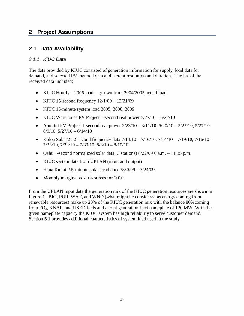
• Monthly marginal cost resources for 2010 From the UPLAN input data the generation mix of the KIUC generation resources are shown in Figure 1. BIO, PUR, WAT, and WND (what might be considered as energy coming from renewable resources) make up 20% of the KIUC generation mix with the balance 80%coming from FO2, KNAP, and USED fuels and a total generation fleet nameplate of 120 MW. With the given nameplate capacity the KIUC system has high reliability to serve customer demand. Section 5.1 provides additional characteristics of system load used in the study.
18
Figure 1. KUIC generation mix for 2011.
2.1.2 NREL Solar Data The NREL National Solar Radiation Database was a primary source of solar resource data for the study. The database provided a single source of solar resource data for the island of Kauai representative of the Lihue airport. To consider the effects of geographical diversity on the performance of large PV systems it was decided to select additional sites from the NREL database representing other Hawaiian islands. Using solar patterns consistent with solar resource data on the Hawaiian Islands yet different enough to allow various PV plant output was intended to provide a degree of diversity for the study. It was assumed that the statistical correlation of hourly solar resource data among the selected sites would be reasonably similar to sites within the island of Kauai.
8%
58%
18%
5% 4%
5%
2% KIUC Generation Mix 2011
BIO
FO2
KNAP
PUR
USED
WAT
WND
19
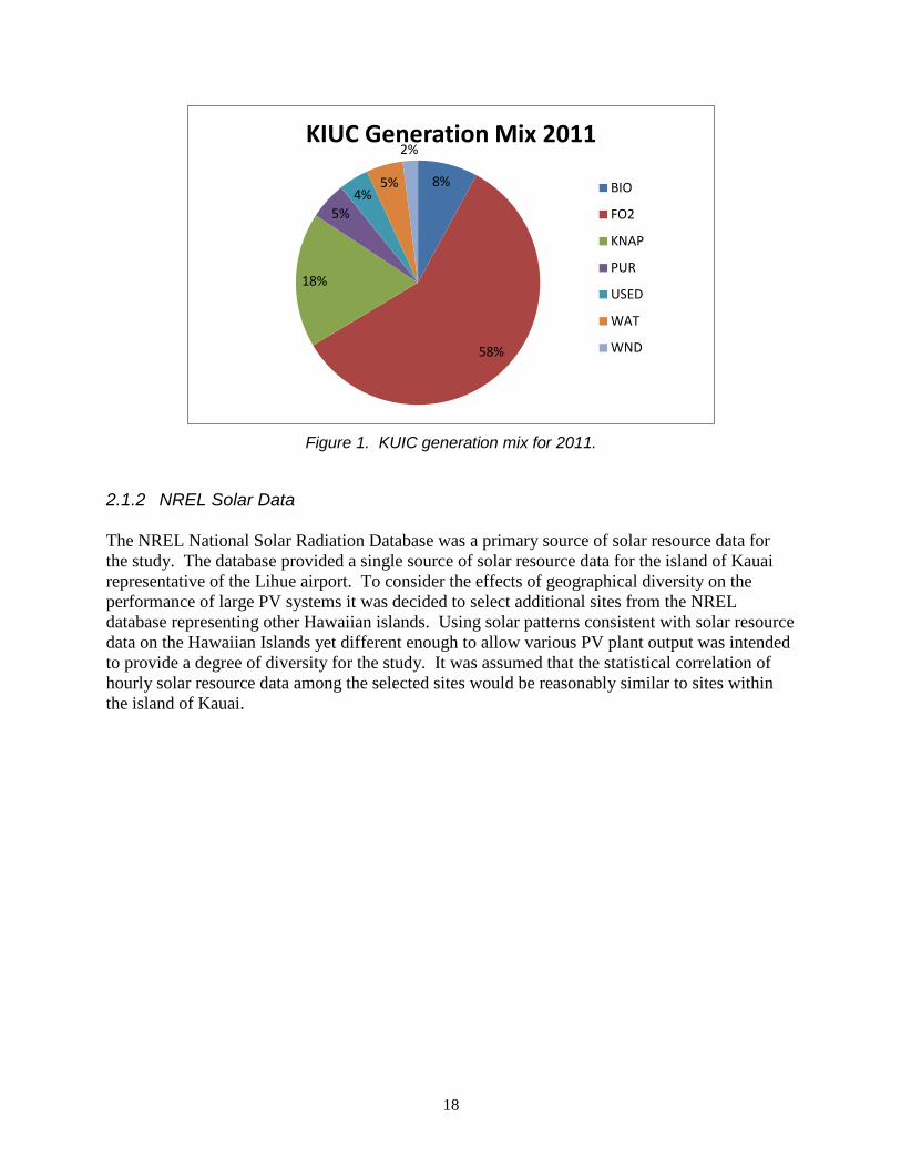
A sample of the NREL data from the Lihue airport is shown in Figure 2. The database includes four measurements of solar resource data:
• ETR: Extraterrestrial Radiation
• ETRN: Extraterrestrial Normal Radiation
• SUNY Glo: Global Solar Radiation
• METSTAT Dir: Meteorological Statistical Model Direct Normal
Figure 2. Sample of NREL 2005 Lihue Airport solar resource data.
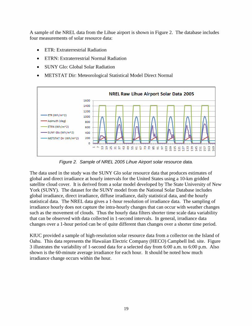
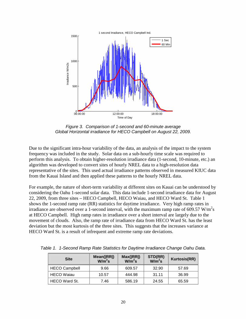
The data used in the study was the SUNY Glo solar resource data that produces estimates of global and direct irradiance at hourly intervals for the United States using a 10-km gridded satellite cloud cover. It is derived from a solar model developed by The State University of New York (SUNY). The dataset for the SUNY model from the National Solar Database includes global irradiance, direct irradiance, diffuse irradiance, daily statistical data, and the hourly statistical data. The NREL data gives a 1-hour resolution of irradiance data. The sampling of irradiance hourly does not capture the intra-hourly changes that can occur with weather changes such as the movement of clouds. Thus the hourly data filters shorter time scale data variability that can be observed with data collected in 1-second intervals. In general, irradiance data changes over a 1-hour period can be of quite different than changes over a shorter time period. KIUC provided a sample of high-resolution solar resource data from a collector on the Island of Oahu. This data represents the Hawaiian Electric Company (HECO) Campbell Ind. site. Figure 3 illustrates the variability of 1-second data for a selected day from 6:00 a.m. to 6:00 p.m. Also shown is the 60-minute average irradiance for each hour. It should be noted how much irradiance change occurs within the hour.
20
Figure 3. Comparison of 1-second and 60-minute average
Global Horizontal irradiance for HECO Campbell on August 22, 2009. Due to the significant intra-hour variability of the data, an analysis of the impact to the system frequency was included in the study. Solar data on a sub-hourly time scale was required to perform this analysis. To obtain higher-resolution irradiance data (1-second, 10-minute, etc.) an algorithm was developed to convert sites of hourly NREL data to a high-resolution data representative of the sites. This used actual irradiance patterns observed in measured KIUC data from the Kauai Island and then applied these patterns to the hourly NREL data. For example, the nature of short-term variability at different sites on Kauai can be understood by considering the Oahu 1-second solar data. This data include 1-second irradiance data for August 22, 2009, from three sites – HECO Campbell, HECO Waiau, and HECO Ward St. Table 1 shows the 1-second ramp rate (RR) statistics for daytime irradiance. Very high ramp rates in irradiance are observed over a 1-second interval, with the maximum ramp rate of 609.57 W/m2s at HECO Campbell. High ramp rates in irradiance over a short interval are largely due to the movement of clouds. Also, the ramp rate of irradiance data from HECO Ward St. has the least deviation but the most kurtosis of the three sites. This suggests that the increases variance at HECO Ward St. is a result of infrequent and extreme ramp rate deviations.
Table 1. 1-Second Ramp Rate Statistics for Daytime Irradiance Change Oahu Data.
Site Mean(|RR|) W/m2s
Max(|RR|) W/m2s
STD(RR) W/m2s Kurtosis(RR)
HECO Campbell 9.66 609.57 32.90 57.69 HECO Waiau 10.57 444.98 31.11 36.99 HECO Ward St. 7.46 586.19 24.55 65.59
06:00:00 12:00:00 18:00:000
500
1000
1500
Time of Day
Irrad
ianc
e W
/m2s
1 second Irradiance, HECO Campbell Ind.
1 Sec60 Min

21
The cumulative probability distribution of the absolute value of the ramp rates for each site is shown in Figure 4. This represents the probability of the ramp rate occurring. The dotted line marks the 95th percentile of the ramp rates observed for each sites. From the chart, it can be interpreted that there is only a 5% chance that the ramp rate at HECO Waiau, HECO Campbell, and HECO Ward St. will be larger than 40 W/m2, 55 W/m2, and 60 W/m2 respectively.
Figure 4. Cumulative probability distribution function
of the absolute value of 1-second ramp rates for Oahu data. To account for short-term variability in irradiance, the short-term variability pattern observed from the data provided by KIUC was mapped on the hourly average radiation data obtained from NREL database. It is necessary to account for the ramp rates because the majority of the variability in the PV power output is a result of variability in irradiance throughout the day. 2.2 Conversion from Irradiance to Power Output The irradiance data provided by KIUC represents a single-sensor irradiance measurement; therefore, simply scaling up the single-sensor irradiance will result in exaggerated ramp rates of the actual PV plants. From previous studies, it is observed that the total energy flux of a PV plant can be calculated as a simple moving time average of the single-point irradiance output, where the averaging time is related to the dimensions of the solar field or size of the PV plant and to the cloud speed.1 To account for the large solar fields and PV plant size modeled in this study, the irradiance data is processed as follows to approximate 95th percentile of short-term ramps:
• 1-MW systems: 20-second running average of single-sensor measurements
• 3-MW systems: 30-second running average of single-sensor measurements
1 A. Longhetto et al., Effect of correlations in time and spatial extent on performance of very large solar conversion
systems, Solar Energy, Vol. 43, No 2, pp. 77-84, 1989.

22
The delay parameters were provided by SNL based on analysis of PV irradiance and power output at the Lanai PV system and other sites. In a general sense, the delay parameters are related to cloud velocity, which should be similar in Kauai. The above approximation is based on the assumption that the plant output is the spatial average of irradiance over PV array footprint. In reality, the time average window that results in matching the 95th percentile of ramps is a function of wind speed, which varies constantly. However, the approximations of the 1-MW and 3-MW systems give a good representation of the output characteristics of large PV systems. A simple efficiency PV model was used to convert irradiance data to output power. The irradiance conversion model used a single, constant derate factor of 0.85 when converting solar energy from DC to AC electricity. The derate factor accounts for module mismatch, DC wiring losses, AC wiring losses, soiling, inverter efficiency, and inaccuracy in the PV module AC nameplate rating. 2.3 Other Assumptions Assumptions made in this study are listed below:
• 1- and 3-MW plant sizes were used in this study. The required area and specific locations of the plants were assumed available and feasible to tie into the existing KIUC electric system.
• The PV generated will be a must take form of generation. System load will be adjusted by the amount of generation output provided by the PV plant.
• Plant sizes assumed for each scenario are assumed to be net AC output rating.
• PV plants are assumed to be flat plate PV, fixed axis, and southern azimuth.
• KIUC stated the impact of existing 3 MW of distributed PV generation has not been of concern to their operations dispatch because the PV generation is dispersed and short-term variability is mitigated. For this reason the base case for the analysis included the frequency effects caused by existing distributed PV generation.
• PV forecast data does not exist for equivalent actual PV generation. For this study, PV forecast error was assumed to be a persistence forecast.
• In the time frame of 2010 to 2011 there are no retirements or additions to the KIUC generation fleet. All generation performance, operating dispatch practices, and fuel costs are assumed same as in 2009 to 2010. From these assumptions it is concluded that the costs for operating the generation fleet in 2010 would be the same in 2011 if the system load in 2011 was identical to 2010.
• KIUC operates as an island system without interconnection to neighboring utilities. In this study only KIUC generation and loads will be modeled. The modeling of transmission is not considered necessary for this analysis.
23
3 Study Scenario
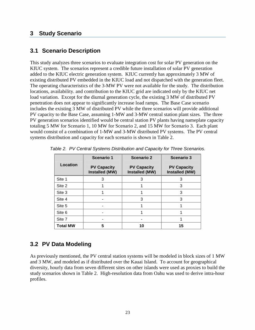
3.1 Scenario Description This study analyzes three scenarios to evaluate integration cost for solar PV generation on the KIUC system. The scenarios represent a credible future installation of solar PV generation added to the KIUC electric generation system. KIUC currently has approximately 3 MW of existing distributed PV embedded in the KIUC load and not dispatched with the generation fleet. The operating characteristics of the 3-MW PV were not available for the study. The distribution locations, availability. and contribution to the KIUC grid are indicated only by the KIUC net load variation. Except for the diurnal generation cycle, the existing 3 MW of distributed PV penetration does not appear to significantly increase load ramps. The Base Case scenario includes the existing 3 MW of distributed PV while the three scenarios will provide additional PV capacity to the Base Case, assuming 1-MW and 3-MW central station plant sizes. The three PV generation scenarios identified would be central station PV plants having nameplate capacity totaling 5 MW for Scenario 1, 10 MW for Scenario 2, and 15 MW for Scenario 3. Each plant would consist of a combination of 1-MW and 3-MW distributed PV systems. The PV central systems distribution and capacity for each scenario is shown in Table 2.
Table 2. PV Central Systems Distribution and Capacity for Three Scenarios.
Location Scenario 1
PV Capacity
Installed (MW)
Scenario 2
PV Capacity Installed (MW)
Scenario 3
PV Capacity Installed (MW)
Site 1 3 3 3 Site 2 1 1 3 Site 3 1 1 3 Site 4 - 3 3 Site 5 - 1 1 Site 6 - 1 1 Site 7 - - 1 Total MW 5 10 15
3.2 PV Data Modeling As previously mentioned, the PV central station systems will be modeled in block sizes of 1 MW and 3 MW, and modeled as if distributed over the Kauai Island. To account for geographical diversity, hourly data from seven different sites on other islands were used as proxies to build the study scenarios shown in Table 2. High-resolution data from Oahu was used to derive intra-hour profiles.
24
Some of the considerations for proxy site selection include:
• The solar resource data at selected sites must be a close representation of the solar resource data patterns observed throughout the year on Kauai Island.
• The availability of a single site of solar resource data on Kauai correlated with the solar resource data at the selected sites. The need for selection of the other island solar resource data is recognized as being a less than conservative assumption; however, this solar resource data provided diversity at the intra-hour level.
• Sites selected should provide adequate spatial and temporal diversity in irradiance and hence diversity in the power generated at the sites for the different scenarios under consideration.
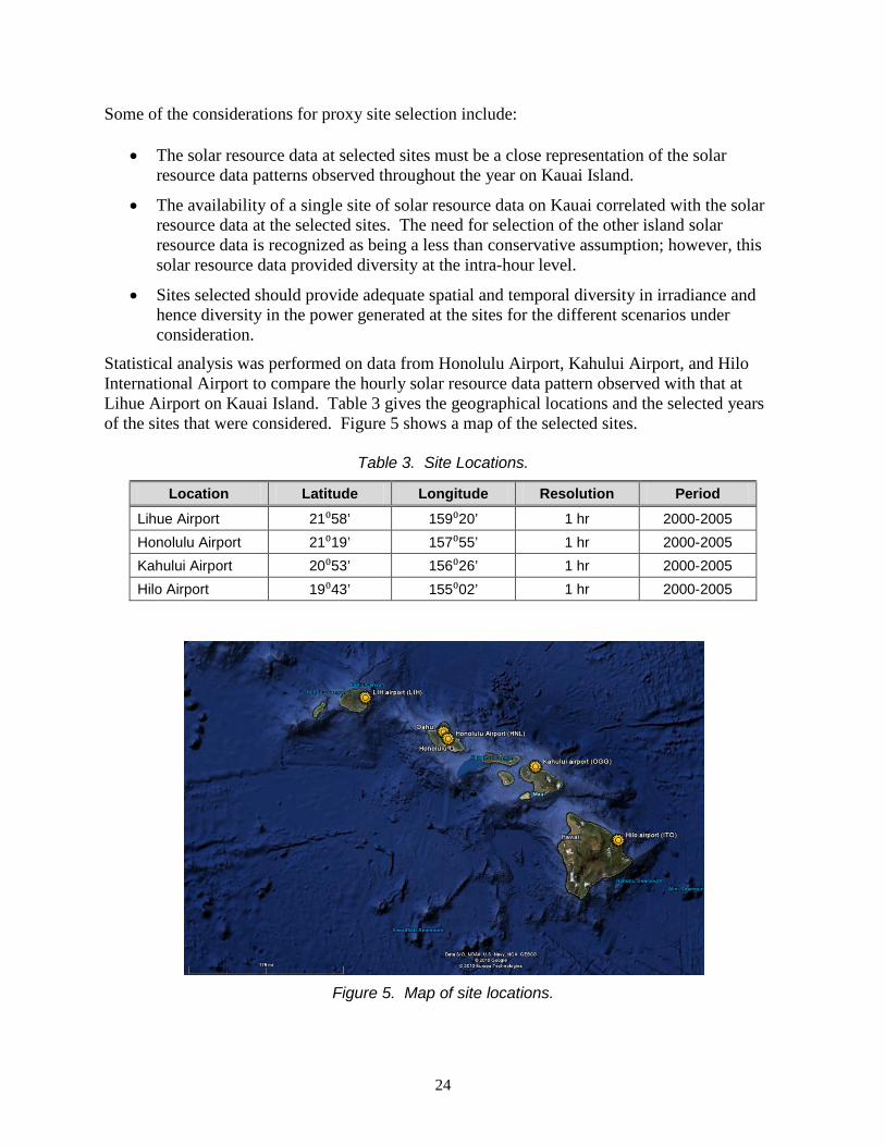
Statistical analysis was performed on data from Honolulu Airport, Kahului Airport, and Hilo International Airport to compare the hourly solar resource data pattern observed with that at Lihue Airport on Kauai Island. Table 3 gives the geographical locations and the selected years of the sites that were considered. Figure 5 shows a map of the selected sites.
Table 3. Site Locations.
Location Latitude Longitude Resolution Period
Lihue Airport 21⁰58’ 159⁰20’ 1 hr 2000-2005 Honolulu Airport 21⁰19’ 157⁰55’ 1 hr 2000-2005 Kahului Airport 20⁰53’ 156⁰26’ 1 hr 2000-2005 Hilo Airport 19⁰43’ 155⁰02’ 1 hr 2000-2005
Figure 5. Map of site locations.
25
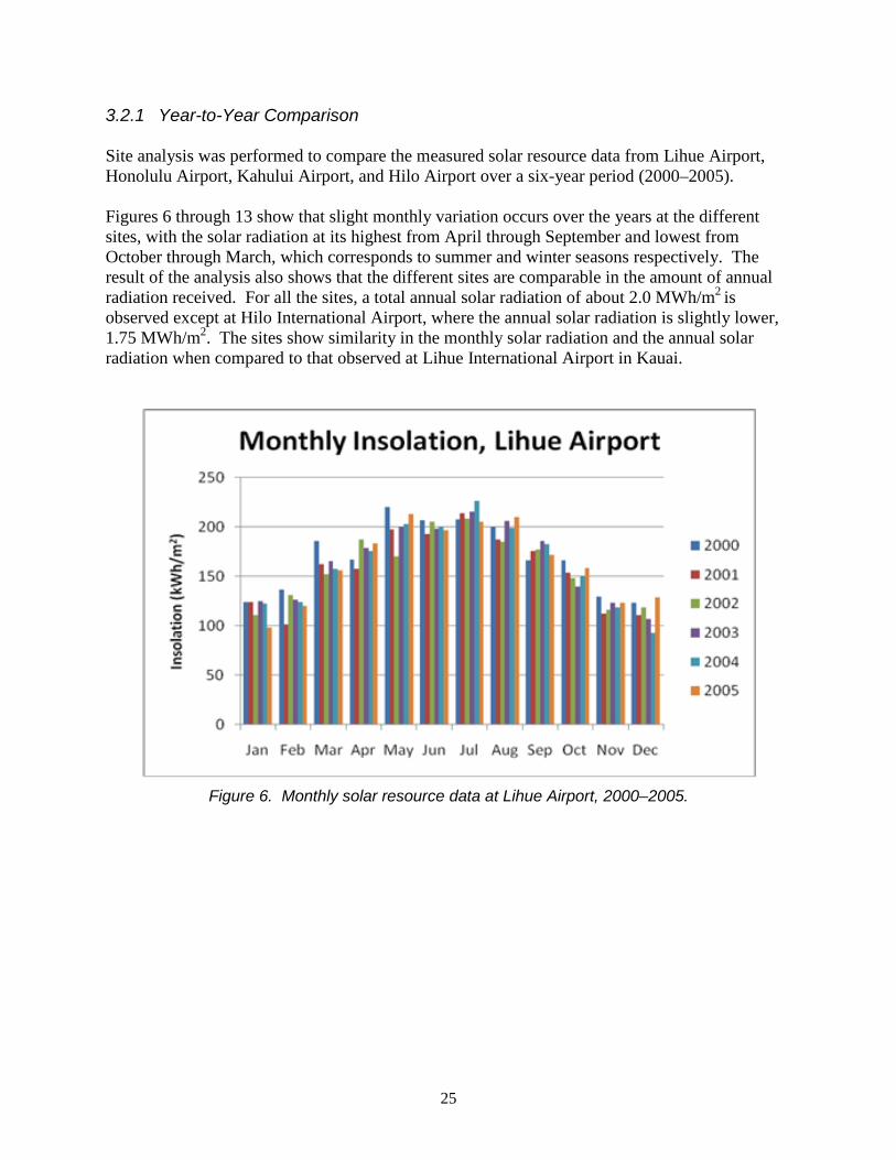
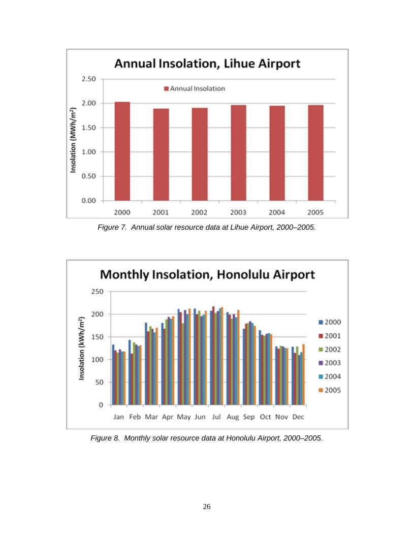
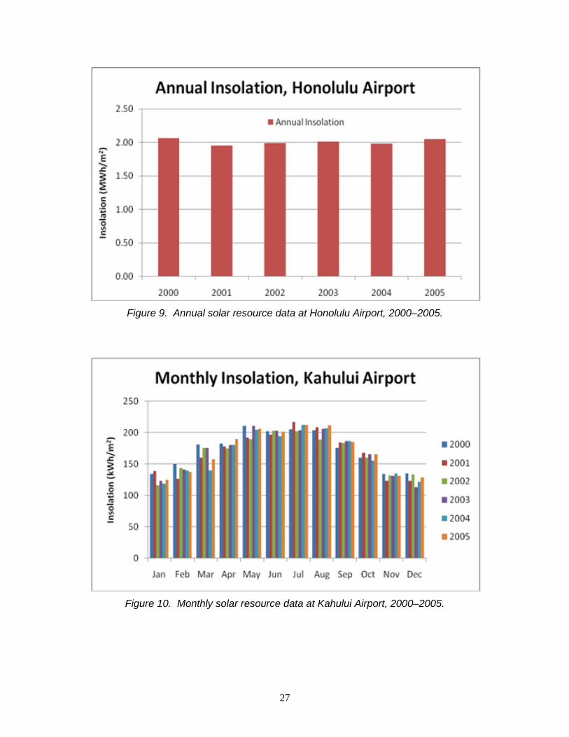
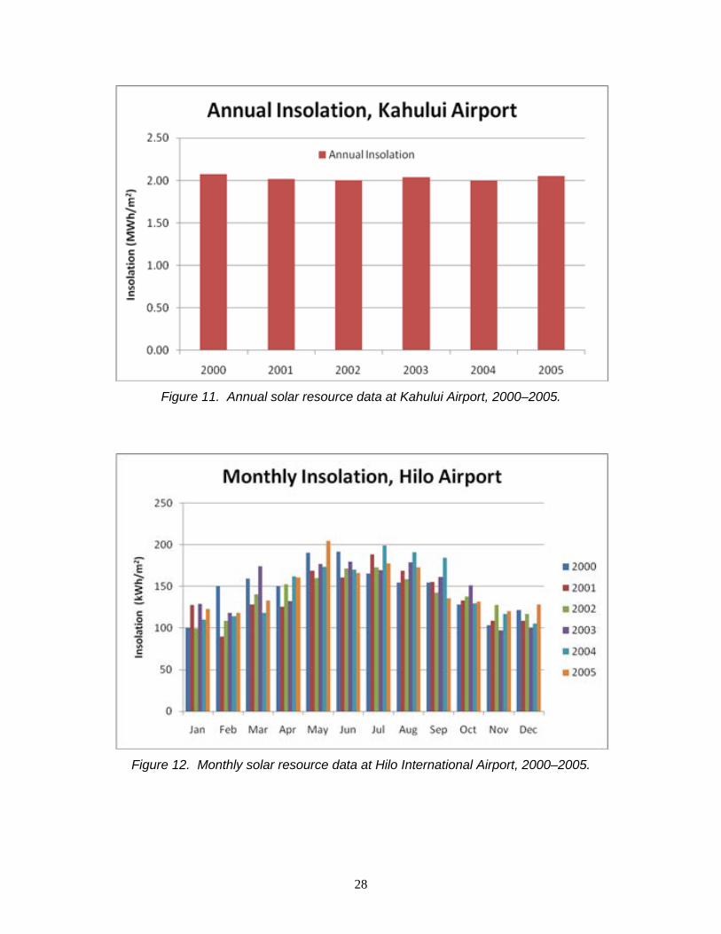
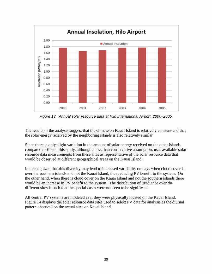
3.2.1 Year-to-Year Comparison Site analysis was performed to compare the measured solar resource data from Lihue Airport, Honolulu Airport, Kahului Airport, and Hilo Airport over a six-year period (2000–2005). Figures 6 through 13 show that slight monthly variation occurs over the years at the different sites, with the solar radiation at its highest from April through September and lowest from October through March, which corresponds to summer and winter seasons respectively. The result of the analysis also shows that the different sites are comparable in the amount of annual radiation received. For all the sites, a total annual solar radiation of about 2.0 MWh/m2 is observed except at Hilo International Airport, where the annual solar radiation is slightly lower, 1.75 MWh/m2. The sites show similarity in the monthly solar radiation and the annual solar radiation when compared to that observed at Lihue International Airport in Kauai.
Figure 6. Monthly solar resource data at Lihue Airport, 2000–2005.
26
Figure 7. Annual solar resource data at Lihue Airport, 2000–2005.
Figure 8. Monthly solar resource data at Honolulu Airport, 2000–2005.
27
Figure 9. Annual solar resource data at Honolulu Airport, 2000–2005.
Figure 10. Monthly solar resource data at Kahului Airport, 2000–2005.
28
Figure 11. Annual solar resource data at Kahului Airport, 2000–2005.
Figure 12. Monthly solar resource data at Hilo International Airport, 2000–2005.
29
Figure 13. Annual solar resource data at Hilo International Airport, 2000–2005.
The results of the analysis suggest that the climate on Kauai Island is relatively constant and that the solar energy received by the neighboring islands is also relatively similar. Since there is only slight variation in the amount of solar energy received on the other islands compared to Kauai, this study, although a less than conservative assumption, uses available solar resource data measurements from these sites as representative of the solar resource data that would be observed at different geographical areas on the Kauai Island. It is recognized that this diversity may lend to increased variability on days when cloud cover is over the southern islands and not the Kauai Island, thus reducing PV benefit to the system. On the other hand, when there is cloud cover on the Kauai Island and not the southern islands there would be an increase in PV benefit to the system. The distribution of irradiance over the different sites is such that the special cases were not seen to be significant. All central PV systems are modeled as if they were physically located on the Kauai Island. Figure 14 displays the solar resource data sites used to select PV data for analysis as the diurnal pattern observed on the actual sites on Kauai Island.
30
Site 1Lihue
Airport 05
Site 3Kahului
Airport 05
Site 2HonoluluAirport 05
Site 4Hilo
Airport 05
Site 5Lihue
Airport 04Site 6
HonoluluAirport 04
Site 7Kahului
Airport 04
SELECTED DATA FOR
SITES
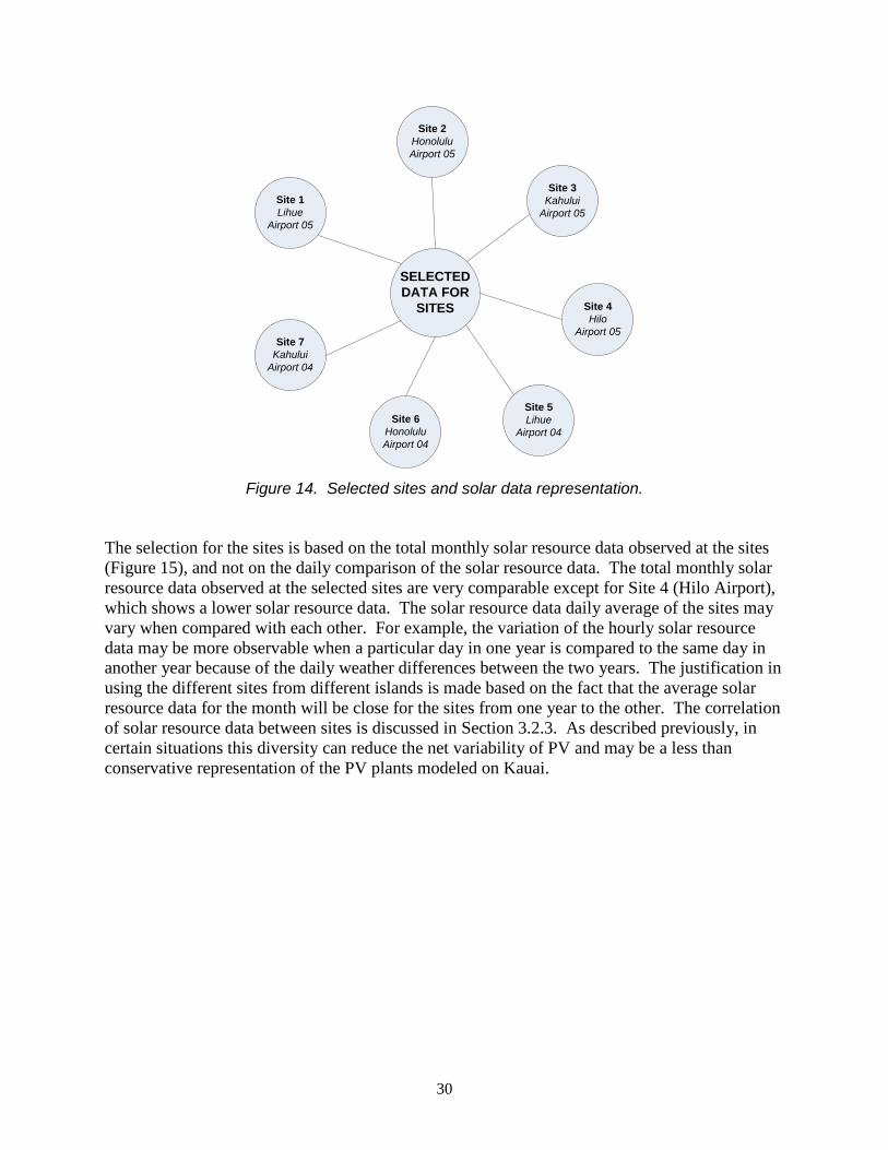
Figure 14. Selected sites and solar data representation.
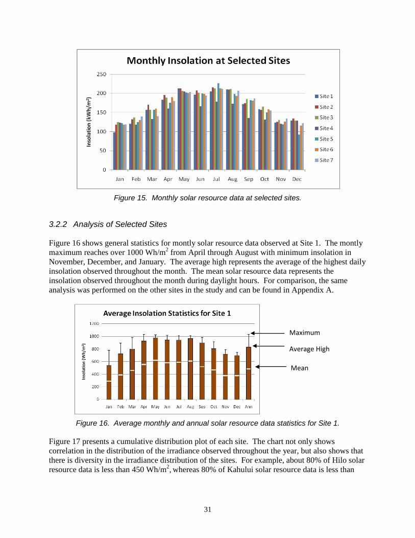
The selection for the sites is based on the total monthly solar resource data observed at the sites (Figure 15), and not on the daily comparison of the solar resource data. The total monthly solar resource data observed at the selected sites are very comparable except for Site 4 (Hilo Airport), which shows a lower solar resource data. The solar resource data daily average of the sites may vary when compared with each other. For example, the variation of the hourly solar resource data may be more observable when a particular day in one year is compared to the same day in another year because of the daily weather differences between the two years. The justification in using the different sites from different islands is made based on the fact that the average solar resource data for the month will be close for the sites from one year to the other. The correlation of solar resource data between sites is discussed in Section 3.2.3. As described previously, in certain situations this diversity can reduce the net variability of PV and may be a less than conservative representation of the PV plants modeled on Kauai.
31
Figure 15. Monthly solar resource data at selected sites.
3.2.2 Analysis of Selected Sites Figure 16 shows general statistics for montly solar resource data observed at Site 1. The montly maximum reaches over 1000 Wh/m2 from April through August with minimum insolation in November, December, and January. The average high represents the average of the highest daily insolation observed throughout the month. The mean solar resource data represents the insolation observed throughout the month during daylight hours. For comparison, the same analysis was performed on the other sites in the study and can be found in Appendix A.
Figure 16. Average monthly and annual solar resource data statistics for Site 1.
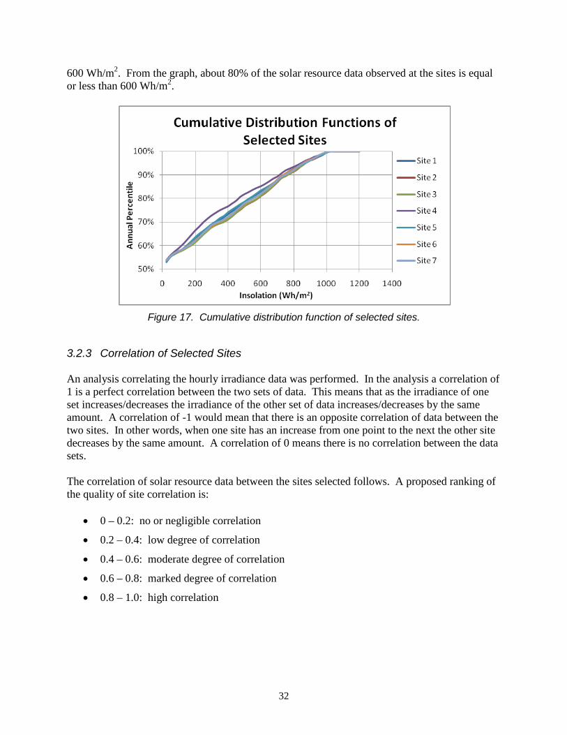
Figure 17 presents a cumulative distribution plot of each site. The chart not only shows correlation in the distribution of the irradiance observed throughout the year, but also shows that there is diversity in the irradiance distribution of the sites. For example, about 80% of Hilo solar resource data is less than 450 Wh/m2, whereas 80% of Kahului solar resource data is less than
Maximum
Average High
Mean
32
600 Wh/m2. From the graph, about 80% of the solar resource data observed at the sites is equal or less than 600 Wh/m2.
Figure 17. Cumulative distribution function of selected sites.
3.2.3 Correlation of Selected Sites An analysis correlating the hourly irradiance data was performed. In the analysis a correlation of 1 is a perfect correlation between the two sets of data. This means that as the irradiance of one set increases/decreases the irradiance of the other set of data increases/decreases by the same amount. A correlation of -1 would mean that there is an opposite correlation of data between the two sites. In other words, when one site has an increase from one point to the next the other site decreases by the same amount. A correlation of 0 means there is no correlation between the data sets. The correlation of solar resource data between the sites selected follows. A proposed ranking of the quality of site correlation is:
• 0 – 0.2: no or negligible correlation
• 0.2 – 0.4: low degree of correlation
• 0.4 – 0.6: moderate degree of correlation
• 0.6 – 0.8: marked degree of correlation
• 0.8 – 1.0: high correlation
33
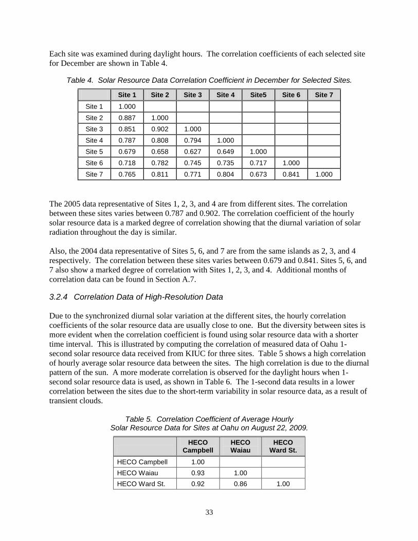
Each site was examined during daylight hours. The correlation coefficients of each selected site for December are shown in Table 4.
Table 4. Solar Resource Data Correlation Coefficient in December for Selected Sites.
Site 1 Site 2 Site 3 Site 4 Site5 Site 6 Site 7 Site 1 1.000
Site 2 0.887 1.000 Site 3 0.851 0.902 1.000
Site 4 0.787 0.808 0.794 1.000 Site 5 0.679 0.658 0.627 0.649 1.000
Site 6 0.718 0.782 0.745 0.735 0.717 1.000 Site 7 0.765 0.811 0.771 0.804 0.673 0.841 1.000
The 2005 data representative of Sites 1, 2, 3, and 4 are from different sites. The correlation between these sites varies between 0.787 and 0.902. The correlation coefficient of the hourly solar resource data is a marked degree of correlation showing that the diurnal variation of solar radiation throughout the day is similar. Also, the 2004 data representative of Sites 5, 6, and 7 are from the same islands as 2, 3, and 4 respectively. The correlation between these sites varies between 0.679 and 0.841. Sites 5, 6, and 7 also show a marked degree of correlation with Sites 1, 2, 3, and 4. Additional months of correlation data can be found in Section A.7.
3.2.4 Correlation Data of High-Resolution Data Due to the synchronized diurnal solar variation at the different sites, the hourly correlation coefficients of the solar resource data are usually close to one. But the diversity between sites is more evident when the correlation coefficient is found using solar resource data with a shorter time interval. This is illustrated by computing the correlation of measured data of Oahu 1-second solar resource data received from KIUC for three sites. Table 5 shows a high correlation of hourly average solar resource data between the sites. The high correlation is due to the diurnal pattern of the sun. A more moderate correlation is observed for the daylight hours when 1-second solar resource data is used, as shown in Table 6. The 1-second data results in a lower correlation between the sites due to the short-term variability in solar resource data, as a result of transient clouds.
Table 5. Correlation Coefficient of Average Hourly Solar Resource Data for Sites at Oahu on August 22, 2009.
HECO
Campbell HECO Waiau
HECO Ward St.
HECO Campbell 1.00 HECO Waiau 0.93 1.00 HECO Ward St. 0.92 0.86 1.00
34
Table 6. Correlation Coefficient of 1–Second Solar Resource Data for Oahu Data on August 22, 2009.
HECO Campbell
HECO Waiau
HECO Ward St.
HECO Campbell 1.00 HECO Waiau 0.54 1.00
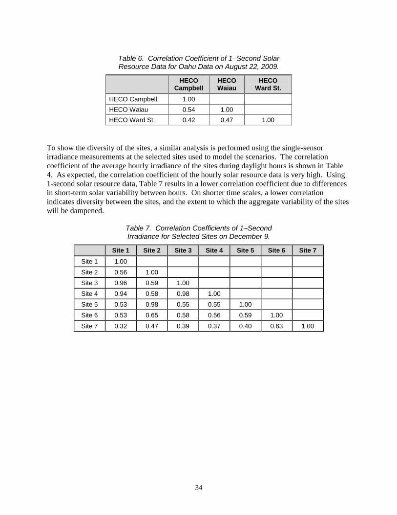
HECO Ward St. 0.42 0.47 1.00 To show the diversity of the sites, a similar analysis is performed using the single-sensor irradiance measurements at the selected sites used to model the scenarios. The correlation coefficient of the average hourly irradiance of the sites during daylight hours is shown in Table 4. As expected, the correlation coefficient of the hourly solar resource data is very high. Using 1-second solar resource data, Table 7 results in a lower correlation coefficient due to differences in short-term solar variability between hours. On shorter time scales, a lower correlation indicates diversity between the sites, and the extent to which the aggregate variability of the sites will be dampened.
Table 7. Correlation Coefficients of 1–Second Irradiance for Selected Sites on December 9.
Site 1 Site 2 Site 3 Site 4 Site 5 Site 6 Site 7 Site 1 1.00 Site 2 0.56 1.00
Site 3 0.96 0.59 1.00 Site 4 0.94 0.58 0.98 1.00
Site 5 0.53 0.98 0.55 0.55 1.00 Site 6 0.53 0.65 0.58 0.56 0.59 1.00
Site 7 0.32 0.47 0.39 0.37 0.40 0.63 1.00
35
3.3 Scenario Analysis
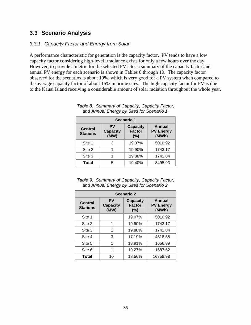
3.3.1 Capacity Factor and Energy from Solar A performance characteristic for generation is the capacity factor. PV tends to have a low capacity factor considering high-level irradiance exists for only a few hours over the day. However, to provide a metric for the selected PV sites a summary of the capacity factor and annual PV energy for each scenario is shown in Tables 8 through 10. The capacity factor observed for the scenarios is about 19%, which is very good for a PV system when compared to the average capacity factor of about 15% in prime sites. The high capacity factor for PV is due to the Kauai Island receiving a considerable amount of solar radiation throughout the whole year.
Table 8. Summary of Capacity, Capacity Factor, and Annual Energy by Sites for Scenario 1.
Scenario 1
Central Stations
PV Capacity
(MW)
Capacity Factor
(%)
Annual PV Energy
(MWh) Site 1 3 19.07% 5010.92 Site 2 1 19.90% 1743.17 Site 3 1 19.88% 1741.84 Total 5 19.40% 8495.93
Table 9. Summary of Capacity, Capacity Factor, and Annual Energy by Sites for Scenario 2.
Scenario 2
Central Stations
PV Capacity
(MW)
Capacity Factor
(%)
Annual PV Energy
(MWh) Site 1 19.07% 5010.92 Site 2 1 19.90% 1743.17 Site 3 1 19.88% 1741.84 Site 4 3 17.19% 4518.55 Site 5 1 18.91% 1656.89 Site 6 1 19.27% 1687.62 Total 10 18.56% 16358.98
36
Table 10. Summary of Capacity, Capacity Factor,
and Annual Energy by Sites for Scenario 3.
Scenario 3
Central Stations
PV Capacity
(MW)
Capacity Factor
(%)
Annual PV Energy
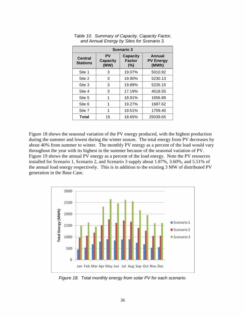
(MWh) Site 1 3 19.07% 5010.92 Site 2 3 19.90% 5230.13 Site 3 3 19.89% 5226.15 Site 4 3 17.19% 4518.55 Site 5 1 18.91% 1656.89 Site 6 1 19.27% 1687.62 Site 7 1 19.51% 1709.40 Total 15 18.65% 25039.65
Figure 18 shows the seasonal variation of the PV energy produced, with the highest production during the summer and lowest during the winter season. The total energy from PV decreases by about 40% from summer to winter. The monthly PV energy as a percent of the load would vary throughout the year with its highest in the summer because of the seasonal variation of PV. Figure 19 shows the annual PV energy as a percent of the load energy. Note the PV resources installed for Scenario 1, Scenario 2, and Scenario 3 supply about 1.87%, 3.60%, and 5.51% of the annual load energy respectively. This is in addition to the existing 3 MW of distributed PV generation in the Base Case.
Figure 18. Total monthly energy from solar PV for each scenario.

37
Figure 19. Annual energy as a percent of load energy.
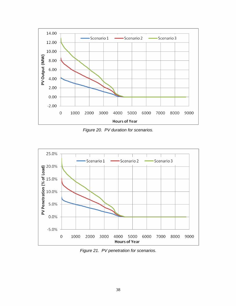
3.3.2 PV Duration Figures 20 and 21 show the PV duration curve and the PV penetration as a percent of the load throughout the year. The x-axis represents 8760 hours of the year. The PV duration curve is obtained by sorting the PV output for each scenario. The charts show as expected the availability of PV for 50% of the year when the sun is shining. With increasing PV penetration level, regulation becomes more important because of the increased net load variability. Figure 21 shows the PV penetration of each scenario throughout the year. The PV penetration as percentage of load is calculated by expressing the chronological PV output as a percent of the corresponding hourly load for the year 2011. Even though PV resources are installed to supply about 1.87%, 3.60%, and 5.51% of the annual load energy for Scenario 1, Scenario 2, and Scenario 3 respectively, higher PV penetration can be observed for PV at different times during the year. For example, excluding the existing 3 MW of distributed PV generation that currently exists on the system, throughout the year peak PV output can reach 8%, 15%, and 23% of the instantaneous system load for Scenario 1, Scenario 2, and Scenario 3 respectively.
38
Figure 20. PV duration for scenarios.
Figure 21. PV penetration for scenarios.
39
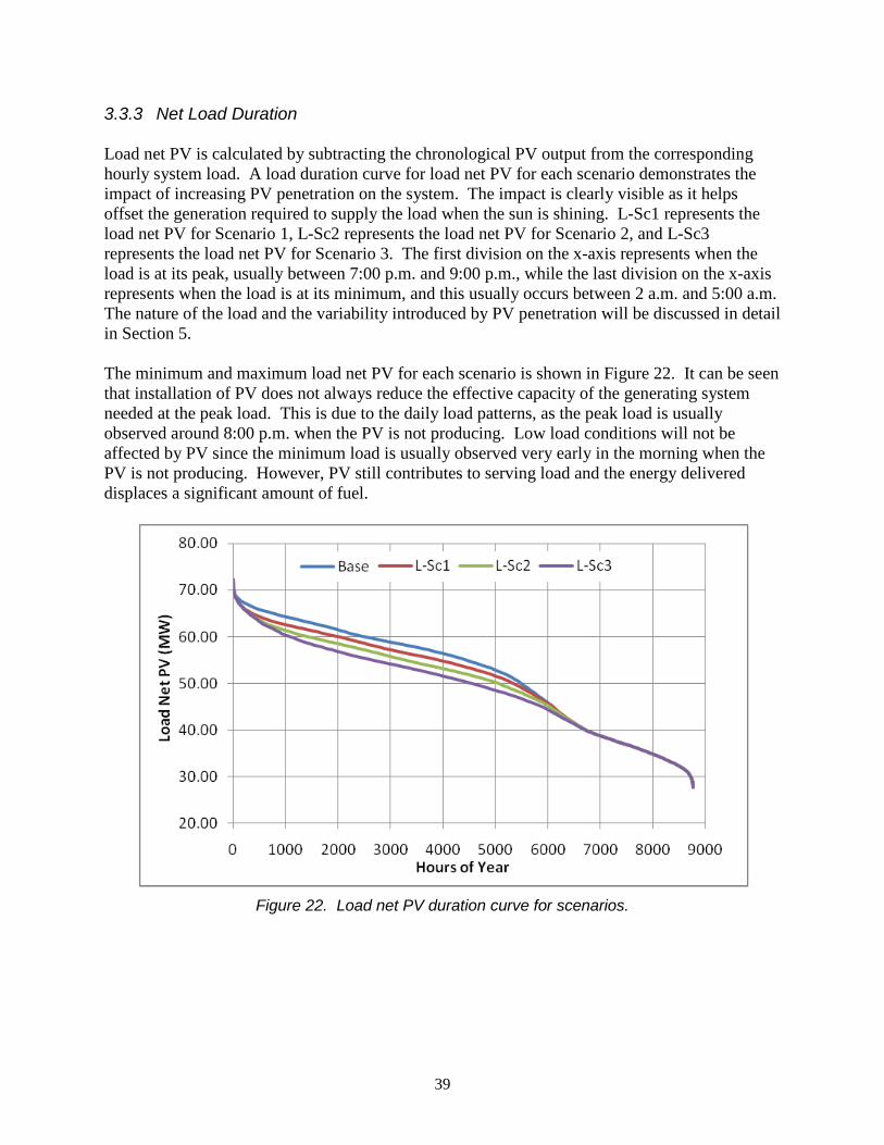
3.3.3 Net Load Duration Load net PV is calculated by subtracting the chronological PV output from the corresponding hourly system load. A load duration curve for load net PV for each scenario demonstrates the impact of increasing PV penetration on the system. The impact is clearly visible as it helps offset the generation required to supply the load when the sun is shining. L-Sc1 represents the load net PV for Scenario 1, L-Sc2 represents the load net PV for Scenario 2, and L-Sc3 represents the load net PV for Scenario 3. The first division on the x-axis represents when the load is at its peak, usually between 7:00 p.m. and 9:00 p.m., while the last division on the x-axis represents when the load is at its minimum, and this usually occurs between 2 a.m. and 5:00 a.m. The nature of the load and the variability introduced by PV penetration will be discussed in detail in Section 5. The minimum and maximum load net PV for each scenario is shown in Figure 22. It can be seen that installation of PV does not always reduce the effective capacity of the generating system needed at the peak load. This is due to the daily load patterns, as the peak load is usually observed around 8:00 p.m. when the PV is not producing. Low load conditions will not be affected by PV since the minimum load is usually observed very early in the morning when the PV is not producing. However, PV still contributes to serving load and the energy delivered displaces a significant amount of fuel.
Figure 22. Load net PV duration curve for scenarios.
40
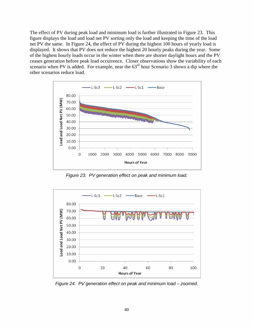
The effect of PV during peak load and minimum load is further illustrated in Figure 23. This figure displays the load and load net PV sorting only the load and keeping the time of the load net PV the same. In Figure 24, the effect of PV during the highest 100 hours of yearly load is displayed. It shows that PV does not reduce the highest 20 hourly peaks during the year. Some of the highest hourly loads occur in the winter when there are shorter daylight hours and the PV ceases generation before peak load occurrence. Closer observations show the variability of each scenario when PV is added. For example, near the 63rd hour Scenario 3 shows a dip where the other scenarios reduce load.
Figure 23. PV generation effect on peak and minimum load.
Figure 24. PV generation effect on peak and minimum load – zoomed.

41
4 Methodology
Electric power system operations control a diverse set of power generation that for the most part has been coordinating thermal and hydro resources with smaller (proportionally) amounts of renewable resources such as wind, solar PV, geothermal and bio gas, to list a few. PV generation has the potential to increase net load variability in the short time frame. For this reason an investigation was performed to examine the impact of PV variability on the existing KIUC system for each of the PV scenarios. This investigation focused on regulation to control system frequency. In order to schedule generation and reserve resources in a control area that accommodates PV power, the time-varying patterns of the PV power production have to be taken into account. Overall, the additional system fluctuations that result from adding sizable PV plants are a function of the level of the PV penetration to the total system. PV generation output fluctuations principally drive the additional requirements and costs of balancing the host power system in the operational time scale (seconds to hours). Based on the varying production patterns of PV generation, a system operator may find that changes in scheduling and unit commitment of non-PV plants may result in a loss or a benefit to the system. In general, PV power introduces varying production patterns and uncertainties that are different than what has been customary operation with hydro and thermal type generation. This difference can require an increase in use of additional resources to maintain balance. These resources include operational reserves to recover instantaneous changes in the balance between load and generation on the time scale of seconds (regulation reserves) and economic dispatch to adjust the output of units to follow longer trends in the net load (load-following reserves). 4.1 KIUC System Model The purpose of modeling the KUIC AGC system is to analyze the sub-hour PV generation impacts in order to estimate the additional flexibility (regulation reserves) that would be required to manage the control area with significant PV generation. The analysis and simulation are based on 15-second system frequency data for the month of December (2011) and the 15-minute load data for the same period. The goal is to develop a model that uses load and load net PV variations as input while providing output of the required additional regulating capacity in order to maintain the balance of the system (i.e., keep the frequency close to the provided 15-second profile). KIUC provided samples of 15-second-frequency performance data that was used as a baseline for tuning the system model. The procedure for determining the required generation variations is as follows:
1. Using the 15-minute load data, tune the control parameters (AGC gain, inertia) of the model. The simulation frequency output has to follow the actual system frequency on a 15-second base resulting in a 15-second load deviation profile.

42
2. Compute the load net PV data, based on the obtained 15-second load deviation data and 15-second solar resource data. Section A.2 provides information about the 15-second data.
3. Use the resulting 15-second load net PV data, from each PV penetration scenario, as simulation inputs.
4. The findings from the load-only and load net PV simulations (i.e., required generation variations) become inputs to later analytical processes; see Section 5.2 and Section 5.3.
4.1.1 System Model The KIUC system is an electrical island operation with no ties to adjacent islands. Thus KIUC has sole responsibility to manage generation and afford their customers adequate reliability and system stability with minimum service interruptions. Because the system operates as an electrical island, the Kauai power system is modeled as an isolated power system consisting of a single generating unit that supplies a net load with specified frequency characteristics (see Figure 25). Note that the model excludes transmission and distribution lines, assuming they have no impact on the system behavior. Based on the magnitudes of the changes in the load, the droop characteristics of the governor, and a supplementary control responsible for keeping the system frequency close to the nominal frequency (i.e., 60 Hz), the simulation calculates the corresponding frequency changes. The model was configured and simulated using the visual block diagram language VisSim. Figure 25 shows the block diagram of the model. It consists of the following components and their tasks.2
• Supplementary Control Model: This component models adjustments of the load reference set point, in order to force the frequency deviations to zero.
• Load Reference Set Point: Reference unit output to force the frequency deviations to zero.
• Governor Model: This component models adjustment of the valve to change the mechanical power output to compensate for load changes.
• Per Unit Change in Valve Position: Position of the valve that controls emission of the steam into the turbine.
• Governor Net Gain Model: This component determines the change in the unit’s output for a given change in frequency.
• Prime–Mover Model: This component models a turbine by relating the position of the valve that controls emission of steam into the turbine to the power output of the turbine.
• Per Unit Load Change: Net load drawn by the system (input).
2 Allen J. Wood and Bruce F. Wollenberg, Power Generation Operation and Control, John Wiley & Sons, 1984.

43
Figure 25. Block diagram of used system model with supplementary control.
• Rotating Mass and Load: A component that combines the following:
o Generator Model: This component models positive and negative acceleration of the machine due to differences in mechanical and electrical torque, deviation of speed (Δω), and deviation of phase angle (Δδ). Generation is ramped up and down while inertia is assumed to be the same across all scenarios.
o Load Model: This component models the effect of a change in frequency on the net load drawn by the system at a given per unit base (i.e., 75 MW in this study).
• Per Unit Speed Change: Deviation of the frequency from the nominal 60 Hz (output).
• Per Unit Change in Unit Output: Changes in generation due to changes in frequency.
4.1.2 System Simulation of Base Case As described in Section 4.1.1, the simulation implemented to represent the model of the control area uses load variability as input. The model accepts load as input and computes the system output frequency by matching a generation profile to the load. In a perfect world the generation would exactly match the load, resulting in a system frequency of 60 Hz. In reality the frequency varies about the 60 Hz target. KIUC provided corresponding load and frequency data for several days of real-time operations. The model required tuning to calculate an output frequency for the input load that closely matched the given frequency. To do this a profile of generator variability was used in the model. The profile was systematically adjusted until the resulting frequency output for the given load input closely represented the measured frequency of the system. The following figures display the data representation of this process. The KIUC system load profile is shown in Figure 26. The system generation serves to produce the KIUC system
Load Refer-
ence Set Point
Per Unit Speed
Change
Per Unit Change in
Unit Output
Supplementary
Control
Governor
Prime Mover
Rotating
Mass & Load
Governor Net Gain
+ -
+
-
Per Unit Load
Change
Per Unit Change in
Valve Position

44
frequency (Figure 27). The change in system load (Figure 28) must be followed by a comparable change in generation to maintain system frequency. The lead or lag of generation load following causes frequency variations as shown in the measured frequency (Figure 27). The model without a generation profile would operate perfectly at 60 Hz, so the generation profile was created and tuned (Figure 29) to cause the models output frequency to have behavior similar to the measured system frequency. Using the generator profile the modeled output frequency is shown super imposed on the system frequency in Figure 30. A sample hour is shown in Figure 31.
Figure 26. Load profile for a one-day period.
Figure 27. System frequency profile for a one-day period.
45
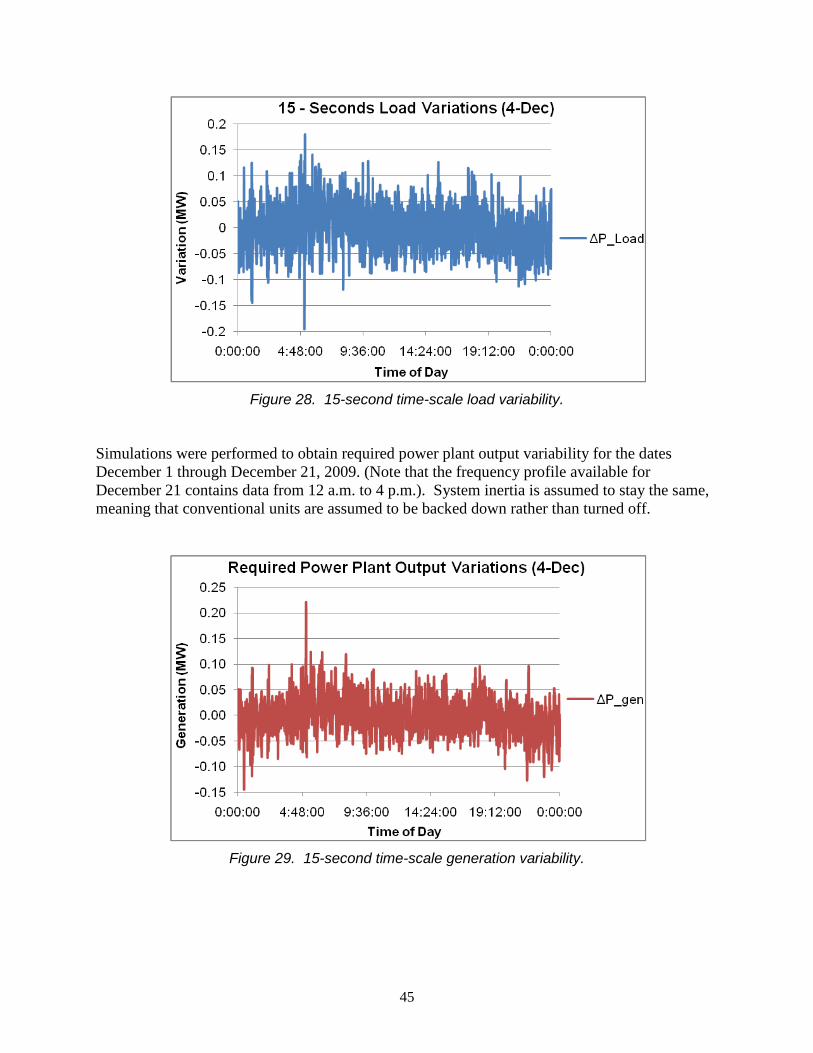
Figure 28. 15-second time-scale load variability.
Simulations were performed to obtain required power plant output variability for the dates December 1 through December 21, 2009. (Note that the frequency profile available for December 21 contains data from 12 a.m. to 4 p.m.). System inertia is assumed to stay the same, meaning that conventional units are assumed to be backed down rather than turned off.
Figure 29. 15-second time-scale generation variability.
46
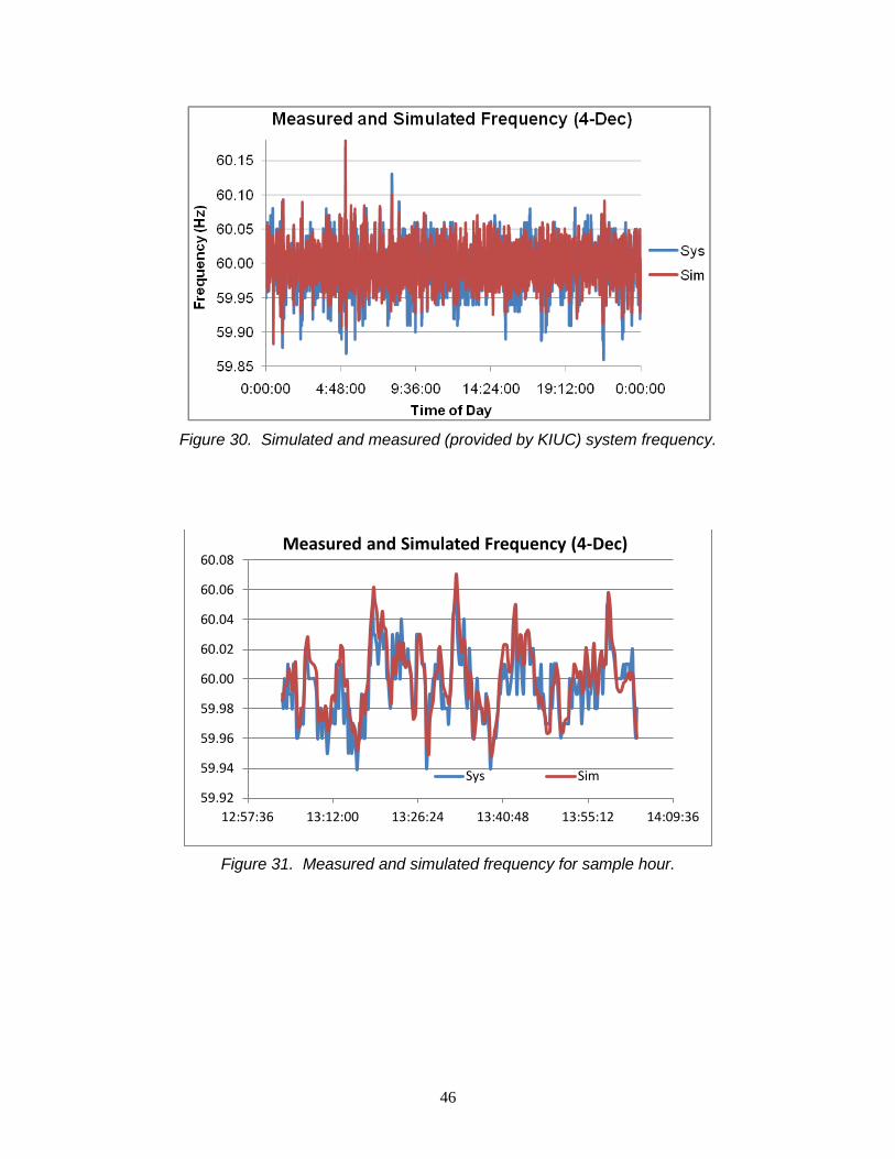
Figure 30. Simulated and measured (provided by KIUC) system frequency.
Figure 31. Measured and simulated frequency for sample hour.
59.92
59.94
59.96
59.98
60.00
60.02
60.04
60.06
60.08
12:57:36 13:12:00 13:26:24 13:40:48 13:55:12 14:09:36
Measured and Simulated Frequency (4-Dec)
Sys Sim
47
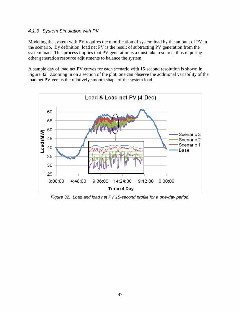
4.1.3 System Simulation with PV Modeling the system with PV requires the modification of system load by the amount of PV in the scenario. By definition, load net PV is the result of subtracting PV generation from the system load. This process implies that PV generation is a must take resource, thus requiring other generation resource adjustments to balance the system. A sample day of load net PV curves for each scenario with 15-second resolution is shown in Figure 32. Zooming in on a section of the plot, one can observe the additional variability of the load net PV versus the relatively smooth shape of the system load.
Figure 32. Load and load net PV 15-second profile for a one-day period.
48
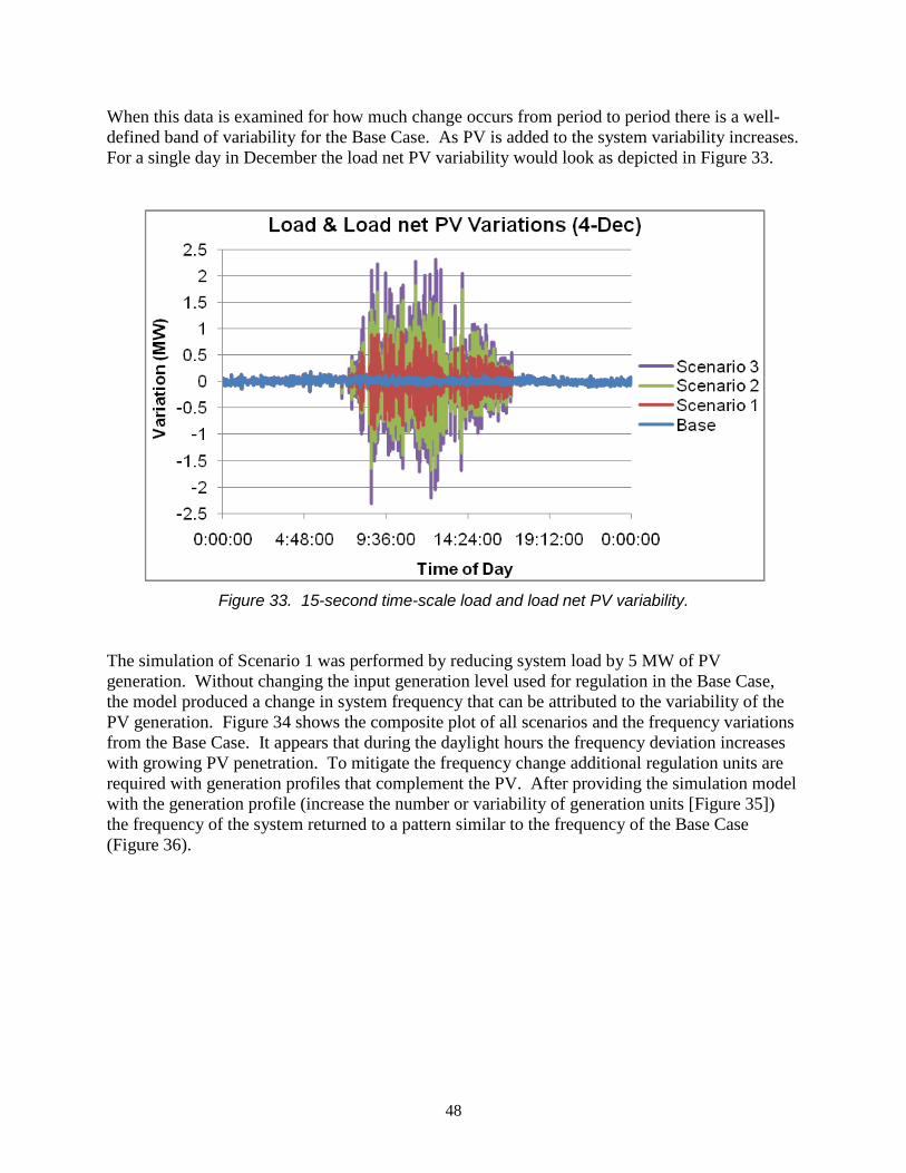
When this data is examined for how much change occurs from period to period there is a well-defined band of variability for the Base Case. As PV is added to the system variability increases. For a single day in December the load net PV variability would look as depicted in Figure 33.
Figure 33. 15-second time-scale load and load net PV variability.
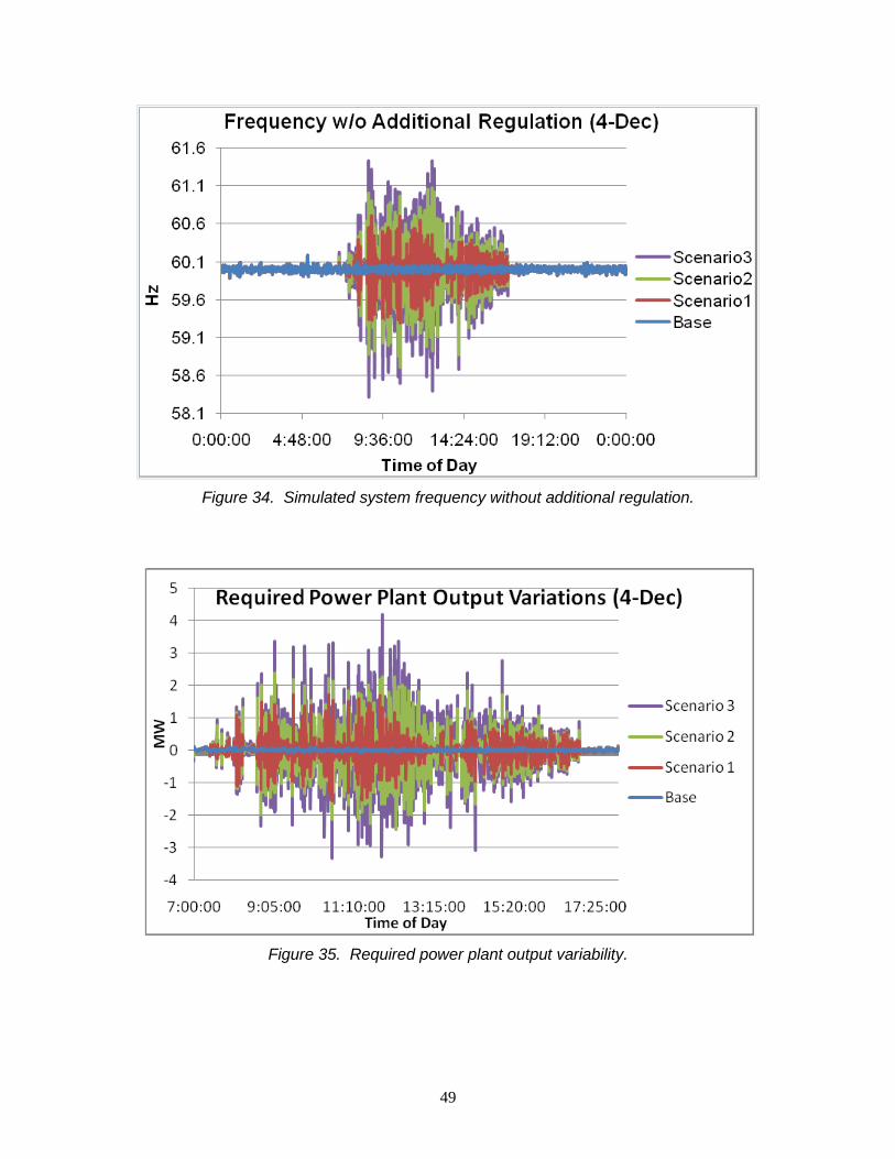
The simulation of Scenario 1 was performed by reducing system load by 5 MW of PV generation. Without changing the input generation level used for regulation in the Base Case, the model produced a change in system frequency that can be attributed to the variability of the PV generation. Figure 34 shows the composite plot of all scenarios and the frequency variations from the Base Case. It appears that during the daylight hours the frequency deviation increases with growing PV penetration. To mitigate the frequency change additional regulation units are required with generation profiles that complement the PV. After providing the simulation model with the generation profile (increase the number or variability of generation units [Figure 35]) the frequency of the system returned to a pattern similar to the frequency of the Base Case (Figure 36).
49
Figure 34. Simulated system frequency without additional regulation.
Figure 35. Required power plant output variability.
50
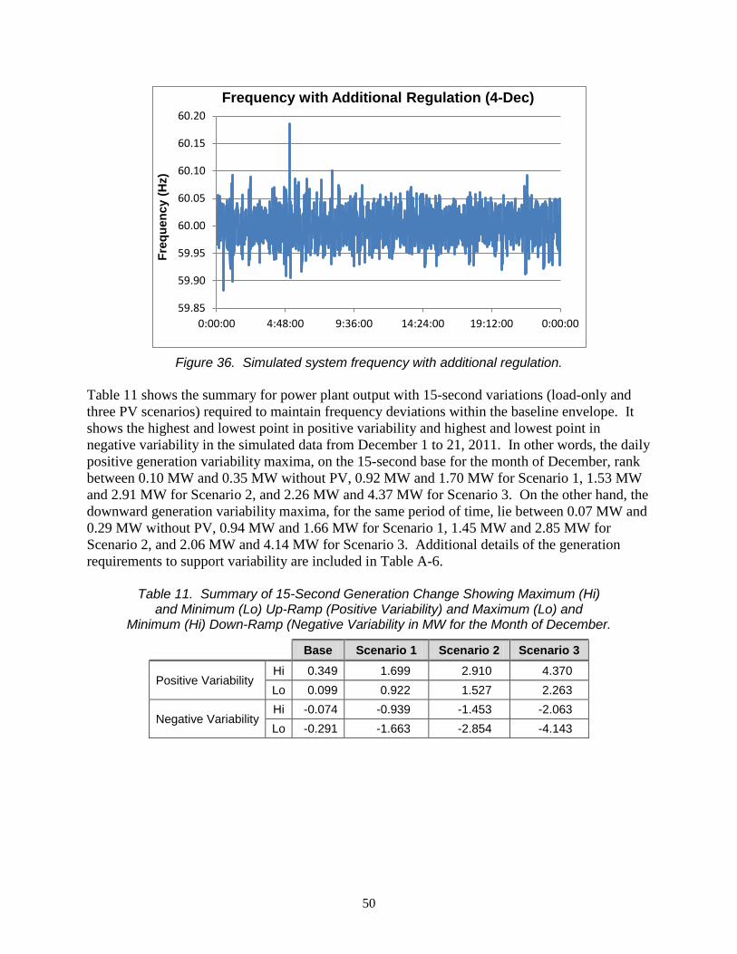
Figure 36. Simulated system frequency with additional regulation.
Table 11 shows the summary for power plant output with 15-second variations (load-only and three PV scenarios) required to maintain frequency deviations within the baseline envelope. It shows the highest and lowest point in positive variability and highest and lowest point in negative variability in the simulated data from December 1 to 21, 2011. In other words, the daily positive generation variability maxima, on the 15-second base for the month of December, rank between 0.10 MW and 0.35 MW without PV, 0.92 MW and 1.70 MW for Scenario 1, 1.53 MW and 2.91 MW for Scenario 2, and 2.26 MW and 4.37 MW for Scenario 3. On the other hand, the downward generation variability maxima, for the same period of time, lie between 0.07 MW and 0.29 MW without PV, 0.94 MW and 1.66 MW for Scenario 1, 1.45 MW and 2.85 MW for Scenario 2, and 2.06 MW and 4.14 MW for Scenario 3. Additional details of the generation requirements to support variability are included in Table A-6.
Table 11. Summary of 15-Second Generation Change Showing Maximum (Hi) and Minimum (Lo) Up-Ramp (Positive Variability) and Maximum (Lo) and
Minimum (Hi) Down-Ramp (Negative Variability in MW for the Month of December.
Base Scenario 1 Scenario 2 Scenario 3
Positive Variability Hi 0.349 1.699 2.910 4.370 Lo 0.099 0.922 1.527 2.263
Negative Variability Hi -0.074 -0.939 -1.453 -2.063 Lo -0.291 -1.663 -2.854 -4.143
59.85
59.90
59.95
60.00
60.05
60.10
60.15
60.20
0:00:00 4:48:00 9:36:00 14:24:00 19:12:00 0:00:00
Freq
uenc
y (H
z)
Frequency with Additional Regulation (4-Dec)

51
4.2 Marginal Unit Identification When system generation is replaced by an alternative resource, be it load control or a renewable resource, the remaining generation committed to serve system load can commit and/or will dispatch differently. In general, the overall cost of operating the generation fleet decreases by the cost of the offset generation. The marginal unit in this study is considered to be the unit that would be used to either serve the next MW of load or the resource backed down to avoid over-generation. Identifying the marginal units for the study year 2011 was based on results taken from UPLAN for the monthly marginal cost and the hourly load profile. The UPLAN data provided the marginal cost in $/MWh and unit occurrence in hours. For this analysis UPLAN operation output data for the year 2010 were used. The procedure for identifying the marginal units for the depicted scenarios is as follows:
1. Arrange monthly load data in descending order.
2. Apply marginal units in reversed merit order (high priced units first) based on the occurrence starting with the first hour.
3. Identify the minimum and maximum loads within which the particular unit is to be operated.
4. Calculate monthly load net PV profiles and arrange them in descending order.
5. Identify the load regions for the units based on load-only load boundaries.
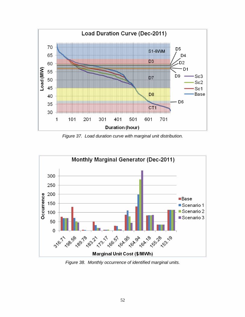
6. Estimate the marginal unit occurrence for every unit depending on the depicted scenario. Figure 37 shows the load and load net PV duration curves together with the marginal units operated at the depicted month (December). The occurrence of a marginal unit for a given load profile equals the length of the corresponding duration curve within the unit’s marked area. The marginal unit cost estimation is based on the identified monthly occurrence of every unit for a depicted scenario. Figure 38 shows the occurrence of the marginal units for a single month with respect to the scenarios (Marginal Unit Cost represent the corresponding marginal units – i.e., 316.71 $/MWh corresponds to unit S1-8MW-Block Loaded, 198.56 $/MWh to unit D3, 189.78 $/MWh to unit D5, etc.). With increasing PV penetration level the occurrence shifts to less-expensive units, reducing the overall marginal cost. This is described in more detail in Section 5.3.1. Monthly marginal generation costs are summarized in Table A-7. Figure A-9 shows the monthly duration curves for the different scenarios in the study.
52
Figure 37. Load duration curve with marginal unit distribution.
Figure 38. Monthly occurrence of identified marginal units.

53
4.3 Regulation Change Estimation The regulation change estimation is based on the difference between the sub-hourly variability of the net load at the different penetration level of PV and the sub-hourly variability of the net load for the Base Case. In other words, we assume that the variability between maximum and minimum load within a given time period (1 hour) is supported by generation designated for regulation. This generation is typically comprised of one or more generating units running on the margin that is identified specifically for regulation support. When PV is added to the system the effect of PV variability on the system is measured by examining load net PV within the same time period and comparing the difference to the load only. Again the load net PV variability is supported by one or more generators on the margin. The introduction of PV to the system can impact load in three ways:
1. It can reduce the difference in net load change from one period to the next.
2. It can increase the amount of net load change from one period to the next.
3. It can have no change on net load from one period to the next. The results of this study show that PV impacts load by increasing the amount of net load variability. Regulation required to support increased variability is necessary to maintain system frequency. The amount of additional regulation energy depends upon the penetration level of PV and the variability of the solar resource data. It was determined that as PV is added to the system the amount of regulation energy required to maintain system frequency will increase. To capture the amount of generation required to support the inter-hour variability sub-hourly data was examined. The change in load and net load was examined with 15-second resolution data and it was noted that the change in load and change in load net PV showed greater variability than what was seen at the hourly resolution. Based on these findings the study identified the greatest change within the hour and identified this to be the amount of required regulation to support the additional PV. The amount of energy required within the hour can be supported by one or more generating units that typically would be operating on the margin. An example of sub-hourly load change is depicted in Figure 39. It can be seen that the range for the Base Case requires a set of generators to support 1.3 MW in load variability over the hour (Figure 40). The PV added in scenario 3 shows an increase in load net PV variability of 5 MW (Figure 39). This is an increase of 3.7 MW of variability over the Base Case. In other words, in order to maintain system frequency when 15 MW of PV are added to the system an additional 3.7 MW of on-line regulation generation would be required. Due to increased variability of load net PV the number of required regulating units will have an impact to the KIUC regulation cost.
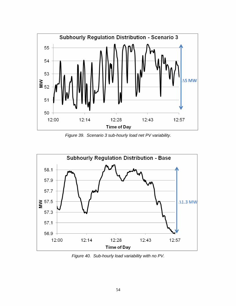
54
Figure 39. Scenario 3 sub-hourly load net PV variability.
Figure 40. Sub-hourly load variability with no PV.
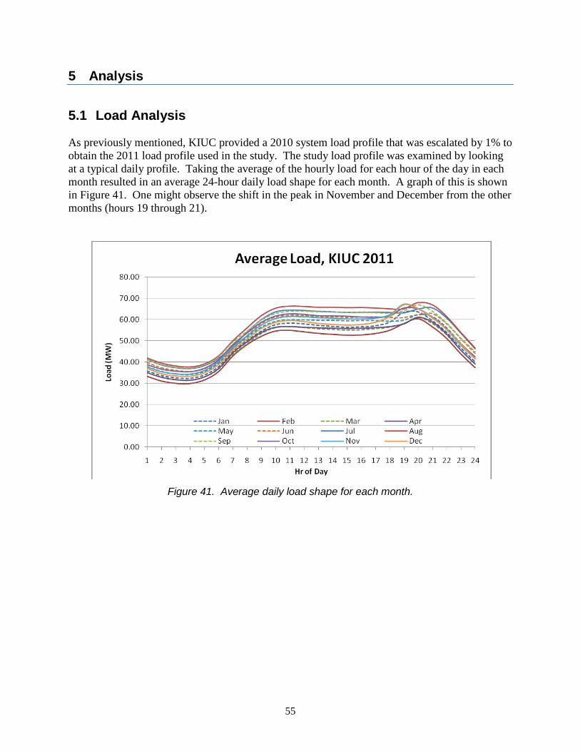
55
5 Analysis
5.1 Load Analysis As previously mentioned, KIUC provided a 2010 system load profile that was escalated by 1% to obtain the 2011 load profile used in the study. The study load profile was examined by looking at a typical daily profile. Taking the average of the hourly load for each hour of the day in each month resulted in an average 24-hour daily load shape for each month. A graph of this is shown in Figure 41. One might observe the shift in the peak in November and December from the other months (hours 19 through 21).
Figure 41. Average daily load shape for each month.
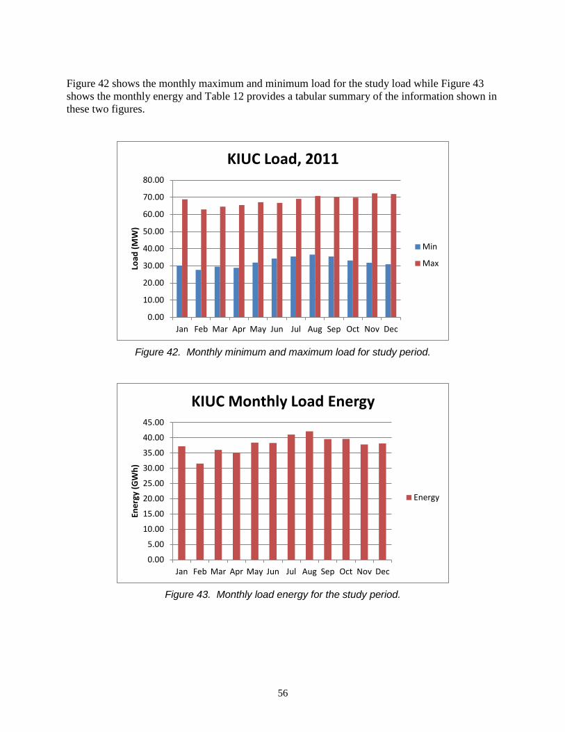
56
Figure 42 shows the monthly maximum and minimum load for the study load while Figure 43 shows the monthly energy and Table 12 provides a tabular summary of the information shown in these two figures.
Figure 42. Monthly minimum and maximum load for study period.
Figure 43. Monthly load energy for the study period.
0.00
10.00
20.00
30.00
40.00
50.00
60.00
70.00
80.00
Jan Feb Mar Apr May Jun Jul Aug Sep Oct Nov Dec
Load
(MW
)
KIUC Load, 2011
Min
Max
0.00
5.00
10.00
15.00
20.00
25.00
30.00
35.00
40.00
45.00
Jan Feb Mar Apr May Jun Jul Aug Sep Oct Nov Dec
Ener
gy (G
Wh)
KIUC Monthly Load Energy
Energy
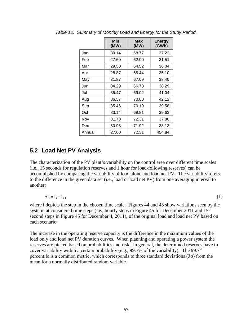
57
Table 12. Summary of Monthly Load and Energy for the Study Period.
Min (MW)
Max (MW)
Energy (GWh)
Jan 30.14 68.77 37.22 Feb 27.60 62.90 31.51 Mar 29.50 64.52 36.04 Apr 28.87 65.44 35.10 May 31.87 67.09 38.40 Jun 34.29 66.73 38.29 Jul 35.47 69.02 41.04 Aug 36.57 70.80 42.12 Sep 35.46 70.19 39.58 Oct 33.14 69.81 39.63 Nov 31.78 72.31 37.80 Dec 30.93 71.92 38.13 Annual 27.60 72.31 454.84
5.2 Load Net PV Analysis The characterization of the PV plant’s variability on the control area over different time scales (i.e., 15 seconds for regulation reserves and 1 hour for load-following reserves) can be accomplished by comparing the variability of load alone and load net PV. The variability refers to the difference in the given data set (i.e., load or load net PV) from one averaging interval to another: ΔLi = Li – Li-1 (1)
where i depicts the step in the chosen time scale. Figures 44 and 45 show variations seen by the system, at considered time steps (i.e., hourly steps in Figure 45 for December 2011 and 15-second steps in Figure 45 for December 4, 2011), of the original load and load net PV based on each scenario. The increase in the operating reserve capacity is the difference in the maximum values of the load only and load net PV duration curves. When planning and operating a power system the reserves are picked based on probabilities and risk. In general, the determined reserves have to cover variability within a certain probability (e.g., 99.7% of the variability). The 99.7th percentile is a common metric, which corresponds to three standard deviations (3σ) from the mean for a normally distributed random variable.
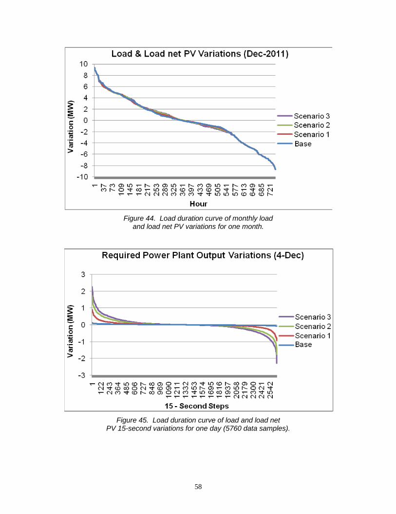
58
Figure 44. Load duration curve of monthly load
and load net PV variations for one month.
Figure 45. Load duration curve of load and load net
PV 15-second variations for one day (5760 data samples).
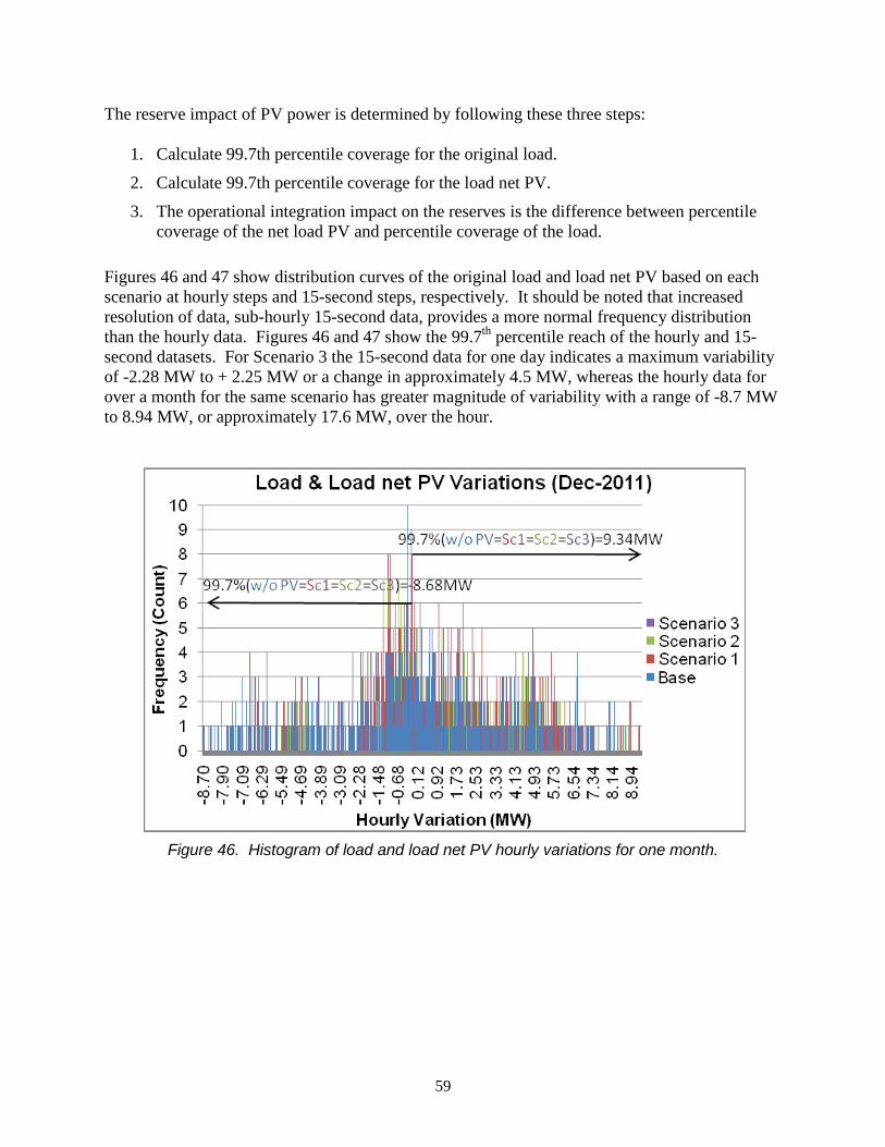
59
The reserve impact of PV power is determined by following these three steps:
1. Calculate 99.7th percentile coverage for the original load.
2. Calculate 99.7th percentile coverage for the load net PV.
3. The operational integration impact on the reserves is the difference between percentile coverage of the net load PV and percentile coverage of the load.
Figures 46 and 47 show distribution curves of the original load and load net PV based on each scenario at hourly steps and 15-second steps, respectively. It should be noted that increased resolution of data, sub-hourly 15-second data, provides a more normal frequency distribution than the hourly data. Figures 46 and 47 show the 99.7th percentile reach of the hourly and 15-second datasets. For Scenario 3 the 15-second data for one day indicates a maximum variability of -2.28 MW to + 2.25 MW or a change in approximately 4.5 MW, whereas the hourly data for over a month for the same scenario has greater magnitude of variability with a range of -8.7 MW to 8.94 MW, or approximately 17.6 MW, over the hour.
Figure 46. Histogram of load and load net PV hourly variations for one month.

60
Figure 47. Histogram of load and load net PV 15-second variations for one day.
Table A-8 shows the details of the monthly 99.7th percentile coverage for the hourly load and load net PV positive variability and increase in variability for the study period. It is interesting to note while there is neither an increase nor a decrease in variability for the months November through March, there is a decrease in variability for the remaining months April through October. That means that when PV power is introduced to the control area no additional load-following reserves are required for the months November through March. However, during months April through October, due to increasing daylight hours, PV power output increasingly affects the peak variations in the load, which occur in early evening hours (7 p.m.–9 p.m.). Therefore, fewer load-following reserves are required for the months April through October, with the highest decrease during the month of May. Table 13 shows the summary for the 99.7th percentile coverage for the month of May. In general, during this month 0.25 MW (≈5% of Nameplate), 0.60 MW (≈6% of nameplate). and 0.87 MW (≈5.8% of nameplate) less load-following reserves are required for Scenario 1, Scenario 2, and Scenario 3, respectively. The annual peaks in load-following reserves (≈ 99.7th percentile of the annual peak hourly variation) requirements with respect to the PV penetration level are 10.72 MW for Scenario 1, 10.65 MW for Scenario 2, and 10.53 MW for Scenario 3. The negative variability (down regulation) for the load-following reserves maintains unchanged. Tables A-8 through A-10 show details of the daily 99.7th percentile coverage for the 15-second load and load net PV positive (Table A-9) and negative (Table A-10) variability and increase in variability for the month of December (2011). It becomes clear that for any size PV penetration additional regulation reserves are required (up and down regulation). The peaks in regulation reserve (≈ 99.7th percentile of the month of December peak 15-second variation) requirements for the different scenarios are 1.69 MW
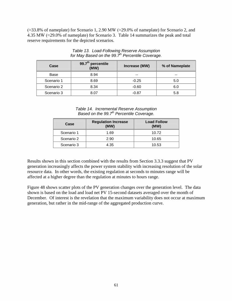
61
(≈33.8% of nameplate) for Scenario 1, 2.90 MW (≈29.0% of nameplate) for Scenario 2, and 4.35 MW (≈29.0% of nameplate) for Scenario 3. Table 14 summarizes the peak and total reserve requirements for the depicted scenarios.
Table 13. Load-Following Reserve Assumption for May Based on the 99.7th Percentile Coverage.
Case 99.7th percentile (MW) Increase (MW) % of Nameplate
Base 8.94 -- -- Scenario 1 8.69 -0.25 5.0 Scenario 2 8.34 -0.60 6.0 Scenario 3 8.07 -0.87 5.8
Table 14. Incremental Reserve Assumption Based on the 99.7th Percentile Coverage.
Case Regulation Increase (MW)
Load Follow (MW)
Scenario 1 1.69 10.72 Scenario 2 2.90 10.65 Scenario 3 4.35 10.53
Results shown in this section combined with the results from Section 3.3.3 suggest that PV generation increasingly affects the power system stability with increasing resolution of the solar resource data. In other words, the existing regulation at seconds to minutes range will be affected at a higher degree than the regulation at minutes to hours range. Figure 48 shows scatter plots of the PV generation changes over the generation level. The data shown is based on the load and load net PV 15-second datasets averaged over the month of December. Of interest is the revelation that the maximum variability does not occur at maximum generation, but rather in the mid-range of the aggregated production curve.
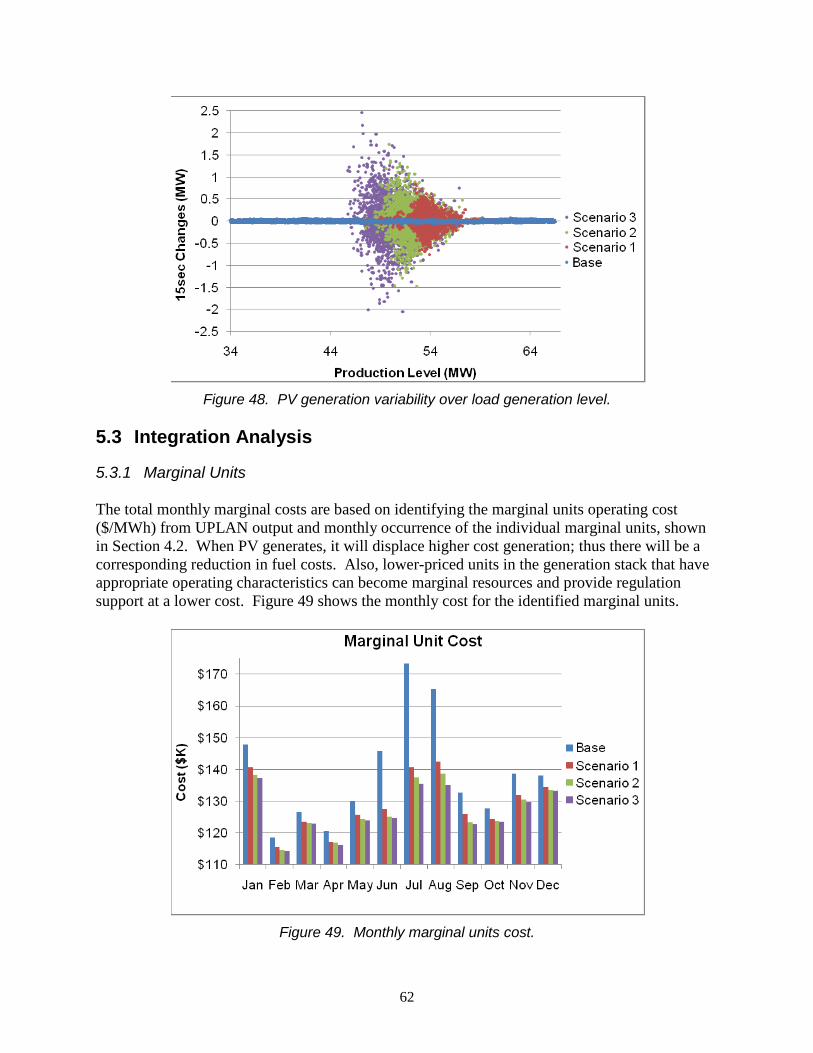
62
Figure 48. PV generation variability over load generation level.
5.3 Integration Analysis
5.3.1 Marginal Units The total monthly marginal costs are based on identifying the marginal units operating cost ($/MWh) from UPLAN output and monthly occurrence of the individual marginal units, shown in Section 4.2. When PV generates, it will displace higher cost generation; thus there will be a corresponding reduction in fuel costs. Also, lower-priced units in the generation stack that have appropriate operating characteristics can become marginal resources and provide regulation support at a lower cost. Figure 49 shows the monthly cost for the identified marginal units.
Figure 49. Monthly marginal units cost.
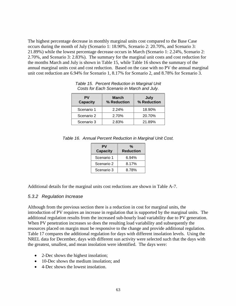
63
The highest percentage decrease in monthly marginal units cost compared to the Base Case occurs during the month of July (Scenario 1: 18.90%, Scenario 2: 20.70%, and Scenario 3: 21.89%) while the lowest percentage decrease occurs in March (Scenario 1: 2.24%, Scenario 2: 2.70%, and Scenario 3: 2.83%). The summary for the marginal unit costs and cost reduction for the months March and July is shown in Table 15, while Table 16 shows the summary of the annual marginal units cost and cost reduction. Based on the case with no PV the annual marginal unit cost reduction are 6.94% for Scenario 1, 8.17% for Scenario 2, and 8.78% for Scenario 3.
Table 15. Percent Reduction in Marginal Unit Costs for Each Scenario in March and July.
PV Capacity
March % Reduction
July % Reduction
Scenario 1 2.24% 18.90% Scenario 2 2.70% 20.70% Scenario 3 2.83% 21.89%
Table 16. Annual Percent Reduction in Marginal Unit Cost.
PV Capacity
% Reduction
Scenario 1 6.94% Scenario 2 8.17% Scenario 3 8.78%
Additional details for the marginal units cost reductions are shown in Table A-7.
5.3.2 Regulation Increase Although from the previous section there is a reduction in cost for marginal units, the introduction of PV requires an increase in regulation that is supported by the marginal units. The additional regulation results from the increased sub-hourly load variability due to PV generation. When PV penetration increases so does the resulting load variability and subsequently the resources placed on margin must be responsive to the change and provide additional regulation. Table 17 compares the additional regulation for days with different insolation levels. Using the NREL data for December, days with different sun activity were selected such that the days with the greatest, smallest, and mean insolation were identified. The days were:
• 2-Dec shows the highest insolation; • 10-Dec shows the medium insolation; and • 4-Dec shows the lowest insolation.
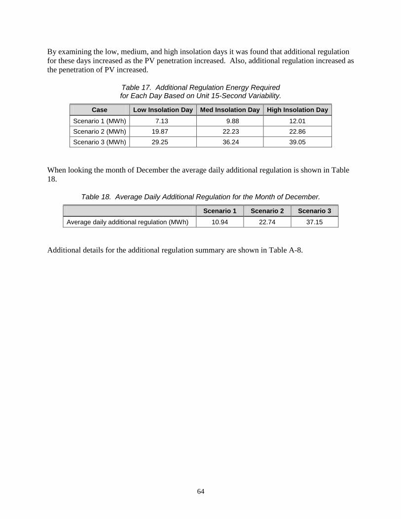
64
By examining the low, medium, and high insolation days it was found that additional regulation for these days increased as the PV penetration increased. Also, additional regulation increased as the penetration of PV increased.
Table 17. Additional Regulation Energy Required for Each Day Based on Unit 15-Second Variability.
Case Low Insolation Day Med Insolation Day High Insolation Day Scenario 1 (MWh) 7.13 9.88 12.01 Scenario 2 (MWh) 19.87 22.23 22.86 Scenario 3 (MWh) 29.25 36.24 39.05
When looking the month of December the average daily additional regulation is shown in Table 18.
Table 18. Average Daily Additional Regulation for the Month of December.
Scenario 1 Scenario 2 Scenario 3 Average daily additional regulation (MWh) 10.94 22.74 37.15
Additional details for the additional regulation summary are shown in Table A-8.
65
6 Conclusions and Findings
This section addresses findings and conclusions identified through the analysis of the PV solar resource data and the modeling of the KIUC system with 5-MW, 10-MW, and 15-MW nameplate capacity of PV generation.
• The selection of units identified as marginal resources that serve and follow system load will change. As PV generation increases, units identified as marginal resources will be units with lower operating costs. In general the cost of operations for marginal units will be reduced.
• The required spinning reserve to maintain system frequency increases with the penetration level of PV (Figure 50).
Figure 50. On-line spinning capacity requirement to
meet 99.7% of 15-second changes in net load for study scenarios.
• PV penetration will displace existing system generation, thus reducing fuel consumption. The costs of conventional generation operations are reduced due to fuel savings. However, PV energy does not come at zero cost. (The production simulations did not take into account the PV cost.)
• PV generation installed at 5-MW, 10-MW, and 15-MW penetration levels will affect regulating reserves. The study showed that as PV penetration increases the required regulating reserve to control system frequency will increase (see Table 19). These additional reserve levels would result in a frequency performance that is similar to the existing system. This analysis is based on a limited amount of high-resolution system data, and did not consider system performance during contingencies.

66
• PV penetration at any penetration level is not likely to reduce net system load. KIUC load patterns peak in the evening with a secondary peak in the morning. The peaks occur at times when PV generation is at low or zero level. PV has the best benefit for reducing system peak in the summer months when the solar day is longer.
• Increasing PV penetration has little effect on load-following reserves with negligible reduction as penetration increases (see Table 19).
Table 19. Annual Incremental Reserve Range.
Range of monthly maximum load changes for
study period in 2011
PV Penetration Base Case Scenario 1 Scenario 2 Scenario 3
From To From To From To From To Regulating (MW/15 sec) 0.10 0.34 0.95 1.69 1.66 2.90 2.25 4.35 Load-Following (MW/h) 7.45 10.79 7.30 10.72 7.23 10.65 7.07 10.53
• PV generation studies require data with time resolution less than 1 hour, preferably in seconds.
o Variability: High-resolution (1-second) solar resource data demonstrates greater variability of PV generation and can have a significant effect on system frequency. This impact may be obscured if PV generation is modeled with hourly resolution data.
o Diversity: High-resolution (1-second) solar resource data yields improved diversity between geographically separated sites. Geographical diversity has a lesser impact on variability over longer time frames.
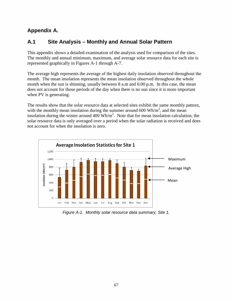
67
Appendix A. A.1 Site Analysis – Monthly and Annual Solar Pattern This appendix shows a detailed examination of the analysis used for comparison of the sites. The monthly and annual minimum, maximum, and average solar resource data for each site is represented graphically in Figures A-1 through A-7. The average high represents the average of the highest daily insolation observed throughout the month. The mean insolation represents the mean insolation observed throughout the whole month when the sun is shinning, usually between 8 a.m and 6:00 p.m. In this case, the mean does not account for those periods of the day when there is no sun since it is more important when PV is generating. The results show that the solar resource data at selected sites exhibit the same monthly pattern, with the monthly mean insolation during the summer around 600 Wh/m2, and the mean insolation during the winter around 400 Wh/m2. Note that for mean insolation calculation, the solar resource data is only averaged over a period when the solar radiation is received and does not account for when the insolation is zero.
Figure A-1. Monthly solar resource data summary, Site 1.
Maximum
Average High
Mean
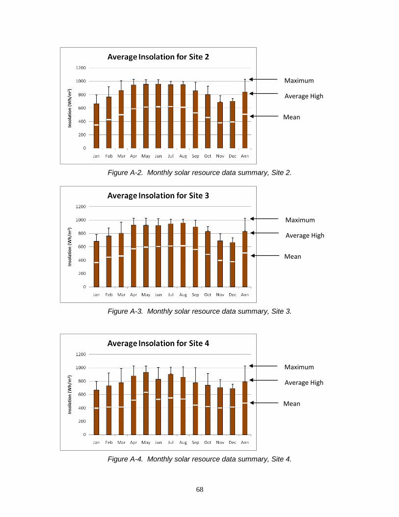
68
Figure A-2. Monthly solar resource data summary, Site 2.
Figure A-3. Monthly solar resource data summary, Site 3.
Figure A-4. Monthly solar resource data summary, Site 4.
Maximum
Average High
Mean
Maximum
Average High
Mean
Maximum
Average High
Mean
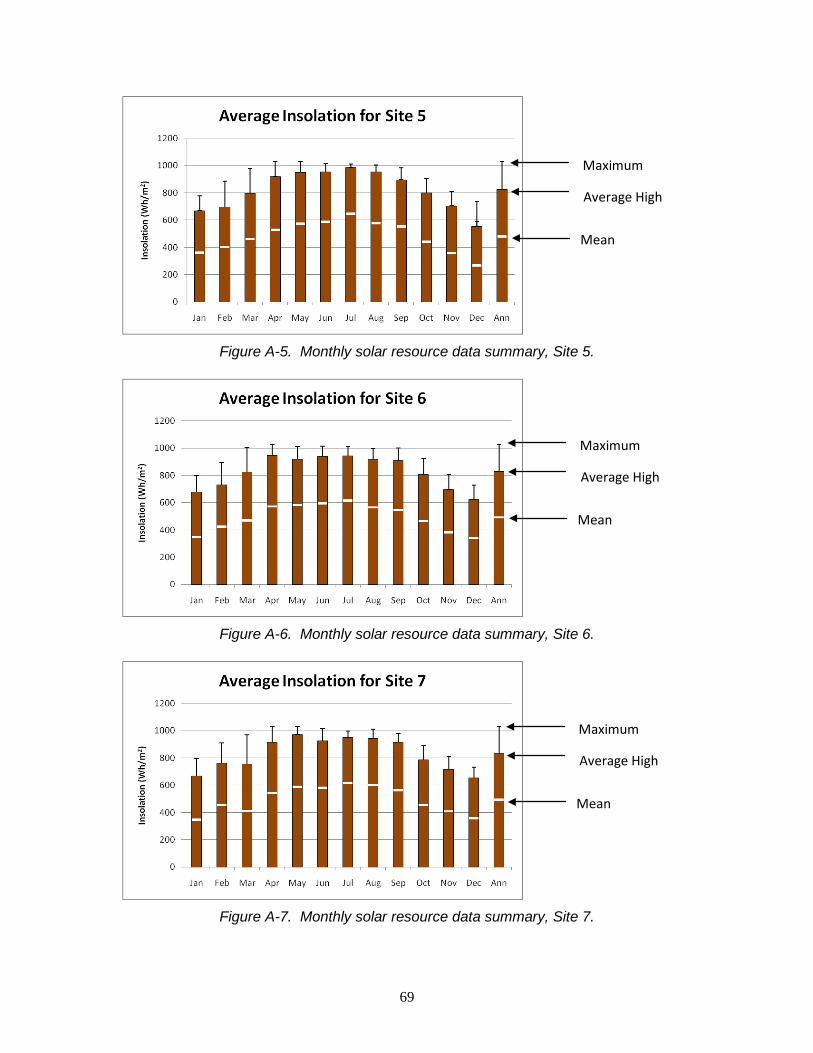
69
Figure A-5. Monthly solar resource data summary, Site 5.
Figure A-6. Monthly solar resource data summary, Site 6.
Figure A-7. Monthly solar resource data summary, Site 7.
Maximum
Average High
Mean
Maximum
Average High
Mean
Maximum
Average High
Mean

70
A.2 High-Resolution Data Modeling This section will describe the methodology used to model high-resolution solar resource data. KIUC provided 1-second solar resource data for three stations on Oahu and 2.5-minute solar resource data for Hana Kukui. The profiles provided in these data sets were used to create simulated high-resolution data from hourly profiles. First, the daily total energy was calculated for the NREL solar resource data and the high-resolution solar resource data. Each set of data was classified into four categories, as shown below. Overcast Less than or equal to 2546 kWh/M2/day Slightly Sunny Greater than Overcast and less than or equal to kWh/M2/day Moderately Sunny Greater than Slightly Sunny and less than or equal to 5960 kWh/M2/day Very Sunny Greater than Moderately Sunny Next the group of hourly data in the overcast group was randomly mapped with higher resolution data in the overcast group. The other hourly data were randomly mapped with higher-resolution data in like groups. Keeping the chronology of the data mapped with the solar resource data, the days were ranked from low to high power. The 2.5-minute data was ordered in the same way. From here the hourly data with lowest insolation day was mapped to the 2.5-minute data with lowest insolation day. Using the 2.5-minute data profile the algorithm computes the instantaneous values to obtain the variability between 2.5-minute periods while maintaining the correct hour ending average. Table A-1 shows a sample of hourly data and that data converted to 2.5-minute data. Using the same approach, the 2.5-minute solar resource data was used to create 1-second solar resource data. The 1-second solar resource data was used to generate the 15-second data used in the model described in Section 4.1.1.
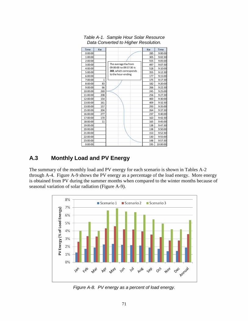
71
Table A-1. Sample Hour Solar Resource
Data Converted to Higher Resolution.
A.3 Monthly Load and PV Energy The summary of the monthly load and PV energy for each scenario is shown in Tables A-2 through A-4. Figure A-9 shows the PV energy as a percentage of the load energy. More energy is obtained from PV during the summer months when compared to the winter months because of seasonal variation of solar radiation (Figure A-9).
Figure A-8. PV energy as a percent of load energy.
Time Kw Kw Time0:00:00 285 9:00:001:00:00 305 9:02:302:00:00 555 9:05:003:00:00 497 9:07:304:00:00 518 9:10:005:00:00 355 9:12:306:00:00 177 9:15:007:00:00 1 175 9:17:308:00:00 83 182 9:20:009:00:00 66 266 9:22:30
10:00:00 269 245 9:25:0011:00:00 208 256 9:27:3012:00:00 154 400 9:30:0013:00:00 161 409 9:32:3013:00:00 157 293 9:35:0015:00:00 204 264 9:37:3016:00:00 277 237 9:40:0017:00:00 170 163 9:42:3018:00:00 11 165 9:45:0019:00:00 138 9:47:3020:00:00 138 9:50:0021:00:00 153 9:52:3022:00:00 130 9:55:0023:00:00 148 9:57:30
0:00:00 195 10:00:00
The average Kw from 09:00:00 to 09:57:30 is269, which corresponds to the hour-ending

72
Table A-2. Summary of Monthly Load and PV Energy for Scenario 1.
Load PV Scenario 1
Min
(MW) Max (MW)
Energy (GWh)
Energy (GWh)
Energy % Load
Jan 30.14 68.77 37.22 .456 1.23% Feb 27.60 62.90 31.51 .535 1.70% Mar 29.50 64.52 36.04 .677 1.88% Apr 28.87 65.44 35.10 .795 2.26% May 31.87 67.09 38.40 .898 2.34% Jun 34.29 66.73 38.29 .849 2.22% Jul 35.47 69.02 41.04 .888 2.16% Aug 36.57 70.80 42.12 .894 2.12% Sep 35.46 70.19 39.58 .744 1.88% Oct 33.14 69.81 39.63 .678 1.71% Nov 31.78 72.31 37.80 .532 1.41% Dec 30.93 71.92 38.13 .550 1.44% Annual 27.60 72.31 454.84 8.496 1.87%
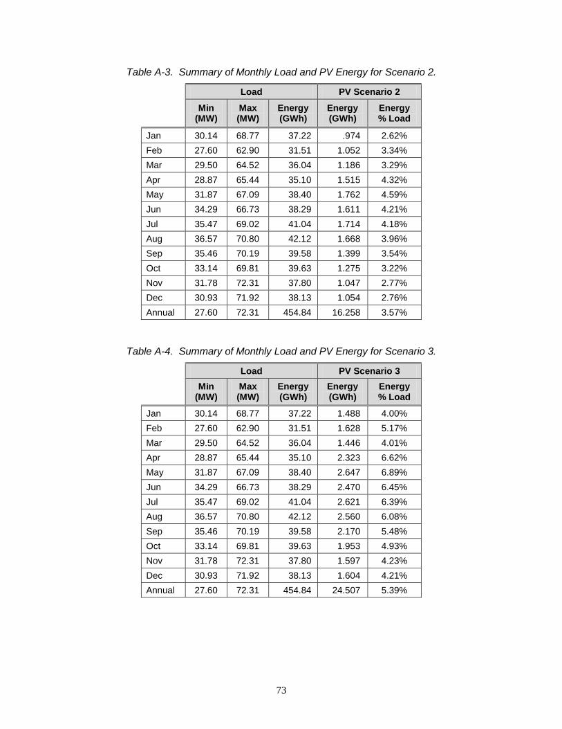
73
Table A-3. Summary of Monthly Load and PV Energy for Scenario 2.
Load PV Scenario 2
Min
(MW) Max (MW)
Energy (GWh)
Energy (GWh)
Energy % Load
Jan 30.14 68.77 37.22 .974 2.62% Feb 27.60 62.90 31.51 1.052 3.34% Mar 29.50 64.52 36.04 1.186 3.29% Apr 28.87 65.44 35.10 1.515 4.32% May 31.87 67.09 38.40 1.762 4.59% Jun 34.29 66.73 38.29 1.611 4.21% Jul 35.47 69.02 41.04 1.714 4.18% Aug 36.57 70.80 42.12 1.668 3.96% Sep 35.46 70.19 39.58 1.399 3.54% Oct 33.14 69.81 39.63 1.275 3.22% Nov 31.78 72.31 37.80 1.047 2.77% Dec 30.93 71.92 38.13 1.054 2.76% Annual 27.60 72.31 454.84 16.258 3.57%
Table A-4. Summary of Monthly Load and PV Energy for Scenario 3.
Load PV Scenario 3
Min (MW)
Max (MW)
Energy (GWh)
Energy (GWh)
Energy % Load
Jan 30.14 68.77 37.22 1.488 4.00% Feb 27.60 62.90 31.51 1.628 5.17% Mar 29.50 64.52 36.04 1.446 4.01% Apr 28.87 65.44 35.10 2.323 6.62% May 31.87 67.09 38.40 2.647 6.89% Jun 34.29 66.73 38.29 2.470 6.45% Jul 35.47 69.02 41.04 2.621 6.39% Aug 36.57 70.80 42.12 2.560 6.08% Sep 35.46 70.19 39.58 2.170 5.48% Oct 33.14 69.81 39.63 1.953 4.93% Nov 31.78 72.31 37.80 1.597 4.23% Dec 30.93 71.92 38.13 1.604 4.21% Annual 27.60 72.31 454.84 24.507 5.39%
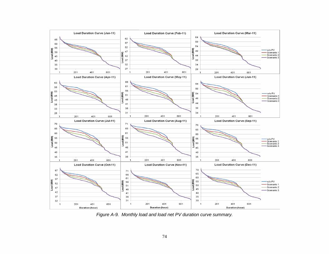
74
Figure A-9. Monthly load and load net PV duration curve summary.
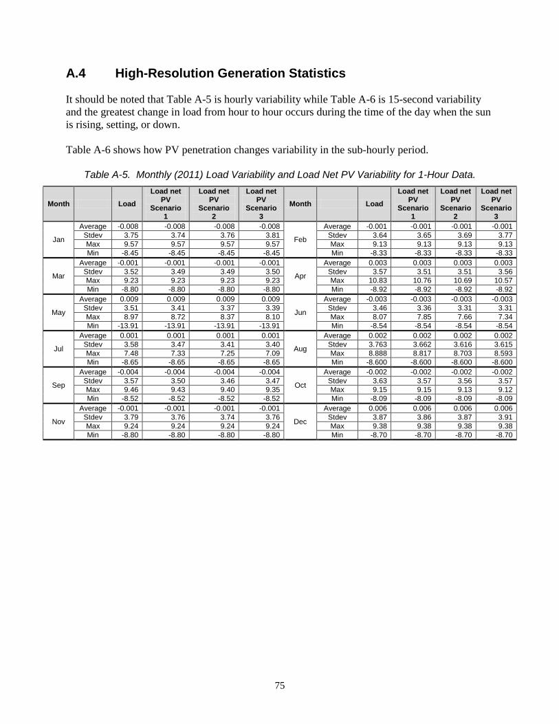
75
A.4 High-Resolution Generation Statistics It should be noted that Table A-5 is hourly variability while Table A-6 is 15-second variability and the greatest change in load from hour to hour occurs during the time of the day when the sun is rising, setting, or down. Table A-6 shows how PV penetration changes variability in the sub-hourly period.
Table A-5. Monthly (2011) Load Variability and Load Net PV Variability for 1-Hour Data.
Month Load Load net
PV Scenario
1
Load net PV
Scenario 2
Load net PV
Scenario 3
Month Load Load net
PV Scenario
1
Load net PV
Scenario 2
Load net PV
Scenario 3
Jan
Average -0.008 -0.008 -0.008 -0.008
Feb
Average -0.001 -0.001 -0.001 -0.001 Stdev 3.75 3.74 3.76 3.81 Stdev 3.64 3.65 3.69 3.77 Max 9.57 9.57 9.57 9.57 Max 9.13 9.13 9.13 9.13 Min -8.45 -8.45 -8.45 -8.45 Min -8.33 -8.33 -8.33 -8.33
Mar
Average -0.001 -0.001 -0.001 -0.001
Apr
Average 0.003 0.003 0.003 0.003 Stdev 3.52 3.49 3.49 3.50 Stdev 3.57 3.51 3.51 3.56 Max 9.23 9.23 9.23 9.23 Max 10.83 10.76 10.69 10.57 Min -8.80 -8.80 -8.80 -8.80 Min -8.92 -8.92 -8.92 -8.92
May
Average 0.009 0.009 0.009 0.009
Jun
Average -0.003 -0.003 -0.003 -0.003 Stdev 3.51 3.41 3.37 3.39 Stdev 3.46 3.36 3.31 3.31 Max 8.97 8.72 8.37 8.10 Max 8.07 7.85 7.66 7.34 Min -13.91 -13.91 -13.91 -13.91 Min -8.54 -8.54 -8.54 -8.54
Jul
Average 0.001 0.001 0.001 0.001
Aug
Average 0.002 0.002 0.002 0.002 Stdev 3.58 3.47 3.41 3.40 Stdev 3.763 3.662 3.616 3.615 Max 7.48 7.33 7.25 7.09 Max 8.888 8.817 8.703 8.593 Min -8.65 -8.65 -8.65 -8.65 Min -8.600 -8.600 -8.600 -8.600
Sep
Average -0.004 -0.004 -0.004 -0.004
Oct
Average -0.002 -0.002 -0.002 -0.002 Stdev 3.57 3.50 3.46 3.47 Stdev 3.63 3.57 3.56 3.57 Max 9.46 9.43 9.40 9.35 Max 9.15 9.15 9.13 9.12 Min -8.52 -8.52 -8.52 -8.52 Min -8.09 -8.09 -8.09 -8.09
Nov
Average -0.001 -0.001 -0.001 -0.001
Dec
Average 0.006 0.006 0.006 0.006 Stdev 3.79 3.76 3.74 3.76 Stdev 3.87 3.86 3.87 3.91 Max 9.24 9.24 9.24 9.24 Max 9.38 9.38 9.38 9.38 Min -8.80 -8.80 -8.80 -8.80 Min -8.70 -8.70 -8.70 -8.70
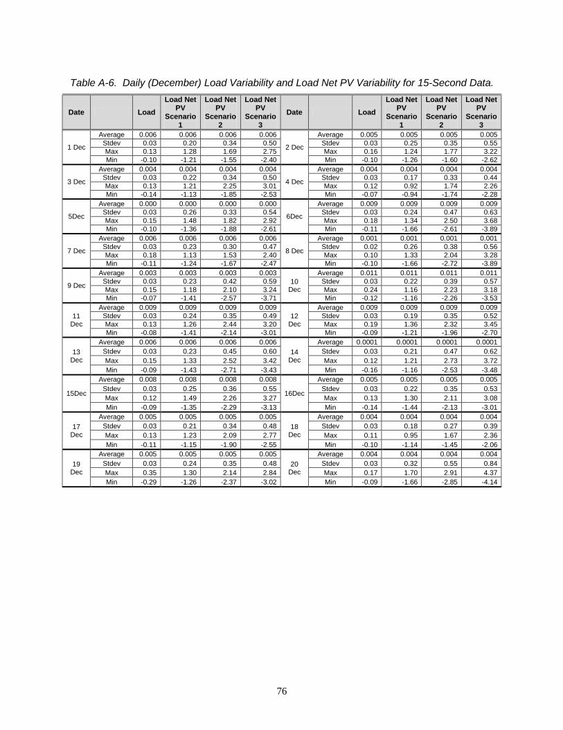
76
Table A-6. Daily (December) Load Variability and Load Net PV Variability for 15-Second Data.
Date Load Load Net
PV Scenario
1
Load Net PV
Scenario 2
Load Net PV
Scenario 3
Date Load Load Net
PV Scenario
1
Load Net PV
Scenario 2
Load Net PV
Scenario 3
1 Dec
Average 0.006 0.006 0.006 0.006
2 Dec
Average 0.005 0.005 0.005 0.005 Stdev 0.03 0.20 0.34 0.50 Stdev 0.03 0.25 0.35 0.55 Max 0.13 1.28 1.69 2.75 Max 0.16 1.24 1.77 3.22 Min -0.10 -1.21 -1.55 -2.40 Min -0.10 -1.26 -1.60 -2.62
3 Dec
Average 0.004 0.004 0.004 0.004
4 Dec
Average 0.004 0.004 0.004 0.004 Stdev 0.03 0.22 0.34 0.50 Stdev 0.03 0.17 0.33 0.44 Max 0.13 1.21 2.25 3.01 Max 0.12 0.92 1.74 2.26 Min -0.14 -1.13 -1.85 -2.53 Min -0.07 -0.94 -1.74 -2.28
5Dec
Average 0.000 0.000 0.000 0.000
6Dec
Average 0.009 0.009 0.009 0.009 Stdev 0.03 0.26 0.33 0.54 Stdev 0.03 0.24 0.47 0.63 Max 0.15 1.48 1.82 2.92 Max 0.18 1.34 2.50 3.68 Min -0.10 -1.36 -1.88 -2.61 Min -0.11 -1.66 -2.61 -3.89
7 Dec
Average 0.006 0.006 0.006 0.006
8 Dec
Average 0.001 0.001 0.001 0.001 Stdev 0.03 0.23 0.30 0.47 Stdev 0.02 0.26 0.38 0.56 Max 0.18 1.13 1.53 2.40 Max 0.10 1.33 2.04 3.28 Min -0.11 -1.24 -1.67 -2.47 Min -0.10 -1.66 -2.72 -3.89
9 Dec
Average 0.003 0.003 0.003 0.003 10
Dec
Average 0.011 0.011 0.011 0.011 Stdev 0.03 0.23 0.42 0.59 Stdev 0.03 0.22 0.39 0.57 Max 0.15 1.18 2.10 3.24 Max 0.24 1.16 2.23 3.18 Min -0.07 -1.41 -2.57 -3.71 Min -0.12 -1.16 -2.26 -3.53
11 Dec
Average 0.009 0.009 0.009 0.009 12
Dec
Average 0.009 0.009 0.009 0.009 Stdev 0.03 0.24 0.35 0.49 Stdev 0.03 0.19 0.35 0.52 Max 0.13 1.26 2.44 3.20 Max 0.19 1.36 2.32 3.45 Min -0.08 -1.41 -2.14 -3.01 Min -0.09 -1.21 -1.96 -2.70
13 Dec
Average 0.006 0.006 0.006 0.006 14
Dec
Average 0.0001 0.0001 0.0001 0.0001 Stdev 0.03 0.23 0.45 0.60 Stdev 0.03 0.21 0.47 0.62 Max 0.15 1.33 2.52 3.42 Max 0.12 1.21 2.73 3.72 Min -0.09 -1.43 -2.71 -3.43 Min -0.16 -1.16 -2.53 -3.48
15Dec
Average 0.008 0.008 0.008 0.008
16Dec
Average 0.005 0.005 0.005 0.005 Stdev 0.03 0.25 0.36 0.55 Stdev 0.03 0.22 0.35 0.53 Max 0.12 1.49 2.26 3.27 Max 0.13 1.30 2.11 3.08 Min -0.09 -1.35 -2.29 -3.13 Min -0.14 -1.44 -2.13 -3.01
17 Dec
Average 0.005 0.005 0.005 0.005 18
Dec
Average 0.004 0.004 0.004 0.004 Stdev 0.03 0.21 0.34 0.48 Stdev 0.03 0.18 0.27 0.39 Max 0.13 1.23 2.09 2.77 Max 0.11 0.95 1.67 2.36 Min -0.11 -1.15 -1.90 -2.55 Min -0.10 -1.14 -1.45 -2.06
19 Dec
Average 0.005 0.005 0.005 0.005 20
Dec
Average 0.004 0.004 0.004 0.004 Stdev 0.03 0.24 0.35 0.48 Stdev 0.03 0.32 0.55 0.84 Max 0.35 1.30 2.14 2.84 Max 0.17 1.70 2.91 4.37 Min -0.29 -1.26 -2.37 -3.02 Min -0.09 -1.66 -2.85 -4.14
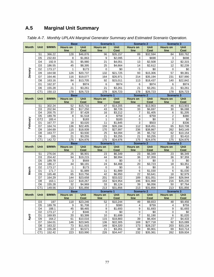
77
A.5 Marginal Unit Summary Table A-7. Monthly UPLAN Marginal Generator Summary and Estimated Scenario Operation.
Month Unit $/MWh Base Scenario 1 Scenario 2 Scenario 3
Hours on line
Unit Cost
Hours on line
Unit Cost
Hours on line
Unit Cost
Hours on line
Unit Cost
Janu
ary
S1 366.22 128 $46,876 96 $35,157 89 $32,594 84 $30,762 D5 232.83 8 $1,863 9 $2,095 3 $698 3 $698 D4 192.9 31 $5,980 21 $4,051 13 $2,508 12 $2,315 D3 186.55 45 $8,395 25 $4,664 14 $2,612 12 $2,239 D2 173.17 1 $173 0 $0 0 $0 0 $0 D9 164.58 126 $20,737 132 $21,725 93 $15,306 57 $9,381 D7 164.46 116 $19,077 164 $26,971 214 $35,194 231 $37,990 D8 163.16 84 $13,705 92 $15,011 113 $18,437 140 $22,842 D1 162.37 6 $974 6 $974 6 $974 6 $974 D6 155.28 21 $3,261 21 $3,261 21 $3,261 21 $3,261
CT1 150.13 178 $26,723 178 $26,723 178 $26,723 178 $26,723
Month Unit $/MWh Base Scenario 1 Scenario 2 Scenario 3
Hours on line
Unit Cost
Hours on line
Unit Cost
Hours on line
Unit Cost
Hours on line
Unit Cost
Febr
uary
S1 302.24 52 $15,716 47 $14,205 46 $13,903 46 $13,903 D3 202.94 85 $17,250 43 $8,726 33 $6,697 30 $6,088 D4 200.75 37 $7,428 16 $3,212 7 $1,405 6 $1,205 D5 189.78 8 $1,518 4 $759 4 $759 2 $380
GT2 183.4 1 $183 1 $183 0 $0 0 $0 D1 167.77 18 $3,020 11 $1,845 3 $503 2 $336 D7 164.74 136 $22,405 159 $26,194 112 $18,451 65 $10,708 D9 164.69 115 $18,939 170 $27,997 236 $38,867 262 $43,149 D8 163.77 24 $3,930 25 $4,094 35 $5,732 62 $10,154 D6 155 21 $3,255 21 $3,255 21 $3,255 22 $3,410
CT1 142.72 175 $24,976 175 $24,976 175 $24,976 175 $24,976
Month Unit $/MWh Base Scenario 1 Scenario 2 Scenario 3
Hours on line
Unit Cost
Hours on line
Unit Cost
Hours on line
Unit Cost
Hours on line
Unit Cost
Mar
ch
S1 276.04 25 $6,901 23 $6,349 23 $6,349 23 $6,349 D3 204.42 94 $19,215 44 $8,994 36 $7,359 36 $7,359 D5 189.78 3 $569 0 $0 0 $0 0 $0 D4 186.17 44 $8,191 24 $4,468 20 $3,723 18 $3,351 D2 173.17 1 $173 0 $0 0 $0 0 $0 D1 171.7 11 $1,889 11 $1,889 6 $1,030 6 $1,030 D9 165.48 65 $10,756 42 $6,950 22 $3,641 18 $2,979 D7 164.29 144 $23,658 201 $33,022 189 $31,051 164 $26,944 D8 163.1 112 $18,267 153 $24,954 196 $31,968 216 $35,230 D6 155.28 32 $4,969 33 $5,124 39 $6,056 50 $7,764
CT1 149.56 213 $31,856 213 $31,856 213 $31,856 213 $31,856
Month Unit $/MWh Base Scenario 1 Scenario 2 Scenario 3
Hours on line
Unit Cost
Hours on line
Unit Cost
Hours on line
Unit Cost
Hours on line
Unit Cost
Apr
il
D3 197 118 $23,246 52 $10,244 49 $9,653 48 $9,456 D5 189.78 9 $1,708 2 $380 4 $759 4 $759 D4 188.1 45 $8,465 9 $1,693 9 $1,693 9 $1,693 D2 173.17 2 $346 0 $0 0 $0 0 $0 D1 169.93 20 $3,399 10 $1,699 7 $1,190 6 $1,020 D9 164.2 61 $10,016 115 $18,883 39 $6,404 27 $4,433 D7 164.01 146 $23,945 136 $22,305 169 $27,718 92 $15,089 D8 163.22 73 $11,915 149 $24,320 173 $28,237 203 $33,134 D6 155.28 23 $3,571 21 $3,261 38 $5,901 69 $10,714
CT1 152.42 223 $33,990 226 $34,447 232 $35,361 262 $39,934
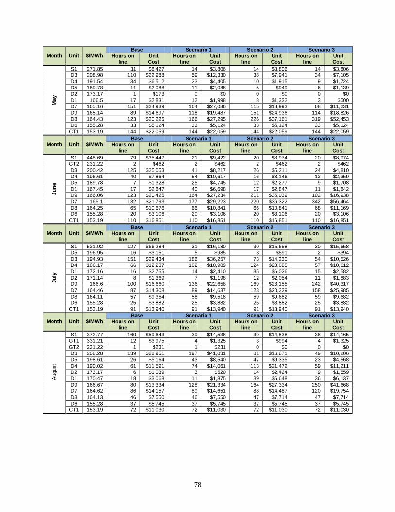
78
Month Unit $/MWh Base Scenario 1 Scenario 2 Scenario 3
Hours on line
Unit Cost
Hours on line
Unit Cost
Hours on line
Unit Cost
Hours on line
Unit Cost
May
S1 271.85 31 $8,427 14 $3,806 14 $3,806 14 $3,806 D3 208.98 110 $22,988 59 $12,330 38 $7,941 34 $7,105 D4 191.54 34 $6,512 23 $4,405 10 $1,915 9 $1,724 D5 189.78 11 $2,088 11 $2,088 5 $949 6 $1,139 D2 173.17 1 $173 0 $0 0 $0 0 $0 D1 166.5 17 $2,831 12 $1,998 8 $1,332 3 $500 D7 165.16 151 $24,939 164 $27,086 115 $18,993 68 $11,231 D9 165.14 89 $14,697 118 $19,487 151 $24,936 114 $18,826 D8 164.43 123 $20,225 166 $27,295 226 $37,161 319 $52,453 D6 155.28 33 $5,124 33 $5,124 33 $5,124 33 $5,124
CT1 153.19 144 $22,059 144 $22,059 144 $22,059 144 $22,059
Month Unit $/MWh Base Scenario 1 Scenario 2 Scenario 3
Hours on line
Unit Cost
Hours on line
Unit Cost
Hours on line
Unit Cost
Hours on line
Unit Cost
June
S1 448.69 79 $35,447 21 $9,422 20 $8,974 20 $8,974 GT2 231.22 2 $462 2 $462 2 $462 2 $462 D3 200.42 125 $25,053 41 $8,217 26 $5,211 24 $4,810 D4 196.61 40 $7,864 54 $10,617 16 $3,146 12 $2,359 D5 189.78 7 $1,328 25 $4,745 12 $2,277 9 $1,708 D1 167.45 17 $2,847 40 $6,698 17 $2,847 11 $1,842 D9 166.06 123 $20,425 164 $27,234 211 $35,039 102 $16,938 D7 165.1 132 $21,793 177 $29,223 220 $36,322 342 $56,464 D8 164.25 65 $10,676 66 $10,841 66 $10,841 68 $11,169 D6 155.28 20 $3,106 20 $3,106 20 $3,106 20 $3,106
CT1 153.19 110 $16,851 110 $16,851 110 $16,851 110 $16,851
Month Unit $/MWh Base Scenario 1 Scenario 2 Scenario 3
Hours on line
Unit Cost
Hours on line
Unit Cost
Hours on line
Unit Cost
Hours on line
Unit Cost
July
S1 521.92 127 $66,284 31 $16,180 30 $15,658 30 $15,658 D5 196.95 16 $3,151 5 $985 3 $591 2 $394 D3 194.93 151 $29,434 186 $36,257 73 $14,230 54 $10,526 D4 186.17 66 $12,287 102 $18,989 124 $23,085 57 $10,612 D1 172.16 16 $2,755 14 $2,410 35 $6,026 15 $2,582 D2 171.14 8 $1,369 7 $1,198 12 $2,054 11 $1,883 D9 166.6 100 $16,660 136 $22,658 169 $28,155 242 $40,317 D7 164.46 87 $14,308 89 $14,637 123 $20,229 158 $25,985 D8 164.11 57 $9,354 58 $9,518 59 $9,682 59 $9,682 D6 155.28 25 $3,882 25 $3,882 25 $3,882 25 $3,882
CT1 153.19 91 $13,940 91 $13,940 91 $13,940 91 $13,940
Month Unit $/MWh Base Scenario 1 Scenario 2 Scenario 3
Hours on line
Unit Cost
Hours on line
Unit Cost
Hours on line
Unit Cost
Hours on line
Unit Cost
Aug
ust
S1 372.77 160 $59,643 39 $14,538 39 $14,538 38 $14,165 GT1 331.21 12 $3,975 4 $1,325 3 $994 4 $1,325 GT2 231.22 1 $231 1 $231 0 $0 0 $0 D3 208.28 139 $28,951 197 $41,031 81 $16,871 49 $10,206 D5 198.61 26 $5,164 43 $8,540 47 $9,335 23 $4,568 D4 190.02 61 $11,591 74 $14,061 113 $21,472 59 $11,211 D2 173.17 6 $1,039 3 $520 14 $2,424 9 $1,559 D1 170.47 18 $3,068 11 $1,875 39 $6,648 36 $6,137 D9 166.67 80 $13,334 128 $21,334 164 $27,334 250 $41,668 D7 164.62 86 $14,157 89 $14,651 88 $14,487 120 $19,754 D8 164.13 46 $7,550 46 $7,550 47 $7,714 47 $7,714 D6 155.28 37 $5,745 37 $5,745 37 $5,745 37 $5,745
CT1 153.19 72 $11,030 72 $11,030 72 $11,030 72 $11,030
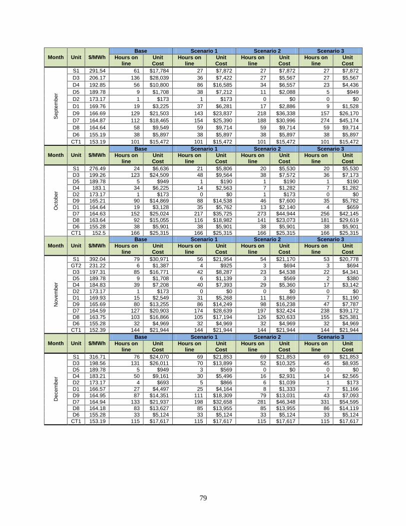
79
Month Unit $/MWh Base Scenario 1 Scenario 2 Scenario 3
Hours on line
Unit Cost
Hours on line
Unit Cost
Hours on line
Unit Cost
Hours on line
Unit Cost
Sep
tem
ber
S1 291.54 61 $17,784 27 $7,872 27 $7,872 27 $7,872 D3 206.17 136 $28,039 36 $7,422 27 $5,567 27 $5,567 D4 192.85 56 $10,800 86 $16,585 34 $6,557 23 $4,436 D5 189.78 9 $1,708 38 $7,212 11 $2,088 5 $949 D2 173.17 1 $173 1 $173 0 $0 0 $0 D1 169.76 19 $3,225 37 $6,281 17 $2,886 9 $1,528 D9 166.69 129 $21,503 143 $23,837 218 $36,338 157 $26,170 D7 164.87 112 $18,465 154 $25,390 188 $30,996 274 $45,174 D8 164.64 58 $9,549 59 $9,714 59 $9,714 59 $9,714 D6 155.19 38 $5,897 38 $5,897 38 $5,897 38 $5,897
CT1 153.19 101 $15,472 101 $15,472 101 $15,472 101 $15,472
Month Unit $/MWh Base Scenario 1 Scenario 2 Scenario 3
Hours on line
Unit Cost
Hours on line
Unit Cost
Hours on line
Unit Cost
Hours on line
Unit Cost
Oct
ober
S1 276.49 24 $6,636 21 $5,806 20 $5,530 20 $5,530 D3 199.26 123 $24,509 48 $9,564 38 $7,572 36 $7,173 D5 189.78 5 $949 1 $190 1 $190 1 $190 D4 183.1 34 $6,225 14 $2,563 7 $1,282 7 $1,282 D2 173.17 1 $173 0 $0 1 $173 0 $0 D9 165.21 90 $14,869 88 $14,538 46 $7,600 35 $5,782 D1 164.64 19 $3,128 35 $5,762 13 $2,140 4 $659 D7 164.63 152 $25,024 217 $35,725 273 $44,944 256 $42,145 D8 163.64 92 $15,055 116 $18,982 141 $23,073 181 $29,619 D6 155.28 38 $5,901 38 $5,901 38 $5,901 38 $5,901
CT1 152.5 166 $25,315 166 $25,315 166 $25,315 166 $25,315
Month Unit $/MWh Base Scenario 1 Scenario 2 Scenario 3
Hours on line
Unit Cost
Hours on line
Unit Cost
Hours on line
Unit Cost
Hours on line
Unit Cost
Nov
embe
r
S1 392.04 79 $30,971 56 $21,954 54 $21,170 53 $20,778 GT2 231.22 6 $1,387 4 $925 3 $694 3 $694 D3 197.31 85 $16,771 42 $8,287 23 $4,538 22 $4,341 D5 189.78 9 $1,708 6 $1,139 3 $569 2 $380 D4 184.83 39 $7,208 40 $7,393 29 $5,360 17 $3,142 D2 173.17 1 $173 0 $0 0 $0 0 $0 D1 169.93 15 $2,549 31 $5,268 11 $1,869 7 $1,190 D9 165.69 80 $13,255 86 $14,249 98 $16,238 47 $7,787 D7 164.59 127 $20,903 174 $28,639 197 $32,424 238 $39,172 D8 163.75 103 $16,866 105 $17,194 126 $20,633 155 $25,381 D6 155.28 32 $4,969 32 $4,969 32 $4,969 32 $4,969
CT1 152.39 144 $21,944 144 $21,944 144 $21,944 144 $21,944
Month Unit $/MWh Base Scenario 1 Scenario 2 Scenario 3
Hours on line
Unit Cost
Hours on line
Unit Cost
Hours on line
Unit Cost
Hours on line
Unit Cost
Dec
embe
r
S1 316.71 76 $24,070 69 $21,853 69 $21,853 69 $21,853 D3 198.56 131 $26,011 70 $13,899 52 $10,325 45 $8,935 D5 189.78 5 $949 3 $569 0 $0 0 $0 D4 183.21 50 $9,161 30 $5,496 16 $2,931 14 $2,565 D2 173.17 4 $693 5 $866 6 $1,039 1 $173 D1 166.57 27 $4,497 25 $4,164 8 $1,333 7 $1,166 D9 164.95 87 $14,351 111 $18,309 79 $13,031 43 $7,093 D7 164.94 133 $21,937 198 $32,658 281 $46,348 331 $54,595 D8 164.18 83 $13,627 85 $13,955 85 $13,955 86 $14,119 D6 155.28 33 $5,124 33 $5,124 33 $5,124 33 $5,124
CT1 153.19 115 $17,617 115 $17,617 115 $17,617 115 $17,617
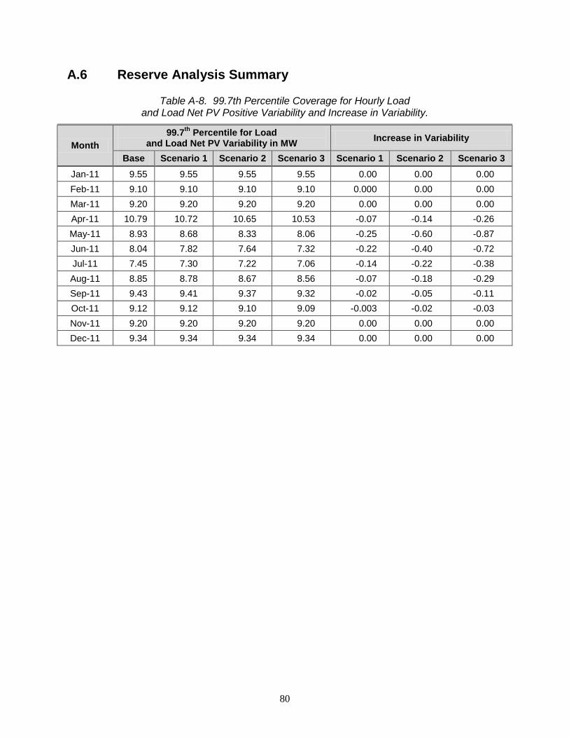
80
A.6 Reserve Analysis Summary
Table A-8. 99.7th Percentile Coverage for Hourly Load and Load Net PV Positive Variability and Increase in Variability.
Month 99.7th Percentile for Load
and Load Net PV Variability in MW Increase in Variability
Base Scenario 1 Scenario 2 Scenario 3 Scenario 1 Scenario 2 Scenario 3 Jan-11 9.55 9.55 9.55 9.55 0.00 0.00 0.00 Feb-11 9.10 9.10 9.10 9.10 0.000 0.00 0.00 Mar-11 9.20 9.20 9.20 9.20 0.00 0.00 0.00 Apr-11 10.79 10.72 10.65 10.53 -0.07 -0.14 -0.26 May-11 8.93 8.68 8.33 8.06 -0.25 -0.60 -0.87 Jun-11 8.04 7.82 7.64 7.32 -0.22 -0.40 -0.72 Jul-11 7.45 7.30 7.22 7.06 -0.14 -0.22 -0.38 Aug-11 8.85 8.78 8.67 8.56 -0.07 -0.18 -0.29 Sep-11 9.43 9.41 9.37 9.32 -0.02 -0.05 -0.11 Oct-11 9.12 9.12 9.10 9.09 -0.003 -0.02 -0.03 Nov-11 9.20 9.20 9.20 9.20 0.00 0.00 0.00 Dec-11 9.34 9.34 9.34 9.34 0.00 0.00 0.00
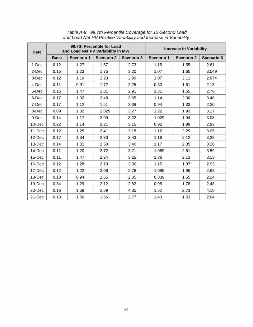
81
Table A-9. 99.7th Percentile Coverage for 15-Second Load and Load Net PV Positive Variability and Increase in Variability.
Date 99.7th Percentile for Load
and Load Net PV Variability in MW Increase in Variability
Base Scenario 1 Scenario 2 Scenario 3 Scenario 1 Scenario 2 Scenario 3 1-Dec 0.12 1.27 1.67 2.73 1.15 1.55 2.61 2-Dec 0.15 1.23 1.75 3.20 1.07 1.60 3.049 3-Dec 0.12 1.19 2.23 2.99 1.07 2.11 2.874 4-Dec 0.11 0.91 1.72 2.25 0.80 1.61 2.13 5-Dec 0.15 1.47 1.81 2.91 1.31 1.65 2.76 6-Dec 0.17 1.32 2.48 3.65 1.14 2.30 3.48 7-Dec 0.17 1.12 1.51 2.38 0.94 1.33 2.20 8-Dec 0.09 1.32 2.029 3.27 1.22 1.93 3.17 9-Dec 0.14 1.17 2.09 3.22 1.029 1.94 3.08 10-Dec 0.22 1.14 2.21 3.15 0.92 1.99 2.93 11-Dec 0.12 1.25 2.41 3.18 1.12 2.29 3.05 12-Dec 0.17 1.34 2.30 3.43 1.16 2.12 3.25 13-Dec 0.14 1.31 2.50 3.40 1.17 2.35 3.26 14-Dec 0.11 1.20 2.72 3.71 1.089 2.61 3.59 15-Dec 0.11 1.47 2.24 3.25 1.36 2.13 3.13 16-Dec 0.12 1.28 2.10 3.06 1.15 1.97 2.93 17-Dec 0.12 1.22 2.08 2.76 1.095 1.95 2.63 18-Dec 0.10 0.94 1.65 2.35 0.839 1.55 2.24 19-Dec 0.34 1.29 2.12 2.82 0.95 1.78 2.48 20-Dec 0.16 1.69 2.89 4.35 1.52 2.73 4.18 21-Dec 0.13 1.56 1.66 2.77 1.43 1.53 2.64
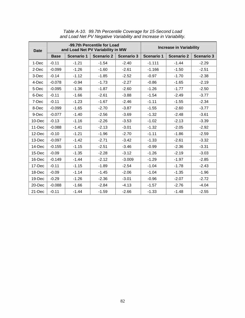
82
Table A-10. 99.7th Percentile Coverage for 15-Second Load and Load Net PV Negative Variability and Increase in Variability.
Date -99.7th Percentile for Load
and Load Net PV Variability in MW Increase in Variability
Base Scenario 1 Scenario 2 Scenario 3 Scenario 1 Scenario 2 Scenario 3 1-Dec -0.11 -1.21 -1.54 -2.40 -1.111 -1.44 -2.29 2-Dec -0.099 -1.26 -1.60 -2.61 -1.166 -1.50 -2.51 3-Dec -0.14 -1.12 -1.85 -2.52 -0.97 -1.70 -2.38 4-Dec -0.078 -0.94 -1.73 -2.27 -0.86 -1.65 -2.19 5-Dec -0.095 -1.36 -1.87 -2.60 -1.26 -1.77 -2.50 6-Dec -0.11 -1.66 -2.61 -3.88 -1.54 -2.49 -3.77 7-Dec -0.11 -1.23 -1.67 -2.46 -1.11 -1.55 -2.34 8-Dec -0.099 -1.65 -2.70 -3.87 -1.55 -2.60 -3.77 9-Dec -0.077 -1.40 -2.56 -3.69 -1.32 -2.48 -3.61
10-Dec -0.13 -1.16 -2.26 -3.53 -1.02 -2.13 -3.39 11-Dec -0.088 -1.41 -2.13 -3.01 -1.32 -2.05 -2.92 12-Dec -0.10 -1.21 -1.96 -2.70 -1.11 -1.86 -2.59 13-Dec -0.097 -1.42 -2.71 -3.42 -1.33 -2.61 -3.32 14-Dec -0.155 -1.15 -2.51 -3.46 -0.99 -2.36 -3.31 15-Dec -0.09 -1.35 -2.28 -3.12 -1.26 -2.19 -3.03 16-Dec -0.149 -1.44 -2.12 -3.009 -1.29 -1.97 -2.85 17-Dec -0.11 -1.15 -1.89 -2.54 -1.04 -1.78 -2.43 18-Dec -0.09 -1.14 -1.45 -2.06 -1.04 -1.35 -1.96 19-Dec -0.29 -1.26 -2.36 -3.01 -0.96 -2.07 -2.72 20-Dec -0.088 -1.66 -2.84 -4.13 -1.57 -2.76 -4.04 21-Dec -0.11 -1.44 -1.59 -2.66 -1.33 -1.48 -2.55
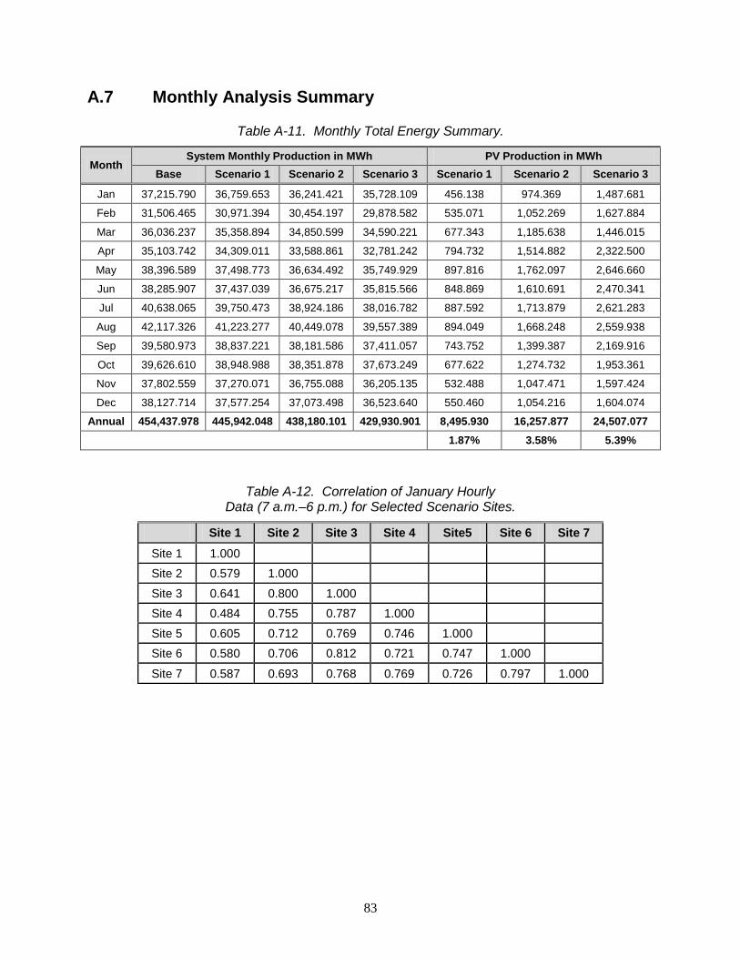
83
A.7 Monthly Analysis Summary
Table A-11. Monthly Total Energy Summary.
Month System Monthly Production in MWh PV Production in MWh
Base Scenario 1 Scenario 2 Scenario 3 Scenario 1 Scenario 2 Scenario 3
Jan 37,215.790 36,759.653 36,241.421 35,728.109 456.138 974.369 1,487.681
Feb 31,506.465 30,971.394 30,454.197 29,878.582 535.071 1,052.269 1,627.884
Mar 36,036.237 35,358.894 34,850.599 34,590.221 677.343 1,185.638 1,446.015
Apr 35,103.742 34,309.011 33,588.861 32,781.242 794.732 1,514.882 2,322.500
May 38,396.589 37,498.773 36,634.492 35,749.929 897.816 1,762.097 2,646.660
Jun 38,285.907 37,437.039 36,675.217 35,815.566 848.869 1,610.691 2,470.341
Jul 40,638.065 39,750.473 38,924.186 38,016.782 887.592 1,713.879 2,621.283
Aug 42,117.326 41,223.277 40,449.078 39,557.389 894.049 1,668.248 2,559.938
Sep 39,580.973 38,837.221 38,181.586 37,411.057 743.752 1,399.387 2,169.916
Oct 39,626.610 38,948.988 38,351.878 37,673.249 677.622 1,274.732 1,953.361
Nov 37,802.559 37,270.071 36,755.088 36,205.135 532.488 1,047.471 1,597.424
Dec 38,127.714 37,577.254 37,073.498 36,523.640 550.460 1,054.216 1,604.074 Annual 454,437.978 445,942.048 438,180.101 429,930.901 8,495.930 16,257.877 24,507.077
1.87% 3.58% 5.39%
Table A-12. Correlation of January Hourly Data (7 a.m.–6 p.m.) for Selected Scenario Sites.
Site 1 Site 2 Site 3 Site 4 Site5 Site 6 Site 7 Site 1 1.000
Site 2 0.579 1.000 Site 3 0.641 0.800 1.000
Site 4 0.484 0.755 0.787 1.000 Site 5 0.605 0.712 0.769 0.746 1.000
Site 6 0.580 0.706 0.812 0.721 0.747 1.000 Site 7 0.587 0.693 0.768 0.769 0.726 0.797 1.000
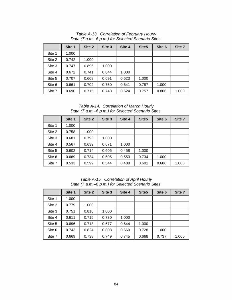
84
Table A-13. Correlation of February Hourly
Data (7 a.m.–6 p.m.) for Selected Scenario Sites.
Site 1 Site 2 Site 3 Site 4 Site5 Site 6 Site 7 Site 1 1.000
Site 2 0.742 1.000 Site 3 0.747 0.895 1.000
Site 4 0.672 0.741 0.844 1.000 Site 5 0.707 0.668 0.691 0.623 1.000
Site 6 0.661 0.702 0.750 0.641 0.787 1.000 Site 7 0.690 0.715 0.743 0.624 0.757 0.806 1.000
Table A-14. Correlation of March Hourly Data (7 a.m.–6 p.m.) for Selected Scenario Sites.
Site 1 Site 2 Site 3 Site 4 Site5 Site 6 Site 7 Site 1 1.000
Site 2 0.758 1.000 Site 3 0.681 0.793 1.000
Site 4 0.567 0.639 0.671 1.000 Site 5 0.602 0.714 0.605 0.458 1.000
Site 6 0.669 0.734 0.605 0.553 0.734 1.000 Site 7 0.533 0.599 0.544 0.488 0.601 0.686 1.000
Table A-15. Correlation of April Hourly Data (7 a.m.–6 p.m.) for Selected Scenario Sites.
Site 1 Site 2 Site 3 Site 4 Site5 Site 6 Site 7 Site 1 1.000
Site 2 0.779 1.000 Site 3 0.751 0.816 1.000
Site 4 0.611 0.715 0.730 1.000 Site 5 0.696 0.718 0.677 0.644 1.000
Site 6 0.743 0.824 0.808 0.669 0.728 1.000 Site 7 0.669 0.738 0.749 0.745 0.668 0.737 1.000
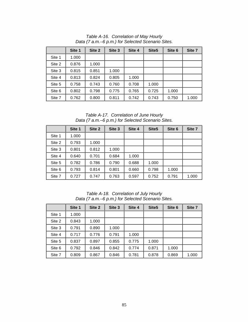
85
Table A-16. Correlation of May Hourly
Data (7 a.m.–6 p.m.) for Selected Scenario Sites.
Site 1 Site 2 Site 3 Site 4 Site5 Site 6 Site 7 Site 1 1.000
Site 2 0.876 1.000 Site 3 0.815 0.851 1.000
Site 4 0.813 0.824 0.805 1.000 Site 5 0.758 0.743 0.760 0.708 1.000
Site 6 0.802 0.798 0.775 0.765 0.725 1.000 Site 7 0.762 0.800 0.811 0.742 0.743 0.750 1.000
Table A-17. Correlation of June Hourly Data (7 a.m.–6 p.m.) for Selected Scenario Sites.
Site 1 Site 2 Site 3 Site 4 Site5 Site 6 Site 7 Site 1 1.000
Site 2 0.793 1.000 Site 3 0.801 0.812 1.000
Site 4 0.640 0.701 0.684 1.000 Site 5 0.782 0.786 0.790 0.688 1.000
Site 6 0.793 0.814 0.801 0.660 0.798 1.000 Site 7 0.727 0.747 0.763 0.597 0.752 0.791 1.000
Table A-18. Correlation of July Hourly Data (7 a.m.–6 p.m.) for Selected Scenario Sites.
Site 1 Site 2 Site 3 Site 4 Site5 Site 6 Site 7 Site 1 1.000
Site 2 0.843 1.000 Site 3 0.791 0.890 1.000
Site 4 0.717 0.776 0.791 1.000 Site 5 0.837 0.897 0.855 0.775 1.000
Site 6 0.792 0.846 0.842 0.774 0.871 1.000 Site 7 0.809 0.867 0.846 0.781 0.878 0.869 1.000
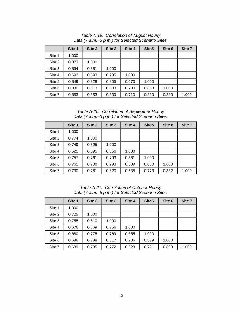
86
Table A-19. Correlation of August Hourly
Data (7 a.m.–6 p.m.) for Selected Scenario Sites.
Site 1 Site 2 Site 3 Site 4 Site5 Site 6 Site 7 Site 1 1.000
Site 2 0.873 1.000 Site 3 0.854 0.881 1.000
Site 4 0.692 0.693 0.735 1.000 Site 5 0.849 0.828 0.805 0.670 1.000
Site 6 0.830 0.813 0.803 0.700 0.853 1.000 Site 7 0.853 0.853 0.839 0.710 0.830 0.830 1.000
Table A-20. Correlation of September Hourly Data (7 a.m.–6 p.m.) for Selected Scenario Sites.
Site 1 Site 2 Site 3 Site 4 Site5 Site 6 Site 7 Site 1 1.000
Site 2 0.774 1.000 Site 3 0.749 0.825 1.000
Site 4 0.521 0.595 0.656 1.000 Site 5 0.757 0.761 0.793 0.561 1.000
Site 6 0.761 0.780 0.793 0.589 0.830 1.000 Site 7 0.730 0.781 0.820 0.635 0.773 0.832 1.000
Table A-21. Correlation of October Hourly Data (7 a.m.–6 p.m.) for Selected Scenario Sites.
Site 1 Site 2 Site 3 Site 4 Site5 Site 6 Site 7 Site 1 1.000
Site 2 0.725 1.000 Site 3 0.755 0.810 1.000
Site 4 0.676 0.669 0.756 1.000 Site 5 0.680 0.775 0.769 0.655 1.000
Site 6 0.686 0.788 0.817 0.706 0.839 1.000 Site 7 0.689 0.735 0.772 0.628 0.721 0.808 1.000
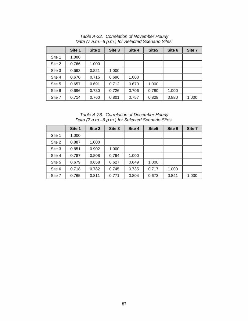
87
Table A-22. Correlation of November Hourly
Data (7 a.m.–6 p.m.) for Selected Scenario Sites.
Site 1 Site 2 Site 3 Site 4 Site5 Site 6 Site 7 Site 1 1.000
Site 2 0.766 1.000 Site 3 0.693 0.821 1.000
Site 4 0.670 0.715 0.696 1.000 Site 5 0.657 0.691 0.712 0.670 1.000
Site 6 0.696 0.730 0.726 0.706 0.780 1.000 Site 7 0.714 0.760 0.801 0.757 0.828 0.880 1.000
Table A-23. Correlation of December Hourly Data (7 a.m.–6 p.m.) for Selected Scenario Sites.
Site 1 Site 2 Site 3 Site 4 Site5 Site 6 Site 7 Site 1 1.000
Site 2 0.887 1.000 Site 3 0.851 0.902 1.000
Site 4 0.787 0.808 0.794 1.000 Site 5 0.679 0.658 0.627 0.649 1.000
Site 6 0.718 0.782 0.745 0.735 0.717 1.000 Site 7 0.765 0.811 0.771 0.804 0.673 0.841 1.000

88

89
Distribution External distribution (distributed electronically unless otherwise noted): 1 EPRI Attn: Tom Key 942 Corridor Park Blvd. Knoxville, TN 37932 3 HECO Attn: Leon Roose Mark Matsura Dora Nakafuji 820 Ward Avenue Honolulu, HI 96814 2 KIUC Attn: Mike Yamane John Cox 4463 Pahe’s Street, Suite 1 Lihue, HI 96766-2000 1 New Mexico State University Attn: Dr. Satish Ranade Klipsh School of ECE, Box 3001, Dept. 3-O Las Cruces, NM 88003 1 New Mexico State University Attn: Andrew L. Rosenthal Box 30001/Dept. 3SOL Las Cruces, NM 88003-8001 1 NRECA Cooperative Research Network Attn: Edward Torrero 301 Wilson Boulevard, SS9-204 Arlington, VA 22203-1860 1 OUSD(AT&L)/PSA/LW&M Attn: Paul C. Butler (paper) 3090 Defense Pentagon Washington, DC 20301-3090

90
8 U.S. Department of Energy Attn: Dr. Samuel F. Baldwin Gil Bindewald Tien Q. Duong Richard J. King Eric M. Lightner Philip N. Overholt Neil P. Rossmeissl Dan T. Ton 1000 Independence Avenue SW Washington, DC 20585-0121 1 U.S. Department of Energy Attn: Dr. Imre Gyuk OE-10/FORS 1000 Independence Ave. SW Washington, DC 20585-0270 1 U.S. Department of Energy Attn: William Parks MS OE-1 1000 Independence Ave. SW Washington, DC 20585-0270 1 U.S. Department of Energy Attn: Steven Lindenberg MS EE-20 1000 Independence Ave. SW Washington, DC 20585-0270 1 U.S. Department of Energy - Albuquerque Operations Office Attn: Dan Sanchez Kirtland Air Force Base Pennsylvania & H Street Albuquerque, NM 87185 1 U.S. Department of Energy, Solar Systems Integration Attn: Kevin Lynn Alvin Razon
Solar Energy Technology Program 950 L'Enfant Plaza Washington, DC 20585
1 University of Hawaii Attn: Dr. Bor Yann Liaw 1680 East West Road, Post 112A Honolulu, HI 96822

91
1 UWIG Attn: Charles Smith Utility Wind Integration Group
PO Box 2787 Reston, Virginia 20195 USA
Internal distribution (distributed electronically unless otherwise noted): 1 MS0613 Rudolph G. Jungst 2548 1 MS0614 Tom Hund 2547 1 MS0614 Peter Roth 2546 1 MS0734 Ward I. Bower 6111 1 MS1033 Christopher P. Cameron 6112 2 MS1033 Abraham Ellis 6112 (1 electronic & 1 paper) 1 MS1033 Charles Hanley 6112 1 MS1033 Joshua Stein 6112 1 MS1033 Jimmy Quiroz 6112 1 MS1108 Dan Borneo 6113 1 MS1108 Garth Corey 6113 1 MS1108 Ross Guttromson 6113 1 MS1108 Georgianne Huff 6113 1 MS1188 Stan Atcitty 6114 1 MS0899 RIM-Report Management 9532 (1 electronic)

92