KEEPIN' 'EM DOWN ON THE FARM:

MIGRATION AND STRATEGIC INVESTMENT IN CHILDREN'S SCHOOLING*

Robert Jensen

Department of Public Policy

UCLA

and

NBER

Nolan Miller

Department of Finance

University of Illinois at Urbana-Champaign

and

NBER

Abstract: In rural areas of many developing countries, intergenerational coresidence is both widespread

and an important determinant of well-being for the elderly. Most parents want at least one child to remain

at home, for example so they can work on the farm or provide care and assistance around the household.

However, children themselves may prefer to migrate to a city when they grow up, and parents cannot

directly prevent them from doing so. We present a model where parents may strategically limit

investments in some children's education so that they will not find it optimal to migrate when they reach

maturity, and will thus voluntarily choose to remain home. We test this theory using an intervention that

provided recruiting services for the business process outsourcing industry in randomly selected rural

Indian villages. Because awareness of these high-paying, high education, urban jobs was limited at

baseline, the intervention increased the attractiveness of migration for educated children. Consistent with

the model, we find that those children that parents report at baseline they want to remain home experience

declines in enrollment in response to the treatment. Though those children that parents want to migrate

have increased enrollment, and parents want more children to migrate.

JEL Codes: I12, J14, O12, O15.

Keywords: Education; Aging; Migration; Economic Development.

* Financial support from the Center for Aging and Health Research at the National Bureau of Economic

Research, the Women and Public Policy Program, the Dean's Research Fund and the William F. Milton

Fund at Harvard University is gratefully acknowledged.

1

I. INTRODUCTION

In most developing countries, children play an important role in the well-being of their

parents in old age. Children provide financial support, labor on the family farm or business,

insurance in case of illness or disability, physical care and assistance around the home, protection

and security, as well as attention and affection. These benefits are often provided directly

through parents and children living together. Over 70 percent of individuals 60 and older in the

developing world live with their children, with rates as high as 80 to 90 percent in countries such

as Bangladesh, India, Pakistan and Senegal (UN 2005).1

However, increasing urban economic opportunities as part of the process of economic

development cause many children to migrate either temporarily or permanently out of rural

areas. For many households, migration is a critical strategy for increasing wealth, with children

sending or bringing home money. However, parents cannot always rely on these transfers, and

the amount sent may be less than what the parents would prefer, or what they would get if the

child stayed on the farm and the parent, rather than the child, controlled the distribution of wealth

between them. And market-based substitutes for the other benefits of coresidence, such as care

and assistance around the home, are often imperfect or non-existent.2 In short, in rural areas of

most developing countries, intergenerational coresidence is among the most important

determinants of the well-being of the elderly, and most parents hope that at least some of their

children will live with or near them when they get older.3

Parents in general often cannot directly control whether their children migrate, and

parents and children may disagree on the decision. However, parents do control the amount of

schooling they provide their children, and may therefore be able to limit their children's potential

future benefits from migration. In this paper, we test whether some parents strategically limit

1 Similar patterns held in currently-wealthy countries in the past. In the U.S., 70 percent of the elderly

lived with their adult children in the mid- to late-19th century (Costa 1998, 1999, Ruggles 2007). 2 Knodel et al. (2007) note that while migration led to financial gains for rural elderly in Thailand,

migrant children are much less likely to provide care and other services around the home. Though Knodel

et al. (2010) note that extended households adapt to the changes brought about by migration, and that

technologies such as cell phones and faster transportation reduce the losses caused by not living together. 3 In wealthier countries, the elderly may prefer to live on their own when they can afford to. Costa (1999)

and McGarry and Schoeni (2000) show that social security reduced intergenerational coresidence in the

U.S. In contrast, Manacorda and Moretti (2006) argue that coresidence is a normal good for Italian

parents. They also present evidence that the preference for coresidence may vary across countries.

2

investments in their children's education so that they will no longer find it optimal to migrate

when they reach maturity, and thus will voluntarily choose to remain "down on the farm."

We first present a model of rural human capital investment in the face of possible urban

migration. The model predicts that when the urban returns to schooling increase, more rural

parents will be better off if their children migrate (via greater expected remittances). Parents who

are better off with their children migrating will also give them more education. Both predictions

are consistent with standard models. However, our model also yields the unique prediction that

parents who are better off if their children remain at home may respond to increases in the urban

returns by decreasing their children's schooling so that those children will choose not to migrate.

We test these predictions using an intervention that in effect increases urban economic

opportunities for households in randomly selected rural Indian villages. For three years, we paid

professional recruiters to help young men and women become aware of and get jobs in the newly

burgeoning business process outsourcing (BPO) industry (e.g., call centers, online technical

support, etc.). The BPO industry presents an ideal setting for testing our theory because jobs in

this sector are almost exclusively urban-based, require more education than traditional jobs, and

pay more than other jobs with comparable education requirements, thus raising the urban returns

to schooling (while largely leaving rural opportunities unchanged). And because the sector was

so new at the time of our study, awareness of these jobs was low in rural areas, which allows the

intervention to serve as a shock to the urban returns to schooling (while largely leaving rural

returns unchanged) and the desirability of future migration for more educated children.

Using a panel survey of rural households, we find support for the theory of strategic

investment. Those boys that parents at baseline report wanting to live at home when they are

older experience reduced school enrolment in response to the treatment. Though those that

parents want to migrate experience increased enrolment. The treatment also increased schooling

for girls, very few of whom are expected to remain at or near home due to prevailing marriage

patterns. Finally, the treatment also cause parents to want more children to migrate.

The results may help explain why education levels, particularly at the secondary level,

remain low in many developing countries, as well as why more recently, girls' schooling in many

countries has been increasing more rapidly than that of boys. The results also suggest that factors

and policies outside of the education sector, such as social security, health or nursing care, or the

functioning of land and labor markets, may affect educational attainment. Finally, they may also

3

provide an additional rationale for compulsory schooling laws, since parents may not always

invest in a way that promotes the child's best interest.

We argue that the results are consistent with parents trying to prevent some children from

migrating to take advantage of the new urban opportunities. However, we cannot definitively

identify the motives for doing so. Though intergenerational coresidence is widespread and there

is a large literature on parents' desire to have a son remain at or near home for the reasons

mentioned above, we cannot rule out that parents try to keep some children from migrating

because they believe it is in the child's best interest, rather than their own (though we present

arguments for why this is less likely to be the case). For example, parents may believe that

children overestimate the likelihood of employment in the city or underestimate the potential

costs or risks of migration. However, the same broader conclusion of strategic investment

remains: parents use education as an instrument to influence the child's migration decision when

they anticipate that they will disagree on the optimal outcome.

Others have noted the conflict arising from the fact that while parents decide and pay for

investments in their children‟s schooling, the returns accrue directly to children. For example,

Chakrabarti, Lord and Rangazas (1993) argue that since parents can't contract with their children,

uncertainty over future support can lead to inefficiently low educational investments.4 Though

we share this prediction, a key distinction is our model's prediction of declines in education for

some children in response to increases in urban returns, as opposed to just a weaker response.

Our study is also related to two other literatures. First, others have considered whether

parents act to ensure greater attention or support from children in old age. Bernheim, Shleifer

and Summers (1985) argue that parents strategically condition bequests in order to maximize

attention provided by their children. Hoddinott (1991) finds broadly similar results for Western

Kenya with respect to children's contributions of both money and time. Manacorda and Moretti

(2006) argue that Italian parents use transfers to "bribe" their children into living with them.

Additionally, many studies have considered the effects of migration on education. Most

studies focus on the potential for increased schooling, either due to greater household income

(e.g., Yang 2008) or increased returns to education. Kochar (2004) finds that rural education in

India increases in response to increases in the returns in the nearest urban labor market. She also

4 Baland and Robinson (2000) and Bommier and Dubois (2004) argue that child labor may be inefficient

if parents don't internalize, respectively, the child's reduced future earnings or disutility of labor.

4

finds that the gains are smaller for households with the most land, where children are more likely

to remain home rather than migrate. A few studies though have focused on the possibility that

migration could worsen educational outcomes. de Brauw and Giles (2008) find that increasing

possibilities of urban migration in rural China cause declines in high school enrollment. They

argue this is due to increases in the opportunity cost of schooling, via an increase in the local

wage rate (due to decreased local labor supply) or by the high wage opportunities for unskilled

workers available through migration. McKenzie and Rapoport (2010) also find that migration

may harm education because when an adult leaves, their time inputs in the production of

children's human capital is lost, and children may also have to take over household production

activities.5 Antman (2011) similarly finds a negative effect of parental migration to the U.S. on

children in Mexico, with children spending less time in school and more time working. Though

our study shares with these papers a common finding of some declines in education associated

with migration, our primary emphasis is specifically on testing the strategic investment motive

for the decline. We will also show that the mechanisms underlying these other papers are

unlikely to explain our results.

The remainder of this paper proceeds as follows. Section II discusses the model and the

testable predictions. Section III discusses the data, empirical strategy and experimental design.

Section IV shows the results and Section V concludes.

II. THE MODEL

In this section, we present a simple model of schooling investment in a two sector

economy with migration. Our goal is not to provide a complete model of such behavior, but to

demonstrate the key dynamics that generate testable predictions. We discuss the importance of

key simplifying assumptions at the end of the section. In particular, we consider a household

where the parent seeks to maximize income and there is only a single child. Doing so allows us

to clearly identify the driving force behind our results: if increasing education makes migrating

to the city marginally more attractive to the child, a parent who wishes to prevent the child from

migrating may respond to an increase in the marginal returns to education in the city by reducing

the child‟s education in order to reduce what we call the “incentive cost” of education. Having

5 They also note that if international migrants can only get unskilled jobs in the destination country

because most migration is illegal, the returns to education may be lower than without migration.

5

identified this basic force, we go on to discuss how the same idea would arise in other models,

such as with multiple children or bilateral altruism, with more complete models incorporating

these factors presented in the appendixes.

The economy has two sectors, a rural or agricultural sector and an urban sector. Each

household consists of a parent, p, and a child, c. In the rural sector, parents are endowed with a

unit of land. If the child lives on the farm, he supplies one unit of labor, i.e., the quantity of labor

is inelastic. However, their productivity does depend on their education. Let f(e) be farm output

as a function of the child‟s education, where f ' >0, f '' <0. Parents do not work (alternatively,

they are not very productive or their labor supply is inelastic). We assume for now that both land

and labor markets do not exist, so the parent is unable to sell or rent their land or hire-in labor to

work on the farm.

Children can either stay at home (H) or migrate (M) to the urban area. If the child

migrates, they send home a fraction, r, of their earnings to their parents. For now, r is taken to be

exogenous.6 There is also a cost t associated with migration, which for simplicity we assume is

paid by the child. While we treat t as a fixed parameter for the theoretical analysis, which

considers decision making within a household, t is a source of heterogeneity across households.

Thus, households with high migration costs due to factors such as distance or cultural/linguistic

differences will be less likely to migrate, while households with lower migration costs will be

more likely to migrate. A model relying on variation in the desirability of migration driven by

heterogeneity in endowments, child's ability (and thus either productivity or the returns to

schooling), the parent‟s idiosyncratic taste for coresidence, etc., would yield similar results.

Let w(e) be the wage earned by the child if he migrates to the city, where w' >0 and

w''<0. We assume that productivity is higher in farm work at low levels of education,

0 0f w , but that productivity increases more rapidly in education in the urban sector, i.e.,

' 'w e f e , so that at higher levels of education, productivity is higher in the urban sector,

w e f e , for some sufficiently large e. The cost of education is c e , an increasing and

convex function of the level of education. The results do not change if education instead has a

constant marginal cost.

6 If parents are risk averse, any uncertainty over the amount the child will remit (or the child's income if

they migrate) will reinforce the predictions of the model by lowering expected utility in old age under the

scenario where the child migrates.

6

Parents and children are assumed to be risk neutral and maximize wealth. The decisions

to be made are how much education the child should receive and whether the child should

migrate to the city.

We begin by considering the efficient outcome, i.e., the level of education and migration

choice that maximizes total household wealth. The analysis first derives the optimal level of

education for a child who remains at home and for a child who migrates, and then considers the

question of whether it is better for the family to have the child migrate or stay at home.

If the child remains at home, total household wealth is the difference between output on

the farm and the cost of schooling, f e c e . Let eHE denote the optimal education level in

this case, where ' 'HE HEf e c e . If the child migrates, total household wealth is given by

w e c e t . Let eME denote the optimal education level for children who migrate, where

' 'ME MEw e c e . Under the assumption that ' 'w e f e , i.e., the marginal product of

education is greater in the city, then schooling levels will be higher among children who migrate,

ME HEe e .

If the parent keeps the child at home, the child gets eHE years of education. If the parent

lets the child migrate, he gets eME. The former is preferred to the latter whenever:

HE HE ME ME

ME ME HE HE

f e c e w e c e t

or

w e c e f e c e t

In other words, the parent sends the child to the city whenever the maximized surplus in the city

exceeds the maximized surplus at home by at least the cost of migration.

The efficient solution will arise if the parent is able to choose the child‟s level of

education as well as whether the child migrates. However, in reality while parents are able to

exercise control over education decisions, they are less able to control migration decisions.

Further, in real contexts there is an additional incentive issue that arises due to the fact that once

a child has left the parent‟s home, the parent is no longer able to control the allocation of the

child‟s income. To the extent that parents are unable to appropriate all of the child‟s income, this

may affect their schooling and/or migration decisions. We now consider such situations.

7

If the parent cannot control whether the child migrates, we can recast the problem as a

two-stage game between parent and child. In the first stage the parent chooses the level of

education. In the second stage, the child chooses whether to migrate. We continue to assume,

however, that the child remits home a fraction r of their earnings if they migrate. The parent and

child each choose strategies to maximize their own wealth (as opposed to maximizing household

wealth, as in the efficient solution). If the child goes to the city, he remits fraction r of his wage,

leaving him net wealth 1 r w e t . Thus, in order to induce the child to remain at home, the

parent must offer him a share of household wealth of at least 1v r w e t . To simplify the

analysis and focus on the interesting cases, we assume that v > 0 for relevant levels of e and t.

That is, the child is always tempted to move to the city. If we were to relax this assumption, then

there could be a range of t and e for which v < 0. In this case, the child would choose to stay

home even if the parent gave him no resources.

In this case, the parent‟s net surplus when the child stays home is

1f e c e r w e t . Written this way, the term [(1−r)w(e)−t] is like an additional

cost of educating a child and keeping him at home given that the parent can no longer control the

migration decision. The more education the parent gives the child, the more attractive the child

finds migration, and thus the more the parent must give the child to prevent him from migrating.

If the parent wants the child to stay at home, they choose eH to maximize this function, which

occurs at ' 1 ' 'H H Hf e r w e c e . On the other hand, the parent‟s net surplus if the child

leaves is given by rw e c e , which is maximized at eM, where ' 'M Mrw e c e .

We now can state the following propositions:

Proposition 1: If r < 1, both children who stay home and those who migrate receive less

than the efficient amount of education.

Proposition 2: If r = 1, then both levels of schooling are efficient.

Proposition 3: eM > eH.

Proof: It is sufficient to show that rw’(e)>f’(e) – (1−r)w’(e). But, note that

' 'w e f e

8

' 1 ' 'rw e r w e f e

' ' 1 ' .rw e f e r w e ■

Propositions 1 to 3 establish the basic inefficiency of investments in children when

parents are unable to control whether the child migrates. We can also establish the following

results on which households‟ children migrate (as parameterized by t).

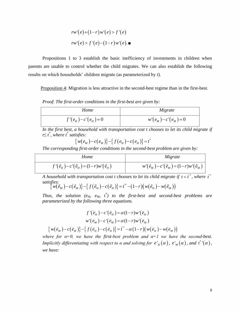
Proposition 4: Migration is less attractive in the second-best regime than in the first-best.

Proof: The first-order conditions in the first-best are given by:

Home Migrate

' ' 0H Hf e c e ' ' 0M Mw e c e

In the first best, a household with transportation cost t chooses to let its child migrate if

t≤ t*, where t

* satisfies:

*

M M H Hw e c e f e c e t

The corresponding first-order conditions in the second-best problem are given by:

Home Migrate

' ' (1 ) 'H H Hf e c e r w e ' ' (1 ) 'M M Mw e c e r w e

A household with transportation cost t chooses to let its child migrate if *t t , where *t

satisfies: * 1M M H H H Mw e c e f e c e t r w e w e

Thus, the solution (eH, eM, t*) to the first-best and second-best problems are

parameterized by the following three equations.

*

' ' (1 ) '

' ' (1 ) '

1

H H H

M M M

M M H H H M

f e c e r w e

w e c e r w e

w e c e f e c e t r w e w e

where for α=0, we have the first-best problem and α=1 we have the second-best.

Implicitly differentiating with respect to α and solving for 'He , 'Me , and * 't ,

we have:

9

*

1 '' 0

'' '' 1 ''

1 '' 0

'' '' 1 ''

' 1 0

H

H

H H H

M

M

M M M

H M

r w ee

f e c x r w e

r w ee

f e c x r w e

t r w e w e

Hence, in moving from the first-best to second-best, education levels for those who stay

home and those who migrate decrease, and the set of households for which migration is

optimal decreases. ■

Taken together, Propositions 1 to 4 establish that all children get too little education in

the second-best model. For those children who migrate to the city, the fact that parents receive

less than the full marginal product of their efforts leads the parents to underinvest in their

education. For those who stay home, parents know that the more they invest in their child‟s

education, the greater the child‟s opportunity as a migrant, and so the more the parent will have

to pay the child to induce them to stay home. Thus, in this case as well, the parent does not gain

the full marginal product of his investment in education, which leads to underinvestment.

Finally, when parents are unable to control migration decisions and fully appropriate the benefits

of children who move to the city to earn higher wages, migration becomes less attractive to

parents. They would rather receive the entire income of a less-productive child who stays at

home than only part of the income of a more-productive child in the city. However, since parents

cannot directly prevent children from migrating, the only tool they have available to them is to

reduce their schooling in order to make migrating less attractive.7

To consider the impact of an increase in returns to education in the city, we replace the

wage function w(e) with w e . Here, an increase in 0 represents an increase in the returns

to education in the city. The solution to the second-best problem, (eH, eM, t*), solves:

7 Parents may have other instruments available to either keep children at home or ensure an optimal level

of transfers from migrated children, such as threatening to withhold inheritance (in rural areas of poor

countries, this would primarily take the form of land), as in Bernheim, Shleifer and Summers (1985).

However, if the urban returns are sufficiently high or the value of land or other assets sufficiently low, the

child could still be better off forgoing inheritance in favor of migration. Further, since rural land markets

are relatively thin in many low income countries, bequests often require the child to return to the rural

area to get value from the bequests, which may make remaining in the urban area and forgoing the

bequest optimal. Finally, there many landless households, for whom bequests are generally very small.

10

*[ 1 ] ,

' 1 ' ' ,

' ' .

H H H M M

H H H

M M

f e c e r w e t r w e c e

f e r w e c e and

r w e c e

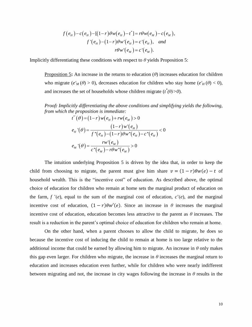
Implicitly differentiating these conditions with respect to θ yields Proposition 5:

Proposition 5: An increase in the returns to education (θ) increases education for children

who migrate (e'M (θ) > 0), decreases education for children who stay home (e'H (θ) < 0),

and increases the set of households whose children migrate (t*(θ)>0).

Proof: Implicitly differentiating the above conditions and simplifying yields the following,

from which the proposition is immediate:

*' 1 0

1 '' 0

'' 1 '' ''

'' 0

'' ''

H M

H

H

H H H

M

M

M M

t r w e rw e

r w ee

f e r w e c e

rw ee

c e r w e

The intuition underlying Proposition 5 is driven by the idea that, in order to keep the

child from choosing to migrate, the parent must give him share of

household wealth. This is the “incentive cost” of education. As described above, the optimal

choice of education for children who remain at home sets the marginal product of education on

the farm, f ‟(e), equal to the sum of the marginal cost of education, c‟(e), and the marginal

incentive cost of education, . Since an increase in θ increases the marginal

incentive cost of education, education becomes less attractive to the parent as θ increases. The

result is a reduction in the parent‟s optimal choice of education for children who remain at home.

On the other hand, when a parent chooses to allow the child to migrate, he does so

because the incentive cost of inducing the child to remain at home is too large relative to the

additional income that could be earned by allowing him to migrate. An increase in θ only makes

this gap even larger. For children who migrate, the increase in θ increases the marginal return to

education and increases education even further, while for children who were nearly indifferent

between migrating and not, the increase in city wages following the increase in θ results in the

11

parent no longer being willing to give up enough resources to keep them at home. The result is

that more children migrate after the increase in θ.8

Thus, an increase in the urban returns to education decreases schooling of children who

remain in the rural area, and increases it among children who migrate. If enough children will

remain in the rural area, the net, overall education of rural children could decrease. Additionally,

these effects will lead to greater inequality in educational attainment among rural children.

The incentive cost of education is the primary factor that leads to the prediction that

parents who wish their children to remain at home may respond to increases in the returns to

education in the city by reducing the child‟s education. This force will be present in a wide

variety of models. For example, although our simple model takes the parent as maximizing

income, similar predictions would arise in a model where the parent is altruistic if, given those

altruistic preferences, the parent wishes the child to remain at home while the child prefers to

migrate. If this is the case, then the parent will have to dedicate more of the household‟s

resources to the child to keep him from migrating than what is ideal even when the parent is

altruistic. Thus, a parent who ideally would like to split household resources evenly between

parent and child might have to divert 60 percent of household resources to the child to keep him

from migrating. An increase in the returns to education in the city would increase the child‟s

temptation to migrate, causing the parent to have to divert even more resources to the child to

prevent migration. However, if the parent can reduce the relative attractiveness of migration by

reducing the child‟s education, then the parent may respond to an increase in the urban returns by

reducing the child‟s education (see Appendix A for a treatment of this case).

The incentive cost of education can also arise in a model with multiple children. Briefly,

consider a parent with N total children who wishes to keep H of them at home and to allow M =

N – H to migrate. In order to prevent the H children from migrating, the parent will have to

ensure that they are as well off at home as they would be if they migrated. This constraint gives

8 Although the parameterization of the returns to schooling as w(e) allows us to easily compute the

effects of an increase in θ on education levels and t*, the result holds more generally. In particular, the

same qualitative conclusions hold if we instead consider an upward shift in w'(e). To see this, note that eH

is defined by f '(eH) – (1−r)w'(eH) = c'(eH), which only depends on eH. An upward shift in w' (e) decreases

the left-hand-side, which decreases the optimal choice of eH and lowers the parent‟s maximal surplus

from keeping the child at home. Similarly, eM is defined by rw'(eM) = c'(eM), and an upward shift in w' (e)

increases the left-hand side, which increases the optimal choice of eM and increases the parent‟s optimal

surplus from letting the child migrate. t* then necessarily increases because the cut-off level of t is where

* 1M M H H Ht r w e c e f e c e r w e

12

rise to the incentive cost of migration. Beginning with the case where the parent has optimally

chosen education levels for the children and which should migrate, an increase in the returns to

education will increase the temptation to migrate of those who stay at home. Once again, if the

parent wishes to prevent the children from migrating, they will have to be given more income.

However, the parent can also reduce the temptation to migrate by reducing the children‟s

education. We show in Appendix B that reducing education in response to an increase in the

returns to education may be optimal for the parent.9

We have abstracted thus far from the portfolio decision allocating education and

migration across multiple children. In such a setting, for any particular child the education and

migration effects of increasing urban returns are likely to be influenced by what is optimal across

the collection of siblings. Thus for example, in response to an increase in the urban returns,

credit constrained parents may find it optimal to focus their limited resources on fewer children,

with some gaining at the expense of others. Parents with two children may decide that rather than

providing both with an intermediate amount of schooling, they should instead now provide one

with a high level of education (and/or higher quality or more expensive private schooling) so

they can get a BPO job, requiring a schooling reduction for the other (see Appendix C), cutting

back for the other. Whether this is optimal from the parent's perspective will depend on the shape

of both the urban and rural returns functions and the schooling cost function. Such cross-sibling

effects could also occur through a reallocation of time in household production activities (the

child expected to remain at home takes on more so that the child expected to migrate can focus

more on schooling, leaving the former with less time for school). We will not analyze this

portfolio decision, since our focus is on testing the down on the farm hypothesis. However, the

multiple child case does raise an important issue for the empirical analysis, since both our model

and credit or household production constraints under multiple children predict gains for children

expected to migrate alongside losses for children expected to stay at home. We address this

further in Section III.F.

As noted in the introduction, there are several reasons other than income why parents

may not want children to migrate. For example, children may provide services for which market

9 When there are multiple children at home, one complication is that reducing the education for any one

child affects the marginal productivity of the other children. Under relatively weak assumptions, it can be

shown (Appendix B) that it remains optimal for the parent to reduce education for all children who

remain home following an increase in the returns to education in the city.

13

substitutes are imperfect or effectively non-existent, such as physical care, attention, affection or

protection from crime or violence. Alternatively, parents may place greater value on maintaining

traditional ties to ancestral land than children do, worry more about the "corrupting influences"

of cities or place less value on their social amenities. In any of these cases, children are more

likely to migrate to the city than parents would prefer. If parents do not directly control the

migration decision but do control the education decision, and if lower levels of education reduce

the child's reward from moving to the city, similar results would arise under these alternative

motives. Distinguishing among motives will not be possible with our data. Our primary interest

is whether parents engage in strategic behavior to influence their child's migration decision, so

our analysis will focus simply on how education responds based on whether parents want a given

child to migrate, regardless of the underlying reason.

We made several other assumptions in setting up the model. First, we assumed there were

no land markets. If the parent could simply sell their land for the discounted stream of future

output, they would not need to have a child stay to work the land. Alternatively, they could lease

the land to someone else to farm (either for rent or as part of a share cropping arrangement).

However, land markets are often imperfect in many rural areas, and there are not many

transactions in practice, so that this assumption remains a crude but fair approximation for at

least some households. There are many reasons these markets are limited. In rental markets, for

example, there are problems in contract enforcement, and differing incentives between landlord

and renter with respect to the short vs. long term health and productivity of the land (i.e., some

agricultural techniques result in higher short-term yields at the expense of longer-term yields).

With respect to land sales, one limitation is imperfect titling and tenure security. In

addition, it would typically be difficult to store wealth from a sale, since there is little access to

banks or other formal savings instruments, particular in rural areas, and less formal means of

wealth accumulation may not be sufficiently safe, or protected from the demands of relatives.

Further, individuals may attach a psychic value to land that has been in their family for

generations (which the market will not compensate), and want their sons to keep it in the family.

Further, in some areas of the developing world, households may have only usufructury rights to

land, meaning they have rights to the exclusive use of a given parcel of land, and can bequeath

those rights to their children, but they cannot sell their land or rent it to others. Under such

arrangements, if the land is unused, village authorities may reassign it to other households,

14

without compensation. The inability to sell the land means that the only way for the parent to

extract the future value of that land is if their child remains at home on the farm (or, if they can

hire in labor, as discussed below). Although in practice land markets in rural areas are often not

very robust for these reasons, we of course would not argue that there is no land market at all.

However, there are strong factors that favor retaining owned land, which creates an additional

wedge that the higher expected contributions of migrating children must overcome. And it is also

worth noting that even with perfect land markets, our results would still hold if parents don't

want children to migrate primarily because there are no market substitutes for the other benefits

of coresidence or because of an aversion to children living in the city, since then what matters to

the parent is just whether the child physically stays or migrates, not whether the parent can

maintain income by selling their land.

We also assumed that there were no labor markets. With perfect labor markets where

parents can hire-in workers to replace migrating children, there would be again be less financial

reason to prefer a child remain at home. However, labor markets are often imperfect as well.

Hired labor may not yield as a high a return to the parent, such as due to greater monitoring and

enforcement costs. Foster and Rosenzweig (2011) estimate that using hired-in labor rather than

family labor doubles the shadow price of labor, such as due to higher supervisory costs.

Additionally, a temporary worker who may change from season to season will also not have the

farm-specific human capital or "specific knowledge" that a child growing up and working on that

farm over many years will have. Rosenzweig and Wolpin (1985) use specific knowledge to

jointly explain the predominance of extended families, the predominant use of family labor on

farms, and the relative scarcity of land transactions in rural India. Finally, there may also be an

unwillingness to hire-in labor that may expose women in the household to men outside of the

family (restrictions such as purdah are practiced by about 10 percent of households in our study

area). Again, we would not argue that agricultural labor markets don't exist, but rather there are

strong factors that favor the use of family labor, as has been documented by others, and which is

frequently observed in practice. And again, even with perfect labor markets, children who

migrate are unable to provide the non-financial benefits of coresidence for which there are no

market substitutes, so parents may still prefer a child remain at home.

15

III. DATA AND EMPIRICAL STRATEGY

III. A. Study Area and Survey Information

We focus on rural areas outside of Delhi, one of the major centers of the Indian BPO

sector. Because we wanted to test our model where awareness of BPO jobs was low, we used

experienced BPO recruiters from Delhi to define the areas outside of the city where recruiters

were not visiting, due solely to distance or population size, i.e., the time and cost per potential

recruit was high enough that it was not worthwhile to search for potential recruits there.10

This

primarily meant focusing on areas approximately 50 to 150km outside of the city, in the states of

Haryana, Punjab, Rajasthan and Uttar Pradesh. Within this area, we drew 160 villages at random

from a list of all villages. In each village, we worked with local officials to draw up a list of all

households, then randomly selected 20 households per village.

We conducted a baseline survey from September to October of 2003, using students at

the Management Development Institute, a nearby business school. The survey consisted of a

household questionnaire, an adult questionnaire and a survey of village characteristics conducted

with knowledgeable local officials. We also gathered information on all household members, or

children of members, who were temporarily or permanently living away from home. Therefore,

we know for example about the enrollment status of children who have migrated.

A follow-up survey with the same households was conducted from September to October

of 2006. We also tracked, and where possible interviewed, all individuals who left home between

rounds, such as for work or marriage. Means and standard deviations of key variables are

provided in Table I.

III. B. Testing Predictions of the Model

The key testable predictions of the model from Proposition 5 are that for rural areas, an

increase in the urban returns to schooling should lead to:

Prediction 1: An increase in schooling for children whose parents want them to migrate;

Prediction 2: A decrease in schooling for children whose parents do not want them to migrate;

10

At this range, due to poor road quality and high congestion around Delhi, a Delhi-based recruiter might

need to spend a whole day, and considerable travel expenses, just to reach one village. And any given

village may have only a few individuals with enough education for a BPO job. Since recruiters typically

earn a fee per recruit they find, it is far more profitable to focus on Delhi than on outlying rural areas.

16

Prediction 3: An increase in the number of children parents want to migrate.

The two biggest challenges in testing these predictions are, 1) classifying children based

on their parents' preferences towards migration, and 2) a source of exogenous variation in the

urban returns to schooling. We discuss each of these in detail below.

III. C. Classifying Children by Parent's Migration Preferences

A number of factors may affect whether a parent wants a given child to migrate,

including the amount of land owned, the quality of labor and land markets, beliefs about the

child's altruism or their ability in both rural and urban occupations, expectations about health and

life expectancy, preferences over factors like keeping land in one's family or the corrupting

influence of city life, etc. Our survey cannot provide a complete accounting of all the

determinants of migration intentions. Instead, we use a direct elicitation of intentions or

preferences. Respondents were asked, for each of their living children, "When you are much

older and your child is an adult, do you want or hope [child] will live: 1. in this dwelling or in

another dwelling on this land or compound; 2. in a separate household or dwelling in this village;

3. in a different village, nearby; 4. in a different village, far away; 5. in a city in India; 6. in a

country other than India."11

We take the response to this question as a summary, reduced-form

measure of parents' migration preferences.

There are of course concerns in using self-reported preferences or expectations.12

However, an increasing number of studies have shown that such measures can be good

predictors of actual future outcomes, as well useful indicators of underlying beliefs that can be

11

Since some migration may be temporary, additional questions were asked as follow ups. For the first

four responses, a follow-up asked: "Do you hope [child] will go live and work in a city at any time in the

future for at least 6 months, even if they return after that?" For all responses other than 1 or 2, a follow-up

was (also) asked: "Do you hope [child] will eventually return and live with you in the same dwelling or in

another dwelling on this land or compound, or in a separate household or dwelling in the same village?" 12

Classifications based on more objective variables have limitations. For example, in some areas, by

custom only the oldest son inherits land or is expected to remain home with his parents. However, this

norm is not universal, so birth order is not a useful classifying measure. Another alternative is land

holdings, since those with little or land would not expect their children to stay to work their land.

However land is also wealth, which might affect education. And parents without land might still want

their children to remain nearby to provide care or assistance or to run a family non-farm business.

17

used for testing theories in the way we wish to here.13

In addition, any concerns about whether

subjective measures accurately capture the underlying factor of interest should cause the variable

to contain less true signal about migration preferences and thereby weaken our test of the model,

which will rely on differences in parental migration intentions across children. However, an

important concern is whether this measure simply proxies for other factors that influence

schooling. However, the key distinguishing prediction of our model is that an increase in the

urban returns will have a negative impact on schooling for children that parents want to stay at

home; though many factors may cause parents to not increase their children's schooling in

response to these new opportunities, it is difficult to think of factors that would cause a decrease,

unless it is directly tied to not wanting children to take advantage of the new opportunities, as in

our model. Thus for example, parents may understandably not give their less intelligent children

more education following our intervention because they don't think those children can get BPO

jobs, but it is unclear why they would give them less education in response to the treatment,

other than to keep them from trying to migrate for the job. Though below, we will consider the

possible effects of credit constraints, changes in local labor market conditions or changes in

household time allocation.

We also note that if parents simply report what they believe is fait accompli, i.e., the child

has already made it clear whether they will migrate, rather than what the parents themselves

prefer, this should not generate our results; there is no reason to expect that parents who have

resigned themselves to the child having decided to stay home would respond to the increased

urban opportunities by giving them less schooling.

Table II shows baseline responses to the questions about migration preferences for

children aged 6 to 18 at baseline. Parental preferences for boys show considerable variation.

Parents want about 44 percent of boys to live with them in the same physical dwelling or

compound when they are older, and want another 24 percent to live in the same village. The

desire to have a son stay nearby is even stronger than this implies, since many couples have more

than one son; over 80 percent of parents want at least one of their sons to live with them when

13

For example, Finkelstein and McGarry (2006) find that subjective beliefs of the likelihood of entering a

nursing home predict the decision to purchase long-term care insurance and actual future nursing home

entry. They also use this variable to distinguish risk aversion from adverse selection. Similarly,

Jayachandran and Kuziemko (2010) test a model of breastfeeding duration based on how close a

respondent is to self-reported "ideal family size." Manski (2004), Hurd (2009) and Delvande, Giné and

McKenzie (2010) provide discussions of measures of subjective expectations and their limitations.

18

they are older. Parents want 15 percent of boys to migrate to a city. However, there is very little

desired rural-to-rural migration (either to nearby or distant villages) or migration outside of

India. Finally, about 5 percent of responses were "don't know," "doesn't matter," "whatever the

child wants," or "up to god."

Preferences for girls differ notably. Parents want very few girls to live in the same

dwelling or village as them, instead wanting about 48 percent to live in another rural area (either

nearby or further away). These preferences are consistent with the common practice of patrilocal

exogamy, where marriages take place across rather than within villages, with girls leaving their

birth household to join their husband's family. Parents want 23 percent of girls to migrate to a

city, but want very few to leave India. There were also more instances in which parents reported

don't know/whatever the child wants/up to god (16 percent). Because parents report wanting so

few girls to remain home or in the same village, there is little need for strategic underinvestment

to keep them from leaving. Thus, we will not be able to test Prediction 3 for girls.

We note that because these preferences predict that boys may experience the strategic

reductions in schooling but girls will not, our model shares a common prediction with Munshi

and Rosenzweig (2006). They find that increases in the returns to English language education in

Bombay driven by the financial sector and other white collar industries caused increased

enrollment in English language schools for girls but not boys. They attribute the difference to

caste-based job networks, which women were not a part of and that appear to limit men's

occupational mobility. Our studies share the prediction of how a cultural practice or institution

can cause a seemingly gender neutral increase in the returns to schooling to have heterogeneous

effects on children by sex, and in particular predicting that the gains may be greater for girls.

For testing our predictions for boys, we will use the fifth response, wanting the child to

live in a city, as our indicator of parents wanting them to migrate, and the first two responses,

wanting the child to live in the same dwelling or compound, or in the same village, as not

wanting the child to migrate. In terms of the latter, many of the roles sons (and/or their wives)

play in the lives of their elderly parents, such as working on their land or providing care around

the home can best be provided, or are most likely to be provided, when they coreside.14

However, much of the same can also be accomplished without living in the same physical

14

A son's wife may remain behind even if the son migrates, and provide labor, care and support to her in-

laws. Though this certainly happens, there is in total less help provided when the son migrates, and

additionally, many men who migrate will bring their wives and children with them.

19

dwelling, provided children are nearby, such as in the same village, as noted for example by

Bian, Logan and Bian (1998) for China.15

And, for some motives, such as simply not wanting a

child to live in a city because of perceived dangers, the parent will be indifferent between living

together or having the child in the same village. The key issue for our analysis is that when there

are new opportunities available in the city, some parents will want their children to take

advantage of those opportunities, and some will want their children not to, and in particular will

want them to remain nearby. The first and second responses seem the most appropriate way to

capture this latter category. We do not include the other responses (wanting the child to live in

another village, nearby or far away, or to live outside of India) in our analysis.16

III. D. Variation in the Returns to Schooling: The Recruiting Experiment

Testing the model also requires variation in the urban returns to schooling. We make use

of an experimental intervention that in effect assigned greater urban opportunities to randomly

selected rural villages by using recruiters for the BPO industry. The BPO industry covers a range

of activities such as call centers, data entry and management, claims processing, secretarial

services, voice-to-text transcription and online technical support. The sector has grown rapidly

over the past decade in India due to technological changes in telecommunications and

networking infrastructure, such as the deployment of fiber optic cable networks, and regulatory

changes, such as allowing foreign investment in the telecommunications sector. This growth

created a sharp and sudden increase in the demand for educated workers. To help BPO firms

meet this demand, a specialized recruiting sector grew, which included small and medium sized

firms that would seek out and screen potential employees, either freelance or under contract

(some larger BPO firms also developed their own in-house recruiting divisions).

15

Living in a city also does not preclude visiting parents, providing seasonal labor or occasional care

around the home. However, it is likely that the amount of such activity will be greater on average when

the child lives nearby. The same holds for responses 3 and 4, wanting the child to live in a nearby or

distant village. Though if parents' primary concern about migration relates simply to not wanting their

child to live in a city, we might expect parents to reduce education for this group as well. 16

For our tests, wanting the child to live outside of India should not be included as wanting the child to

migrate. The experiment increased the returns to schooling in urban India. If a parent wanted their child to

live and work outside of India, we would not expect them to alter their education investments based on

these new opportunities (unless it changed whether parents want them to stay in India, and the amount of

education for the desired overseas work differs from what is required for BPO jobs).

20

The BPO sector is well-suited for testing our predictions. First, BPO jobs require at least

a high school degree, and offer much higher salaries on average than other jobs with similar

educational requirements. Entry-level salaries typically ranged from 5,000−10,000 Rupees

($U.S. 110−220) per month in 2003, which was about twice the average salary for workers with

a high school degree working in other sectors. Therefore, the growth of the BPO sector

represents an increase in the returns to schooling. Oster and Millett (2011) similarly treat the

BPO sector as a shock to the returns to schooling, and Shastry (2012) uses the information

technology sector in India more broadly in a similar way.

Second, at the time of our study, BPO jobs were located almost exclusively in urban

areas, thus there was specifically an increase in urban returns to schooling, as in our model,

leaving the rural returns largely unchanged (we test this in more detail below). Third, because the

sector was so new at the time we began our study, there was very limited awareness of the BPO

sector itself or how to get a BPO job, particularly in rural areas, which we will focus on. In our

2003 baseline survey, discussed below, less than five percent of respondents reported they had

ever heard of call center jobs.17

And no household had a member, including those living

temporarily or permanently away from home, working in this sector. This allows us to increase

the urban returns to schooling from the perspective of rural parents by increasing awareness of

these jobs and making it easier for qualified individuals to get them, as detailed below.

We view our intervention as having primarily speeded up the timing at which households

learned about the BPO sector and received contact from recruiters, since at baseline, recruiters

told us that they expected recruiting activities to eventually expand further out over time (as they

have since done), as well as for information to spread via other channels such as the popular

media or word-of-mouth.

Finally, the high education requirements of BPO jobs (typically a minimum of 10 or 12

years of schooling) will help us treat our intervention as increasing the future urban returns to

schooling for currently young children, while largely leaving the employment opportunities for

older adults in their household unchanged. One concern in analyzing the effects of labor market

conditions on contemporaneous changes in schooling is that the labor market affects both

children in the future as well as adults in the current period. It can therefore be difficult to

17

Oster and Millett (2011) find that perceptions of the higher returns to schooling created by the presence

of a call center in a town does not spread more than a few kilometers from the actual call center.

21

determine how much of any associated change in education is driven by the anticipated future

benefits of schooling, as opposed to changes in their parents' or older siblings' current

employment or earnings (and thus changes in household income, time allocation or the

bargaining power of one parent relative to the other). Not only are few adults with school aged

children in our sample qualified for a BPO job, but we can exclude any direct effects of getting a

BPO job on children's schooling by restricting the sample to households where no member could

get a BPO job because they have too little education. We discuss this in more detail below.

For our intervention, we hired eight experienced BPO recruiters working in Delhi. Each

of the recruiters was randomly assigned to one of 80 randomly selected treatment villages (i.e.,

random assignment was two-sided).18

Between December 2003 and February 2004, recruiters

visited the treatment villages. After first making contacts and introductions, the recruiters would

return a few weeks later and conduct information and recruiting sessions, open to all members of

the community.19

The sessions followed a fixed format, including: an overview of the BPO sector and the

types of jobs and level of compensation available; information on the names of employers

currently or frequently looking for workers; strategies for how to apply for jobs (creating and

submitting resumes, lists of websites and phone numbers); interview skills lessons and tips;

mock interviews; assessment of English language skills; and a question and answer session. The

recruiters also emphasized that the jobs were very competitive, and that employment was not

guaranteed. The sessions were well-attended, and drew a great deal of interest.

The recruiters provided "booster shots" one and two years after the initial treatment,

visiting the same villages and conducting the same sessions. Recruiters also left their contact

information for free follow-up, additional information or assistance. The recruiters were

contracted to provide support for anyone from the designated villages. Thus, the intervention

consisted of three in-depth sessions plus three years of continuous, free placement support.

18

We did not stratify the treatment in any way, so there is some imbalance across districts and states.

However, as noted in Tables I and II, there are few significant baseline differences in covariates between

the treatment and control groups. Further, the results are robust to using district or state fixed effects. 19

In a second set of treatment villages, we provided recruiting services for women only. Jensen (2012)

uses these villages to test whether labor market opportunities for women affect human capital, marriage

and fertility. Since parents want few girls to stay home, and since the women-only intervention did not

directly alter the opportunities for boys, we do not use these villages for the present study.

22

The last three columns of Tables I and II report summary statistics separately by

treatment status, as well as tests of treatment-control covariate balance at baseline. The variables

overall appear balanced between the control and treatment groups. Formal tests suggest that

randomization was successful: the p-value for the F–test that baseline characteristics jointly

predict treatment is 0.63 and variable-by-variable individual t-tests in the final column cannot

reject equality of means for the treatment and control groups for almost all variables.

III.E. Empirical Specification

Our test of Predictions 1 and 2 (gains in enrolment for children that parents want to

migrate and declines for those they want to stay home) consists of regressing Round 2 school

enrolment for children 6−18 on an indicator for residing in a treatment village, separately for

subsamples based on baseline parental preferences towards the child's migration: 20

reatment

where Treatment equals one if child i lives in a village that was exposed to the recruiting

intervention. Since Table II showed that parents want few girls to stay either home or nearby, we

simply present the overall effect of the treatment for the full sample of girls.

Though randomization should result in treatment-control covariate balance in

expectation, in any particular sample there can be small differences. Therefore, we also present

results adding baseline controls, Z, that are predictors of enrolment (parent's education, log of

food expenditure per capita, family size and child age):

reatment

Finally, we also show a third specification using changes in enrolment between Rounds 1 and 2

as the dependent variable:

reatment

Though the experiment and the survey were designed to explore differential investments

based on migration preferences, we did not explicitly stratify our experiment by these intentions,

since randomization was only feasible at the village level (due to costs and possible spillovers of

20

We use baseline values to avoid stratifying by an endogenous variable. Since the treatment may cause

more parents to want their children to migrate, this likely biases us against finding the effect we predict.

23

information about these jobs to others). However, the bottom panels of Table I show that

baseline variables are still balanced within these subsamples.21

For testing Prediction 2, we use the same specifications, but with the parent's migration

preferences for each child as the dependent variable. All regressions are estimated using linear

probability models, but the results are robust to alternative limited dependent variable

specifications. Standard errors are clustered at the village level.

III.F. Distinguishing Down on the Farm Effects from Credit Constraints

As noted above, credit constraints or household production in the presence of multiple

children could yield similar predictions to the down on the farm model. Without ruling out that

such effects may cause reductions in schooling for some boys in our treatment villages, we can

test our model in a setting where such are unlikely to explain our results. For example, if we see

schooling declines for boys expected to remain home in families with just one child, it cannot be

because parents are instead investing more in another child. However, single child families are

extremely rare in our sample. As an alternative, we can consider households where there is only

one school-eligible child; for example, they are the last born child and as of Round 1 all of their

earlier born siblings are past schooling age or have permanently dropped out of school.22

In such

cases credit constraints may cause parents to not provide more schooling to the child in response

to the treatment, but they should not cause a reduction, since there is no other child to invest in.

And even if parents always intended for these children to get less education than their siblings,

there is no reason to decrease their education in response to an increase in the urban returns. If

anything, having older siblings who work (either away from home or at home) rather than attend

school should reduce credit constraints or household production labor needs.

IV. RESULTS

IV. A. Tests of the Predictions

We begin by first discussing the net effects of the treatment, before turning to the test of

our hypothesis of interest. The results are presented in Table III. The first two sets of columns

21

A second concern with ex-post stratifications in randomized trials is that splitting the data in enough

ways will always eventually yield a statistically significant relationship for some subgroup. However, that

is less of a concern here, since this analysis was an explicit part of the study design. 22

Even children who report having permanently left school could in principle return to school. However,

in our sample, we only observe four cases where such a child at baseline is enrolled in Round 2.

24

show results for the full sample of boys and girls. For girls, the treatment increased the likelihood

of enrollment by about 5-6 percentage points. The coefficient is robust across the three

specifications, and statistically significant at the 1 percent level or better in all cases. The effects

are large, representing about 7−8 percent gains relative to the control group.

By contrast, the treatment had little to no net effect on education for boys. The

coefficients across all three specifications are negative, but they are small and not statistically

significant. Again, on its own, the finding of no effect for boys is consistent with many possible

explanations beyond the offsetting effects predicted by our model; for example, there may have

already been high returns for boys even without the BPO sector.23

The last two sets of columns in Table IIII split boys based on parents' baseline migration

desires, focusing first on the full sample of such boys, rather than just those who are the last

school-eligible child.24

For the group of boys that parents want to stay at or near home, the

treatment had a negative effect on enrolment. Across the three specifications, the treatment

reduced enrolment by about 4-5 percentage points, with results statistically significant at the 5

percent level or better. This result indicates that there is a clear set of youths who lose out when

the urban returns increase, either due to our strategic investment motive or another factor such as

credit constraints.

By contrast, for the group of boys that parents want to migrate, the treatment had a

positive impact on schooling. School enrolment increased by about 6 percentage points, though

the effects are only significant at the 10 percent level (perhaps in part due to the smaller sample

sizes, since parents want fewer boys to migrate). Though consistent with more standard models

of investment in schooling, this result, as well as the schooling gains for girls, is of interest in its

own right because it suggests that for some children, poverty and credit constraints or supply-

side limitations may not be as important as demand-side constraints in limiting investment, i.e.,

parents may be providing little education to some children not because they can't afford to or

because schools are too far away, but because they don't find it optimal to, due to low expected

returns. Our experiment did not change credit constraints, wealth, school quality, distance to

23

Oster and Millett (2011) find that call centers lead to enrollment gains for boys and girls in India.

However, they examine the effect of the local presence of a call center; with call centers nearby, boys

could get a BPO job without migrating, reducing the need to strategically reduce their education. We

focus on more remote rural areas where there were no call centers, thus requiring migration. 24

Because of some non-responses, the sample sizes do not add up to the total for the full sample of boys.

25

schools, etc. The anticipated higher return to schooling was sufficient, for some children, to

induce greater schooling, as in Foster and Rosenzweig (1996), Heath and Mobarak (2011),

Munshi and Rosenzweig (2006), Jensen (2010, 2012) and Abramitzky and Lavy (2011).

Table IV shows the results for the sample of last remaining children, which enables us to

test our down on the farm hypothesis more cleanly by effectively eliminating cross-sibling

effects (i.e., they cannot be reducing one child's education in order to give another child more

education, since there are no other children in the household to give schooling to).25

This

restriction also reduces our sample size considerably. The results are less precisely estimated

than before, but we again see the same patterns as for the full sample of children. For the full

sample of girls and boys, the point estimates of the effects of the treatment are still positive and

negative respectively, but in neither case are they statistically significant. For boys expected to

migrate, the effect of the treatment is positive in all specifications, and moderately sized, but no

longer statistically significant, perhaps in part due to the sample size being reduced to just 119.

With regards to the strategic investment motive however, education again declines for those boys

that parents want to remain at home. The magnitude is in fact is slightly larger than for the full

sample of boys,26

and statistically significant (though for the specification with no additional

controls, the effect is only significant at the 10 percent level). Thus, we find evidence supporting

our model, in a setting where the results cannot be due to credit constraints. And as noted above,

while there may be a concern that wanting a child to stay home is proxying for some other

omitted child or household attribute that causes parents to give those children less schooling on

average, or that may make them not want to increase their child's schooling in response to the

new opportunities (e.g., the feel the child is not intelligent enough to get one of the jobs), there is

no obvious such factor that would cause households to respond to an increase in returns by

decreasing schooling, unless it has to do with wanting to prevent that child from migrating in

response to the new opportunities. We discuss some alternatives more fully below.

25

Though we can't rule out that some parents reduce their children's education to finance the education of

children outside of the household (e.g, nieces or nephews). However, the treatment was not associated

with an increase in transfers made, including payments made on behalf of people outside the household. 26

We might expect bigger effects for such last remaining children. If parents want an older child to

remain home but they migrate anyway, there are other children left to try to keep home. If the parent

wants the last child to remain home but they leave, there are no more options. Therefore, parents should

employ even greater strategic reductions in schooling for such children.

26

Finally, we can test the prediction that parents should want more children to migrate in

response to an increase in the urban returns to schooling. Table V shows that in response to the

treatment, parents do indeed want more children to migrate. For boys, there is a 7 percentage

point increase, which is very large relative to a baseline of 15 percent. For girls, there is a 6

percentage point increase, from a baseline of 23 percent. The new set of high paying urban jobs

clearly changes the migration vs. home calculus from the perspective of parents.

IV.B. Alternative Explanations for Declines in Schooling

As noted, the key prediction that differentiates our model from more standard models of

human capital investment or migration is that for the identifiable subgroup of children that

parents want to stay at home, the increase in urban returns leads to a decrease in schooling, as

opposed to just no response at all. We argue this is due to parents responding to the increased

likelihood their children will want to migrate by making migration a less attractive option for

them. However, a few alternative mechanisms could also generate a decline in schooling for

some children, even alongside gains for others, in the face of increased urban employment

opportunities or returns to schooling.

First, even though the BPO sector was specifically chosen for the experiment because it

targeted the employment opportunities of younger adults (or current children in the future) while

leaving opportunities for current parents largely unchanged (since few have enough education,

speak English or have computer experience), it is still possible that a few parents did get jobs. If

so, the education of children 6-18 in our regression samples could have been affected through

other channels. For example, the gains for some children could have come through greater

household income. Alternatively, declines for some children could have come through children

taking over the household production activities of parents who migrate for a BPO job, or the lost

parental time input into the child's human capital (as suggested by McKenzie and Rapoport

27

2010).27

Similar effects could be arise through BPO employment of older siblings or other adults

in the household.28

We certainly cannot completely rule out that such effects take place in our treatment

villages, and in fact we believe it is likely some such changes do occur. Instead, we would like to

test our model in a setting where these effects are unlikely to apply. Building on Jensen (2012),

we focus on the subset of households where no member could get a BPO job because they all

have too little education. As noted above, BPO jobs typically require a minimum of 10 years of

schooling. The labor market opportunities for individuals with less education were unchanged by

our experiment (unless the migration of some individuals for BPO jobs opens up more jobs

locally or increases local wages, as we explore below). It is important to keep in mind for this

analysis that we have information on all household members, whether living home or away from

home, as well as all children of household members, whether they have temporarily or

permanently left home. Therefore, we can also exclude households where older siblings of the

children in our sample may have gotten a BPO job and are no longer at home. We note that this

restriction does not change our sample dramatically, since education levels are quite low in this

rural sample (over 75 percent of households with children aged 6 to 18 in our sample do not have

any members with 10 or more years of schooling).29

The top panel of Table VI shows that the same results continue to hold for this

subsample. The treatment was again associated with declines for boys expected to stay home; the

results are similar in magnitude to those in Table III, and remain significant at the 5 percent level

or better in all three specifications. For boys expected to migrate, the results are still positive, but

slightly smaller in magnitude than in Table III, and now only 1 of the three is significant at the

10 percent level). For girls, the results are very similar to the full sample, and remain significant

at the 5 percent level or better. Again, these results do not rule out that some children's schooling

27

Employment of adults could lead to other changes affecting child's schooling, such as greater income.

However, any such effects would likely increase schooling, not decrease it. One possibility however is

that the increased earnings of one adult may increase their bargaining power relative to their spouse, and

that adult may prefer to give their child less education than their spouse does. Though we find this

possibility unlikely, excluding education-qualified households as we do next would rule out such effects. 28

In fact, we can already to an extent largely rule out effects coming through parental employment, since

no adult with a child aged 6-18 in our sample had a BPO job in Round 2. 29

Though we did not stratify our intervention by whether households had qualified members, we find that

treatment-control balance still holds for almost all variables at baseline (results available upon request).

28

in treatment villages was affected by a parent, older sibling or other household adult getting a

BPO job; but such effects are unlikely to explain the results for this subsample of households.

A second mechanism that could lead to schooling reductions for some children is that in

places where many young adults get BPO jobs, the reduced supply of labor might increase the

local wage rate and increase the opportunity cost of schooling, as suggested by de Brauw and

Giles (2008). Though there is no test to completely rule this out, we believe it is unlikely to

explain our results. The number of people induced to leave due to the treatment in any given

village is small relative to the size of the local labor force (about 3 people per year on average,

relative to the average village size of over 1,200), so any wage effects are likely to be very small.

As a more direct test, if we regress the average wage of workers on an indicator for being in a

treatment village the coefficient is very small, negative, and not statistically significant (results

available from authors upon request).30

IV.C. Motives for Strategic Underinvestment Behavior

Our model was motivated by the idea that parents strategically underinvest in their

children's education in order to keep them from migrating, and that such behavior is motivated

by parents maximizing their own well-being. While our results suggest that the reduction in

education is designed to reduce the likelihood that the child migrates (since there is no other

reason that parents would give their children less education in response to an increase in the

urban returns), our data do not allow us to rule out that parents engage in such behavior for the

benefit of the child. Parents may for example believe that the child will make a decision to

migrate that is not in their own personal best interest, such as if they believe the child is myopic

or overestimates wages or the likelihood of employment in the city or underestimates the costs or

risks of living there.

Any such concerns would have to be child specific, since most parents want some boys to

migrate and others to stay home. If parents opposed migration because of a general view that the

city is a bad place to live due to corrupting influences of cities or high crime rates, etc., then we

would not expect much variation among boys in the same household. Though it is of course

30

It is possible that for children expected to remain in the village, the future migration of other children

will decrease the future expected local returns to schooling, providing less reason to stay in school.

However, this too seems unlikely. Since it is mostly higher skilled or educated workers who will migrate

for BPO opportunities, the local returns to education might actually increase.

29

possible that a parent thinks it is less of a problem for one of their sons to move to the city than

another because they are less vulnerable to these problems (less likely to be tempted by vices,

more "street smart" and less likely to be victimized, etc.).

It also seems that since the decision to migrate is reversible, there would be little reason

to "protect" the child from themselves in this way. A child who migrates to the city and fails to

get a job could always return home. There may be a slight deterioration in farm-specific capital,

the parent may lose their farm if they can't hire in labor while the son is gone, or there may be

permanent harm associated with even temporary migration (e.g., drug or crime problems). But it

seems that other than the most extreme cases, the costs of a child migrating and then returning if

they fail would be small, especially relative to the potential lost income from instead reducing

their schooling to make sure they don't migrate.

Given the significant and well-documented roles children have long traditionally played

in the lives of the rural elderly, plus the lack of alternative sources of support and other

assistance in rural areas, and given that we can rule out general explanations such as dislike of

cities that applies to all children and that there is little reason to protect a myopic child since the

migration decision is reversible if the child migrates and fails, it seems likely that parents own

desire to have children around in old age plays some role towards explaining our results.

However, we can certainly not rule out that parents consider their actions to be in the child's best

interest (rather than, or in addition to, their own). The unifying interpretation under our model

and this alternative would be that parents anticipate a discrepancy between what they believe the

child will want to do, and what they themselves want the child to do--whether for the best

interest of the parent, the child or both. In both cases, reducing education is an attempt by the

parent to influence the child's decision (by changing the potential gains from migration) and

make it more likely they will do what the parent wants, when parents otherwise lack direct

control over that decision.

V. DISCUSSION AND CONCLUSION

Using a randomized BPO recruiting intervention, we find that rural children that parents

do not want to migrate receive less education in response to an increase in the urban returns to

schooling. By contrast, there is an increase in education for children who parents want to

migrate, and parents want more children to migrate. Because of the offsetting educational effects,

there are no net gains for boys. We believe the conditions that lead to our predictions, namely a

30

highly rural population with limited means of old age support, and increasing urban returns

alongside low rural returns, are common in the developing world.

One implication of these results is that overall or aggregate education may adjust more

slowly to increases in the returns to schooling, and could even decline (if the population is

sufficiently rural and most children are expected to stay home). And the net gain for girls

alongside the net zero for boys may help explain why girls' education in many countries (though

not India) is now outpacing boys', as urban opportunities have increased.

However, by showing that education for some children does increase in response to

increases in returns, the results also show that there is some demand side limitation to schooling.

For these children, the limiting factor in education may not be poverty, or access, cost, distance

or quality of schools. Though these other factors are certainly important, at least part of low

educational attainment may be that parents feel the returns are low and see little value to giving

their children much schooling. Our experiment shows that clear and salient evidence of greater

returns can lead to gains even without changes in any of these other factors.

Finally, the results suggest a rationale for compulsory schooling laws, since parents may

not achieve the solution that is in the child's best interest. They also suggest that policies and

programs outside of the education sector may have effects on schooling. This could include

factors that act on parents' desire to have children stay with them in rural areas, such as

improving the functioning of rural land markets (more secure and transparent tenure and titling,

so parents can sell their land to finance old age consumption, rather than needing a son to stay

and generate income from the land) or labor markets (so they can hire in workers, rather than

using their own children). Similarly, public or private pension systems, greater access to

financial services and savings instruments, improved health care access or the market for home

care or nursing homes, may have effects on schooling.

REFERENCES Abramitzky, Ran and Victor Lavy (2011). "How Responsive is Investment in Schooling to Changes in

Redistribution Policies and in Returns?" mimeo, Stanford University.

Antman, Francisca M. (2011). "The Intergenerational Effects of Paternal Migration on Schooling and Work: What

Can We Learn from Children's Time Allocations?" Journal of Development Economics, 96(2), p. 200-208.

Baland, Jean-Marie and James Robinson (2000). "Is Child Labor Inefficient?" Journal of Political Economy, 108, p.

663-79.

Bernheim, B. Douglas, Andrei Shleifer and Lawrence H. Summers (1985). “The Strategic Bequest Motive,” Journal

of Political Economy 93(6), p. 1045-1076.

Bian, Fuqin, John R. Logan and Yanjie Bian (1998). "Intergenerational Relations in Urban China: Proximity,

Contact and Help to Parents," Demography, 35, p. 115-24.

31

Bommier, Antoine and Pierre Dubois (2004). "Is Child Labor Inefficient?" Journal of Political Economy, 112(1), p.

240-8.

Chakrabarti, Subir, William Lord and Peter Rangazas (1993). “Uncertain Altruism and Investment in Children,”

American Economic Review, 83(4), p. 994-1002.

Costa, Dora (1998). The Evolution of Retirement: An American Economic History 1880-1990. University of

Chicago Press: Chicago.

-- (1999). "A House of Her Own: Old Age Assistance and the Living Arrangements of Older Nonmarried Women,"

Journal of Public Economics, 72(1), p. 39-59.

Delvande, Adeline, Xavier Giné and David McKenzie (2010). “Measuring Subjective Expectations in Developing

Countries: A Critical Review and New Evidence,” Journal of Development Economics.

de Brauw, Alan and John Giles (2008). "Migrant Opportunity and the Educational Attainment of Youth in Rural

China," mimeo, Michigan State University.

Finkelstein, Amy and Kathleen McGarry (2006). "Multiple Dimensions of Private Information: Evidence from the

Long-Term Care Insurance Market," American Economic Review, 96(4), p. 795-813.

Foster, Andrew D. and Mark R. Rosenzweig (1996). "Technical Change and Human Capital Returns and

Investments: Evidence from the Green Revolution," American Economic Review, 86(4), p. 931-53.

-- and -- (2011). "Are Indian Farms Too Small? Mechanization, Agency Costs, and Farm Efficiency," mimeo Yale

University.

Heath, Rachel and Ahmed Mushfiq Mobarak (2011). "Does Demand or Supply Constrain Investments in Education?

Evidence from Garment Sector Jobs in Bangladesh," mimeo, Yale University.

Hoddinott, John (1992). "Rotten Kids or Manipulative Parents: Are Children Old Age Security in Western Kenya?"

Economic Development and Cultural Change, 40(3), p. 545-565.

Hurd, Michael (2009). "Subjective Probabilities in Household Surveys," Annual Review of Economics, 1, p. 435-62.

Jayachandran, Seema and Ilyana Kuziemko (2010). "Why do Mothers Breastfeed Girls Less than Boys? Evidence

and Implications for Child Health in India," Quarterly Journal of Economics, 126(3), p. 1485-1538.

Jensen, Robert T. (2010). "The (Perceived) Returns to Education and the Demand for Schooling," Quarterly Journal

of Economics, 125(2), p. 515-548.

-- (2012). "Do Labor Market Opportunities Affect Young Women's Work and Family Decisions? Experimental

Evidence from India," Quarterly Journal of Economics, 127(2), p. 753-792.

Knodel, John E., Jiraporn Kespichayawattana, Suvinee Wiwatwanich, and Chanpen Saengtienchai (2007). Migration

and Intergenerational Solidarity: Evidence from Rural Thailand. Bangkok: UNFPA.

- -, - -, Chanpen Saengtienchai and Suvinee Wiwatwanich (2010). "How left behind are rural parents of migrant

children? Evidence from Thailand," Ageing & Society, 30, p. 811-841.

Kochar, Anjini (2004). "Urban Influences on Rural Schooling in India," Journal of Development Economics, 74, p.

113-136.

Manacorda, Marco and Enrico Moretti (2005). "Why Do Most Italian Young Men Live With Their Parents?

Intergenerational Transfers and Household Structure," Journal of the European Economic Association, 4(4), p.

800-829.

Manski, Charles F. (2004). "Measuring Expectations," Econometrica, 72(5), p. 1329-1376.

McKenzie, David and Hillel Rapoport (2010). "Can Migration Reduce Educational Attainment? Evidence From

Mexico," Journal of Population Economics, 24(4), p.1331-1358.

Munshi, Kaivan and Mark Rosenzweig (2006). “Traditional Institutions Meet the Modern World: Caste, Gender,

and Schooling in a Globalizing Economy,” American Economic Review, 96(4), 1225-1252.

Oster, Emily and M. Bryce Millett (2011). "Do Call Centers Promote School Enrollment? Evidence from India,"

mimeo, University of Chicago.

Rosenzweig, Mark R. and Kenneth I. Wolpin (1985). “Specific Experience, Household Structure and

Intergenerational Transfers: Farm Family Land and Labor Arrangements in Developing Countries,” Quarterly

Journal of Economics, 100(5), Supplement, p. 961-987.

Ruggles, Steven (2007). “The Decline of Intergenerational Coresidence in the United States, 1850 to 2000,”

American Sociological Review, 72, p. 962-989.

Shastry, Gauri Kartini (2012). "Human Capital Response to Globalization: Education and Information Technology

in India," Journal of Human Resources, 47(2), p. 287–330.

United Nations (2005). Living Arrangements of Older Persons Around the World. New York: United Nations.

Yang, Dean (2008). "International Migration, Remittances and Household Investment: Evidence from Philippine

Migrants' Exchange Rate Shocks," Economic Journal, 118(528), p. 591-630.

32

TABLE I. MEANS, STANDARD DEVIATIONS

AND TESTS OF TREATMENT-CONTROL COVARIATE BALANCE AT BASELINE

A. FULL SAMPLE (1) (2) (3) (4)

All

Control

Treatment

Difference

(3) − (2)

In school: boys 6-18 0.79 0.78 0.79 0.008

[0.41] [0.41] [0.40] (0.016)

In school: girls 6-18 0.70 0.69 0.71 0.014

[0.46] [0.46] [0.45] (0.019)

Log (expenditure per capita) 6.35 6.36 6.35 -0.012

[0.64] [0.65] [0.63] (0.032)

Head's years of schooling 3.75 3.67 3.83 0.16

[3.72] [3.71] [3.73] (0.16)

Spouse's years of schooling 1.83 1.80 1.85 0.062

[2.66] [2.62] [2.69] (0.12)

Family Size 5.52 5.53 5.52 -0.002

[2.38] [2.48] [2.29] (0.10)

B. BOYS EXPECTED TO STAY HOME Difference

(3) − (2) All Control Treatment

In school: boys 6-18 0.74 0.74 0.75 0.012

[0.41] [0.42] [0.41] (0.018)

Log (expenditure per capita) 6.40 6.40 6.40 0.004

[0.59] [0.61] [0.59] (0.041)

Head's years of schooling 3.92 3.95 3.89 -0.063

[3.73] [3.78] [3.70] (0.23)

Spouse's years of schooling 1.85 1.76 1.94 0.18

[2.61] [2.57] [2.65] (0.15)

Family Size 6.60 6.65 6.56 -0.09

[2.35] [2.51] [2.18] (0.15)

C. BOYS EXPECTED TO MIGRATE Difference

(3) − (2) All Control Treatment

In school: boys 6-18 0.84 0.84 0.85 0.012

[0.41] [0.42] [0.41] (0.018)

Log (expenditure per capita) 6.35 6.36 6.35 -0.003

[0.59] [0.61] [0.59] (0.064)

Head's years of schooling 3.96 3.81 4.09 0.27

[3.73] [3.78] [3.70] (0.37)

Spouse's years of schooling 2.04 2.19 1.87 -0.32

[2.61] [2.57] [2.65] (0.25)

Family Size 6.71 6.71 6.71 -0.001

[2.35] [2.51] [2.18] (0.24)

Notes: Baseline values for key variables. Standard deviations in brackets in columns 1-3; heteroskedasticity-

consistent standard errors accounting for clustering in parentheses in column 4. The last column contains t-tests

of the difference in means between the control and the treatment samples.

33

TABLE II. BASELINE PREFERENCES FOR CHILD'S FUTURE MIGRATION

(1) (2) (3) (4)

All

Control

Treatment

Difference

(3) − (2)

BOYS (6-18 at baseline)

Same dwelling 0.44 0.44 0.44 0.01

[0.49] [0.50] [0.50] (0.02)

Same village 0.24 0.24 0.24 -0.00

[0.43] [0.43] [0.43] (0.02)

Nearby rural area 0.05 0.05 0.05 -0.00

[0.21] [0.22] [0.21] (0.01)

More distant rural area 0.04 0.04 0.04 -0.00

[0.19] [0.20] [0.19] (0.02)

City in India 0.15 0.15 0.15 0.00

[0.36] [0.36] [0.36] (0.01)

Outside India 0.03 0.02 0.03 0.01

[0.17] [0.15] [0.18] (0.01)

Don't know/Whatever Child wants/Up to God 0.05 0.06 0.05 -0.01

[0.22] [0.23] [0.21] (0.01)

GIRLS (6-18 at baseline)

Same dwelling 0.04 0.03 0.05 0.02*

[0.20] [0.17] [0.22] (0.01)

Same village 0.06 0.06 0.06 0.00

[0.24] [0.24] [0.24] (0.01)

Nearby rural area 0.14 0.13 0.14 0.01

[0.34] [0.33] [0.34] (0.02)

More distant rural area 0.34 0.33 0.34 0.00

[0.48] [0.49] [0.48] (0.01)

City in India 0.23 0.24 0.22 -0.02

[0.42] [0.43] [0.41] (0.02)

Outside India 0.03 0.04 0.03 -0.00

[0.18] [0.19] [0.17] (0.00)

Don't know/Whatever Child wants/Up to God 0.16 0.16 0.16 -0.01

[0.37] [0.37] [0.37] (0.01)

Notes: Data from baseline survey (September−October, 2003). Standard deviations in brackets in columns 1-3;

heteroskedasticity-consistent standard errors accounting for clustering in parentheses in column 4. The last

column contains t-tests of the difference in means between the control and the treatment samples. *Significant at

10%; **Significant at 5%; ***Significant at 1%.

TABLE III. EFFECT OF THE INTERVENTION ON ENROLLMENT, BY BASELINE MIGRATION PREFERENCES

GIRLS

FULL SAMPLE

BOYS

FULL SAMPLE

BOYS

EXPECTED TO

STAY HOME

BOYS

EXPECTED TO

MIGRATE

(1) (2) (3) (4) (5) (6) (7) (8) (9) (10) (11) (12)

Treatment 0.057*** 0.055*** 0.054*** -0.018 -0.017 -0.021 -0.040** -0.045*** -0.048** 0.062* 0.065* 0.067*

(0.017) (0.016) (0.019) (0.016) (0.015) (0.018) (0.019) (0.017) (0.020) (0.033) (0.035) (0.039)

log (expend per cap) 0.035** 0.047** 0.062*** -0.012

(0.015) (0.023) (0.016) (0.030)

Head's Education 0.003 0.002 0.000 0.001

(0.002) (0.002) (0.000) (0.001)

Spouse's Education 0.007* 0.006* 0.008* 0.006

(0.004) (0.003) (0.004) (0.009)

R2 0.005 0.068 0.004 0.001 0.10 0.003 0.002 0.17 0.003 0.008 0.065 0.02

Observations 2,227 2,224 1,719 2,603 2,593 2,007 1,911 1,905 1,463 380 379 289

Notes: Heteroskedasticity-consistent standard errors accounting for clustering at the village-level in parentheses. The dependent variable is enrolment for children

aged 6-18. All control variables are measured in Round 1. All regressions also include family size, a full set of dummy variables for child's age and indicators for

whether expenditure or mother's or father's education data was unavailable (these household are assigned median values for these variables). *Significant at 10

percent level. **Significant at 5 percent level. ***Significant at 1 percent level.

35

TABLE IV. EFFECT OF THE INTERVENTION ON ENROLLMENT, BY BASELINE MIGRATION PREFERENCES: LAST REMAINING

CHILD

GIRLS

FULL SAMPLE

BOYS

FULL SAMPLE

BOYS

EXPECTED TO

STAY HOME

BOYS

EXPECTED TO

MIGRATE

(1) (2) (3) (4) (5) (6) (7) (8) (9) (10) (11) (12)

Treatment 0.019 0.027 0.058 -0.032 -0.027 -0.039 -0.065* -0.069** -0.087** 0.035 0.050 0.071

(0.042) (0.038) (0.045) (0.034) (0.032) (0.038) (0.037) (0.035) (0.043) (0.066) (0.065) (0.104)

log (expend per cap) 0.015 0.085*** 0.087** 0.053

(0.033) (0.031) (0.037) (0.064)

Head's Education 0.004 -0.000 -0.001 -0.005

(0.005) (0.006) (0.001) (0.012)

Spouse's Education 0.011 0.000 -0.0001 0.008

(0.008) (0.006) (0.003) (0.013)

R2 0.001 0.148 0.004 0.001 0.18 0.002 0.006 0.241 0.003 0.100 0.006

Observations 497 497 382 598 596 462 413 411 343 119 119 72

Notes: Heteroskedasticity-consistent standard errors accounting for clustering at the village-level in parentheses. The dependent variable is enrolment for children

aged 6-18. All control variables are measured in Round 1. All regressions also include family size, a full set of dummy variables for child's age and indicators for

whether expenditure or mother's or father's education data was unavailable (these household are assigned median values for these variables). *Significant at 10

percent level. **Significant at 5 percent level. ***Significant at 1 percent level.

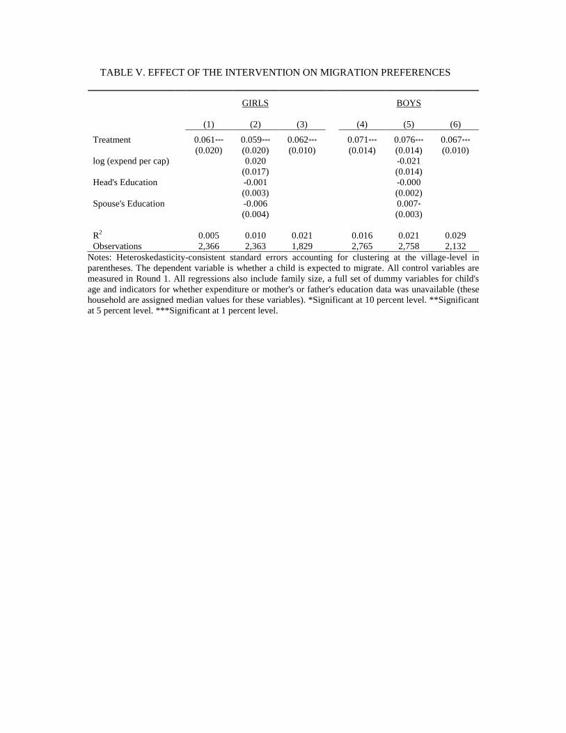
TABLE V. EFFECT OF THE INTERVENTION ON MIGRATION PREFERENCES

GIRLS

BOYS

(1) (2) (3) (4) (5) (6)

Treatment 0.061*** 0.059*** 0.062*** 0.071*** 0.076*** 0.067***

(0.020) (0.020) (0.010) (0.014) (0.014) (0.010)

log (expend per cap) 0.020 -0.021

(0.017) (0.014)

Head's Education -0.001 -0.000

(0.003) (0.002)

Spouse's Education -0.006 0.007*

(0.004) (0.003)

R2 0.005 0.010 0.021 0.016 0.021 0.029

Observations 2,366 2,363 1,829 2,765 2,758 2,132

Notes: Heteroskedasticity-consistent standard errors accounting for clustering at the village-level in

parentheses. The dependent variable is whether a child is expected to migrate. All control variables are

measured in Round 1. All regressions also include family size, a full set of dummy variables for child's

age and indicators for whether expenditure or mother's or father's education data was unavailable (these

household are assigned median values for these variables). *Significant at 10 percent level. **Significant

at 5 percent level. ***Significant at 1 percent level.

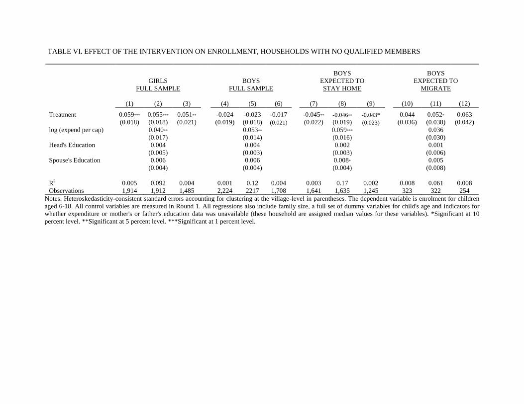
TABLE VI. EFFECT OF THE INTERVENTION ON ENROLLMENT, HOUSEHOLDS WITH NO QUALIFIED MEMBERS

GIRLS

FULL SAMPLE

BOYS

FULL SAMPLE

BOYS

EXPECTED TO

STAY HOME

BOYS

EXPECTED TO

MIGRATE

(1) (2) (3) (4) (5) (6) (7) (8) (9) (10) (11) (12)

Treatment 0.059*** 0.055*** 0.051** -0.024 -0.023 -0.017 -0.045** -0.046** -0.043* 0.044 0.052* 0.063

(0.018) (0.018) (0.021) (0.019) (0.018) (0.021) (0.022) (0.019) (0.023) (0.036) (0.038) (0.042)

log (expend per cap) 0.040** 0.053** 0.059*** 0.036

(0.017) (0.014) (0.016) (0.030)

Head's Education 0.004 0.004 0.002 0.001

(0.005) (0.003) (0.003) (0.006)

Spouse's Education 0.006 0.006 0.008* 0.005

(0.004) (0.004) (0.004) (0.008)

R2 0.005 0.092 0.004 0.001 0.12 0.004 0.003 0.17 0.002 0.008 0.061 0.008

Observations 1,914 1,912 1,485 2,224 2217 1,708 1,641 1,635 1,245 323 322 254

Notes: Heteroskedasticity-consistent standard errors accounting for clustering at the village-level in parentheses. The dependent variable is enrolment for children

aged 6-18. All control variables are measured in Round 1. All regressions also include family size, a full set of dummy variables for child's age and indicators for

whether expenditure or mother's or father's education data was unavailable (these household are assigned median values for these variables). *Significant at 10

percent level. **Significant at 5 percent level. ***Significant at 1 percent level.

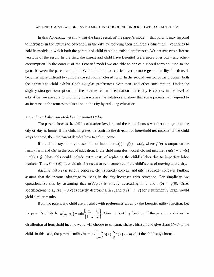
APPENDIX A: STRATEGIC INVESTMENT IN SCHOOLING UNDER BILATERAL ALTRUISM

In this Appendix, we show that the basic result of the paper‟s model – that parents may respond

to increases in the returns to education in the city by reducing their children‟s education – continues to

hold in models in which both the parent and child exhibit altruistic preferences. We present two different

versions of the result. In the first, the parent and child have Leontief preferences over own- and other-

consumption. In the context of the Leontief model we are able to derive a closed-form solution to the

game between the parent and child. While the intuition carries over to more general utility functions, it

becomes more difficult to compute the solution in closed form. In the second version of the problem, both

the parent and child exhibit Cobb-Douglas preferences over own- and other-consumption. Under the

slightly stronger assumption that the relative return to education in the city is convex in the level of

education, we are able to implicitly characterize the solution and show that some parents will respond to

an increase in the returns to education in the city by reducing education.

A.I: Bilateral Altruism Model with Leontief Utility

The parent chooses the child‟s education level, e, and the child chooses whether to migrate to the

city or stay at home. If the child migrates, he controls the division of household net income. If the child

stays at home, then the parent decides how to split income.

If the child stays home, household net income is h(e) = f(e) – c(e), where f (e) is output on the

family farm and c(e) is the cost of education. If the child migrates, household net income is m(e) = θ w(e)

– c(e) + f0. Note: this could include extra costs of replacing the child‟s labor due to imperfect labor

markets. Thus, f 0 ≤ f (0). It could also be recast to be income net of the child‟s cost of moving to the city.

Assume that f(e) is strictly concave, c(e) is strictly convex, and m(e) is strictly concave. Further,

assume that the income advantage to living in the city increases with education. For simplicity, we

operationalize this by assuming that h(e)/g(e) is strictly decreasing in e and h(0) > g(0). Other

specifications, e.g., h(e) – g(e) is strictly decreasing in e, and g(e) > h (e) for e sufficiently large, would

yield similar results.

Both the parent and child are altruistic with preferences given by the Leontief utility function. Let

the parent‟s utility be , min ,1

pkk p

xxu x x

s s

. Given this utility function, if the parent maximizes the

distribution of household income w, he will choose to consume share s himself and give share (1−s) to the

child. In this case, the parent‟s utility is 1

min ,1

s sh e h e h e

s s

if the child stays home.

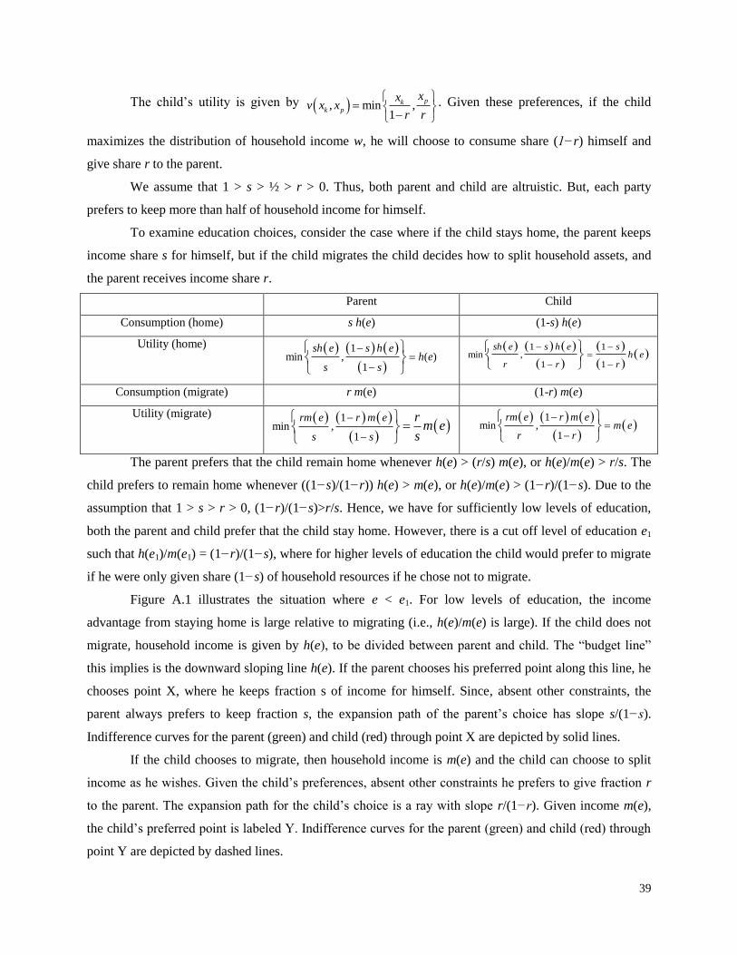
39

The child‟s utility is given by , min ,1

pkk p

xxv x x

r r

. Given these preferences, if the child

maximizes the distribution of household income w, he will choose to consume share (1−r) himself and

give share r to the parent.

We assume that 1 > s > ½ > r > 0. Thus, both parent and child are altruistic. But, each party

prefers to keep more than half of household income for himself.

To examine education choices, consider the case where if the child stays home, the parent keeps

income share s for himself, but if the child migrates the child decides how to split household assets, and

the parent receives income share r.

Parent Child

Consumption (home) s h(e) (1-s) h(e)

Utility (home)

1min , ( )

1

sh e s h eh e

s s

1 1min ,

1 1

sh e s h e sh e

r r r

Consumption (migrate) r m(e) (1-r) m(e)

Utility (migrate)

1min ,

1

rm e r m e

s s

rm e

s

1min ,

1

rm e r m em e

r r

The parent prefers that the child remain home whenever h(e) > (r/s) m(e), or h(e)/m(e) > r/s. The

child prefers to remain home whenever ((1−s)/(1−r)) h(e) > m(e), or h(e)/m(e) > (1−r)/(1−s). Due to the

assumption that 1 > s > r > 0, (1−r)/(1−s)>r/s. Hence, we have for sufficiently low levels of education,

both the parent and child prefer that the child stay home. However, there is a cut off level of education e1

such that h(e1)/m(e1) = (1−r)/(1−s), where for higher levels of education the child would prefer to migrate

if he were only given share (1−s) of household resources if he chose not to migrate.

Figure A.1 illustrates the situation where e < e1. For low levels of education, the income

advantage from staying home is large relative to migrating (i.e., h(e)/m(e) is large). If the child does not

migrate, household income is given by h(e), to be divided between parent and child. The “budget line”

this implies is the downward sloping line h(e). If the parent chooses his preferred point along this line, he

chooses point X, where he keeps fraction s of income for himself. Since, absent other constraints, the

parent always prefers to keep fraction s, the expansion path of the parent‟s choice has slope s/(1−s).

Indifference curves for the parent (green) and child (red) through point X are depicted by solid lines.

If the child chooses to migrate, then household income is m(e) and the child can choose to split

income as he wishes. Given the child‟s preferences, absent other constraints he prefers to give fraction r

to the parent. The expansion path for the child‟s choice is a ray with slope r/(1−r). Given income m(e),

the child‟s preferred point is labeled Y. Indifference curves for the parent (green) and child (red) through

point Y are depicted by dashed lines.

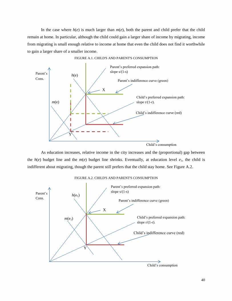
40

In the case where h(e) is much larger than m(e), both the parent and child prefer that the child

remain at home. In particular, although the child could gain a larger share of income by migrating, income

from migrating is small enough relative to income at home that even the child does not find it worthwhile

to gain a larger share of a smaller income.

FIGURE A.1. CHILD'S AND PARENT'S CONSUMPTION

As education increases, relative income in the city increases and the (proportional) gap between

the h(e) budget line and the m(e) budget line shrinks. Eventually, at education level e1, the child is

indifferent about migrating, though the parent still prefers that the child stay home. See Figure A.2.

FIGURE A.2. CHILD'S AND PARENT'S CONSUMPTION

Child‟s consumption

Parent‟s

Cons.

Parent‟s preferred expansion path:

slope s/(1-s)

Child‟s preferred expansion path:

slope r/(1-r).

Parent‟s indifference curve (green)

Child‟s indifference curve (red)

h(e1)

m(e1)

X

Y

Child‟s consumption

Parent‟s

Cons.

Parent‟s preferred expansion path:

slope s/(1-s)

Child‟s preferred expansion path:

slope r/(1-r).

Parent‟s indifference curve (green)

Child‟s indifference curve (red)

h(e)

m(e)

X

Y

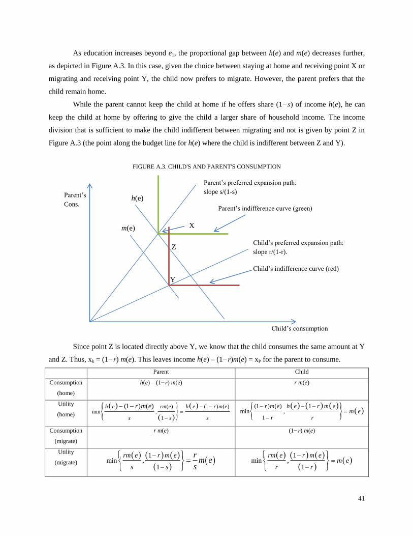
41

As education increases beyond e1, the proportional gap between h(e) and m(e) decreases further,

as depicted in Figure A.3. In this case, given the choice between staying at home and receiving point X or

migrating and receiving point Y, the child now prefers to migrate. However, the parent prefers that the

child remain home.

While the parent cannot keep the child at home if he offers share (1−s) of income h(e), he can

keep the child at home by offering to give the child a larger share of household income. The income

division that is sufficient to make the child indifferent between migrating and not is given by point Z in

Figure A.3 (the point along the budget line for h(e) where the child is indifferent between Z and Y).

FIGURE A.3. CHILD'S AND PARENT'S CONSUMPTION

Since point Z is located directly above Y, we know that the child consumes the same amount at Y

and Z. Thus, xk = (1−r) m(e). This leaves income h(e) – (1−r)m(e) = xP for the parent to consume.

Parent Child

Consumption

(home)

h(e) – (1−r) m(e) r m(e)

Utility

(home)

( ) (1 ) ( )min ,

1

(1 ) ( )h e rm e h e r m e

s s s

r m e

(1 ) ( ) 1

min ,1

r m e h e r m em e

r r

Consumption

(migrate)

r m(e) (1−r) m(e)

Utility

(migrate)

1min ,

1

rm e r m e

s s

rm e

s

1min ,

1

rm e r m em e

r r

Child‟s consumption

Parent‟s

Cons.

Parent‟s preferred expansion path:

slope s/(1-s)

Child‟s preferred expansion path:

slope r/(1-r).

Parent‟s indifference curve (green)

Child‟s indifference curve (red)

h(e)

m(e) X

Y

Z

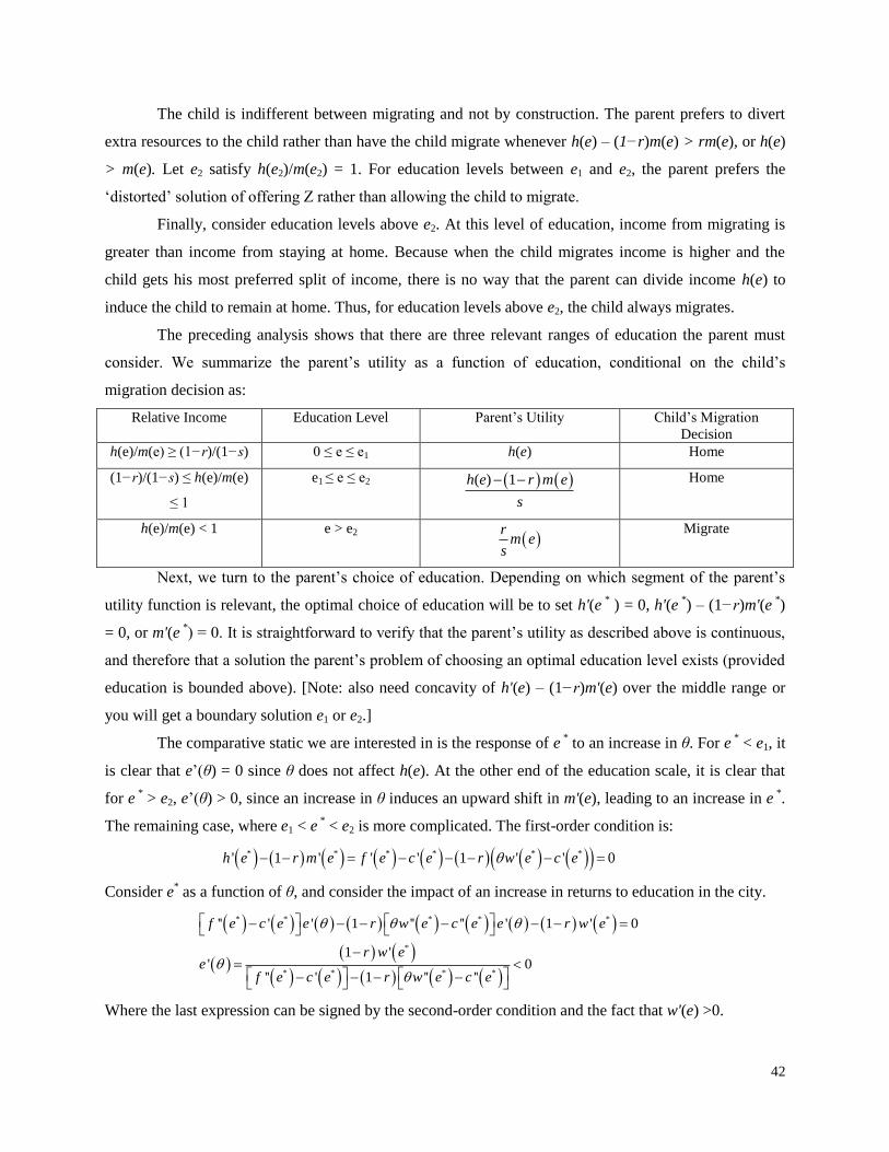
42

The child is indifferent between migrating and not by construction. The parent prefers to divert

extra resources to the child rather than have the child migrate whenever h(e) – (1−r)m(e) > rm(e), or h(e)

> m(e). Let e2 satisfy h(e2)/m(e2) = 1. For education levels between e1 and e2, the parent prefers the

„distorted‟ solution of offering Z rather than allowing the child to migrate.

Finally, consider education levels above e2. At this level of education, income from migrating is

greater than income from staying at home. Because when the child migrates income is higher and the

child gets his most preferred split of income, there is no way that the parent can divide income h(e) to

induce the child to remain at home. Thus, for education levels above e2, the child always migrates.

The preceding analysis shows that there are three relevant ranges of education the parent must

consider. We summarize the parent‟s utility as a function of education, conditional on the child‟s

migration decision as:

Relative Income Education Level Parent‟s Utility Child‟s Migration

Decision

h(e)/m(e) ≥ (1−r)/(1−s) 0 ≤ e ≤ e1 h(e) Home

(1−r)/(1−s) ≤ h(e)/m(e)

≤ 1

e1 ≤ e ≤ e2 ( ) 1h e r m e

s

Home

h(e)/m(e) < 1 e > e2

rm e

s

Migrate

Next, we turn to the parent‟s choice of education. Depending on which segment of the parent‟s

utility function is relevant, the optimal choice of education will be to set h'(e * ) = 0, h'(e

*) – (1−r)m'(e

*)

= 0, or m'(e *) = 0. It is straightforward to verify that the parent‟s utility as described above is continuous,

and therefore that a solution the parent‟s problem of choosing an optimal education level exists (provided

education is bounded above). [Note: also need concavity of h'(e) – (1−r)m'(e) over the middle range or

you will get a boundary solution e1 or e2.]

The comparative static we are interested in is the response of e * to an increase in θ. For e

* < e1, it

is clear that e‟(θ) = 0 since θ does not affect h(e). At the other end of the education scale, it is clear that

for e * > e2, e‟(θ) > 0, since an increase in θ induces an upward shift in m'(e), leading to an increase in e

*.

The remaining case, where e1 < e * < e2 is more complicated. The first-order condition is:

* * * * * *' 1 ' ' ' 1 ' ' 0h e r m e f e c e r w e c e

Consider e* as a function of θ, and consider the impact of an increase in returns to education in the city.

* * * * *

*

* * * *

'' ' ' 1 '' '' ' 1 ' 0

1 '' 0

'' ' 1 '' ''

f e c e e r w e c e e r w e

r w ee

f e c e r w e c e

Where the last expression can be signed by the second-order condition and the fact that w'(e) >0.

43

Hence we have for education levels in the range where the parent must divert additional resources

to the child in order to keep him from choosing to migrate, and increase in the returns to education in the

city induces the parent to reduce the child‟s education. The intuition is straightforward. When the parent

chooses education levels over this range, he weighs the marginal benefit from increasing income against

the marginal cost of education and the fact that at higher education levels migration becomes more

attractive, and the parent must give the child additional resources because of this. Thus, this additional

transfer behaves as an additional marginal cost of education – the marginal incentive cost of education.

An increase in θ increases the rate at which the attractiveness of migration increases for the child, and

thus increases the parent‟s marginal incentive cost of increasing the child‟s education. The result is that

the parent chooses to lower the education given to the child in order to reduce their temptation to migrate.

Note that an increase in θ will decrease e1 and e2.

For given functions h(e) and m(e), the optimal education choice will be in one of the regions

described above. Which region the solution lies in will depend on h(e) and m(e). Thus, one needs to check

for possible solutions in each of the regions and compare the parent‟s utility in each case. Note, however,

that if there is a level of education e such that h'(e) = 0 and e ≤ e1, then there cannot be an e with e1 ≤ e ≤

e2 and h'(e) – (1−r)m'(e). Similarly, existence of a solution to h'(e) – (1−r) m'(e) = 0 with e1 ≤ e ≤ e2

precludes a solution to h'(e) = 0 with e ≤ e1. Hence, there can be a candidate solution with e ≤ e1 or e1 ≤ e

≤ e2, but not both. If there exists an education level with m'(e) = 0 and e ≥ e2, then the optimal educational

choice is given by comparing the parent‟s utility under the (at most) two candidate optimal solutions.

For simplicity, assume that h'(e1) > 0, so that solutions with e ≤ e1 are not relevant. Suppose there

exists education level e* such that h'(e

*) – (1−r)m'(e

*) = 0 and e1 ≤ e ≤ e2 and education level e

** such that

m'(e**

) = 0. The parent‟s utility in the two cases are proportional to h(e*) – (1−r)m(e

*) and r m(e

**),

respectively. It is better to choose e* than e

** whenever h(e

*) – (1−r) m(e

*) > r m(e

**), or h(e

* ) > r m(e

**)

+ (1−r) m(e*).

The above condition holds for any particular household. To get a sense of which households will

choose to have children migrate, we introduce heterogeneity into the households. In particular, recall that

m(e) = θ w(e) – c(e) +f0, where f0 captures the (optimized) profit of the household farm if the child moves

away. The term f0 can be heterogeneous across households and capture idiosyncratic differences in the

cost of replacing the child‟s household inputs and contributions to home produced goods as well as any

transition costs the child may have from moving to the city. When f0 is high, it corresponds to situations

where the idiosyncratic cost of losing the child to the city is low, while when f0 is low, this corresponds to

situations where the idiosyncratic cost of losing the child to the city is high.

Since f0 does not affect the marginal returns to education, e* and e

** are unaffected by changed in

f0. On the other hand, an increase in f0 decreases e2 and increases m(e). Both of these factors make it more

44

likely that households with high f0 will find it optimal to allow their children to migrate. In particular,

there exists a cut-off level of f0, F, such that if f0 < F, it is optimal for the household to choose e = e* and

keep the child at home, while if f0 > F, it is optimal for the household to choose e = e**

and have the child

choose to migrate.

Now, consider a household with f0 = F. Such a household has h(e*) − (1−r) m(e

*) = r m(e

**). By

the envelope theorem, an increase in θ decreases the left-hand side of the equation and increases the right-

hand side. Thus, a household that is indifferent between migrating and not before the increase in θ strictly

prefers migration after. This is because the increase in θ both increases income in the city and increases

the incentive cost of keeping the child home.

Overall, the above establishes that in response to an increase in the city returns to education:

1. Parents who prefer their children to migrate will give their children more education,

2. Parents who prefer their children to stay home will either leave education unchanged or decrease it,

3. More parents will prefer their children to migrate.

A.II: Cobb-Douglas Preferences

As in the previous versions, the parent chooses the child‟s education level, e, and the child

chooses whether to migrate to the city or stay at home. If the child migrates, he controls the division of

household net income. If the stays at home, then the parent decides how to split income.

If the child stays home, household net income is h(e) = f(e) – c(e), where f(e) is output on the

family farm and c(e) is the cost of education. If the child migrates, household net income is m(e) = θ w(e)

– c(e) + f0. Note: this could include extra costs of replacing the child‟s labor due to imperfect labor

markets. Thus, f0 ≤ f(0) is possible. It could also be recast to be income net of the child‟s cost of moving

to the city.

Assume that f(e) is strictly concave, c(e) is strictly convex, that m(e) is strictly concave. Further,

assume that the income advantage to living in the city increases with education. For simplicity, we

operationalize this assumption by assuming that h(e)/g(e) is strictly decreasing in e and h(0) > g(0). Other

specifications, e.g., h(e) – g(e) is strictly decreasing in e, and g(e) > h(e) for e sufficiently large, would

yield similar results.

Child‟s Utility: v(xk,xp) = xk1-r

xpr where xk and xp are the child‟s consumption expenditure and the

parent‟s, respectively.

Parent‟s Utility: u(xp,xk) = xk1-s

xps , where xk and xp are the child‟s consumption expenditure and the

parent‟s, respectively.

45

We assume that r < s, so that the child places more value on the child‟s consumption than the

parent does. A stronger assumption, r < ½ < s, would imply that each party is altruistic but places greater

weight on own consumption than the other party‟s. However, the less restrictive assumption is sufficient

for the results.

Child‟s Problem. Suppose the child chooses xk and xp to solve:

,max ( , )

. .

k px x k p

k p

v x x

s t x x w

The solution to this problem is:

1k px w r w and x w rw ,

and the corresponding indirect utility function is v(w) = A w, where A = rr(1−r)

1−r.

Parent‟s Problem. Suppose the parent chooses xk and xp to solve:

,max ( , )

. .

k px x k p

k p

u x x

s t x x w

The solution to this problem is:

1k px w s w and x w sw ,

and the corresponding indirect utility function is u(w) = b w, where b = ss(1−s)

1−s.

Finally, it will be useful to define two quantities. Suppose that the parent chooses to split income

giving share s to himself and share (1−s) to the child. The child‟s utility from this is given by:

1

1 , 1r rv s w sw s s w aw

.

Since the child‟s preferred split of income earns higher utility when income is w, we have that A

> a. Similarly, when the child chooses to split income keeping share (1−r) for himself and giving share r

to the parent, the parent‟s utility is

1

1 , 1 ,s su r w rw r r w bw

where by the same argument B > b.

To examine education choices, consider the case where, if the child stays home, the parent keeps

income share s for himself, but if the child migrates, the child decides how to split household assets and

the parent receives income share r.

Parent Child

Consumption (home) s h(e) (1−s) h(e)

Utility (home) B h(e) a h(e)

Consumption (migrate) r m(e) (1−r) m(e)

Utility (migrate) b m(e) A m(e)

46

The parent prefers that the child stay home whenever B h(e) > b m(e), or h(e)/m(e) > b/B. The

child prefers to remain home whenever ah(e) > A m(e), or h(e)/m(e) > A/a. Since A > a and b < B, we

have that there is a range of education levels, b/B < h(e)/m(e) < A/a where the parent prefers that the child

stay home but the child prefers to migrate.

Education can therefore be divided into three regions. For e < e1, where h(e1)/m(e1) = A/a, both

the parent and child prefer that the child remain home. For e1 ≤ e ≤ e2, where h(e2)/m(e2) = b/B, the parent

prefers the child to remain home but the child prefers to migrate. For e > e2, both the parent and child

prefer that the child migrate.

Let us focus for the moment on the case where e1 ≤ e ≤ e2. In this case, if the parent chooses to

give the child share (1−s) of income, the child will choose to migrate to the city. However, the parent can

induce the child to remain at home by giving him a greater share of household resources. Although the

parent is worse off relative to the case where the parent can keep share s of household wealth for himself,

the parent may find this preferable to allowing the child to migrate and receiving share r.

Holding fixed the choice of e, the parent‟s problem can be written as:

1

,

1

max

. .

k p

s s

x x k p

k p

r r

k p

x x

s t x x h e

x x Bm e

The solution to this problem satisfies the two constraints.

We can simplify the problem as follows. First, let xk = (1−t) h(e) and xp = t h(e). In this case, the

first constraint can be eliminated, and we rewrite the problem as:

1

1

max 1

. . 1

r r

s s

t h e th e

s t t h e th e Bm e

This in turn becomes:

1

1

max 1

. . 1

r r

s s

h e t t

s t h e t t Bm e

And one more small step gives:

1

1

max 1

. . 1

r r

s s

h e t t

h es t t t B

m e

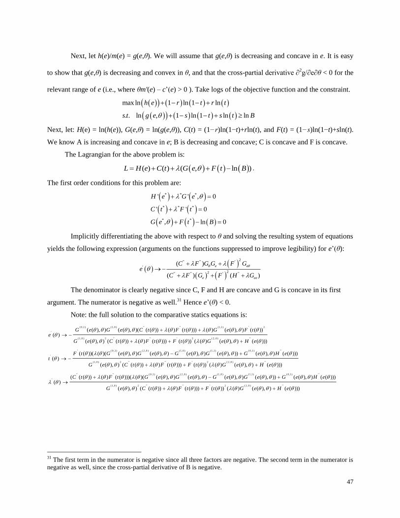
47

Next, let h(e)/m(e) = g(e,θ). We will assume that g(e,θ) is decreasing and concave in e. It is easy

to show that g(e,θ) is decreasing and convex in θ, and that the cross-partial derivative ∂2g/∂e∂θ < 0 for the

relevant range of e (i.e., where θm'(e) – c‟(e) > 0 ). Take logs of the objective function and the constraint.

max ln 1 ln 1 ln

. . ln , 1 ln 1 ln ln

h e r t r t

s t g e s t s t B

Next, let: H(e) = ln(h(e)), G(e,θ) = ln(g(e,θ)), C(t) = (1−r)ln(1−t)+rln(t), and F(t) = (1−s)ln(1−t)+sln(t).

We know A is increasing and concave in e; B is decreasing and concave; C is concave and F is concave.

The Lagrangian for the above problem is:

( ) ( ) ( , ln )L H e C t G e F t B .

The first order conditions for this problem are:

* * *

* * *

* *

' ' , 0

' ' 0

, ln 0

H e G e

C t F t

G e F t B

Implicitly differentiating the above with respect to θ and solving the resulting system of equations

yields the following expression (arguments on the functions suppressed to improve legibility) for e‟(θ):

2

22

( )

( ) ( )

e e

e ee

C F G G F Ge

C F G F H G

The denominator is clearly negative since C, F and H are concave and G is concave in its first

argument. The numerator is negative as well.31

Hence e‟(θ) < 0.

Note: the full solution to the comparative statics equations is:

( 0 ,1) (1,0 ) (1,1) 2

(1,0 ) 2 2 ( 2 ,0 )

( 0 ,1)

( ( ), ) ( ( ), )( ( ( )) ( ) ( ( ))) ( ) ( ( ), ) ( ( ))( )

( ( ), ) ( ( ( )) ( ) ( ( ))) ( ( )) ( ( ) ( ( ), ) ( ( )))

( ( ))( ( )( ( ( )( )

G e G e C t F t G e F te

G e C t F t F t G e H e

F t G et

( 2 ,0 ) (1,0 ) (1,1) ( 0 ,1)

(1,0 ) 2 2 ( 2 ,0 )

( 0 ,1)

, ) ( ( ), ) ( ( ), ) ( ( ), )) ( ( ), ) ( ( )))

( ( ), ) ( ( ( )) ( ) ( ( ))) ( ( )) ( ( ) ( ( ), ) ( ( )))

( ( ( )) ( ) ( ( )))( ( )( ( ( )( )

G e G e G e G e H e

G e C t F t F t G e H e

C t F t G e

( 2 ,0 ) (1,0 ) (1,1) ( 0 ,1)

(1,0 ) 2 2 ( 2 ,0 )

, ) ( ( ), ) ( ( ), ) ( ( ), )) ( ( ), ) ( ( )))

( ( ), ) ( ( ( )) ( ) ( ( ))) ( ( )) ( ( ) ( ( ), ) ( ( )))

G e G e G e G e H e

G e C t F t F t G e H e

31

The first term in the numerator is negative since all three factors are negative. The second term in the numerator is

negative as well, since the cross-partial derivative of B is negative.

48

APPENDIX B: THE CASE OF MULTIPLE CHILDREN

Suppose the parent has N children, numbered 1, …, N with generic element n. The parent chooses

education level ei for each child. The cost of education is c(e), where c' > 0 and c'' ≥ 0. Let H be the set of

children the parent wishes to stay home and M be the set of children that the parent wishes to migrate.

With slight abuse of notation, we will use H and M to denote the number of children in each set when it

can be done without confusion.

Let FH(e1,…,eH) denote the household production function when set H of children remain at

home. Children who migrate to the city earn wage w(e) and remit fraction r home to the parent, where 0 ≤

r ≤ 1. The cost of migrating to the city is t > 0. We assume it is the same for all children, but that can be

relaxed. We can also include a child-specific value ui that the parent assigns to keeping the child at home.

For a child the parent wishes to keep at home, the parent must offer that child as much net income

as the child would receive if the child were to migrate. If the child remits fraction r of income home to the

parent, his net income is vi = (1−r) w(ei) – t.

The parent chooses household income subject to the constraint that children who remain at home

are willing to do so:

, , 1 1max ,...,

. .

1

i

N

H M e H H m n hm M n h H

h h

F e e rw e c e x

s t

x r w e t for all h H

Substituting the constraints into the objective function yields:

, , 1 1max ,..., 1

i

N

H M e H H m n hm M n h HF e e rw e c e r w e t

An optimal (interior) solution to this problem satisfies:

* * *

* * * * *

1

' '

,..., ' 1 '

m m

H h h

h

rw e c e for m M

Fe e c e r w e for h H

e

The comparative static we are interested in is how the optimal choice of education changes when there is

a change in the marginal returns to education in the city. To illustrate this, rewrite the wage function as z

w(e). We will analyze the impact of an increase in z on the solution to the parent‟s problem, now

characterized by:

* * *

* * * * *

1

' '

,..., ' 1 '

m m

H h h

h

rzw e c e for m M

Fe e c e r zw e for h H

e

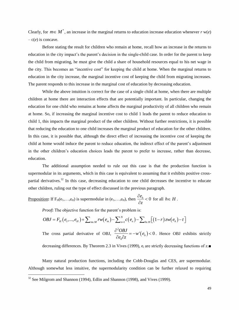
49

Clearly, for *m M , an increase in the marginal returns to education increase education whenever r w(e)

– c(e) is concave.

Before stating the result for children who remain at home, recall how an increase in the returns to

education in the city impact‟s the parent‟s decision in the single-child case. In order for the parent to keep

the child from migrating, he must give the child a share of household resources equal to his net wage in

the city. This becomes an “incentive cost” for keeping the child at home. When the marginal returns to

education in the city increase, the marginal incentive cost of keeping the child from migrating increases.

The parent responds to this increase in the marginal cost of education by decreasing education.

While the above intuition is correct for the case of a single child at home, when there are multiple

children at home there are interaction effects that are potentially important. In particular, changing the

education for one child who remains at home affects the marginal productivity of all children who remain

at home. So, if increasing the marginal incentive cost to child 1 leads the parent to reduce education to

child 1, this impacts the marginal product of the other children. Without further restrictions, it is possible

that reducing the education to one child increases the marginal product of education for the other children.

In this case, it is possible that, although the direct effect of increasing the incentive cost of keeping the

child at home would induce the parent to reduce education, the indirect effect of the parent‟s adjustment

in the other children‟s education choices leads the parent to prefer to increase, rather than decrease,

education.

The additional assumption needed to rule out this case is that the production function is

supermodular in its arguments, which in this case is equivalent to assuming that it exhibits positive cross-

partial derivatives.32

In this case, decreasing education to one child decreases the incentive to educate

other children, ruling out the type of effect discussed in the previous paragraph.

Proposition: If FH(e1,…,eH) is supermodular in (e1,…,eH), then 0he

z

for all h H .

Proof: The objective function for the parent‟s problem is:

1 1,..., 1

N

H H m n hm M n h HOBJ F e e rw e c e r zw e t

The cross partial derivative of OBJ, 2

' 0h

h

OBJw e

e z

. Hence OBJ exhibits strictly

decreasing differences. By Theorem 2.3 in Vives (1999), ei are strictly decreasing functions of z.■

Many natural production functions, including the Cobb-Douglas and CES, are supermodular.

Although somewhat less intuitive, the supermodularity condition can be further relaxed to requiring

32

See Milgrom and Shannon (1994), Edlin and Shannon (1998), and Vives (1999).

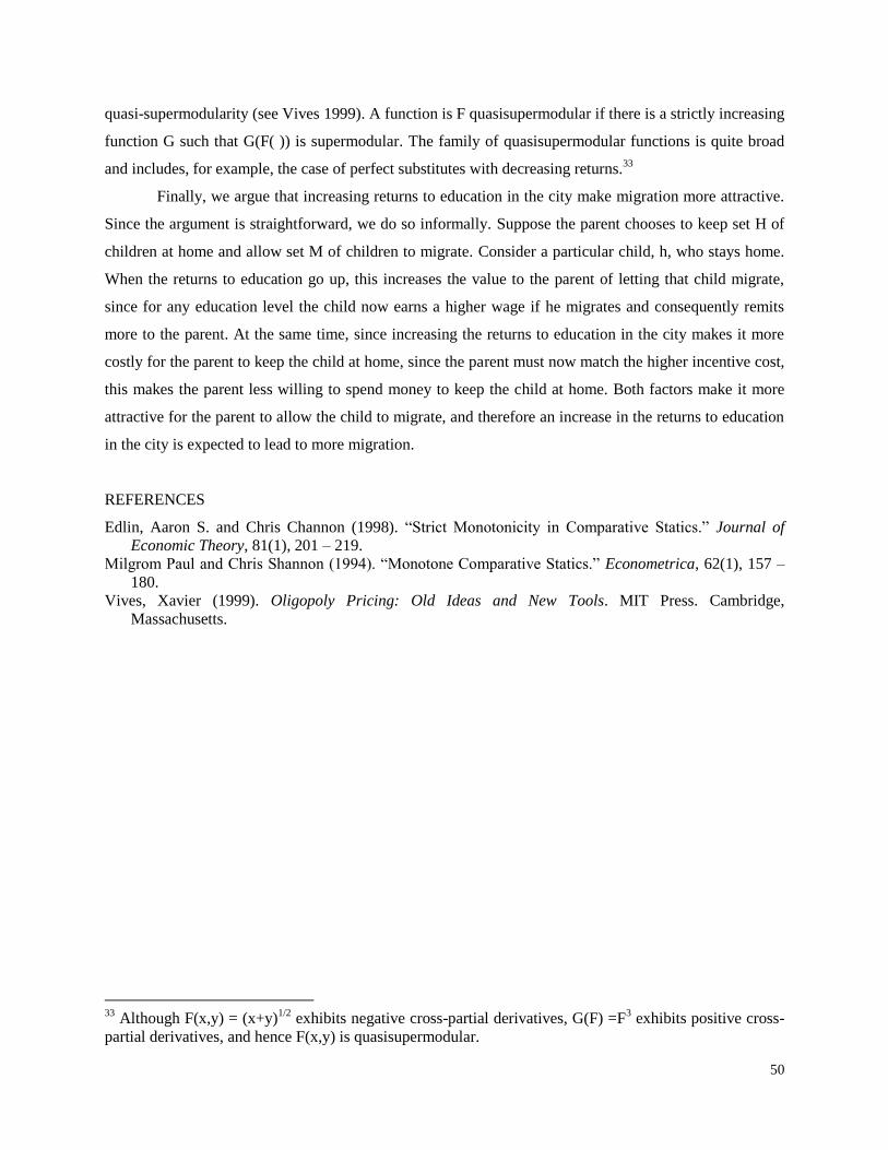
50

quasi-supermodularity (see Vives 1999). A function is F quasisupermodular if there is a strictly increasing

function G such that G(F( )) is supermodular. The family of quasisupermodular functions is quite broad

and includes, for example, the case of perfect substitutes with decreasing returns.33

Finally, we argue that increasing returns to education in the city make migration more attractive.

Since the argument is straightforward, we do so informally. Suppose the parent chooses to keep set H of

children at home and allow set M of children to migrate. Consider a particular child, h, who stays home.

When the returns to education go up, this increases the value to the parent of letting that child migrate,

since for any education level the child now earns a higher wage if he migrates and consequently remits

more to the parent. At the same time, since increasing the returns to education in the city makes it more

costly for the parent to keep the child at home, since the parent must now match the higher incentive cost,

this makes the parent less willing to spend money to keep the child at home. Both factors make it more

attractive for the parent to allow the child to migrate, and therefore an increase in the returns to education

in the city is expected to lead to more migration.

REFERENCES

Edlin, Aaron S. and Chris Channon (1998). “Strict Monotonicity in Comparative Statics.” Journal of

Economic Theory, 81(1), 201 – 219.

Milgrom Paul and Chris Shannon (1994). “Monotone Comparative Statics.” Econometrica, 62(1), 157 –

180.

Vives, Xavier (1999). Oligopoly Pricing: Old Ideas and New Tools. MIT Press. Cambridge,

Massachusetts.

33

Although F(x,y) = (x+y)1/2

exhibits negative cross-partial derivatives, G(F) =F3 exhibits positive cross-

partial derivatives, and hence F(x,y) is quasisupermodular.

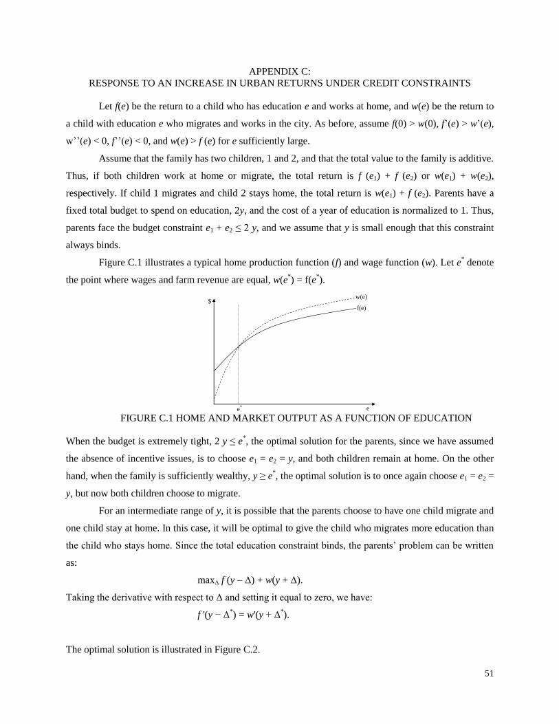
51

APPENDIX C:

RESPONSE TO AN INCREASE IN URBAN RETURNS UNDER CREDIT CONSTRAINTS

Let f(e) be the return to a child who has education e and works at home, and w(e) be the return to

a child with education e who migrates and works in the city. As before, assume f(0) > w(0), f‟(e) > w‟(e),

w‟‟(e) < 0, f‟‟(e) < 0, and w(e) > f (e) for e sufficiently large.

Assume that the family has two children, 1 and 2, and that the total value to the family is additive.

Thus, if both children work at home or migrate, the total return is f (e1) + f (e2) or w(e1) + w(e2),

respectively. If child 1 migrates and child 2 stays home, the total return is w(e1) + f (e2). Parents have a

fixed total budget to spend on education, 2y, and the cost of a year of education is normalized to 1. Thus,

parents face the budget constraint e1 + e2 ≤ 2 y, and we assume that y is small enough that this constraint

always binds.

Figure C.1 illustrates a typical home production function (f) and wage function (w). Let e* denote

the point where wages and farm revenue are equal, w(e*) = f(e

*).

f(e)

w(e)

e

$

e*

FIGURE C.1 HOME AND MARKET OUTPUT AS A FUNCTION OF EDUCATION

When the budget is extremely tight, 2 y ≤ e*, the optimal solution for the parents, since we have assumed

the absence of incentive issues, is to choose e1 = e2 = y, and both children remain at home. On the other

hand, when the family is sufficiently wealthy, y ≥ e*, the optimal solution is to once again choose e1 = e2 =

y, but now both children choose to migrate.

For an intermediate range of y, it is possible that the parents choose to have one child migrate and

one child stay at home. In this case, it will be optimal to give the child who migrates more education than

the child who stays home. Since the total education constraint binds, the parents‟ problem can be written

as:

maxΔ f (y – Δ) + w(y + Δ).

Taking the derivative with respect to Δ and setting it equal to zero, we have:

f '(y − Δ*) = w'(y + Δ

*).

The optimal solution is illustrated in Figure C.2.

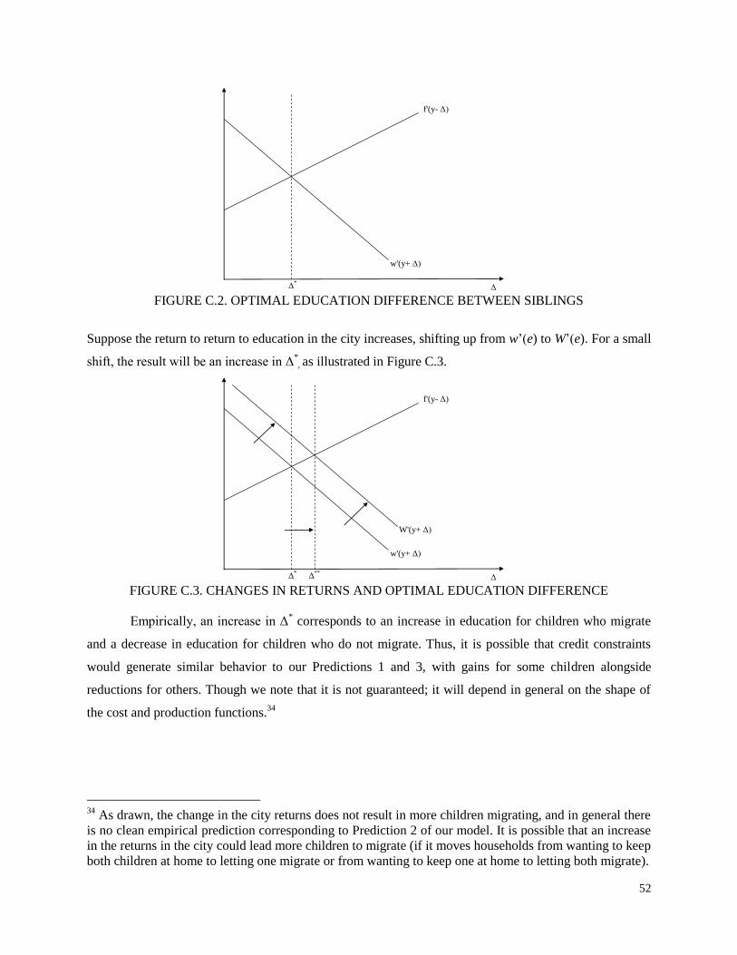
52

Δ

w'(y+ Δ)

f'(y- Δ)

Δ*

FIGURE C.2. OPTIMAL EDUCATION DIFFERENCE BETWEEN SIBLINGS

Suppose the return to return to education in the city increases, shifting up from w‟(e) to W‟(e). For a small

shift, the result will be an increase in Δ*, as illustrated in Figure C.3.

Δ

w'(y+ Δ)

f'(y- Δ)

Δ*

W'(y+ Δ)

Δ**

FIGURE C.3. CHANGES IN RETURNS AND OPTIMAL EDUCATION DIFFERENCE

Empirically, an increase in Δ* corresponds to an increase in education for children who migrate

and a decrease in education for children who do not migrate. Thus, it is possible that credit constraints

would generate similar behavior to our Predictions 1 and 3, with gains for some children alongside

reductions for others. Though we note that it is not guaranteed; it will depend in general on the shape of

the cost and production functions.34

34

As drawn, the change in the city returns does not result in more children migrating, and in general there

is no clean empirical prediction corresponding to Prediction 2 of our model. It is possible that an increase

in the returns in the city could lead more children to migrate (if it moves households from wanting to keep

both children at home to letting one migrate or from wanting to keep one at home to letting both migrate).