keller chen zhang forthcoming - columbia university

Observational Studies () Submitted ; Published

Heterogeneous Subgroup Identification with ObservationalData: A Case Study Based on the National Study of

Learning Mindsets

Bryan Keller [email protected] of Human DevelopmentTeachers College, Columbia UniversityNew York, NY 10027, USA

Jianshen Chen [email protected] GroupCollege BoardYardley, PA 19607, USA

Tianyang Zhang [email protected]

Department of Human Development

Teachers College, Columbia University

New York, NY 10027, USA

Abstract

In this paper, we use a two-step approach for heterogeneous subgroup identification witha synthetic data set motivated by the National Study of Learning Mindsets. In the firststep, optimal full propensity score matching is used to estimate stratum-specific treatmenteffects. In the second step, regression trees identify key subgroups based on covariates forwhich the treatment effect varies. In working with regression trees, we emphasize the roleof the cost-complexity tuning parameter, selected through permutation-based Type I errorrate studies, in justifying inferential decision-making, which we contrast with graphical andquantitative exploration for future study. Results indicate that the mindset interventionwas effective, overall, in improving student achievement. While our exploratory analysesidentified XC, C1, and X1 as potential effect modifiers worthy of further study, we findno statistically significant evidence of effect heterogeneity with the exception of urbanicitycategory XC = 3, but the finding is not robust to propensity score estimation method.

Keywords: Heterogeneous Treatment Effect, Observational Studies, Propensity ScoreMatching, Regression Trees

1. Methodology and Motivation

1.1 Introduction

Despite the overwhelming focus on the overall average treatment effect (ATE) in the statis-tics and causal inference literatures, there are many scenarios for which the efficacy of atreatment may vary depending on unit background characteristics. Methods that targetconditional average treatment effects can explain how pretreatment variables interact with

c© Bryan Keller, Jianshen Chen and Tianyang Zhang.

Keller, Chen and Zhang

treatment exposure to cause heterogeneity in treatment efficacy. The identification of suchheterogeneity, to the extent that it exists, is of tremendous interest to stakeholders because itcan provide insight into which types of participants are likely to be helped the most, helpedthe least, or even harmed by an intervention. In this paper, we begin with an overview of thesynthetic data set generated for the Workshop for Empirical Investigation of Methods forHeterogeneity, a workshop that co-occurred with the 2018 Meeting of the Atlantic CausalInference Conference in Pittsburgh, PA. We then describe our approach for heterogeneoussubgroup identification based on propensity score matching and regression trees. We thendiscuss data analysis results presented at the workshop, followed by the results of furtheranalyses conducted after the workshop. We conclude with some discussion.

1.2 The Data

The workshop data analyzed herein are synthetic, but were motivated by the National Studyof Learning Mindsets, a randomized controlled trial of an intervention designed to encouragea growth mindset in high school students (Mindset Scholars Network, 2018). Approximately10,000 cases, nested in 76 schools, were simulated to emulate an observational study basedon four categorical student-level covariates and six numeric school-level covariates.

The three research questions we were asked to address for the workshop are as follows:

1. Was the mindset intervention effective in improving student achievement?

2. X1 is a measure of the average fixed mindset rating for each school; X2 is a measure ofschool-level academic achievement; both were measured before the intervention. Re-searchers suspect either (a) the effect is largest in middle-achieving schools, or (b) theeffect is decreasing in school-level achievement. Is there any evidence that X1 and/orX2 moderate the effect of the intervention on student-level academic achievement?

3. Is there evidence that any other covariates moderate the intervention effect?

1.3 Notation

Let Y 1i and Y 0

i be the potential outcomes (Neyman, 1923; Rubin, 1974) under treatment(Zi = 1) and comparison (Zi = 0) conditions, respectively. The average treatment effect, orATE, is defined as the average of individual treatment effects; that is, ATE = E[Y 1

i − Y 0i ].

A conditional average treatment effect, or CATE, is defined as the average of individualtreatment effects, given that a vector of covariates Xi1, Xi2, . . . , Xip take on particularvalues; that is, CATE = E[Y 1

i − Y 0i |Xi1 = xi1, Xi2 = xi1, . . . , Xip = xip]. The propensity

score, ei(Xi) = pr(Zi = 1|Xi), is the probability that unit i is assigned to (or selects) thetreatment group, given the observed covariates. For identification of the ATE and CATE,propensity score analysis, and other conditioning strategies, rely on the strong ignorabilityassumption (Rosenbaum and Rubin, 1983), which specifies

1. ignorability : the potential outcomes are independent of the treatment assignmentgiven observed covariates X; that is, {Y 0, Y 1} ⊥⊥ Z|X,

2. reliable measurement : observed covariates X have been reliably measured (Steineret al., 2011), and

2

Heterogeneous Subgroup Identification with Observational Data

3. positivity : the propensity score for each unit lies strictly between zero and one; thatis, 0 < ei(Xi) < 1 for all i.

The observed outcome for unit i, Yi, is defined via the potential outcomes and thetreatment indicator as Yi = ZiY

1i + (1− Zi)Y

0i .

1.4 Methodology

Our approach to heterogeneous subgroup identification is based on the fact that, underignorability, X ⊥⊥ Z|e(X) (Rosenbaum and Rubin, 1983). That is, by conditioning onthe propensity score, balance on the observed covariates across treated and comparisongroups may be restored to what would have been expected in a randomized experiment;namely, covariate distributions are identical (in the limit) across groups. We use optimalfull propensity score matching to stratify units into S strata, each of which contains atleast one treated case and at least one comparison case. For each stratum s ∈ 1, . . . , S, theestimate of the stratum-specific treatment effect is calculated as the difference in sampleaverages, treated group minus comparison group. That is,

ˆATEs =1

nTs

∑i∈Ts

Yi −1

nCs

∑i∈Cs

Yi,

where Ts and Cs are, respectively, the sets of indices of the treated and comparison casesin stratum s, and nTs and nCs respectively represent the cardinalities of Ts and Cs. Oncestratum-specific treatment effect estimates have been calculated, we use those values asestimates of the individual treatment effect for each unit in the stratum. We then regress thevector of individual treatment effects on the set of predictors using a single regression tree.Any predictors identified by the regression tree as important, meaning that the regressiontree split on those variables, are interpreted as evidence for effect heterogeneity on thevariable or variables involved in the splits.

1.4.1 Regression Trees

A regression tree is an algorithmic method invented by Breiman et al. (1984) that models theresponse surface for an outcome variable, Y , based on predictors, X1, . . . , Xp, by iterativelysplitting units into subgroups based on rectangular regions of predictor values. At eachiteration, a split creates two subgroups, called nodes, and a node that has not been splitis referred to as a terminal node. The predicted value based on the regression tree for anyunit in a terminal node is simply the mean score on the outcome variable for all units inthat node. For unit i in terminal node t, where Nt represents the set of units in t, thetree-predicted value for unit i is simply the mean score on the outcome variable for all units

in that node: Yi = 1|Nt|

∑i∈Nt

Yi. The deviance for a tree T , dev(T ) =∑

i

(Yi − Yi

)2, is

used as a cost function to determine the split point at each iteration. After considering allpossible splits on all possible variables, the split that yields the largest decrease in devianceis selected.

If left unchecked, regression trees would continue to split until each terminal node con-tained only one point. A commonly used approach to prevent this kind of overfitting isbased on adding a term to the squared error that penalizes the number of terminal nodes,

3


|T |, in tree T : C(T )cp = dev(T ) + cp|T |. This approach is referred to as cost-complexitypruning, and is implemented in the rpart package (Therneau et al., 2015) in R (R CoreTeam, 2018), which we use to fit regression trees. The tuning parameter, cp, is analogousto the smoothing parameter in the lasso or regularized regression, and is typically selectedthrough cross-validation.

2. Workshop Results

In the synthetic workshop data, school sample sizes for the 76 schools ranged from 14 to529, with a median of 111, and a mean of 136.7. Furthermore, the treatment was non-randomly assigned within schools, such that each school sample contained a proportion oftreated cases that ranged from about 17% to about 45%. This design feature allowed usto estimate propensity scores and create matches within schools1. As a result of within-school matching, all were matched exactly on the five continuously measured school-levelcovariates, X1, . . . , X5. For the workshop, we used two methods to estimate propensityscores: random forests (RF) and generalized boosted modeling (GBM). Both methods arebased on regression trees and, therefore, algorithmically handle interactions and nonlinearrelationships.

2.1 Research Question 1

To address the first question, we used standard propensity score methodology and simplytook weighted averages of stratum-specific treatment effect estimates. The overall ATEwas estimated to be 0.25 or 0.26, based on GBM or RF, respectively, for propensity scoreestimation. The distribution of estimated individual treatment effects, along with a verticalline denoting the average, is shown for the RF analysis in Figure 1. While the resultssuggest a positive treatment effect, we did not present standard errors, so we made noclaims regarding evidence for an overall effect.


We fit regression trees and varied the level of the complexity parameter to search for het-erogeneity on X1 and X2. With analyses based on propensity scores estimated by RF andGBM, we noted, based on the regression tree output shown in Figure 2, that the treatmenteffect did appear to vary with X2 and X1.

Figure 2 shows the results of a regression tree fit based on random forests with a com-plexity parameter of 0.0033. Note that at the root node, the overall ATE is estimatedto be 0.26 based on 8910 cases. The first split was at X2 = −0.71, which led to condi-tional ATE estimates of ˆCATE{X2<−0.71} = 0.12 and ˆCATE{X2≥−0.71} = 0.29. The nextsplit was also on X2, thereby modeling a quadratic relationship. In particular, we see that

ˆCATE{X2≥0.83} = 0.23 and ˆCATE{−0.71<X2≤0.83} = 0.31. In other words, the estimatedaverage treatment effect for schools with academic achievement scores between -0.71 and0.83 was 0.31, higher than the estimate of 0.12 for schools with pretest achievement below-0.71, and higher than the estimate of 0.23 for schools with pretest achievement above 0.83.

1. Note, however, that two schools, numbers 11 and 31, were dropped due to insufficient sample sizes of 21and 14, respectively

4


Figure 1: Average Treatment Effect Estimate by the Random Forest (RF) Method

Figure 2: Regression Tree Based on Regressing Individual Treatment Effect Estimates onObserved Covariates; Propensity Scores Estimated by Random Forests

Finally, the last split was on X1, suggesting that X1 and X2 interacted such that, for thoseschools with X2 values in the middle range between -0.71 and 0.83, the treatment was moreeffective for schools with fixed mindset scores lower -0.37 at pretest.

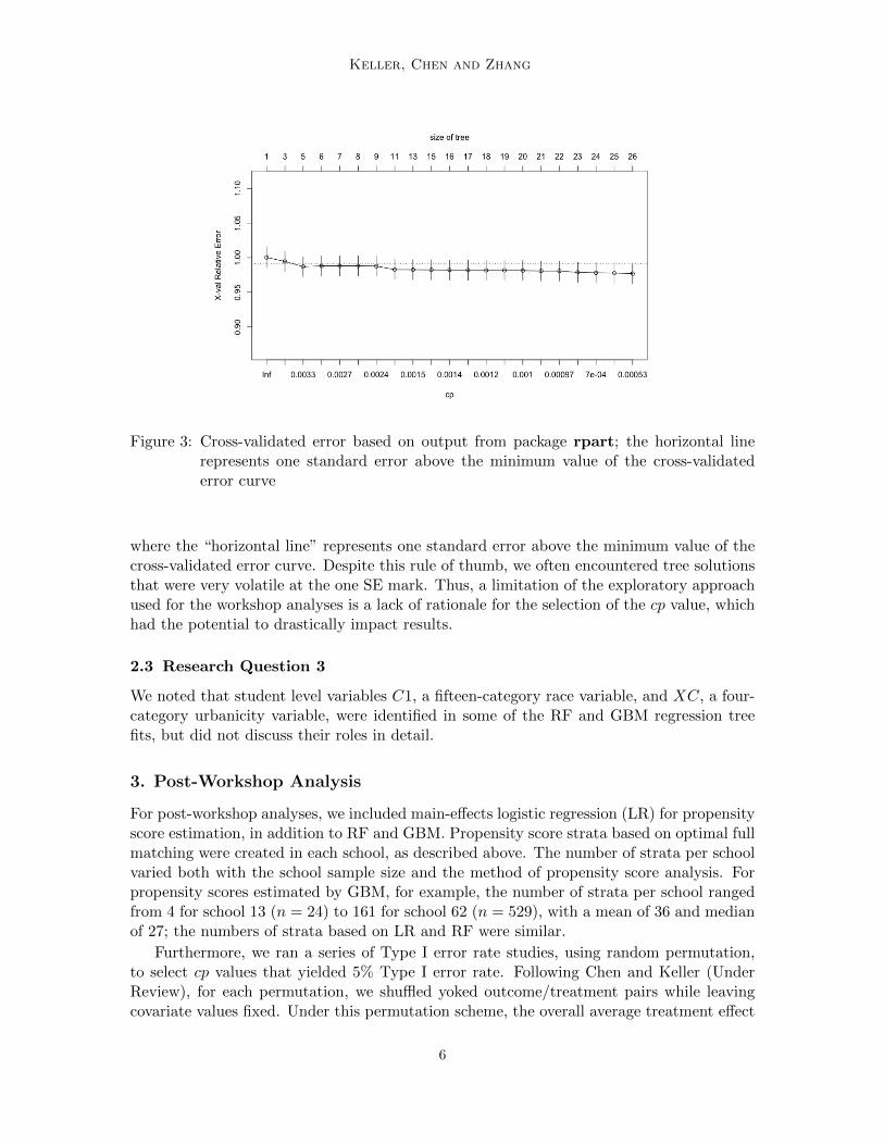
Although we did examine the results of ten-fold cross-validation for cp produced bythe rpart package, we encountered multiple situations in which the cross-validated errorrate continued to decrease without bound as the value of the tuning parameter decreased(i.e., favoring more and more complex tree structures; see Figure 3 for an example). Theadvice given in the rpart manual (Therneau et al., 2015) is that “A good choice of cpfor pruning is often the leftmost value for which the mean lies below the horizontal line.”

5


Figure 3: Cross-validated error based on output from package rpart; the horizontal linerepresents one standard error above the minimum value of the cross-validatederror curve

where the “horizontal line” represents one standard error above the minimum value of thecross-validated error curve. Despite this rule of thumb, we often encountered tree solutionsthat were very volatile at the one SE mark. Thus, a limitation of the exploratory approachused for the workshop analyses is a lack of rationale for the selection of the cp value, whichhad the potential to drastically impact results.


We noted that student level variables C1, a fifteen-category race variable, and XC, a four-category urbanicity variable, were identified in some of the RF and GBM regression treefits, but did not discuss their roles in detail.

3. Post-Workshop Analysis

For post-workshop analyses, we included main-effects logistic regression (LR) for propensityscore estimation, in addition to RF and GBM. Propensity score strata based on optimal fullmatching were created in each school, as described above. The number of strata per schoolvaried both with the school sample size and the method of propensity score analysis. Forpropensity scores estimated by GBM, for example, the number of strata per school rangedfrom 4 for school 13 (n = 24) to 161 for school 62 (n = 529), with a mean of 36 and medianof 27; the numbers of strata based on LR and RF were similar.

Furthermore, we ran a series of Type I error rate studies, using random permutation,to select cp values that yielded 5% Type I error rate. Following Chen and Keller (UnderReview), for each permutation, we shuffled yoked outcome/treatment pairs while leavingcovariate values fixed. Under this permutation scheme, the overall average treatment effect

6


and the covariate marginal distributions and interrelationships remain unperturbed; mean-while, any dependence between covariates and individual treatment effects is destroyed,which provides recourse to the permutation null hypothesis of no effect (Rubin, 1980; Keller,2012).

For research questions 2 and 3 for the post-workshop analyses we distinguish betweentesting and exploration. We test for effect heterogeneity by using cp values that werefound, through permutation, to hold the rate of false positives to the nominal 5% level;results based on these cp values are appropriate for inferential decision-making. We explore(a) graphically, by examining graphical depictions of key relationships, and (b) quanti-tatively, by ranking variable importance ratings from random forest fits. Although theseexplorations are suitable for hypothesis generation for future study, they are not appropriatefor inferential decision-making.


We found that the desired nominal Type I error rate of approximately 5% was attained forGBM, RF, and LR, respectively, for cp values of 0.006 0.008, and 0.006. The overall ATEestimates were hardly changed when using the cp values determined through permutation.For propensity score estimation via GBM, RF, and LR, respectively, the overall ATE es-timates, with 95% nonparametric bootstrap confidence intervals (percentile method), were0.25 (0.22, 0.30), 0.26 (0.22, 0.30), and 0.27 (0.24, 0.28).

3.2 Research Questions 2 & 3

3.2.1 Testing

For propensity scores estimated via LR, and with cp = 0.006, one split on variable XC = 3was flagged. No splits were identified using propensity scores estimated via RF with cp =0.008, nor via GBM with cp = 0.006. Thus, we found some evidence of effect heterogeneitybased on XC, but the finding was not robust to propensity score specification. There wasno evidence of significant effect heterogeneity for any other covariates.

3.2.2 Exploration

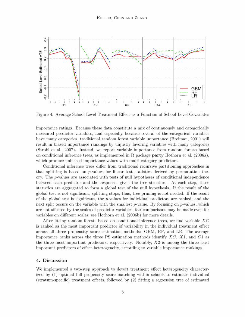
In Figure 4 we plot nonparametric regression curves to show the relationship between school-level estimates of the average treatment effect on the vertical axis against each school-levelcovariate. The notion that the intervention was more effective for schools in a “middlerange” on X2 and with lower values on X1 is not inconsistent with the relationships shownin the first two panels of Figure 4.

In Figure 5, because the student-level covariates are categorical, we use conditionalboxplots to show how individual treatment effect estimates vary by category across thefive student-level covariates. We note what appears to be considerable variability in bothmedian and interquartile range across levels of C1, the 15-category race variable. We alsonote a lower median for category XC = 3 as compared with the other categories of XC, afive-category urbanicity variable.

Finally, we fit random forests using the vector of individual treatment effect estimatesas outcome and the school- and student-level variables as predictors to calculate variable

7


Figure 4: Average School-Level Treatment Effect as a Function of School-Level Covariates

importance ratings. Because these data constitute a mix of continuously and categoricallymeasured predictor variables, and especially because several of the categorical variableshave many categories, traditional random forest variable importance (Breiman, 2001) willresult in biased importance rankings by unjustly favoring variables with many categories(Strobl et al., 2007). Instead, we report variable importance from random forests basedon conditional inference trees, as implemented in R package party Hothorn et al. (2006a),which produce unbiased importance values with multi-category predictors.

Conditional inference trees differ from traditional recursive partitioning approaches inthat splitting is based on p-values for linear test statistics derived by permutation the-ory. The p-values are associated with tests of null hypotheses of conditional independencebetween each predictor and the response, given the tree structure. At each step, thesestatistics are aggregated to form a global test of the null hypothesis. If the result of theglobal test is not significant, splitting stops; thus, tree pruning is not needed. If the resultof the global test is significant, the p-values for individual predictors are ranked, and thenext split occurs on the variable with the smallest p-value. By focusing on p-values, whichare not affected by the scales of predictor variables, fair comparisons may be made even forvariables on different scales; see Hothorn et al. (2006b) for more details.

After fitting random forests based on conditional inference trees, we find variable XCis ranked as the most important predictor of variability in the individual treatment effectacross all three propensity score estimation methods: GBM, RF, and LR. The averageimportance ranks across the three PS estimation methods identify XC, X1, and C1 asthe three most important predictors, respectively. Notably, X2 is among the three leastimportant predictors of effect heterogeneity, according to variable importance rankings.

4. Discussion

We implemented a two-step approach to detect treatment effect heterogeneity character-ized by (1) optimal full propensity score matching within schools to estimate individual(stratum-specific) treatment effects, followed by (2) fitting a regression tree of estimated

8


Figure 5: Individual Treatment Effect as a Function of Student-Level Predictors by Propen-sity Score Estimation Method; GBM = Generalized Boosted Modeling, RF =Random Forests, LR = Logistic Regression

Figure 6: Variable Importance Rankings from Random Forest Runs Regressing the Indi-vidual Treatment Effect Estimates on the Ten Predictors of Interest

9


individual treatment effects on covariates. In the analyses prepared for the workshop, wefocused on the second research question by exploring the relationships between X1, X2,and estimated school-level treatment effects. For the post-workshop analyses, we furtherdemarcated analyses by distinguishing between testing and exploration.

In general, our analyses leaned heavily on the regression tree algorithm, which was used(a) in estimating propensity scores via random forests and boosted modeling, (b) to test foreffect heterogeneity through regression tree analysis of individual treatment effect estimates,and (c) for additional exploration through conditional random forest variable importance.With respect to fitting regression trees, we noted that ten-fold cross-validation and theone SE rule of thumb, both methods typically used to select the cost complexity pruningparameter, cp, are inconclusive with respect to Type I error rate. Instead, we used a simplepermutation approach to select cp values that yielded the desired Type I error rate andenabled testing.

For the first research question, we found that the average intervention effect estimates bydifferent methods were all positive, with 95% bootstrap confidence intervals indicating thatthe mindset intervention was effective in improving student achievement. For the second andthird research questions, we found evidence of heterogeneity based on membership in thethird category of the urbanicity variable, but the finding was not robust to propensity scoreestimation method. We found no other significant evidence of treatment effect modification.Based on exploratory analyses, if we were to plan a follow-up study to search for effectmodification, we would recommend focusing on the student-level urbanicity variable, XC,the student level race variable, C1, and the school-level fixed mindset rating variable, X1.We would not recommend prioritizing X2, the school-level achievement variable.

As noted by Feller and Holmes (2009), the assumptions required for identification ofCATEs are identical to those required for the overall ATE (i.e., strong ignorability, nointerference between units, single version of each treatment). We assume these key as-sumptions are met here. Furthermore, the usual recommended steps for the specificationof the propensity score, including iterative respecification to achieve acceptable balanceon observed covariates and an examination of overlap are also important, but details areomitted because our focus is on heterogeneous subgroup identification. Finally, resamplingapproaches such as the jackknife, bootstrap, and boosting may be used to attain errorbounds on ATEs and CATEs estimated via our two-step approach; however, care must betaken when using resampling techniques to estimate standard errors for estimators thatinvolve matching (Abadie and Imbens, 2008; Austin and Small, 2014).

Acknowledgments

We thank Carlos Carvalho, Avi Feller, Jennifer Hill, and Jared Murray for organizing theworkshop and inviting our submission. Jianshen Chen was employed by Educational TestingService when this work was carried out.

10


References

A. Abadie and G. W. Imbens. On the failure of the bootstrap for matching estimators.Econometrica, 76:1537–1557, 2008.

P. C. Austin and D. S. Small. The use of bootstrapping when using propensity-scorematching without replacement: a simulation study. Statistics in Medicine, 33:4306–4319,2014.

L. Breiman. Random forests. Machine Learning, 45:5–32, 2001.

L. Breiman, J. H. Friedman, R. A. Olshen, and C. J. Stone. Classification and RegressionTrees. Wadsworth and Brooks/Cole, Monterey, CA, 1984.

J. Chen and B. Keller. Heterogeneous subgroup identification in observational studies.Manuscript submitted for publication, Under Review.

A. Feller and C. Holmes. Beyond toplines: Heterogeneous treatment effects in randomizedexperiments. Technical report, University of Oxford, July 2009.

Torsten Hothorn, Peter Buehlmann, Sandrine Dudoit, Annette Molinaro, and Mark VanDer Laan. Survival ensembles. Biostatistics, 7(3):355–373, 2006a.

Torsten Hothorn, Kurt Hornik, and Achim Zeileis. Unbiased recursive partitioning: Aconditional inference framework. Journal of Computational and Graphical Statistics, 15:651–674, 2006b.

B. Keller. Detecting treatment effects with small samples: The power of some tests underthe randomization model. Psychometrika, 77:324–338, 2012.

Mindset Scholars Network. National study of learning mindsets. 2018. URLhttp://mindsetscholarsnetwork.org.

J. Neyman. Sur les applications de la theorie des probabilites aux experiences agricoles:Essai des principes. In Roczniki Nauk Rolniczych, volume X, pages 1–51. In Polish, Englishtranslation by D. Dabrowska and T. Speed in Statistical Science 5, 465 - 72, 1990., 1923.

R Core Team. R: A language and environment for statistical computing. 2018. URLhttp://www.R-project.org/.

P. R. Rosenbaum and D. B. Rubin. The central role of the propensity score in observationalstudies for causal effects. Biometrika, 70:41–55, 1983.

D. B Rubin. Estimating causal effects of treatments in randomized and nonrandomizedstudies. Journal of Educational Psychology, 66:688–701, 1974.

D. B. Rubin. Randomization analysis of experimental data: The Fisher randomization testcomment. Journal of the American Statistical Association, 75:591–593, 1980.

P. M. Steiner, T. D. Cook, and W. R. Shadish. On the importance of reliable covariate mea-surement in selection bias adjustments using propensity scores. Journal of Educationaland Behavioral Statistics, pages 213–236, 2011.

11


C. Strobl, A.–L. Boulesteix, A. Zeileis, and T. Hothorn. Bias in random forest variableimportance measures: Illustrations, sources and a solution. BMC Bioinformatics, page8:25, 2007.

T. Therneau, B. Atkinson, and B. Ripley. rpart: Recursive partitioning and regression trees.R package version 4.1-9, 2015. URL http://CRAN.R-project.org/package=rpart.

12

keller chen zhang forthcoming - columbia university

Documents