keynote presentation by prof. david r. fox envirotox ... address.pdf · keynote presentation by...
TRANSCRIPT
Statistics and Ecotoxicology: Past, Present and Future
Keynote Presentation
by
Prof. David R. Fox
EnviroTox, Darwin 18 April 2011

1
2
Introduction
Good morning. It is indeed an honour and privilege to be invited to talk at
Envirotox 2011 which is jointly sponsored by the Australasian Society for
Ecotoxicology, the Royal Australian Chemical Institute, and SETAC Australasia. I am
particularly indebted to conference co-chairs Michelle Iles and Rick van Dam for
extending me this invitation and for their months of hard work in bringing this
conference to fruition. I also wish to acknowledge the traditional landowners, the
Larrakia Aboriginal people.
As a statistician I understand the concept of an „outlier‟. According to Wolfram
Research, “an outlier is an observation that lies outside the overall pattern of a
distribution. Usually, the presence of an outlier indicates some sort of problem”. I
sincerely hope that my participation in this conference for ectoxicologists is not
viewed as indicating some sort of problem! To the contrary – I have an almost
evangelical zeal about the potential for statistics to contribute and potentially make a
difference to the theory and practice of modern-day ecotoxicology.
My interest in the statistical aspects of ecotoxicology dates back to the mid-
1990s when I was working in
CSIRO – firstly as a
statistician on the Port Phillip
Bay Environmental Study and
then as Director of the
Effluent Management Study
which was undertaken on
behalf of Melbourne Water. I
remember listening to many
study updates at our regular meetings of the scientific committee and being
particularly impressed and interested in the work of
Jenny Stauber, Graeme Batley and others who with
CSI-like skills, committed themselves to the task of
solving the particularly heinous crime of „Hormosira
homicide‟ down at a lonely beach called Boags
Rocks – some 15 km to the south-east of the site of

3
the infamous disappearance of another
species H. Holtii. As it turns out, the
fate of a prime minister dressed in
rubber in the presence of three scantily
clad females was a harder case to
crack than the identification of the toxic
agent for Hormosoria.
However, I digress. Let me
return to my thesis which is: the union
of statistics and (eco)toxicology is
deserving of formal recognition. Last
year I published a Learned Discourse in IEAM having the somewhat rhetorical title of
“Statistics and Ecotoxciology: Shotgun Marriage or Enduring Partnership?‟
In this short presentation I wish to establish
the credentials of the bride and groom in
this scientific partnership and propose that
the parents resist the temptation of a US-
style „quickie‟ marriage and instead commit
to a celebration more befitting of this most
worthwhile enterprise.

4
On its website, your society, the ASE acknowledges the multidisciplinary
nature of the endeavour. Specifically, it says “the field of ecotoxicology includes
concepts arising from disciplines such as toxicology, biology, analytical,
environmental and organic chemistry, physiology, ecology, genetics, microbiology,
biochemistry, immunology, molecular biology, soil, water and air sciences, and
economics”. Curious - no mention of statistics? Perhaps we can have that changed?
Yesterday was the 17th. anniversary of the death
of Roger Wolcott Sperry. Sperry was an American
neurobiologist who shared the 1981 Nobel Prize in
Medicine for revolutionising our understanding of brain
function. Sperry and his colleagues identified the unique
capabilities of each hemisphere and demonstrated that
the combined effect of bi-hemispheric activity amounted
to more than the simple additive effects of the two
separate hemispheres. A primal
case of a biological synergism that
we all rely on - or at least most of us rely on!
Like the brain, ecotoxicology relies on different
„hemispheres‟ of knowledge, expertise, and wisdom to
operate effectively, make informed decisions, and to react
decisively. In this depiction I see the newlyweds working
together, standing on the bridge that links the disciplines,
roadmap in hand and a clear sense of direction.

5
In the remainder of this talk I
want to commence by providing an
historical sketch of the separate
paths of statistics and ecotoxicology;
highlighting the intersections of our
disciplines and the successes we‟ve
enjoyed along the way. I will then
briefly touch on what I consider to be
some unresolved ecotoxicological
issues that will only be solved by
strengthening existing „hemispherical
linkages‟ and developing new ones.
Finally, I will conclude with some remarks on what I perceive to be challenges for the
future.
The genealogical tree
It is probably true to say that humans became conscious of their own mortality
shortly after climbing out of the trees. Like all animals, we would have quickly learnt
from trial-and-error „experiments‟ what was safe for us to eat and drink and what was
not. When we actually codified this knowledge is not entirely clear although the
works of Pendanius Dioscorides and others certainly establishes that this activity
was well underway almost 2,000 years ago.
Dioscorides was a Greek physician,
pharmacologist, botanist and author of a five volume
encyclopaedia about herbal medicines called „De
Materia Medica‟ that is the pre-cursor to modern
pharmacopeias. Some 1400 years later, Paracelsus
declared that “all substances are poisons; there is
none which is not a poison. The right dose
differentiates a poison from a remedy”.
Statistics (Eco)Toxicology
J. Theodore
Cash
J. W. TrevanJ. Berkson

6
The De Materia Medica was circulated in
Latin, Greek and Arabic. One of the most
important was the illustrated Greek version
„Vienna Dioscorides‟ which was discovered in
Istanbul in the 1560s.
So let us now time-travel at warp-factor 3
to the industrio-chemical revolution of the mid-
19th. century. Now, for the first time we have
releases of new chemicals and substances
hitherto
never seen before. Shortly thereafter,
scientists began conducting the very first
toxicity studies in the 1900s and, importantly
we see the first use of „toxicity.
In 1908, Theodore Cash published a paper in the British Medical Journal, in
which he described early dose-response experiments. In his paper he talks of “the
7
nearest fulfilment of a mathematical relationship seemed to be achieved by working
upwards from that amount of any drug which produced the minimum of appreciable
action”. This dose, he notes was variously referred to as the “Grenzdose” or “limit
dose”. I find this companion development of toxicological nomenclature and
acronyms fascinating and something which has survived, if not thrived over the last
100 years. While we now have NOECs, NECs, ECxs, NOAELs, LOECS, LDxs, ICxs
etc., back in 1908 Cash was making early inroads with the introduction of the
additional terms “minimal effective dose” and “maximal ineffective dose”.
While these early scientific studies were important in establishing safe doses
for medicines they had little immediate application to the more diffuse area of
chemicals in the environment. Another ½ century would have to pass
before the emergence of the environmental movement. An important
development along the way was the establishment in the United States of
the FDA in 1930 and the passing of the Food, Drug, and Cosmetics Act
in 1938.
Things were about to get a lot tougher for the burgeoning chemical industry.
In 1958 an amendment to the Act known as the Delaney Clause prohibited the
approval of any food additive shown to cause cancer in humans or animals.
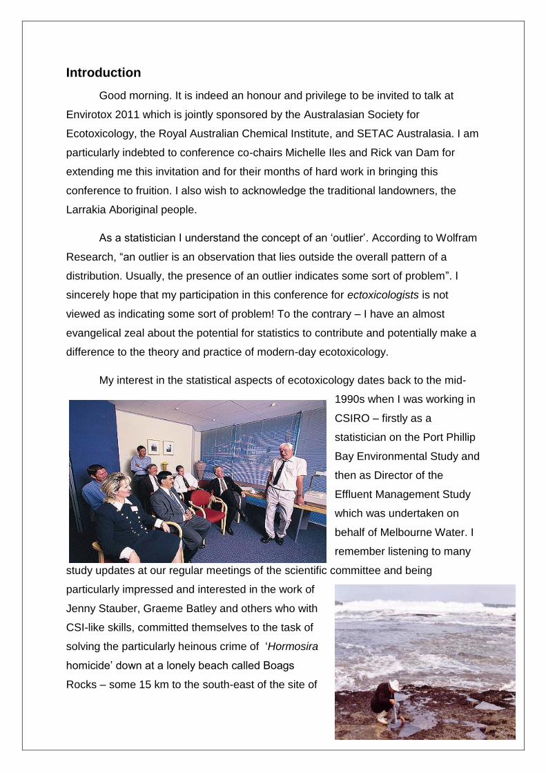
In 1962 American marine biologist and
conservationist, Rachel Carson released “Silent
Spring”. This was a turning point, the epiphany that
awakened the world to the possibility that
chemicals (particularly pesticides such as DDT) in
the environment were having both human and
ecological impacts. The decade between 1965 and
1975 saw a flurry of intense scientific investigations
into the acute and chronic effects of pollutants on
aquatic organisms. The results of these studies
reduced some of the uncertainty associated with
the application of arbitrary „safety‟ or „assessment‟ factors derived from human
toxicity studies but, as we shall see, introduced other difficulties with statistical
estimation and inference.

8
The 1970s commenced with the introduction of the word
ecotoxicology by Rene Truhaut and this decade was to be
characterised by research into whole organism responses and
effects in biological systems.
The journal Aquatic Toxicology was
launched in 1981 in response to what it claimed was a world-wide
concern about the effects of man-made chemicals on aquatic
organisms and ecosystems. Today we see no fewer than 20 sub-
disciplines of toxicity although interestingly none concerning the statistical aspects of
toxicology and/or ecotoxicology.
The last thirty years has been witness to ever-increasing mathematical and
statistical sophistication of the treatment of data and modelling approaches used in
ecotoxicology. However, there are still „burrs under the saddle‟ – the problematic
NOEC; the legitimacy of using mixtures of toxicity measures in SSD modelling; SSD
modelling itself and the whole statistical underpinning of the method; Bayesian
versus Frequentist statistical paradigms; „time‟ as the missing dimension in
concentration-response modelling; and individual versus population effects to name
a few.
I now wish to „shift gears‟ and trace the development of what I call statistical
ecotoxicology.
9
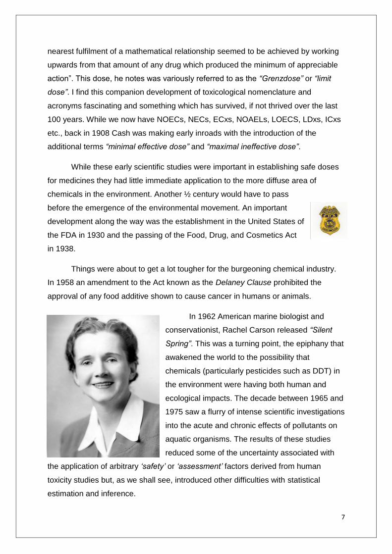
The role of statistics in Ecotoxicology
We only need look at this page from Posthuma et
al or the flowchart for the Fathead Minnow larval
survival and growth test to see that statistical
methods play a critical role in the assessment of
toxicity. Following the flowchart logic, our
immediate choice is to either undertake a probit
analysis of the survival data or to transform it
using the arcsine transformation. The
transformed data (which interestingly are now in
units of angular radians) are then to be checked
for their distributional normality using the
Shapiro-Wilks test. Should they pass this test,
these angles are checked for homogeneity of
variance using Bartlett‟s test. A satisfactory
result on this test allows us to proceed to the
ubiquitous Dunnett‟s test if we have equal
numbers of replicates or, in the case of
unequal replicates – the rather formidable-
sounding T-test with Bonferroni adjustment.
Over on the other side of the flow chart, we are
led to either Steel‟s many-to-one rank test or
the Wilcoxon rank sum test with Bonferroni
adjustment.

10
So, how did ecotoxicology become so heavily dependent on statistics?
To answer this, we need to go back to the late 60s / early 70s when, in April 1968 a
small group of people concerned about the future of humankind met in Rome. The
Club of Rome as it became known commissioned a report into the sustainability of
economic growth and the ensuing report
„Limits to Growth‟ was published in 1972.
The „Limits to Growth‟ made predictions
using fairly simplistic mathematical
models of population growth and resource
availability. For us, the important
connection is the similarity of these
models with the Malthusian growth model
– named after the British scholar, Rev. Thomas Malthus who,
some 175 years earlier had realised that population growth
could not be limitless. The first important link between
statistical science and the environmental movement has now
been established for the Malthusian growth model is a direct
ancestor of the logistic function which was published
(posthumously) in 1858 by Francois Verhulst. We will return
to the logistic function shortly, but let us continue following the
statistical footprint.
Verhulst was a Belgium mathematician. His interest in
population modelling commenced while he was at the
University of Ghent studying under Adolphe
Quetelet. Quetelet was an astronomer,
mathematician, statistician, and sociologist and
was the first to apply the normal distribution to
sociological phenomena. He also gave us the
Quetlet Index of obesity which we recognise
today as the BMI.
Like Malthus, Quetelet was also aware of the limitations of simple exponential
growth models and asked Verhulst to look at the problem with a view to modifying

11
the model so as to provide more realistic population estimates as t→∞.
Verhulst succeeded in this task and published an equation relating population size to
intrinsic growth rate and carrying capacity – he referred to his solution as the logistic
function or logistic equation.
For some unknown reason the logistic equation remained a relatively obscure
mathematical result until it was rediscovered in 1920 by Raymond Pearl and Lowell
Reed.
Pearl had just been appointed director of the
department of Biometry and Vital Statistics at John Hopkins
University and Reed was his deputy. Although a biologist by
training, Pearl was deeply interested in
statistics and had in fact spent a year
in 1905-06 in London with eminent
statistician Karl Pearson (one of the
pioneers of modern hypothesis
testing). Pearl and Reed were, at the
time, unaware of Verhulst‟s work and had independently
derived the logistic equation themselves.
While Pearl and Reed were not mainstream statisticians,
Udny Yule certainly was. In his 1925 Presidential address to the
Royal Statistical Society, Yule commented on Pearl and Reed‟s
independent discovery of Verhulst‟s result and cemented the term
“logistic” in the statistical lexicon when he remarked that “I have
relegated to Appendix II some discussion of the mathematics of
the curve, which, following Verhulst, we may term a „logistic‟”.
Now the link with toxicology. Two years after Yule‟s Presidential address to
the Royal Statistical Society, English physiologist J.W. Trevan gave a paper to the
Royal Society in London in which he wanted to establish “a more accurate definition
of such terms as „minimal lethal dose‟, minimal effective dose‟ etc.” Trevan
suggested that the term „minimum lethal dose‟ be dropped altogether and that
12
toxicity should be stated primarily in terms of the median lethal dose which he
abbreviated as LD50.
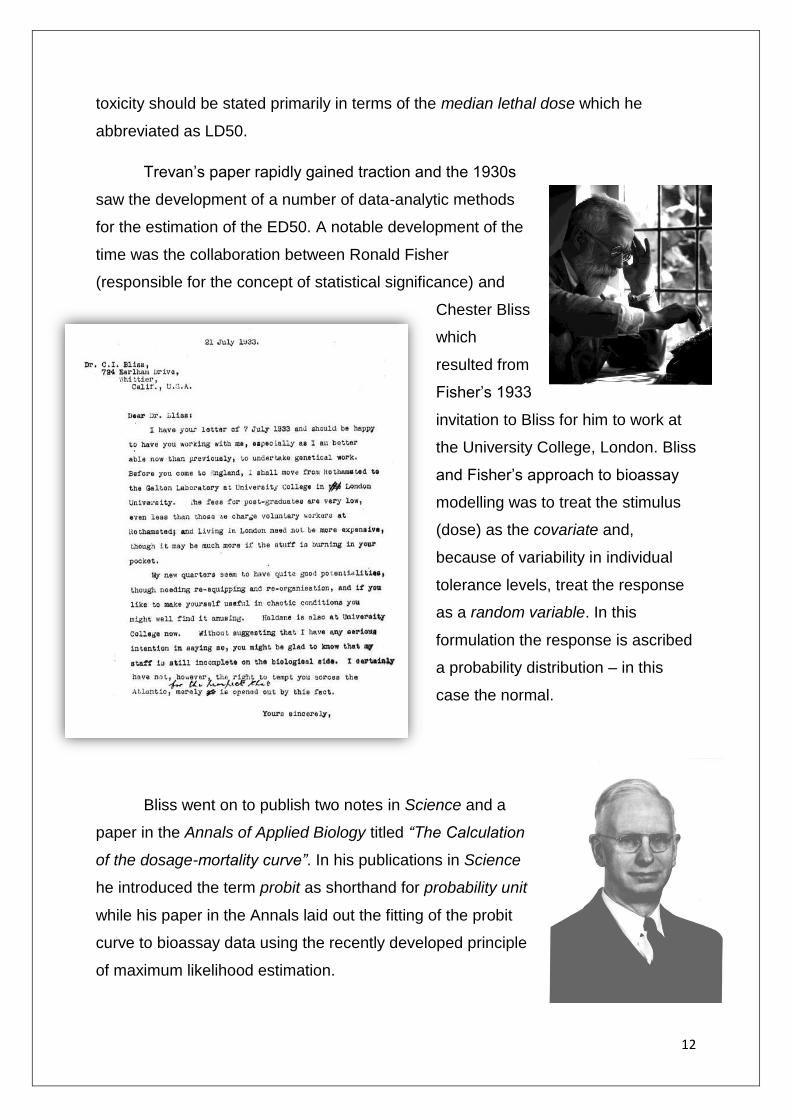
Trevan‟s paper rapidly gained traction and the 1930s
saw the development of a number of data-analytic methods
for the estimation of the ED50. A notable development of the
time was the collaboration between Ronald Fisher
(responsible for the concept of statistical significance) and
Chester Bliss
which
resulted from
Fisher‟s 1933
invitation to Bliss for him to work at
the University College, London. Bliss
and Fisher‟s approach to bioassay
modelling was to treat the stimulus
(dose) as the covariate and,
because of variability in individual
tolerance levels, treat the response
as a random variable. In this
formulation the response is ascribed
a probability distribution – in this
case the normal.
Bliss went on to publish two notes in Science and a
paper in the Annals of Applied Biology titled “The Calculation
of the dosage-mortality curve”. In his publications in Science
he introduced the term probit as shorthand for probability unit
while his paper in the Annals laid out the fitting of the probit
curve to bioassay data using the recently developed principle
of maximum likelihood estimation.
13
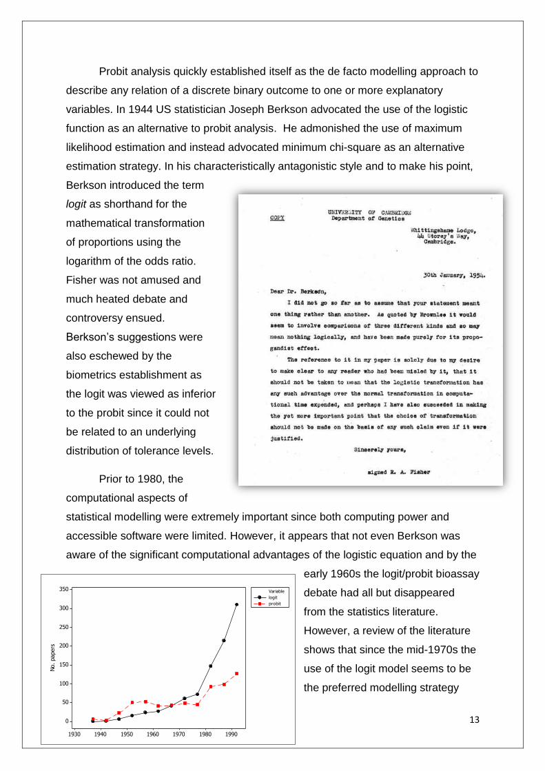
Probit analysis quickly established itself as the de facto modelling approach to
describe any relation of a discrete binary outcome to one or more explanatory
variables. In 1944 US statistician Joseph Berkson advocated the use of the logistic
function as an alternative to probit analysis. He admonished the use of maximum
likelihood estimation and instead advocated minimum chi-square as an alternative
estimation strategy. In his characteristically antagonistic style and to make his point,
Berkson introduced the term
logit as shorthand for the
mathematical transformation
of proportions using the
logarithm of the odds ratio.
Fisher was not amused and
much heated debate and
controversy ensued.
Berkson‟s suggestions were
also eschewed by the
biometrics establishment as
the logit was viewed as inferior
to the probit since it could not
be related to an underlying
distribution of tolerance levels.
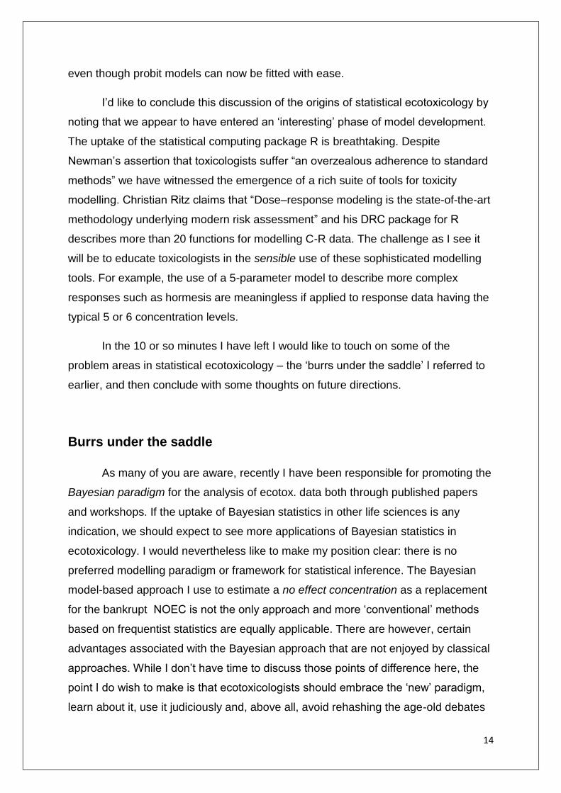
Prior to 1980, the
computational aspects of
statistical modelling were extremely important since both computing power and
accessible software were limited. However, it appears that not even Berkson was
aware of the significant computational advantages of the logistic equation and by the
early 1960s the logit/probit bioassay
debate had all but disappeared
from the statistics literature.
However, a review of the literature
shows that since the mid-1970s the
use of the logit model seems to be
the preferred modelling strategy
1990198019701960195019401930
350
300
250
200
150
100
50
0
No. papers
logit
probit
Variable
14
even though probit models can now be fitted with ease.
I‟d like to conclude this discussion of the origins of statistical ecotoxicology by
noting that we appear to have entered an „interesting‟ phase of model development.
The uptake of the statistical computing package R is breathtaking. Despite
Newman‟s assertion that toxicologists suffer “an overzealous adherence to standard
methods” we have witnessed the emergence of a rich suite of tools for toxicity
modelling. Christian Ritz claims that “Dose–response modeling is the state-of-the-art
methodology underlying modern risk assessment” and his DRC package for R
describes more than 20 functions for modelling C-R data. The challenge as I see it
will be to educate toxicologists in the sensible use of these sophisticated modelling
tools. For example, the use of a 5-parameter model to describe more complex
responses such as hormesis are meaningless if applied to response data having the
typical 5 or 6 concentration levels.
In the 10 or so minutes I have left I would like to touch on some of the
problem areas in statistical ecotoxicology – the „burrs under the saddle‟ I referred to
earlier, and then conclude with some thoughts on future directions.
Burrs under the saddle
As many of you are aware, recently I have been responsible for promoting the
Bayesian paradigm for the analysis of ecotox. data both through published papers
and workshops. If the uptake of Bayesian statistics in other life sciences is any
indication, we should expect to see more applications of Bayesian statistics in
ecotoxicology. I would nevertheless like to make my position clear: there is no
preferred modelling paradigm or framework for statistical inference. The Bayesian
model-based approach I use to estimate a no effect concentration as a replacement
for the bankrupt NOEC is not the only approach and more „conventional‟ methods
based on frequentist statistics are equally applicable. There are however, certain
advantages associated with the Bayesian approach that are not enjoyed by classical
approaches. While I don‟t have time to discuss those points of difference here, the
point I do wish to make is that ecotoxicologists should embrace the „new‟ paradigm,
learn about it, use it judiciously and, above all, avoid rehashing the age-old debates

15
about the legitimacy of subjective probabilities or the arbitrariness of picking a
suitable prior probability density. I have been challenged on this latter point by
ecotoxicologists who eschew the notion of a subjective prior yet seem to ignore the
inconvenient truth that the blind faith they entrust to the results from ToxCalc is
underpinned on a (not insignificant) number of assumptions and somewhat arbitrary
modelling choices.
The traditional approach to statistical modelling is illustrated in this slide.
Data and a model are brought together to estimate parameters. We use a statistical
test or suite of tests to assess the adequacy of the fit. The model may require
refinement and/or additional data to be collected. We cycle through this process to
develop a parsimonious description of the response-generating mechanism. We
summarise the results and then stop.
The situation in ecotoxicology is a little different – the systems we are
Data
Model
Fit model SummariseAdequate
fit?
No
Stop
Yes
Adapted from Nelder, 1999
New data
What process?
Update existing model or
start again?
What model?

16
describing are invariably dynamic and with the passage of time comes additional
data and new insights.
We might repeat the modelling process, but some decisions have to be made
about the form of the model and the method of updating our toxicity estimates,
triggers, „safe‟ concentrations etc.
Other „difficulties‟ requiring closer attention are:
1. The design of C-R experiments. I‟m not talking of the analytical lab.
methods – they‟re well defined. What is less well defined is a
contemporary „roadmap‟ to assist in making decisions about the
number and spacing of concentrations to use; how much replication is
required; how to choose a plausible mathematical model – or at the
very least, how to eliminate unsuitable ones; how to estimate model
parameters and associated uncertainty; how and when to transform
data; when or if toxicity measures should be pooled; characterisations
of the SSD; and so on.
To be fair, there are a number of statistical guides for ecotoxicology such as those
published by Environment Canada and the OECD and Australia and New Zealand
are presently working on their own. However, some of this information – particularly
in the Canadian document – is so out-dated, and dare I say, flawed, as to render the
advice next to useless. This may seem unfairly harsh, however by way of example,
the blanket requirement of the Canadian “Guidance Document on Statistical
Methods for Environmental Toxicity Tests” to always use log-transformed data is
both perplexing and unwarranted. Furthermore, the claim that “Canadian
investigators …are often reluctant and sometimes actively hostile to the idea of
continuing with logarithms for statistical analysis” because, it is suggested, Canadian
scientists and technicians have a lack of familiarity with the complexity of logarithms
is disingenuous and, frankly insulting. Other advice such as estimating an EC50 from
a hand-drawn graph and fitting probit curves by eye is nothing short of astonishing.
Even Chester Bliss and Ronald Fisher had better algorithms for doing this before the
first computer was even invented! But then again, the Canadian document refers to

17
the existence of “modern computers” as an alternative to hand-calculation and
furthermore recommends the use of a software tool developed in 1978 and modified
for the Windows operating system in 1995! Hardly contemporary stuff!
2. Challenging the assumptions. Contemporary approaches to the
identification of a „safe‟ concentration or dilution of some contaminant
rely on a plethora of statistical approaches – from simple (or if you‟re
Canadian, very difficult) arcsine and logarithmic transformations of the
raw toxicity data to advanced tools for mathematical modelling and
statistical inference. We know the NOEC is flawed, but struggle to find
suitable alternatives. A common practice, driven by data paucity or
claims of superiority, is to use various combinations of NOECs, ECxs,
ICxs, or arbitrarily scaled versions of these as inputs into the SSD
modelling stage where again we make somewhat arbitrary decisions
about the distributional form of the SSD and the data
inclusion/exclusion rules. Rather than undertaking more investigations
to characterise the difference between say a lognormal SSD and a log-
logistic SSD what I believe we need are some well-designed
experiments to test the claims that some high fraction of all species is
protected provided the environmental concentration of a contaminant is
below the threshold or trigger value. Standard C-R test procedures
could also benefit from an assessment of the effects of ignoring the
time dimension and the consequences of a less than comprehensive
assessment of variability. These are the topics of two talks in the
Environmetrics session after morning tea.
3. Being clear on what we‟re doing. If, as I‟ve suggested, we move more
to model-based inference for deriving toxicity measures, then it is
incumbent upon us to use credible models. For any modeller, the truth
is expressed by the fact that data = model + error. Thus our
representation of what we observe has two components: a
deterministic component and a stochastic component. The ready
accessibility of programs like ToxCalc sometimes means that we spend

18
either no time or too little time thinking about suitable structures for
these model components. ToxCalc provides toxicity estimates that are
both empirical (such as a NOEC) and model-based (such as an EC10)
although the choices are limited, automated, and not readily apparent.
Indeed, one of the selling points boasted on Tidepool‟s web site
is that ToxCalc “automatically chooses the appropriate methods and
data transforms”. What is not well understood is that programs like
ToxCalc base their statistical inference (eg. confidence intervals) on
the assumption that the error term follows a normal probability model.
Part of ToxCalc‟s automation is the use of mathematical
transformations to beat the data into some semblance of normality
when those data fail a test of normality. A more discerning modeller
would think about an appropriate error structure for the data at hand.
For example, toxicologists commonly deal with survival data of the form
“r animals surviving out of n”.
For example, here we see data relating the number of fish out of an
initial five surviving at various times as a function of effluent
concentration.
n(x)=5 r(x)
x
43210
0.5
0.4
0.3
0.2
0.1
0.0
X
Pro
ba
bili
ty
Distribution PlotBinomial, n=5, p=0.14375
543210-1-2-3-4
0.30
0.25
0.20
0.15
0.10
0.05
0.00
X
De
nsit
y
Distribution PlotNormal, Mean=0.71875, StDev=1.30098

19
One only needs to think about this for a nanosecond to realise that the
response variable (r) is discrete whereas the normal distribution is a
continuous probability model. Not to worry, you recall your crusty old
statistics professor mumbling something about the law of large
numbers or the central limit theorem as the universal life buoy in such
cases of disconnect and happily proceed without giving it any further
thought. Provided n is „large‟ (and the statistical version of „large‟ is
typically n>30) you won‟t drown. But what happens when n is small –
like 5? Well, in such cases the normal distribution will not provide much
buoyancy. A better strategy is to start with an error model that is both
commensurate with the scale of measurement and which is plausible.
The poisson, binomial and negative binomial probability models are
usually good candidates.
I will now finish with a few concluding remarks about challenges and opportunities.
Statistical Ectoxicology – Revitalising the marriage
In this short presentation I have attempted to highlight the
long, although not always visible, interaction between
statistics and ecotoxicology. One only needs thumb
through the pages of this text to appreciate the central
role of statistics in modern-day ecotoxicology.
I have used the metaphor of marriage to characterise the
relationship between our disciplines. On reflection –
perhaps it was a shotgun marriage. The „heady‟ days of
the 1960s and 70s witnessed a flurry of activity and
interaction that does not appear to have been sustained
into the new millennium. I can‟t be sure, but it seems like
cracks have developed which, if true, need to be
20
stemmed before they become chasms. The marriage needs rejuvenation - we need
a new roadmap and we need to reaffirm our vows.
So what does that mean exactly? Well, for me I‟d like to see a more enduring
engagement of statisticians with ecotoxicologists. Over the last 20 years we have
seen a de-skilling in quantitative capabilities in many agencies. Biometrics units and
the biometricians who worked in them are all but things of the past – casualties of
simple-minded economic policies that failed to understand that the benefits of good
statistical design and analysis far outweighed the cost of delivering such a service.
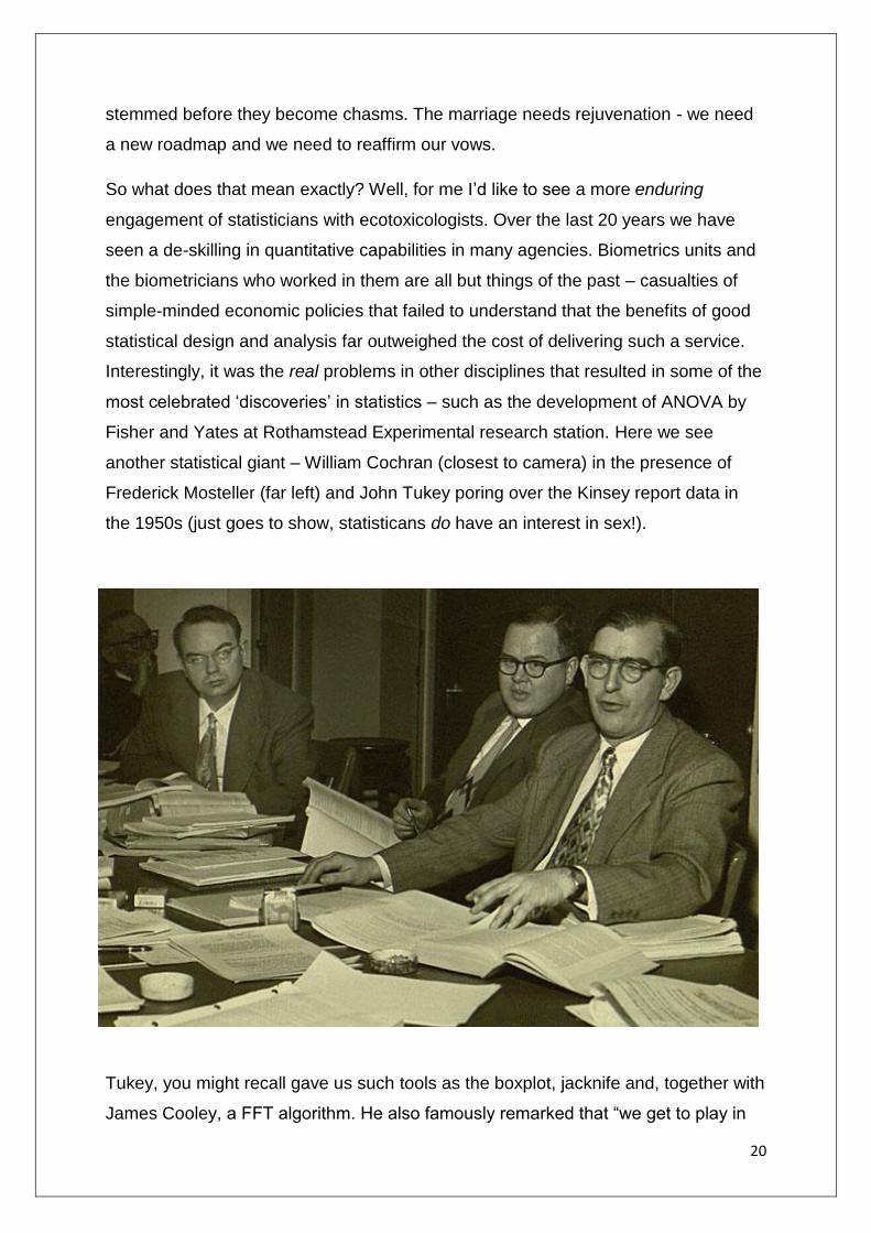
Interestingly, it was the real problems in other disciplines that resulted in some of the
most celebrated „discoveries‟ in statistics – such as the development of ANOVA by
Fisher and Yates at Rothamstead Experimental research station. Here we see
another statistical giant – William Cochran (closest to camera) in the presence of
Frederick Mosteller (far left) and John Tukey poring over the Kinsey report data in
the 1950s (just goes to show, statisticans do have an interest in sex!).
Tukey, you might recall gave us such tools as the boxplot, jacknife and, together with
James Cooley, a FFT algorithm. He also famously remarked that “we get to play in

21
everybody‟s backyard”. And that brings me to my point – statisticians are not playing
in your backyard! We have seen the profound impact of statisticians such as Fisher,
Bliss, and Berkson on quantitative developments in toxicology. But that was more
than 70 years ago. The 1980s and 90s saw a huge amount of work by quantitative
biologists and toxicologists into many aspects of SSD modelling but I struggle to
name a single statistician who has played a seminal role in these developments.
I will not dwell on the list of challenges for SSDs – Suter has done that already in
Chapter 21 of the text by Posthuma et al. Given the importance of the task, the
pervasiveness of the results, and the consequences of „getting it wrong‟, it is hard to
argue against a strengthening of quantitative skills in ecotoxicology. The path
already exists – we just have to take the first step. Thank you.