keywords: gasoline price, fuel economy, light duty...
TRANSCRIPT

Gasoline prices and fuel economy of new vehicles in Quebec
Keywords: gasoline price, fuel economy, light duty vehicles, feebate
Mots clefs: prix de l’essence, économie de carburant, véhicules légers, malus-bonus

1
Abstract We evaluate the short run impact of gasoline prices on new vehicles registrations by fuel economy using monthly data from 2002 to 2008 in the province of Quebec. We find that a gasoline price increase stimulates registration of new vehicles with a fuel consumption rate below 8.65L/100km (27.2 mpg) while it lowers those of vehicles above that limit. While the impact is modest for a large share of vehicles, we find that large gasoline price fluctuations can lead to noticeable changes in the composition of vehicles. The impact on the average fuel economy remains modest with an elasticity below -0.1. The federal feebate program had an impact of a 17% increase in sales of low-fuel consumption vehicles and a decrease of 8% of high-fuel consumption vehicles but the overall change in fuel economy was less than 1%.
Keywords: gasoline price, fuel economy, light duty vehicles, feebate

1
1. Introduction
In response to growing concerns over climate change, many governments around the world have
adopted policies to improve the fuel efficiency of new light duty vehicles (LDV).1 In 2007, the
U.S. corporate average fuel economy standards were strengthened for the first time since 1975.
The objective is now to reach an average level of 163 grams per mile of carbon dioxide for new
LDV in 2025 (or equivalently 54.5 MPG or 4.3L/100km).2 In 2010, Canada switched from
voluntary to mandatory standards that are now aligned with regulations in the US. The European
Union also moved from voluntary to mandatory limits in 2009 with a target of 95 grams of CO2
per km for new passenger cars in 2021 (Miller and Façanha, 2014). In addition to standards,
other policy instruments have been adopted to foster fuel economy such as feebate programs,
gas-guzzler taxes or subsidies for alternative fuel vehicles.3 However, the effectiveness of these
policies depends on the changes in the composition of the fleet of vehicles sold. For example,
despite a strengthening of the CAFE standards, small improvements in the average fuel economy
were achieved in the US from 1983 to 1990 when the share of light trucks and SUV increased
(Knittel, 2011). Gasoline prices are often suspected to be one of the driving determinants of new
vehicle sales structure by fuel economy. The idea is that car buyers use the current price of
gasoline to forecast future prices, which in turn determine driving operating costs. In the US, the
growing popularity of light trucks in the eighties is often related to the low gasoline prices during
that period. Correspondingly, the steady increase in gasoline price from 2002 up to the financial
crisis has shown to be one of the main causes for the decline of large SUV in the US (Klier and
Linn, 2010). Even more recently, the sharp decline in gasoline prices at the end of 2014 has
spurred fear of a renewed popularity of big and fuel inefficient vehicles.4

2
In this paper, we study these effects by estimating the short run impact of gasoline price on the
composition and fuel economy of new LDV in the province of Quebec (Canada). The analysis is
carried out using monthly data on new LDV registrations in the province from January 2002 up
to September 2008. Specifically, we measure the differential impact of gasoline price on the
monthly sales of vehicles by fuel economy. Since our analysis is conditioned on the
characteristics of vehicles offered (including fuel economy), it specifically measures the short
run reactions of new vehicle buyers and manufacturers to gasoline price fluctuations.5 In other
words, we do not measure the medium and long term adjustments process such as the redesign of
vehicles or technological innovations. Assessing short run effects is important as they likely
determine the magnitude of the long-term adjustments. For example, if the composition of the
fleet of new vehicles is unaffected by gasoline prices, it is unlikely that manufacturers will invest
to improve fuel economy. Also, vehicles are durable goods that last for more than fifteen years
so that short run changes have in fact long lasting consequences.
While there are ample empirical studies on the impact of gasoline price on gasoline demand and
on travelled distance (see Graham and Glaister, 2004, Transportation Research Board, 2009), the
evidence on vehicle fuel economy is much more limited. Some studies measure the impact of
gasoline price variations on the aggregate fuel economy of the fleet. For example, Small and
Van Dender (2007) estimate a reduced form system of equations for vehicle stocks, distance
driven and average fuel economy using a panel of US States from 1966 to 2001. They obtain
short and long run elasticities of fuel intensity with respect to gasoline price of -0.04 and -0.19
respectively. Using a similar approach on a panel of Canadian provinces over the 1990-2004
period, Barla, Lamonde, Miranda-Moreno and Boucher (2009) report short and long run
elasticities of -0.04 and -0.12. It should be stressed that these elasticities are related to the impact
3
of gasoline price on the whole fleet rather than on new vehicles. For new vehicles, the seminal
paper Berry, Levinsohn and Pakes (1995) estimates a structural model of the US demand and
supply market over the 1971 to 1990 period. They find that market shares of fuel efficient
vehicles are more responsive to gasoline price variations than inefficient ones. Consumer
unobservable heterogeneity would explain this result as fuel efficient cars likely attract
consumers that are more reactive to gasoline cost.
Other studies use household level data to estimate structural models of the vehicle market
(Goldberg, 1998, West, 2004, Train and Winston, 2007). Bento, Goulder, Jocobsen and von
Haefen (2009) estimate a model where consumers decide on buying a new or used vehicle,
scrapping an old vehicle and distance driven. The model is estimated using a 2001 cross-section
of about 20 000 U.S. households. The results suggest a long term gasoline demand elasticity at -
0.35 with most of the adjustment occurring through the distance driven. They simulate the
impacts of a 25 cents per gallon increase in gasoline tax which approximatively correspond to a
17% increase in gasoline price. Their results suggest very low short and long run elasticity of the
fleet fuel efficiency with respect to gasoline price (less than 0.005 and 0.1 respectively).
Furthermore, they find that the 25 cents gasoline tax increase would reduce the stock of vehicle
by 0.5% in the short run with a fall of 1% for new cars and 0.4% for used cars. The stock of
inefficient vehicles would drop by 0.5% compared to 0.4% for efficient vehicles. Overall, the
study concludes that the compositional impact of gasoline price is small both in short and long
run.
Recently, several papers have reexamined the gasoline price-fuel economy relationship in the
U.S. using more detailed data and reduced form models. Li, Timmins and von Haefen (2009)
use registration data for 20 US metropolitan areas from 1997 to 2005. They find that an increase

4
in gasoline price shifts the demand for new vehicles toward fuel efficient ones. Specifically,
sales of new vehicles with MPG higher than 23.3 (10L/100km) would increase following a
gasoline price hike while sales of vehicles with a MPG below that level would decline. The
resulting fuel economy elasticity for new vehicles would be about 0.2 in the short run. They also
find that higher gasoline prices delay the scrappage of used efficient vehicles while speeding the
exit of inefficient vehicles. These latter two effects are however very small so that most of the
fuel economy improvement is due to the shift toward more efficient new vehicles.
Busse, Knittel and Zettelmeyer (2013) examine the short run impact of gasoline price on new
and used vehicles equilibrium prices and quantities by fuel economy categories. Using a very
rich dataset of transactions from US car dealers from 1999 to 2008, they find that gasoline price
has a relatively modest effect on new vehicles prices but a larger impact on the distribution of
sales across fuel economy categories. In fact, a 1$ per gallon increase in the price of gasoline
would reduce the unit sales of the less fuel economy quartile by more than 25% and increase the
unit sales of the most fuel economy quartile by more than 10%. For used vehicles, they find that
the adjustment is mostly through changes in relative prices across fuel economy quartiles. They
use these results to evaluate the implicit discount rates associated with consumers’ valuation of
fuel economy. They find little evidence of undervaluation of future gasoline costs as often
suggested. Indeed, the implicit discount rate is comparable to rates on car loans.
The two former studies aggregate sales observations by fuel economy categories. This may
mask within category substitutions following a gasoline price increase. Moreover, they
imperfectly control for unobservable vehicle and consumer characteristics that may be correlated
with gasoline prices. For example, in the late 2000, there was a renewed interest for subcompact
vehicles in part because of high gasoline prices but also probably because of the need for small

5
vehicles suited for dense urban settings. Klier and Linn (2010) estimate the impact of gasoline
prices directly at the model-year level using monthly US sales data. Their empirical strategy
controls for unobserved vehicle and average consumers characteristics by including model-year
fixed effects. The identification of their model rests on gasoline price changes within a model-
year. The monthly level of sales of a specific model-year is assumed to be affected by the cost of
driving per mile which in turn depends upon the ratio of gasoline price and MPG. In other
words, the short run impact of gasoline price is assumed to be inversely proportional to MPG.
Their results confirm a short run shift in the distribution of sales toward efficient vehicles
following a gasoline price increase. The overall impact on the average fuel economy of new
vehicles is however limited with an elasticity of fuel economy with respect to gasoline price
around 0.12.
Our contribution to this growing literature is to examine the short run effects of gasoline prices
on the composition of new LDV in the province of Quebec (Canada). 6 The Quebec setting is
interesting as the province has one of the most fuel efficient LDV fleets in North America.
Gasoline prices could therefore have less impact than in the US as the margin for improvements
is more limited. However, the higher fleet efficiency in the province could result from
historically higher average gasoline prices, lower disposable income or greater concern for fuel
efficiency. The responsiveness to gasoline prices could therefore be enhanced in these
circumstances. Besides providing evidence in a new setting, our analysis also contributes in
other ways. Our empirical specification explicitly controls for unobservable vehicle
characteristics while still allowing for gasoline prices to have both positive and negative impacts
on sales of different models with different fuel economy. Our data also allow for a better control
for the changing mix over time in the year of a model (i.e. the Model-Year).

6
Our results indicate that the sales of vehicles with a fuel consumption rate below 8.65L/100km
increase following an increase in gasoline price while the opposite occurs for vehicles above that
limit. While the impact can be substantial for vehicles that are far from this threshold, the effect
is limited for a large share of vehicles. The compositional impact is thus rather modest but large
gasoline price fluctuations may have noticeable consequences. The corollary of these findings is
that a large gasoline price increase is needed to counteract the growing popularity of large
vehicles. For example, we evaluate that the price of gasoline should have doubled from 2002 to
2008 for the share of light trucks to remain stable. We evaluate at -0.08 the short run elasticity
of the average fuel consumption rate of new vehicles with respect to gasoline prices.7
We are also able to test the impact of a feebate program that was set up by the Government in
March 2007 and ended in December 2008. During the short period of time this feebate program
was in place, eligible vehicles experienced an increase in sales of 17% after controlling for other
factors. At the same time, vehicles that were subject to a low-efficiency tax at the moment of
purchase suffered from a decrease of 8 to 9% in sales. Unlike the feebate, this tax is still in place
nowadays. The feebate program’s impact on overall fuel efficiency was rather small: it left its
level practically unchanged. Among other factors, the program’s short time span might have
limited its scope; also, the creation of incentives to shift sales from one type of vehicles that did
not qualify for the rebate to another that qualified but that was too similar to the other type did
not contribute to obtain large effects on efficiency.
The rest of this paper is organized as follows. In section 2, we describe our dataset. We present
the Quebec context and provide preliminary evidence in section 3. The empirical model is
discussed in section 4 and the results in section 5. We evaluate the robustness of our baseline
specification in section 6 and conclude in section 7.
7
2. The data
Our analysis uses monthly data for all new LDV registered primarily for personal usage from
January 2002 to December 2008.8 The dataset combines information from the Société de
l’Assurance Automobile, a governmental entity in charge of vehicle registration and insurance.
Using the Vehicle Information Number (VIN), technical characteristics of the vehicles are added
using data provided by ESP Data Solutions a private company specialized in VIN decoding.
Fuel consumption rates in L/100km (FCR) in city and highway conditions are those reported by
ESP Data Solutions which are themselves provided by the EPA. These data are complemented
by those provided by Natural Resources Canada in the Fuel Economy Guide. The fuel
consumption rates are measured in laboratory by manufacturers using two standardized protocols
corresponding respectively to a city and highway environment.9 These two rates are then
average using weights of 55% and 45% for road and highway respectively to produce a
“combined” FCR.
The Fuel Economy Guide also classifies vehicles into nine classes: six for cars and three for light
trucks. For cars, the classification is based either on interior volume (subcompact, compact, mid-
size and full-size cars) or carline (e.g. two-seater, station wagon). For light trucks, the
classification is based on vehicle type (SUV, van and pickups). The classification for cars
presents several shortcomings for our analysis of fuel economy. For example, some very popular
models in Quebec such as the Mazda 3 or Honda Civic are at the limit between subcompact and
compact classes and thus switch from one category to the other depending upon the model-year.
Another limitation concerns the two-seater class that combines very fuel efficient vehicles like

8
the Smart and fuel inefficient sport cars such as the Ford Thunderbird. We therefore modified
the existing classification and group cars in three categories namely i) small and medium cars, ii)
mid-size and full size cars and iii) sport cars.10
The price of gasoline corresponds to the provincial average price for regular unleaded and is
based on a weekly survey of gasoline price in the province by the Régie de l’énergie. To obtain
real prices, we use the consumer price index that excludes gasoline. All monetary values
presented in the rest of this paper are expressed in 2002$. The other main source of data is
Statistics Canada for income, population, price index etc. Finally, note that we exclude from the
analysis uncommon vehicles namely those for which average monthly sales are below 10
vehicles or those with positive sales for less than three months. These criteria eliminate less than
1.6% of new registered vehicles.
3. Context and preliminary evidence
Before developing the empirical model, it is useful to briefly describe the Quebec context and
provide preliminary evidence. Over the 2002-2008 period, the Quebec LDV fleet grew from 3.5
to 4.1 million. The number of new vehicles registered each year varied from a low of about 350
000 in 2004 to a high of 408 000 in 2008. In 2008, the average fuel consumption rate of the
Quebec fleet was 11% and 9.6% lower than the average rate observed in the US and the rest of
Canada respectively.11 This is due in part to the smaller share of light trucks (SUV, vans and
pickups) at 31% in Quebec against 46% in the US and the other Canadian provinces.12 Looking
more specifically at new vehicles, the supply of models in Quebec is very comparable to those
available in the US. However, the distribution of new vehicles registration by level of fuel
efficiency appears to be quite different. For Model-Year (refer for now on as MY) 2008, over
9
72% of new vehicles registered were in the most fuel efficient quartile of the distribution of
available models (i.e. FCR less than or equal to 9.3 l/100km).13 For comparison, Busse et al.
(2013) report a share of less than 30% for this quartile in the US.14
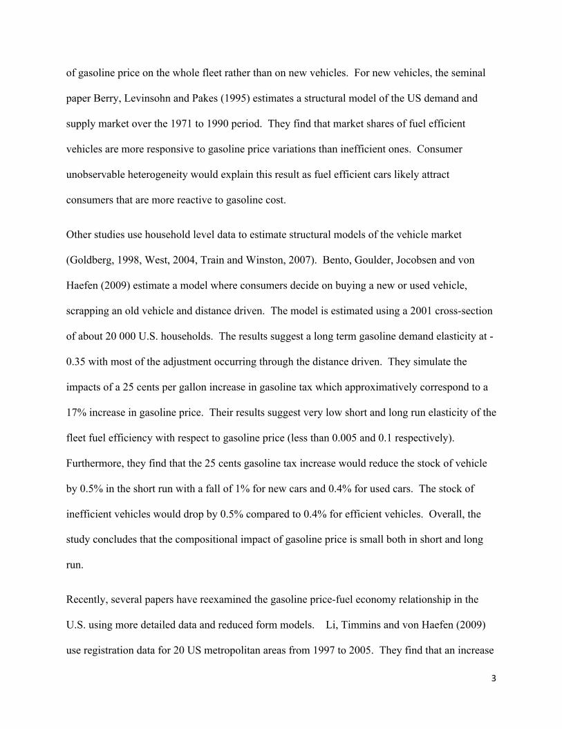
Figure 1 depicts kernel densities of the FCR for new vehicles registered in calendar year 2002
and 2008. The left panel illustrates the density of the available MY (309 MY in 2002 and 272 in
2008) while the right panel shows the density of new vehicles registered (i.e. each MY is
weighted by the number of new registrations). Both figures suggest fuel economy
improvements. On the supply side, the mode of the distribution remains centered at about
10L/100km but the density flattens with more efficient models being offered and less gas
guzzlers. On the demand side, the density of new registered vehicles clearly shifts left toward
more efficient vehicles. Interestingly, the average real price of gasoline was $1.11 in 2008
against 0.72$ in 2002.
Figure 1. Kernel density of fuel consumption rate (FCR) offered (left panel) and registered new vehicles (right panel) for calendar year 2002 and 2008.
Source: Authors’ calculations
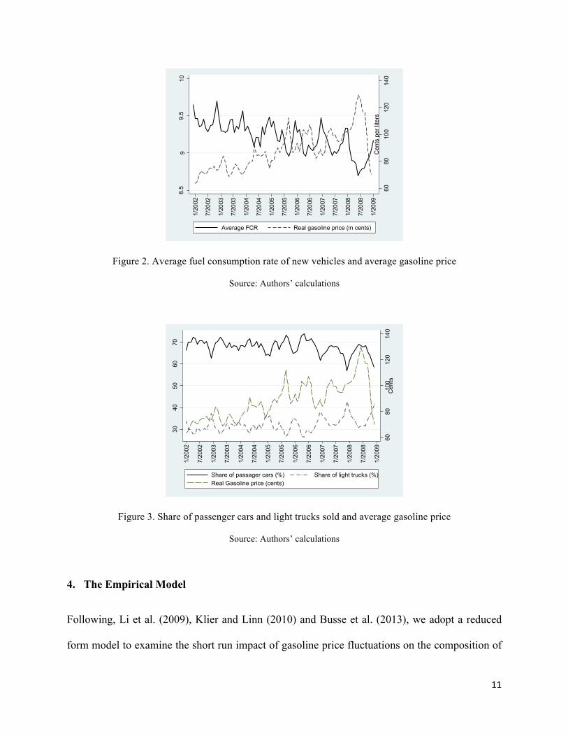
To explore further the potential impact of gasoline prices, Figure 2 illustrates the average FCR of
new vehicles sold each month and the corresponding monthly average gasoline price. We
0.0
5.1
.15
.2
FCR
ker
nel d
ensi
ty o
f mod
els
offe
red
5 10 15 20FCR
2002 2008
0.0
5.1
.15
.2.2
5
FCR
ker
nel d
ensi
ty o
f new
veh
icle
s re
gist
ered
5 10 15 20FCR
2002 2008
10
observe a general downward trend in the average FCR but also a negative correlation between
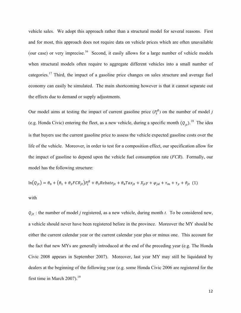
the price of gasoline and average FCR. Figure 3 also suggest that there is a positive correlation
between gasoline price and the share of passenger cars sold while the opposite occurs for the
share of light trucks. Still, the share of light trucks appears to be trending up at the end of the
period despite high gasoline prices. The share of light trucks was 31% in 2002 and close to 35%
in 2008. Moreover, the composition of sales in the light truck segment has been progressively
changing with a continuous decline of the van category (from 11% of the sales in 2002 to 5.9%
in 2008) and an increasing popularity of SUV (from 12.8% to 20%) and to a lesser extent of
pickups (from 6.3% to 7.9%). These observations suggest a concomitance of both short term
fluctuations associated with gasoline price and longer term changes due to technology and
preferences.15
In early 2007 the Canadian government announced a rebate program for efficient vehicles. From
March 2007 to December 2008, new car buyers could receive from 1000$ to 2000$ in rebate
when buying eligible vehicles. The rebates depend upon the fuel economy and the vehicle type.
For example, cars with a FCR of 5.5 L/100 km or less receive a rebate of 2000$, between 5.6 and
6L/100km, 1500$ and between 6.1 and 6.5L/100km 1000$. Flex fuel vehicles that consume less
than 13L/100 km were also eligible for a 1000$ rebate. The program only targeted MY2006 to
MY2008. In parallel, a new excise tax on fuel inefficient vehicles was introduced. It varied
from $1000 for vehicle with FCR between 14 and 15L/100km to $4000 for those with a FCR
above 16L/100km.
11
Figure 2. Average fuel consumption rate of new vehicles and average gasoline price
Source: Authors’ calculations
Figure 3. Share of passenger cars and light trucks sold and average gasoline price
Source: Authors’ calculations
4. The Empirical Model
Following, Li et al. (2009), Klier and Linn (2010) and Busse et al. (2013), we adopt a reduced
form model to examine the short run impact of gasoline price fluctuations on the composition of
6080
100
120
140
Cen
ts p
er li
ters
8.5
99.
510
Lite
rs p
er 1
00 k
m
1/20
02
7/20
02
1/20
03
7/20
03
1/20
04
7/20
04
1/20
05
7/20
05
1/20
06
7/20
06
1/20
07
7/20
07
1/20
08
7/20
08
1/20
09
Average FCR Real gasoline price (in cents)
6080
100
120
140
Cen
ts
3040
5060
70
1/20
02
7/20
02
1/20
03
7/20
03
1/20
04
7/20
04
1/20
05
7/20
05
1/20
06
7/20
06
1/20
07
7/20
07
1/20
08
7/20
08
1/20
09
Share of passager cars (%) Share of light trucks (%)Real Gasoline price (cents)
12
vehicle sales. We adopt this approach rather than a structural model for several reasons. First
and for most, this approach does not require data on vehicle prices which are often unavailable
(our case) or very imprecise.16 Second, it easily allows for a large number of vehicle models
when structural models often require to aggregate different vehicles into a small number of
categories.17 Third, the impact of a gasoline price changes on sales structure and average fuel
economy can easily be simulated. The main shortcoming however is that it cannot separate out
the effects due to demand or supply adjustments.
Our model aims at testing the impact of current gasoline price (𝑃!!) on the number of model j
(e.g. Honda Civic) entering the fleet, as a new vehicle, during a specific month (𝑄𝑗𝑡).18 The idea
is that buyers use the current gasoline price to assess the vehicle expected gasoline costs over the
life of the vehicle. Moreover, in order to test for a composition effect, our specification allow for
the impact of gasoline to depend upon the vehicle fuel consumption rate (FCR). Formally, our
model has the following structure:
ln 𝑄!" = 𝜃! + 𝜃! + 𝜃!𝐹𝐶𝑅!" 𝑃!! + 𝜃!𝑅𝑒𝑏𝑎𝑡𝑒!" + 𝜃!𝑇𝑎𝑥!" + 𝑋!"𝛾 + 𝜑!" + 𝜏! + 𝜏! + 𝜗!" (1)
with
𝑄!" : the number of model j registered, as a new vehicle, during month t. To be considered new,
a vehicle should never have been registered before in the province. Moreover the MY should be
either the current calendar year or the current calendar year plus or minus one. This account for
the fact that new MYs are generally introduced at the end of the preceding year (e.g. The Honda
Civic 2008 appears in September 2007). Moreover, last year MY may still be liquidated by
dealers at the beginning of the following year (e.g. some Honda Civic 2006 are registered for the
first time in March 2007).19

13
𝐹𝐶𝑅!": the average fuel consumption rate of all model j entering the fleet at t expressed in liter
per kilometer;
𝑃!!: the real average price of regular unleaded gasoline at time t in 2002$;
𝑅𝑒𝑏𝑎𝑡𝑒!": a binary variable equals to one if model j qualifies at time t for a rebate under the
Federal Auto feebate program;
𝑇𝑎𝑥!!: a binary variable equals to one if model j is taxed under the Federal Auto feebate program;
𝑋!" : other control variables. These include a set of 6 binary variables that controls for a
progressive increase in sales of new models. Specifically, 𝐼!"# equals 1 at time t if model j has
been first introduced i months ago with i=1 to 6. We also control for the progressive reduction in
sales for models that are programed to end. We thus introduced 𝐸!"# which is set equal to 1 at t if
model j is being retired in i months with i=1 to 6. Note that these variables only applied for the
introduction or retirement of a new model not a new model-year.20 We also control for time
varying economic indicators that may affect vehicles sales namely the level of income measured
by ln (𝑔𝑑𝑝𝑐𝑎𝑝!) the log of the gross domestic product per capita and ln(𝑖𝑝𝑒𝑟𝑠𝑜!) the log the
average interest rate on personal loans;
𝜑!": fixed effects for model j year d. As already mentioned, several MY of the same model may
be sold during the same month. For example, in October 2007, 1547 new Honda Civic were
registered in Quebec, 828 were MY 2007 and 719 MY 2008. We define the fixed effect 𝜑!"
using month t dominant MY. In our example, this means that the fixed effect 𝜑!" corresponding
to the 2007 Honda Civic is set to one. Alternatively, it is possible to assign to each 𝜑!" a value
that measures the share of MY d in the monthly total sales of model j.21 However, one issue with
14
this approach is that 𝜑!" may become endogenous as it is defined using 𝑄!". Thus our baseline
uses the dominant MY. The results obtained with the alternative specification are discussed in
section 6.
𝜏!: month-of-the-year fixed effects (m=1 to 12) to control for recurrent variations in sales across
the year;
𝜏!: year specific fixed effects (with y=2002 to 2008);
𝜗!": a random term that has the following structure 𝜗!" = 𝛿! + 𝜖!" with 𝛿! a month-of-data
specific random effects (with t=1 to 81) and 𝜖!" the usual error term. We assume that both terms
are normally and independently distributed with mean zero and variance 𝜎!! and 𝜎!! respectively.
We now explain in more details the main features of our empirical model. First, the impact of
gasoline price on sales is indeed allowed to vary with FCR which makes it possible to test for
changes in sales patterns across models with different fuel economy.22 For example, if a
gasoline price increase stimulates sales of efficient vehicles at the expense of inefficient ones, 𝜃!
should be positive and 𝜃! negative.23
Second, our model is static implying that consumers only react to current gasoline prices. This is
a very common hypothesis in the literature on the demand for new vehicles and consumer
valuation of energy efficiency investments. It is appropriate if gasoline prices follow a random
walk. While some empirical work provides support to this hypothesis (see Davis and Hamilton,
2004, German, 2007), recent studies seem to challenge it (e.g. Baumeister, Kilian and Lee,
2015). However, even if gasoline prices do not actually follow a random walk, our specification
is still adequate if consumers form their expectations about future gasoline prices using only the

15
current price (i.e. they act as if gasoline price follows a random walk). Recently, Anderson,
Kellogg and Sallee (2013) analyze this issue using the monthly Michigan Survey of Consumers.
This survey asks a representative sample of 500 respondents to forecast the price of gasoline
over a five year horizon. The results indicate that the average consumer forecasts no change in
real gasoline prices with respect to the current level thereby justifying our specification. There is
however one exception that is relevant for our analysis. Following the financial crisis, the price
of gasoline sharply dropped from September 2008 to December 2008 (see Figure 2). Anderson,
Kellogg and Sallee (2013) show that during that period, the average US consumers were
expecting a 15% to 20% rebound in gasoline prices. In other words during that period, current
gasoline prices were not a good measure of consumer expectations about future gasoline costs.
Moreover, the automobile industry was in deep turmoil during that period with great uncertainty
on the fate of several manufacturers. For these reasons, we eliminate the last three months of the
year 2008 in estimating our baseline model. In section 6, we explore the robustness of our
results to both the inclusion of past gasoline prices and the inclusion of the last three months of
2008.
Third, the fixed effects 𝜑!"control for model j characteristics as well as for the mean
characteristics of consumers buying this model. As models are updated annually these fixed
effects are also time dependant but with a time pattern that does not fit calendar year but rather
production cycle (thus subscript d is different than y). The specification also includes calendar
year specific effects to control for yearly variations in the car market. Hence, the identification
of the impact of the gasoline price rests upon the monthly relative variations in quantities across
models of different fuel economy. Moreover, the inclusion of month-of-the-year dummies
insures that these variations are not linked to recurrent seasonal patterns.

16
Fourth, we also account for the potential correlation in the quantities of the same month by the
inclusion of the random term 𝛿!. This correlation could result from month-specific unobservable
shocks that affect the LDV market. We treat this effect as random in order to be able to identify
𝜃!. This supposes the absence of correlation between 𝛿! and the explanatory variables
including 𝑃!!. While this hypothesis is debatable, it should be noted that our model includes time
specific variables which should hopefully limit the risk of bias due to unobservable factors. To
better access the results robustness to this hypothesis, we also present the estimations obtained
when polling the observations (i.e. ignoring 𝛿!) as well as those with 𝛿! included as fixed
effects.
Finally, it should be stressed that our analysis only measures the effect of gasoline prices on sales
conditional on the existing supply of vehicles (i.e. given the 𝜑!") . In that respect, we only
measure the short run effect of gasoline price. In the medium and long term, the characteristics
of the new vehicles proposed by manufacturers also response to gasoline price fluctuations
(Knittel, 2011).
5. Results
Table 1 presents the estimation results with column (1), (2) and (3) reporting the results obtained
without including 𝛿!, with 𝛿! as random and fixed effects respectively. We note very little
differences between the results in (1) and (2) except may be for the variable pibcap. While a
likelihood ratio test rejects the null hypothesis that 𝜎!!=0, it should be noted that 𝜎!! only account
for 2.3% of the total variance.24 Comparing (2) and (3), both specifications led to very similar
results for the variables that are common to both specifications.25 Obviously, this does not
guarantee that the coefficients for the time varying variables such as 𝑃!! are not biased by time-

17
specific unobservable factors. Still, the simulation results (discussed below) also lead to very
similar conclusions.
The main advantage of the random effects specification is that it allows to identify a threshold
FCR* such that sales of vehicles with a FCR below that limit increase with gasoline price while
the opposite occurs for values above that threshold. Based on Table 1 results, FCR* equals
8.65L/100km.26 The elasticity of the quantity sold with respect to the price of gasoline is given
by 𝜃1 + 𝜃2𝐹𝐶𝑅𝑗𝑣 𝑃𝑡𝑔. For a Toyota Corolla with a FCR of 6.5L/100km, the elasticity is 0.37 𝑃!
!
implying that a 10% increase in gasoline price around 1$/L stimulate sales by close to 4%. For a
Ford Taurus with a FCR of 10.2L/100km, the price elasticity is -0.27 𝑃!!. This suggests non-
negligible sale shifting following a change in gasoline prices at least for models with FCR very
different than 8.65L/100km. However, note that over 60% of new vehicles registered are within
a range of the threshold such as their elasticity is below 0.3𝑃!! in absolute value. Thus, for a
large share of vehicles, the impact of gasoline price on sales is not that high.
For comparison, recall that Li, Timmins and von Haefen (2009) find a threshold at 10L/100km
for the US. Also, the estimate for the coefficient 𝜃! can be directly compared to the estimate
obtained by Klier and Linn in the US. In the most comparable specification, they find an
estimate of -25.61.27 These comparisons suggest a somewhat smaller impact of gasoline price on
new vehicle efficiency in Quebec than in the US. This is likely due to the fact that the Quebec
sales are already oriented toward more efficient vehicles than in the US.

18
Table 1. Equation regression results (1) (2) (3) 𝑃!! 1.50*** 1.48*** -
(0.28) (0.27) 𝐹𝐶𝑅!"𝑥𝑃!
! -17.45*** -17.12*** -17.02*** (2.59) (2.08) (2.18) Rebate 0.19*** 0.17** 0.16* (0.06) (0.08) (0.08) Tax -0.04 -0.08 -0.09* (0.05) (0.05) (0.05) Ln(pibcap) 2.07* 1.16 (1.09) (2.17) - Ln(iperso) 0.22 0.21 (0.24) (0.43)
-
Entry and Exit dummies
yes yes yes
Model-year dummies
yes yes yes
Month of the year dummies
yes yes yes
Year dummies
yes yes yes
𝛿!
no random fixed
R2
0.90 - 0.90
𝜎! - 0.06 (0.006)
𝜎! - 0.42
(0.02)
LR test for 𝜎!=0
- 167.1 (p-value<0.0001)
Notes: the dependent variable is the logarithm of the monthly quantity of new vehicle registrations of a specific make-model. The number of observations is 14 734. The numbers in parenthesis are standard errors of the estimated parameter. For (1) and (3), we report the robust standards errors using Hubert-White sandwich estimators. For (2), the model is estimated by maximum likelihood. Coefficients for the fixed effects and those for the entry and exit dummies (I and E) are not shown. * Means statistically significant at the critical level of p < 0.1, ** at p < 0.05 and *** at p < 0.01.
Source: Authors’ calculations
19
Turning to the impacts of the feebate program, vehicles eligible to the rebate experience on
average a 17% increase in sales. On the other hand, inefficient vehicles that are surtaxed see
their sales reduced by 8 to 9%. This last effect is however only statistically significant in the
fixed effects specifications. The overall impact of the feebate program on fuel economy is very
small. Indeed, we compute that the average fuel economy would have been less than 1% higher
in the absence of this program. Moreover, this figure is likely an upper bound since it is derived
assuming that the rebate only generates additional sales.28 In reality, the rebate is likely shifting
sales at the expense of competing models that, even if they do not qualify for the rebate, are still
quite fuel efficient. While, it could be argued that the program created incentives for
manufacturers to improve fuel economy, this effect has most likely been very limited as the
rebate only lasted less than two years.29
Income per capita has a positive impact on sales but the effect is not statistically significant.
This is likely due to the lack of variability of this variable when year fixed effects are included.
The same is true for the interest rate on personal loans which do not even have the expected sign.
Finally, note that all the binary variables that control for the introduction and disappearance of
vehicle-models are statistically significant and have the right patterns (results available upon
request). Sales of new models gradually take off while those of disappearing models
progressively fade away.

20
Simulations
To gain a better insight on the magnitude of the overall composition effect, we simulate the
registration structure by vehicle category over the last 12 months of our sample period (October
2007 to September 2008) assuming that the price of gasoline had remained the same as in 2002
at $0.72.30 This actually corresponds to a 35% drop with respect to the average gasoline price
that was actually prevailing during this period. The results are reported in Table 2. The drop in
gasoline price would reduce by 11% the share of small and medium cars - the most fuel efficient
category. For intermediate and large cars, the reduction is somewhat smaller (-5%) while sport
cars experience a 10% increase in their share. Overall the share of passenger cars would drop by
7.7% from 65.1% to 60.1%. This corresponds to an arc elasticity of 0.18.31 At the opposite side
of the classification, the light truck segment sees its share increase by 16% from 34.5% to 40.1%.
The SUV and VAN shares both increase by about 10% while the pickup share jumps by 35%.
The average FCR of new LDV would increase by 3.6% following a 35% reduction in gasoline
prices implying an arc elasticity of about -0.08. More than two thirds of this increase is due to
changes in the sales structure across categories and less than a third to changes in sales pattern
within each category.32 Also note that the gasoline price decline would stimulate the overall
sales of new vehicles by about 2.5% suggesting an arc elasticity of -0.06. This is very close to
Bento et al. (2009) that finds that a 17% increase in gasoline price reduces sales of new vehicles
by 1% (i.e. an elasticity at 0.06).
Another worthwhile simulation exercise is to determine what the price of gasoline in 2008 would
need to have been so as to counteract the growing trend of light trucks. In the last 12 months of
our sample, the share of new registered light trucks was 34.5% compared to about 31% in 2002.
Gasoline price in 2008 would need to have been 1.4$/L to drive the share of light trucks down to

21
31%. This is a 26% increase with respect to the actual average price in 2008 and a doubling with
respect to 2002.
Overall, these results suggest a non-negligible sale shifting for vehicles that are at the extreme of
the fuel economy distribution, but for the bulk of vehicles the impact is far less important.
However, as gasoline price may experience large fluctuations, these may lead to noticeable
consequences on the composition of sales across vehicle classes. Still, the resulting impact on
the average fuel economy remains fairly modest. The corollary of these conclusions is that a
substantial gasoline price hike would be needed to neutralize the growing appeal of larger
vehicles.
Table 2. Simulated shares and average FCR for the period from October 2007 to September 2008 at actual and 2002 gasoline price
Category Shares with actual gasoline price
Shares with 2002 gasoline price
Average FCR with actual gasoline
price
Average FCR with 2002 gasoline
price CARS
65.1 60 7.69 7.78
Small-Medium 40.5 36.1 7.32 7.38 Intermediate-large 24.2 23.1 8.26 8.34
Sport cars
0.8 0.9 9.82 9.86
LIGHT TRUCKS
34.5 40.1 11.09 11.29
SUV 20.1 22.2 10.39 10.51 Van 6.4 7.1 10.44 10.48
Pickup
8 10.8 13.39 13.46
All LDV 100 100 8.87 9.19 The simulations are obtained using the coefficients of the random effects model.
Source: Authors’ calculations

22
6. Robustness Checks
In order to evaluate the robustness of our results, we investigate several alternative
specifications. In the baseline specification, we find a threshold FCR*=8.65L/100km but it
could be argued that this limit may have moved down over time with technological progress. To
examine this possibility, we reestimate the model on a subsample starting in 2006. The results
are summarized in Table 3. In fact, FCR* is somewhat larger at 8.9L/100km and the simulation
indicates a somewhat larger sale shift following a gasoline price drop.
Second, buying a new vehicle is a process that takes some time so that a moving average of the
price of gasoline during last three months before registering may be a better indicator for the
buyer anticipations about the future of gasoline prices. With this specification, the threshold
gets smaller at FCR*=7.5L/100km. The simulation results also indicate a somewhat larger
impact on the average FCR and the share of light trucks. We also explore the introduction of lag
values for the price of gasoline 𝑃! and the interaction term 𝐹𝐶𝑅!"𝑥𝑃𝑔. Using a general to
specific approach with a maximum of six months lags, the Schwarz’s Bayesian information
criteria is minimized at zero lag (i.e. the results reported in section 5). However, the Akaike’s
information criterion is minimized with three lags. The results with three lags are reported in
Table 3. The short run impact as measured by the coefficients on the current values is not that
different compared to the base specification. The cumulative effect following a long lasting
gasoline price decline suggests that almost all vehicles registrations increase (FCR*=4.72).
However, the impact is larger for vehicles with higher fuel consumption rates so that the
simulated share of light trucks (40.7%) and the average fuel rates (9.23l/100km) are not that
different than in the base model.33

23
Next, we explore the potential impact of the functional form by replacing 𝑃!! and FCR in
equation (1) by ln(𝑃!!) and ln(FCR). The results are relatively close to those obtained with our
original specification. We also estimate equation (1) separately on the subsample of passenger
cars and light trucks so that the determinants may have different coefficients for these two
categories (e.g. different seasonal pattern of sales). Figure 3 illustrates the impact of 𝑃!! on sales
as a function of FCR (i.e. 𝜃! + 𝜃!𝐹𝐶𝑅). The light truck segment appears somewhat more
reactive to gasoline price than the car segment but the overall pattern is similar and the
simulations in Table 3 are very close.
In our baseline specification, we use the dominant vintage to define 𝜑!". Alternatively, it is
possible to assign to each 𝜑!" a value that measures the share of MY d in the monthly total sales
of model j (see footnote 19 for an example). The results are robust to this specification change.
We also estimate the model with the data corresponding to the last three months of 2008 and thus
the sharp decline in gasoline price following the financial crisis. The results in Table 3 show that
the estimated threshold FCR* becomes quite large at 10.38L/100km which leads to the
questionable implication that a decline in gasoline prices lowers overall sales of vehicles. For
example, a decrease in gasoline price from 1.11$ to 0.72$ would result in a reduction of about
9% in total vehicle sales. This result is likely due to the unstable economic environment that
prevailed at the end of 2008 with low gasoline prices and depressed vehicles sales.34

24
Table 3. Alternative specifications results for the impact of gasoline price
Alternative specifications Simulation with 𝑃!!=0.72$ from
Oct. 2007 to Sept. 2008 𝜃! 𝜃! FCR* Av. FCR Share of light
trucks (1) Baseline 1.48*** -17.12*** 8.65 9.19 40.1 (2) 2006-2008 2.19*** -24.7*** 8.85 9.34 42.6 (3) Moving average 1.92*** -25.47*** 7.52 9.34 42.5 (4) Three lags model Current effect Lag one Lag two Lag three Cumulative effect(1)
1.25***
-0.30 0.15 -0.17
0.94***
-14.97***
-0.06 -2.45 -2.36
-19.84***
8.41
4.72
9.14
9.23
39.2
40.7 (5) Log-Log 4.04*** -1.85*** 8.87 9.27 41.5 (6) Passenger cars 1.13*** -13.42*** 8.43 7.76 Light trucks 2.23*** -23.23*** 9.62 11.38 38.7 All LDV 9.15 (7) Vintage -1.56*** -17.84*** 8.76 9.21 40.2 (8) Financial crisis 1.88*** -18.14*** 10.38 9.18 40 Notes: * statistically significant at the critical level of p < 0.1, ** at p < 0.05 and *** at p < 0.01. (1) The cumulative effects are the sum of the current and lag variables. The statistical significance of the cumulative effect is obtained using an F-test.
Source: Authors’ calculations
Figure 3. Impact of 𝑃!! on sales as a function of FCR with the base results and those on the subsamples of
passenger cars and light trucks
Source: Authors’ calculations
-2-1
01
impa
ct o
f Pg
5 10 15 20FCR
Passenger cars Light trucksall LDV (baseline specification)

25
As a last robustness check, we directly estimate the impact of gasoline prices on the average fuel
economy of new vehicles sold each month. This alternative model has the following structure:
ln 𝐹𝐶𝑅! = 𝜇! + 𝜇!𝑙𝑛𝑃𝑡𝑔 + 𝜇! ln (𝐺𝐷𝑃𝑐𝑎𝑝!) + 𝜇! ln (𝑖𝑝𝑒𝑟𝑠𝑜!) + 𝜇!𝐹𝑒𝑒𝑏𝑎𝑡𝑒! + 𝜏! + 𝜏! + 𝜗! (2)
In this setting, the variable Feebate is a binary variable which is set to one after March 2007
when the feebate program went into effect. The results of this model are reported in Table 4.
The elasticity of the FCR with respect to gasoline price is estimated at -0.08 which is identical to
our baseline finding. The simulated 2007-2008 average FCR with a gasoline price of 72 cents is
9.16L/100km which is also very close to our baseline.
All these alternative specifications confirm that gasoline prices have an impact on the
composition of new vehicles by fuel economy but with relatively modest consequences on the
average fuel economy. This conclusion is very much in line with recent US research.
Furthermore, the composition effect in Quebec appears somewhat smaller than in the US which
is likely due to the fact that Quebec fleet is already more efficient.

26
Table 4. Estimation results of equation (2)
Ln(FCR) Ln(𝑃!!) -0.08*** (0.01) Ln(pibcap) 0.17 (0.20) Ln(iperso) -0.06 (0.04) Feebate 0.00 (0.005) Year 2002 Ref Year 2003 -0.005* (0.003) Year 2004 -0.015*** (0.005) Year 2005 -0.013 (0.007) Year 2006 -0.017 (0.01) Year 2007 -0.015 (0.01) Year 2008 -0.036** (0.015)
R-square 0.93
N 81
In parenthesis, robust standard deviation
* p < 0.1, ** p < 0.05, *** p < 0.01
Source: Authors’ calculations
27
7. Conclusions
In this paper, we have evaluated the short term impact of gasoline price on the composition and
average fuel economy of new vehicles registered in the province of Quebec. We find a
statistically significant compositional effect: sales of efficient vehicles increase with gasoline
prices while the opposite occurs for the inefficient ones. While the impact is modest for the
majority of vehicles, a large gasoline price fluctuation can still lead to noticeable changes in the
structure of sales by vehicle classes. The impact on the average fuel economy of new vehicles
remains in any case rather modest. These results also imply that gasoline prices would have to
considerably increase to counteract the growing popularity of light trucks. In fact, we evaluate
that gasoline prices should have doubled for the share of light trucks in Quebec to remain stable
from 2002 to 2008.
We find that the impact of the federal feebate program between 2007 and 2008 increased sales of
low-fuel consumption eligible vehicles by 17% and decreased by 8 to 9% the sales of high-fuel
consumption cars. These tangible gains and losses in sales contrast with the overall impact on
fuel economy: it essentially remained unchanged. This was in part due to shifting sales from
close substitutes where one type of vehicle qualifies for a rebate and its sales increase at the
expense of very similar car models with a fuel economy just under the eligibility threshold.
Another factor is the short time span of the program of less than two years.
It is important to recall that in all our results we only measure short run effects, which are
essentially driven by the demand side. The medium and long run response of both consumers
and manufacturers remains to be better understood.

28
References
Anderson, S.T., R. Kellogg and J.M. Sallee (2013). What do consumers believe about future gasoline prices? Journal of Environmental Economics and Management, vol. 66, 383-403.
Barla, P., B. Lamonde, L. F. Miranda-Moreno and N. Boucher. (2009). Traveled distance, stock and fuel efficiency of private vehicles in Canada : price elasticities and rebound effect. Transportation, DOI 10.1007/s11116-009-9211-2.
Barla, P. (2011). Caractérisation énergétique et des émissions de gaz à effet de serre du parc de véhicules légers immatriculés au Québec pour les années 2003 à 2008, Rapport CDAT11-01, March 2011.
Barla, P., Lapierre, N., Daziano, R. and Herrmann, M. (2015). Reducing Automobile Dependency on Campus Using Transport Demand Management: A Case Study for Quebec City. Canadian Public Policy, 41(1), 86-96.
Barrington-Leigh, C., Tucker, B. and Kritz Lara, J. (2015). The Short-Run Household, Industrial, and Labour Impacts of the Quebec Carbon Market. Canadian Public Policy, 41(4), 265-280.
Baumeister C., Kilian L. and T.K. Lee (2015). New approaches to predicting the gasoline price at the pump, CFS Working paper series No. 500.
Bento, A. M., L. H. Goulder, M. R. Jacobsen and R. H. von Haefen. (2009). Distributional and Efficiency Impacts of Increased US Gasoline Taxes. American Economic Association, 99(3), 667-699.
Berry, S., J. Levinsohn and A. Pakes. (1995). Automobile Prices in Market Equilibrium. Econometrica, 63(4), 841-890.
Busse, M. R., C. R. Knittel and F. Zettelmeyer. (2013). Are Consumers Myopic? Evidence from New and Used Car Purchases. American Economic Review, 103(1), 220-256.
Davis M.C. and J.D. Hamilton (2004). Why are prices sticky? The dynamics of wholesale gasoline prices. Journal of Money, Credit and Banking, 36(1), 17-37.
Goldberg, P. K., (1998). The Effects of the Corporate Average Fuel Efficiency Standards in the US. The Journal of Industrial Economics, 46(1), 1-33.
Graham, D. J. and S. Glaister. (2004). Road Traffic Demand Elasticity Estimates: A Review. Transport Reviews, 24(3), 261-274.
Klier, T. and J. Linn. (2010). The Price of Gasoline and New Vehicle Fuel Economy: Evidence from Monthly Sales Data. American Economic Association, 2(3), 134-153.
Knittel, C. R. (2011). Automobiles on Steroids: Product Attribute Trade-Offs and Technological Progress in the Automobile Sector. American Economic Review, 101, 3368-3399.
Knittel, C.R. and K. Metaxoglou (2014). Estimation of Random-Coefficient Demand Models: Two Empiricists’s Perspective, Review of Economics and Statistics 96, no. 1, 34-59.

29
Li, S., C. Timmins and R. H. von Haefen. (2009). How Do Gasoline Prices Affect Fleet Fuel Economy? American Economic Journal: Economic Policy, 1(2), 113-137.
Mercier, X., Lanoie, P., and Leroux, J. (2015). Costs and Benefits of Quebec's Drive Electric Program. Canadian Public Policy 41(4), 281-296.
Miller J.D. and C. Façanha (2014). The State of Clean Transportation Policy: a 2014 Synthesis of Vehicle and Fuel Policy developments, The International Council on Clean Transportation.
National Archives and Records Administration (2010). Light-Duty Vehicle Greenhouse Gas Emission Standards and Corporate Average Fuel Economy Standards, Final Rule. Federal Register, May 7, 2010.
Natural resources Canada (2010). 2008 Canadian Vehicle Survey, Update Report, September 2010.
NHTSA (2012). Obama Administration Finalizes Historic 54.5 mpg Fuel Efficiency Standards, Press Release, August 28, 2012, Retrieved from http://www.nhtsa.gov/About+NHTSA/Press+Releases.
Small, K. A. and K. V. Dender. (2007). Fuel Efficiency and Motor Vehicle Travel: The Declining Rebound Effect. The Energy Journal, 28(1), 25.
Train, K. E. and C. Winston. (2007). Vehicle Choice Behavior and the Declining Market Share of U.S. Automakers. International Economic Review, 48(4), 1469-1496.
Transportation Research Board, Special Report 298. (2009). Driving and the Built Environment. The Effects of Compact Development on Motorized Travel, Energy Use, and CO2 Emissions.
Urmetzer, P., Blake D.E. and Guppy, N. (1999). Individualized Solutions to Environmental Problems: The Case of Automobile Pollution. Canadian Public Policy, 25(3), 345-359.
West, S. E. (2004). Distributional effects of alternative vehicle pollution control policies. Journal of Public Economics, 88, 735-757.
Wood, J. (2015). Is It Time to Raise the Gas Tax? Optimal Gasoline Taxes for Ontario and Toronto. Canadian Public Policy, 41(3), 179-190.
30
† The authors would like to acknowledge the financial support of the Institut Hydro-Québec Environnement, Développement et Société (Université Laval).
1 In Canada for instance, there exist proposed increases in gasoline taxes that fall short of the second-best levels (see Wood, 2015) and rebate programs to incentivize purchases of electric vehicles (see Mercier et al., 2015). Concerns about the externalities from automobile pollution in Canada have been present for several years (see Urmetzer et al., 1999). 2 See NHTSA (2012). 3 Other alternative instruments have also been put in place in Quebec such as the cap-and-trade program for emissions that is linked to California (see Barrington-Leigh et al., 2015). At a more local scale, there have also been efforts to reduce the use of vehicles when commuting but the impacts seem to be rather small (see Barla et al. 2015). 4 For example, D. Flavelle (2015), « Drivers trade up as gas price fall », Toronto Star, January 6, 2015 [Retrieved from: http://www.thestar.com/business/2015/01/06/drivers_trade_up_as_gas_prices_fall.html] 5 In the short run, manufacturers may, for example, adjust vehicle prices. 6 Light duty vehicles are those with a gross vehicle weight of less than 3855 kg (8500 lb.) or a curb weight of less than 2722 kg (6000lb.) (see Natural Resources Canada, 2008). 7 The sign of the elasticity is negative as we use the fuel consumption rate rather than MPG. 8 For a reason that will be clarified in section 4, our empirical model is estimated on data up to September 2008 i.e. just before the sharp drop in gasoline price caused by the financial meltdown. 9 These two protocols are those used in the US to assess compliance to the CAFE standards. They were developed in the late seventies and therefore do not represent very well actual driving conditions. These rates are thus adjusted upward following the procedure used by Natural Resources Canada (+22% for city FCR and +10% for highway FCR). 10 The last category includes subcompact, compact and two seaters that have a cylinder larger than three liters. 11 For the US, the comparison is based on fuel rates reported by manufacturers (USDOT National Transport Statistics Table 4-23 and US Census, Statistical Abstract 2012 Table 1069). For the comparison with the rest of Canada, the fuel rates are measured in actual driving conditions (see Natural Resources Canada, 2008). 12 For Canada and Quebec, the figures are for 2008 (Natural Resources Canada, 2010 and Barla, 2011). For the US, the figure is for the year 2012 (National Archives and Records Administration, 2010). 13 The quantile is defined on the supply of models available in 2008. 14 This figure is derived from table 7 of Busse et al. (2013, p. 238). It is based on national sales from 1999 to 2008. The quartile is redefined each year based on the available models. Comparable figures are unavailable for the rest of Canada. 15 Obviously the long term trends are also likely influenced by gasoline prices. 16 Very often only manufacturer suggested prices are available which may differ from actual transaction prices. 17 For example Bento et al. (2009) aggregate vehicles in 10 groups. Moreover, structural models à la Berry, Levinsohn and Pakes (1995) may pose serious problems of convergence as recently shown by Knittel and Metaxoglou (2014). 18 To simplify the presentation, we refer to a ‘model’ j when in fact it is technically a ‘make-model’ j. 19 Unfortunately, we cannot identify vehicles that were already registered in another province or abroad and thus are not new. This issue may be more problematic for MY corresponding to calendar year minus one. Thus, we impose that the registration of this type of vehicle should occur during the first quarter of the year to be considered as new. In other words, a 2006 Honda Civic registered in May 2007 is not considered new. 20 For example, the first registered Mazda 3 appears in November 2003. 21 Using the same example as before we would have for October 2007 𝜑!"#"$,!""# = ( !"!
!"#$) and 𝜑!"#"$,!""# = ( !"#
!"#$).
22 Li et al. (2009) use a similar functional form but to explain the quantity of vehicles by quantile of the FCR distribution. 23 Alternatively 𝜃! + 𝜃!𝐹𝐶𝑅!" 𝑃!
! can also be expressed as !!!"#!"
+ 𝜃! 𝑐𝑝𝑘!" with 𝑐𝑝𝑘!"= 𝐹𝐶𝑅!" 𝑃!! i.e. the fuel
cost of driving a km. 24 In fact, the random effect model has to be estimated by maximum likelihood as the GLS estimates lead to a corner solution with 𝜎!! =0.

31
25 As the random and fixed effects models have different regressors, the traditional Hausman specification test is not applicable. 26 This value is obtained by solving (1.48-17.13 FCR)=0. 27 We adjusted their coefficient to account for the difference in units (MPG versus L/km). 28 Indeed, our model does not allow us to identify the impact of the rebate on sales of competing models that are not eligible for the rebate. Some of this impact is however likely captured in the MY fixed effects. When simulating the impact of the rebate, we implicitly assume that the rebate only generates new sales which is obviously restrictive. The same is true for the tax. 29 The tax on inefficient vehicles is however still in place. 30 Recall that we eliminate the last three months of 2008 so that the last twelve months of our sample start in October 2007. 31 The arc elasticity is computed as follows: ((!"!!".!)/!".!)
((!.!!!!.!")/!.!")
32 To calculate these figures, we evaluate the average FCR using the category shares at actual price (column 2) but with the FCR by category at P=$0.72 (column 5). This leads to 8.94L/100km. Thus, the 3.6% increase can be decomposed in 2.8% due to variations in registrations across categories and 0.8% due to changes in registrations within each category. 33 Note that this specification implies a cumulative elasticity of the number of new registrations with respect to gasoline price of -0.7 which appears to be quite large. 34 In December 2008, sales were 35% lower than in December 2007 while gasoline price was 30% lower.