How does Private Equity Bid in Corporate Asset Sales?

by

Ulrich Hegea Stefano Lovob Myron B. Slovinc Marie E. Sushkad

Abstract

Wemodel the decision by private equity to bid for corporate assets, and analyze interactions betweenthe bidding of private equity and strategic buyers. The model predicts that seller gains depend onthe type of buyer. The aggressiveness of private equity bidding is related to expectations about itsability to enhance the value of the asset and to successfully exit from its investment. The model alsopredicts a relationship between the gains in the enterprise value of the asset while owned by privateequity, the type of exit transaction, and the gains to the original seller of the asset. Empirical testsshow that private equity deals generate greater seller returns relative to sales to strategic buyersand that the gains to �rms that sell assets to private equity are related to type of exit transactionand the subsequent increase in the asset�s enterprise value, which exceeds that of benchmark �rms.The evidence supports the view that private equity has valuable restructuring skills.

Keywords: Private Equity, corporate auctions, asset sales, secondary buyouts,restructuring.

JEL: G32, G34.

� � � � � � � � � � � � � � � � � �a Department of Finance, HEC Paris, hege@hec.frb Department of Finance, HEC Paris, lovo@hec.frc Department of Finance, HEC Paris, slovin@lsu.edud Department of Finance, Arizona State University, and HEC Paris, marie.sushka@asu.edu

How does Private Equity Bid in Corporate Asset Sales?

Abstract

Wemodel the decision by private equity to bid for corporate assets, and analyze interactions betweenthe bidding of private equity and strategic buyers. The model predicts that seller gains depend onthe type of buyer. The aggressiveness of private equity bidding is related to expectations about itsability to enhance the value of the asset and to successfully exit from its investment. The model alsopredicts a relationship between the gains in the enterprise value of the asset while owned by privateequity, the type of exit transaction, and the gains to the original seller of the asset. Empirical testsshow that private equity deals generate greater seller returns relative to sales to strategic buyersand that the gains to �rms that sell assets to private equity are related to type of exit transactionand the subsequent increase in the asset�s enterprise value, which exceeds that of benchmark �rms.The evidence supports the view that private equity has valuable restructuring skills.

Keywords: Private Equity, corporate auctions, asset sales, secondary buyouts,restructuring.

JEL: G32, G34.

How does Private Equity Bid in Corporate Asset Sales?

Since the early 1990s, private equity has become a major participant in �nancial markets and

an important bidder for corporate assets, an activity previously dominated by strategic buyers

(operating �rms). We develop an auction-based theoretical model and provide empirical results

that enhance our understanding of the role of private equity as bidders in corporate asset sales. We

address several key questions. One, how do private equity �rms decide whether to enter into the

competitive bidding for an asset, and how do the bidding behaviors of private equity and strategic

buyers interact? Two, how are the gains to �rms that sell assets a¤ected by the type of acquirer:

strategic buyer versus private equity? Three, for private equity deals, how are these gains related

to subsequent changes in enterprise value generated by private equity and its choice of exit route:

IPO, sale to a strategic buyer, or secondary buyout (sale to another private equity �rm)? Our

theoretical model generates an array of predictions that provide perspective on the role of private

equity in enhancing the value of corporate assets. We use a sample of large corporate asset sales to

empirically test the model�s predictions and provide evidence about fundamental issues relating to

private equity. Overall, our �ndings support the conclusion that private equity bids aggressively for

assets that are expected to generate important gains in value at exit, based on its ability to manage,

restructure, and improve these entities. We also �nd a pecking order in the predicted relationship

between the gains to the original seller, the asset�s performance while under private equity control,

and the type of exit transaction.

Corporate asset sales are a useful venue for analyzing the bidding behavior of private equity

and its competition with strategic �rms, because, unlike mergers, these transactions are invariably

non-hostile, are typically seller-initiated, and leave the selling �rm�s management team in place

1

after the transaction.1 Thus, it is logical to assume that a corporate seller seeks to structure the

sale process to spur competition between potential bidders that include both private equity and

strategic buyers. Moreover, the legal framework of asset sales allows a corporation to identify assets

for sale and to set the rules for an auction without reference to shareholder involvement or concerns

about legal actions where a court may be called upon to second-guess the merits of a decision. Thus,

our auction-based model closely conforms to the institutional framework governing asset sales.2

With regard to strategic bidders, our model applies the usual assumption that their bids re-

�ect the value of exogenous synergies between their assets and the asset for sale. However, with

regard to private equity bidders our theory endogenizes their decision to enter the bidding, and

the aggressiveness of their bidding is a function of their ability to enhance the value of the asset

and exit successfully. Although private equity bidders do not enjoy synergies, they may be able to

improve an operating asset in ways that are not feasible for strategic �rms or the parent seller. For

example, managers of lesser performing subsidiaries lodged within a parent organizational structure

have an incentive to lobby or in�uence parent decisions to secure additional resources to protect

their unit, costly activities, generally referred to as in�uence costs, that harm parent value (Meyer,

et. al., 1992). Private equity has the skills to eliminate such costs by altering strategies, devising

and implementing e¤ective restructuring plans, and enforcing management discipline. In addition,

private equity�s valuation of the asset depends on the expected revenue at exit and encompasses

expected synergies of future strategic bidders.3

1Eckbo and Thorburn (2008) report that on average asset sales make up 38% of all merger and acquisitiontransactions over the period from 1970 to 2006.

2The business judgment rule governs asset sale decisions, which gives managers broad discretion about the conductof the sale and insulates the transaction from shareholder voting and shareholder litigation. The laissez-faire approachof corporate law to asset sales is justi�ed since both seller and buyer managers continue to operate subject to thediscipline and monitoring of �nancial markets (Gilson, 1981).

3Since the sources of value for private equity versus strategic bidders are distinct and cannot be replicated bybidders belonging to the other buyer type, in auction parlance, the bidding competition between private equity and

2

Our analysis shows that when the expected gains for an asset are large, private equity is more

likely to enter the bidding and win the auction with relatively aggressive bids, whereas assets that

have lower restructuring potential are more likely to be acquired by strategic buyers for relatively

low bids. Thus, our theoretical model predicts that on average seller revenue is higher at news

of an asset sale to private equity compared to a strategic buyer. This prediction is in contrast to

prior empirical studies that consistently show that share price e¤ects and synergistic gains at asset

sales to strategic buyers are modest. In addition, for private equity deals, the gains to the parent

seller should be positively correlated with the expected subsequent performance of the asset, as

proxied by its ex post performance (measured as the annualized growth rate in enterprise value of

the asset at the exit transaction, a consistently observable metric). Our theory also predicts that

the subsequent performance of assets while under private equity management should exceed that

of benchmark �rms, and should also be related to the type of, and time to, the exit transaction.

Better exit performances and shorter times to exit should occur for IPOs, followed by sales to

strategic buyers, and then secondary buyouts. The reason that the gains in value should be greater

for trade sales compared to secondary buyouts is that after the asset�s restructuring by the original

private equity buyer, the marginal contribution of further restructuring rounds is relatively low,

implying that a subsequent private equity bidder is less able to compete with strategic bidders with

su¢ ciently strong synergies. Thus, a secondary buyout occurs when strategic bidder synergies are

low and the subsequent private equity acquirer acts as a form of buyer of last resort, expecting

to resell the asset when strategic bidder synergies are higher. In sum, the model suggests that a

secondary buyout is a less favorable form of exit than a sale to a strategic buyer or an IPO.

In practice, a strategic buyer may be either a public or a private operating �rm since each

strategic buyers is governed by a private values structure.

3

is motivated by expected synergies. However, private operating �rms are exempt from public

reporting and often have strong equity-based links between managers and owners, thus sharing

some of the characteristics of private equity. We provide insight about private strategic bidders by

analyzing the e¤ects on seller gains for each type of buyer.

We take our model to the data by analyzing large corporate asset sales from 1994 through

2004. Our main �ndings are broadly consistent with the bidding behavior of private equity implied

by our auction model. One, at asset sale announcements when the buyer is private equity, sellers

earn large positive excess returns, 3.78%, that are signi�cantly greater than when the buyer is a

public operating �rm, 1.25%, or a private operating �rm, 0.95%. We �nd a positive excess return

to public strategic buyers, 0.48%, suggesting an extraction of rents for their private information

about expected synergies and that their behavior does not entail the overbidding by acquirers that

Bargeron, et al. (2008) �nd in their study of mergers. Nevertheless, the overall level of synergies in

asset sales to strategic buyers is low, consistent with �ndings reported in prior asset sale studies.

The pattern of our results is similar when wealth gains are scaled by transaction size. The empirical

results indicate that private strategic buyers are similar to public strategic buyers.

Two, we assess whether the information conveyed at asset sales is asset-speci�c, as in our model,

or is more broadly applicable to the industry, by evaluating the e¤ect of these announcements on

industry values. We �nd no intra-industry gains, consistent with the view that the private infor-

mation conveyed by these deals is asset-speci�c and that a private values setting is an appropriate

framework for modelling corporate asset sales.

Three, we test whether seller gains at sales to private equity are related to the asset�s ex post

gains in enterprise value and to the type of exit transaction. Of the 146 assets sold to private equity

4

there are 121 with an exit (as of 2010). We con�rm the type of exit transaction and obtain the

enterprise value at exit. We evaluate the annualized change in the enterprise value of each asset over

the period it is owned by the original private equity buyer and �nd that on average it is signi�cantly

greater than its public benchmark �rm (matched by SIC code and enterprise value). These gains

are not a direct measure of pro�tability for investors in private equity funds, but they are a useful

metric of the business success of the entity while under private equity management. As our model

predicts, parent seller gains at the original sale are directly related to the form of exit and to the

subsequent gain in the asset�s enterprise value, with seller shareholders earning signi�cantly greater

gains in deals that exit by IPO or strategic asset sale rather than secondary buyout or bankruptcy.

Our evidence shows that private equity bids aggressively and generates large seller gains for assets

that subsequently prove to be a rich source of value, thus supporting the hypotheses that asset

sales can be plausibly modeled as auctions, that private equity buyers have e¤ective restructuring

skills, that private equity bids re�ect the expected gains from restructuring the asset, and that the

expected exit method and the time to exit are related to the magnitude of these gains.

Our analysis of exit type and subsequent changes in enterprise value contributes to the private

equity literature in a manner that di¤ers from prior studies, which focus on either the opera-

tional (performance) e¤ects of private equity activity or assessments of returns to fund investors,

studies that raise issues of selection bias in the data and that often generate ambiguous �ndings.

Several studies report evidence that �rms controlled by private equity improve their operating per-

formance, reduce employment, and lower capital investment relative to comparable public �rms

(Kaplan, 1989a, 1989b; Muscarella and Vetsuypens, 1990; Lichtenberg and Siegel, 1990; Liebe-

skind, Wiersema, and Hansen, 1992; Bharath, Dittmar, and Srivadasan, 2010). Other studies �nd

5

productivity changes at �rms owned by private equity are little di¤erent from comparable public

�rms, R&D investment is greater, employment tends to increase, and private equity�s governance

structure is highly e¤ective (Cornelli and Karakas, 2008; Lerner, Sorensen and Stromberg, 2009;

Leslie and Oyer, 2009; Guo, Hotchkiss, and Song, 2008). Recent studies of returns to fund investors

�nd few if any gains after adjusting for fees and write-downs (Kaplan and Schoar, 2005; Jones and

Rhodes-Kropf, 2004; Phalippou and Gottschalg, 2009).

Our formal treatment of the role of an informed buyer and the di¤erentiation of private equity

versus strategic buyers departs from prior asset sale studies, which do not provide any analytical

treatment of buyers and focus almost exclusively on the e¤ects on sellers (Jain, 1985; Hite, et

al., 1987; John and Ofek, 1995; Sicherman and Pettway, 1992). Overall, our work is consistent

with the view that private equity buyers have valuable skills in restructuring and value creation.

We argue theoretically and con�rm empirically that private equity is willing to generate higher

bids, producing economically important gains to sellers, when it expects to signi�cantly increase

an asset�s value, and that these gains are systematically related to the type of exit.

The paper is organized as follows. In Section I, our theoretical model is presented. Section

II describes sample construction. Section III contains empirical results for the valuation e¤ects of

asset sales, detailing the di¤erential e¤ects of alternative buyers. Conclusions are in Section IV.

I Theoretical Analysis

A. The Model Set-up

A.1 Asset

A parent �rm, the initial seller, is to sell an indivisible, tangible, productive asset with an

6

ascending bid auction. The asset has the potential to produce a constant and perpetual expected

cash �ow of c1, with a present value of v1 = �1�� c1. Under its current organization as a division

of the seller �rm, however, a per-period loss of c1 � c0 arises due to ine¢ ciencies in the current

organizational form.4 Thus, when remaining part of the seller �rm, the asset produces a net cash

�ow of only c0 < c1, with a present value of v0 = �1�� c0. We denote by Z = v1 � v0 > 0 the loss in

value due to these ine¢ ciencies.

A.2 Potential buyers

There are two di¤erent populations of potential buyers of the asset: private equity �rms, hence-

forth PEs, and operating �rms, henceforth strategic bidders or SBs. Within each population

category, the exact composition of the buyer pool varies over time.

Private equity: There are m PEs, where m > 1. PEs have a unique ability to restructure the

asset so as to increase its cash �ow, but achieve no operating synergies with the asset. A PE that

buys the asset will �rst restructure it and then sell it through an exit IPO or sell it to interested

parties through an exit auction. We denote by v0 + xPE the value of the asset to a PE buying

from the initial seller. The parameter xPE is endogenous in our model and depends both on the

potential operating performance of the asset following restructuring and on the expected market

value of the asset at the exit.

PEs can restructure the asset through two channels: one, by eliminating the loss in value Z

that the asset generates within the structure of a parent operating �rm, increasing the per-period

expected cash �ows from c0 to c1; two, by improving the asset�s operations, leading to an extra

4These ine¢ ciencies encompass in�uence costs that are generated by a division or subsidiary that undertakesnon-productive activities such as lobbying the parent for greater attention and seeking resources from the widerorganization, actions that attempt to bene�t the unit but that do not contribute to the value of the parent �rm as awhole.

7

increase from c1 to c2 > c1. The �rst component of gain encompasses the concept of the elimination

of in�uence costs; that is, there is some restructuring potential, Z, speci�c to the separation of an

asset from a parent that is not present in a merger. The second component of gain captures the

perspective that PE owners o¤er, for some �rms, unique capabilities of creating value that cannot

be replicated by other owners such as strategic buyers. The elimination of Z will be realized

with certainty during the �rst period of PE ownership. Thus, for simplicity the uncertainty about

restructuring outcomes is centered on the second component. In the �rst and any subsequent round

of PE ownership, with probability p the cash �ow can be permanently increased to c2, and hence

its present value to v2 = �1�� c2. With probability 1 � p the cash �ow remains at c1. Once v2 is

attained no further improvement is possible. Thus, the �rst restructuring round generates at least

Z = v1 � v0 whereas the expected number of restructuring rounds required to improve the asset�s

performance to v2 is 1=p. By the nature of a private equity deal, it is during the initial restructuring

round that the asset undergoes a substantial reorganization as it is transformed from a subsidiary

into an independent �rm, unlocking its potential value v1. Although subsequent restructuring

rounds may also generate positive bene�ts, they involve lesser restructuring. A PE incurs a one-o¤

cost of e < Z for the �rst restructuring e¤ort after it buys the asset, and we normalize to 0 the

cost of restructuring that occurs during each subsequent period of ownership of the asset by a PE.

Since the asset is taken private under PE ownership, we assume that only the PE owning the

asset knows whether the restructuring of the asset has achieved v2. In other words, at the time that

a PE exits the investment by selling the asset, the present value of the asset�s cash �ow, ev 2 fv1; v2g,is privately known to the PE. Although the main results of our model are not altered if we assume

heterogeneity with respect to the restructuring ability of PEs, we keep the theory more tractable

8

by assuming that these abilities are identical. That is to say, the parameters p, c0, c1, c2 and e do

not depend on the identity of the PE.

Strategic buyers: We assume that in every period t = 0; 1; :::, there is random draw of n > 1

new potential strategic buyers from a constant population, so that the distribution of potential

buyer characteristics is i.i.d. across time. This assumption captures the idea of a time-varying

set of strategic bidders. SBs have no special ability to restructure the asset. However, there are

synergies between the assets of the SBs and the asset for sale. For a given v 2 fv0; v1; v2g, that is,

the present value of the cash �ow generated by the asset, the valuation of the asset to a SB i is

equal to v + exi, where we denote by exi the idiosyncratic operating synergies between the assets ofSB i and the asset for sale. We assume that the synergies, exi 2 [xL; xH ], with xL � 0 < xH , areexogenous and private information to the strategic bidder i and that synergies are i.i.d. among the

SBs with c.d.f. F . We denote by ex(1) and ex(2) the �rst and second highest synergies among n SBs,respectively. Let F (�) be the c.d.f. of ex(�), for � = 1; 2. We assume that E[exi] > 0, implying thatthe expected synergies of SBs are positive. We allow for F (0) � 0, which implies that there can be

a strictly positive probability that in a given period t no SB is interested in acquiring the asset.

A.3 Timing and PE Exit

At time t = 0, the asset is sold in an auction with an ascending bid format and a starting

price of v0. Since the asset for sale is not publicly listed, a PE must �rst spend � > 0 in order to

identify and evaluate the asset and its potential p for improvement through restructuring. Each PE

simultaneously decides whether to invest � and participate in the auction or abstain from bidding.

Strategic buyers know their operating synergies and can participate without cost. If the asset is

sold to a strategic bidder i, it will become part of the buyer�s operating structure and generate cash

9

�ows with a present value of v0 + exi. If a PE participating in the auction, say PE j, acquires theasset, then the asset will �rst undergo restructuring; eventually, PE j will sell it again.

PE j will sell the asset either through an exit auction or through an exit IPO. In an exit auction,

the PE owner sells the asset in an auction with an ascending bid format. Potential buyers are PEs

and SBs. We assume that SB synergies are i.i.d. with the synergies of SBs participating in the

initial auction or any other subsequent contest for the acquisition of the asset. At the exit stage

the �rst PE�s restructuring of the asset has already increased the asset value to ev 2 fv1; v2g. Thus,if ev = v1, a PE buyer can improve the asset�s operating performance to v2, and eventually resell

the asset through a new exit auction or an IPO. At this stage the asset has been identi�ed as

restructurable so PE bidders do not need to invest � before bidding.

If PE j decides to exit via an IPO, then extensive disclosure requirements, the activity of stock

market analysts, and informed trading lead to a substantial reduction in asymmetric information;

we capture this e¤ect with the simplifying assumption that the asset�s true value ev will becomefully transparent in an IPO. It follows immediately that the PE�s revenue from the IPO, denoted

VIPO(ev), will re�ect the asset�s true pro�tability ev 2 fv1; v2g, and may incorporate an incrementre�ecting the possible future premium that would be paid in the event of a subsequent acquisition

by a strategic acquirer or a PE. Thus, we assume VIPO(ev) � ev.B. Equilibrium

We solve the game by backward induction. To proceed, we shall �rst determine the revenue

that PE j expects to receive once it owns an asset with performance ev = v1. Second, we deduce

v0 + xPE , i.e. PE j�s valuation of the asset in the initial auction. Third, we compute bidders�

expected equilibrium pro�t in the initial auction. Fourth, we compute the equilibrium entry decision

10

of PEs. This procedure allows us to analyze the seller�s expected revenue in the initial auction,

conditional on the winning bidder being a PE or a SB. We focus on symmetric equilibria.

The analysis is based on the claim (Claim 1 henceforth) that if a PE buys the asset, then at

the exit it will conduct an IPO if ev = v2 and it will auction the asset if ev = v1. Lemma 3 in theAppendix shows that this claim is correct in equilibrium if a takeover of the asset after the IPO is

possible among the same (random) set of buyers that participate in the exit auction.

B.1 IPO exit and exit auction

If PE j, after acquiring the asset and restructuring it, exits through an IPO, then the asset�s

true value will be fully disclosed in the IPO process and PE j�s revenue will be VIPO(ev) � ev.5Let VPE denote the expected cash �ow for a PE j that owns the asset whose current performance

is ev = v1 and will proceed to sell it in one time period. This value is computed at the beginningof a given period t and just after the asset has paid the cash �ow. Note that VPE also represents

PE j�s expected continuation payo¤ just after buying the asset from the initial seller and investing

e for restructuring it, but before observing the restructuring outcome. Then VPE must satisfy the

following equation:

VPE = �p(c2+VIPO(v2))+�(1�p) c1 +

Z minfxH ;VPE�v1g

xL

VPEdF(2)(x) +

Z xH

minfxH ;VPE�v1g(v1 + x)dF

(2)(x)

!:

(1)

This equation says that with probability p the asset�s operating performance improves in period t;

the PE will then receive c2 at the end of the period and immediately sell the asset through an IPO,

yielding an expected revenue of VIPO(v2). With probability 1 � p, the asset�s performance does5Note that in the case of an IPO, PE j will typically retain ownership of a fraction � of the asset; however, since

the IPO occurs at a fair price, PE j�s gain does not depend on �.

11

not improve in period t, and so the PE will receive c1 and will proceed to sell the asset through an

exit auction with an ascending bid format. Potential bidders in the auction include PEs and SBs.

Based on Claim 1, bidders will deduce that if PE j is exiting with an auction it must be ev = v1.The maximum bid that a PE k that is participating in the auction is willing to make for the asset

amounts to VPE . If in fact, PE k wins the auction (i.e., there is a secondary buyout), then it will be

in exactly the same situation as PE j is today. Note that PE j will not sell the asset for less than

VPE , since if today�s auction proceeds are less than VPE , PE j would rather continue restructuring

and retain the asset for one additional period. Thus, the exit auction will be won by the strategic

bidder with the highest synergies, provided that its synergies exi lead it to value the asset at morethan VPE ; i.e., v1 + exi � VPE . Otherwise, the asset will remain in the hands of a PE (either PEj or another PE buyer). Thus, the auction proceeds of PE j will correspond to the maximum of

the second highest bid and VPE . Let x denote the second highest synergy among the n strategic

bidders. Recall that its c.d.f. is F (2). The PE seller payo¤ is v1 + x > VPE only if the second

highest strategic bidder values the asset more than the PE bidders, which occurs for x > VPE � v1.

Otherwise, the seller�s expected proceeds is VPE . This reasoning suggests that in equilibrium in an

exit auction a strategic winner pays more than a PE winner. Thus, when a PE-owned asset (which

at this point is a stand alone entity) is auctioned o¤, we expect that the returns to the PE seller

will be greater on average when the asset is sold to a strategic buyer rather than to another private

equity �rm (a secondary buyout).

Note that there are two channels leading a PE to value the asset at VPE . One source of value

is the PE�s restructuring ability to achieve v2. The other source is the resale pro�t that a PE can

make when auctioning the asset, with performance v1, to SBs who enjoy synergies with the asset.

12

Let us �rst consider these two elements separately.

Suppose VPE > v1 + xH implying that no SB would ever have synergies that are high enough

to allow it to acquire the asset from a PE. In this case the asset will remain in PE hands until its

operating performance has been improved to ev = v2, at which point, it will be sold via an IPO. Interms of equation (1) this corresponds to the case VPE � v1 � xH and provides a VPE equal to

bVPE = � (p(c2 + VIPO(v2)) + (1� p)c1)1� (1� p)� � v1 ;

where the inequality is strict whenever p > 0.6 Thus, in the absence of SBs, a PE values the asset

more than v1 because of the potential for restructuring. Consider now the case where p = 0, i.e.

once v1 is achieved there is no prospect for further restructuring. By setting p = 0 and rearranging

equation (1) it can be shown that7

VPE jp=0 > v1 + �Ehmaxf0; ex(2)gi :

Moreover, in the limit we will have lim�!1 VPE jp=0 = v1 + xH . These expressions show that even

for an asset that cannot be restructured, a PE�s valuation is substantially higher than v1, provided

that there is a liquid exit market consisting of potential SB buyers and that the PE can continue

to hold the asset.

The following proposition describes VPE as well as the behavior of PE bidders and strategic

bidders in an exit auction.

6Note that bVPE = v1 for p = 0, which means that the value of the asset to a PE that has no synergies, thatwill never be able to improve the asset�s performance to v2 nor to sell it to SBs is equal to the present value of aperpetuity paying c1 in every period.

7 In this case the level of VPE � v1 that solves equation (1) is equal to the r solving r = �Ehmaxfr; ex(2)gi.

13

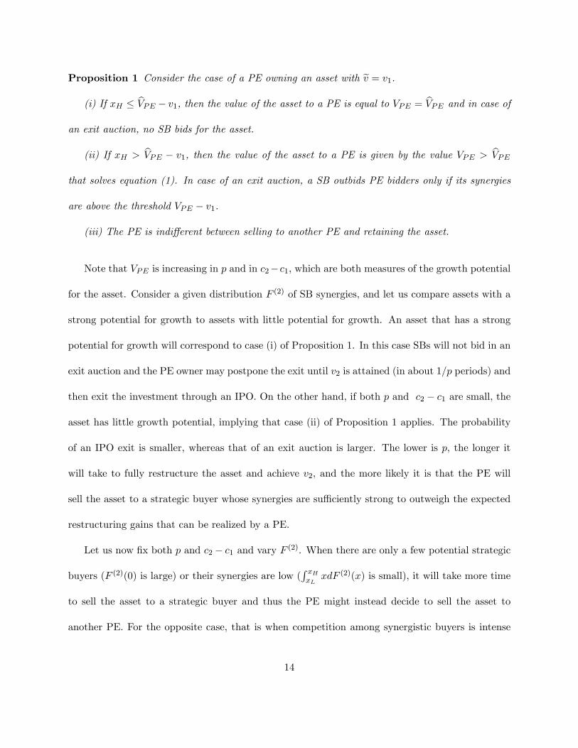
Proposition 1 Consider the case of a PE owning an asset with ev = v1.(i) If xH � bVPE � v1, then the value of the asset to a PE is equal to VPE = bVPE and in case of

an exit auction, no SB bids for the asset.

(ii) If xH > bVPE � v1, then the value of the asset to a PE is given by the value VPE > bVPEthat solves equation (1). In case of an exit auction, a SB outbids PE bidders only if its synergies

are above the threshold VPE � v1.

(iii) The PE is indi¤erent between selling to another PE and retaining the asset.

Note that VPE is increasing in p and in c2�c1, which are both measures of the growth potential

for the asset. Consider a given distribution F (2) of SB synergies, and let us compare assets with a

strong potential for growth to assets with little potential for growth. An asset that has a strong

potential for growth will correspond to case (i) of Proposition 1. In this case SBs will not bid in an

exit auction and the PE owner may postpone the exit until v2 is attained (in about 1=p periods) and

then exit the investment through an IPO. On the other hand, if both p and c2 � c1 are small, the

asset has little growth potential, implying that case (ii) of Proposition 1 applies. The probability

of an IPO exit is smaller, whereas that of an exit auction is larger. The lower is p, the longer it

will take to fully restructure the asset and achieve v2, and the more likely it is that the PE will

sell the asset to a strategic buyer whose synergies are su¢ ciently strong to outweigh the expected

restructuring gains that can be realized by a PE.

Let us now �x both p and c2 � c1 and vary F (2). When there are only a few potential strategic

buyers (F (2)(0) is large) or their synergies are low (R xHxLxdF (2)(x) is small), it will take more time

to sell the asset to a strategic buyer and thus the PE might instead decide to sell the asset to

another PE. For the opposite case, that is when competition among synergistic buyers is intense

14

and synergies are high, the PE will sell the asset relatively quickly to a strategic buyer, and for a

relatively high revenue.

B.2 Initial auction

From the previous section we are able to deduce that the maximum amount of money that PE

is willing to pay for the asset in the initial auction is VPE�e > v1 described in Proposition 1 which

corresponds to the present value of next period�s expected cash �ow and exit revenue, net of the

�rst restructuring cost e. Since they are homogeneous, all PEs value the asset at the same level.

We de�ne

xPE = VPE � e� v0 > 0

as the extra value a PE attaches to the asset compared to the value of the asset to the initial seller.8

By applying the implicit function theorem to equations (1) - (3) and by direct di¤erentiation of

bVPE , we can show that VPE is increasing in p, c1, c2, �, n and E [exi], i.e., the higher the growthpotential or the lower the cost of capital or the higher the number of potential SB buyers and their

expected synergies, the higher will be the value that a PE attaches to the asset for sale. Formally,

Corollary 1 In equilibrium, xPE is larger than �E[maxf0; ex(2)g] > 0 and is an increasing functionof p, c1, c2, �, n and E [exi].

The value of the asset for SB i is exogenous and equal to v0 + exi 2 [v0 + xL; v0 + xH ]. Thus, inthe symmetric equilibrium of the initial auction each bidder will increase its bid until it reaches its

own valuation of the asset. Since all PEs value the asset the same, as long as there are at least two

PEs in the initial auction they will bid up to their valuation and realize zero pro�t. Alternatively, a

8Note that VPE > v1 implies xPE := VPE � e� v0 > v1 � e� v0 = Z � e > 0.

15

PE that does not face competition from other PEs will pay the maximum between v0, the starting

price, and the highest SB valuation as long as this does not exceed v0 + xPE . In this case, its

expected pro�t is strictly positive and equal to9

��PE =

Z xPE

0(v0 + xPE � (v0 + x))dF (x)(1) + xPEF (1)(0) =

Z xPE

0F (x)(1)dx > 0:

B.3 PE entry decision

Let us now consider the decision of a PE to invest � and to bid for the asset in the initial

auction. Let x�PE be such that ��PE = �. The entry decision depends on whether other PEs enter

the auction or not. Lemma 1 describes the unique symmetric equilibrium of this entry game.

Lemma 1 In the unique symmetric equilibrium, the probability with which each PE participates in

the initial auction is q� = 1� (�=��PE)1

m�1 if ��PE > �, and 0 otherwise.

B.4 Seller revenue

Due to the fact that the valuation by PEs re�ects both the asset�s restructuring potential and

the synergies with a future SB buyer that are incorporated in the exit value, the economic forces

determining xPE suggest that xPE > E[exi]. Furthermore, the following proposition shows that�rst, the probability of a PE winning the initial auction increases with xPE ; second, that for xPE

large, the expected seller revenue from a winning PE bid is larger than the seller revenue from a

winning SB bid; third the same �nding is true if we compare the seller revenue from a PE bid when

xPE is large with the seller revenue from a SB bid when xPE is small. Formally, for a given level of

xPE , let RPE(xPE) and RSB(xPE) denote the seller�s expected revenue conditional on the winner

9Recall that starting bidding price is v0.

16

of the auction being a PE and a SB, respectively. Then we have:

Proposition 2 The probability of a PE winning the initial auction is increasing in xPE. There

exist thresholds xPE ; xPE, with x�PE < xPE < xPE < xH such that for xPE < xPE and x

0PE > xPE

we have RSB(x0PE) < RPE(x0PE) and RSB(xPE) < RPE(x

0PE).

As discussed earlier, a large xPE also means that it is more likely that a PE wins the initial

auction. That is, if we consider the comparative statics of the underlying parameters that drive

xPE according to Corollary 1, then the variation of any of the parameters p, c1, c2, �, n and E [exi]explains a correlation between the frequency of a PE outcome and the expected di¤erence between

a winning PE bid and a winning SB bid that increases as PE outcomes become more likely. We

will use this correlation in the discussion of empirical predictions to which we turn next.

C. Empirical implications

As our discussion prior to Proposition 1 shows, when p is positive and E�ex(2)� is not negligible,

a PE can enjoy both the gain from restructuring and the gain from the synergies of future SBs.

This suggests that for values of the parameters that are not extreme, on average a PE should value

the asset more than the average SB. As a consequence the seller expected revenue conditional on a

PE winning should be larger than the seller expected revenue conditional on a SB winning.

Let us then consider variations of the parameters p, c2, and Z that express PE restructuring

potential, as well as variations of the expected level of synergies among SBs, expressed by n and

E [exi]. Our model says that the PEs� endogenous value component, xPE , is increasing in theseparameters; the probability of a PE winning will increase in any of these parameters, and at the

same time the expected bid level of a winning PE bidder relative to that of a winning SB bid

will also increase. In other words, Proposition 2 shows that assets with a low PE value (low xPE)

17

are more likely to be sold to SBs, and to be sold to them at relatively low prices, while assets

with a high PE value (high xPE) are more likely to be sold to PEs, and at relatively high prices.

Thus, if we analyze a sample of assets with cross-sectional variation of the underlying parameters

discussed above, then this co-variation makes it likely that on average winning PE bids are higher

than winning SB bids. Since a measure of seller revenue is given by the seller�s abnormal return,

this analysis leads to our �rst set of empirical implications:

Empirical Prediction 1. The average abnormal return of the initial seller is higher when selling

to a PE compared with selling to a SB, under plausible parametric assumptions.

According to our model the improvement from v0 to v2 is only available if an asset is PE-

controlled, which by de�nition does not apply to a public benchmark �rm. Hence we should

observe:

Empirical Prediction 2. For assets acquired by PEs, the ex post performance of the asset until

exit (growth rate of enterprise value) should exceed that of a benchmark publicly traded �rm.

Empirical Prediction 3. If an asset is sold to a PE bidder, intra-industry rival �rms of the asset

should not exhibit any abnormal return reaction to the sale announcement.

According to our model, the most valuable assets to a PE are those with strong growth potential

and many potential synergistic buyers. After acquiring such assets a PE will quickly restructure

them and sell them through an IPO. The second most valuable assets are those that have smaller

growth potential but can have substantial synergies with future potential parents (strategic buyers).

When a PE buys this type of asset, it will be able to exit the investment relatively quickly through

an asset sale to a strategic buyer. Assets that are less valuable to a PE are those that are di¢ cult

to restructure and have few synergies with SBs. However, a PE can buy such an asset when there

18

are only a few bidders interested since it can acquire it for a relatively low price; but restructuring

the asset will be more time consuming and exit will tend to occur through a sale to another PE

that acts as buyer of last resort. It is also possible that these assets will culminate in Chapter 11.

This reasoning leads to the following empirical implications:

Empirical Prediction 4. The abnormal return of the initial seller should be positively correlated

with the expected performance of the asset, which can be gauged by the subsequent growth rate of

enterprise value.

Empirical Prediction 5. The performance of a PE owned asset is related to the choice of exit

route. The economic performance of the asset should be the highest when exit occurs through an

IPO, followed by a sale to a SB, and should be lowest in a secondary buyout. The expected time to

exit for the di¤erent exit routes is inversely related to the performance of the �rst PE owner.

Empirical Prediction 6. A PE receives a smaller revenue when exiting via a secondary buyout

compared to a trade sale.

II Sample

Our data set consists of corporate sales of large operating assets by publicly traded �rms obtained

from the SDC Acquisition Database for 1994 through 2004.10 We con�rm that each event is an

asset sale, and we identify the initial announcement date and obtain transaction data from sources

that include SEC �lings, Factiva, Lexis-Nexis, the Wall Street Journal, and Standard and Poor�s

Stock Reports, Stock Guide, and Directory of Corporations. Events are categorized by type of

buyer: private equity, public operating �rm, and private operating �rm. We verify that the assets

10Our sample goes through the end of December 2004 in order to have a su¢ cient period of time to observe exitsby private quity buyers.

19

sold are wholly-owned operating businesses of public (CRSP) �rms that are not in bankruptcy nor

divesting the asset due to a regulatory or judicial mandate. The identity of the acquirer and terms

of the transaction must be publicly reported and the transaction must transfer full ownership of

the subsidiary to the buyer. To minimize reporting bias, the minimum transaction price is $100

million, a condition that increases the probability that each asset is of su¢ cient size and stature to

be material, and that for sales to private equity the business is likely to warrant enough subsequent

interest in the business press to generate coverage of the date and type of exit transaction.

The �nal sample consists of 146 asset sales to private equity, 287 to public strategic buyers, and

48 to private strategic buyers. Descriptive statistics are shown in Table I. Values are reported in

constant (1997) dollars. These are large deals, with an average (median) transaction value of $398

($212) million for private equity, $644 ($255) million for public strategic buyers, and $308 ($222)

million for private strategic buyers. None of the di¤erences in means (medians) is statistically

signi�cant. Median transaction values are almost identical, suggesting that private equity has been

an e¤ective competitor in large asset sales. The mean (median) seller market capitalization is $22

($4.6) billion, $21 ($5.2) billion, and $8 ($2.6) billion in the respective subsamples; for public buyers

it is $22 ($2.7) billion. The three median ratios of transaction price to seller market value are of

similar magnitude. There is a broad range of industries given 105, 156, and 38 di¤erent 4-digit SIC

codes for the assets in the respective subsamples.

III Empirical Results

A. Valuation E¤ects of Corporate Asset Sales

In Table II, two-day market model average excess returns, proportion of returns positive, and

20

median returns at the initial sale announcement are reported. For asset sales to public strategic

buyers, seller excess returns are signi�cantly positive, 1.25%, t-statistic of 6.10 (median of 0.27%),

and similar to previously reported results (Jain, 1985; Hite, et al., 1987; John and Ofek, 1995;

Sicherman and Pettway, 1992; Hege, et al., 2009). The median transaction return, 2.85% (p = 0:29),

is reported to provide a metric for the economic importance of seller gains. As in previous studies,

the results show that the market views these asset sales as having positive net present value for

sellers, but the typical change in seller value is small relative to the size of the asset and is well

below the premiums of 25% or more observed for targets in merger studies.

For asset sales to private strategic buyers, seller excess returns are positive, 0.95%, t-statistic

of 2.19 (median of 0.46%), and not signi�cantly di¤erent from the result for public buyers. The

median seller transaction return, 3.68%, is similar to public buyer deals.

For asset sales to private equity, seller excess returns are positive and large, 3.78%, t-statistic

of 12.42 (median is 2.06%); the proportion of returns positive is 82%. The mean and median seller

returns are each signi�cantly greater than seller returns in deals with public buyers (p = 0:00), and

private operating �rms (p = 0:01). The median seller transaction return, 22.25% (p = 0:00), is also

signi�cantly greater than in deals with public or private strategic �rms (p = 0:00). This pattern

of seller returns is consistent with the prediction of our auction model and indicates the value of

private equity�s restructuring abilities.

Our �nding of greater returns to sellers when assets are sold to private equity is opposite to

Bargeron, et al. (2008) and Gorbenko and Malenko (2010). Bargeron, et al. (2008) report greater

gains (premiums) to merger targets acquired by public �rms, a result they ascribe to overbidding

that re�ects agency problems at public acquirers. However, we �nd positive average returns to

21

public strategic buyers in asset sales, 0.48%, t-statistic of 3.10 (median is 0.33%), implying they

extract a small rent for their private information about expected synergies. Thus, their behavior in

the aggregate is not characterized by overbidding or re�ective of agency problems (such as hubris

or empire building) as discussed in the merger literature (Thaler, 1988; Barberis and Thaler, 2003;

Baker, Ruback, and Wurgler, 2007). Nevertheless, the modest gains in combined shareholder wealth

at asset sales to strategic buyers imply that synergistic gains are modest, consistent with prior asset

sale studies cited earlier. Similarly, analyzing competitive auctions for entire �rms and not divisions,

Gorbenko and Malenko (2010) �nd that strategic buyers bid more, and display a greater dispersion

in winning bids. Since both studies analyze full-�rm mergers, possible restructuring gains from

eliminating in�uence costs of the subsidiaries we study are absent.

Our theoretical model implies that the return reaction of rivals (public �rms that are similar

to the asset being divested) should not be correlated with the excess return of the initial seller.

This prediction follows from the fact that the improvement in asset value from v0 to v1 and v2 is

only available for an entity controlled by private equity. Since �rms that are rivals of the asset are

not controlled by private equity, a winning private equity bid is not expected to have information

content for other �rms in the industry. We evaluate the intra-industry e¤ect of private equity bids

by examining share price responses of benchmark public �rms in the same industry with activities

similar to the asset sold. If a bid conveys new industry common information, then share prices

of benchmark �rms should increase at the sale announcement. We identify CRSP �rms with the

same 4-digit SIC code as the divested asset, construct an industry portfolio for each event (equally

weighting all rival �rms per event), and obtain the average portfolio excess return over all events

in each sample. The intra-industry e¤ects are small and not statistically signi�cant, implying that

22

there is little industry common information conveyed by an asset sale to private equity, or indeed

any asset sale irrespective of buyer type. This �nding supports the view that asset sale transactions

are appropriately modeled with a private values format.

B. Exit Transactions and Economic Performance for Private Equity Deals

Our auction model predicts that private equity bids are correlated with future revenues at

exit transactions, type of exit, and time to exit. Since the change in parent seller market value

at the initial sale announcement is in�uenced by the di¤erence between the price paid and the

market�s prior assessment of the asset�s value to the seller, parent returns should be related to

private equity�s expectations about its ability to generate value and exit the investment. Thus, if

ex post realizations and ex ante expectations are related, seller returns should be related to the

type of exit, the length of private equity ownership, and the ex post gains in asset enterprise value.

We investigate these predictions by determining the exit status (as of 2010) of each asset acquired

by private equity. Because the sample includes all large eligible operating assets sold by CRSP �rms

from 1994 through 2004, our �ndings about subsequent outcomes are not subject to selection bias

problems that are intrinsic to many studies of private equity due to lack of uniform disclosure

and the secretive nature of private equity �rms. Once acquired by private equity, the assets are

not public �rms and thus there is little disclosure about their operating performance or capital

structure, although the limited reporting available for our sample suggests that they are highly

levered while under private equity ownership. We identify the terms of the 121 exit transactions

and con�rm that each of the 25 assets without an exit remains a portfolio company of the original

private equity buyer.

In Panel A of Table III, the average time to exit is 3.4 years. We �nd that the time pattern of exits

23

closely matches the implications of the theory, which predicts that exit is most rapid when via an

IPO (2.1 years), longer via a trade sale (3.2 years), and longest via a secondary buyout (5.0 years).

For the secondary buyouts time to exit is signi�cantly longer than for IPOs (p = 0:00) and strategic

sales (p = 0:08). This evidence suggests that private equity sells an asset to other private equity

�rms when a timely exit via an IPO or trade sale is not feasible. As a result, secondary buyouts

may be regarded as less successful outcomes, or cases of incomplete restructuring, consistent with

our theory. For bankruptcies the time to exit is 4.4 years.

To determine the ex post (annualized) rate of increase in asset enterprise value while under

private equity ownership, we calculate transaction price, or market value of equity plus book value

of debt, depending on the type of exit transaction, and compare this value to the original sale

price. This metric is not a direct measure of pro�tability for fund investors, but it is a useful

gauge of an entity�s economic performance while under fund ownership. Our theory predicts that

the performance of the asset is related to the type of exit mechanism, with expected performance

highest for IPOs, next trade sales, followed by secondary buyouts. The data also allow us to test

the model�s prediction that the gains to the original parent �rm seller are greatest for deals that

exit via an IPO, and are greater for a strategic asset sale than a secondary buyout.

The mean (median) annual growth rate in enterprise value for the assets that exit is 48.45%

(18.69%). To benchmark our results, the annual growth rate in enterprise value over an identical

period is calculated for public �rms with the same 4-digit SIC code as the asset and are closest

in enterprise value to the original sale price. The mean (median) growth rate for the benchmark

�rms is 20.53% (6.12%) and the di¤erence in sample and benchmark �rm means (medians), Excess

EV, is statistically signi�cant, p = 0:00 (p = 0:00). Thus, the entities while owned by private

24

equity achieve considerable business success relative to benchmark �rms, consistent with the view

that private equity has valuable business skills. The changes in enterprise value at sample and

benchmark entities are highly correlated, 0.74, consistent with the expectation that an asset�s

growth opportunity is related to growth in the relevant industry, but the overall pattern of results

suggests that private equity has valuable skills that contribute to value, a portion of which is

received by the original sellers at the sale announcement.

We disaggregate the results by type of exit. Entities that �le Chapter 11 retain very little value,

given an average (median) annual decline in enterprise value of -27.11% (-21.20%). In principle,

private equity ownership could still increase an asset�s enterprise value despite a bankruptcy �ling,

as could be the case for a sustainable business that becomes overlevered, but is reorganized through

a negotiation between equity holders and creditors, either in the form of a prepackaged bankruptcy

or under the guidance of a bankruptcy judge.11 However, in our sample bankruptcy occurs after

almost complete business failure, resulting in the loss of the private equity stake and large losses

to unsecured creditors. Liquidation occurs in ten cases, with minimal payments to unsecured

creditors, and equity is cancelled (no payment to private equity). Reorganization occurs in eight

cases but almost all enterprise value is lost, with unsecured creditors absorbing large losses and

equity interests cancelled. In only two cases is there a reorganization in which some private equity

interests are conveyed to debtholders, resulting in a less levered entity that remains under private

equity control.

The systematic pattern to business success achieved by type of exit suggests a pecking order

with respect to gains in enterprise value that supports the predictions of our theoretical model. The

11For example, Kaplan (1989a) has argued that Campeau�s acquisition of Federated Department Stores added valueeven though it ended in bankruptcy.

25

highest mean (median) annual enterprise value growth rate occurs for IPOs, 111.52% (43.64%), and

is signi�cantly greater than benchmark �rms. The next highest mean (median) growth rate is exit

by sale to strategic buyers, 36.81% (24.78%), also signi�cantly greater than the growth rate of

their benchmarks. This estimate of the gains in enterprise value understates the overall (global)

economic gains since these transactions also add to buyer value. In 22 of the 37 deals where the

strategic buyers have CRSP returns, the buyer average excess return is 4.20% (p = 0:00), and the

average transaction return is 10.50% (p = 0:05); median returns are 2.96% (p = 0:00) and 7.75%

(p = 0:00), respectively. The positive buyer excess returns indicate that there is no evidence of

overbidding by public strategic buyers, just as in the case of asset sales as a whole.

Although secondary buyouts can be viewed as an alternative form of asset sale (where the

buyer is another private equity �rm rather than a strategic �rm), our theoretical model predicts

that in equilibrium a strategic buyer pays more than another private equity �rm at the exit auction.

The intuition for this prediction is that strategic bids encompass synergies that add value to the

restructured asset, synergies that are not available to private equity, together with the expectation

that the greatest improvements in restructuring the asset have already been carried out by the

original private equity �rm, leaving less scope for value creation by a second private equity owner.

Our model suggests that a private equity �rm is indi¤erent between keeping the asset or selling to

another private equity �rm. In actuality, private equity �rms are often under pressure to exit quickly

(Kaplan and Schoar, 2005) so secondary buyouts provide a means of exit when the termination

date of a private equity fund draws near and strategic buyers are scarce.

For the secondary buyouts, the mean (median) annualized growth rate in enterprise value is

20.48% (10.38%), signi�cantly less than for assets sold to strategic buyers, p = 0:09 (p = 0:05). This

26

�nding suggests that exit by secondary buyout is associated with poor performance of the asset

relative to assets that exit by IPO or strategic sale, although (median) performance is signi�cantly

(p = 0:05) more favorable than the gains achieved by benchmark �rms. We point out that the

greater gains in enterprise value when an asset owned by private equity (which like a target �rm

in a merger study is a stand-alone entity) is sold to a strategic buyer rather than to a second

private equity �rm, parallels results reported by Bargeron, et al. (2008) that there are greater

gains (premiums) to merger targets acquired by public �rms rather than private equity. They

attribute this result to overbidding by public buyers (due to agency problems). In contrast, our

theoretical model generates an explanation for this pattern of behavior for asset sale exits without

the presence of overbidding by public buyers. Moreover, our model suggests that when a private

equity �rm wins the exit auction, it will have less potential to improve the asset than the �rst

private equity buyer had. This reasoning implies that the asset�s performance during the second

buyout period should be no better than that during the initial round of private equity ownership.

To test this implication, we examine the outcomes for the secondary buyouts exits (as of 2010, 11 of

the 23 exit). In Panel B, performance during ownership by the second private equity �rm is broadly

similar to that of the initial private equity �rm. The second private equity �rm holds the asset for an

average of four years and the mean (median) annualized growth rate in enterprise value is 15.19%

(16.76%). Neither �gure is statistically di¤erent from the gains for the �rst private equity round.

Moreover, the second round gains di¤er little from the average (median) gains in enterprise value

of benchmark �rms, 14.92% (10.00%). This �nding is consistent with our model�s prediction and

at odds with the view that performance can be improved when an asset is transferred to another

private equity �rm that has some speci�c ability to improve the restructured asset that is not

27

available to the �rst private equity owner. We conclude that a secondary buyout is an unfavorable

form of exit relative to a sale to a strategic buyer or to an IPO.

The overall pattern of the growth in enterprise value for the benchmark �rms shows the same

rank order as the sample assets, with the highest growth rate for IPOs and the poorest for bank-

ruptcies. This evidence is consistent with the presumption that expectations about future industry

developments are a factor in the bidding behavior of private equity. Nevertheless, for each exit

category, except bankruptcies, the average (median) growth rate in enterprise value for assets orig-

inally acquired by private equity exceeds benchmark �rms, indicating the ability of private equity

to generate business improvements.

Consistent with our auction model, the pattern of gains to parent �rm sellers of assets parallels

the subsequent changes in exit enterprise value. Speci�cally, there are large statistically signi�cant

gains for assets that subsequently exit private equity via an IPO or a strategic asset sale, with

median transaction returns to the original sellers of 45.05% (p = 0:00) and 24.72% (p = 0:00),

respectively. By contrast, original sellers of assets that eventually sustain bankruptcy have a median

transaction return of 7.15% (p = 0:04), a �gure signi�cantly smaller than for IPOs (p = 0:05) or

strategic sales (p = 0:10). These results suggest that private equity submits lower bids when it

expects to generate modest gains, resulting in weaker gains to sellers. The median seller transaction

return for secondary buyout exits, 16.71% (p = 0:00), is smaller than for exits by IPO or sales to

strategic buyers, but greater than for Chapter 11 exits.

To further test the relationship between the excess return of initial sellers and subsequent asset

performance, we estimate regressions to control for other determinants of performance success,

Table IV, using a series of widely used measures. Our theory predicts that private equity bids, and

28

in turn seller excess returns, convey information about expected future payo¤s and private equity�s

ability to exit investments successfully. Our �rst dependent variable is the annual excess growth

rate in asset enterprise value (i.e., the di¤erence between the growth rates in enterprise values of the

asset and its benchmark). The coe¢ cient of the seller transaction return is positive and signi�cant,

suggesting that the seller�s share price reaction at an announcement of a private equity deal provides

a metric for the future success of the private equity investment. Our second performance metric is

a pro�tability index for which we obtain very similar results.12 In these regressions, there is some

evidence that deals that exited during the high tech bubble (1999-2001) generated lower gains in

enterprise value.

Our third performance measure is a binary variable of the relative eventual success of a private

equity deal, IPO or strategic asset sale, versus relative failure, bankruptcy or secondary buyout,

using a binomial logit model. The coe¢ cients for the seller transaction return are highly signi�cant,

providing an estimate as to how an increase in the transaction return for the parent �rm a¤ects the

marginal likelihood that an asset sold to private equity will exit via an IPO or strategic asset sale

rather than secondary buyout or bankruptcy. The qualitative variable for exit during the high tech

bubble years, while associated with lower growth rates in enterprise value, has a positive coe¢ cient

in the logit regression, suggesting exits by IPO and strategic sales were more likely during this

period. There is no evidence that the success of a private equity deal is related to transaction size.

Overall, the seller transaction return is signi�cant in all three speci�cations. These results are

consistent with a central implication of our theoretical model that private equity expectations about

future payo¤s a¤ect its bidding for an asset and the gains to selling �rms.

12The pro�tability index has been introduced in the literature to mitigate holding period biases typically presentin PE investments (e.g., Phalippou and Gottschalg, 2009).

29

C. Cross-sectional Regression Analysis

Overall, our results indicate a relationship between private equity outcomes and seller gains,

and a rank order for the types of transactions by which private equity exits an investment. The

large gains in enterprise value for the sample as a whole suggest that private equity has valuable

skills that are re�ected in its bidding behavior. We now use regression analysis to test whether other

factors, speci�cally observable seller or asset characteristics, a¤ect the statistically signi�cant seller

gains generated by private equity buyers. The dependent variable is de�ned as seller transaction

returns and alternatively, excess returns. In each regression, two qualitative variables for the type of

buyer are speci�ed. One variable takes on the value of unity for private equity and zero otherwise.

A second variable takes on the value of unity for private strategic buyers and zero otherwise. We

test an array of independent variables but, for economy of presentation, we report a representative

subset of regressions in Table V in which the dependent variable is the transaction return. The

pattern of results is similar when the dependent variable is seller excess returns. A full set of

regression results is available upon request to the authors.

The coe¢ cients of the qualitative variable for private equity are consistently large and signif-

icant, and are robust with respect to the inclusion of other variables that re�ect characteristics

of asset sales, including variables that have been considered in other studies of asset sales. Seller

variables reported include the size of the transaction relative to enterprise value, seller market

capitalization, prior cumulative stock price performance, operating performance (ROA), market to

book ratio, insider holdings, and use of proceeds (equal to one when used for debt reduction or

repurchase of equity, and zero for retention). The e¤ect of the variable for private equity buyers

remains positive and strongly signi�cant, irrespective of the regression speci�cation.

30

Other seller variables tested but not statistically signi�cant (results available upon request to

the authors) include leverage, dividend payout, time listed on CRSP, growth in intangible assets,

and measures of R&D. Alternative measures of size and capital structure do not alter the results.

Also we test variables that gauge focus, complexity, and opacity, including whether the asset has the

same SIC code as the parent (or public buyer), the number of seller business segments, the relative

importance of the segment in which the asset is sold, and whether the seller is a conglomerate.

Again, there is no evidence that the greater gains to seller �rms associated with private equity

deals are a¤ected by seller or asset characteristics.

Since Lewellen et al. (1989) suggests that high insider ownership mitigates agency problems

at buyers and Bargeron, et al. (2008) report greater returns to target �rms acquired by publicly

traded �rms with low insider ownership, we speci�ed variables for insider ownership of public

strategic buyers. We �nd no e¤ect of buyer insider ownership on seller returns (results available

upon request). Together with the positive excess return to strategic buyers, this result suggests

that bids by public acquirers do not re�ects buyer agency problems.

We investigate whether greater seller returns in private equity deals are related to �nancial

market conditions due to market timing opportunities given private equity funding cycles and

evidence that well-established funds bene�t from market �uctuations (Gompers and Lerner, 1998;

Gompers, et al. 2008; Ljungqvist, et al. 2006). We test variables for 1-year and 3-year lagged

performance of S&P500 and Nasdaq indexes, S&P500 operating performance, and dividend yields;

for debt markets, bond term spread and corporate credit spread; for exit markets, Fama-French

book-to-market ratio, number of IPOs, IPO �rst-day returns, and percentage of positive �rst-day

returns; and for the relationship of capital supply and capital disbursements, capital raised but not

31

invested by funds over the past �ve years. None of the variables is statistically signi�cant and the

qualitative variable for private equity deals remains consistently signi�cant, indicating the e¤ect of

the type of buyer for seller returns. We also test several variables to re�ect deals in which an asset

is acquired by the large, best known private equity �rms, but these coe¢ cients are not statistically

signi�cant, suggesting that identity of the private equity �rm does not a¤ect seller returns.

We estimate a binomial logit model of buyer type using the maximum likelihood method where

the value function for the logit is speci�ed as a linear function of asset- and �rm-speci�c variables,

plus an error term. The coe¢ cients indicate how a change in a speci�ed variable a¤ects the

marginal likelihood that an asset sold by a parent �rm will be acquired by a private equity buyer

(results are available on request). Our theory predicts that the level of strategic buyer synergies

and the potential for restructuring by private equity should be key factors relevant to the type

of winning buyer, although these factors are di¢ cult to observe and measure. In Table VI, we

test several factors that are observable to determine whether they have an in�uence on the type

of buyer. We �nd two signi�cant factors: one variable is a proxy for in�uence costs, and hence

the scope for restructuring of an asset; the other variable is a metric for the growing importance

of private equity in this sector of the corporate market. As an indicator of potential in�uence

costs, we specify a qualitative variable for selling �rms that are conglomerates (�rms with three

business segments or more). The coe¢ cient is positive, which suggests that a conglomerate structure

signi�cantly increases the likelihood of a private equity deal for the asset. In the internal capital

markets literature, in�uence costs generated by underperforming assets are viewed as more likely

to be high in the case of a broad based conglomerate (e.g., Scharfstein and Stein, 2000; Rajan,

Servaes, and Zingales, 2000). Thus, this result appears to be consistent with the view encompassed

32

in our model that when in�uence costs are high, the asset is more likely to be acquired by private

equity. We also specify separate variables for the e¤ect of transaction size before and after 2001

to capture the possibility that during the earlier years of the sample, the greater the size of the

transaction, the less the likelihood of a private equity deal; i.e., there was some constraint on the

ability of private equity �rms to �nance very large deals, re�ecting either the smaller size of these

�rms or the fact that consortia of private equity �rms had yet to become a major contender in this

market. The non-signi�cant coe¢ cient during the later period suggests that in recent years private

equity has had the capability of �nancing very large deals, so the size of an asset for sale has no

impact on the likelihood of a private equity deal.

Since the results of the logit regression indicate that buyer type is to some degree a function

of observable variables, we re-estimate the cross-sectional regressions for seller returns reported in

Table V, replacing the private equity dummy variable with two variables: (1) the �tted values from

the logit regression for buyer type, which can be interpreted as a proxy for the component of buyer

type that is related to variables that can be observed, and (2) the residuals from the logit regression,

which re�ect the impact of non-observable variables on buyer type. Within the framework of our

theory, we interpret these residuals as re�ecting the impact of private information conveyed by

the identi�cation of the type of buyer. The results indicate that it is the residual component that

is the signi�cant factor explaining seller returns (Table VII), while the observable component has

little impact (not reported in tables). These �ndings are consistent with a central prediction of our

theoretical model that it is private information conveyed by the acquirer type that in�uences the

level of the winning bid and the returns to sellers in corporate asset sales.

33

IV Conclusions

In this paper we analyze the participation of private equity �rms in the competition for corporate

assets. We develop an auction-type model of bidding competition that integrates the behavior

of private equity interests with that of strategic buyers, providing a theoretical framework that

conforms to the institutional structure of the asset sales market and the business model of private

equity �rms. In our auction model private equity�s valuation for the asset is endogenous, explained

by the fact that a private equity buyer can enhance asset value, and then exit the investment via

an IPO or an auction to a strategic buyer or another private equity �rm. In the model, competitive

bidding conveys private information about synergies held by strategic buyers as well as about the

participation of private equity bidders. We show that the gains in seller wealth are a¤ected by

the type of bidder. Our model predicts that average seller gains will typically be larger when

selling to private equity compared to strategic buyers in a sample composed of assets with varying

characteristics.

We test the empirical implications of the model by analyzing sales of large corporate operating

assets from 1994 through 2004, and follow the pattern of private equity exits through 2010. Sellers

earn large gains at sales to private equity, returns that are signi�cantly greater than for deals with

public or private strategic buyers. We �nd no intra-industry gains at news of asset sales, irrespective

of the type of buyer, suggesting that the information conveyed is asset-speci�c rather than having

industry-common elements.

We evaluate the change in the enterprise value of assets acquired by private equity over the

period from acquisition until the exit by the original buyer. We �nd that the annual growth rate in

the enterprise value of these assets is signi�cantly greater than for public benchmarks, suggesting

34

the economic importance of private equity�s business skills. We also determine the type of exit for

the assets acquired by private equity, where the majority are by IPO or strategic asset sale, with

a lesser percentage of secondary buyouts and bankruptcies. We �nd that the seller�s return at the

original asset sale announcement is directly related to the subsequent gain in enterprise value and

to the form of exit from private equity, with sellers earning a signi�cantly greater gain for assets

that exit by IPOs or a sale to a strategic buyer rather than by a secondary buyout. Thus, private

equity generates large gains in wealth for selling �rms in the case of assets that prove to be a rich

source of value for private equity. The results lead us to conclude that the ability to generate value

from an asset underlies the bidding behavior of private equity.

35

Appendix

Proof of Proposition 1: Observe that the maximum PE revenue from selling to a strategic buyer is

v1 + xH . For xH < bVPE � v1, this maximum revenue is less than bVPE , PE�s expected continuation payo¤obtained by never auctioning the asset and selling it via an IPO as soon as ev = v2. The case xH > bVPE � v1is an immediate consequence of the following Lemma:

Lemma 2 If xH > bVPE � v1, then equitation (1) has a solution satisfying bVPE < VPE < v1 + xH .Proof : Introducing the notation rauc = minfxH ; VPE � v1g, equation (1) can be restated in terms of

the following system of equations:

VPE = �

�p(c2 + VIPO(v2)) + (1� p)

�c1 +

Z rAuc

xL

VPEdF(2)(x) +

Z xH

rAuc

(v1 + x)dF(2)(x)

��;

(2)

v1 + rAuc � VPE = 0: (3)

Solving (2) in VPE leads to

VPE(rAuc) =��p(c2 + VIPO(v2)) + (1� p)

�c1 +

R xHrAuc

(v1 + x)dF(2)(x)

��1� (1� p)�F (2)(rAuc)

:

By substituting VPE(rAuc) for VPE in equation (3) we have

v1 + rAuc � VPE(rAuc) = 0: (4)

Then it is su¢ cient to show that there exists rAuc 2 [xL; xH ] that solves equation (4) and leads to

VPE(rAuc) > bVPE . Note thatVPE(rAuc)jrAuc=xL = �

�p(c2 + VIPO(v2)) + (1� p)

�c1 +

Z xH

xL

(v1 + x)dF(2)

��> �

�c1 + v1 + (1� p)

Z xH

xL

xdF (2)�� v1,

where the inequalities follow from c2 > c1, VIPO(v2) � v2 > v1,R xHxL

dF (2) = 1 andR xHxL

xdF (2)(x) =

E[ex(2)] � E[ex] > 0. Thus, the LHS of equation (4) is strictly negative for rAuc = xL � 0. Observe now thatVPE(rAuc)jrAuc=xH = bVPE . By substituting this expression into equation (4), we obtain that the LHS ofequation (4) is strictly positive for rAuc = xH if and only if xH > bVPE � v1. Hence, the system (2) - (3) has

a solution for rAuc 2]xL; xH [. Since VPE(rAuc) is decreasing in rAuc and VPE(rAuc)jrAuc=xH = bVPE > v1, itmust be that the VPE solving (1) satis�es bVPE < VPE < v1 + xH . �

This completes the proof of Proposition 1. �

36

Proof of Lemma 1: Note that if a PE j does not participate in the initial auction its payo¤ is nil

either because it will never buy the asset or because it will buy it at the fair PE value VPE from another

PE via an exit auction. If PE j invests � to participate to the initial auction, then its payo¤ is ��+ ��PEif it is the only PE bidder and �� otherwise. If ��PE < �, no PE will ever invest � and the resulting q� isnil. Consider the case ��PE � � and let q be the mixed strategy entry probability adopted by each of the

other m� 1 PE in a symmetric equilibrium. Then PE j is indi¤erent between entering or not if and only if��+ (1� q)m�1��PE = 0, which is true for q = q�. �

Proof of Proposition 2: For a given xPE , the probability of a PE winning the initial auction is

F (1)(xPE)(1� (1� q�)m), that is the probability that the highest of SBs bidder�s synergies is less than xPEtimes the probability that at least one PE participates to the auction.

Consider �rst RPE(xPE). The PE wins only if the highest value of synergies among SBs is less than xPE .

If the winning PE faces no competition from other PEs, then it will pay the highest of the SBs�valuations,

for which the expectation, conditional on PE winning the auction, is v0 + E[ex(1)�� ex(1) < xPE ]. If there is

at least one other PE bidder, then the winning PE will have to pay v0 + xPE . It immediately follows that

RPE(xPE) can be expressed as

RPE(xPE) = v0 + �E[ex(1)��� ex(1) < xPE ] + (1� �)xPE ,where � 2]0; 1[ only depends on q�. Clearly, RPE(xPE) is continuous and increasing in xPE equal to

v0+ �E[ex(1)] + (1� �)xPE for xPE � xH . Consider now RSB(xPE). If a SB faces no competition from PEs,

then it will pay the highest of other SBs valuations, that in expectation equals v0 +E[ex(2)]. If a SB wins inthe presence of PEs, he will pay the maximum between the highest of the other SBs�valuations and xPE ,

which in expectation is v0 + E[ex(2)�� ex(2) > xPE ]. Note, however, that when xPE increases, a SB will tendto win only when facing no competition from PEs. Hence we can write

RSB(xPE) = v0 + (xPE)E[ex(2)] + (1� (xPE))E[ex(2)��� ex(2) > xPE ] ,where (xPE) increases with xPE and tends to 1 as xPE approaches xH . Thus, we have RSB(0) =

RSB(xH) = v0 + E[ex(2)]. Since RSB(xH) < RPE(xH) the result follows from the continuity of RSB and

RPE . �

Veri�cation of Claim 1: Let VAuc(ev) denote the PE expected revenue from an exit auction whenev 2 fv1; v2g. We say that the takeover market for the asset after its IPO is open if in every period a takeovercontest for the asset is possible among a set of buyers randomly drawn from the same buyer population as

in the exit auction described in the model. It is su¢ cient to show that in equilibrium the following lemma

holds:

Lemma 3 If the takeover market for the asset after its IPO is open, then in equilibrium VIPO(v2) > VAuc(v2)

and VAuc(v1) > VIPO(v1).

37

Proof : We �rst show that VAuc(v1) > VIPO(v1). Note that PE bidders�value of the asset when ev = v1is VPE , whereas SB i values the asset v1 + exi. Hence if PE j auctions the asset its expected revenue can bewritten as

VAuc(v1) = Ehmax

nVPE ; v1 + ex(2)oi > v1 ,

where the inequality follows from VPE > v1 and E�ex(2)� > 0. If PE j sells the asset via an IPO, then its

true value ev = v1 will be publicly known at the time of the IPO. Then, the asset will be subject to a takeovercontest by the same expected set of PEs and SBs that would participate today if the asset were auctioned.

Hence today�s revenue from the IPO satis�es

VIPO(v1) � ��c1 + E

hmax

nVPE ; v1 + ex(2)oi�

< Ehmax

nVPE ; v1 + ex(2)oi = VAuc(v1).

To see that VIPO(v2) > VAuc(v2) note �rst that VAuc(v2) = VAuc(v1). This is because from the fact that

PE j auctions the asset, bidders deduce that ev = v1 and their bids will re�ect this belief. It is then

straightforward to see that VIPO(v2) > VAuc(v1). In fact, VIPO(v2) re�ects the expectation of the synergies

of future strategic acquirers plus the present value of the asset�s maximum possible cash �ow, v2. Similarly,

the revenue VAuc(v1) re�ects the synergies of future strategic acquirers; however, at the moment of bidding

the expected value of future cash �ows is strictly less than v2. �

38

References

Baker, M., R. Ruback, and J. Wurgler, 2007, Behavioral corporate �nance: A survey, in Handbook

of Corporate Finance: Empirical Corporate Finance, edited by E. Eckbo, Elsevier/North-Holland.

Barberis, N. and R. Thaler, 2003, A survey of behavioral �nance, in Handbook of the Economics

of Finance, edited by G. Constandinades and M. Harris, Elsevier/North-Holland.

Bargeron, L., F. Schlingemann, R. Stulz, and C. Zutter, 2008, Why do private acquirers pay so

little compared to public acquirers? Journal of Financial Economics 89, 375-390.

Bharath, S., A. Dittmar, and J. Srivadasan, 2010, Does capital market myopia a¤ect plant produc-

tivity? Evidence from �going private�transactions, Working paper, University of Michigan.

Cornelli, F. and O. Karakas, 2008, Private equity and corporate governance: Do LBOs have more

e¤ective boards? Unpublished working paper, London Business School.

Eckbo, E., and K. Thorburn, 2007, Corporate restructuring: Breakups and LBOs, in Handbook

of Corporate Finance: Empirical Corporate Finance, edited by E. Eckbo, Elsevier/North-Holland.

Gilson, R., 1981, A structural approach to corporations: The case against defensive tactics in tender

o¤ers, Stanford Law Review 33, 819-851.

Gompers, P., and J. Lerner, 1998, What drives venture capital fund raising? Unpublished working

paper, Harvard University.

Gompers, P., A. Kovner, J. Lerner, and D. Scharfstein, 2008, Venture capital investment cycles:

The impact of public markets, Journal of Financial Economics 87, 1-23.

Gorbenko, A.S. and A. Malenko, 2010, Strategic and �nancial bidders in takeover auctions, Un-

published working paper, Stanford University.

Guo, S., E. Hotchkiss, and W. Song, 2008, Do buyouts (still) create value? Journal of Finance,

forthcoming.

39

Hege, U., S. Lovo, M. Slovin, and M. Sushka, 2009, Equity and cash in intercorporate asset sales:

Theory and evidence, Review of Financial Studies 22, 681-714.

Hite, G., J. Owers, and R. Rogers, 1987, The market for inter�rm asset sales: Partial sell-o¤s and

total liquidations, Journal of Financial Economics 18, 229-252.

Jain, P., 1985, The e¤ect of voluntary sell-o¤ announcements on shareholder wealth, Journal of

Finance 40, 209-224.

John, K., and E. Ofek, 1995, Asset sales and increase in focus, Journal of Financial Economics 37,

105-126.

Jones, C., and M. Rhodes-Kropf, 2004, The price of diversi�able risk in venture capital and private

equity, Unpublished working paper, Columbia University.

Kaplan, S., 1989a, Campeau�s acquisition of federated: Value destroyed or value added? Journal of

Financial Economics 25, 191-212.

Kaplan, S., 1989b, The e¤ects of management buyouts on operating performance and value, Journal

of Financial Economics, 24, 217-254

Kaplan, S., and A. Schoar, 2005, Private equity performance: Returns, persistence, and capital

�ows, Journal of Finance 60, 1791-1823.

Kaplan, S., and P. Stromberg, 2009, Leveraged buyouts and private equity, Journal of Economic

Perspectives 23, 121-146.

Lerner, J., M. Sorensen, and P. Stromberg, 2009, Private equity and long run investment: The

case of innovation, Unpublished working paper, Harvard University.

Leslie, P., and P. Oyer, 2009, Managerial incentives and value creation: Evidence from private

equity, Unpublished working paper, Stanford University.

Lewellen, W., C. Loderer, and R. Roenfeldt, 1989, Mergers, executive risk reduction, and stock-

holder wealth, Journal of Financial and Quantitative Analysis 24, 459-472.

40

Lichtenberg, F. and D. Siegel, 1990, The e¤ects of leveraged buyouts on productivity and related

aspects of �rm behavior, Journal of Financial Economics 27, 165-194.

Liebeskind, J., M. Wiersema, and G. Hansen, 1992, LBOs, corporate restructuring, and the

incentive-intensity hypothesis, Financial Management 21, 73-88.

Ljungqvist, A., V. Nanda, and R. Singh, 2006, Hot markets, investor sentiment, and IPO pricing,

Journal of Business 79, 1667-1702.

Maksimovic, V., and G. Phillips, 2001, The market for corporate assets: Who engages in mergers

and asset sales and are there e¢ ciency gains? Journal of Finance 57, 721-767.

Muscarella, C., and M. Vetsuypens, 1990, E¢ ciency and organizational structure: A study of

reverse LBOs, Journal of Finance 45, 1389-1414.

Phalippou, L., and O. Gottschalg, 2009, Performance of private equity funds: Another puzzle?

Review of Financial Studies 22, 1747-1776

Rajan, R., H. Servaes, and L. Zingales, 2000, The cost of diversity: The diversi�cation discount

and ine¢ cient investment, Journal of Finance 55, 35-84.

Scharfstein, D. and J. Stein, 2000, The dark side of internal capital markets: Divisional rent-seeking

and ine¢ cient investment, Journal of Finance 55, 2537-2565.

Sicherman, H., and R. Pettway, 1992, Wealth e¤ects for buyers and sellers for the same divested

assets, Financial Management 21, 119-128.

Thaler, R., 1988, Anomalies: The winner�s curse, Journal of Economic Perspectives 2, 191-202.

41

Table I Descriptive Statistics

Statistics for means, and medians in parentheses, are reported for asset sales of $100 million or more conducted by publicly traded sellers listed on NYSE/ASE/Nasdaq over the sample period 1994 through 2004, obtained from the SDC Acquisition Database. Transactions are disaggregated on the basis of the type of buyer into 146 asset sales to private equity buyers (PE), 48 asset sales to private strategic buyers (private operating firms), and 287 asset sales to publicly traded strategic buyers. The value of the transaction is reported in millions of constant (1997) dollars. Firm market value is calculated as the number of shares outstanding multiplied by stock price prior to the event announcement, and reported in millions of constant (1997) dollars.

Private Equity Buyer Strategic Private Buyer Strategic Public Buyer

Seller Seller Seller Buyer

N=146 N=48 N=287 N=287 Transaction value ($1997, m) 397.90 308.12 643.73 643.73 (211.81) (222.25) (255.00) (255.00) Market value ($1997, m) 21,694.95 7,817.36 20,721.6 22,184.96 (4,614.09) (2,560.66) (5,228.31) (2,677.25) Asset/MV 0.26 0.52 0.31 0.34

(0.07) (0.09) (0.07) (0.11)

Table II Empirical Results for Share Price Responses at Asset Sales

Empirical results are reported for excess returns at asset sales of $100 million or more conducted by publicly traded sellers listed on NYSE/ASE/Nasdaq over the sample period 1994 through 2004, obtained from the SDC Acquisition Database. The metrics are two-day (-1, 0) announcement cumulative excess returns (CARs) for sellers and for publicly traded buyers (Panel A) and two-day median transaction returns (TR), measured as the dollar gains in value scaled by transaction value (Panel B). Excess returns and transaction returns in percent are in response to 146 asset sales to private equity firms (PE), 287 asset sales to publicly traded strategic buyers (Public SB), and 48 asset sales to private strategic buyers (Private SB). To obtain rival CARs, CRSP firms with the same 4-digit SIC code as the asset are used to form an industry portfolio for each event (equally weighting rival firms per event), and then are averaged over all events. Combined returns weight the buyer and seller returns by market capitalization. Excess returns are calculated using market model methodology; t-statistics are in parentheses, proportion of returns positive is in brackets. Median returns are in braces. The statistical significance of median returns is based on the Wilcoxon signed ranks test. Statistical significance for the difference between types of buyers is obtained by the Satterthwaite test for the difference in means and by the Wilcoxon signed ranks test for the difference in medians. Market model parameters are estimated using least squares over the pre-event period, t = -160 to -41, where day 0 is the date of the first public announcement. Statistical significance is denoted as: *** for the 1% level, **, for the 5% level, and *, for the 10% level. .

Private Equity Buyer

Strategic Public Buyer

Strategic Private Buyer

p-difference in means {medians} Strategic Public Buyer

Seller Seller Seller PE /

Public SB PE /

Private SB Public SB / Private SB

Buyer Combined

N=146 N=287 N=48 N=287 N=287 Panel A: Excess Return

Two-day CAR (-1, 0) 3.78% 1.25% 0.95% 0.00 0.01 0.81 0.48% 0.31% (12.42)*** (6.10)*** (2.19)** (3.10)*** (1.40) {2.06%}*** {0.27%}** {0.46%} {0.00} {0.00} {0.78} {0.33%} {0.32%} [0.82] [0.54] [0.52] [0.55] [0.54]

Rival CAR (-1, 0) 0.05% 0.12% -0.52% 0.93 0.66 0.61 (0.47) (0.61) (0.91)

Panel B: Transaction Return Two-day median TR {22.25%}*** {2.85%} {3.68%} {0.00} {0.00} {0.57} {0.73%} {2.46%}

Table III Excess Returns to Sellers at Asset Sales with Private Equity Buyers and Subsequent Changes in Asset Enterprise Value

Excess returns (CAR) and transaction returns (TR) to sellers at announcements of asset sales to private equity buyers over the period 1994 through 2004 for sellers and the annualized rate of change in enterprise value implied by the difference between the asset’s enterprise value at exit and the value at the original asset sale. Average excess returns reported are the two-day (-1, 0) announcement average excess returns for sellers and the average two-day gain in seller value scaled by transaction size; median returns are in braces. Excess returns are calculated using market model methodology. The statistical significance of medians is based on the Wilcoxon signed ranks test. Market model parameters are estimated using least squares over the pre-event period, t = -160 to -41, where day 0 is the date of the announcement in the Wall Street Journal. The duration of the interval from the asset sale to the date of the exit transaction is reported as of end of 2009. Annualized changes in enterprise value are reported for benchmark firms which are public (CRSP) firms with the same 4-digit SIC code as the asset sold that are closest in enterprise value to the value of the asset. Excess EV is the difference between the growth rate of the relevant asset and its benchmark. Private equity exits are disaggregated into IPOs, sales to strategic buyers, secondary buyouts (SBOs), no exit, and Chapter 11 filings. Of the 23 SBOs, the second private equity firm exits the investment in 11 cases. N is the sample size and statistical significance is denoted as: *** for the 1% level, **, for the 5% level, and *, for the 10% level.

Panel A: By Type of Exit by 1st Private Equity Buyer

Panel B: 2nd Private Equity Buyer

Full

Sample All Exits

IPO Strategic

Buyer Secondary

Buyout

Chapter 11

2nd Private

Equity Buyer

No Exit

(1) (2) (3) (4) (5) (6) (7) (8) N 146 121 41 37 23 25 20 11 % 100% 34% 30% 20% 16% 9% Time in PE {years} 3.37 2.13 3.19 4.95 4.42 4.25 {2.84} {1.82} {2.77} {5.00} {4.20} {4.20} Seller CAR 3.78%*** 4.04%*** 5.11%*** 3.49%*** 4.81%*** 2.51%*** 1.97%** {2.06%}*** {2.16%}*** {2.38%}*** {1.93%}*** {2.40%}*** {2.06%}* {0.73%}* Seller TR 135.93%*** 153.55%*** 230.89%*** 181.08%*** 70.89% 50.65%* 31.76%* {22.25}*** {23.87%}*** {45.05%}*** {24.72%}*** {16.71%}*** {19.27%} {7.15%} EV growth rate 48.45%*** 111.52%*** 36.81%*** 20.48%*** -27.11%*** 15.19%* {18.69%} {43.64%} {24.78%} {10.38%} {-21.20%} {16.76} Rival EV growth rate 20.53%*** 37.03%** 17.88%** 9.48% 4.31% 14.92% {6.12%} {9.45%} {6.21%} {2.10%} {3.94%} {10.00} Excess EV 27.93%*** 74.49%*** 18.93%*** 11.00% -31.42%*** 00.27% {13.96%}*** {45.88%}*** {18.64%}*** {14.90%}* {4.04%} {-28.59%}***

Table IV Analysis of Private Equity Success

The first metric, Excess EV Annual Growth Rate, is the difference in the annualized rate of change in enterprise value (EV) implied by the difference between the asset’s enterprise value at exit and its value at the original asset sale, minus the annualized rate of change in the enterprise value of the benchmark firm over the same period. The second metric, Excess EV Profitability Index, is the profitability index of the entity’s enterprise value at exit and the value at the asset sale, calculated using a discount rate of 15%, (other discount rates generate similar results) minus the annual change of the enterprise value of the benchmark firm over the same horizon. The third metric, Exit Success, is a dummy variable that is equal to one if private equity exits from the asset via an IPO or a trade sale, and 0 otherwise. Regressions (1) through (4) are OLS regressions using (White) heteroskedasticity-consistent standard errors; regressions (5) and (6) are logit regressions. The independent variables are defined as follows: TR is the seller transaction return generated from event studies as described in Table 3; Ln TV is the log of the value of the asset sale transaction; and Year 1999-2001 is a qualitative variable that takes on the value of one for an asset that exits private equity during 1999-2001, years generally accepted as a period of hot IPO markets. The sample size is 121 and t-statistics are in parentheses, below the coefficients. Statistical significance is denoted as: *** for the 1% level, **, for the 5% level, and *, for the 10% level. Excess EV Annual Excess EV Exit Success Growth Rate Profitability Index (1) (2) (3) (4) (5) (6) Seller TR 0.0012 0.0013 0.0031 0.0039 0.0092 0.0086 (1.93)* (2.21)** (2.10)** (2.38)** (5.30)*** (4.61)*** Ln TV -0.017 -0.007 0.165 (-0.36) (-0.04) (1.16) Exit in 1999-2001 -0.202 -0.953 2.899 (-1.79)* (-1.82)* (4.81)*** Constant 0.1687 0.2872 0.0101 0.1510 -1.9587 -3.0626 (3.64)*** (1.07) (0.07) (0.16) (-12.84)*** (-3.58)*** R-squared/ Pseudo R-squared 0.0361 0.0641 0.0210 0.0741 0.0669 0.1343

Table V Regressions of Seller Announcement Returns

Regressions explain excess returns to sellers of assets from 1994 through 2004. In regressions (1) – (4), the dependent variable is TR (transaction returns), and in regressions (5) – (8) seller CAR (cumulative excess returns). Qualitative variables, which take on the value of one for the relevant characteristic and zero otherwise, are defined as: PE is one for private equity buyers; POF is one for private operating firms; Focus is one when the seller and asset sold have the same 4-digit SIC code; and Proceeds is one when the seller pays out the proceeds to reduce debt or repurchase equity. Quantitative variables are defined as: Enterprise value (log) is logarithm of the asset’s sales price; Pre-return is the seller’s six-month cumulative excess period prior to the sale date; ROA is the seller’s return on assets; Asset/EV is the value of the asset scaled by the seller’s enterprise value; Insiders is the percentage of seller shares held by members of its Board of Directors and senior management; and M/B is the seller’s market to book ratio. N is the sample size; t-statistics are in parentheses. Statistical significance is denoted as: *** for the 1% level, **, for the 5% level, and *, for the 10% level. Transactions Return CAR (1) (2) (3) (4) (5) (6) (7) (8) PE 112.74 101.51 99.30 100.06 2.43 2.52 2.52 2.44 (4.51)*** (3.96)*** (3.86) *** (3.89)*** (4.20)*** (3.85) *** (3.96)*** (3.86)*** POF -0.89 -3.83 -3.73 -0.40 -0.51 -0.58 (-0.04) (-0.17) (-0.17) (-0.36) (-0.47) (-0.55) Focus -10.10 0.44 (-0.41) (0.54) Enterprise value (log) 4.57 -0.83 (0.42) (-3.87)*** Pre-return -33.87 -33.44 -2.17 -2.23 (-1.23) (-1.21) (-2.62)*** (-2.73)*** ROA 421.96 419.43 412.73 -8.02 -7.39 -6.04 (1.93)* (1.87)* (1.84)* (-1.62) (-1.49) (-1.25) Asset/EV 5.62 4.38 10.17 -0.70 -0.77 -1.84 (0.77) (0.62) (0.90) (-0.30) (-0.32) (-1.09) Insiders -0.90 -0.90 -0.66 0.04 0.05 0.01 (-1.38) (-1.35) (-0.98) (1.32) (1.47) (0.37) M/B -0.16 -0.05 -0.10 -0.01 -0.01 0.01 (-0.54) (-0.13) (-0.30) (-0.78) (-0.56) (0.39) Proceeds -8.99 -13.40 -10.57 1.56 1.42 0.91 (-0.42) (-0.62) (-0.54) (2.50)*** (2.31)** (1.53) Constant 4.39 -42.14 -38.33 -81.43 1.23 1.36 1.31 9.41 (0.34) (-1.23) (-1.10) (-0.84) (3.50)*** (1.74)* (1.67)* (4.00)*** N 481 448 444 444 481 448 444 444 R-squared 0.0440 0.0534 0.0551 0.0563 0.0318 0.0653 0.0874 0.1255 F 20.31 3.78 3.09 2.58 17.67 5.74 5.53 6.70

Table VI Logit Analysis of the Choice between Private Equity Buyer versus Strategic Buyer

This table presents a logit regression analysis of whether an asset is sold to a private equity buyer or to a strategic buyer. The dependent variable equals 1 when the asset is acquired by a private equity firm. Variable definitions are as follows: Conglomerate takes the value of unity when the selling firm is a conglomerate, and zero otherwise; Cash is the selling firm’s ratio of holdings of cash and short term securities to total assets; Transaction value is the transaction price for the asset that is sold; Dividend payout takes the value of unity when the parent firm divesting the asset is a dividend paying firm and zero otherwise; FF B/M is the Fama-French book-to-market value during the transaction month; Leverage is the selling firm’s ratio of long term debt to total assets; M/B is the market to book ratio of the selling firm; Industry dummies are 12 Fama-French industry dummies. N is the sample size and heteroskedastic-consistent z-statistics are in parentheses. Statistical significance is denoted as: *** for the 1% level, **, for the 5% level, and *, for the 10% level.

(1) (2) Conglomerate 0.4738 0.4377 (2.10)** (1.76)* Cash -0.9964 -0.5324 (-0.69) (-0.32) Transactionvalue*prior2002 -0.0008 -0.0007 (-2.27)** (-2.07)** Transactionvalue*post2002 -0.0001 -0.0001 (-0.07) (-0.12) Enterprise value (log) 0.0947 0.1452 (1.32) (1.8) Dividend payout dummy -0.4102 -0.2922 (-1.32) (-0.88) FF B/M 4.1425 5.1198 (1.67)* (1.94)* Leverage 0.6203 (1.12) M/B -0.0021 (-0.74) Const. -1.0638 -2.911 (-1.58) (-3.13)***

Year dummies Y Y Industry dummies N Y

N 474 473 LR 58.53 90.53 Prob > chi_squared 0.000 0.000 pseudo R-squared 0.1001 0.1553

Table VII Regressions of Seller Announcement Returns Using Residual Values for Private Equity Dummy

Regressions explain excess returns to sellers of assets from 1994 through 2004. In regressions (1) – (4), the dependent variable is TR (transaction returns), and in regressions (5) – (8) seller CAR (cumulative excess returns). Qualitative variables are defined in Table V. The PE RESIDUAL variable consists of the residuals to the fitted values obtained from the logit regression in Table VI. N is the sample size; t-statistics are in parentheses below the coefficients. Statistical significance is denoted as: *** for the 1% level, **, for the 5% level, and *, for the 10% level.

Transaction Return CAR

(1)

(2)

(3)

(4)

(5)

(6)

(7)

(8) PE RESIDUAL 53.13 46.79 45.80 46.89 1.15 1.27 1.23 1.15 (3.90)*** (3.22)*** (3.18)*** (3.33)*** (4.43)*** (4.80)*** (4.82)*** (4.34)***POF -0.42 -3.48 -2.50 -0.60 -0.73 -0.79 (-0.02) (-0.15) (-0.11) (-0.52) (-0.65) (-0.72) Focus -7.88 0.62 (-0.32) (0.77) Enterprise value (log) 6.99 -0.51 -0.58 (-2.18)** Pre-return -29.68 -29.19 -2.06 -2.09 (-1.08) (-1.06) (-2.51)** (-2.56)** ROA 356.85 331.35 327.56 -8.60 -8.32 -8.06 (1.69)* (1.55) (1.52) (-1.56) (-1.50) (-1.47) Asset/EV -12.57 -11.704 28.13 5.28 5.29 2.40 (-0.31) (-0.29) (-0.56) (1.63) (1.59) (0.65) Insiders -0.93 -0.93 -0.72 0.01 0.20 0.00 (-1.46) (-1.40) (-1.07) (0.38) (0.58) (0.13) M/B -0.02 1.08 0.37 -0.07 -0.05 0.00 (-0.01) (0.34) (0.13) (-1.27) (-0.88) (0.07) Use of proceeds -7.32 -11.11 -8.50 1.39 1.28 1.09 (-0.35) (-0.53) (-0.43) (2.24)** (2.07)** (1.77)* Constant 4.39 -3.17 -0.67 -68.11 2.00 1.98 1.89 6.77 (0.34) (-0.10) (-0.02) (-0.64) (7.06)*** (2.73)*** (2.63)*** (2.75)***N 474 448 448 444 474 448 444 444 F 15.20 2.89 2.5 2.01 19.65 7.13 6.72 6.43 Prob > F 0.000 0.0038 0.0085 0.0201 0.000 0.000 0.000 0.000 R-squared 0.0441 0.0531 0.055 0.0565 0.0330 0.0868 0.1051 0.1169

t = 0

initial auction

PEs may invest �SBs and PEs bid

t = 1

exit

t = 2

exit

-

PEwins,

restructures-

AAAAAAAAAAU SB

wins

�����������

v2

v1

IPOexit

-exit

auction-

PEwins,

restructures-

AAAAAAAAAAU SBwins

�����������

v2

v1

IPOexit

-exit

auction-

PEwins,

restructures-

AAAAAAAAAAU SBwins

Figure 1. Time Line