keywords: siegfried map, georeferencing, image-processing

e-Perimetron, Vol. 13, No. 2, 2018 [85-100] www.e-perimetron.org | ISSN 1790-3769

[85]

Magnus Heitzler, Charalampos Gkonos, Angeliki Tsorlini, Lorenz Hurni

A modular process to improve the georeferencing of the Siegfried map

Keywords: Siegfried map, georeferencing, image-processing

Summary: The Topographic Atlas of Switzerland, short “Siegfried map”, is a historical map series covering the whole of Switzerland for the time period between 1870 and 1926. Georeferencing each single map sheet in a high quality is critical to minimize error propagation when subsequent tasks are to be performed, such as feature extraction or sheet comparison. In this paper, we present a modular process consisting of six steps that facilitates the georeferencing of the scanned Siegfried map sheets by using tailored algorithms: The first step consists of pre-processing the scanned map sheet using common image processing approaches, removing non-relevant colour regions and enhancing the contrast and the sharpness of the map sheet. The second step performs image segmentation by detecting the corners of the map frame using a pattern matching approach to determine the actual map content. The third step involves the extraction of the coordinate grid based on the Hough transform and subsequently the computation of the grid intersection points. In the fourth step, the coordinate information is extracted and translated into machine-readable form. In the fifth step, the user can examine these automatically generated results and may manually correct them. Finally, in the sixth step, the map sheet is automatically georeferenced using quadrilateral-based bi-linear interpolation. This approach is used for georeferencing each coordinate grid cell separately and aligning the results rather than georeferencing the whole map sheet at once. This way, distortions resulting from aging and scanning can be reduced while preserving the locations of the control points. The modularization of the process allows to replace single components, when better algorithms will be developed. The aim is to use this process to gradually georeference all Siegfried map sheets and to make them accessible in the geodata4edu.ch geoportal.

Introduction The digital analysis of historical maps and their comparative study with modern maps have become nowadays a field of great interest for many researchers, working on different scientific areas, such as Geography and Computer Science, using historical maps, to enrich their research with new results. In order to use and study digitally a historical map, it is important to correctly georeference it to its reference system, if it is known and can be reconstructed, or to adjust the map to modern geospatial data using a best fitting process, in case the reference system of the map is unknown (Tsorlini et al. 2015). Depending on the research and the maps themselves, georeferencing is possible to be done using as control points the intersections of the grid drawn on the map or landmarks and characteristic

Dr., Post-Doctoral Researcher, Institute of Cartography and Geoinformation, ETH Zurich, Switzerland [[email protected]] Research Associate, Institute of Cartography and Geoinformation, ETH Zurich, Switzerland [[email protected]] Dr.-Eng., Post-Doctoral Researcher, Laboratory of Cartography and Geographic Analysis – CartoGeoLab, School of Rural and Surveying Engineering, Aristotle University of Thessaloniki, Greece [[email protected]] Prof. Dr., Institute of Cartography and Geoinformation, ETH Zurich, Switzerland [[email protected]]


[86]

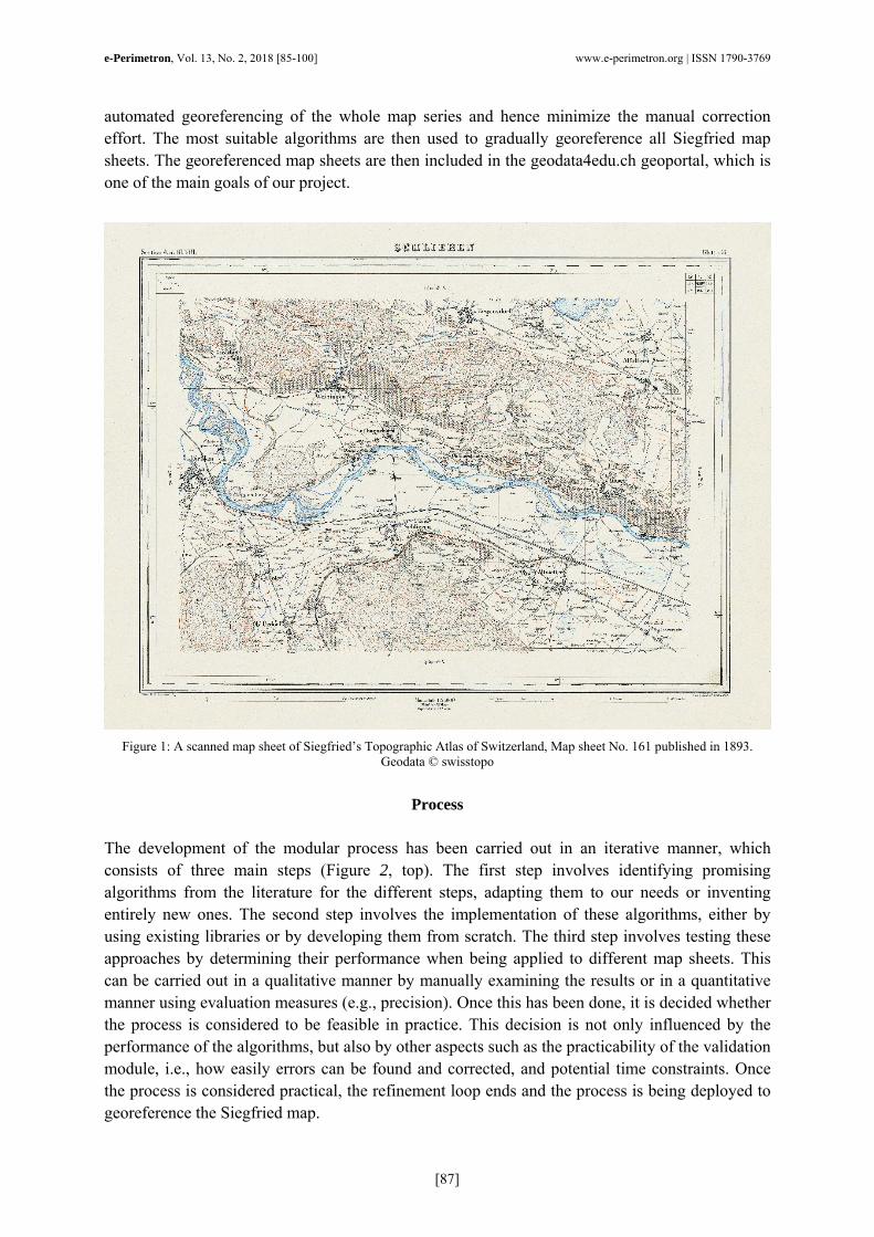
points from the content of the map. Each process has its own advantages. For example, georeferencing the map to its coordinates using the map’s grid, gives the opportunity to compare the content of the map and detect local deformations on it. On the other hand, the use of characteristic points as control points is obligatory, if there is no grid drawn on the map to be used for georeferencing. The procedure followed in both cases is first to find a set of common points, on both the historical map and the reference map (grid intersections or landmarks) and then, to georeference the map using these points as control points. In case the reference system of the historical map is known and there is a grid drawn on it, it is important first to reconstruct the reference system of the map and to generate its grid on the same system that is going to be used for the georeferencing. In this way, the map is properly registered to the grid and it acquires its correct coordinates and its physical dimensions, eliminating deformations derived from the scanning procedure changing the initial size of the map (Tsorlini et al. 2013). The georeferencing procedure is not very complicated, although it can be sometimes challenging, if the number of historical maps to be georeferenced is large. For example, georeferencing a map series consisting of 500 map sheets, even if they have a common known reference system, it is time consuming and it needs a lot of manual effort for every single map sheet. In this case, taking into account the fact that the map sheets have the same reference system, which is well defined, it would be helpful to automatize the procedure, so that the historical maps are correctly georeferenced in a short period of time. In this direction, there are already some approaches, which try to automatize the process of registering a map (Chen et al. 2008; Li et al 2013). The three main steps are: a) to extract a set of reference features from the map that can be used for registering the map, b) to find a set of control point pairs that relate the extracted features with another georeferenced dataset and finally c) to use these points to transform the map to other geospatial data (Chiang et al. 2014). From these steps, the one which is the most difficult to be automated is the detection of the common control points on the map and the georeferenced dataset (Chen et al. 2008; Li et al. 2013; Chiang et al. 2014). This happens mostly due to missing georeference information of the map (projection system and geodetic datum). This process can be more challenging, even if it is done manually, due to the content and the design of historical maps, which in most cases follow different cartographic standards. In this paper, we present a modular process developed in the frame of our project, for automatizing the georeferencing procedure. The Siegfried map series was published from 1870 to 1926 and it has been updated until 1949, though no actual revision cycle is apparent. The map consists of 604 map sheets, which were drawn in the same reference system1 and in two different scales (1:25000 for the Swiss plateau, the French Pre-alps, the Jura Mountains and southern Ticino, and 1:50000 for other mountain regions and the Swiss Alps) (Höhener and Klöti 2010). On every map sheet, there is a grid, which is used to provide the control points for the georeferencing process. An example of a Siegfried map sheet is given in Figure 1. In order to standardize and automatize the whole procedure, different algorithms were investigated in every step of the process to determine those that give better results regarding the 1 The geodetic basis used for this map series was the “Schmidt ellipsoid from 1828” and its fundamental point was the old observatory in Bern. The map is drawn in an equal area, untrue conical projection, known as Bonne projection or as modified Flamsteed projection, using the prime Meridian of Paris. The grid on the map sheets is traced every 1500 meters in the map sheets dated before 1913 and every 1000 meters in those dated after 1917. Source: Hintergrundinformationen zur Siegfriedkarte: https://www.swisstopo.admin.ch/de/wissen-fakten/karten-und-mehr/historische-kartenwerke/siegfriedkarte.html (accessed March, 7th 2018)


[87]

automated georeferencing of the whole map series and hence minimize the manual correction effort. The most suitable algorithms are then used to gradually georeference all Siegfried map sheets. The georeferenced map sheets are then included in the geodata4edu.ch geoportal, which is one of the main goals of our project.

Figure 1: A scanned map sheet of Siegfried’s Topographic Atlas of Switzerland, Map sheet No. 161 published in 1893.

Geodata © swisstopo

Process The development of the modular process has been carried out in an iterative manner, which consists of three main steps (Figure 2, top). The first step involves identifying promising algorithms from the literature for the different steps, adapting them to our needs or inventing entirely new ones. The second step involves the implementation of these algorithms, either by using existing libraries or by developing them from scratch. The third step involves testing these approaches by determining their performance when being applied to different map sheets. This can be carried out in a qualitative manner by manually examining the results or in a quantitative manner using evaluation measures (e.g., precision). Once this has been done, it is decided whether the process is considered to be feasible in practice. This decision is not only influenced by the performance of the algorithms, but also by other aspects such as the practicability of the validation module, i.e., how easily errors can be found and corrected, and potential time constraints. Once the process is considered practical, the refinement loop ends and the process is being deployed to georeference the Siegfried map.


[88]

During these iterations, it turned out that the distinct steps of the georeferencing procedure remained constant in terms of the data to be exchanged between them (Figure 2, bottom). However, the concrete algorithms to be used in this process have been improved or have been entirely exchanged. Hence, we call each of these steps a module with a static interface to other modules but for which different algorithms can be provided.

Figure 2: Development cycle of the georeferencing process (top) and the resulting modules (bottom).

The first module (pre-processing) produces derivations of the original map sheets depending on the requirements of subsequent modules. This may require undertaking any filtering of colour spaces, improving the contrast and lightness, and other properties. The second module (segmentation) subdivides the map into different regions, for example by determining the map frame, the map content and the area in-between. The third module (reference point detection) localizes the grid intersections inside the map content. The fourth module (coordinate extraction) detects the four coordinates between the map content and the map frame, while the fifth module (coordinate interpretation) transforms the detected coordinates into machine-readable form. After the execution of these modules, in the sixth module, the user should validate (validation) the results to ensure that no errors occurred. If there are errors, the user should correct them. Finally, in the seventh module (georeferencing), the extracted data are used to undertake the actual georeferencing.

Modules In this section, the different approaches, which are used within the distinct modules are explained. The focus lies on the approaches used in the most recent realization of the process. However, alternative approaches, which are not used anymore, are also explained, in case when they are considered to be of reader’s interest. They may nonetheless be valuable for other researchers facing similar tasks.

Module 1: Pre-processing

Pre-processing the original image in different ways can significantly improve the performance of the algorithms in other modules or it may be even required for them to function properly. This section describes several of these resulting variations of the original image, which are generated in a sequential manner. In the first step, the contrast and the sharpness of the original map sheet


[89]

(Figure 3A) are adjusted. This removes a large amount of noise and aligns the colours among map sheets (Figure 3B). In particular, the background colour tends to shift towards a plain white. By discarding all coloured pixels from the resulting image, a binary image is obtained (Figure 3C), i.e., an image consisting only of black and white pixels. This representation is useful for many subsequent algorithms, such as the bi-directional histograms and the pattern matching approaches. Finally, the binary image is processed to support the reconstruction of grid lines. This mainly includes the removal of small objects by applying several morphological operations (e.g., erosion and dilation), the Canny algorithm to detect edges and the use of two convolution matrices (Figure 3D) to emphasize horizontal and vertical lines. The result of this process is depicted in Figure 3E.

Figure 3: Steps during preprocessing. A: Original image. B: Color-adjusted image. C: Binary image. D: Filter kernels. E:

Filtered image for grid detection. Geodata © swisstopo

Module 2: Segmentation

Clearly delineating different regions of the input image is the main purpose of segmentation. It turned out that the most important task for this purpose is to detect the corners of the map frame in order to separate the map content from the remaining image. This is critical, because grid reconstruction algorithms tend to confuse the frame with the grid lines. We describe two ways of how this can be carried out.

Template-Matching Probably the most straight-forward approach to detect key features of a map sheet is to reconstruct its different areas based on template-matching. This is performed by making use of a moving window approach during which the content of each window is compared against a template. The object is then found when the difference between the template and the content of the window is the lowest. In practice, it turned out that this approach is hardly generically applicable out-of-the box. Even the detection of corners is difficult because their appearance may change among map sheets and often similar patterns can be found within the map content. To work around this issue, the templates were applied on a modified input image. It proved useful, for example, to apply erosion operations on the binary image depicted in Figure 3C to unify the appearance of the corners and to subsequently create a template based on them. This way, one template can be used for several map sheets.

Bi-directional histograms The bi-directional histogram approach was implemented as a first idea to partition the map sheet. The way it works is explained in Figure 4 using an idealized example. The original situation is depicted in Figure 4A. It shows a schematized binary image that originally contained a rectangle with a black outline. The pixels, which were part of the outline are indicated by dashed red lines. The image, however, contains noise, making a direct extraction of this rectangle cumbersome.


[90]

Computing a bi-directional histogram makes this task easier. This is performed as follows. First, for each row and each column, the number of white pixels is counted (see numbers at the borders in Figure 4A). The resulting numbers are added up for each pixel considering the pixel counts of the row and the column it belongs to. Applying a threshold to the result yields another binary image (Figure 4B). In this simple example, a threshold of 8 was used, converting all values above this number to white pixels and all values below or equal to black pixels. Repeating the process allows to identify the corners of the original image. These are indicated by the pixels whose bi-directional sum is zero (Figure 4C). Figure 5 depicts three iterations of this process applied to the binary image of a Siegfried map sheet. After two iterations (Figure 5B), the three main areas can be clearly distinguished. The central black area shows the map content, the white areas show the corners and the grey areas show the remaining parts, which contain the map coordinates.

Figure 4: Concept of the bi-directional histogram.

This approach only works well when dealing with features that cover the horizontal and vertical axes of the map sheet. Rotated crosses, for example, cannot be detected in this manner. In addition, it may not be obvious to pick suitable threshold values to clearly separate the areas from each other. The approach, however, proved to be useful for the purpose of detecting corners on the Siegfried map on some map sheets. Ultimately, it was discarded because template-matching was easier to be applied and does not require estimating the threshold parameter.

Figure 5: Three cycles of computing and thresholding bi-directional histograms.

A: One iteration. B: Two iterations. C: Three iterations.


[91]

Module 3: Reference point detection

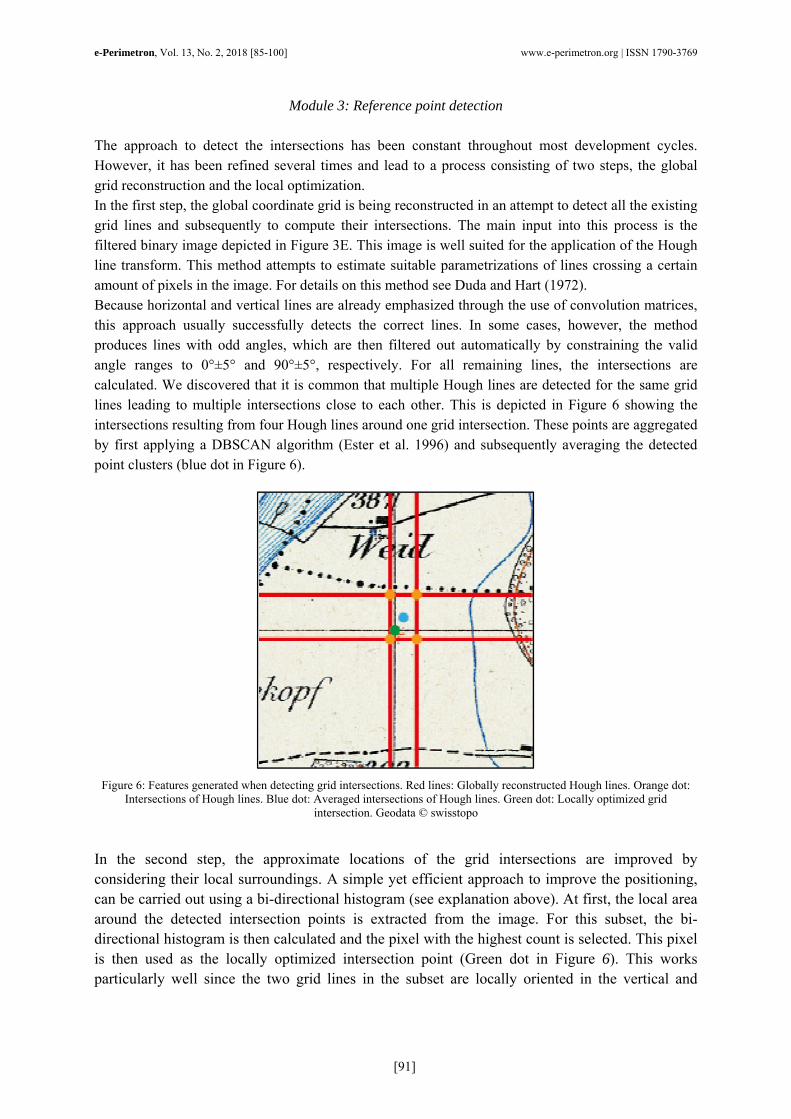
The approach to detect the intersections has been constant throughout most development cycles. However, it has been refined several times and lead to a process consisting of two steps, the global grid reconstruction and the local optimization. In the first step, the global coordinate grid is being reconstructed in an attempt to detect all the existing grid lines and subsequently to compute their intersections. The main input into this process is the filtered binary image depicted in Figure 3E. This image is well suited for the application of the Hough line transform. This method attempts to estimate suitable parametrizations of lines crossing a certain amount of pixels in the image. For details on this method see Duda and Hart (1972). Because horizontal and vertical lines are already emphasized through the use of convolution matrices, this approach usually successfully detects the correct lines. In some cases, however, the method produces lines with odd angles, which are then filtered out automatically by constraining the valid angle ranges to 0°±5° and 90°±5°, respectively. For all remaining lines, the intersections are calculated. We discovered that it is common that multiple Hough lines are detected for the same grid lines leading to multiple intersections close to each other. This is depicted in Figure 6 showing the intersections resulting from four Hough lines around one grid intersection. These points are aggregated by first applying a DBSCAN algorithm (Ester et al. 1996) and subsequently averaging the detected point clusters (blue dot in Figure 6).

Figure 6: Features generated when detecting grid intersections. Red lines: Globally reconstructed Hough lines. Orange dot:

Intersections of Hough lines. Blue dot: Averaged intersections of Hough lines. Green dot: Locally optimized grid intersection. Geodata © swisstopo

In the second step, the approximate locations of the grid intersections are improved by considering their local surroundings. A simple yet efficient approach to improve the positioning, can be carried out using a bi-directional histogram (see explanation above). At first, the local area around the detected intersection points is extracted from the image. For this subset, the bi-directional histogram is then calculated and the pixel with the highest count is selected. This pixel is then used as the locally optimized intersection point (Green dot in Figure 6). This works particularly well since the two grid lines in the subset are locally oriented in the vertical and


[92]

horizontal directions. Globally, this approach does not work well because the grid lines are typically distorted across large distances.

Module 4: Coordinate extraction

Extracting the coordinates requires distinguishing them from similar features on the map. For this purpose, two approaches were investigated; the first one is using a Convolutional Neural Network (CNN) and the second one using template matching. Both methods are applied to all four regions between the map content and the map frame.

Convolutional neural network CNNs have shown impressive results in similar image recognition tasks (Krizhevsky et al. 2012). Hence, it was considered worthwhile to investigate their usefulness for coordinates extraction. At first, 5.0% of all existing Siegfried map sheets were randomly picked and the regions depicting the coordinates were manually labelled. This resulted in 816 coordinate regions. To provide enough negative examples, in total 1632 regions were randomly extracted around the coordinate regions and the map content. The resulting dataset was split into a training set containing 70.0% of the samples and a test set containing 30.0% of the samples. Such a ratio is common for comparable machine learning tasks and can be found, for example, in remote sensing applications as described by Rogan et al. (2008). However, it can be worthwhile to investigate different sampling schemes. The CNN used consists of three convolutional layers and a fully connected layer with several max pooling (Ranzato et al. 2007) layers in-between. The network achieves an accuracy of 99.1% on the training set and 98.1% on the test set. In practice, the network is applied to each area where the coordinates are supposed to be placed using a moving window approach. In this setting, it still has issues distinguishing between coordinates and labels as exemplified in Figure 7.

Figure 7: Coordinate candidates detected by the Convolutional Neural Network. Geodata © swisstopo

To overcome the issue of false positives detected by the CNN, a mechanism has been included to select the most probable coordinate region from a set of candidates. For this purpose, each candidate region is passed to the coordinate interpretation module to recognize the distinct symbols. The results are returned to the coordinate extraction module and evaluated using several logical tests. They include, for example, methods to validate the number of coordinates (e.g., a total of three digits is not possible) and the orientation (e.g., the left and right orientation must be either “O”, “E” or “W”). Finally, the region, which passes the majority of these tests is selected as the actual coordinates and the resulting coordinates are forwarded to subsequent modules.


[93]

Template-Matching One common characteristic of the coordinates is their structure. Usually, there are up to six coordinate numbers, followed by a unit sign (an elevated “m” with a dot below it) and a letter in the end indicating the orientation of the coordinates (see Figure 7). In a first approach, a template was used to detect the characteristic “m” symbol and to extract the regions left and right of it to be interpreted. This approach, however, has several limitations. At first, the “m” symbol itself comes in several fonts and sizes, depending on the map sheet. Secondly, the dot is sometimes irregularly placed or may even be missing entirely. Thirdly, if an “m” as part of a label is placed above other features, such as small buildings, the method yields false positives. Hence, this approach was not considered robust enough to be further investigated.

Module 5: Coordinate interpretation Converting coordinates detected by the coordinate extraction module requires delineating the distinct symbols and interpreting their meaning. This results in a set of characters understandable by computers. For this purpose, the use of convolutional neural networks and of an out-of-the-box software, tesseract, have been investigated.

Convolutional neural networks Inspired by the good performance of the CNN used for coordinate extraction, another CNN for categorizing the distinct symbols has been set up. For this purpose, the manually extracted coordinates described earlier have been split into the distinct symbols. They have been manually labeled resulting in a dataset of 9562 single symbols. These were again split into a training set consisting of 70.0% of the samples and a test set consisting of 30.0% of the samples. The CNN consists of two convolutional layers followed by two densely connected layers with several max-pooling and dropout (Srivastava et al. 2014) layers in-between. The CNN achieves an accuracy of 99.7% on the training set and 99.3% on the test set. The main issue when applying the CNN, however, is related to the separation of the distinct symbols from the extracted coordinate images. A straightforward approach for this purpose is to extract rectangular regions from the image based on the bounding box of each connected component. This, however, performs well only when all pixels making up a symbol are completely connected; it is not working when two symbols touch each other or additional features interfere with any symbol. To tackle this issue, several heuristics have been implemented in an attempt to improve the segmentation of the coordinates. For example, distinct components with overlapping bounding boxes are passed to the CNN as a single component. In addition, zeroes are often split into two crescent-shaped components due to their poor graphical quality. When two such crescents are encountered, they are likewise treated as a common symbol and the respective bounding box is passed to the CNN for interpretation.

Tesseract As a first attempt, tesseract2, a freely available optical character recognition (OCR) tool was used to analyse the coordinates. The application of the software did not yield satisfying results as nearly no symbol was correctly interpreted. No fundamental improvements could be achieved by pre-processing the coordinates (e.g., de-noising, up-sampling) or by limiting the symbols to be

2 Tesseract OCR: https://opensource.google.com/projects/tesseract (accessed February, 28th 2018)


[94]

detected to numbers and the valid directions (“N”, “S”, “W”, “E”, “O”). The low performance can presumably be attributed to the low quality of the input images, the varying relative positioning of the distinct symbols and the unconventional fonts used in the Siegfried map. An option to improve the results of tesseract would be to specifically train it on the target fonts, which has not been done in this study. Nonetheless, tesseract can be used out-of-the-box and hence may serve as a first approach when dealing with historical maps depicting coordinates in a better graphical quality.

Module 6: Validation It is crucial to provide a convenient way to analyse the results of the algorithms described earlier. For this purpose, a QGIS-file is generated for each processed map sheet. By default, it displays the cropped map sheet, the locations of the detected intersections and the interpreted coordinates (Figure 8). The user can thus easily examine these results and may correct them if required by using the editing functionality of QGIS. These changes are then accounted for by the final georeferencing module.

Figure 8: QGIS-project depicting the results of the automatic analysis process. Geodata © swisstopo


[95]

Module 7: Georeferencing

Once the intersection points have been correctly localised and the coordinates have been correctly interpreted, the actual georeferencing step can be performed. This requires defining the target raster (extent, resolution) and subsequently determining the pixel colour for each the raster’s cells. Finally, this raster needs to be transformed to a known Coordinate Reference System (CRS) to be usable in GIS environments.

Quadrilateral-based bi-linear interpolation In a scanned Siegfried map sheet each pixel of the map content is placed inside a distorted quadrilateral formed by four intersection points. The location of these intersection points within the target raster is exactly defined by the coordinates of the coordinate grid. Hence, the first step in georeferencing the sheet is to realign these distorted quadrilaterals to their original form, meaning rectangles whose edges are placed in parallel. A pixel of the newly created rectangle is then interpolated based on the original locations of the intersections in the untransformed map sheet. This is being carried out using quadrilateral-based interpolation. The first step requires determining the coordinates at each intersection point. For the outermost points, the coordinates are directly given by the coordinates derived from the coordinate interpretation module. For the remaining, interior, points the coordinates are linearly interpolated and rounded to the nearest multiple of 250m. This number represents the minimum distance between two grid lines discovered in the Siegfried map.

Figure 9: Schematized interpolation process to determine pixel colors of the final Siegfried map sheet. A: Layout of the target

raster with rectangles indicating the different cells formed by the projected coordinate grid. B: Raster of a single projection grid cell. The coordinates of each raster cell are given in a local normalized coordinate system. C: The same projection grid cell as in B, but distorted as depicted on the Siegfried map. The corner points are given in pixel coordinates of the original

image. Figure partially derived from particleincell.com (2012).

In the second step, the target raster is defined (Figure 9A). The dimensions of this raster are calculated by dividing the width and height in meters by the target resolution r (e.g., 1.25 meters per pixel). The width is given by subtracting the west coordinate CW from the east coordinate CE. The height correspondingly is obtained by subtracting the southern coordinate CS from the northern coordinate CN. This raster is then split into the rectangles defined by the coordinates of the corners of the projection grid cells. Figure 9B displays one of the central projection grid cells. The projection grid cell consists of raster cells, which are indexed by the normalized coordinates j and i, each being in the range [0, 1]. To determine the color of each raster cell, its normalized coordinates are used to calculate the raster cell’s location in the corresponding distorted projection grid cell of the scanned Siegfried map sheet (Figure 9C) using the method described by particleincell.com (2012).


[96]

This location is defined in terms of the global image coordinate system spanned by the axes x and y. The mapping from (i, j) to (x, y) can be carried out using the formulas below.

+ +

The coefficients α and β can be derived based on the corner points of the distorted quadrilateral. A detailed explanation of how these parameters can be obtained is given by particleincell.com (2012). Once the respective image coordinates (x, y) are calculated, a nearest neighbour interpolation is applied to determine the value to be stored at (i, j). Finally, the coordinates are transformed to the modern coordinate reference system (CRS) of Switzerland, LV95. This is done by assuming that the grids of the historical CRS and the modern CRS coincide. Hence, the transformation between the two CRS only accounts for the different values for False Easting and False Northing. We are aware that this is only an approximation and are evaluating other ways to improve the transformation. The resulting rasters are stored as GeoTIFF files and can be used in GIS environments. In our case, these files will be integrated into a geoportal to make them accessible to a wide range of users.

Integration into a Geoportal

Geodata are needed in many scientific fields such as environmental management, architecture, urban and landscape planning, or medicine (geodata4edu.ch 2018). Historical geodata in particular allow for the investigation of topographic features over time, which is of great interest to many researchers. To facilitate the access of such data to the scientific community (scientific staff, students), it is aimed to integrate the georeferenced Siegfried map sheets into the “Geodata Versatile Information Transfer environment” (GeoVITe). GeoVITe is the geoportal of the corporate academic spatial data infrastructure of ETH Zurich. The geoportal was initiated to meet the demand for geodata in various academic disciplines of Swiss academia and is a major part of a comprehensive national service offered by geodata4edu.ch (Iosifescu Enescu et al. 2017). GeoVITe offers a user-friendly web interface (Figure 10), where the guiding functional requirements are related to the access, visualization and download of geospatial datasets. A user should be able to visually navigate the available data (spatially, thematically, and temporally), select the desired dataset and area of interest, and be able to directly download the required data (Iosifescu-Enescu et al. 2017).


[97]

Figure 10: Example visualization of the Siegfried map in the GeoVITe web interface. Geodata © swisstopo

Due to the high demand and the significant number of potential users (currently more than 1000 unique users/month), the integration of the georeferenced Siegfried map sheets into the geodata4edu.ch has been defined from the very beginning as one of the main goals of this project. This integration has started recently in 2018, while more datasets are added to the geoportal on a regular basis.

Discussion

The process presented in this paper allows to improve the accuracy in respect to existing georeferencing approaches such as those undertaken by Swisstopo3. Figure 11 depicts the results of both approaches for a small area spanning two adjacent map sheets. On the left, the georeferencing result by Swisstopo is depicted, showing a topological error of a stream spanning two map sheets (Figure 11A). On the right, this error is not present anymore due to the improved georeferencing procedure described in this article. However, another topological error remains for a road in both versions (Figure 11B). Such issues cannot be corrected by further improving the georeferencing process, but necessitate the use of complementary methods such as conflation techniques.

Figure 11: Left: Two adjacent map sheets georeferenced by Swisstopo. Right: The same map sheets georeferenced using the

method described in this paper. Note the corrected topological error at A and the nonetheless mismatching road at B. Geodata © swisstopo

3 Results of their process can be found through the layer “Journey through time – Maps” at https://map.geo.admin.ch/ (accessed February, 28th 2018)


[98]

Obtaining such results is only possible when the coordinate information and the intersection points are correctly determined. To assess how much manual correction (module 6) is required, the modules 1 to 5 have been applied to 20 randomly selected Siegfried map sheets. Since module 1 only performs mainly conventional image-processing tasks, the discussion will focus on modules 2 to 5. For evaluation, precision is used, which is defined as “a ratio of true positives (TP) and the total number of positives predicted by a model” (Ting 2010). Module 2 (image segmentation) has correctly detected all 80 corners and hence achieved a precision of 100.0%. The proposed template-based approach is therefore considered robust enough for corner detection. Module 3 (reference point detection) successfully detected 1097 of a total of 1121 intersection points (precision of 97.9%). Grid points were missed when the coordinate grid is of poor graphical quality or strongly distorted. Of these correctly detected points, another 36 have been wrongly placed in the local optimization phase, leading to an overall precision of 94.6%. This is predominantly the case when map features intersect with grid lines. When computing the bi-directional histogram, this leads to a shift of the maximum count away from the actual intersection. Module 4 (coordinate detection) successfully detected 75 of the 80 coordinates (precision of 93.8%). In each of these cases, the actual coordinates were part of the candidates, but have been ultimately discarded in favour of other candidates. Most of these mistakenly chosen candidates contain meaningless text. This demands for adding more logical tests. Module 5 (coordinate interpretation) correctly interpreted 460 of the 481 coordinate symbols (precision of 95.6%). This includes errors due to symbols being mistakenly discarded, interpreted incorrectly, or elements not being part of the coordinates being interpreted. The average processing time of one map sheet amounted to 80.4 seconds. The processing times for module 1, 2 and 3 amounted to 2.5 seconds, 8.6 seconds and 2.7 seconds, respectively. The interconnected modules 4 and 5 amounted to the remaining 66.7 seconds and hence are by far the most time-consuming modules. To successfully georeference a map sheet, all coordinates need to be correctly detected and interpreted, since a single mistake (e.g., missing a zero) may considerably misplace the sheet. In addition, it is critical to at least detect all outermost intersection points. Not doing so leads to high distortions in the resulting georeferenced image and regions at the boundary being discarded entirely. Missing points within the map sheet and displaced intersection points are not as critical since the resulting distortions are smaller. However, these mistakes, too, need to be avoided, when high accuracies need to be achieved. In only two map sheets (10.0%) have the modules 1 to 5 resulted in perfect results making it possible to perform the georeferencing without any manual adjustment. In another six map sheets (30.0%) all coordinates have been correctly detected and interpreted, but some intersection points have been displaced, leading to local inaccuracies in the georeferenced raster. In the remaining 60.0% of the map sheets, either some coordinates have not been detected/interpreted correctly and/or some intersection points at the borders of the map content have been missed. Hence, the underlying challenge when creating an automatic georeferencing system lies in the combined probabilities of the single modules to successfully perform the georeferencing task. Although the single precisions of the discussed modules are high (>90.0%), their combined application may lead to very low success rates. Let us consider module 5 (coordinate interpretation) to demonstrate this issue. Assuming four coordinates each consisting of six symbols and a probability of 95.6% to correctly interpret each of them leads to an overall probability of 0.95624 = 0.34 = 34%. Therefore, only in the case of every third map sheet will all


[99]

coordinates be correctly interpreted. When additionally considering the performance of other modules, this percentage drops even further. We only see two ways to tackle this issue. First, by improving the performance of the single modules and, second, by making the manual validation phase more convenient. The latter may involve developing further logical tests that help in highlighting potential errors or by using software packages tailored to labelling and validating such results (e.g., using the VGG Image Annotator4). Nonetheless, it is aimed to use the most recent implementation of the described workflow to carry out the georeferencing of the whole Siegfried map series. It is expected that this still requires considerable manual effort to compensate for the issues described above.

References

Chen C.-C., C. A. Knoblock, C. Shahabi (2008). Automatically and accurately conflating raster maps with orthoimagery. GeoInformatica 12 (3): 377–410. In digital form: https://link.springer.com/article/10.1007/s10707-007-0033-0

Chiang YY., Leyk S., Knoblock C.A. (2014). A Survey of Digital Map Processing Techniques. ACM Computing Surveys, 47 (1): Article 1. In digital form: http://dl.acm.org/citation.cfm?id=2557423

Duda, R. O., & Hart, P. E. (1972). Use of the Hough transformation to detect lines and curves in pictures. Communications of the ACM, 15(1), 11-15, doi:10.1145/361237.361242.

Ester, M., Kriegel, H.-P., Sander, J., & Xu, X. (1996). A density-based algorithm for discovering clusters in large spatial databases with noise. In Proceedings of the Second International Conference on Knowledge Discovery and Data Mining, Portland, Oregon.

geodata4edu.ch. (2018). Possible fields of application. In digital form: https://www.geodata4edu.ch/en/service/possible-fields-of-application/. Last accessed February, 2nd 2018.

Höhener H.-P., P. Klöti (2010). Geschichte der schweizerischen Kartographie. Kartographische Sammlungen in der Schweiz, Bern. In digital form: http://boris.unibe.ch/57737/1/2010_Hoehener_a.pdf

Iosifescu Enescu, I., Gkonos, C., Iosifescu Enescu, C. M., Tsorlini, A., Hotea, M., Piguet, A., & Hurni, L. (2017). In Proceedings of the 28th International Cartographic Conference, Washington DC, USA. Guidelines for a Comprehensive Design of Geoportals based on Open Geospatial Software.

Iosifescu-Enescu, I., Matthys, C., Gkonos, C., Iosifescu-Enescu, C. M., & Hurni, L. (2017). Cloud-Based Architectures for Auto-Scalable Web Geoportals towards the Cloudification of the GeoVITe Swiss Academic Geoportal. ISPRS International Journal of Geo-Information, 6(7): 192. doi: 10.3390/ijgi6070192

Krizhevsky, A., Sutskever, I., & Hinton, G. E. (2012). ImageNet classification with deep convolutional neural networks. In Proceedings of the 25th Conference on Advances in Neural Information Processing Systems, 1097-1105. In digital form: https://papers.nips.cc/paper/4824-imagenet-classification-with-deep-convolutional-neural-networks.pdf.

Li. Y., R. Briggs (2013). An automated system for image-to-vector georeferencing. Cartography and Geographic Information Science, 39 (4): 199-217. In digital form: http://www.tandfonline.com/doi/abs/10.1559/152304063941199.

4 VGG Image Annotator: http://www.robots.ox.ac.uk/~vgg/software/via/ (accessed February, 28th 2018)


[100]

particleincell.com (2012). Interpolation using an arbitrary quadrilateral. In digital form: https://www.particleincell.com/2012/quad-interpolation/. Last accessed February, 2nd 2018.

Ranzato, M., Huang, F. J., Boureau, Y. L., & LeCun, Y. (2007). Unsupervised Learning of Invariant Feature Hierarchies with Applications to Object Recognition. In Proceedings of the 2007 IEEE Conference on Computer Vision and Pattern Recognition, Minneapolis, USA. doi:10.1109/CVPR.2007.383157.

Rogan, J., Franklin, J., Stow, D., Miller, J., Woodcock, C., & Roberts, D. (2008). Mapping land-cover modifications over large areas: A comparison of machine learning algorithms. Remote Sensing of Environment, 112 (5): 2272-2283. doi:10.1016/j.rse.2007.10.004.

Srivastava, N., Hinton, G., Krizhevsky, A., Sutskever, I., & Salakhutdinov, R. (2014). Dropout: a simple way to prevent neural networks from overfitting. Journal of Machine Learning Research, 15 (1):1929-1958. In digital form: http://jmlr.org/papers/volume15/srivastava14a/srivastava14a.pdf.

Ting, K. M. (2010). Precision. In C. Sammut, & G. I. Webb (Eds.), Encyclopedia of Machine Learning, 780. Boston, MA: Springer US.

Tsorlini A., I. Iosifescu, L. Hurni (2013). Comparative analysis of historical maps of the Canton of Zurich - Switzerland in an interactive online platform. In Proceedings of the 26th International Cartographic Conference, Dresden, Germany. In digital form: http://icaci.org/files/documents/ICC_proceedings/ICC2013/_extendedAbstract/147_proceeding.pdf.

Tsorlini A., Hurni L. (2015). On the georeference and re-projection of old maps in different application software: comparing methodology and results. In Proceedings of the 10th Jubilee Commission Conference on Digital Approaches to Cartographic Heritage, Corfu, Greece.

keywords: siegfried map, georeferencing, image-processing

Documents