A new algorithm for improveddeterminant computation with a view

towards resultantsby

Khalil Shivji

Thesis Submitted in Partial Fulfillment of theRequirements for the Degree ofHonours Bachelor of Science

in theDepartment of Mathematics

Faculty of Science

c© Khalil Shivji 2019SIMON FRASER UNIVERSITY

Fall 2019

Copyright in this work rests with the author. Please ensure that any reproductionor re-use is done in accordance with the relevant national copyright legislation.

Approval

Name: Khalil Shivji

Degree: Honours Bachelor of Science (Mathematics)

Title: A new algorithm for improved determinantcomputation with a view towards resultants

Supervisory Committee: Dr. Michael MonaganSupervisorProfessor of Mathematics

Dr. Nathan IltenCourse InstructorAssociate Professor of Mathematics

Date Approved: December 13, 2019

ii

Abstract

Certain symbolic matrices can be highly structured, with the possibility of having a blocktriangular form. Correctly identifying the block triangular form of such a matrix can greatlyincrease the efficiency of computing its determinant. Current techniques to compute theblock diagonal form of a matrix rely on existing algorithms from graph theory which do nottake into consideration key properties of the matrix itself. We developed a simple algorithmthat computes the block triangular form of a matrix using basic linear algebra and graphtheory techniques. We designed and implemented an algorithm that uses the Matrix Deter-minant Lemma to exploit the nature of block triangular matrices. Using this new algorithm,the computation of any determinant that has a block triangular form can be expedited withnegligible overhead.

Keywords: Linear Algebra; Determinants; Matrix Determinant Lemma; Schwartz-ZippelLemma; Algorithms; Dixon Resultants

iii

Dedication

For my brothers,Kassim, Yaseen, and Hakeem.

iv

Acknowledgements

I would like to acknowledge Dr. Michael Monagan for providing his support throughout theentire research project. This project would not have been possible without his commitmenttowards developing whatever was needed to move forwards. Additionally, I would like tothank Dr. Nathan Ilten for taking the time to create a rewarding research course, and forgiving us some insight as to what it is like to be a mathematician. I would also like to thankDavid Sun, who began this research project with me and someone who positively influencedmany ideas throughout the project. Lastly, I would like to acknowledge NSERC and SimonFraser University for giving me the special opportunity to participate in research.

v

Table of Contents

Approval ii

Abstract iii

Dedication iv

Acknowledgements v

Table of Contents vi

List of Tables viii

List of Figures ix

1 Introduction 11.1 History . . . . . . . . . . . . . . . . . . . . . . . . . . . . . . . . . . . . . . 11.2 Resultants . . . . . . . . . . . . . . . . . . . . . . . . . . . . . . . . . . . . . 21.3 Structured matrices . . . . . . . . . . . . . . . . . . . . . . . . . . . . . . . 3

2 Tools, Methods, & Vocabulary 52.1 Notation . . . . . . . . . . . . . . . . . . . . . . . . . . . . . . . . . . . . . . 52.2 Motivation for Dixon’s Method . . . . . . . . . . . . . . . . . . . . . . . . . 62.3 Dixon’s method . . . . . . . . . . . . . . . . . . . . . . . . . . . . . . . . . . 72.4 The area of a triangle . . . . . . . . . . . . . . . . . . . . . . . . . . . . . . 12

3 Determinants 153.1 An overview of methods . . . . . . . . . . . . . . . . . . . . . . . . . . . . . 153.2 Minor expansion by Gentleman & Johnson . . . . . . . . . . . . . . . . . . 153.3 Characteristic polynomials by Berkowitz . . . . . . . . . . . . . . . . . . . . 173.4 A comparison of methods . . . . . . . . . . . . . . . . . . . . . . . . . . . . 18

4 Algorithms for revealing block structure 204.1 Divide and Conquer . . . . . . . . . . . . . . . . . . . . . . . . . . . . . . . 204.2 Phase 2: Link . . . . . . . . . . . . . . . . . . . . . . . . . . . . . . . . . . . 21

vi

4.3 Phase 1: Clarify . . . . . . . . . . . . . . . . . . . . . . . . . . . . . . . . . . 254.3.1 Upper block triangular matrices . . . . . . . . . . . . . . . . . . . . 254.3.2 Explanation and proof for Clarify algorithm . . . . . . . . . . . . . . 27

5 Empirical Results 30

6 Conclusion 33

Bibliography 35

Appendix A Code 37

vii

List of Tables

Table 2.1 Elimination techniques 1 . . . . . . . . . . . . . . . . . . . . . . . . . 7Table 2.2 Elimination techniques 2 . . . . . . . . . . . . . . . . . . . . . . . . . 7

Table 3.1 Numerical determinant computation methods . . . . . . . . . . . . . . 18Table 3.2 Symbolic determinant computation methods . . . . . . . . . . . . . . 19

Table 5.1 Systems information for Dixon matrices . . . . . . . . . . . . . . . . . 31Table 5.2 Block structure and multiplication count . . . . . . . . . . . . . . . . 32

viii

List of Figures

Figure 2.1 Heron’s problem . . . . . . . . . . . . . . . . . . . . . . . . . . . . . 12

Figure 3.1 Code for random symbolic matrices . . . . . . . . . . . . . . . . . . 19

Figure 4.1 Plot of speedup from computing block diagonal form of A′ . . . . . 22Figure 4.2 Transforming a matrix into block diagonal form . . . . . . . . . . . 22

ix

Chapter 1

Introduction

1.1 History

From robotics [CLO15, chapter 3] to geodesy [PZAG08], to control theory [Pal13], systemsof polynomial equations have the power to model complex problems. A solution of a systemof polynomial equations might identify the optimal placement of an antenna on a satellite.It could help robots navigate through space more effectively, giving rise to machines morecapable then ever before. These polynomial systems, and the methods for solving them,have helped realize countless modern advances across a variety of domains.

Elimination theory is concerned with developing methods and techniques for solvingsystems of polynomial equations. These techniques revolve around the idea that we cangenerate new polynomial equations from a given collection of polynomials that involvefewer variables. Under certain circumstances which will be discussed later on, the solutionsets of these new polynomials give us a hint as to what the solution to the original systemlooks like.

Definition 1.1.1. [GCL92, chapter 9] A solution (or root) of a system of j polynomialequations in r variables

pi(x1, x2, . . . , xr) = 0, 1 ≤ i ≤ j. (1.1)

over a field k is an r-tuple (α1, α2, . . . , αr) from a suitably chosen extension field of k suchthat

pi(α1, α2, . . . , αr) = 0, 1 ≤ i ≤ j. (1.2)

Given a large system of equations in many variables, it will most likely be difficult tosee what the solution could be just by inspection. The general idea of elimination theoryis to eliminate variables from a system of polynomial equations to produce new equationsin a subset of the original variables. The advantage is that these new equations have fewervariables, which provides us with the opportuniyt to find a partial solution. Given thatcertain properties hold, these partial solutions can then be extended to full solutions as wehave described them in Definition 1.1.1.

1

When considering linear equations, a solution can be obtained using the combination ofGaussian elimination and back substitution. Systems of equations that are row equivalentshare the same solution set [Lay06]. Reducing the system to row echelon form generatesnew polynomials from the lower rows that have fewer variables. From this point of view, itis easier to see a potential solution or lack thereof.

Gaussian Elimination provides us with a method of systematically eliminating variablesfrom a system of linear equations. What about systems of polynomials that contain non-linear equations?

Throughout the 19th and 20th century mathematicians such as Sylvester [Has07, chapter5] and Macaulay [Mac03] improved our understanding of solutions sets of polynomial sys-tems, and produced general methods for obtaining solution sets to multivariate non-linearsystems. They developed methods to produce what are known as eliminants. These areobjects, often polynomials, that would give them an indication of whether such a solutionexists. These eliminants include the familiar quadratic discriminant b2− 4ac, which tells uswhether the polynomial ax2 + bx + c has any real solutions, and whether it has a doubleroot.

In 1965, Bruno Buchburger introduced his algorithm for computing a Gröbner ba-sis [Buc76]. Once a Gröbner basis of an ideal defined by a collection of polynomials hasbeen computed, one can more easily answer many questions related to the existence of so-lutions, and how to generate them. It is one of the main tools used in elimination theorytoday, as computer algebra systems have become powerful enough to handle relatively largesystems. Buchburger’s algorithm can be seen as a non-linear analogue of Gaussian elimi-nation, so it is not hard to believe that it can help us uncover the solution to a system ofpolynomial equations [CLO15].

1.2 Resultants

We would like to preface this discussion on resultants by saying that it is not the purposeof this thesis to give a complete and rigorous treatment of resultant theory. We wish toprovide a basic introduction to the ideas and techniques that we found helpful in computingresultants. This will provide some motivation as to why computing resultants is important.

We begin by providing the most general definition of a resultant. While this definitionmay seem abstract, its power lies in its generality. While we will not discuss all typesof resultants, this definition has allowed mathematicians such as Sylvester [CLO15] andMacaulay [Mac03] to formulate resultants in different contexts.

Definition 1.2.1. [GKZ94, Chapter 12] The resultant of k+1 polynomials f0, f1, . . . , fk ink variables is defined as an irreducible polynomial in the coefficients of f0, f1, . . . , fk, whichvanishes whenever these polynomials have a common root.

2

In 1908, Dixon defined a sequence of steps that allows us to eliminate one variable froma system of two polynomial equation [Dix08]. One year later, he published a similar paperdescribing a procedure to eliminate two variables from three equations [Dix09]. Almost acentury later in 1994, Kapur, Saxena, and Yang generalized Dixon’s method for systems Fof n + 1 polynomial equations with n variables [KSY94]. Their idea, known as the KSY-variant of Dixon’s method, eliminates n variables, leaving us with a polynomial in thecoefficients of F . This polynomial is known as the Dixon resultant. Dixon’s method uses amatrix called Dixon’s matrix, a matrix whose determinant produces a Dixon resultant. It issimilar in many respects to other matrix-based resultant formulations such as the Bèzout’smatrix [Cay57] and Sylvester’s matrix. Because the Dixon’s method relies on determinantcomputations, its time complexity is more manageable than that of Buchburger’s algorithm.This is not to say computing symbolic determinants is always fast enough for practicalapplications. We require a plethora of tools and tricks to compute symbolic determinantsefficiently, some of which we will see in chapters 3 and 4.

1.3 Structured matrices

It is possible to formulate many geometric problems as systems of polynomial equations.Computing the Dixon resultant for such systems can provide us with information aboutthe solution to these system. Viewed in the correct context, the solution of such a systemcan give us information about the volume of tetrahedron [KSY94], or prove geometric the-orems [Kap97],[CLO15, Chapter 6]. Although it has not yet been detailed in the literature,the Dixon matrix of systems of polynomial equations that represent geometric problem areoften highly structured. This is most likely due to some underlying structure of the polyno-mials. These Dixon matrices frequently present themselves as row and column permutationsof block triangular matrices. These matrices have what is known as a block triangular form.However, these matrices can be quite large, so determining if a matrix has a block triangularform is no trivial task. A large portion of our research went into developing an algorithmthat is able to detect this structure within matrices.

If a matrix has a block triangular form, then many matrix computations become easierto perform. Most importantly for us, the determinant of a block triangular matrix is theproduct of the determinants of each sub-matrix along the main diagonal [Dym13]. Sinceeach one of these sub-matrices is smaller, we can more efficiently compute the determinantof large matrices by splitting the problem into many smaller determinant computations.This is especially true if the matrix is a symbolic one, that is to say, it has polynomialsin its entries. Dixon matrices are symbolic matrices that can have a block triangular form.Determinant computations can become infeasible if this block structure is not exploited.The challenge is that it is not trivial to compute a block triangular form, even if we know

3

a priori the matrix has one. Therefore it is crucial that we have an efficient method fordetecting and computing block triangular forms in matrices.

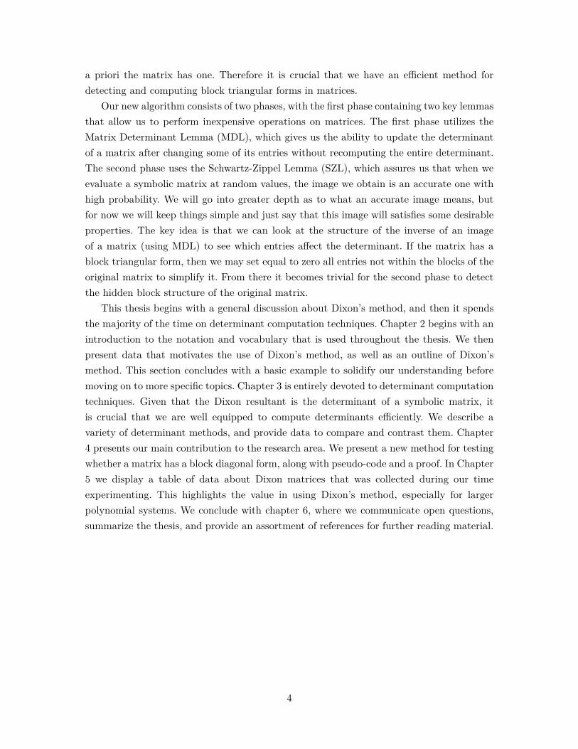
Our new algorithm consists of two phases, with the first phase containing two key lemmasthat allow us to perform inexpensive operations on matrices. The first phase utilizes theMatrix Determinant Lemma (MDL), which gives us the ability to update the determinantof a matrix after changing some of its entries without recomputing the entire determinant.The second phase uses the Schwartz-Zippel Lemma (SZL), which assures us that when weevaluate a symbolic matrix at random values, the image we obtain is an accurate one withhigh probability. We will go into greater depth as to what an accurate image means, butfor now we will keep things simple and just say that this image will satisfies some desirableproperties. The key idea is that we can look at the structure of the inverse of an imageof a matrix (using MDL) to see which entries affect the determinant. If the matrix has ablock triangular form, then we may set equal to zero all entries not within the blocks of theoriginal matrix to simplify it. From there it becomes trivial for the second phase to detectthe hidden block structure of the original matrix.

This thesis begins with a general discussion about Dixon’s method, and then it spendsthe majority of the time on determinant computation techniques. Chapter 2 begins with anintroduction to the notation and vocabulary that is used throughout the thesis. We thenpresent data that motivates the use of Dixon’s method, as well as an outline of Dixon’smethod. This section concludes with a basic example to solidify our understanding beforemoving on to more specific topics. Chapter 3 is entirely devoted to determinant computationtechniques. Given that the Dixon resultant is the determinant of a symbolic matrix, itis crucial that we are well equipped to compute determinants efficiently. We describe avariety of determinant methods, and provide data to compare and contrast them. Chapter4 presents our main contribution to the research area. We present a new method for testingwhether a matrix has a block diagonal form, along with pseudo-code and a proof. In Chapter5 we display a table of data about Dixon matrices that was collected during our timeexperimenting. This highlights the value in using Dixon’s method, especially for largerpolynomial systems. We conclude with chapter 6, where we communicate open questions,summarize the thesis, and provide an assortment of references for further reading material.

4

Chapter 2

Tools, Methods, & Vocabulary

For definitions related to matrices, we follow the conventions seen in Linear Algebra inAction [Dym13]. For notation related to polynomials we refer the reader to Introduction toalgebraic geometry [Has07].

2.1 Notation

We use k and F to denote fields, and R will denote a ring. When we are referring to matriceswe will always use F, while we will use k when we speak about polynomials and systems ofpolynomials.

We use F and C to refer to a system of polynomial equations and a collection of polyno-mials respectively. Depending on the system, it might have indeterminates which we do notwish to consider as variables. We call these indeterminates parameters of the system, andthey belong to the coefficient ring. We denote the parameters of a system with using c ={a, b, . . .}, where c is a finite list of symbols. Hence the parameters belong to the coefficientring k[c]. For the entire thesis, we only consider systems F which have a finite number ofequations, variables, and parameters.

We can view multivariate polynomials as univariate polynomials whose coefficients arepolynomials in the other variables. Given a ring R, a polynomial f ∈ R[x1, . . . , xn] canbe viewed recursively as a polynomial in R[x2, . . . , xn][x1]. An example illustrates this ideanicely.

Example 2.1.1. [GCL92, chapter 2] The polynomial a(x, y) = 5x3y2 − x2y4 − 3x2y2 +7xy2 + 2xy − 2x+ 4y4 + 5 ∈ Z[x, y] may be viewed as a polynomial in the ring Z[y][x]:

a(x, y) = (5y2)x3 − (y4 + 3y2)x2 + (7y2 + 2y − 2)x+ (4y4 + 5). (2.1)

We can also consider a(x, y) as a polynomial in the ring Z[x][y]:

a(x, y) = (−x2 + 4)y4 + (5x3 − 3x2 + 7x)y2 + (2x)y(−2x+ 5). (2.2)

5

This recursive view of polynomials is important when solving problems with Dixon’smethod, as it gives us the freedom to move variables and parameters in and out of thecoefficient ring depending on how we want to view the problem.

The set of integers modulo p will be represented as Fp. The list X = [x1, x2, . . . , xn] isan ordered list of variables. The list X̄ = [x̄1, x̄2, . . . , x̄n] is also an ordered list of variableswhere X ∩ X̄ = ∅.

An n-tuple < a1, a2, . . . , an > represents a column vector, and < a1, a2, . . . , an >T is its

corresponding row vector. The narrow angle brackets are reserved for ideals; 〈C〉 is the idealgenerated by the collection of polynomials C.

If A is any matrix, then aij will represent the entry in row i, column j of A. If insteadwe use Aij , we are referring to some sub-matrix in A whose dimensions will be made clearin each instance. The order of a square matrix is the number of rows it has. A matrix issparse if at least 50% of its entries are equal to 0.

An arbitrary Dixon matrix will be denoted by Θ, while a sub-matrix of maximal rankin Θ is denoted by Θ′. Note that for certain Dixon matrices Θ is full rank, hence Θ = Θ′.The determinant of Θ′ is known as Dixon’s resultant, and we represent it with DR.

We make a distinction between the concept of a particular algorithm, and the implemen-tation of said algorithm. If we write ’Gaussian elimination’, we are referring to the abstractnotion of the algorithm. However if we write GaussianElimination, we are referring to aspecific implementation of Gaussian elimination, usually writte in Maple.

We will present various tables of data throughout the thesis. In order to save space, wewill abbreviate many words and/or sentences. The number of terms in a polynomial f isdenoted nops(f) or #f . We shorten Gaussian elimination with G.E. where convenient.

2.2 Motivation for Dixon’s Method

Before we explain the intricacies of Dixon’s method, we would like to provide some mo-tivation as to why we prefer this method over other techniques. Buchburger’s algorithmfor computing a Gröbner basis is used to compute elimination ideals. Since resultants liein certain elimination ideals, this algorithm can also be used to produce a resultant for asystems of multivariate polynomial equations.

Wu’s method of characteristic set is another method that produces a resultant of asystem of equations. It takes a collection of polynomials on input, and returns a collection ofpolynomials which help to produce solutions to the original system of polynomial equations.

We ran these two algorithms, and Dixon’s method, on systems of randomly generatedquadratic and cubic polynomials. We timed each one, and present a table for direct com-parison.

The timings for Gröbner Basis were done using Maple’s Groebner[Basis] command,while the timings for triangular sets were done using Maple’s Triangularize command.

6

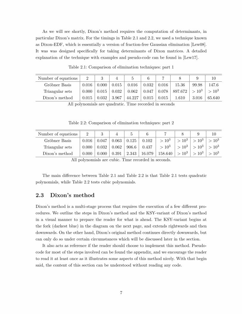
As we will see shortly, Dixon’s method requires the computation of determinants, inparticular Dixon’s matrix. For the timings in Table 2.1 and 2.2, we used a technique knownas Dixon-EDF, which is essentially a version of fraction-free Gaussian elimination [Lew08].It was was designed specifically for taking determinants of Dixon matrices. A detailedexplanation of the technique with examples and pseudo-code can be found in [Lew17].

Table 2.1: Comparison of elimination techniques: part 1

Number of equations 2 3 4 5 6 7 8 9 10Gröbner Basis 0.016 0.000 0.015 0.016 0.032 0.016 15.36 99.98 147.6Triangular sets 0.000 0.015 0.032 0.062 0.047 0.078 897.672 > 103 > 103

Dixon’s method 0.015 0.032 3.967 44.227 0.015 0.015 1.610 3.016 65.640All polynomials are quadratic. Time recorded in seconds

Table 2.2: Comparison of elimination techniques: part 2

Number of equations 2 3 4 5 6 7 8 9 10Gröbner Basis 0.016 0.047 0.063 0.125 0.102 > 103 > 103 > 103 > 103

Triangular sets 0.000 0.032 0.062 906.6 0.437 > 103 > 103 > 103 > 103

Dixon’s method 0.000 0.000 0.391 2.343 16.079 158.640 > 103 > 103 > 103

All polynomials are cubic. Time recorded in seconds.

The main difference between Table 2.1 and Table 2.2 is that Table 2.1 tests quadraticpolynomials, while Table 2.2 tests cubic polynomials.

2.3 Dixon’s method

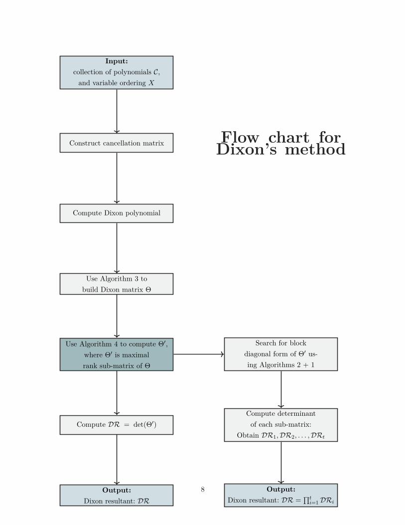
Dixon’s method is a multi-stage process that requires the execution of a few different pro-cedures. We outline the steps in Dixon’s method and the KSY-variant of Dixon’s methodin a visual manner to prepare the reader for what is ahead. The KSY-variant begins atthe fork (darkest blue) in the diagram on the next page, and extends rightwards and thendownwards. On the other hand, Dixon’s original method continues directly downwards, butcan only do so under certain circumstances which will be discussed later in the section.

It also acts as reference if the reader should choose to implement this method. Pseudo-code for most of the steps involved can be found the appendix, and we encourage the readerto read it at least once as it illustrates some aspects of this method nicely. With that beginsaid, the content of this section can be understood without reading any code.

7

Input:collection of polynomials C,and variable ordering X

Construct cancellation matrix Flow chart forDixon’s method

Compute Dixon polynomial

Use Algorithm 3 tobuild Dixon matrix Θ

Use Algorithm 4 to compute Θ′,where Θ′ is maximalrank sub-matrix of Θ

Search for blockdiagonal form of Θ′ us-ing Algorithms 2 + 1

Compute determinantof each sub-matrix:

Obtain DR1,DR2, . . . ,DRt

Output:Dixon resultant: DR =

∏ti=1DRi

Compute DR = det(Θ′)

Output:Dixon resultant: DR

8

Arriving at the Dixon resultant involves three major steps. Throughout our research,we used the Kapur-Saxena-Yang variant of the Dixon resultant [Lew96]. The first stepis to construct what is known as the cancellation matrix [CK02]. The determinant of thecancellation matrix is the Dixon polynomial. The Dixon polynomial acts as an intermediarystage between the cancellation matrix and the Dixon matrix. To produce the Dixon matrixfrom the Dixon polynomial, one needs to rewrite the Dixon polynomial as a special vector-matrix-vector product. The matrix produced in this product is called the Dixon matrix.

Beginning with a system of n+1 equations F = {f0, . . . , fn}, we must select n variablesX = [x1, . . . , xn] to eliminate. We call the list variables in the list X the set of originalvariables. The order of these variables can affect the size and degree of of the Dixon polyno-mial. For this reason we denote the Dixon polynomial of a given system F as ∆(F , X), toemphasize that the Dixon polynomial depends on both F and X. Literature on selecting theoptimal order to eliminate the variables does exist but will not be the focus of this thesis.See [CK02] for more information. Once a variable ordering is chosen, we can compute theDixon polynomial using the following formula:

Definition 2.3.1. [CK02] Let π(xα) = x̄α11 · · · x̄

αii x

α+1i+1 · · ·x

αdd , for i ∈ {0, . . . , d}, and x̄i’s

are new variables; π0(xα) = xα. We extend π to polynomials as: πi(f(x1, x2, . . . , xd)) =f(x̄1, . . . , x̄i, xi+1, . . . , xd). We define the Dixon polynomial as:

∆(F , X) =n∏i=1

1xi − x̄i

∣∣∣∣∣∣∣∣∣∣∣∣∣

π0(f0) π0(f1) π0(f2) . . . π0(fn)

π1(f0) π1(f1) π1(f2) . . . π1(fn)...

......

...

πn(f0) πn(f1) πn(f2) . . . πn(fn)

∣∣∣∣∣∣∣∣∣∣∣∣∣(2.3)

The matrix in definition 2.3.1 is the cancellation matrix of F with respect to a particularvariable elimination order X. Hence we denote this matrix with CF ,X . Since for all 1 ≤i ≤ n, (xi − x̄i) is a zero of CF ,X ,

∏ni=1(xi − x̄i) divides CF ,X [Kap97]. Hence ∆(F , X)

is a polynomial, which we call the Dixon polynomial of F with respect to a particularelimination variable ordering of X. The Dixon polynomial can also tell us the dimension ofDixon’s matrix, which will be produced in the next stage.

Definition 2.3.2. [Kap97] Let V be a row vector of all monomials in X which appearin ∆(F , X), when ∆(F , X) is viewed as a polynomial in X. Similarly, Let W be a columnvector of all monomials in X̄ which appear in ∆(F , X), when ∆(F , X) is viewed as apolynomial in X̄. The Dixon matrix, Θ, of F is defined to be the matrix for which∆(F , X) = VΘW. The entries of the Dixon matrix for F are polynomials in the coefficientsof F . Dixon’s matrix is an

∏ni=1(ei+1)×

∏ni=1(di+1) matrix, where ei = deg(∆(F , X), xi),

and di = deg(∆(F , X), x̄i).

9

The Dixon resultant is the determinant of Dixon’s matrix. Technically speaking, theDixon resultant is not a resultant as we defined it in Definition 1.2.1. It is a non-zero multipleof the resultant of a given system.

Let C be a collection of polynomials in the variables X, with parameters c. Let I bethe ideal generated by C in the ring k[X, c], and let J = I ∩ k[c]. Then J is the eliminationideal of I over c, and all polynomials h ∈ J are known as the projection operators of Cwith respect to X [Kap97]. The Dixon resultant is a member of J , or a projection operatorof C. It can be shown that the resultant of C also belongs to J , and divides all projectionoperators. Hence every Dixon resultant contains as one of its factors the resultant of C withrespect to a particular set of variables X [Kap97]. All factors of a Dixon resultant thatare not the resultant are called extraneous factors [Kap97]. A Dixon resultant that doesnot contain any extraneous factors is called exact [Kap97]. Identifying extraneous factorsin Dixon resultants is not trivial, especially when the Dixon resultants are large. Furtherinformation about extraneous factors can be found in [KS97].

As was discussed by Dixon himself, his method is only defined if the system of polyno-mials equations is generic and n-degree [Dix08], [Dix09].

Definition 2.3.3. [Kap97] A collection of polynomials C = {f1, . . . , fn+1} is called genericn-degree if there exists non-negative integers d1, . . . , dn such that,

fj =d1∑i1=0· · ·

dn∑in=0

aj,i1,...,inxi11 · · ·x

inn for 1 ≤ j ≤ n+ 1

where each coefficient aj,i1,...,inxi11 · · ·xinn is a distinct indeterminate. The n-tuple (d1, . . . , dn)

is known as their n-degree.

This limits us to a small class of systems. One reason is because if this condition doesnot hold, then using the formula in Definition 2.3.2 it is not hard to show that Dixon’smatrix will not be square. Dixon’s original method only allows us to take determinants ofsquare matrices, so if Θ is not square we are stuck. Additionally, Θ could be square butrank deficient, which means its determinant is identical to zero [Dym13]. This gives us noinformation about the system in question.

The Kapur-Saxena-Yang variant [KS95] of Dixon’s method gives us the necessary tools tosidestep both of these problems. Once the Dixon matrix Θ of C is constructed, we search fora sub-matrix of maximal rank Θ′ within Θ. Not only is Θ′ guaranteed to be square [Lay06],but given that certain conditions are satisfied, det(Θ′) is a non-zero projection operator ofC. This is stated nicely in the theorem below. An algorithm to search for a sub-matrix ofmaximal rank is provided in the appendix (Algorithm 4).

Theorem 2.3.4 (Kapur-Saxena-Yang). [Lew96] Let DR be the determinant of any maxi-mal rank sub-matrix of Θ. Then, if a certain condition holds, DR = 0 is necessary for theexistence of a common zero.

10

In short, this theorem is saying that if a system F generates a rank deficient Dixon matrixΘ, including the possibility of Θ begin non-square, then the determinant of any maximalrank sub-matrix of Θ will be a projection operator of F . Theorem 2.3.4 provides us withthe means to compute the Dixon resultant of arbitrary systems of polynomial equations.

So once we produce a Dixon resultant, what can we do with it? We mentioned earlyin the introduction that under certain circumstances the resultant of a polynomial systemgives us information about what the solution to the entire system looks like. We formalizethat notion with a central theorem.

Theorem 2.3.5 (Fundamental Theorem of Resultants). [GCL92, chapter 9] Let k̄ be analgebraically closed field, and let

f =m∑i=0

ai(x2, . . . , xr)xi1, g =n∑i=0

bi(x2, . . . , xr)xi1 (2.4)

be elements of k̄[x1, . . . , xr] of positive degrees in x1. Then if (α1, . . . , αr) is a common zeroof f and g, their resultant with respect to x1 satisfies

Res(f, g, x1)(α2, . . . , αr) = 0. (2.5)

Conversely, if the above resultant vanishes at (α2, . . . , αr), then at least one of the fol-lowing holds:

1. am(α2, . . . , αr) = · · · = a0(α2, . . . , αr)

2. bn(α2, . . . , αr) = · · · = b0(α2, . . . , αr)

3. am(α2, . . . , αr) = bn(α2, . . . , αr) = 0

4. ∃α1 ∈ x̄ such that (α1, α2, . . . , αr) is a common zero of f and g.

This theorem provides us with a way to use resultants to construct partial solutions tosystems of polynomial equations, which under certain circumstances lead to the full solu-tion. If the first three conditions of Theorem 2.3.5 do not hold, then Condition 4 guaranteesus that we are able to extend a partial solution one more coordinate position. Hence pro-ducing a resultant can be thought of as simplifying the problem of finding the solution tomany polynomial equations at once, to finding the solution of a single polynomial in fewervariables.

Before we end this chapter, we want to do a small example with Dixon’s method so thatwe become comfortable with the sequence of procedures. The flow chart was presented onpage 8 if it is needed for reference.

11

2.4 The area of a triangle

c = 6

a = 5b = 5

A =?

γ α

β

Figure 2.1: Heron’s problem [not drawn to scale]

Our goal is to determine the area of a triangle without computing any of its angles. We willassume that the side lengths we are given are in fact valid side lengths of a triangle. Onecan easily check this by verifying that the follow three inequalities hold:

a+ b > c, a+ c > b, b+ c > a

It is important to check this since this problem does not make sense if there does not exista triangle with the given side lengths to begin with. These inequalities tell us for whichvalues we are allowed to specialize Dixon’s resultant; essentially only values which producea valid triangle.

We begin by setting up a system of polynomial equations which correspond to thegeometric nature of this problem. We will not detail the process of constructing a systemof polynomial equations from a geometric problem, however [CLO15, Chapter 6] has anintroduction to geometric theorem proving which provides a concrete example.

Example 2.4.1. Let F = {x2 + y2− c2, (x− a)2 + y2− b2, 2A− ay}. Let X = [x, y] be thevariables which we wish to eliminate, our new variables X̄ = [x̄1, x̄2] and the parametersc = {A, a, b, c}. Note that both X and X̄ are ordered lists, and correspond to the orderwe are eliminating the variables. Simply put, the polynomials in F provide an algebraicdescription of the problem we are trying to solve.Using the formula in 2.3.1 we get:

∆ = ∆(F , X) =2∏i=1

1xi − x̄i

∣∣∣∣∣∣∣∣∣∣−c2 + x2 + y2 (x− a)2 + y2 − b2 −ay + 2A

−y − x̄1 −y − α1 a

−x− x̄2 −x+ 2a− x̄2 0

∣∣∣∣∣∣∣∣∣∣(2.6)

12

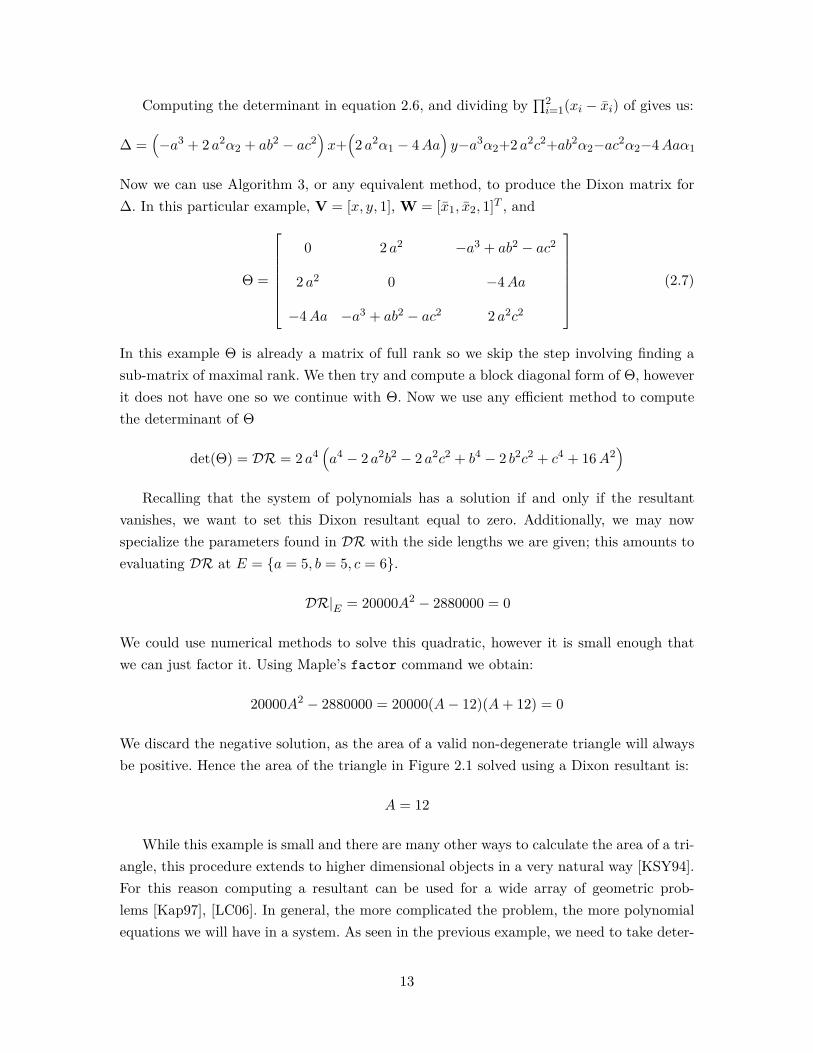
Computing the determinant in equation 2.6, and dividing by∏2i=1(xi − x̄i) of gives us:

∆ =(−a3 + 2 a2α2 + ab2 − ac2

)x+(2 a2α1 − 4Aa

)y−a3α2+2 a2c2+ab2α2−ac2α2−4Aaα1

Now we can use Algorithm 3, or any equivalent method, to produce the Dixon matrix for∆. In this particular example, V = [x, y, 1], W = [x̄1, x̄2, 1]T , and

Θ =

0 2 a2 −a3 + ab2 − ac2

2 a2 0 −4Aa

−4Aa −a3 + ab2 − ac2 2 a2c2

(2.7)

In this example Θ is already a matrix of full rank so we skip the step involving finding asub-matrix of maximal rank. We then try and compute a block diagonal form of Θ, howeverit does not have one so we continue with Θ. Now we use any efficient method to computethe determinant of Θ

det(Θ) = DR = 2 a4(a4 − 2 a2b2 − 2 a2c2 + b4 − 2 b2c2 + c4 + 16A2

)Recalling that the system of polynomials has a solution if and only if the resultant

vanishes, we want to set this Dixon resultant equal to zero. Additionally, we may nowspecialize the parameters found in DR with the side lengths we are given; this amounts toevaluating DR at E = {a = 5, b = 5, c = 6}.

DR|E = 20000A2 − 2880000 = 0

We could use numerical methods to solve this quadratic, however it is small enough thatwe can just factor it. Using Maple’s factor command we obtain:

20000A2 − 2880000 = 20000(A− 12)(A+ 12) = 0

We discard the negative solution, as the area of a valid non-degenerate triangle will alwaysbe positive. Hence the area of the triangle in Figure 2.1 solved using a Dixon resultant is:

A = 12

While this example is small and there are many other ways to calculate the area of a tri-angle, this procedure extends to higher dimensional objects in a very natural way [KSY94].For this reason computing a resultant can be used for a wide array of geometric prob-lems [Kap97], [LC06]. In general, the more complicated the problem, the more polynomialequations we will have in a system. As seen in the previous example, we need to take deter-

13

minants of matrices in order to obtain Dixon’s resultant. Furthermore, the matrices we areworking are over a polynomial ring. We need efficient methods to compute the determinantof symbolic matrices if we hope to produce Dixon resultants for large systems. This leadsus into Chapter 3, as we explore determinant computation.

14

Chapter 3

Determinants

3.1 An overview of methods

Let us start with Gaussian elimination which is taught in a first linear algebra course as amethod for calculating the determinant of a matrix. Gaussian elimination needs divisions,and thus requires a field. For an n × n matrix it does O(n3) field operations. When ap-plied to a symbolic matrix, Gaussian elimination produces rational functions which growin size/degree with each elimination step. These expressions require the computation ofpolynomial gcds to simplify. These operations can be expensive even for small matrices.

In this chapter, we consider two other methods that compute the determinant of amatrix using only the ring operations addition, subtraction, and multiplication. The cost ofthe methods are shown below for convenient reference.

Algorithm Number of ring/field operations

Gaussian Elimination O(n3)

Berkowitz O(n4)

Minor Expansion O(n2n)

The number of arithmetic operations in the table above do not account for the costof individual arithmetic operations, which may vary greatly. We will see in the followingsections that on symbolic matrices, the method of Minor expansion by Gentlemen & Johnsonis often the best choice despite the exponential number of operations it requires.

3.2 Minor expansion by Gentleman & Johnson

In this section we discuss the method of Minor expansion for computing determinants, whichalso goes by the names cofactor expansion or Laplace expansion. In 1973 paper [GJ73], tworesearchers Gentleman and Johnson noticed something peculiar about minor expansion.They noticed that for matrices of order 4 and larger, minor expansion computes certainexpressions multiple times. We use a short example with a matrix over the integers to

15

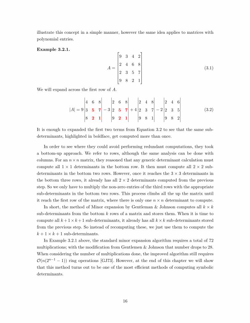
illustrate this concept in a simple manner, however the same idea applies to matrices withpolynomial entries.

Example 3.2.1.

A =

9 3 4 2

2 4 6 8

2 3 5 7

9 8 2 1

(3.1)

We will expand across the first row of A.

|A| = 9

∣∣∣∣∣∣∣∣∣∣4 6 8

3 5 7

8 2 1

∣∣∣∣∣∣∣∣∣∣− 3

∣∣∣∣∣∣∣∣∣∣2 6 8

2 5 7

9 2 1

∣∣∣∣∣∣∣∣∣∣+ 4

∣∣∣∣∣∣∣∣∣∣2 4 8

2 3 7

9 8 1

∣∣∣∣∣∣∣∣∣∣− 2

∣∣∣∣∣∣∣∣∣∣2 4 6

2 3 5

9 8 2

∣∣∣∣∣∣∣∣∣∣(3.2)

It is enough to expanded the first two terms from Equation 3.2 to see that the same sub-determinants, highlighted in boldface, get computed more than once.

In order to see where they could avoid performing redundant computations, they tooka bottom-up approach. We refer to rows, although the same analysis can be done withcolumns. For an n×n matrix, they reasoned that any generic determinant calculation mustcompute all 1 × 1 determinants in the bottom row. It then must compute all 2 × 2 sub-determinants in the bottom two rows. However, once it reaches the 3 × 3 determinants inthe bottom three rows, it already has all 2 × 2 determinants computed from the previousstep. So we only have to multiply the non-zero entries of the third rows with the appropriatesub-determinants in the bottom two rows. This process climbs all the up the matrix untilit reach the first row of the matrix, where there is only one n× n determinant to compute.

In short, the method of Minor expansion by Gentleman & Johnson computes all k × ksub-determinants from the bottom k rows of a matrix and stores them. When it is time tocompute all k+ 1×k+ 1 sub-determinants, it already has all k×k sub-determinants storedfrom the previous step. So instead of recomputing these, we just use them to compute thek + 1× k + 1 sub-determinants.

In Example 3.2.1 above, the standard minor expansion algorithm requires a total of 72multiplications; with the modification from Gentlemen & Johnson that number drops to 28.When considering the number of multiplications done, the improved algorithm still requiresO(n(2n−1 − 1)) ring operations [GJ73]. However, at the end of this chapter we will showthat this method turns out to be one of the most efficient methods of computing symbolicdeterminants.

16

3.3 Characteristic polynomials by Berkowitz

The Samuelson-Berkowitz algorithm is an efficient method of computing the characteristicpolynomial of an n× n matrix. It is particularly useful in our case because the Samuelson-Berkowitz algorithm well behaved when the entries of the matrix belong to any unitalcommutative ring without zero divisors. Given an n×n matrix, it recursively partitions thematrix into principal sub-matrices until it reaches the 1 × 1 sub-matrix in the upper lefthand corner. It then assembles the coefficients of the characteristic polynomial by takingsuccessively larger vector-matrix products. The Samuelson-Berkowitz algorithm stands asone of the most efficient ways to compute the characteristic polynomial of an n× n matrixover a ring. As was mentioned early in this chapter, the algorithm requires O(n4) ringoperations.

So how does computing the characteristic polynomial relate to determinants? To answerthis question, we need to look at the definition of the characteristic polynomial.

Definition 3.3.1. Consider an n × n matrix A ∈ Fn×n. The characteristic polynomial ofA, denoted by pA(x), is the polynomial defined by

n∑i=0

aixi = pA(x) = det(xI −A).

where I denotes the n× n identity matrix.

The characteristic polynomial pA(x) is a polynomial in x, with coefficients from thedomain which the matrix is defined over. In addition, definition 3.3.1 will produce a monicpolynomial. The eigenvalues of A are the roots of pA(x), and so we may write:

pA(x) = (x− λ1)(x− λ2) · · · (x− λn) =n∏i=1

(x− λi). (3.3)

We can easily show that the constant term in the expansion of the characteristic poly-nomial of A is in fact the determinant of A. Consider what would happen it we set x = 0in Equation 3.3.

a0 =n∏i=1

λi = pA(0) = det(0I −A) = det(−A) = −det(A).

It follows that the constant term of pA is, up to a unit, the determinant of the A. Tosummarize, the Samuelson-Berkowitz algorithm for computing the characteristic polynomialof a matrix acts as a vehicle for producing determinants.

17

3.4 A comparison of methods

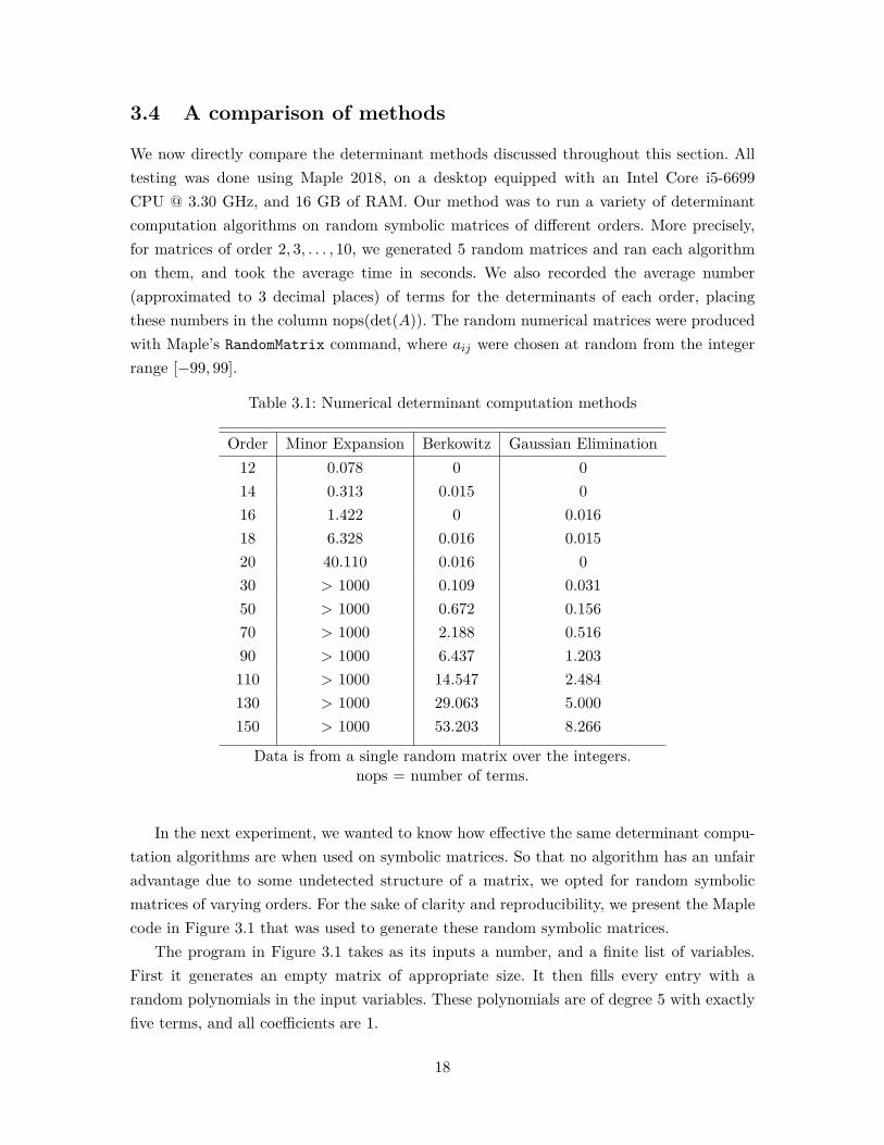
We now directly compare the determinant methods discussed throughout this section. Alltesting was done using Maple 2018, on a desktop equipped with an Intel Core i5-6699CPU @ 3.30 GHz, and 16 GB of RAM. Our method was to run a variety of determinantcomputation algorithms on random symbolic matrices of different orders. More precisely,for matrices of order 2, 3, . . . , 10, we generated 5 random matrices and ran each algorithmon them, and took the average time in seconds. We also recorded the average number(approximated to 3 decimal places) of terms for the determinants of each order, placingthese numbers in the column nops(det(A)). The random numerical matrices were producedwith Maple’s RandomMatrix command, where aij were chosen at random from the integerrange [−99, 99].

Table 3.1: Numerical determinant computation methods

Order Minor Expansion Berkowitz Gaussian Elimination12 0.078 0 014 0.313 0.015 016 1.422 0 0.01618 6.328 0.016 0.01520 40.110 0.016 030 > 1000 0.109 0.03150 > 1000 0.672 0.15670 > 1000 2.188 0.51690 > 1000 6.437 1.203110 > 1000 14.547 2.484130 > 1000 29.063 5.000150 > 1000 53.203 8.266

Data is from a single random matrix over the integers.nops = number of terms.

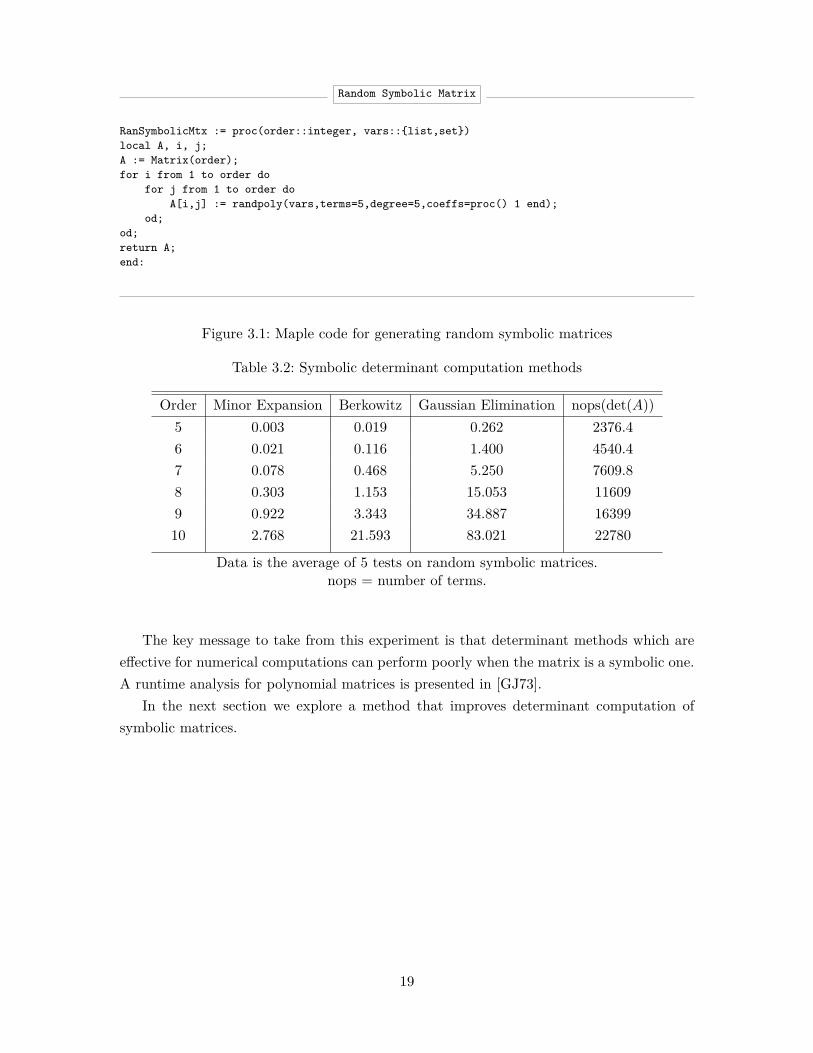
In the next experiment, we wanted to know how effective the same determinant compu-tation algorithms are when used on symbolic matrices. So that no algorithm has an unfairadvantage due to some undetected structure of a matrix, we opted for random symbolicmatrices of varying orders. For the sake of clarity and reproducibility, we present the Maplecode in Figure 3.1 that was used to generate these random symbolic matrices.

The program in Figure 3.1 takes as its inputs a number, and a finite list of variables.First it generates an empty matrix of appropriate size. It then fills every entry with arandom polynomials in the input variables. These polynomials are of degree 5 with exactlyfive terms, and all coefficients are 1.

18

Random Symbolic Matrix

RanSymbolicMtx := proc(order::integer, vars::{list,set})local A, i, j;A := Matrix(order);for i from 1 to order do

for j from 1 to order doA[i,j] := randpoly(vars,terms=5,degree=5,coeffs=proc() 1 end);

od;od;return A;end:

Figure 3.1: Maple code for generating random symbolic matrices

Table 3.2: Symbolic determinant computation methods

Order Minor Expansion Berkowitz Gaussian Elimination nops(det(A))5 0.003 0.019 0.262 2376.46 0.021 0.116 1.400 4540.47 0.078 0.468 5.250 7609.88 0.303 1.153 15.053 116099 0.922 3.343 34.887 1639910 2.768 21.593 83.021 22780

Data is the average of 5 tests on random symbolic matrices.nops = number of terms.

The key message to take from this experiment is that determinant methods which areeffective for numerical computations can perform poorly when the matrix is a symbolic one.A runtime analysis for polynomial matrices is presented in [GJ73].

In the next section we explore a method that improves determinant computation ofsymbolic matrices.

19

Chapter 4

Algorithms for revealing blockstructure

This chapter contains information pertaining to the algorithm we developed, and constitutesour main contribution.

4.1 Divide and Conquer

Divide and Conquer is an algorithm design paradigm that revolves around breaking downa given problem into at least two smaller sub-problems. In problems well suited to thisparadigm, the smaller sub-problems are easier to solve. We will not have a comprehensivediscussion about which algorithms are well suited for Divide and Conquer, however thereis one application in which using the paradigm of Divide and Conquer pays dividends.

We will define block matrices in general, however throughout this section we will onlymake reference to either block diagonal matrices or block diagonal triangular matrices. Thedeterminant properties we are interested in apply to both upper and lower block triangularmatrices.

Definition 4.1.1. [Dym13, Chapter 1] A matrix A ∈ Fn×n with block decomposition

A =

A11 · · · A1k...

...

Ak1 · · · Akk

where Aij ∈ Fpi×qj for i, j = 1, . . . , k and p1 + · · ·+ pk = q1 + · · ·+ qk = n is said to be:

• upper block triangular if pi = qi for i = 1, . . . , k and Aij = O for i > j.

• lower block triangular if pi = qi for i = 1, . . . , k and Aij = O for i < j.

• block triangular if it is either upper block triangular or lower block triangular.

20

• block diagonal if pi = qi for i = 1, . . . , k and Aij = O for i 6= j.

Note that the blocks Aii in a block triangular decomposition need not be triangular.

Certain Dixon matrices Θ′ have a block triangular form. By block triangular form, wemean that there exists some permutation of the rows and columns of the matrix such that thematrix now satisfies one of the statements in Definition 4.1.1. We consider block diagonalmatrices a special subset of block triangular matrices. Knowing if a matrix has a blocktriangular form is important because we know that the determinant of such a matrix is theproduct of the determinants of the square sub-matrices along its main diagonal [Dym13,Chapter 5]. Using the notation for Dixon matrices, rather then computing det(Θ′), weemploy a Divide and Conquer strategy, and compute the determinant of each sub-matrixalong the main diagonal. Even better, the computation of the determinant of each sub-matrix can be done in parallel, since the computations are now independent of one another.This can provide significant savings in computational resources as the matrices becomelarge. We do not have necessary and sufficient conditions as to which systems of polynomialequations produce Dixon matrices that have a block triangular form.

Before we give an explanation of the algorithm, we would like to justify the claim thatcomputing a block diagonal form using our algorithm does actually result in faster deter-minant computation. Figure 4.1 shows the expected speed-up for computing determinantswhen computing the determinants of the blocks as opposed to the entire matrix at once.We have plotted in number of blocks on the x-axis, the order of the matrix on the y-axis,and the speed-up achieved on the vertical axis.

In the following two sections we will outline our method. The algorithms unfolds in twophases, with the possibility of running the second phase without the first. For this reasonwe introduction the second phase of the algorithm before the first. This is also consistentwith how we actually developed the sub-routines during the course of our research. Phase1 is carried out by Algorithm 2, and we will refer to this algorithm as Clarify. Phase 2 iscarried out by Algorithm 1, and we refer to this algorithm as Link.

4.2 Phase 2: Link

The structure of a graph derived from a matrix can tell us many things about the ma-trix in question. With this in mind, we took inspiration for phase 2 of our new algorithmfrom [PF90]. In [PF90], they show a technique for computing the block diagonal form of arectangular matrix. Their method first creates a bipartite graph. Then it seeks to constructa maximal matching. Since our ultimate goal is to take the determinant of all the matriceswe work with, we only needed an algorithm for square matrices.

We create a bipartite graph that is based on the locations of the non-zero entries ineach row and column. To begin, let A be a k × k matrix of full rank where aij represents

21

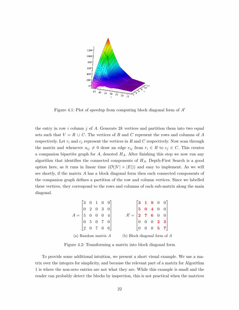
Figure 4.1: Plot of speedup from computing block diagonal form of A′

the entry in row i column j of A. Generate 2k vertices and partition them into two equalsets such that V = R ∪ C. The vertices of R and C represent the rows and columns of Arespectively. Let ri and cj represent the vertices in R and C respectively. Now scan throughthe matrix and whenever aij 6= 0 draw an edge eij from ri ∈ R to cj ∈ C. This createsa companion bipartite graph for A, denoted HA. After finishing this step we now run anyalgorithm that identifies the connected components of HA. Depth-First Search is a goodoption here, as it runs in linear time (O(|V | + |E|)) and easy to implement. As we willsee shortly, if the matrix A has a block diagonal form then each connected components ofthe companion graph defines a partition of the row and column vertices. Since we labelledthese vertices, they correspond to the rows and columns of each sub-matrix along the maindiagonal.

A =

3 0 1 0 90 2 0 3 05 0 0 0 40 5 0 7 02 0 7 0 6

(a) Random matrix A

A′ =

3 1 9 0 05 0 4 0 02 7 6 0 00 0 0 2 30 0 0 5 7

(b) Block diagonal form of A

Figure 4.2: Transforming a matrix into block diagonal form

To provide some additional intuition, we present a short visual example. We use a ma-trix over the integers for simplicity, and because the relevant part of a matrix for Algorithm1 is where the non-zero entries are not what they are. While this example is small and thereader can probably detect the blocks by inspection, this is not practical when the matrices

22

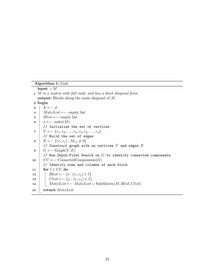
Algorithm 1: Linkinput : M

1 M is a matrix with full rank, and has a block diagonal formoutput: Blocks along the main diagonal of M

2 begin3 E ←− ∅4 MatxList←− empty list5 Blist←− empty list6 n←− order(M)

// Initialize the set of vertices7 V ←− {r1, r2, . . . , rn, c1, c2, . . . , cn}

// Build the set of edges8 E ←− {(ri, cj) : Mi,j 6= 0}

// Construct graph with on vertices V and edges E9 G←− Graph(V,E)

// Run Depth-First Search on G to identify connected components10 CC ←− ConnectedComponents(G)

// Identify rows and columns of each block11 for ` ∈ CC do12 Rlist←− {i : (ri, cj) ∈ `}13 Clist←− {j : (ri, cj) ∈ `}14 MatxList←−MatxList ∪ SubMatrix(M,Rlist, Clist)15 return MatxList

23

get large.

Example 4.2.1. Consider the following matrix:

A =

3 16 0 15 0

0 0 32 0 9

2 14 0 41 0

0 0 17 0 16

27 21 0 33 0

(4.1)

Our goal here is to determine if the rows and columns of A can be permuted in such away that it is either in block diagonal form, or upper block diagonal form. If this is in factpossible, we would also like to know which rows and column belong to each block. Link

begins by producing the bipartite graph in figure 4.3a.

(a) Bipartite construction of matrix A (b) Bipartite construction of matrix A′

Now we can run any algorithm that identifies the connected components of this graph.Depth-First Search is a good choice as it runs in O(|V | + |E|). If we let n be the orderof the matrix A, then |V | = 2n and |E| = hn2 for some h constant h ∈ Q. Since HA is abipartite graph, it can have at most n2 edges. The matrices we usually work with are sparse,so h could be as small as 1

20 . Hence O(|V |+ |E|) simplifies to O(2n+ hn2) = O(n+ hn2).Algorithm 1 runs Maple’s ConnectedComponents command which gives us:

L = [[c1, c2, c4, r1, r3, r5], [c3, c5, r2, r4]] .

24

This tells us that the first block is of order 3, defined by the rows 1, 3, 5 and columns 1, 2, 4.The second block is identified in the same manner. With this information we can nowpermute the rows and columns of A to reveal the block structure. The rows and columnsneed to be permuted in the order that we see the indices in L. So the row and columnpermutations are:rows:

rows:[1, 2, 3, 4, 5]→ [1, 3, 5, 2, 4] columns:[1, 2, 3, 4, 5]→ [1, 2, 4, 3, 5]

.This results in:

A′ =

3 16 15 0 0

2 14 41 0 0

27 21 33 0 0

0 0 0 32 9

0 0 0 17 16

(4.2)

If we run Link on A′, the companion graph HA′ is shown in figure 4.3b.

Now we can clearly see the two connected components of the graph. This is the intuitivereason why this algorithm works without having to permute rows and columns. This is alsothe reason why Link fails when the matrix has a block triangular but not strictly blockdiagonal. The entries that do not belong to the blocks on the diagonal create "bridges"from one block to another. This effectively puts an edge from one connected component toanother, and prevents any connected components algorithm from differentiating betweenmultiple blocks. Fortunately we have a solution in that case, and it is the main topic ofdiscussion in the next section.

4.3 Phase 1: Clarify

4.3.1 Upper block triangular matrices

Now suppose we are given a matrix that has a block triangular form, but not a strictlyblock diagonal form. The difference here begin that there exists some non-zero entries inblocks above the main diagonal. It can be shown that the determinant of these matricesis also the product of the determinant of the matrices along the main diagonal. In otherwords the determinant of such a matrix does not depend on the entries in blocks off themain diagonal. If we use Algorithm 1 as seen in the previous section, it will fail to reliably

25

identify any block structure. An example illustrates what must occur in order for us toretrieve the blocks in this case.

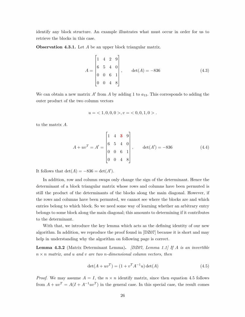
Observation 4.3.1. Let A be an upper block triangular matrix.

A =

1 4 2 9

6 5 4 0

0 0 6 1

0 0 4 8

, det(A) = −836 (4.3)

We can obtain a new matrix A′ from A by adding 1 to a13. This corresponds to adding theouter product of the two column vectors

u = < 1, 0, 0, 0 >, v = < 0, 0, 1, 0 > .

to the matrix A.

A+ uvT = A′ =

1 4 3 9

6 5 4 0

0 0 6 1

0 0 4 8

, det(A′) = −836 (4.4)

It follows that det(A) = −836 = det(A′).

In addition, row and column swaps only change the sign of the determinant. Hence thedeterminant of a block triangular matrix whose rows and columns have been permuted isstill the product of the determinants of the blocks along the main diagonal. However, ifthe rows and columns have been permuted, we cannot see where the blocks are and whichentries belong to which block. So we need some way of learning whether an arbitrary entrybelongs to some block along the main diagonal; this amounts to determining if it contributesto the determinant.

With that, we introduce the key lemma which acts as the defining identity of our newalgorithm. In addition, we reproduce the proof found in [DZ07] because it is short and mayhelp in understanding why the algorithm on following page is correct.

Lemma 4.3.2 (Matrix Determinant Lemma). [DZ07, Lemma 1.1] If A is an invertiblen× n matrix, and u and v are two n-dimensional column vectors, then

det(A+ uvT ) = (1 + vTA−1u) det(A) (4.5)

Proof. We may assume A = I, the n × n identify matrix, since then equation 4.5 followsfrom A + uvT = A(I + A−1uvT ) in the general case. In this special case, the result comes

26

from the equality I 0

vT 1

I + uvT u

0 1

I 0

−vT 1

=

I u

0 1 + vTu

(4.6)

The main idea is as follows: given a matrix A over the integers we look at the locationof zeros in A−1 in order to set equal to zero entries in A without altering the determinantof A. If A is a symbolic matrix, then we induce an evaluation homomorphism on A, anddo the same thing on an image of A. The next sub-section will explain this idea in greaterdetail.

4.3.2 Explanation and proof for Clarify algorithm

Algorithm 2: Clarifyinput : A,n

1 A is an n× n matrix with full rank, n is order of A, with aij ∈ Z[x1, . . . , xt]output: A matrix M with det(M) = det(A), or the input matrix A

2 begin3 M ←− A4 Pick a suitably large prime, e.g 262 < p < 263

5 Pick γ = (γ1, . . . , γt) at random from Ftp6 B ←− Evaluate M at (xj = γj : 1 ≤ j ≤ t) mod p7 if rank(B) < n then8 Go back to line 4 // γ is unlucky

9 V ←− B−1 mod p10 for i← 1 to n do11 for j ← 1 to n do12 if vij = 0 then13 mji ←− 0

14 return M

Our new algorithm is comprised of two separate sub-routines. Usually Clarify (Algo-rithm 2) is run first, followed by Link (Algorithm 1). As we have seen it is possible thatLink can identify block structure without the use of Clarify. If the matrix has a blocktriangular form but not a strictly block diagonal form, then using Clarify is required forLink to return the blocks.

By Lemma 4.5, we have seen that we can update the determinant of a matrix withouthaving to compute another determinant. Clarify exploits this by checking if the following

27

equality holds:det(A+ uvT ) = (1 + vTA−1u) det(A) ?= det(A). (4.7)

In our implementation of Clarify, the column vectors u and v are always unit vectorswith exactly one non-zero entry; this is implicit as we do not perform any vector-matrixmultiplications. Clarify is a modular algorithm, as we perform all computations over afinite field Fp. Hence the inverse of B is computed modulo some prime p. This allows usto compute block diagonal forms of large matrices without creating massive numbers inB. Lastly, Clarify is a probabilistic algorithm, as it could happen that m−1

ij 6= 0 butvij = m−1

ij (γ) = 0. With this in mind, we introduce the Schwartz-Zippel Lemma, which willbe used in the approaching proof.

Lemma 4.3.3 (Schwartz-Zippel Lemma). Let f ∈ k[x1, x2, . . . , xn] be a non-zero polyno-mial of total degree d ≥ 0 over a field k. Let S be a finite subset of k and let r1, r2, . . . , rn

be selected at random independently and uniformly from S. Then

Prob[f(r1, r2, . . . , rn) = 0] ≤ d

|S|.

In order to explain Algorithm Clarify in greater detail, we will provide a proof ofcorrectness. This proof will not only show why the algorithm is correct, but also why it isimplemented in the way it has been.

Theorem 4.3.4. Let A be an n × n matrix of rank n, where aij ∈ Fp[x1, . . . , xt]. LetC = adj(A) and let B ≥ max deg(cij). Let p be the prime chosen in Algorithm Clarify.Then the output matrix M of Algorithm Clarify satisfies det(M) 6= det(A) with probabilityat most n2B

p .

Proof. Let C = adj(A). To use the Schwartz-Zippel Lemma, we need a degree bound B ≥deg(cij). We can use

B = min(n∑i=1

nmaxj=1

deg(cij),n∑j=1

nmaxi=1

deg(cij)).

Then deg(detA) ≤ B and deg(cij) ≤ B. Recall that A−1 = Cdet(A) . In algorithm Clarify,

V = A(γ)−1 = C(γ)det(A)(γ) and det(A)(γ) 6= 0. If cij 6= 0 but vij(γ) = 0, we say algorithm

Clarify is unlucky. We wish to determine the probability that Clarify outputs a matrixM with det(M) 6= det(A). This can happen in one of two ways. First, if a cij 6= 0 but

28

vij = 0, or in other words cij 6= 0 but cij(γ) ≡ 0 mod p. Then we have the following bound:

Prob[cij 6= 0 ∧ cij(γ) ≡ 0 mod p for some ij] ≤∏

1≤i,j≤nProb[cij 6= 0 ∧ cij(γ) ≡ 0 mod p]

≤n2 · max

1≤i,j≤ndeg(cij)

p

≤ n2B

p

The other way we could get unlucky is if the prime p divides every coefficient of det(A).Since we are working modulo p, this would cause the determinant to vanish. In practice thishas never occurred because usually the system of polynomial equations has small coefficientsto begin with. This in turn means the coefficients of the Dixon resultant will be relativelysmall. Given that p is of suitable size, it would be very unlikely for a non-zero coefficient tobelong to the residue class [0]. Overall, the bigger p is, the less likely Algorithm Clarify

will return a bad matrix M .

To summarize, if A has a block triangular form, then Clarify will delete all entries thatlie above/below the block diagonal; it transforms the matrix into one which has a blockdiagonal form without knowing first what that block diagonal form is. After Clarify is runof a matrix that has a block triangular form, the resulting matrix has a block diagonal form.We are now in the case where Link will correctly return all blocks along the main diagonal.

We finish this chapter with a small demonstration of Clarify.

Example 4.3.5. Let

A = M =

36y2 + 69 76 + 84y

0 62y + 1

, p = 997.

Clarify produces the following objects:

S = {x = 771, y = 218}, B =

81 442

0 556

, V =

837 493

0 945

.Looking at V , v21 = 0 indicates that we can set b12 equal to zero, which implies we can alsoset m12 equal to zero. Since v21 was the only entry that was identical to zero, AlgorithmClarify terminates and outputs:

M =

36y2 + 69 0

0 62y + 1

, det(M) = det(A).

29

Chapter 5

Empirical Results

We tested 15 polynomial systems using the KSY-variant of Dixon’s method, all coming fromreal-world geometric and scientific problems. For each system, we present an assortment ofinformation.

In Table 5.1, we show the number of polynomial equations in the system (Eqns), thenumber of variables which are to be eliminated (Vars), and the number of indeterminates inc (Pars). We also mention the size of the associated Dixon matrix Θ before we searched fora sub-matrix of maximal rank. After finding a sub-matrix Θ′ of Θ which has maximal rank,we recorded the rank of Θ′. Then we attempted to compute the upper block triangular orblock diagonal form of Θ′. We define the Sparsity of a matrix as the number of entries of amatrix that are zero, divided by the total number of entries in the matrix Θ′. The columnsTime (M.E) and Time (EDF) show the time it took to compute the determinant of thesmallest block along the main diagonal of Θ′. Finally nops(DR) shows the number of termsin a Dixon resultant of the corresponding system.

Table 5.2, Block Structure shows the sizes of the blocks along the main diagonal ofeach Θ′. Next to this column, Number of Multiplications shows how many polynomialmultiplications the method of Minor Expansion by Gentleman & Johnson [GJ73] requiresfor computing each sub-matrix along the main diagonal of Θ′. These two lists are orderedfrom left to right, and are in a one-to-one correspondence. For example, the first row of Table5.2 says that the Minor Expansion algorithm by Gentleman & Johnson requires 229568 and7767 multiplications to compute the determinants of the order 17 and order 12 blocks alongthe main diagonal respectively. Most importantly, the number of multiplications for eachsystem is within the computable range. We hope this provides some insight as to whatDixon matrices look like in practice.

30

Table5.1:

System

sInform

ationforDixon

matric

es+

Minor

Expa

nsionversus

Dixon

-EDF

System

Eqn

sVars\P

ars

dim

ΘRan

kSp

arsity

Tim

e(M

.E)

Tim

e(E

DF)

nops

(DR)

bricard

65/

1241×

4429

0.80

416

6.20

069

.80

1111

775

cath

edra

l†6

5/2

46×

4134

0.74

80.89

60.02

67

hero

n2d†

32/

43×

33

0.37

50.00

00.02

77

hero

n3d†

65/

716×

1413

0.76

90.00

10.00

823

hero

n4d†

109/

1110

3×

7563

0.94

10.02

60.04

314

71he

ron5

d15

14/1

670

7×

514

399

0.98

9!

36.39

?im

age2

d†6

5/6

32×

2929

0.90

70.00

00.00

522

imag

e3d†

109/

1017

8×

152

130

0.97

50.00

90.03

614

56im

age4

d†10

9/10

136×

126

120

0.97

60.00

80.02

370

4im

ageF

lex†

109/

1013

6×

126

120

0.97

60.00

60.02

370

4robo

tarm

s4

3/4

32×

3216

0.53

1!

3.38

?sys22

43/

926×

2622

0.73

655

6.2

519.6

3990

252

tot

32/

340×

4033

0.56

7!

46.78

?va

naub

el†

98/

628×

2828

0.89

33.22

00.21

832

166

Minor

Expa

nsiontim

ings

done

with

Map

le’s

implem

entatio

nof

Gentle

man

&Jo

hnson

†=

Projectio

nop

erator

compu

tableusingMap

le’s

Groe

bner

[Bas

is]comman

din<

1000

second

s

!=Ran

outof

mem

oryattemptingcalculation

31

Table5.2:

Block

structureof

Dixon

matric

es+

Minor

Expa

nsionmultip

licationcoun

t

System

Block

Structure

Num

berof

Multiplications

bricard

[17,12

][229

568,77

67]

cath

edra

l†[16,18

][170

905,95

5315

]he

ron2

d†[4]

[10]

hero

n3d†

[6,7]

[41,73

]he

ron4

d†[14,14

,17,18

][648

,159

2,19

078,46

586]

heron5

d[49,50

,52,49

,48,48

,50,53

][123

5007

8,?,?,20

2065

71,249

0507

8,?,?,?]

imag

e2d†

[10,7,7,5]

[111

,99,39

,39]

imag

e3d†

[13,14

,14,15

,18,19

,18,19

][575

,579

,346

2,91

4,45

27,711

8,14

777,47

37]

imag

e4d†

[13,14

,14,15

,17,16

,16,15

][945

,719

,150

5,66

4,68

72,421

5,50

43,357

5]im

ageF

lex†

[13,14

,14,15

,17,16

,16,15

][945

,719

,150

5,64

4,68

72,421

5,50

43,357

5]robo

tarm

s[8,8]

[728

,544

]sys22

[11,11

][409

0,42

76]

tot

[17,16

][890

695,44

2778

]va

naub

el†

[7,7,7,7]

[93,10

3,68

,39]

The

blockstructureof

asystem

issensitive

tothevaria

bleelim

inationorde

r

†=

Projectio

nop

erator

compu

tableusingMap

le’s

Groe

bner

[Bas

is]comman

din<

1000

second

s

32

Chapter 6

Conclusion

We begin the concluding chapter with two open research questions. While solving these isnot going to change the basic procedure we have outline in the paper, it could potentiallyincrease the speed at which we produce Dixon resultants.

Open Question 6.0.1. Does there exists sufficient conditions on a polynomial system Ffor its Dixon matrix to have a block diagonal form?

It is possible that these matrices have even more structure then what we currently knowabout. If we knew more about the polynomials that generated these matrices, we might beable to develop even better tools for taking the determinants of the Dixon matrices theygive rise to.

Open Question 6.0.2. For which systems are iterative resultant computation methodsmore efficient that Dixon’s method?

Dixon’s method simultaneously eliminates n variables from a system of n+1 polynomialequations. Another technique is to systematically eliminate one variables from the systemsone at a time using simpler resultant formulations such as Sylvester’s resultant. For largesystems of polynomial equations Dixon’s method seems to be the better choice, howeverit has not been well documented which techniques perform better for which systems ingeneral.

Resultant matrices have much to be discovered about them, but our hope is that wehave illuminated a fruitful research path for others. The algorithms and procedures fromChapter 2 should be implemented by those who are interested in learning more, as wefound a hands-on learning approach to this kind of work more effective. The key idea fromChapter 3 was that despite the seemingly prohibitive cost of the method of Minor expansion,it was the most effective algorithm with respect to symbolic determinant computation.Gentleman & Johnson demonstrated this beautifully when they showed that their versionof Minor expansion was actually the most effective when computing symbolic determinants

33

compared to methods which are superior in numerical computation. Chapter 4 containedour main results of the research project. Techniques and algorithms like Clarify and Link

were crucial for computing many of the symbolic determinants that otherwise would not bepossible. The implementation of Clarify was designed to be fast yet simple, and we havesuccessfully used it to locate blocks within matrices of up to order 1000.

We hope it is clear that resultants can aid in solving polynomial systems. They can easilyoutperform competing methods, such as Buchburger’s algorithm, if careful implementationis made. Since resultants computed from resultant matrices rely heavily on the speed atwhich we can compute symbolic determinants, high performance algorithms for computingsymbolic determinants are also of great interest. For those interested in learning more aboutcomputer algebra, see [GCL92] for an nice introduction. For those who are interested in amore rigorous treatment of the Dixon matrix, and Dixon resultants in general, consult[CK02], [Chi01], and [CK04]. For those interested in learning more about resultants, goodplaces to start would be [CLO15] and [Has07]. For more examples and applications of Dixonresultants see [Kap97], [Lew08], [LC06], [PZAG08], and [Lew17].

34

Bibliography

[Buc76] B. Buchberger. A theoretical basis for the reduction of polynomials to canonicalforms. ACM SIGSAM Bull., 10(3):19–29, 1976.

[Cay57] A. Cayley. Note sur la méthode d’élimination de Bezout. J. Reine Angew. Math.,53:366–367, 1857.

[Chi01] Eng-Wee Chionh. Rectangular corner cutting and Dixon A-resultants. J. Sym-bolic Comput., 31(6):651–669, 2001.

[CK02] Arthur D. Chtcherba and Deepak Kapur. On the efficiency and optimality ofDixon-based resultant methods. In Proceedings of the 2002 International Sym-posium on Symbolic and Algebraic Computation, pages 29–36. ACM, New York,2002.

[CK04] Arthur D. Chtcherba and Deepak Kapur. Constructing Sylvester-type resultantmatrices using the Dixon formulation. J. Symbolic Comput., 38(1):777–814, 2004.

[CLO15] David A. Cox, John Little, and Donal O’Shea. Ideals, varieties, and algorithms.Undergraduate Texts in Mathematics. Springer, Cham, fourth edition, 2015. Anintroduction to computational algebraic geometry and commutative algebra.

[Dix08] A. L. Dixon. On a Form of the Eliminant of Two Quantics. Proc. London Math.Soc. (2), 6:468–478, 1908.

[Dix09] A. L. Dixon. The Eliminant of Three Quantics in two Independent Variables.Proc. London Math. Soc. (2), 7:49–69, 1909.

[Dym13] Harry Dym. Linear algebra in action, volume 78 of Graduate Studies in Mathe-matics. American Mathematical Society, Providence, RI, second edition, 2013.

[DZ07] Jiu Ding and Aihui Zhou. Eigenvalues of rank-one updated matrices with someapplications. Appl. Math. Lett., 20(12):1223–1226, 2007.

[GCL92] K. O. Geddes, S. R. Czapor, and G. Labahn. Algorithms for computer algebra.Kluwer Academic Publishers, Boston, MA, 1992.

[GJ73] W. M. Gentleman and S. C. Johnson. Analysis of algorithms, a case study:determinants of polynomials. In Fifth Annual ACM Symposium on Theory ofComputing (Austin, Tex., 1973), pages 135–141. 1973.

[GKZ94] I. M. Gelfand, M. M. Kapranov, and A. V. Zelevinsky. Discriminants, resul-tants, and multidimensional determinants. Mathematics: Theory & Applica-tions. Birkhäuser Boston, Inc., Boston, MA, 1994.

35

[Has07] Brendan Hassett. Introduction to algebraic geometry. Cambridge UniversityPress, Cambridge, 2007.

[Kap97] Deepak Kapur. Automated geometric reasoning: Dixon resultants, gröbner bases,and characteristic sets. In Dongming Wang, editor, Automated Deduction inGeometry, pages 1–36, Berlin, Heidelberg, 1997. Springer Berlin Heidelberg.

[KS95] Deepak Kapur and Tushar Saxena. Comparison of various multivariate resultantformulations. In ISSAC, volume 95, pages 187–194. Citeseer, 1995.

[KS97] Deepak Kapur and Tushar Saxena. Extraneous factors in the Dixon resultantformulation. In Proceedings of the 1997 International Symposium on Symbolicand Algebraic Computation (Kihei, HI), pages 141–148. ACM, New York, 1997.

[KSY94] Deepak Kapur, Tushar Saxena, and Lu Yang. Algebraic and geometric reason-ing using Dixon resultants. In Proceedings of the international symposium onSymbolic and algebraic computation, pages 99–107. ACM, 1994.

[Lay06] David C Lay. Linear algebra and its applications. Third edition, 2006.

[LC06] Robert H Lewis and Evangelos A Coutsias. Algorithmic search for flexibilityusing resultants of polynomial systems. In International Workshop on AutomatedDeduction in Geometry, pages 68–79. Springer, 2006.

[Lew96] Robert H Lewis. The Kapur-Saxena-Yang variant of the Dixon resultant. 1996.

[Lew08] Robert H. Lewis. Heuristics to accelerate the Dixon resultant. Math. Comput.Simulation, 77(4):400–407, 2008.

[Lew17] Robert H. Lewis. Dixon-EDF: the premier method for solution of parametricpolynomial systems. In Applications of computer algebra, volume 198 of SpringerProc. Math. Stat., pages 237–256. Springer, Cham, 2017.

[Mac03] F. S. MacAulay. Some Formulae in Elimination. Proc. Lond. Math. Soc., 35:3–27,1903.

[Pal13] B. Paláncz. Application of Dixon resultant to satellite trajectory control by poleplacement. J. Symbolic Comput., 50:79–99, 2013.

[PF90] Alex Pothen and Chin-Ju Fan. Computing the block triangular form of a sparsematrix. ACM Trans. Math. Software, 16(4):303–324, 1990.

[PZAG08] Béla Paláncz, Piroska Zaletnyik, Joseph L Awange, and Erik W Grafarend.Dixon resultant’s solution of systems of geodetic polynomial equations. Journalof Geodesy, 82(8):505–511, 2008.

36

Appendix A

Code

Algorithm 3: BuildDixoninput : P = ∆(F , X), X, X̄

1 P is a Dixon polynomial, X = {x1, . . . , xn} is the set of original variables,X̄ = {x̄1, . . . , x̄n} is the set of new variablesoutput: Dixon matrix

2 begin3 BL←− list of monomials of P in the variables X4 BR←− list of monomials of P in the variables X̄5 r ←− |BL|6 c←− |BR|7 D ←− r × c zero matrix8 i←− 19 for m1 ∈ BL do

10 c1 ←− coeff(P,m1)11 j ←− 112 for m2 ∈ BR do13 Di,j ←− coeff(c1,m2)14 j ←− j + 115 i←− i+ 116 return BL, D, BR

Algorithm 3 constructs the dixon matrix for a given Dixon polynomial by separating thevariables from the parameters. Hence this matrix will be over k[c].

Algorithm 4 finds a sub-matrix of maximal rank. The SubMatrix command takes as itsinputs a matrix A, and two sets of integers L1 and L2 that define the rows and columns ofthe sub-matrix being extracted.

37

Algorithm 4: Chopinput : A,N,m, n

1 A is a Dixon matrix, N = {xn, a, b, . . .} is a list of t variables in A to be evaluated,m is the number of rows, n is the number of columnsoutput: Dixon matrix minor of full rank

2 begin3 Pick a suitably large prime p > 263

4 Pick γ = (γ1, . . . , γt) at random from Fp5 Evaluate the entries of A at γ6 A1←− A in row echelon form7 L1←− PivotColumns(A1)8 A2←− A in column echelon form9 L2←− PivotColumns(A2)

10 M ←− Submatrix(A,L1, L2)11 return M

38