kinematic variables for dark matter at the lhc and beyond
TRANSCRIPT

HARVARDUNIVERSITY
Christopher Rogan
Kinematic variables for Dark Matter at the LHC and Beyond
University of Chicago HEP Seminar – March 9, 2014

Christopher Rogan - University of Chicago HEP - March 9, 2015
▪ Weakly interacting particles at the LHC▪ Why? How?
▪ Kinematic handles for studying them▪ MET▪ singularity variables
▪ Recursive Jigsaw Reconstruction▪ ex. di-leptons (i.e. super-razor variables)▪ ex. di-leptonic tops/stops (something sexier)
2
Talk Outline

Christopher Rogan - University of Chicago HEP - March 9, 2015
▪ Why are they interesting?▪ Dark Matter▪ It exists - but what is it? Would like to know if
we’re producing these particles at the LHC▪ Electroweak bosons▪ Decays of W and Z often produce neutrinos
▪ New symmetries▪ Discrete symmetries (ex. R-parity) make
lightest new ‘charged’ particles stable
3
Weakly interacting particles @ LHC

Christopher Rogan - University of Chicago HEP - March 9, 2015
▪ How do we study them?▪ Can infer their presence through missing transverse energy▪ Hermetic design of LHC experiments allows us to infer
‘what’s missing’
4
Weakly interacting particles @ LHC
ATLAS Calorimeters ~EmissT = �
cellsX
i
~ET
▪ full azimuthal coverage, up to |Ƞ| of ~5
▪ stopping power of ~12-20 interaction lengths
▪ ECAL+HCAL components with segmentation comparable to lateral shower sizes

Christopher Rogan - University of Chicago HEP - March 9, 2015 5
CERN-LHCC-2006-021
Missing transverse energy [GeV]
Minimum bias data
∫ L dt = 11.7 nb-1
Missing transverse energy [GeV]
Figures from SUSY10 conference talk:
Missing transverse energy is a powerful observable for inferring the presence of weakly interacting particlesBut, it only tells us about their transverse momenta – often we can better resolve quantities of interest by using additional information
Missing transverse energy

Christopher Rogan - University of Chicago HEP - March 9, 2015 6
Missing transverse energy
?
Missing transverse energy only tells us about the momentum of weakly interacting particles in an event…Christopher Rogan - University of Chicago HEP - March 9, 2015

Christopher Rogan - University of Chicago HEP - March 9, 2015 7
Missing transverse energy
…not about the identity or mass of weakly interacting particles
Christopher Rogan - University of Chicago HEP - March 9, 2015

Christopher Rogan - University of Chicago HEP - March 9, 2015 8
Missing transverse energy
…not about the identity or mass of weakly interacting particles
Christopher Rogan - University of Chicago HEP - March 9, 2015

Christopher Rogan - University of Chicago HEP - March 9, 2015 9
Missing transverse energy
We can learn more by using other information in an event to contextualize the missing transverse energy
Christopher Rogan - University of Chicago HEP - March 9, 2015
Christopher Rogan - University of Chicago HEP - March 9, 2015 10
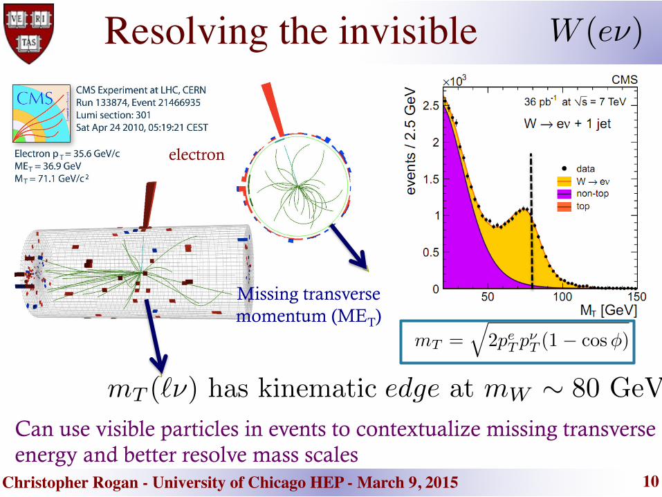
Resolving the invisible
electron
mT (`⌫) has kinematic edge at mW ⇠ 80 GeV
mT =
q2peT p
⌫T (1� cos�)
Missing transverse momentum (MET)
Can use visible particles in events to contextualize missing transverse energy and better resolve mass scales
W (e⌫)

Christopher Rogan - University of Chicago HEP - March 9, 2015 11
Missing transverse energy
We can learn more by using other information in an event to contextualize the missing transverse energy ⇒ multiple weakly interacting particles?
Christopher Rogan - University of Chicago HEP - March 9, 2015
Christopher Rogan - University of Chicago HEP - March 9, 2015
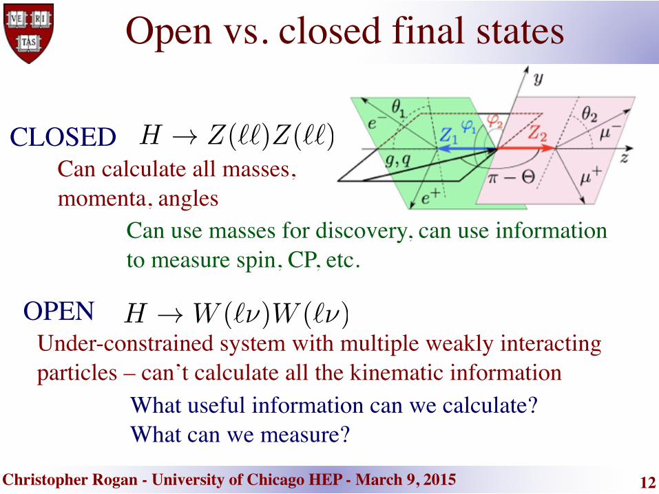
Open vs. closed final states
CLOSED
OPEN
Can calculate all masses, momenta, angles
Can use masses for discovery, can use information to measure spin, CP, etc.
Under-constrained system with multiple weakly interacting particles – can’t calculate all the kinematic information
What useful information can we calculate? What can we measure?
12

Christopher Rogan - University of Chicago HEP - March 9, 2015
Multiple weakly interacting particles?
S S
p
p
CM
visible
visible
invisible
invisible
Canonical open / topology
Can be single or multiple decays steps
Can be one or more particles
Can be one or more particles
TheorySUSY
Little HiggsUED
R-parityT-parity
KK-parity
▪ Dark Matter▪ Higgs quadratic
divergences▪ ….
13
Christopher Rogan - University of Chicago HEP - March 9, 2015
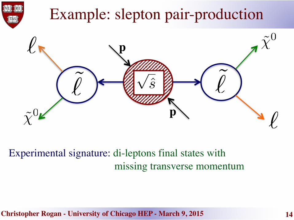
Example: slepton pair-production
p
p
CM
14
Experimental signature: di-leptons final states with missing transverse momentum
Christopher Rogan - University of Chicago HEP - March 9, 2015
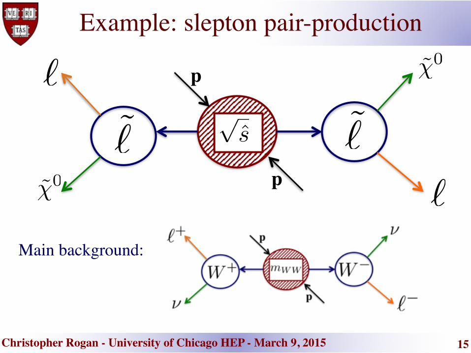
Example: slepton pair-production
p
p
CM
15
Main background:

Christopher Rogan - University of Chicago HEP - March 9, 2015
Example: slepton pair-production
p
p
CM
16
What quantities, if we could calculate them, could help us distinguish between signal and background events?

Christopher Rogan - University of Chicago HEP - March 9, 2015
Example: slepton pair-production
p
p
CM
17
What information are we missing?
We don’t observe the weakly interacting particles in the event. We can’t measure their momentum or masses.

Christopher Rogan - University of Chicago HEP - March 9, 2015
Example: slepton pair-production
p
p
CM
18
What do we know?
We can reconstruct the 4-vectors of the two leptons and the transverse momentum in the event

Christopher Rogan - University of Chicago HEP - March 9, 2015
Example: slepton pair-production
p
p
CM
19
Can we calculate anything useful?With a number of simplifying assumptions…
…we are still 4 d.o.f. short of reconstructing any masses of interest
~EmissT =
X~p �̃0
T m�̃0 = 0

Christopher Rogan - University of Chicago HEP - March 9, 2015
▪ State-of-the-art for LHC Run I was to use singularity variables as observables in searches
▪ Derive observables that bound a mass or mass-splitting of interest by▪ Assuming knowledge of event decay topology▪ Extremizing over under-constrained kinematic
degrees of freedom associated with weakly interacting particles
20
Singularity Variables
Christopher Rogan - University of Chicago HEP - March 9, 2015
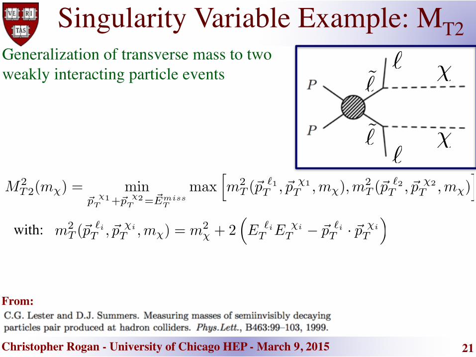
Singularity Variable Example: MT2
with:
From:
Generalization of transverse mass to two weakly interacting particle events
21
Christopher Rogan - University of Chicago HEP - March 9, 2015
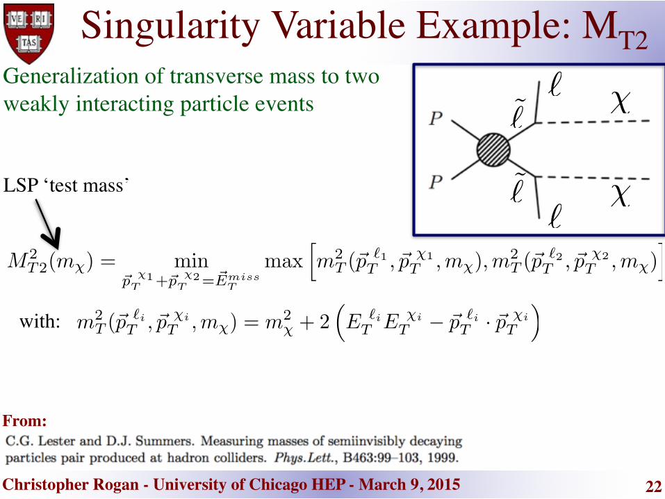
Singularity Variable Example: MT2
with:
LSP ‘test mass’
From:
Generalization of transverse mass to two weakly interacting particle events
22

Christopher Rogan - University of Chicago HEP - March 9, 2015
Singularity Variable Example: MT2
with:
LSP ‘test mass’
From:
Extremization of unknown degrees of freedom
Subject to constraints
Generalization of transverse mass to two weakly interacting particle events
23

Christopher Rogan - University of Chicago HEP - March 9, 2015
Singularity Variable Example: MT2
with:
LSP ‘test mass’
Constructed to have a kinematic endpoint (with the right test mass) at:From:
Extremization of unknown degrees of freedom
Subject to constraints
Generalization of transverse mass to two weakly interacting particle events
24
Mmax
T2
(m�) = m˜` Mmax
T2
(0) = M�
⌘m2
˜`�m2
�̃
m˜`

Christopher Rogan - University of Chicago HEP - March 9, 2015
MT2 in practice
ATLAS-CONF-2013-049
Backgrounds with leptonic W decays fall steeply once MT2 exceeds the W mass
Searches based on singularity variables have sensitivity to new physics signatures with mass splittings larger than the analogous SM ones
From:
25

Christopher Rogan - University of Chicago HEP - March 9, 2015
Recursive Jigsaw Reconstruction
▪ The strategy is to transform observable momenta iteratively reference-frame to reference-frame, traveling through each of the reference frames relevant to the topology
▪ At each step, extremize only the relevant d.o.f. related to that transformation
▪ Repeat procedure recursively, using only the momenta encountered in each reference frame
▪ Rather than obtaining one observable, get a complete basis of useful observables for each event
New approach to reconstructing final states with weakly interacting particles: Recursive Jigsaw Reconstruction
26

Christopher Rogan - University of Chicago HEP - March 9, 2015
Recursive rest-frame reconstruction
M. Buckley, J. Lykken, CR, M. Spiropulu, PRD 89, 055020 (2014)For two lepton case, these are the ‘super-razor variables’:
Begin with reconstructed lepton 4-vectors in lab frame
27

Christopher Rogan - University of Chicago HEP - March 9, 2015
Recursive rest-frame reconstruction
M. Buckley, J. Lykken, CR, M. Spiropulu, PRD 89, 055020 (2014)
Begin with reconstructed lepton 4-vectors in lab frame
Remove dependence on unknown longitudinal boost by moving from ‘lab’ to ‘lab z’ frames
28
Lab frame
~�lab! lab z
Lab z frame
For two lepton case, these are the ‘super-razor variables’:

Christopher Rogan - University of Chicago HEP - March 9, 2015
Recursive rest-frame reconstruction
M. Buckley, J. Lykken, CR, M. Spiropulu, PRD 89, 055020 (2014)
Determine boost from ‘lab z’ to ‘CM ( )’ frame by specifying Lorentz-invariant choice for invisible system mass
29
Lab z frame
di-slepton CM frame
For two lepton case, these are the ‘super-razor variables’:

Christopher Rogan - University of Chicago HEP - March 9, 2015
Recursive rest-frame reconstruction
M. Buckley, J. Lykken, CR, M. Spiropulu, PRD 89, 055020 (2014)
Determine asymmetric boost from CM to slepton rest frames by minimizing lepton energies in those frames
30
di-slepton CM frame
slepton frameslepton frame
For two lepton case, these are the ‘super-razor variables’:

Christopher Rogan - University of Chicago HEP - March 9, 2015
Recursive rest-frame reconstruction
M. Buckley, J. Lykken, CR, M. Spiropulu, PRD 89, 055020 (2014)
Begin with reconstructed lepton 4-vectors in lab frame
Remove dependence on unknown longitudinal boost by moving from ‘lab’ to ‘lab z’ frames
Determine boost from ‘lab z’ to ‘CM ( )’ frame by specifying Lorentz-invariant choice for invisible system mass
Determine asymmetric boost from CM to slepton rest frames by minimizing lepton energies in those frames
31
For two lepton case, these are the ‘super-razor variables’:
Christopher Rogan - University of Chicago HEP - March 9, 2015
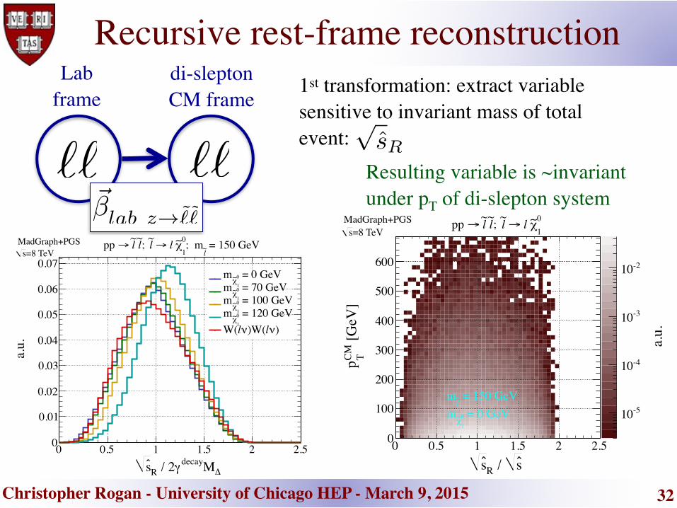
Lab frame
di-slepton CM frame
1st transformation: extract variable sensitive to invariant mass of total event:
Resulting variable is ~invariant under pT of di-slepton system
Recursive rest-frame reconstruction
32∆Mdecayγ / 2Rs
0 0.5 1 1.5 2 2.5
a.u.
0
0.01
0.02
0.03
0.04
0.05
0.06
0.07 = 0 GeV0
1χ∼
m = 70 GeV0
1χ∼
m = 100 GeV0
1χ∼
m = 120 GeV0
1χ∼
m)νl)W(νlW(
=8 TeVsMadGraph+PGS = 150 GeV
l~; m0
1χ∼ l → l~; l~ l~ →pp
s / Rs0 0.5 1 1.5 2 2.5
[GeV
]CM Tp
0
100
200
300
400
500
600
a.u.
-510
-410
-310
-210
=8 TeVsMadGraph+PGS
01χ∼ l → l~; l~ l~ →pp
= 0 GeV1
0χ∼
m = 150 GeVl~m
Christopher Rogan - University of Chicago HEP - March 9, 2015 33
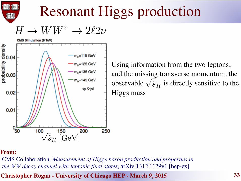
Resonant Higgs production
CMS Collaboration, Measurement of Higgs boson production and properties in the WW decay channel with leptonic final states, arXiv:1312.1129v1 [hep-ex]
From:
Using information from the two leptons, and the missing transverse momentum, the observable is directly sensitive to the Higgs mass

Christopher Rogan - University of Chicago HEP - March 9, 2015
di-slepton CM frame
slepton frameslepton frame
2nd transformation(s): extract variable sensitive to invariant mass of squark:
Resulting variable has kinematic endpoint at:
Recursive rest-frame reconstruction
34
[GeV]R∆M
0 50 100 150 200 250
[GeV
]CM Tp
0
50
100
150200
250
300
350400
450
a.u.
-510
-410
-310
=8 TeVsMadGraph+PGS ν±l → ±; W-W+ W→pp

Christopher Rogan - University of Chicago HEP - March 9, 2015
Variable comparison
35
More details about variable comparisons in PRD 89, 055020 (arXiv:1310.4827) and backup slides
∆ / MT2M0 0.2 0.4 0.6 0.8 1 1.2 1.4 1.6 1.8 2
a.u.
-510
-410
-310
-210
-110 = 0 GeV0
1χ∼
m = 70 GeV0
1χ∼
m = 100 GeV0
1χ∼
m = 120 GeV0
1χ∼
m
=8 TeVsMadGraph+PGS = 150 GeV
l~; m0
1χ∼ l → l~; l~ l~ →pp
∆ / MCTM0 0.2 0.4 0.6 0.8 1 1.2 1.4 1.6 1.8 2
a.u.
-510
-410
-310
-210
-110
1 = 0 GeV0
1χ∼
m = 70 GeV0
1χ∼
m = 100 GeV0
1χ∼
m = 120 GeV0
1χ∼
m
=8 TeVsMadGraph+PGS = 150 GeV
l~; m0
1χ∼ l → l~; l~ l~ →pp
∆ / MR∆M
0 0.2 0.4 0.6 0.8 1 1.2 1.4 1.6 1.8
a.u.
0
0.01
0.02
0.03
0.04
0.05
0.06 = 0 GeV0
1χ∼
m = 70 GeV0
1χ∼
m = 100 GeV0
1χ∼
m = 120 GeV0
1χ∼
m)νl)W(νlW(
=8 TeVsMadGraph+PGS = 150 GeV
l~; m0
1χ∼ l → l~; l~ l~ →pp
Three different singularity variables, all attempting to measure the same thing

Christopher Rogan - University of Chicago HEP - March 9, 2015
But what else can we calculate?
With recursive scheme can extract the two mass scales
and almost completely independently
36
∆Mtrueγ / 2Rs0 0.5 1 1.5 2 2.5
∆ /
MR ∆
M
00.20.40.60.8
11.21.41.61.8
2
a.u.
-510
-410
-310
=8 TeVsMadGraph+PGS
01χ∼ l → l~; l~ l~ →pp
= 50 GeV1
0χ∼
m = 150 GeVl~m
MR�
Christopher Rogan - University of Chicago HEP - March 9, 2015
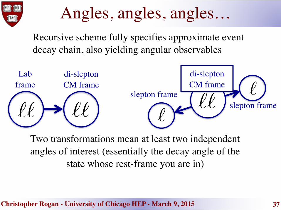
Angles, angles, angles…Recursive scheme fully specifies approximate event decay chain, also yielding angular observables
Two transformations mean at least two independent angles of interest (essentially the decay angle of the
state whose rest-frame you are in)
Lab frame
di-slepton CM frame
di-slepton CM frame
slepton frameslepton frame
37

Christopher Rogan - University of Chicago HEP - March 9, 2015
Towards a kinematic basis
but
while Underestimating the real mass means over-estimating the boost magnitude:
From PRD 89, 055020 (2014)38
s / Rs0 0.5 1 1.5 2 2.5
∆ /
MR ∆
M
00.20.40.60.8
11.21.41.61.8
2
a.u.
-510
-410
-310
=8 TeVsMadGraph+PGS
01χ∼ l → l~; l~ l~ →pp
= 0 GeV1
0χ∼
m = 150 GeVl~m
s / Rs0 0.5 1 1.5 2 2.5
∆ /
MR ∆
M0
0.20.40.60.8
11.21.41.61.8
2
a.u.
-510
-410
-310
=8 TeVsMadGraph+PGS
01χ∼ l → l~; l~ l~ →pp
= 50 GeV1
0χ∼
m = 150 GeVl~m
s / Rs0 0.5 1 1.5 2 2.5
∆ /
MR ∆
M
00.20.40.60.8
11.21.41.61.8
2
a.u.
-410
-310
-210=8 TeVs
MadGraph+PGS 01χ∼ l → l~; l~ l~ →pp
= 100 GeV1
0χ∼
m = 150 GeVl~m

Christopher Rogan - University of Chicago HEP - March 9, 2015
Towards a kinematic basis
but
while Underestimating the real mass means over-estimating the boost magnitude:
39TCMβ /
Rβ
0 0.5 1 1.5 2 2.5 3 3.5 4 4.5 5
a.u.
0
0.02
0.04
0.06
0.08
0.1 = 0 GeV0
1χ∼
m = 70 GeV0
1χ∼
m = 100 GeV0
1χ∼
m = 120 GeV0
1χ∼
m)νl)W(νlW(
=8 TeVsMadGraph+PGS = 150 GeV
l~; m0
1χ∼ l → l~; l~ l~ →pp
From PRD 89, 055020 (2014)
s / Rs0 0.5 1 1.5 2 2.5
∆ /
MR ∆
M
00.20.40.60.8
11.21.41.61.8
2
a.u.
-510
-410
-310
=8 TeVsMadGraph+PGS
01χ∼ l → l~; l~ l~ →pp
= 0 GeV1
0χ∼
m = 150 GeVl~m
s / Rs0 0.5 1 1.5 2 2.5
∆ /
MR ∆
M0
0.20.40.60.8
11.21.41.61.8
2
a.u.
-510
-410
-310
=8 TeVsMadGraph+PGS
01χ∼ l → l~; l~ l~ →pp
= 50 GeV1
0χ∼
m = 150 GeVl~m
s / Rs0 0.5 1 1.5 2 2.5
∆ /
MR ∆
M
00.20.40.60.8
11.21.41.61.8
2
a.u.
-410
-310
-210=8 TeVs
MadGraph+PGS 01χ∼ l → l~; l~ l~ →pp
= 100 GeV1
0χ∼
m = 150 GeVl~m
Christopher Rogan - University of Chicago HEP - March 9, 2015
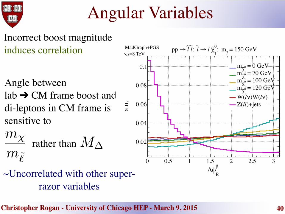
Angular Variables
Angle between lab ➔ CM frame boost and di-leptons in CM frame is sensitive to
rather than
Incorrect boost magnitude induces correlation
40
β
Rφ∆
0 0.5 1 1.5 2 2.5 3
a.u.
0.02
0.04
0.06
0.08
0.1 = 0 GeV0
1χ∼
m = 70 GeV0
1χ∼
m = 100 GeV0
1χ∼
m = 120 GeV0
1χ∼
m)νl)W(νlW(
)+jetsllZ(
=8 TeVsMadGraph+PGS = 150 GeV
l~; m0
1χ∼ l → l~; l~ l~ →pp
~Uncorrelated with other super-razor variables

Christopher Rogan - University of Chicago HEP - March 9, 2015
Angular Variables
In the approximate di-slepton rest frame, reconstructed decay angle sensitive to particle
spin and production
41
|R
θ| cos 0 0.1 0.2 0.3 0.4 0.5 0.6 0.7 0.8 0.9 1
a.u.
0
0.005
0.01
0.015
0.02
0.025
0.03
0.035
= 0 GeV0
1 χ
∼m
= 70 GeV0
1 χ
∼m
= 100 GeV0
1 χ
∼m
= 120 GeV0
1 χ
∼m
)νl)W(νlW(
=8 TeVsMadGraph+PGS = 150 GeV
l~; m
0
1 χ∼ l → l
~; l~ l~ →pp

Christopher Rogan - University of Chicago HEP - March 9, 2015
Angular Variables
In the approximate slepton rest frames, reconstructed slepton decay angle sensitive to
particle spin correlations
42
|R+1θ| cos 0 0.1 0.2 0.3 0.4 0.5 0.6 0.7 0.8 0.9 1
[G
eV]
R ∆M
0
20
40
60
80
100
0.001
0.002
0.003
0.004
0.005
0.006
0.007
0.008=8 TeVs
MadGraph+PGS ν±l → ±; W-W+ W→pp
|R+1θ| cos 0 0.1 0.2 0.3 0.4 0.5 0.6 0.7 0.8 0.9 1
[G
eV]
R ∆M
0
2040
60
80100
120
140160
180
0.0005
0.001
0.0015
0.002
0.0025
=8 TeVsMadGraph+PGS
01χ∼ l → l~; l~ l~ →pp
= 50 GeV1
0χ∼
m = 150 GeVl~m

Christopher Rogan - University of Chicago HEP - March 9, 2015
Angular Variables
Also allows us to better resolve the kinematic endpoint of interest
43
|R+1θ| cos 0 0.1 0.2 0.3 0.4 0.5 0.6 0.7 0.8 0.9 1
[G
eV]
R ∆M
0
2040
60
80100
120
140160
180
0.0005
0.001
0.0015
0.002
0.0025
=8 TeVsMadGraph+PGS
01χ∼ l → l~; l~ l~ →pp
= 50 GeV1
0χ∼
m = 150 GeVl~m
Christopher Rogan - University of Chicago HEP - March 9, 2015
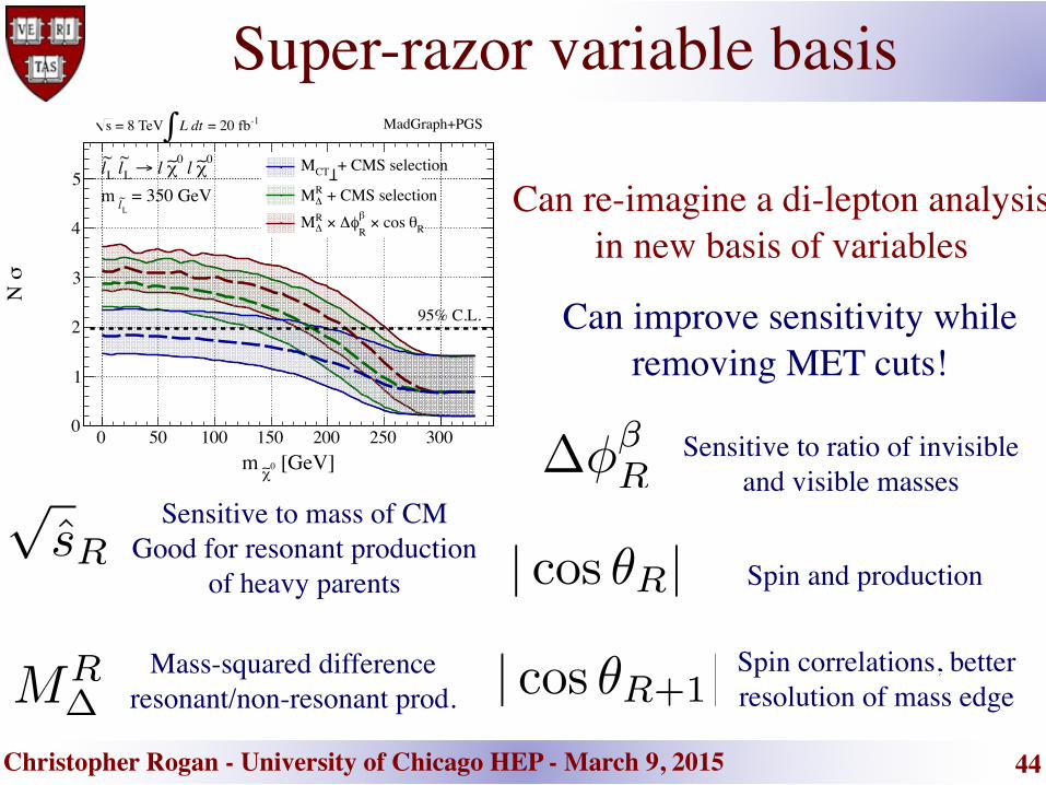
Super-razor variable basis
Sensitive to mass of CMGood for resonant production
of heavy parents
Mass-squared differenceresonant/non-resonant prod.
Sensitive to ratio of invisible and visible masses
Spin correlations, better resolution of mass edge
44
| cos ✓R| Spin and production
[GeV]0χ∼ m
0 50 100 150 200 250 300
σN
0
1
2
3
4
5 + CMS selectionCTM
+ CMS selection∆RM
Rθ cos × βRφ∆ × ∆RM
0χ∼ l 0
χ∼ l → Ll~ Ll
~
= 350 GeVLl
~ m
-1 = 20 fbL dt ∫ = 8 TeV s MadGraph+PGS
95% C.L. Can improve sensitivity while removing MET cuts!
Can re-imagine a di-lepton analysis in new basis of variables

Christopher Rogan - University of Chicago HEP - March 9, 2015 45
Generalizing further
Recursive Jigsaw approach can be generalized to arbitrarily complex final states with weakly interacting particles
Christopher Rogan - University of Chicago HEP - March 9, 2015
Christopher Rogan - University of Chicago HEP - March 9, 2015
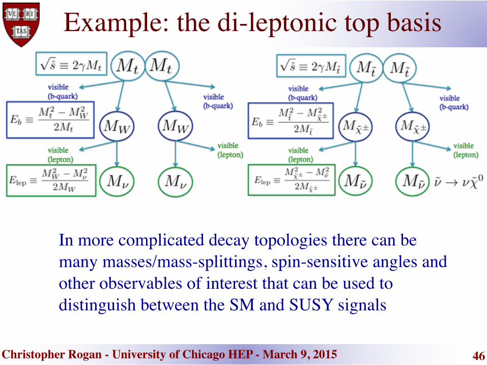
Example: the di-leptonic top basis
46
In more complicated decay topologies there can be many masses/mass-splittings, spin-sensitive angles and other observables of interest that can be used to distinguish between the SM and SUSY signals

Christopher Rogan - University of Chicago HEP - March 9, 2015 47
Singularity Variables for Tops
Christopher Rogan - University of Chicago HEP - March 9, 2015
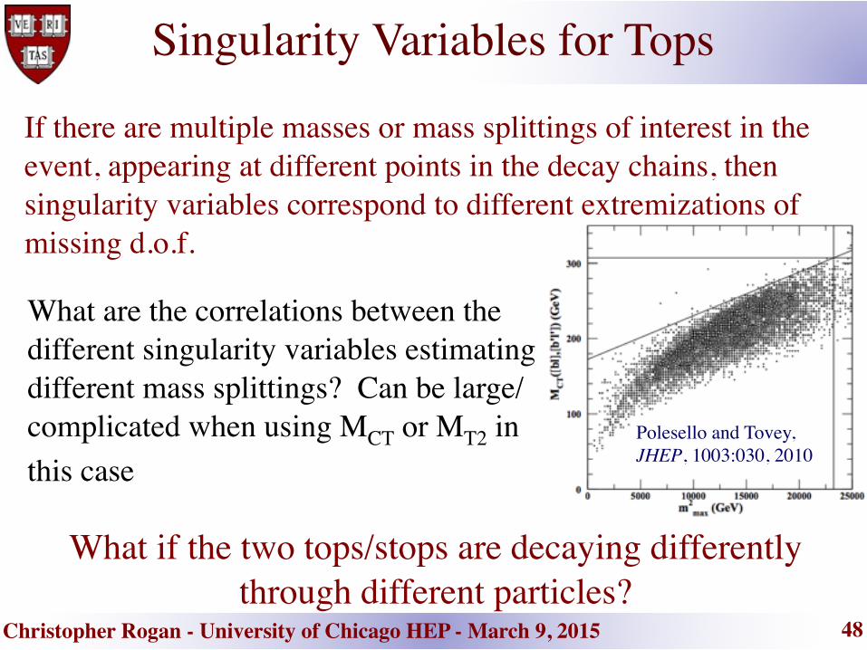
If there are multiple masses or mass splittings of interest in the event, appearing at different points in the decay chains, then singularity variables correspond to different extremizations of missing d.o.f.
What are the correlations between the different singularity variables estimating different mass splittings? Can be large/complicated when using MCT or MT2 in this case
What if the two tops/stops are decaying differently through different particles?
48
Singularity Variables for Tops
Polesello and Tovey, JHEP, 1003:030, 2010
Christopher Rogan - University of Chicago HEP - March 9, 2015 49
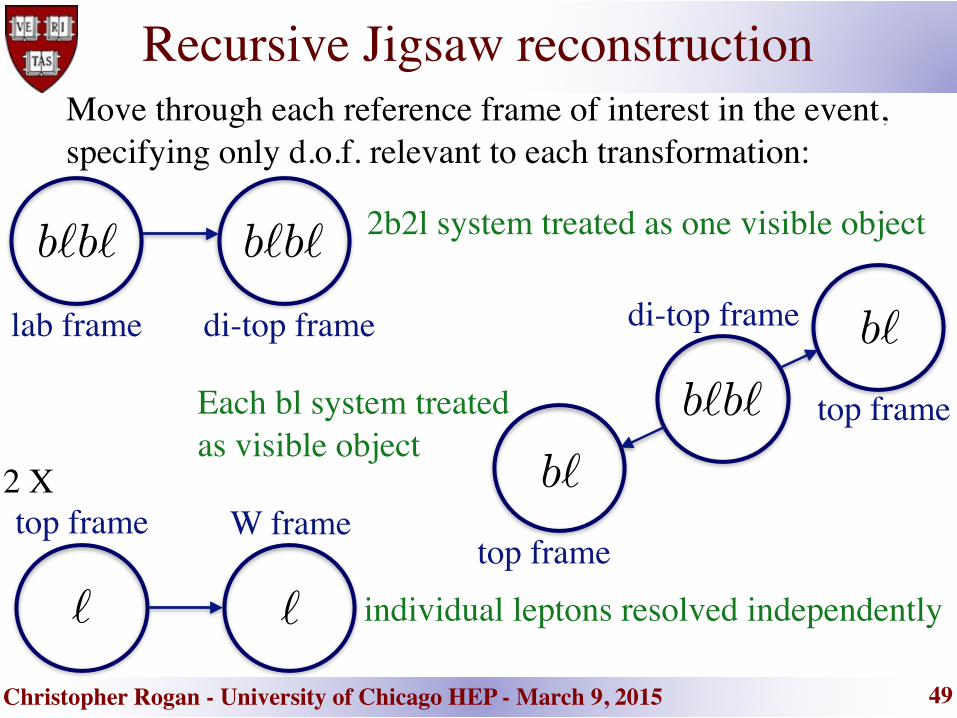
Recursive Jigsaw reconstructionMove through each reference frame of interest in the event, specifying only d.o.f. relevant to each transformation:
lab frame di-top frame di-top frame
top frame
top frame
top frame W frame
b`b` b`b`
b`b`
b`
b`
` `
2b2l system treated as one visible object
Each bl system treated as visible object
individual leptons resolved independently
2 X
Christopher Rogan - University of Chicago HEP - March 9, 2015 50
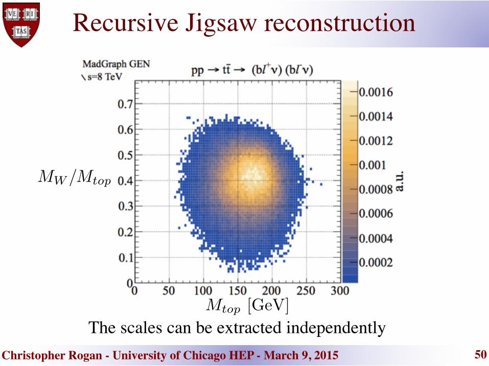
Recursive Jigsaw reconstruction
The scales can be extracted independently M
top
[GeV]
MW
/Mtop
Christopher Rogan - University of Chicago HEP - March 9, 2015 51
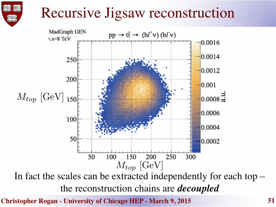
Recursive Jigsaw reconstruction
In fact the scales can be extracted independently for each top – the reconstruction chains are decoupled
Mtop
[GeV]
Mtop
[GeV]

Christopher Rogan - University of Chicago HEP - March 9, 2015 52
b-tagged jet
The di-leptonic top basis
b-tagged jet
lepton lepton
MET
2 X
a b��T1,T2
��T,W
Mtt̄, ~ptt̄, cos ✓TT
Etop�frame
b , cos ✓T
EW�frame` , cos ✓W

Christopher Rogan - University of Chicago HEP - March 9, 2015 53
The di-leptonic top basis
largely independent information about five different masses
true
b/ E
top-frame
b1E
0 0.2 0.4 0.6 0.8 1 1.2 1.4 1.6
true
b/ E
top-
fram
e
b2E
0
0.2
0.4
0.6
0.8
1
1.2
1.4
1.6
a.u.
0
0.001
0.002
0.003
0.004
0.005
0.006
0.007=8 TeVs
MadGraph GEN νl b→; t t t →pp
true
b/ E
top-frame
bE
0 0.2 0.4 0.6 0.8 1 1.2 1.4 1.6
true
l/ E
W-fr
ame
lE
0
0.2
0.4
0.6
0.8
1
1.2
1.4
1.6
a.u.
0
0.0005
0.001
0.0015
0.002
0.0025
0.003
0.0035
0.004=8 TeVs
MadGraph GEN νl b→; t t t →pp
true
l/ E
W-frame
1lE
0 0.2 0.4 0.6 0.8 1 1.2 1.4 1.6tru
e
l/ E
W-fr
ame
2lE
0
0.2
0.4
0.6
0.8
1
1.2
1.4
1.6
a.u.
0
0.0005
0.001
0.0015
0.002
0.0025
=8 TeVs
MadGraph GEN νl b→; t t t →pp
true
tt/ M
ttM
0 0.2 0.4 0.6 0.8 1 1.2 1.4 1.6
true
b/ E
top-
fram
e
bE
0
0.2
0.4
0.6
0.8
1
1.2
1.4
1.6
a.u.
0
0.001
0.002
0.003
0.004
0.005
0.006
0.007
0.008=8 TeVs
MadGraph GEN νl b→; t t t →pp
true
tt/ M
ttM
0 0.2 0.4 0.6 0.8 1 1.2 1.4 1.6
true
l/ E
W-fr
ame
lE
0
0.2
0.4
0.6
0.8
1
1.2
1.4
1.6
a.u.
00.00050.0010.00150.0020.00250.0030.00350.0040.0045
=8 TeVs
MadGraph GEN νl b→; t t t →pp

Christopher Rogan - University of Chicago HEP - March 9, 2015 54
Previous state-of-the-art
Mass-sensitive singularity variables are not necessarily independent
) [GeV]2
,b1
(bT2
M0 20 40 60 80 100 120 140 160
) [G
eV]
2l, 1l(T2
M
0
20
40
60
80
100
a.u.
-410
-310
-210
=8 TeVs
MadGraph GEN νl b→; t t t →pp
) [GeV]2l
2,b
1l
1(b
T2M
0 20 40 60 80 100 120 140 160 180
) [G
eV]
2,b 1
(bT2
M
0
20
40
60
80
100
120
140
160
a.u.
-410
-310
-210
=8 TeVs
MadGraph GEN νl b→; t t t →pp
) [GeV]2l
2,b
1l
1(b
T2M
0 20 40 60 80 100 120 140 160
) [G
eV]
2l, 1l(T2
M
0102030405060708090
a.u.
-410
-310
-210
=8 TeVs
MadGraph GEN νl b→; t t t →pp
Christopher Rogan - University of Chicago HEP - March 9, 2015 55
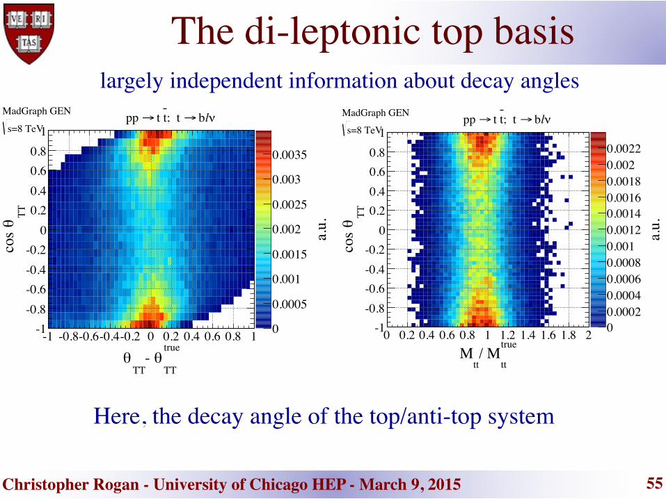
The di-leptonic top basis largely independent information about decay angles
true
TTθ-
TTθ
-1 -0.8-0.6-0.4-0.2 0 0.2 0.4 0.6 0.8 1
TTθ
cos
-1-0.8-0.6-0.4-0.2
00.20.40.60.8
1
a.u.0
0.0005
0.001
0.0015
0.002
0.0025
0.003
0.0035
=8 TeVs
MadGraph GEN νl b→; t t t →pp
true
tt/ M
ttM
0 0.2 0.4 0.6 0.8 1 1.2 1.4 1.6 1.8 2
TTθ
cos
-1-0.8-0.6-0.4-0.2
00.20.40.60.8
1
a.u.
00.00020.00040.00060.00080.0010.00120.00140.00160.00180.0020.0022
=8 TeVs
MadGraph GEN νl b→; t t t →pp
Here, the decay angle of the top/anti-top system

Christopher Rogan - University of Chicago HEP - March 9, 2015 56
The di-leptonic top basis
Here, the decay angle of one of the top quarks
true
b/ E
top-frame
bE
0 0.2 0.4 0.6 0.8 1 1.2 1.4 1.6T
θco
s -1
-0.8-0.6-0.4-0.2
00.20.40.60.8
1
a.u.
00.00020.00040.00060.00080.0010.00120.00140.00160.00180.002
=8 TeVs
MadGraph GEN νl b→; t t t →pp
true
Tθ-
Tθ
-1 -0.5 0 0.5 1
Tθ
cos
-1-0.8-0.6-0.4-0.2
00.20.40.60.8
1
a.u.
00.00020.00040.00060.00080.0010.00120.00140.00160.0018
=8 TeVs
MadGraph GEN νl b→; t t t →pp
largely independent information about decay angles
Christopher Rogan - University of Chicago HEP - March 9, 2015 57
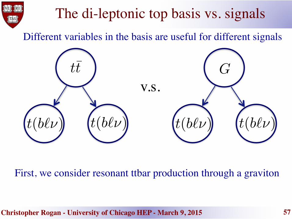
The di-leptonic top basis vs. signals Different variables in the basis are useful for different signals
First, we consider resonant ttbar production through a graviton
v.s.tt̄ G
t(b`⌫) t(b`⌫) t(b`⌫) t(b`⌫)

Christopher Rogan - University of Chicago HEP - March 9, 2015 58
The di-leptonic top basis vs. gravitons
Distributions of top/W/neutrino mass-splitting-sensitive observables are nearly identical since graviton signal and non-resonant background both contain on-shell tops
[GeV]top-frame
bE
0 20 40 60 80 100
a.u.
0
0.2
0.4
0.6
0.8
1 )ν l)(bν l (b→tt = 1 TeV
Gm
= 2 TeVG
m = 3 TeV
Gm
=8 TeVsMadGraph GEN νl b→; t t t → G →pp
[GeV]W-frame
lE
0 20 40 60 80 100
a.u.
0
0.2
0.4
0.6
0.8
1 )ν l)(bν l (b→tt = 1 TeV
Gm
= 2 TeVG
m = 3 TeV
Gm
=8 TeVsMadGraph GEN νl b→; t t t → G →pp
Different variables in the basis are useful for different signals

Christopher Rogan - University of Chicago HEP - March 9, 2015 59
The di-leptonic top basis vs. gravitons
Instead, observables related to the production of the two tops are sensitive to the intermediate resonance
[GeV]tt
M0 1000 2000 3000 4000 5000
a.u.
0
0.02
0.04
0.06
0.08
0.1
0.12
0.14
0.16
)ν l)(bν l (b→tt = 1 TeV
Gm
= 2 TeVG
m = 3 TeV
Gm
=8 TeVsMadGraph GEN νl b→; t t t → G →pp
TTθcos
-1 -0.8 -0.6 -0.4 -0.2 0 0.2 0.4 0.6 0.8 1
a.u.
0.2
0.4
0.6
0.8
1
)ν l)(bν l (b→tt = 1 TeV
Gm
= 2 TeVG
m = 3 TeV
Gm
=8 TeVsMadGraph GEN νl b→; t t t → G →pp
Different variables in the basis are useful for different signals
Christopher Rogan - University of Chicago HEP - March 9, 2015 60
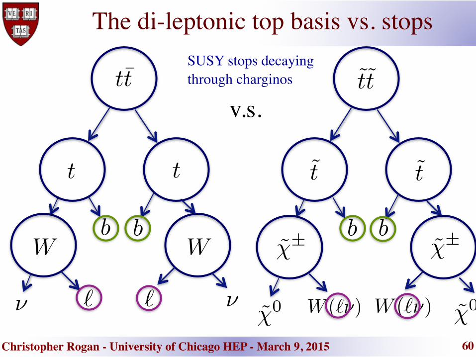
The di-leptonic top basis vs. stops SUSY stops decaying through charginos
v.s.tt̄ t̃t̃
t t t̃ t̃
b b b bW W �̃± �̃±
⌫ ⌫�̃0 �̃0` ` W (`⌫) W (`⌫)

Christopher Rogan - University of Chicago HEP - March 9, 2015 61
The di-leptonic top basis vs. stops
Mass-splitting-sensitive observables can be used to distinguish presence of signals
[GeV]top-frame
bE
0 50 100 150 200 250 300
a.u.
0.010.02
0.030.040.05
0.060.07
0.080.09
)ν l)(bν l (b→tt = 340 GeV
1
±
χ∼m
= 500 GeV1
±
χ∼m
= 650 GeV1
±
χ∼m
=8 TeVsMadGraph GEN
1
0 χ∼
) ν l W(→ 1
± χ∼
; 1
± χ∼
b → t~
; t~ t
~ →pp
= 300 GeV1
0χ∼m
= 700 GeVt~m
[GeV]W-frame
lE
0 20 40 60 80 100 120 140 160 180 200 220
a.u.
0.01
0.02
0.03
0.04
0.05
0.06
0.07
0.08)ν l)(bν l (b→tt
= 340 GeV1
±
χ∼m
= 500 GeV1
±
χ∼m
= 650 GeV1
±
χ∼m
=8 TeVsMadGraph GEN
1
0 χ∼
) ν l W(→ 1
± χ∼
; 1
± χ∼
b → t~
; t~ t
~ →pp
= 300 GeV1
0χ∼m
= 700 GeVt~m

Christopher Rogan - University of Chicago HEP - March 9, 2015 62
The di-leptonic top basis vs. stops mt̃ = 700 GeV
m�̃0 = 300 GeV
650500340
Here, the azimuthal angle between the the top and W decay planes and the angle between the two top decay planes
��T1,W1
��T1,T2T1,T2φ∆
0 1 2 3 4 5 6
T1,W
1φ
∆
0
1
2
3
4
5
6
a.u.
0.005
0.01
0.015
0.02
0.025
=8 TeVs
MadGraph GEN (300)1
0 χ∼
)νl W(→ 1
± χ∼
(340); 1
± χ∼
b→ t~
(700); t~ t
~ →pp
T1,T2φ∆
0 1 2 3 4 5 6
T1,W
1φ
∆
0
1
2
3
4
5
6
a.u.
0.0005
0.001
0.0015
0.002
0.0025
0.003
0.0035
=8 TeVs
MadGraph GEN (300)1
0 χ∼
)νl W(→ 1
± χ∼
(500); 1
± χ∼
b→ t~
(700); t~ t
~ →pp
T1,T2φ∆
0 1 2 3 4 5 6
T1,W
1φ
∆
0
1
2
3
4
5
6
a.u.
0.0006
0.0008
0.001
0.0012
0.0014
0.0016
0.0018
=8 TeVs
MadGraph GEN (300)1
0 χ∼
)νl W(→ 1
± χ∼
(650); 1
± χ∼
b→ t~
(700); t~ t
~ →pp
T1,T2φ∆
0 1 2 3 4 5 6
T1,W
1φ
∆
0
1
2
3
4
5
6
a.u.
0.0005
0.001
0.0015
0.002
0.0025=8 TeVs
MadGraph GEN νl b→; t t t →pp
m�̃± = GeV

Christopher Rogan - University of Chicago HEP - March 9, 2015
Summary▪ The strategy of Recursive Jigsaw Reconstruction is to not only
develop ‘good’ mass estimator variables, but to decompose each event into a basis of kinematic variables
▪ Through the recursive procedure, each variable is (as much as possible) independent of the others
▪ The interpretation of variables is straightforward; they each correspond to an actual, well-defined, quantity in the event
▪ Can be generalized to arbitrarily complex final states with many weakly interacting particles
▪ Code package to be released imminently (RestFrames - see back-up)▪ First papers nearing completion
(Recursive Jigsaw Reconstruction, The Di-leptonic ttbar basis - with Paul Jackson)
63

Christopher Rogan - University of Chicago HEP - March 9, 2015
▪ Recursive Jigsaw Reconstruction is a systematic recipe for deriving a kinematic basis for any open final state
▪ Mixed decay cases can now be treated in a sensible way
▪ Lots of potential applications – some I’m currently thinking about:• Di-lepton searches and differential measurements• stop / top-quark partner and resonant ttbar searches• other signatures (SUSY, exotica)• spin measurements• …
64
vs.vs.vs.
Outlook

Christopher Rogan - University of Chicago HEP - March 9, 2015
BACKUP SLIDES65

Christopher Rogan - University of Chicago HEP - March 9, 2015 66
RestFrames software library
RestFrames: Soon-to-be-public code that can be used to calculate kinematic variables associated with any decay chain and can implement “Recursive Jigsaw” rules
Example: Di-leptonic ttbar decays - how to use the code to initialize a decay tree, implement a jigsaw rule for determining the neutrino four-momenta, and analyze events
www.RestFrames.com

Christopher Rogan - University of Chicago HEP - March 9, 2015 67
initialize all your reference frames of interest
connect them according to the decay tree you want to impose on the event
RestFrames software library

Christopher Rogan - University of Chicago HEP - March 9, 2015 68
…and you’ll see this
draw your decay tree…
lab
tt
at
ab
aW
al
aν
bt
bb
bW
bl
bν
Lab State
Decay States
Visible States
Invisible States
RestFrames software library

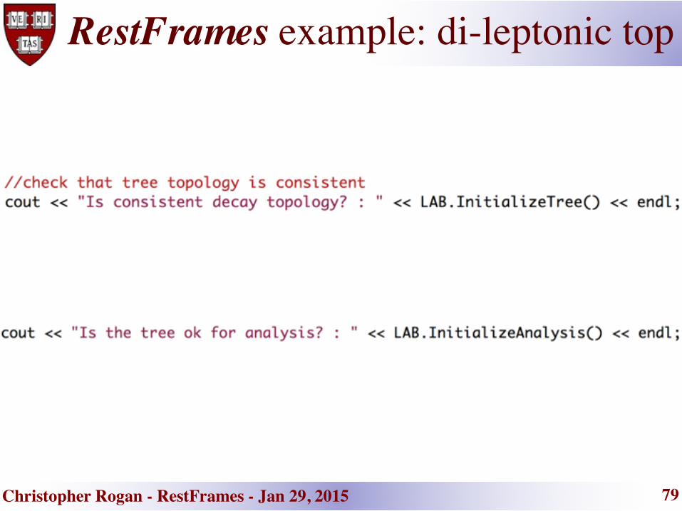
Christopher Rogan - RestFrames - Jan 29, 2015 69
RestFrames example: di-leptonic topSet the 4-vector input and MET for an event
Get observables directly from decay tree

Christopher Rogan - RestFrames - Jan 29, 2015 70
tt
at
ab
aW
al
aν
bt
bb
bW
bl
bν
Decay States
Visible States
Invisible States at
ab
aW
al
aν
Decay States
Visible States
Invisible States
RestFrames example: di-leptonic top

Christopher Rogan - RestFrames - Jan 29, 2015 71
RestFrames example: di-leptonic top

Christopher Rogan - RestFrames - Jan 29, 2015 72
number of elements that _have_ to go to this frame from the group each event exclusive (true) or
inclusive (false) counting
RestFrames example: di-leptonic top

Christopher Rogan - RestFrames - Jan 29, 2015 73
RestFrames example: di-leptonic top

Christopher Rogan - RestFrames - Jan 29, 2015 74
tt
at
ab
aW
al
aν
bt
bb
bW
bl
bν
tt
at
ab
aW
al
aν
bt
bb
bW
bl
bν
Decay States
Visible States
Invisible States
Invisible Jigsaw
RestFrames example: di-leptonic top

Christopher Rogan - RestFrames - Jan 29, 2015 75
event-by-event will choose b-tag jet combinatoric assignment that minimizes the masses of these two collections
RestFrames example: di-leptonic top

Christopher Rogan - RestFrames - Jan 29, 2015 76
tt
at
ab
aW
al
aν
bt
bb
bW
bl
bν
tt
at
ab
aW
al
aν
bt
bb
bW
bl
bν
Decay States
Visible States
Invisible States
Invisible Jigsaw
Combinatoric Jigsaw
RestFrames example: di-leptonic top

Christopher Rogan - RestFrames - Jan 29, 2015 77
Invisible system mass Jigsaw
Invisible system rapidity Jigsaw
Contraboost invariant JigsawContraboost invariant Jigsaw
bν+
aν
bν+
aν
bν+
aν
aν
bν
Invisible Frame Jigsaws
RestFrames example: di-leptonic top
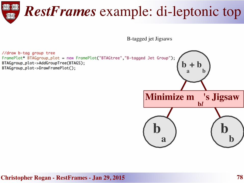
Christopher Rogan - RestFrames - Jan 29, 2015 78
's Jigsawlb
Minimize m 's Jigsawlb
Minimize m
b+ b
ab
ab
bb
B-tagged jet Jigsaws
RestFrames example: di-leptonic top
Christopher Rogan - RestFrames - Jan 29, 2015 79
RestFrames example: di-leptonic top

Christopher Rogan - RestFrames - Jan 29, 2015 80
some toy input
analyze the event
RestFrames example: di-leptonic top

Christopher Rogan - RestFrames - Jan 29, 2015 81
tracking of combinatoric elements
RestFrames example: di-leptonic top

Christopher Rogan - RestFrames - Jan 29, 2015
▪ To make shared library ‘lib/libRestFrames.so’
▪ To set environmental variables (ex. for running ROOT macros):
82
RestFrames setup
<$ make
<$ source setup.sh

Christopher Rogan - RestFrames - Jan 29, 2015
▪ To run ‘macros/TestDiLeptonicTop.C’ macro:
83
<$ root
root [0] .x macros/TestDiLeptonicTop.C
RestFrames example: di-leptonic top

Christopher Rogan - University of Chicago HEP - March 9, 2015
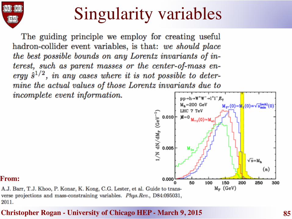
Singularity variables
From:
84
Christopher Rogan - University of Chicago HEP - March 9, 2015
Singularity variables
From:
85

Christopher Rogan - University of Chicago HEP - March 9, 2015
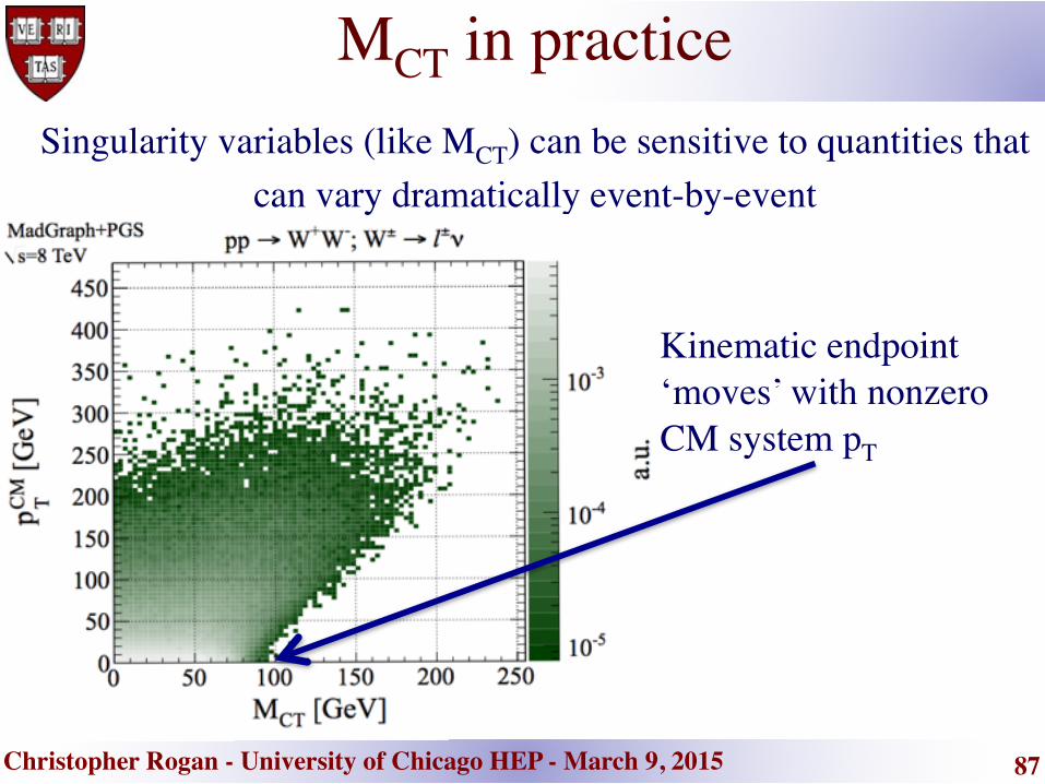
Example: MCT
Constructed to have a kinematic endpoint at:
From:
assuming ~mass-less leptons
86
Christopher Rogan - University of Chicago HEP - March 9, 2015
MCT in practiceSingularity variables (like MCT) can be sensitive to quantities that
can vary dramatically event-by-event
Kinematic endpoint ‘moves’ with nonzero CM system pT
87

Christopher Rogan - University of Chicago HEP - March 9, 2015
The mass challengeThe invariant mass is invariant under coherent Lorentz transformations of two particles
The Euclidean mass (or contra-variant mass) is invariant under anti-symmetric Lorentz transformations of two particles
Even the simplest case requires variables with both properties!Lab
framedi-slepton CM frame
di-slepton CM frame
slepton frameslepton frame
88

Christopher Rogan - University of Chicago HEP - March 9, 2015
Correcting for CM pT
▪ Want to boost from lab-frame to CM-frame▪ We know the transverse momentum of the CM-
frame:
▪ But we don’t know the energy, or mass, of the CM-frame:
89

Christopher Rogan - University of Chicago HEP - March 9, 2015
pT corrections for MCT
with:
Attempts have been made to mitigate this problem:(i) ‘Guess’ the lab ➔ CM frame boost:
(ii) Only look at event along axis perpendicular to boost:
x – parallel to boosty – perp. to boost
90
Christopher Rogan - University of Chicago HEP - March 9, 2015
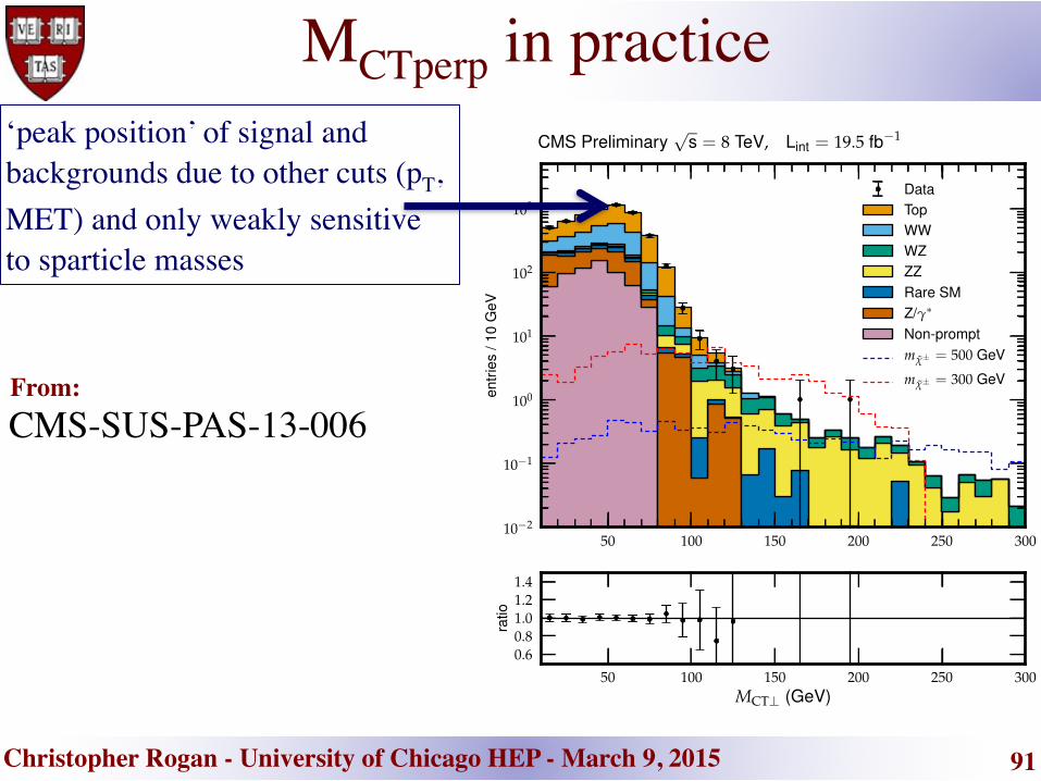
MCTperp in practice
CMS-SUS-PAS-13-006
‘peak position’ of signal and backgrounds due to other cuts (pT, MET) and only weakly sensitive to sparticle masses
From:
91
50 100 150 200 250 30010�2
10�1
100
101
102
103
entri
es/1
0G
eV
DataTopWWWZZZRare SMZ/g⇤
Non-promptm
c̃
± = 500 GeV
mc̃
± = 300 GeV
50 100 150 200 250 300MCT? (GeV)
0.60.81.01.21.4
ratio
CMS Preliminaryp
s = 8 TeV, Lint = 19.5 fb�1
Christopher Rogan - University of Chicago HEP - March 9, 2015
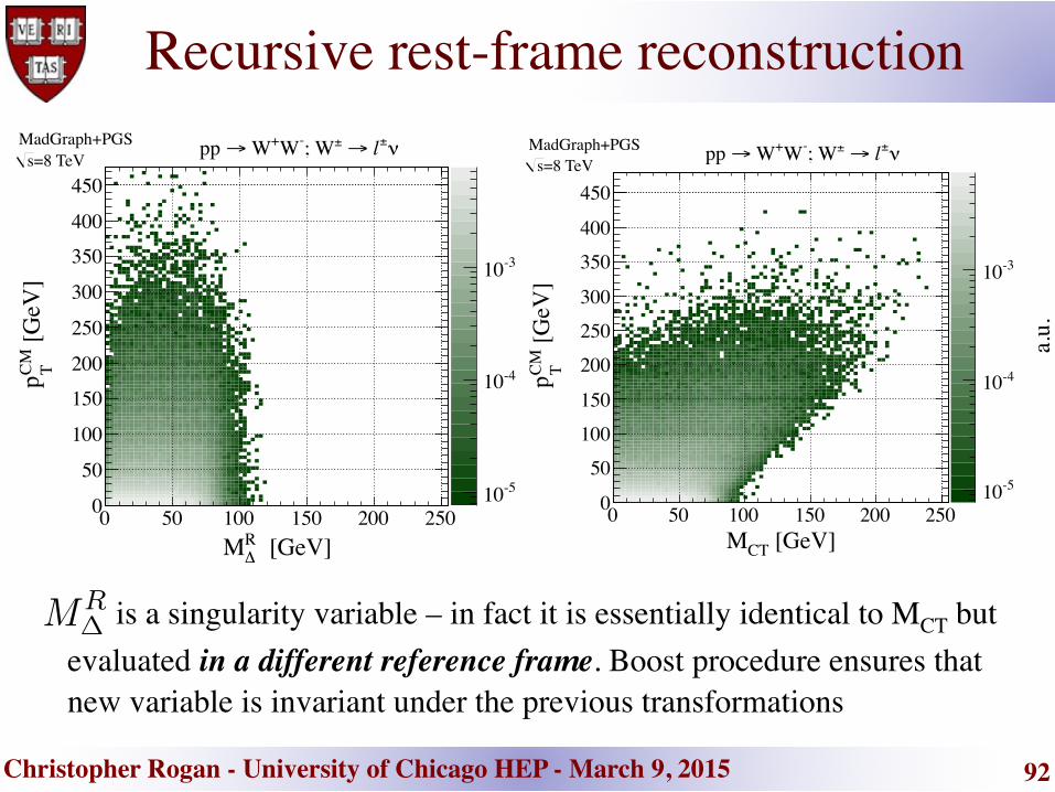
is a singularity variable – in fact it is essentially identical to MCT but evaluated in a different reference frame. Boost procedure ensures that new variable is invariant under the previous transformations
Recursive rest-frame reconstruction
92
[GeV]R∆M
0 50 100 150 200 250
[GeV
]CM Tp
0
50
100
150200
250
300
350400
450
a.u.
-510
-410
-310
=8 TeVsMadGraph+PGS ν±l → ±; W-W+ W→pp
[GeV]CTM0 50 100 150 200 250
[GeV
]CM Tp
0
50100150
200250300
350400
450
a.u.
-510
-410
-310
=8 TeVsMadGraph+PGS ν±l → ±; W-W+ W→pp

Christopher Rogan - University of Chicago HEP - March 9, 2015 93
Resonant Higgs production
CMS Collaboration, Measurement of Higgs boson production and properties in the WW decay channel with leptonic final states, arXiv:1312.1129v1 [hep-ex]
From:
The between the leptons is evaluated in the R-frame, removing dependence on the pT of the Higgs and correlation with
CMS uses 2D fit of variables to measure Higgs mass in this channel

Christopher Rogan - University of Chicago HEP - March 9, 2015 94
Resonant Higgs production
CMS Collaboration, Measurement of Higgs boson production and properties in the WW decay channel with leptonic final states, arXiv:1312.1129v1 [hep-ex]
From:
The shape of the distribution, for the Higgs signal and backgrounds, is used to extract both the Higgs mass and signal strength – even while information is lost with the two escaping neutrinos

Christopher Rogan - University of Chicago HEP - March 9, 2015
What other info can we extract?
Mass and Spin Measurement with M(T2) and MAOS Momentum - Cho, Won Sang et al. Nucl.Phys.Proc.Suppl. 200-202 (2010) 103-112 arXiv:0909.4853 [hep-ph]
From:
Ex. MT2 extremization assigns values to missing degrees of freedom – if one takes
these assignments literally, can we calculate other useful variables?
When we assign unconstrained d.o.f. by extremizing one quantity, what are the general properties of other variables we calculate? What are the correlations among them?
95

Christopher Rogan - University of Chicago HEP - March 9, 2015
Example: the di-leptonic top basis
96
[GeV]top-frame
bE
-1 -0.8 -0.6 -0.4 -0.2 0 0.2 0.4 0.6 0.8 1
a.u.
0
0.005
0.01
0.015
0.02
0.025
0.03
0.035
)ν l)(bν l (b→tt = 340 GeV
1
±
χ∼m
= 500 GeV1
±
χ∼m
= 650 GeV1
±
χ∼m
=8 TeVsMadGraph GEN
1
0χ∼
) νl W(→ 1
±
χ∼
; 1
±
χ∼
b → t~
; t~ t
~ →pp
= 300 GeV1
0χ∼m
= 700 GeVt~m
[GeV]tt
M0 1000 2000 3000 4000 5000
a.u.
0
0.02
0.04
0.06
0.08
0.1
0.12
0.14
0.16
)ν l)(bν l (b→tt = 1 TeV
Gm
= 2 TeVG
m = 3 TeV
Gm
=8 TeVsMadGraph GEN νl b→; t t t → G →pp
true
tt/ M
ttM
0 0.2 0.4 0.6 0.8 1 1.2 1.4 1.6 1.8 2
TTθ
cos
-1-0.8-0.6-0.4-0.2
00.20.40.60.8
1
a.u.
00.00020.00040.00060.00080.0010.00120.00140.00160.00180.0020.0022
=8 TeVs
MadGraph GEN νl b→; t t t →pp
A rich basis of useful Recursive Jigsaw observables can be calculated, each with largely independent information
true
b/ E
top-frame
bE
0 0.2 0.4 0.6 0.8 1 1.2 1.4 1.6
true
l/ E
W-fr
ame
lE
0
0.2
0.4
0.6
0.8
1
1.2
1.4
1.6
a.u.
0
0.0005
0.001
0.0015
0.002
0.0025
0.003
0.0035
0.004=8 TeVs
MadGraph GEN νl b→; t t t →pp
true
b/ E
top-frame
b1E
0 0.2 0.4 0.6 0.8 1 1.2 1.4 1.6
true
b/ E
top-
fram
e
b2E
0
0.2
0.4
0.6
0.8
1
1.2
1.4
1.6
a.u.
0
0.001
0.002
0.003
0.004
0.005
0.006
0.007=8 TeVs
MadGraph GEN νl b→; t t t →pp
true
tt/ M
ttM
0 0.2 0.4 0.6 0.8 1 1.2 1.4 1.6
true
b/ E
top-
fram
e
bE
0
0.2
0.4
0.6
0.8
1
1.2
1.4
1.6
a.u.
0
0.001
0.002
0.003
0.004
0.005
0.006
0.007
0.008=8 TeVs
MadGraph GEN νl b→; t t t →pp
true
tt/ M
ttM
0 0.2 0.4 0.6 0.8 1 1.2 1.4 1.6
true
l/ E
W-fr
ame
lE
0
0.2
0.4
0.6
0.8
1
1.2
1.4
1.6
a.u.
00.00050.0010.00150.0020.00250.0030.00350.0040.0045
=8 TeVs
MadGraph GEN νl b→; t t t →pp
true
l/ E
W-frame
1lE
0 0.2 0.4 0.6 0.8 1 1.2 1.4 1.6
true
l/ E
W-fr
ame
2lE
0
0.2
0.4
0.6
0.8
1
1.2
1.4
1.6
a.u.
0
0.0005
0.001
0.0015
0.002
0.0025
=8 TeVs
MadGraph GEN νl b→; t t t →pp

Christopher Rogan - University of Chicago HEP - March 9, 2015 97
The di-leptonic top basis vs. stops
Observables sensitive to intermediate resonances cannot distinguish between non-resonant signals and background
Tγ
1 2 3 4 5 6 7 8
a.u.
-410
-310
-210
)ν l)(bν l (b→tt = 1 TeV
Gm
= 2 TeVG
m = 3 TeV
Gm
=8 TeVsMadGraph GEN νl b→; t t t → G →pp
Tγ
1 2 3 4 5 6
a.u.
-310
-210
-110 )ν l)(bν l (b→tt
= 340 GeV1
±
χ∼m
= 500 GeV1
±
χ∼m
= 650 GeV1
±
χ∼m
=8 TeVsMadGraph GEN
1
0χ∼
) νl W(→ 1
±
χ∼
; 1
±
χ∼
b → t~
; t~ t
~ →pp
= 300 GeV1
0χ∼m
= 700 GeVt~m
Mtt = 2�TMt

Christopher Rogan - University of Chicago HEP - March 9, 2015
vs.
Mul
ti-di
men
siona
l bum
p-hu
ntin
g
98
MW
/Mtop
MW
/Mtop
Mtop
[GeV]
Mtop
[GeV] Mtop
[GeV]
Mtop
[GeV]M
W
/Mtop
MW
/Mtop
Christopher Rogan - University of Chicago HEP - March 9, 2015 99
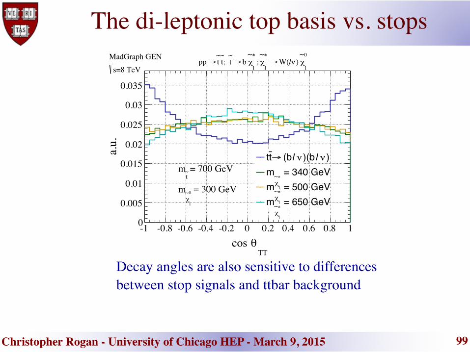
The di-leptonic top basis vs. stops
Decay angles are also sensitive to differences between stop signals and ttbar background
[GeV]top-frame
bE
-1 -0.8 -0.6 -0.4 -0.2 0 0.2 0.4 0.6 0.8 1
a.u.
0
0.005
0.01
0.015
0.02
0.025
0.03
0.035
)ν l)(bν l (b→tt = 340 GeV
1
±
χ∼m
= 500 GeV1
±
χ∼m
= 650 GeV1
±
χ∼m
=8 TeVsMadGraph GEN
1
0χ∼
) νl W(→ 1
±
χ∼
; 1
±
χ∼
b → t~
; t~ t
~ →pp
= 300 GeV1
0χ∼m
= 700 GeVt~m
TTθcos
-1 -0.8 -0.6 -0.4 -0.2 0 0.2 0.4 0.6 0.8 1
a.u.
0.2
0.4
0.6
0.8
1
)ν l)(bν l (b→tt = 1 TeV
Gm
= 2 TeVG
m = 3 TeV
Gm
=8 TeVsMadGraph GEN νl b→; t t t → G →pp
Christopher Rogan - University of Chicago HEP - March 9, 2015 100
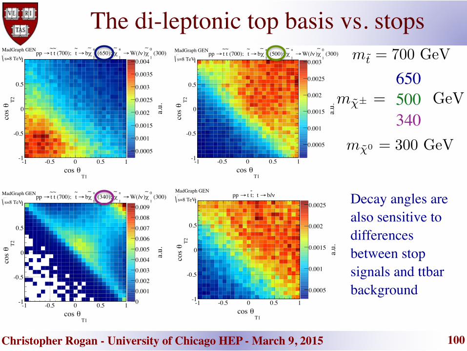
The di-leptonic top basis vs. stops mt̃ = 700 GeV
m�̃0 = 300 GeV
650500340
Decay angles are also sensitive to differences between stop signals and ttbar background
T1θcos
-1 -0.5 0 0.5 1
T2θ
cos
-1
-0.5
0
0.5
1
a.u.
00.0010.0020.0030.0040.0050.0060.0070.0080.009
=8 TeVs
MadGraph GEN (300)1
0 χ∼
)νl W(→ 1
± χ∼
(340); 1
± χ∼
b→ t~
(700); t~ t
~ →pp
T1θcos
-1 -0.5 0 0.5 1
T2θ
cos
-1
-0.5
0
0.5
1
a.u.
0.0005
0.001
0.0015
0.002
0.0025
0.003=8 TeVs
MadGraph GEN (300)1
0 χ∼
)νl W(→ 1
± χ∼
(500); 1
± χ∼
b→ t~
(700); t~ t
~ →pp
T1θcos
-1 -0.5 0 0.5 1
T2θ
cos
-1
-0.5
0
0.5
1
a.u.
0.0005
0.001
0.0015
0.002
0.0025
0.003
0.0035
0.004=8 TeVs
MadGraph GEN (300)1
0 χ∼
)νl W(→ 1
± χ∼
(650); 1
± χ∼
b→ t~
(700); t~ t
~ →pp
T1θcos
-1 -0.5 0 0.5 1
T2θ
cos
-1
-0.5
0
0.5
1
a.u.
0.0005
0.001
0.0015
0.002
0.0025=8 TeVs
MadGraph GEN νl b→; t t t →pp
m�̃± = GeV
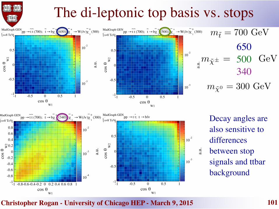
Christopher Rogan - University of Chicago HEP - March 9, 2015 101
The di-leptonic top basis vs. stops mt̃ = 700 GeV
m�̃0 = 300 GeV
650500340
Decay angles are also sensitive to differences between stop signals and ttbar background
W1θcos
-1 -0.8-0.6-0.4-0.2 0 0.2 0.4 0.6 0.8 1
W2
θco
s
-1-0.8-0.6-0.4-0.2
00.20.40.60.8
1
a.u.
-410
-310
-210
=8 TeVs
MadGraph GEN (300)1
0 χ∼
)νl W(→ 1
± χ∼
(340); 1
± χ∼
b→ t~
(700); t~ t
~ →pp
W1θcos
-1 -0.5 0 0.5 1
W2
θco
s
-1
-0.5
0
0.5
1
a.u.
-310
-210
=8 TeVs
MadGraph GEN (300)1
0 χ∼
)νl W(→ 1
± χ∼
(500); 1
± χ∼
b→ t~
(700); t~ t
~ →pp
W1θcos
-1 -0.5 0 0.5 1
W2
θco
s
-1
-0.5
0
0.5
1
a.u.
-310
-210
=8 TeVs
MadGraph GEN (300)1
0 χ∼
)νl W(→ 1
± χ∼
(650); 1
± χ∼
b→ t~
(700); t~ t
~ →pp
W1θcos
-1 -0.5 0 0.5 1
W2
θco
s
-1
-0.5
0
0.5
1
a.u.
-310
-210
=8 TeVs
MadGraph GEN νl b→; t t t →pp
m�̃± = GeV

Christopher Rogan - University of Chicago HEP - March 9, 2015 102
The di-leptonic top basis vs. stops mt̃ = 700 GeV
m�̃0 = 300 GeV
650500340
Here, the azimuthal angle between the the top and W decay planes , for each of the two decay chains
��T1,W1
T1,W1φ∆
0 1 2 3 4 5 6
T2,W
2φ
∆
0
1
2
3
4
5
6
a.u.
0.001
0.002
0.003
0.004
0.005
0.006
0.007=8 TeVs
MadGraph GEN (300)1
0 χ∼
)νl W(→ 1
± χ∼
(340); 1
± χ∼
b→ t~
(700); t~ t
~ →pp
T1,W1φ∆
0 1 2 3 4 5 6
T2,W
2φ
∆
0
1
2
3
4
5
6
a.u.
0.0005
0.001
0.0015
0.002
0.0025
=8 TeVs
MadGraph GEN (300)1
0 χ∼
)νl W(→ 1
± χ∼
(500); 1
± χ∼
b→ t~
(700); t~ t
~ →pp
T1,W1φ∆
0 1 2 3 4 5 6
T2,W
2φ
∆
0
1
2
3
4
5
6
a.u.
0.0005
0.001
0.0015
0.002
0.0025
0.003
=8 TeVs
MadGraph GEN (300)1
0 χ∼
)νl W(→ 1
± χ∼
(650); 1
± χ∼
b→ t~
(700); t~ t
~ →pp
T1,W1φ∆
0 1 2 3 4 5 6
T2,W
2φ
∆
0
1
2
3
4
5
6
a.u.
0.0005
0.001
0.0015
0.002
0.0025
0.003
=8 TeVs
MadGraph GEN νl b→; t t t →pp
m�̃± = GeV

Christopher Rogan - University of Chicago HEP - March 9, 2015 103
The di-leptonic top basis vs. stops mt̃ = 700 GeV
m�̃0 = 300 GeV
650500340
Here, the azimuthal angle between the the top and W decay planes and the angle between the two top decay planes
��T1,W1
��T1,T2T1,T2φ∆
0 1 2 3 4 5 6
T1,W
1φ
∆
0
1
2
3
4
5
6
a.u.
0.005
0.01
0.015
0.02
0.025
=8 TeVs
MadGraph GEN (300)1
0 χ∼
)νl W(→ 1
± χ∼
(340); 1
± χ∼
b→ t~
(700); t~ t
~ →pp
T1,T2φ∆
0 1 2 3 4 5 6
T1,W
1φ
∆
0
1
2
3
4
5
6
a.u.
0.0005
0.001
0.0015
0.002
0.0025
0.003
0.0035
=8 TeVs
MadGraph GEN (300)1
0 χ∼
)νl W(→ 1
± χ∼
(500); 1
± χ∼
b→ t~
(700); t~ t
~ →pp
T1,T2φ∆
0 1 2 3 4 5 6
T1,W
1φ
∆
0
1
2
3
4
5
6
a.u.
0.0006
0.0008
0.001
0.0012
0.0014
0.0016
0.0018
=8 TeVs
MadGraph GEN (300)1
0 χ∼
)νl W(→ 1
± χ∼
(650); 1
± χ∼
b→ t~
(700); t~ t
~ →pp
T1,T2φ∆
0 1 2 3 4 5 6
T1,W
1φ
∆
0
1
2
3
4
5
6
a.u.
0.0005
0.001
0.0015
0.002
0.0025=8 TeVs
MadGraph GEN νl b→; t t t →pp
m�̃± = GeV

Christopher Rogan - University of Chicago HEP - March 9, 2015
Razor kinematic variablesmega-jet
invisible?▪ Assign every reconstructed object to one of two mega-jets▪ Analyze the event as a ‘canonical’ open final state:
• two variables: MR (mass scale) , R (scale-less event imbalance)
▪ An inclusive approach to searching for a large class of new physics possibilities with open final states
invisible?
mega-jet
PRD 85, 012004 (2012)EPJC 73, 2362 (2013)PRL 111, 081802 (2013)CMS-PAS-SUS-13-004
arXiv:1006.2727v1 [hep-ph]Razor variables
CMS+ATLASanalyses
104Christopher Rogan - University of Chicago HEP - March 9, 2015

Christopher Rogan - University of Chicago HEP - March 9, 2015
Razor kinematic variablesmega-jet
invisible?▪ Assign every reconstructed object to one of two mega-jets▪ Analyze the event as a ‘canonical’ open final state:
• two variables: MR (mass scale) , R (scale-less event imbalance)
▪ An inclusive approach to searching for a large class of new physics possibilities with open final states
invisible?
mega-jet
Two distinct mass scales in event Two pieces of complementary information
105Christopher Rogan - University of Chicago HEP - March 9, 2015
Christopher Rogan - University of Chicago HEP - March 9, 2015
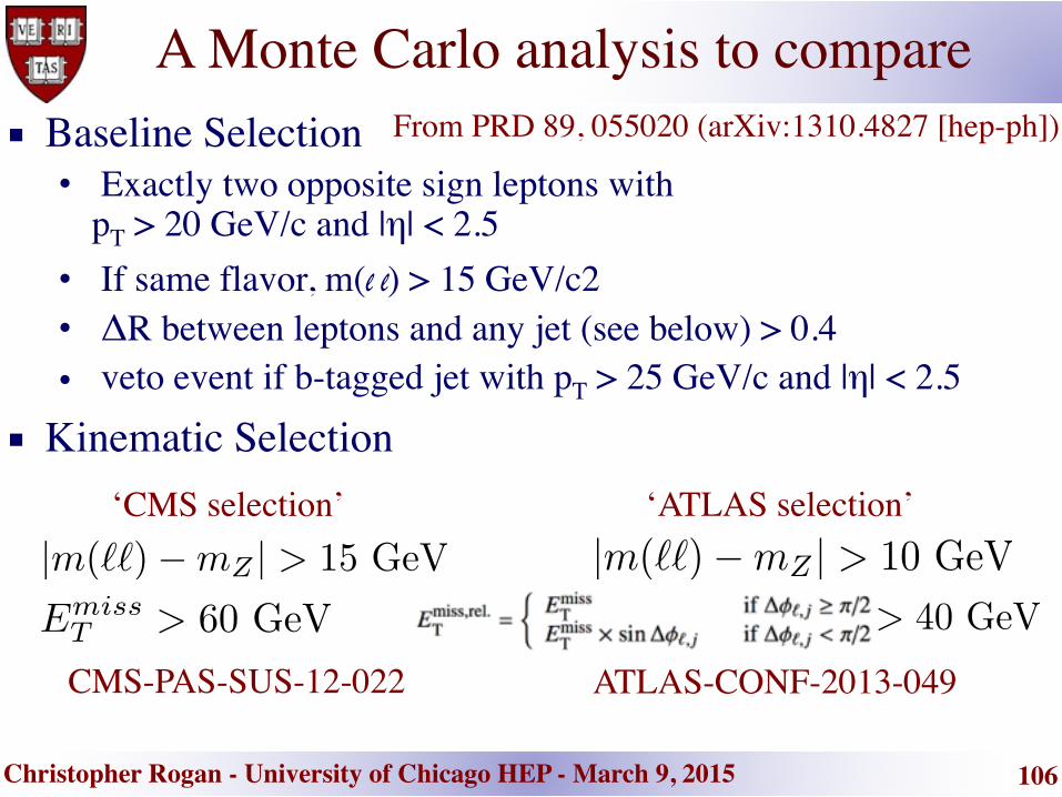
▪ Baseline Selection• Exactly two opposite sign leptons with
pT > 20 GeV/c and |η| < 2.5• If same flavor, m(l l) > 15 GeV/c2• ΔR between leptons and any jet (see below) > 0.4• veto event if b-tagged jet with pT > 25 GeV/c and |η| < 2.5
▪ Kinematic Selection
ATLAS-CONF-2013-049CMS-PAS-SUS-12-022
‘CMS selection’ ‘ATLAS selection’
A Monte Carlo analysis to compareFrom PRD 89, 055020 (arXiv:1310.4827 [hep-ph])
106
Christopher Rogan - University of Chicago HEP - March 9, 2015
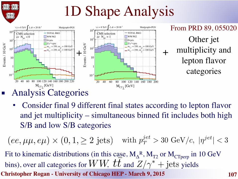
1D Shape Analysis
▪ Analysis Categories • Consider final 9 different final states according to lepton flavor
and jet multiplicity – simultaneous binned fit includes both high S/B and low S/B categories
Fit to kinematic distributions (in this case, MΔR, MT2 or MCTperp in 10 GeV
bins), over all categories for , and yields
Other jet multiplicity and
lepton flavor categories
+
107
[GeV] CTM20 40 60 80 100 120 140 160 180 200 220
Even
ts / 1
0 G
eV
-110
1
10
210
310
410 TOTAL BKGWW/WZ
+jetstt*+jetsγZ/
= 100 GeV0χ∼
= 350, m±Le~m
= 100 GeV0χ∼
= 250, m±Le~m
-1 = 20 fbL dt ∫ = 8 TeV s Madgraph+PGS
= 0jet NeeCMS selection
[GeV] CTM20 40 60 80 100 120 140 160 180 200
Even
ts / 1
0 G
eV
-110
1
10
210
310
410TOTAL BKGWW/WZ
+jetstt*+jetsγZ/
= 100 GeV0χ∼
= 350, m±Le~m
= 100 GeV0χ∼
= 250, m±Le~m
-1 = 20 fbL dt ∫ = 8 TeV s Madgraph+PGS
= 1jet NeeCMS selection
+
From PRD 89, 055020

Christopher Rogan - University of Chicago HEP - March 9, 2015
Systematic uncertainties
▪ 2% lepton ID (correlated btw bkgs, uncorrelated between lepton categories)
▪ 10% jet counting (per jet) (uncorrelated between all processes)▪ 10% x-section uncertainty for backgrounds (uncorrelated) +
theoretical x-section uncertainty for signal (small)▪ ‘shape’ uncertainty derived by propagating effect of 10% jet
energy scale shift up/down to MET and recalculating shapes templates of kinematic variables
▪ Uncertainties are introduced into toy pseudo-experiments through marginalization (pdfs fixed in likelihood evaluation but systematically varied in shape and normalization in toy pseudo-experiment generation)
108
From PRD 89, 055020 (arXiv:1310.4827 [hep-ph])

Christopher Rogan - University of Chicago HEP - March 9, 2015
Compared to Reality
(GeV)l~
m100 150 200 250 300 350 400 450
(G
eV)
0 1χ∼m
0
50
100
150
200
250
300
95%
C.L
. upp
er lim
it on
cro
ss s
ectio
n (fb
)
1
10
210 = 8 TeVs, -1 = 19.5 fb
intCMS Preliminary L
95% C.L. CLs NLO Exclusions
theoryσ 1±Observed
experimentσ1±Expected
Lµ∼
Lµ∼, Le
~ Le~ → pp
) = 101χ∼ l → Ll
~(Br
CMS-PAS-SUS-12-022
109
From PRD 89, 055020 (arXiv:1310.4827 [hep-ph])

Christopher Rogan - University of Chicago HEP - March 9, 2015
Expected Limit Comparison
110
[GeV]Ll~m
100 150 200 250 300 350 400 450
[GeV
]0 χ∼
m
0
50
100
150
200
250
300
350
400
σN
0
1
2
3
4
50χ∼ l 0
χ∼ l → Ll~ Ll
~
+ ATLAS selection∆RM
-1 = 20 fbL dt ∫ = 8 TeV s MadGraph+PGS
95% C.L. excl
0χ∼
= mLl~m
[GeV]Ll~m
100 150 200 250 300 350 400 450
[GeV
]0 χ∼
m
0
50
100
150
200
250
300
350
400
σN
0
1
2
3
4
50χ∼ l 0
χ∼ l → Ll~ Ll
~
+ ATLAS selectionT2M
-1 = 20 fbL dt ∫ = 8 TeV s MadGraph+PGS
95% C.L. excl
0χ∼
= mLl~m
[GeV]Ll~m
100 150 200 250 300 350 400 450
[GeV
]0 χ∼
m
0
50
100
150
200
250
300
350
400
σN
0
1
2
3
4
50χ∼ l 0
χ∼ l → Ll~ Ll
~
+ CMS selectionCTM
-1 = 20 fbL dt ∫ = 8 TeV s MadGraph+PGS
95% C.L. excl
0χ∼
= mLl~m
[GeV]Ll~m
100 150 200 250 300 350 400 450
[GeV
]0 χ∼
m
0
50
100
150
200
250
300
350
400
σN
0
1
2
3
4
50χ∼ l 0
χ∼ l → Ll~ Ll
~
+ CMS selection∆RM
-1 = 20 fbL dt ∫ = 8 TeV s MadGraph+PGS
95% C.L. excl
0χ∼
= mLl~m
From
PRD
89,
055
020
(arX
iv:1
310.
4827
)
Christopher Rogan - University of Chicago HEP - March 9, 2015
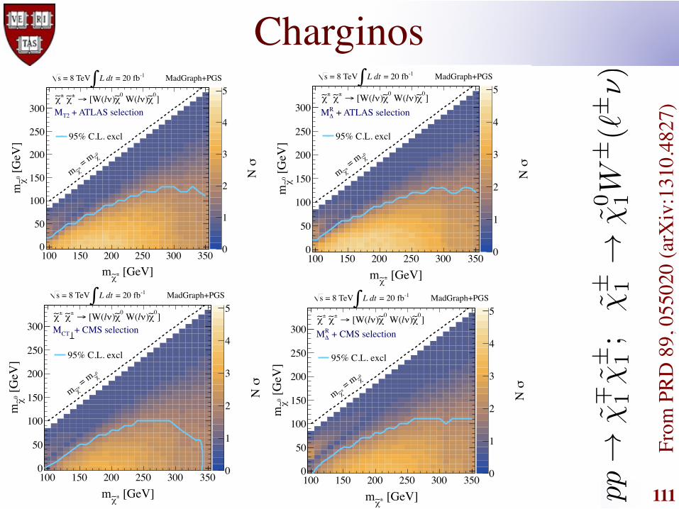
Charginos
111
[GeV]±χ∼m
100 150 200 250 300 350
[GeV
]0 χ∼
m
0
50
100
150
200
250
300
σN
0
1
2
3
4
5]0
χ∼)νl W(0χ∼)νl [W(→ ±χ∼ ±χ∼
+ ATLAS selection∆RM
-1 = 20 fbL dt ∫ = 8 TeV s MadGraph+PGS
95% C.L. excl
0χ∼
= m±χ∼m
[GeV]±χ∼m
100 150 200 250 300 350
[GeV
]0 χ∼
m
0
50
100
150
200
250
300
σN
0
1
2
3
4
5]0
χ∼)νl W(0χ∼)νl [W(→ ±χ∼ ±χ∼
+ ATLAS selectionT2M
-1 = 20 fbL dt ∫ = 8 TeV s MadGraph+PGS
95% C.L. excl
0χ∼
= m±χ∼m
[GeV]±χ∼m
100 150 200 250 300 350
[GeV
]0 χ∼
m
0
50
100
150
200
250
300
σN
0
1
2
3
4
5]0
χ∼)νl W(0χ∼)νl [W(→ ±χ∼ ±χ∼
+ CMS selectionCTM
-1 = 20 fbL dt ∫ = 8 TeV s MadGraph+PGS
95% C.L. excl
0χ∼
= m±χ∼m
[GeV]±χ∼m
100 150 200 250 300 350
[GeV
]0 χ∼
m
0
50
100
150
200
250
300
σN
0
1
2
3
4
5]0
χ∼)νl W(0χ∼)νl [W(→ ±χ∼ ±χ∼
+ CMS selection∆RM
-1 = 20 fbL dt ∫ = 8 TeV s MadGraph+PGS
95% C.L. excl
0χ∼
= m±χ∼m
From
PRD
89,
055
020
(arX
iv:1
310.
4827
)

Christopher Rogan - University of Chicago HEP - March 9, 2015
Super-Razor Basis Selection
112
[GeV]±χ∼m
100 150 200 250 300 350
[GeV
]0 χ∼
m
0
50
100
150
200
250
300
σN
0
1
2
3
4
5]0
χ∼)νl W(0χ∼)νl [W(→ ±χ∼ ±χ∼
+ Razor selectionRθ cos × β
Rφ∆ × ∆
RM
-1 = 20 fbL dt ∫ = 8 TeV s MadGraph+PGS
95% C.L. excl0χ∼
= m±χ∼m
[GeV]Ll~m
100 150 200 250 300 350 400 450
[GeV
]0 χ∼
m0
50
100
150
200
250
300
350
400
σN
0
1
2
3
4
50χ∼ l 0
χ∼ l → Ll~ Ll
~
+ Razor selectionRθ cos × β
Rφ∆ × ∆
RM
-1 = 20 fbL dt ∫ = 8 TeV s MadGraph+PGS
95% C.L. excl0χ∼
= mLl~m
From PRD 89, 055020 (arXiv:1310.4827 [hep-ph])

Christopher Rogan - University of Chicago HEP - March 9, 2015 113
Comparisons
[GeV]±χ∼ m150 200 250 300 350
σN
0
1
2
3
4
5 + ATLAS selectionT2M
+ ATLAS selection∆RM
Rθ cos × βRφ∆ × ∆RM
]0χ∼)νl[W(× 2→ ±χ∼ ±χ∼
= 100 GeV0χ∼ m
-1 = 20 fbL dt ∫ = 8 TeV s MadGraph+PGS
95% C.L.
[GeV]±χ∼ m150 200 250 300 350
σN
0
1
2
3
4
5 + CMS selectionCTM
+ CMS selection∆RM
Rθ cos × βRφ∆ × ∆RM
]0χ∼)νl[W(× 2→ ±χ∼ ±χ∼
= 100 GeV0χ∼ m
-1 = 20 fbL dt ∫ = 8 TeV s MadGraph+PGS
95% C.L.
[GeV]0χ∼ m
0 50 100 150 200
σN
0
1
2
3
4
5
6
7 + CMS selectionCTM
+ CMS selection∆RM
Rθ cos × βRφ∆ × ∆RM
]0χ∼)νl[W(× 2→ ±χ∼ ±χ∼
= 250 GeV±χ∼ m
-1 = 20 fbL dt ∫ = 8 TeV s MadGraph+PGS
95% C.L.
[GeV]0χ∼ m
0 50 100 150 200
σN
0
1
2
3
4
5
6
7 + ATLAS selectionT2M
+ ATLAS selection∆RM
Rθ cos × βRφ∆ × ∆RM
]0χ∼)νl[W(× 2→ ±χ∼ ±χ∼
= 250 GeV±χ∼ m
-1 = 20 fbL dt ∫ = 8 TeV s MadGraph+PGS
95% C.L.
From
PRD
89,
055
020
(arX
iv:1
310.
4827
)