kinetic modelling of lactic acid production from...
TRANSCRIPT
Kinetic Modelling of Lactic Acid Production from Whey
By
Duygu ALTIOK
A Dissertation Submitted to the Graduate School in Partial Fulfillment of the
Requirements for the Degree of
MASTER OF SCIENCE
Department : Food Engineering Major : Food Engineering
Izmir Institute of Technology Izmir, Turkey
July, 2004
We approve the thesis of Duygu ALTIOK
Date of Signature
...................................................... 30.07.2004 Assist. Prof. Figen TOKATLI Supervisor Department of Food Engineering ...................................................... 30.07.2004 Prof. Dr. �ebnem HARSA Co-Supervisor Department of Food Engineering ...................................................... 30.07.2004 Assist. Prof. Canan TARI Department of Food Engineering ...................................................... 30.07.2004 Assist. Prof. Sevcan ÜNLÜTÜRK Department of Food Engineering ...................................................... 30.07.2004 Assist. Prof. O�uz BAYRAKTAR Department of Chemical Engineering ...................................................... 30.07.2004 Prof. Dr. �ebnem HARSA Head of Food Engineering Department

ACKNOWLEDGMENTS
I would like to express my sincere gratitude to my supervisor Assist. Prof. Figen
Tokatlı and co-supervisor Prof. Dr. �ebnem Harsa for their guidance, supervision,
encouragement, and support throughout my research.
I would also express special thanks to my lovely husband, Research Assistant
Evren Altıok, for his endless support, encouragement and understanding.
I would like to thank to Zelal Polat for helps in laboratory works.

ABSTRACT
Lactic acid is a natural organic acid, which is used in pharmaceuticals, chemical,
textile and food industries. Since only L(+) lactic acid is found in normal human
metabolism, the microbial production of L(+) lactic acid has great interest in recent
years. Use of whey lactose to produce lactic acid by fermentation process is favourable
due to the low cost of whey and its high organic matter content. Whey is suitable
medium for some fermentations. However, its high lactose content makes it a potential
environmental pollutant. The disposal problem of this pollutant could be overcome by
utilization of whey lactose in the lactic acid production.
The aim of this study was to develop a kinetic model for lactic acid production
from whey by Lactobacillus casei, which is a homofermentative lactic acid bacteria and
capable of producing L(+) lactic acid. Within this context, several batch fermentation
experiments in fermenter were performed at 37 oC and pH 5.5. Seed culture that was
produced in shake flask fermentations was used as the inoculum for the fermenter.
Before the fermentation experiments, some of the proteins in whey were
denatured by heat treatment and separated by centrifugation. This treatment decreased
the protein amount from 11.15 % to 5.2 % in whey powder. The lactic acid production
was associated with the biomass growth up to a certain time, but then a non-growth
associated lactic acid production was observed in most of the fermentations except for
the 9.0 g l-1 initial substrate fermentation run, where all the substrate was utilized when
the stationary phase was attained. The maximum theoretical productivity was obtained
as 2.4 g lactic acid l-1 h-1 in the fermentation with S0 equals to 35.5 g l-1. The kinetic
parameters were obtained from different fermentation runs. µmax and KS were found as
0.265 h-1 and 0.72 g l-1, respectively. The average product yield coefficient, YPS, was
determined as 0.682 g lactic acid (g lactose)-1.
The modified form of logistic equation with product inhibition term for biomass
growth, Luedeking and Piret equation for product formation and substrate utilization
considering the consumption of substrate for product formation and maintenance,
described most of the fermentation experiments in this study with high accuracy (SSE
range was 0.0804-0.1531). The toxic powers in these inhibition terms, h and f, made
the model applicable for the fermentation experiments with low and high initial
substrate concentrations. In case of high initial substrate concentration fermentation

v
(S0= 95.7 g l-1), the same model explains only the exponential phase of biomass and its
product formation eventhough the substrate consumption is predicted very well.
ÖZ
Do�al bir organik asit olan laktik asit farmasütik, kimya, tekstil ve gıda
endüstrilerinde önemli bir yere sahiptir. �nsan metabolizmasında sadece L(+) laktik asit
izomeri bulundu�undan, bu izomerin mikrobiyal yoldan eldesi son zamanlarda çok ilgi
çekmektedir. Laktik asitin fermentasyonla eldesinde kullanılan peynir suyundaki laktoz,
peynir suyunun ucuz olması ve organic madde içeri�inin yüksek olmasından dolayı
tercih edilir. Peynir suyu bazı fermentasyonlar için uygun bir substrattır ancak yüksek
laktoz içerdi�inden dolayı potansiyel bir çevre kirleticisidir. Peynir suyundaki laktozun
fermentasyon sırasında tüketimi çok de�erli bir ürün olan laktik asitin eldesinin yanısıra
bu kirletici maddenin yok edilmesini de sa�lar.
Bu çalı�manın amacı, homofermentatif laktik asit bakterisi olan ve L(+)
izomerini üretebilen Lactobacillus casei ile peynir suyundan laktik asit eldesinin de�i�ik
laktoz konsantrasyonlarında kinetik modellemesi ve geli�tirilmesidir. Bu çerçevede, 37 oC ve pH 5.5’ de kesikli fermentasyonlar yapılmı�tır. Çalkalamalı inkübatörde elde
edilen kültür, fermentör için inokulum olarak kullanılmı�tır.
Fermentasyon çalı�malarından önce peynir suyundaki proteinlerin bir kısmı ısıl
i�lemle denetüre edilmi� ve santrifüj ile ayrılmı�tır. Bu i�lemler peynir suyu tozundaki
protein miktarını 11.15 %’den 5.2 %’ye dü�ürmü�tür. Laktik asit belli bir saate kadar
biomas art�ına ba�lı olarak üretilmi� daha sonra büyümeden ba�ımsız olarak
üretilmi�tir. Ancak 9.0 g l-1 ba�langıç substrat konsantrasyonuyla yapılan
fermentasyonda dura�an faza ula�madan önce substratın tamamı tüketilmi�tir.
Maksimum teorik üretkenlik 35.5 g l-1 ba�langıç substratlı fermentasyonda 2.4 g laktik
asit l-1 h-1 olarak elde edilmi�tir. Kinetik parametreler de�i�ik fermentasyon
çalı�malarından elde edilmi�tir. µmax ve KS sırasıyla 0.265 h-1 ve 0.72 g l-1 olarak
bulunmu�tur. Ürün verim katsayısı ortalama de�eri 0.682 g laktik asit (g laktoz)-1 olarak
saptanmı�tır. Mikrobiyal büyüme için lojistik denklemin ürün inhibisyon terimi ile
modifiye edilmi� formu, ürün olu�umu için Luedeking ve Piret’in belirtti�i denklem ve
substrat tüketimini ürün olu�umu ve temel metabolik faaliyetleri göz önünde
bulundurarak açıklayan denklem bu çalı�madaki fermentasyonların ço�unu büyük
do�rulukla açıklamı�tır. �nhibisyon terimlerindeki toksik kuvvetler, inhibisyon etkisini
ba�langıç substrat konsantrasyonu dü�ük oldu�unda önemsiz, yüksek oldu�u
durumlarda ise önemli kılarak modelin de�i�ik fermentasyonlara uygulanabilirli�ini
arttırmı�tır. Yüksek ba�langıç substrat konsantrasyonlu fermentasyonda (S0= 95.7 g l-1),

vii
model substrat tüketimini çok iyi açıklayabilmesine ra�men mikrobiyal büyümeyi ve
ürün olu�umunu sadece logaritmik faz için açıklayabilmi�tir.
TABLE OF CONTENTS
LIST OF FIGURES .......................................................................................................... x
LIST OF TABLES......................................................................................................... xiv
NOMENCLATURE ....................................................................................................... xv
Chapter 1. INTRODUCTION........................................................................................... 1
Chapter 2. LACTIC ACID................................................................................................ 3
2.1. History and Applications of Lactic Acid ....................................................... 3
2.2. Properties of Lactic Acid ............................................................................... 4
2.3. Microbial Production ..................................................................................... 5
2.3.1. Microorganisms and Raw Materials ............................................... 5
2.3.2. Fermentation and Recovery Processes ........................................... 9
Chapter 3. MODELLING............................................................................................... 11
3.1. Model Types ................................................................................................ 11
3.2. Microbial Growth Curve and Microbial Products ....................................... 13
3.3. Kinetic Models............................................................................................. 16
Chapter 4. MATERIALS AND METHODS.................................................................. 21
4.1. Materials ...................................................................................................... 21
4.2. Methods ....................................................................................................... 21
4.2.1. Culture Propagation ...................................................................... 21
4.2.2. Pretreatment of Whey ................................................................... 21
4.2.3. Lactic Acid Fermentations............................................................ 22
4.2.4. Analyses........................................................................................ 23
4.2.4.1. Lactose and Lactic Acid Analyses................................. 23
4.2.4.2. Determination of Biomass Concentration...................... 24
4.2.4.3. Determination of Protein Concentration of Whey......... 25
4.3. Kinetic Equations & Parameter Estimation ................................................. 25
4.3.1. Kinetic and Stoichiometric Parameters......................................... 26
ix
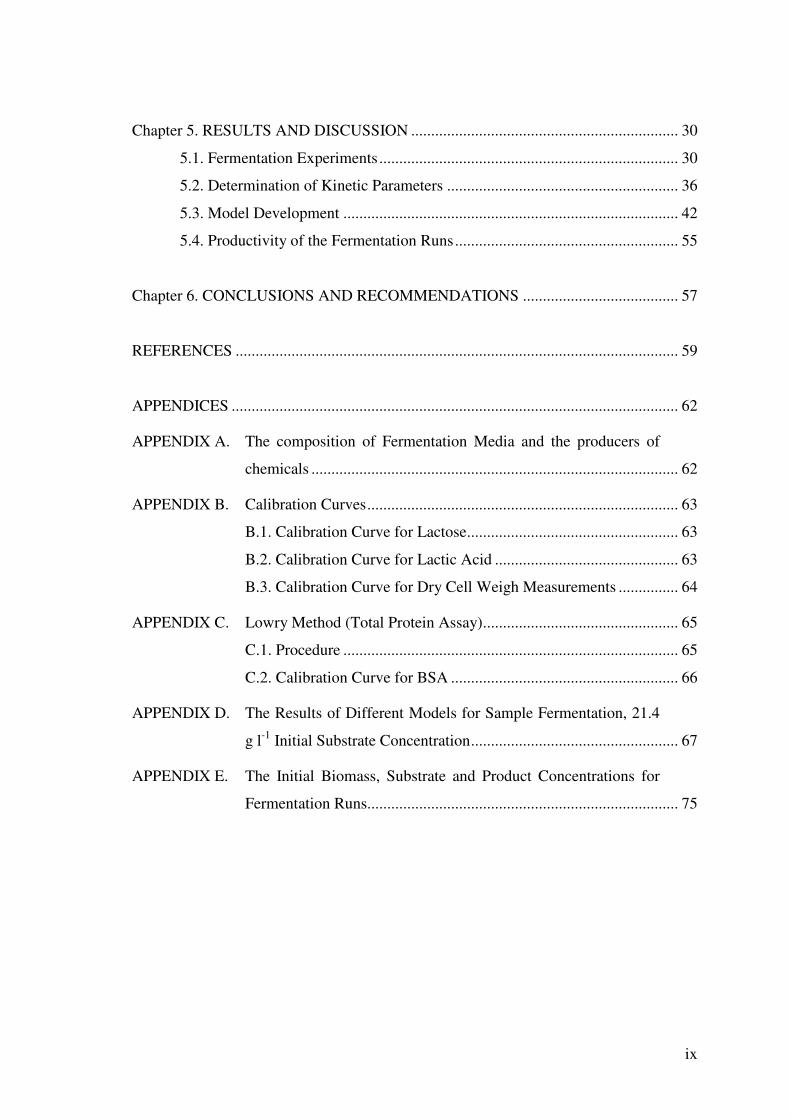
Chapter 5. RESULTS AND DISCUSSION ................................................................... 30
5.1. Fermentation Experiments........................................................................... 30
5.2. Determination of Kinetic Parameters .......................................................... 36
5.3. Model Development .................................................................................... 42
5.4. Productivity of the Fermentation Runs........................................................ 55
Chapter 6. CONCLUSIONS AND RECOMMENDATIONS ....................................... 57
REFERENCES ............................................................................................................... 59
APPENDICES ................................................................................................................ 62
APPENDIX A. The composition of Fermentation Media and the producers of
chemicals ............................................................................................ 62
APPENDIX B. Calibration Curves.............................................................................. 63
B.1. Calibration Curve for Lactose..................................................... 63
B.2. Calibration Curve for Lactic Acid .............................................. 63
B.3. Calibration Curve for Dry Cell Weigh Measurements ............... 64
APPENDIX C. Lowry Method (Total Protein Assay)................................................. 65
C.1. Procedure .................................................................................... 65
C.2. Calibration Curve for BSA ......................................................... 66
APPENDIX D. The Results of Different Models for Sample Fermentation, 21.4
g l-1 Initial Substrate Concentration.................................................... 67
APPENDIX E. The Initial Biomass, Substrate and Product Concentrations for
Fermentation Runs.............................................................................. 75

LIST OF FIGURES
Figure 2.1. Isomers of lactic acid .............................................................................. 4
Figure 2.2. L casei NRRL B-441 .............................................................................. 6
Figure 3.1. Different perspectives for cell population kinetic
representations ...................................................................................... 12
Figure 3.2. Microbial Growth Curve....................................................................... 14
Figure 3.3. Kinetic patterns of product formation in batch
fermentations: (a) growth-associated product formation,
(b) nongrowth-associated product formation, (c) mixed-
growth-associated product formation ................................................... 16
Figure 3.4. The relationship between growth rate and substrate
concentration......................................................................................... 17
Figure 3.5. Specific rate of product synthesis as a function of the
specific rate of bacterial growth during batch
fermentations ........................................................................................ 18
Figure 4.1. Monod kinetics ..................................................................................... 27
Figure 4.2. Double reciprocal (Lineweaver-Burk) plot........................................... 28
Figure 5.1. Experimental results of fermentation with 9.0 g l-1 initial
substrate concentration ......................................................................... 31
Figure 5.2. Experimental results of fermentation with 21.4 g l-1 initial
substrate concentration ......................................................................... 32
Figure 5.3. Experimental results of fermentation with 35.5 g l-1 initial
substrate concentration ......................................................................... 32
Figure 5.4. Experimental results of fermentation with 48.0 g l-1 initial
substrate concentration ......................................................................... 33
Figure 5.5. Experimental results of fermentation with 61.2 g l-1 initial
substrate concentration ......................................................................... 34
Figure 5.6. Experimental results of fermentation with 77.1 g l-1 initial
substrate concentration ......................................................................... 35
Figure 5.7. Experimental results of fermentation with 95.7 g l-1 initial
substrate concentration ......................................................................... 36
Figure 5.8. Relation between the product yield coefficient and initial
substrate concentration ......................................................................... 37
xi
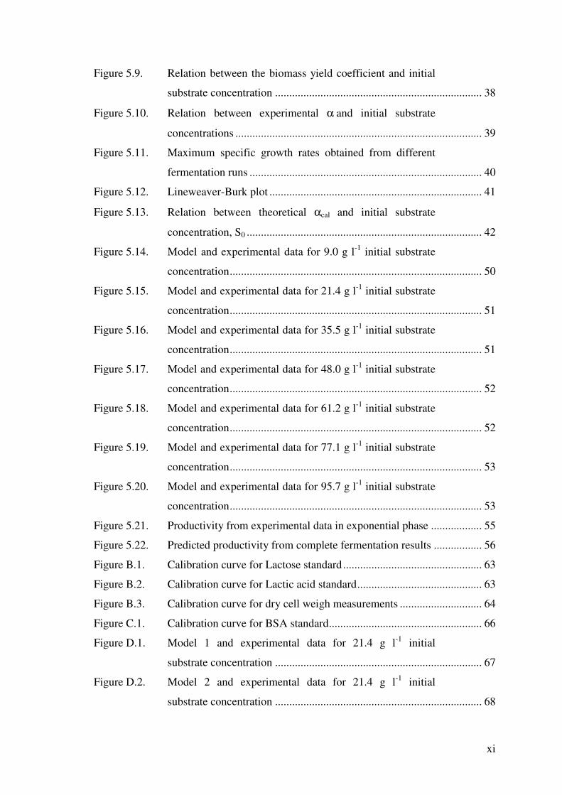
Figure 5.9. Relation between the biomass yield coefficient and initial
substrate concentration ......................................................................... 38
Figure 5.10. Relation between experimental α and initial substrate
concentrations ....................................................................................... 39
Figure 5.11. Maximum specific growth rates obtained from different
fermentation runs .................................................................................. 40
Figure 5.12. Lineweaver-Burk plot ........................................................................... 41
Figure 5.13. Relation between theoretical αcal and initial substrate
concentration, S0 ................................................................................... 42
Figure 5.14. Model and experimental data for 9.0 g l-1 initial substrate
concentration......................................................................................... 50
Figure 5.15. Model and experimental data for 21.4 g l-1 initial substrate
concentration......................................................................................... 51
Figure 5.16. Model and experimental data for 35.5 g l-1 initial substrate
concentration......................................................................................... 51
Figure 5.17. Model and experimental data for 48.0 g l-1 initial substrate
concentration......................................................................................... 52
Figure 5.18. Model and experimental data for 61.2 g l-1 initial substrate
concentration......................................................................................... 52
Figure 5.19. Model and experimental data for 77.1 g l-1 initial substrate
concentration......................................................................................... 53
Figure 5.20. Model and experimental data for 95.7 g l-1 initial substrate
concentration......................................................................................... 53
Figure 5.21. Productivity from experimental data in exponential phase .................. 55
Figure 5.22. Predicted productivity from complete fermentation results ................. 56
Figure B.1. Calibration curve for Lactose standard................................................. 63
Figure B.2. Calibration curve for Lactic acid standard............................................ 63
Figure B.3. Calibration curve for dry cell weigh measurements ............................. 64
Figure C.1. Calibration curve for BSA standard...................................................... 66
Figure D.1. Model 1 and experimental data for 21.4 g l-1 initial
substrate concentration ......................................................................... 67
Figure D.2. Model 2 and experimental data for 21.4 g l-1 initial
substrate concentration ......................................................................... 68

xii
Figure D.3. Model 3 and experimental data for 21.4 g l-1 initial
substrate concentration ......................................................................... 69
Figure D.4. Model 4 and experimental data for 21.4 g l-1 initial
substrate concentration ......................................................................... 70
Figure D.5. Model 5 and experimental data for 21.4 g l-1 initial
substrate concentration ......................................................................... 71
Figure D.6. Model 6 and experimental data for 21.4 g l-1 initial
substrate concentration ......................................................................... 72
Figure D.7. Model 7 and experimental data for 21.4 g l-1 initial
substrate concentration ......................................................................... 73
Figure D.8. Model 8 and experimental data for 21.4 g l-1 initial
substrate concentration ......................................................................... 74
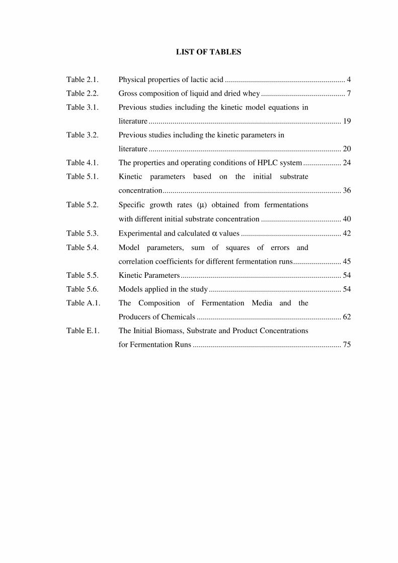
LIST OF TABLES
Table 2.1. Physical properties of lactic acid ............................................................ 4
Table 2.2. Gross composition of liquid and dried whey.......................................... 7
Table 3.1. Previous studies including the kinetic model equations in
literature ................................................................................................ 19
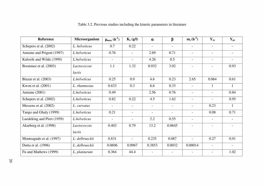
Table 3.2. Previous studies including the kinetic parameters in
literature ................................................................................................ 20
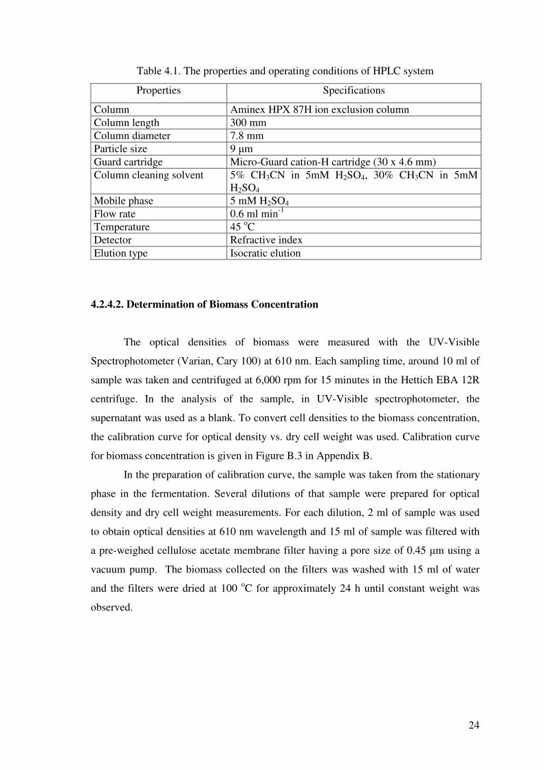
Table 4.1. The properties and operating conditions of HPLC system ................... 24
Table 5.1. Kinetic parameters based on the initial substrate
concentration......................................................................................... 36
Table 5.2. Specific growth rates (µ) obtained from fermentations
with different initial substrate concentration ........................................ 40
Table 5.3. Experimental and calculated α values .................................................. 42
Table 5.4. Model parameters, sum of squares of errors and
correlation coefficients for different fermentation runs........................ 45
Table 5.5. Kinetic Parameters ................................................................................ 54
Table 5.6. Models applied in the study .................................................................. 54
Table A.1. The Composition of Fermentation Media and the
Producers of Chemicals ........................................................................ 62
Table E.1. The Initial Biomass, Substrate and Product Concentrations
for Fermentation Runs .......................................................................... 75
2
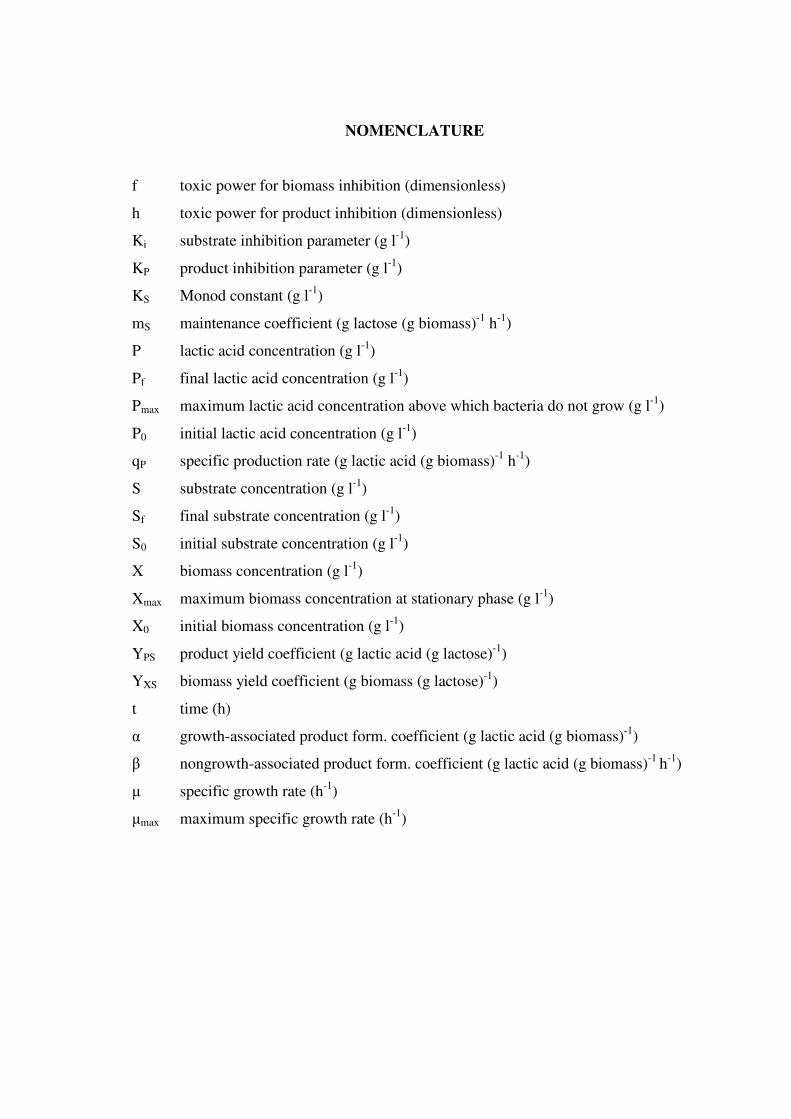
NOMENCLATURE
f toxic power for biomass inhibition (dimensionless)
h toxic power for product inhibition (dimensionless)
Ki substrate inhibition parameter (g l-1)
KP product inhibition parameter (g l-1)
KS Monod constant (g l-1)
mS maintenance coefficient (g lactose (g biomass)-1 h-1)
P lactic acid concentration (g l-1)
Pf final lactic acid concentration (g l-1)
Pmax maximum lactic acid concentration above which bacteria do not grow (g l-1)
P0 initial lactic acid concentration (g l-1)
qP specific production rate (g lactic acid (g biomass)-1 h-1)
S substrate concentration (g l-1)
Sf final substrate concentration (g l-1)
S0 initial substrate concentration (g l-1)
X biomass concentration (g l-1)
Xmax maximum biomass concentration at stationary phase (g l-1)
X0 initial biomass concentration (g l-1)
YPS product yield coefficient (g lactic acid (g lactose)-1)
YXS biomass yield coefficient (g biomass (g lactose)-1)
t time (h)
� growth-associated product form. coefficient (g lactic acid (g biomass)-1)
� nongrowth-associated product form. coefficient (g lactic acid (g biomass)-1 h-1)
� specific growth rate (h-1)
�max maximum specific growth rate (h-1)

CHAPTER 1
INTRODUCTION
Lactic acid is a natural organic acid, which is an industrially important product.
It is used in pharmaceuticals, cosmetics, and chemical, textile and food industries. It
exists in two optically active forms, D(-) and L(+) lactic acid. Lactic acid can be
produced industrially by chemical synthesis and microbial fermentation process. It is
synthetically produced by the hydrolyses of lactonitrile. Chemical synthesis yields only
the racemic (DL) lactic acid. However, L(+) lactic acid is the preferred isomer.
Therefore, there is a continued interest in the microbial production of L(+) lactic acid in
recent years.
Lactose in some organic compounds can be converted to lactic acid by some
lactic acid bacteria. Whey is one of these organic compounds used in lactic acid
production, which is a clean, abundant food-grade material and a potential
environmental pollutant due to its high lactose content. One of the promising ways to
use lactose in whey is to use it as a low cost carbon source for the production of organic
acids by fermentation. Disposal of whey and doing it profitably continues to be a
problem which confronts the entire cheese industry. Pollution of the environment and
loss of valuable nutrients are considerations, which militate against traditional disposal
methods. Use of a fermentation process to upgrade the nutritional quality of whey or to
produce a product with improved palatability was taught as an alternative procedure. In
short, the utilization of lactose in whey by fermentation overcomes the disposal problem
of this pollutant while it produces value-added end products such as lactic acid.
Lactobacillus casei is found in many food products as well as in the human body
and other natural environments. So, it is generally regarded as safe (GRAS) organism. It
is capable of fermenting whey lactose to L(+) lactic acid only, which is the lactic acid
isomer found in normal human metabolism and has wide applications in industry.
Therefore, highly pure preparations of L-lactic acid are in demand as a raw material for
the production of biodegradable lactide polymers used in the biomaterial manufacturing.
Lactobacillus casei produces about 97.5 % of the lactic acid in the L(+) form (Vaccari
et al. 1993). Most of the other lactic acid bacteria produce DL and D lactic acids.
2
Lactic acid can be obtained from whey by batch fermentation. In batch
fermentation system, the microorganism is inoculated after the sterilization of reactor
and fermentation media. During fermentation, the culture goes through different growth
phases. Different products are produced during these phases. To understand the
behaviour of the system, modelling is required. Models are used to define the
biological, chemical and physical basis of the process. A kinetic model is a set of
relationships between biomass growth, substrate utilization and product formation.
Kinetic models predict how fast the microorganisms can grow and use substrates or
make products. In practice, kinetic data are collected with respect to time in small-scale
reactors and then used to scale-up the process along the mass transfer data.
The aim of this study is to develop the kinetic model to explain the lactic acid
production from whey by Lactobacillus casei. With in this context, batch fermentation
experiments with seven different initial substrate concentrations in a range of [9.0 g
lactose l-1 – 95.7 g lactose l-1] were performed to determine kinetic parameters such as
maximum growth rate (µmax), Monod constant (Ks), yield coefficients (YXS and YPS).

CHAPTER 2
LACTIC ACID
2.1. History and Applications of Lactic Acid
Lactic acid, 2-hydroxypropionic acid (CH3CHOHCOOH), was isolated and
identified by Scheele in 1780. Charles E. Avery set up the first commercial lactic acid
fermentation plant in Littleton, MA, in 1881. Worldwide consumption of lactic acid is
about 45,000 ton (year)-1, of which roughly 40 % belongs to the United States. Lactic
acid is used in many food and nonfood applications. In 1989, 7,600 ton were used for
the manufacture of emulsifiers, 4,400 ton in food additives, 1,700 ton for
pharmaceutical and cosmetics applications, and the balance for industrial and
miscellaneous uses (Vick Roy 1985). It is a natural organic acid and industrially
important product with a large market due to its attractive properties. For example, the
acid and salts are preferred to other acids in the food industry because they do not
dominate other flavors and also act as preservatives where it is used as an acidulant and
a flavour enhancer in many kinds of foods or beverages, such as beer, jellies, cheese,
and dried egg whites. The major use of synthetic and heat-stable lactic acid is in the
manufacture of sodium and calcium stearoyl lactylate and other lactylated emulsifiers.
Stearoyl lactylate is used in the baking industry as a dough conditioner. Furthermore,
the possibility of directly converting lactic acid to acrylic acid has also turned lactic acid
into an important raw material for the chemical industry (Hui and Khachatourians
1995). Recently, new applications for lactic acid such as biodegredable plastics
(polylactide polymers, polyhydroxybutryate) have accelerated research on its
production as a bulk raw material. Lactic acid is also used in pharmaceuticals,
cosmetics, and textile industries (Roukas and Kotzekidou 1998).
Lactic acid from cheese whey is produced commercially in Slovakia, Italy, and
the United States, whereas synthetic production from acetaldehyde or lactonitrile is
cheaper, the low cost of whey makes a large-scale production facility competitive.
Lactic acid bacteria such as Lactococcus lactis, Lactobacillus delbrueckii subsp.
bulgaricus, Lactobacillus acidophilus, Lactobacillus helveticus, Lactobacillus casei,

4
and mixed cultures of these organisms have been successfully used to convert lactose to
lactic acid (Henning 1998).
2.2. Properties of Lactic Acid
Lactic acid is the simplest 2-hydroxyacid having a chiral centre, and exists as
two enantiomers, L(+) lactic acid and D(-) lactic acid. L(+) lactic acid is the enantiomer
involved in normal human metabolism (Hui and Khachatourians 1995). Figure 2.1
shows these isomers of lactic acid. Some of the physical properties of lactic acid are
given in Table 2.1.
Table 2.1. Physical properties of lactic acid (Vick Roy 1985)
Molecular weight 90.08 Melting Point D(-) or L(+) 52.8-54 oC Boiling Point DL 82 oC at 0.5 mmHg
122 oC at 14 mmHg Dissociation Constant (Ka at 25 oC) 1.37 x 10⁻⁴ Heat of Combustion (�Hc) 1361 kJ mol-1 Specific Heat (Cp at 20 oC) 190 J mol-1 oC-1
CO2H CO2H
HO C H H C OH
CH3 CH3
L(+) lactic acid D(-) lactic acid
Figure 2.1. Isomers of lactic acid. (Vick Roy 1985)
Optically active, high-purity lactic acid can form colourless monoclinic crystals.
Lactic acid may form a cyclic dimer (lactide) or form linear polymers with the general
formula H[OCH(CH3)CO]nOH. It may participate both as an organic acid and an
organic alcohol in several types of chemical reactions. Lactic acid is soluble in all
proportions with water and exhibits a low volatility. In solutions with roughly 20 % or

5
more lactic acid, self-esterification occurs because of the hydroxyl and carboxyl
functional groups (Vick Roy 1985).
2.3. Microbial Production
2.3.1. Microorganisms and Raw Materials
Microorganisms:
Lactobacilli are large group of rod-shaped bacteria, which can vary form long
and slender, sometimes curved, rods to short, often coryneform, coccobacilli. Lactic
acid bacteria and some fungi of the species Rhizopus produce lactic acid. Lactic acid
bacteria are gram-positive, non-sporing and usually nonmotile and are categorized as
facultative anaerobes, thus making the strict exclusion of air is unnecessary. Lactic acid
bacteria have limited biosynthetic capabilities, so that they require many vitamins
(especially B vitamins) amino acids, purines, and pyrimidines (Prescott 1996). They are
classified into 3 groups based on their metabolism of sugars. Group 1; species are
obligate homofermenters of hexoses to lactate and do not ferment pentoses. Group2;
species are facultative heterofermenters of hexoses which means that they ferment
hexoses by glycolysis to lactate or, under glucose limitation, to lactate, acetate, ethanol,
and formate. Also, they ferment pentoses to lactate and acetate by the phosphoketolase
pathway. Group 3 species are obligate heterofermenters of sugars.
Lactobacillus casei, is member of Group 2. These organisms ferment sugars
homofermentatively to L(+) lactic acid and do not produce NH3 from arginine. The
homofermentative lactic acid bacteria produce only lactic acid. On the other hand, the
heterofermentative lactic acid bacteria produce not only lactic acid, but also acetic acid,
carbon dioxide, ethanol and glycerol so it is undesirable because of by-product
formation. (Vick Roy 1985).
This species, like L. acidophilus, is a gram-positive, catalase-negative, rod-
shaped bacterium, which is facultative with regard to oxygen requirements. It is a
normal inhabitant of the small intestine and is resistant to bile. Although its optimum
growth temperature is nearly 37 oC, unlike L. acidophilus, it will grow at 15 oC (Cogan
and Accolas 1996). Lactobacilli are the most acid tolerant of the lactic acid bacteria,
preferring to initiate growth at acidic pH (5.5-6.2) (Frank and Hassan 1998).
6
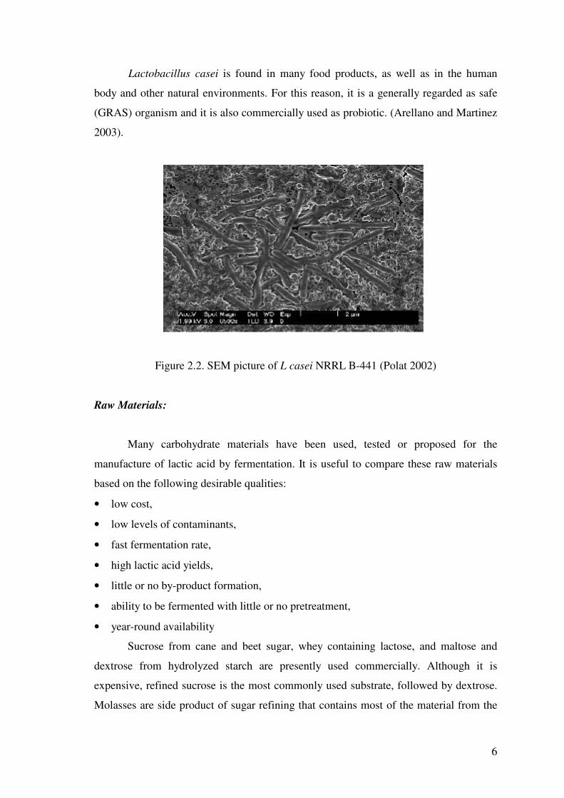
Lactobacillus casei is found in many food products, as well as in the human
body and other natural environments. For this reason, it is a generally regarded as safe
(GRAS) organism and it is also commercially used as probiotic. (Arellano and Martinez
2003).
Figure 2.2. SEM picture of L casei NRRL B-441 (Polat 2002)
Raw Materials:
Many carbohydrate materials have been used, tested or proposed for the
manufacture of lactic acid by fermentation. It is useful to compare these raw materials
based on the following desirable qualities:
• low cost,
• low levels of contaminants,
• fast fermentation rate,
• high lactic acid yields,
• little or no by-product formation,
• ability to be fermented with little or no pretreatment,
• year-round availability
Sucrose from cane and beet sugar, whey containing lactose, and maltose and
dextrose from hydrolyzed starch are presently used commercially. Although it is
expensive, refined sucrose is the most commonly used substrate, followed by dextrose.
Molasses are side product of sugar refining that contains most of the material from the

7
sugar beet or sugar cane, which is not sugar, molasses is one of the cheapest substrate
available. Malt extract is made from malted barley by soaking it in water (Bains 1993).
Whey is a by-product of the cheese-making process.
Among many carbohydrate materials used for the production of lactic acid,
cheese whey lactose deserves special consideration. Cheese whey is a clean,
wholesome, abundant food-grade material and a potential environmental pollutant. It is
the product separated from milk during cheesemaking and consists of water, lactose,
proteins, vitamins, and mineral salts (Roukas and Kotzekidou 1998).
The gross composition of dried and liquid cheese whey is given in Table 2.2.
Table 2.2. Gross composition of liquid and dried whey (Henning 1998)
Component Liquid whey Dried whey
Total solids, % 6.35 96.5
Protein, % 0.8 13.1
Lactose, % 4.85 75.0
Fat, % 0.5 0.8
Minerals and Vitamins, % 0.6 1.2
Lactic acid, % 0.05 0.2
Ash, % 0.5 7.3
About 57 billion pounds of liquid whey are produced each year in the U.S.
There is an interest in the economic utilization of the large quantities of cheese whey
produced by the dairy industry, because of the environmental problem caused by its
high organic matter content, essentially due to its lactose content. Disposal of whey and
doing it profitably continues to be a problem which confronts the entire cheese industry
(Amrane 2001).
There is continued interest in utilizing lactose from cheese whey for the
production of value-added end products. Several researchers have utilized anaerobes or
facultative anaerobes to ferment lactose to single cell protein, ethanol, biogas, lactic
acid and acetate (Tango and Ghaly 1999).
One of the promising ways to use lactose in whey is to use it as a low cost
carbon source for the production of organic acids by fermentation. This is not only
because of the fact that organic acids are valuable raw materials for the production of

8
high value end products, but also because of the fact that organic acids such as lactic
acid are easily metabolized compared to lactose in many fermentation processes (Fu and
Mathews 1999).
Whey is suitable as a medium for only some fermentations. This is true because
of its peculiar composition. The composition of whey is variable because cheese making
procedures and milk composition are not constant. Data on composition of whey
indicates that lactose is the only fermentable carbohydrate in whey. This means that the
use of whey is limited to those fermentations that employ microorganisms, which can
utilize lactose (Marth 1973).
Nitrogenous sources such as malt sprouts, malt extract, corn-steep liquor, barley,
yeast extract or undenaturated milk must supplement most carbohydrate sources to give
fast and heavy growth. Some growth promoting substances in these nitrogen sources are
sensitive to heat. In commercial practice, minimal amounts of substances are used in
order to simplify the recovery process.
Additional minerals are occasionally required when the carbohydrate and
nitrogenous sources lack sufficient quantities. Calcium carbonate and calcium
hydroxide are typically used to neutralize the acid that is formed (Vick Roy 1985).
Numerous methods are available to separate or fractionate whey proteins. An
important process for separating proteins from whey is ultrafiltration. Other protein
separation processes include heat-acid precipitation, coprecipitation, chemical
precipitation, ion-exchange and gel filtration. Maximum protein recovery is obtained by
denaturing whey proteins at pH in the range of 6-7 and temperatures greater than 90 oC
for 10-30 min, followed by precipitation at pH 4.5-5.5. Heating at neutral pH induces
primary aggregation through S-S bridges, which must proceed isoelectric precipitation
for maximum protein recovery. The theoretical maximum recovery of crude protein
from whey is 55-65 % because the heat stable proteose-peptone fraction constitutes 35-
45 % of whey nitrogen. Commercially feasible processes should recover at least 50 %
of the crude protein. Recovery of heat-precipitated whey proteins is normally best
accomplished by a centrifuge or decanter. For small operations, recovery of heat-
precipitation proteins from very sweet whey by filtration might be feasible (Irvine and
Hill 1985).
9
2.3.2. Fermentation and Recovery Processes
Fermentation Process:
Fermentation is the process where the microorganism metabolizes a substrate
under aerobic or anaerobic conditions.
The ideal fermentation would serve to;
• upgrade the nutritional properties of substrate
• improve its flavour and appearance so that a palatable product would result
• utilize all substrate without producing wastes that need to be treated
• produce a product which could be sold for more money than the cost of raw
materials (Marth 1973).
In batch fermentation system, the reactor is filled with a sterile nutrient substrate
and inoculated with microorganism. The culture is allowed to grow until no more of the
product is produced after which the reactor is ‘harvested’ and cleaned out for another
run. In batch culture, the culture environment changes continually. The culture goes
through lag phase, exponential phase, stationary phase, and death phase. Depending on
what the product is, the ‘useful’ part of the growth cycle can be any one of these four
stages, although it is usually the exponential or stationary phase (Bains 1993).
On the other hand, in continuous culture, fresh nutrient medium is continually
supplied to a well-stirred culture and products and cells are simultaneously withdrawn.
After a certain time, the system usually reaches a steady-state where cell, product, and
substrate concentration remain constant.
In fed-batch culture, nutrients are continuously or semicontinuously fed, while
effluent is removed discontinuously. Fed-batch culture is usually used to overcome
substrate inhibition or catabolite repression (Shuler and Kargi 2002).
Recovery Process:
Lactic acid is sold in three major grades: technical, food, and pharmaceutical.
The recovery of lactic acid or lactate salts from the fermentation broth covers the large
part of the total manufacture cost. Synthetically made lactic acid may be purified with
10
less effort and thus in the past has been preferred for uses where heat stability was
needed.
The first step in all recovery processes is to raise the fermentation liquor’s
temperature to 80-100 oC and increase the pH to 10 or 11. This procedure kills the
organisms, coagulates the proteins, solubilizes the calcium lactate, and degrades some
of the residual sugars. The liquid is the decanted or filtered. For some purposes,
acidification of this liquor yields a useable product; however, for most applications
further processing by one of the following methods is required. It should also be noted
that use of cheap but impure raw materials must be weighed against higher purification
costs. Filtration, carbon treatment and evaporation, calcium lactate crystallization,
liquid-liquid extraction, distillation of lactate esters are the basic recovery processes.
Lactic acid may also be recovered by the adsorption of lactic acid on solid adsorbents or
by the adsorption of lactate on ion-exchange resins (Vick Roy 1985).
11
CHAPTER 3
MODELLING
Modelling is an essential step in the development of the process under
consideration by predicting the behaviour of the system. A model is a set of
relationships between the variables of interest in the system being studied. Models are
mainly used for defining the biological, chemical, or physical basis of the process,
planning the experimental conditions and evaluating the experimental results (Sinclair
and Kristiansen 1987). The purpose of fermentation modelling is to design large-scale
fermentation processes using data obtained from small-scale fermentations (McNeil and
Harvey 1990).
3.1. Model Types
Several different models are used in fermentation engineering:
• Kinetic models predict how fast the microorganisms can grow and use substrates or
make products.
• Stoichiometric models predict how much substrate is needed or product is produced
given a known amount of biomass or vice versa.
• Transport models predict how fast for example oxygen can be transported to the
cells or how fast heat can be removed.
These different models can be put together into a process model, in order to
predict the combined effects of the biology and the physics in a fermenter. The
overriding factor that propels biotechnology is profit. The maximization of profits is
closely linked to optimising product formation by cellular catalysts; i.e. producing the
maximum amount of product in the shortest time at the lowest cost.
The large-scale cultivation of cells is central to the production of a large
proportion of commercially important biological products. Thus, cell culture system
must be described quantitatively. In other words, the kinetic of the process must be
known. By determining the kinetics of the system, it is possible to predict yields and
reaction times and thus permit the correct sizing of a bioreactor. In practice, kinetic data
is obtained in small-scale reactors and then used with mass transfer data to scale-up the
12
process (Bailey and Ollis 1986). A kinetic model can be very useful for the design of
both continuous and batch production systems.
In batch or fed batch fermentation processes, there is no steady state. The control
of a fermentation process is based on the measurement of physical, chemical or
biochemical properties of the fermentation broth and the manipulation of physical and
chemical environmental parameters (Carrillo-Ureta et al. 2001).
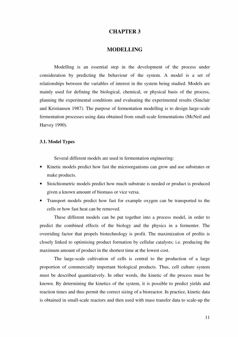
The cellular phase of the system was first represented by Arnold Fredrickson
and Henry Tsuchiya as in Figure 3.1. They classified approaches to microbial systems
according to the number of components used in the cellular representation and the
homogeneity of cell culture.
Unstructured Structured
Single component, heterogeneous
individual cells
Actual case
Multicomponent description of
cell-to-cell heterogeneity
Segregated
Cell population treated as one
component solute
Most idealized case
Multicomponent average cell
description
Unsegregated
Figure 3.1. Different perspectives for cell population kinetic representations (Bailey and
Ollis 1986)
The complete description of the growth kinetics of a culture would involve
recognition of the structured nature of each cell and the segregation of the culture into
individual units (cells) that may differ from each other. A chemically structured model
divides the cell mass into components. If the ratio of these components can change in
response to disturbances in the extracellular environment, then the model is behaving
analogously to a cell changing its composition in response to environmental changes
(Shuler and Kargi 2002). However, what can be termed an unstructured mechanism of
cell operation is sufficient for many technological purposes. In an unstructured

13
mechanism of cellular operation, the microorganism is regarded as a single reacting
species, possibly with a fixed chemical composition. Its limitations are improper use of
the processes, which occur within the cell, or ability to analyse cells for particular
constituents (Sinclair and Kristiansen 1987). Models may be structured and segregated,
structured and unsegregated, unstructured and segregated, unstructured and
unsegregated. Models containing both structure and segregation are the most realistic,
but they are also computationally complex. The degree of realism and complexity
required in a model depends on what is being described; the researcher should always
choose the simplest model that can adequately describe the system. An unstructured
model assumes fixed cell composition, which is equivalent to assuming balanced
growth (Shuler and Kargi 2002). In this study, the unstructured and unsegregated model
was developed.
3.2. Microbial Growth Curve and Microbial Products
Growth is the most essential response of microorganisms to their
physiochemical environment. It is a result of both replication and change in cell size.
Microorganisms can grow under different physical and chemical conditions.
They require substrates mainly:
• to synthesize new cell material
• to synthesize extracellular products
• to provide the energy necessary to maintain concentrations of materials within the
cells which differ from those in the environment and in synthetic reactions
Thus growth, substrate utilisation, maintenance and product formation are all
closely related (Sinclair and Kristiansen 1987). When a liquid nutrient medium is
inoculated with a seed culture, the organisms selectively take up dissolved nutrients
from the medium and convert them into biomass. In a typical batch process, the cell
number varies with time and the following phases occur: 1) lag phase, (2) logarithmic or
exponential growth phase, (3) deceleration phase, (4) stationary phase, and (5) death
phase.
Typical microbial growth curve can be seen in Figure 3.2.

14
Figure 3.2. Microbial Growth Curve
The lag phase, is an adaptation period of cells to a new environment, occurs
immediately after inoculation. During this adaptation period, new enzymes are
synthesised, and the synthesis of some other enzymes is suppressed. Cell mass may
increase, while cell number density remains constant. The lag period is affected from
the age and size of the inoculum culture and the nutrient medium. Usually, the lag
period increases with the age of the inoculum. To minimize the duration of the lag
phase, cells should be young and active, and the inoculum size should be large. The
nutrient medium may need to be optimised and certain growth factors can be included
in order to minimize the lag phase.
After this adaptation period, the cells adjust to their new environment, start to
multiply rapidly and consequently cell mass and cell number density increase
exponentially with time. Therefore, this period is named as exponential or logarithmic
growth phase.
The deceleration growth phase follows the exponential phase. In this phase,
growth decelerates due to either depletion of one or more essential nutrients or the
accumulation of toxic by-products of growth. For a typical bacterial culture, these
changes occur over a very short period of time.
The stationary phase starts at the end of the deceleration phase, when the net
growth rate is zero (no cell division) or when the growth rate is equal to the death rate.
Even though the net growth rate is zero during the stationary phase, cells are still
metabolically active and produce secondary metabolites. Primary metabolites are

15
growth-related products such as lactic acid, ethanol and secondary metabolites are
nongrowth-related products such as antibiotics. During the stationary phase, the cell
catabolizes cellular reserves for new building blocks and for energy-producing
monomers. This is called endogenous metabolism. The cell must always spend energy
to maintain an energised membrane and transport of nutrients and for essential
metabolic functions such as motility and repair of damage to cellular structures. This
energy expenditure is called maintenance energy.
The death phase follows the stationary phase. Often, death cells lyse, and a
cellular nutrients released into the medium are used by the living organisms during
stationary phase. At the end of the stationary phase, because of either nutrient depletion
or toxic product accumulation the death phase begins.
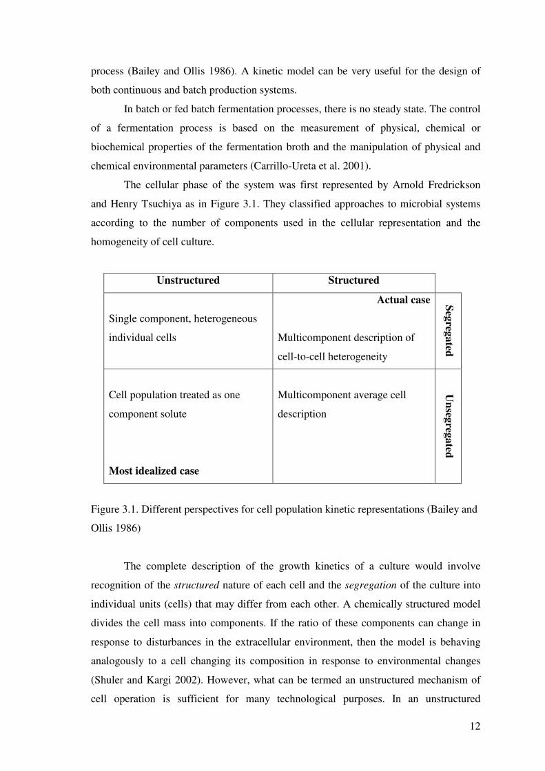
Microbial products can be classified in three major categories:
1. Growth-associated products are produced simultaneously with microbial growth.
The specific rate of product formation is proportional to the specific rate of growth. The
production of a constitutive enzyme is an example of a growth-associated product.
µPXp YdtdP
Xq == 1
(3.1)
2. Nongrowth-associated product formation takes place during the stationary phase
when the growth rate is zero. The specific rate of product formation is constant. Many
secondary metabolites, such as antibiotics (for example, penicillin), are nongrowth-
associated products.
== βPq constant (3.2)
3. Mixed-growth-associated product formation takes place during the slow growth and
stationary phases. In this case, the specific rate of product formation is given by the
following equation:
βαµ +=Pq (Luedeking-Piret equation) (3.3)
Lactic acid fermentation, xanthan gum, and some secondary metabolites from
cell culture are examples of mixed-growth-associated products (Shuler and Kargi 2002).
16
The kinetic pattern, of these types of product formation can be seen in Fig 3.3.
(a) (b) (c)
Figure 3.3. Kinetic patterns of product formation in batch fermentations: (a) growth-
associated product formation, (b) nongrowth-associated product formation, (c) mixed-
growth-associated product formation (Shuler and Kargi 2002).
3.3. Kinetic Models
The majority of kinetic models describing microbial growth use a formal
macroapproach to bioprocessing. They are empirical and based on either Monod’s
equation or on its numerous modifications which take into account the inhibition of
microbial growth by a high concentration of product and/or substrate.
The main objective of formulating a fermentation medium is to support good
growth and/or high rates of product formation. The amounts of all nutrients in the
medium are very critic. For example, excess concentration of a nutrient can inhibit cell
growth. Moreover, if the cells grow too extensively, their accumulated metabolic end
products will often disrupt the normal biochemical processes of the cells. Consequently,
it is common practice to limit total growth by limiting the amount of one nutrient in the
medium.
17
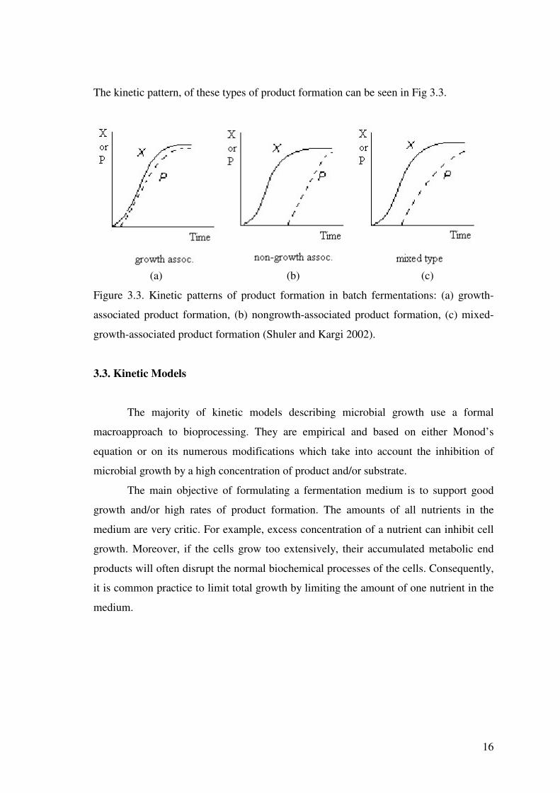
Figure 3.4. The relationship between growth rate and substrate concentration. (Bailey
and Ollis 1986)
By changing the concentration of one medium constituent and keeping the
others constant, the characteristics of growth rate can be obtained as in Figure 3.4.
Monod proposed a functional relationship between the specific growth rate �
and an essential compound’s concentration in 1942. This relationship is similar to the
Langmuir adsorption isotherm (1918) and the standard rate equation for enzyme-
catalyzed reactions with a single substrate (Henri in 1902 and Michaelis and Menten in
1913). The Monod equation states that
SKS
S += maxµµ (3.4)
where �max is the maximum achievable growth rate when S>>Ks and the concentrations
of all other essential nutrients are constant. The constant Ks is known as the saturation
constant or half-velocity constant and is equal to the concentration of the rate-limiting
substance when the specific rate of growth is equal to one-half of its maximum (Bailey
and Ollis 1986).
The Monod equation empirically fits a wide range of data satisfactorily and is
the most commonly applied unstructured, unsegregated model of microbial growth
(Shuler and Kargi 2002).
In many models, the inhibition by product follows a linear, power, exponential,
hyperbolic or another non-linear formula. The kinetics of inhibition due to a high
substrate concentration depends on the type of substrate and microorganism. It is
usually described by an exponential or hyperbolic dependence.

18
Equations describing the rate of product formation often have a form analogous
to that representing the specific growth rate. Mathematically equivalent formula
resulting from Herbert’s and Pirt’s concepts or given by the Luedeking-Piret law are
also used. Luedeking and Piret (1959) stated that the mixed-growth associated product
formation was as follows:
XdtdX
dtdP βα += (3.5)
divided by X;
βαµ +=Pq (3.3)
where qP is the specific rate of product formation.
Figure 3.5. Specific rate of product synthesis as a function of the specific rate of
bacterial growth during batch fermentations.
From the plot of qP vs. � (Figure 3.5), � is calculated from the slope of the
graph, and � is found from the intercept of the line with qP at �=0 (Luedeking and Piret
1959).
Several models, structured or unstructured, are available in literature. Table3.1
summarises some of the kinetic modelling studies available in the literature for different
lactic acid bacteria. In Table 3.2, the kinetic constant calculations for different lactic
acid bacteria in previous studies are presented.

19
Table 3.1. Previous studies including the kinetic model equations in literature
Reference Microorganism Substrate Product Biomass growth Product formation Substrate utilization
Akerberg et
al. (1998)
L. lactis Glucose from
wheat flour
Lactic
acid
hP
iS PK
KSSKS
dtdX
��
���
� −++
= 1/2maxµ
XdtdX
dtdP βα += Xm
dtdP
YdtdX
YdtdS
SPSXS
−−−=11
Biazar et al.
(2003)
L. helveticus Lactose from
whey
Lactic
acid X
dtdX µ= X
dtdX
dtdP βα += Xm
YdtdP
YdtdS
SXSPS
���
����
�+−−= max1 µ
Dutta et al.
(1996)
L. delbrueckii Glucose Lactic
acid
h
PP
XdtdX
���
����
�−=
max
1µ XdtdX
dtdP βα += Xm
dtdP
YdtdS
SPS
−−= 1
Fu and
Mathews
(1999)
L. plantarum Lactose Lactic
acid X
dtdX µ= 00 )( PSSYP PS +−=
dtdX
YdtdS
XS
1−=
Luedeking
and Piret
(1959)
L. delbrueckii Glucose Lactic
acid X
dtdX µ= X
dtdX
dtdP βα +=
-
Monteagudo
et al. (1997)
L. delbrueckii Sucrose from
beet molasses
Lactic
acid ���
����
�−=
max
1P
PX
dtdX µ
���
����
�−�
�
���
� +=max
1PP
XdtdX
dtdP βα Xm
dtdP
YdtdX
YdtdS
SPSXS
−−−=11
Starzak et al.
(1994)
S. cerevisiae Sucrose Ethanol X
dtdX µ=
hPXdtdX −= expµ
XdtdX
dtdP βα += Xm
dtdX
YdtdS
SXS
−−= 1
19
20
Table 3.2. Previous studies including the kinetic parameters in literature
Reference Microorganism µµµµmax (h-1) Ks (g/l) αααα ββββ ms (h-1) Yxs Yps
Schepers et al. (2002) L. helveticus 0.7 0.22 - - - - -
Amrane and Prigent (1997) L.helveticus 0.76 - 2.69 0.71 - - -
Kulozik and Wilde (1999) L.helveticus - - 4.26 0.5 - - -
Boonmee et al. (2003) Lactococcus
lactis
1.1 1.32 0.932 3.02 - - 0.93
Biazar et al. (2003) L.helveticus 0.25 0.9 4.6 0.23 2.65 0.064 0.61
Kwon et al. (2001) L. rhamnosus 0.633 0.3 6.6 0.33 - 1 1
Amrane (2001) L.helveticus 0.49 2.56 0.76 - - 0.84
Schepers et al. (2002) L.helveticus 0.82 0.22 4.5 1.62 - - 0.95
Messens et al. (2002) L. curvatus - - - - - 0.23 1
Tango and Ghaly (1999) L.helveticus 0.21 - - - - 0.08 0.71
Luedeking and Piret (1959) L.helveticus - - 2.2 0.55 - - -
Akarberg et al. (1998) Lactococcus
lactis
0.403 0.79 13.2 0.0645 - - -
Monteagudo et al. (1997) L. delbrueckii 0.831 - 0.235 0.087 - 0.27 0.91
Dutta et al. (1996) L. delbrueckii 0.0696 0.0967 0.3853 0.0032 0.00014 - -
Fu and Mathews (1999) L. plantarum 0.364 44.4 - - - - 1.02
20

CHAPTER 4
MATERIALS AND METHODS
4.1 Materials
The whey powder used in this study was supplied by PINAR Dairy Products,
Inc (�zmir,Turkey). The approximate lactose and protein concentrations of whey
powder were 72 % and 11.15 % respectively.
Lactobacillus casei NRRL B-441 strain was kindly obtained from United States
Department of Agriculture, National Centre for Agricultural Utilization Research. The
bacterium was supplied in lyophilised form and activated in the propagation medium,
10%(w/v) sterilised litmus milk.
4.2. Methods
4.2.1. Culture Propagation
20 ml litmus milk suspensions in 25 ml bottles were sterilised for 15 minutes at
121 o C at 1.1 kg cm-2 in the autoclave (Hirayama, Japan). The culture was maintained
by transferring 10 % (v/v) culture to sterile litmus milk every 15 days. L. casei was
incubated at 37 oC for 24 hours in the incubator (Sanyo) and kept at 4 oC in the
refrigerator. 24 hour old fresh cultures were used as the inoculum for the fermentations.
4.2.2. Pretreatment of Whey
Protein precipitation was induced by heating the whey at 121 oC for 15 min.
Precipitated proteins were removed by centrifugation (Sigma, Germany) at 7,000 rpm
for 20 min. The supernatant was used as a substrate for the fermentations.

22
4.2.3. Lactic Acid Fermentations
Batch fermentation experiments, both in shake flasks and fermenter, were
carried out at the best pH and temperature conditions stated by Büyükkileci, 2000.
Since, whey is deficient in some minerals and salts, their addition to the
fermentation media is required before each fermentation. The components and their
compositions in the fermentation media are listed in Table A.1. in Appendix A. The
weight of the chemicals were measured by using Sartorius and AND HM-200 balances.
The pretreatment of whey is performed before both fermentations in shake flasks and
fermenter.
Lactic Acid Fermentations in Shake Flasks:
Shake flask fermentations were performed in 250 ml erlenmeyer flasks with a
working volume of 125 ml. Top of the flasks were closed with cotton and aluminium
foil. Whey suspension, yeast extract and the minerals except MnSO4 and CaCO3 were
sterilised together at 121 oC for 15 min in an autoclave. 5 ml of culture was inoculated
after the addition of MnSO4 and CaCO3.
Fermentations were carried out in a temperature controlled incubator shaker
(Lab-Line, USA) operated at 150 rpm. The shake flasks were inoculated aseptically
with 24-hour-old fresh culture propagated in litmus milk with a concentration of 4%
(v/v) at 37oC.
Lactic Acid Fermentations in the Fermenter:
Inocula for fermentation were prepared in shake flasks containing pre-sterilized
cultivation medium held at 37 oC for 24 h.
Experimental runs were performed in 5 L laboratory fermenter (Bioengineering,
type ALF) with a working volume of 3 L. The batch fermenter was equipped with
standard control instrumentation (temperature, pH, and stirrer speed) and a magnetic
stirrer for agitation.
Experimental studies involved several batch fermentation runs performed at
atmospheric pressure, constant temperature (T=37 oC ) and agitation (n= 200 rev min-1).
Experimental runs were performed under pH control at the constant value of 5.5. The

23
pH level was regulated by 10 N NaOH. The required NaOH was supplied by the
peristaltic pump and another peristaltic pump was used to take samples to be analyzed.
The heating jacket around the fermentation tank provided the temperature control. The
fermentation temperature was kept around 37 oC.
The fermenter and the fermentation media were sterilized in the autoclave at 121 oC for
15 min. The shake flask fermentations were used as inocula and they were transferred to
the fermenter after sterilization of the equipment. The fermenter was inoculated with
375 ml of inoculum (12.5 % v/v).
4.2.4. Analyses
4.2.4.1. Lactose and Lactic Acid Analyses
Lactose and lactic acid concentrations were determined by HPLC. The HPLC
system was composed of Perkin Elmer Series 200 pump, Series 200 refractive index
detector, Series 900 interface and a computer. The system was controlled by the
software, Turbochrom Navigator. The degassing unit was connected to the Helium gas.
1 ml of fermentation sample was taken every hour throughout the fermentation
and then centrifuged at 14,000 rpm for 10 minutes in Hettich EBA 12R centrifuge in
order to separate the cell mass and other insoluble materials. Supernatants were diluted
10 times to get more precise results from high-pressure liquid chromatography (HPLC).
All the standard solutions were prepared and dilutions were done with 5 mM H2SO4
which was the mobile phase used in the HPLC.
The column temperature was maintained at 45 oC with a MetaTherm column
oven. The Aminex HPX-87H cation exchange column (Bio-Rad Laboratories) was used
for HPLC analyses. The isocratic elution was performed with 5 mM H2SO4 at a flow
rate of 0.6 ml min-1 for 15 minutes. The retention times for lactose and lactic acid were
around 7.6 and 12.4 minutes, respectively. The calibration curves for lactose and lactic
acid given as Figure B.1 and Figure B.2 in Appendix B were obtained with the
analytical grade standards.
The properties and operating conditions of HPLC system are given in Table 4.1.
24
Table 4.1. The properties and operating conditions of HPLC system
Properties Specifications
Column Aminex HPX 87H ion exclusion column Column length 300 mm Column diameter 7.8 mm Particle size 9 �m Guard cartridge Micro-Guard cation-H cartridge (30 x 4.6 mm) Column cleaning solvent 5% CH3CN in 5mM H2SO4, 30% CH3CN in 5mM
H2SO4 Mobile phase 5 mM H2SO4 Flow rate 0.6 ml min-1 Temperature 45 oC Detector Refractive index Elution type Isocratic elution
4.2.4.2. Determination of Biomass Concentration
The optical densities of biomass were measured with the UV-Visible
Spectrophotometer (Varian, Cary 100) at 610 nm. Each sampling time, around 10 ml of
sample was taken and centrifuged at 6,000 rpm for 15 minutes in the Hettich EBA 12R
centrifuge. In the analysis of the sample, in UV-Visible spectrophotometer, the
supernatant was used as a blank. To convert cell densities to the biomass concentration,
the calibration curve for optical density vs. dry cell weight was used. Calibration curve
for biomass concentration is given in Figure B.3 in Appendix B.
In the preparation of calibration curve, the sample was taken from the stationary
phase in the fermentation. Several dilutions of that sample were prepared for optical
density and dry cell weight measurements. For each dilution, 2 ml of sample was used
to obtain optical densities at 610 nm wavelength and 15 ml of sample was filtered with
a pre-weighed cellulose acetate membrane filter having a pore size of 0.45 �m using a
vacuum pump. The biomass collected on the filters was washed with 15 ml of water
and the filters were dried at 100 oC for approximately 24 h until constant weight was
observed.

25
4.2.4.3. Determination of Protein Concentration of Whey
In the protein determination of untreated and treated whey, very sensitive Lowry
method was used. The samples before and after treatment were analyzed and compared
to see the effect of pretreatment on the protein concentration of whey.
The Lowry method initially involves complexing the protein with Cu2+ in an
alkaline solution. Then, the cupper catalyses the reduction of the phosphomolybdate /
phosphotungstane anions in the Folin phenol reagent by the tyrosine and tryptophan
residues. This reaction leads to a blue color, which can be measured at A550 for the
range of 30-200 �g protein.
The bovine serum albumin (BSA) was used as a standard for calibration curve.
The calibration curve for protein concentration is shown in Figure C.1 in Appendix C.2.
Also, the reagents and method are given in Appendix C.1.
4.3. Kinetic Equations & Parameter Estimation
The kinetic model in this study was based on three rate equations: biomass
growth, substrate utilization and product formation. Model described the rate of increase
in biomass as a function of the biomass only. Thus,
)(XfdtdX = (4.1)
where f(X) = �X
The specific growth rate, �, was expressed as a function of the limiting substrate
concentration, S, by a Monod equation
SKS
S += maxµµ (3.4)
So that, the first rate equation was obtained as:
XSKS
dtdX
S += maxµ
(4.2)

26
The classic study of Luedeking and Piret (Luedeking and Piret 1959) on the
lactic acid fermentation by L. delbrueckii indicated that the product formation kinetics
combined both growth and non-growth-associated contributions:
XdtdX
dtdP βα += (3.5)
Finally, substrate utilization kinetics may be expressed as:
XmdtdP
YdtdX
YdtdS
SPSXS
−−−= 11 (4.3)
which considers substrate consumption for biomass, product and cellular maintenance.
The substrate requirement to provide energy for maintenance is usually assumed
to be negligible. The rate equations stated in previous section included many variables
and parameters. Variables can be classified as state and operating variables. The state
variables were the biomass concentration (X), the limiting substrate concentration (S),
and the product concentration (P). The operating variables were the inlet concentrations
of the biomass, substrate and product, X0, S0, P0, respectively.
4.3.1. Kinetic and Stoichiometric Parameters
Parameters could be divided into two groups: Kinetic parameters and
stoichiometric parameters. The kinetic parameters were the Monod parameters (�max and
Ks) and Luedeking-Piret equation parameters (� and �). The stoichiometric coefficients
were the yield coefficients for biomass and product on substrate (YXS and YPS).
As mentioned in Section 3.2, the Monod parameter �max was the maximum
growth rate achievable when the concentration of growth limiting nutrient is not
limiting. Also, the Monod constant KS was the concentration of the growth limiting
nutrient at which the specific growth rate was half the maximum value. It represents an
affinity of the organism for the nutrient. KS and �max were dependent on the organism,
the growth limiting nutrient, fermentation medium and environmental factors such as
pH and temperature.

27
By changing the initial substrate concentration and keeping the other
fermentation media constituents constant, the characteristics of growth rate was
obtained as in Figure 4.1.
Figure 4.1. Monod kinetics
The specific growth rate was calculated by solving the first order exponential
growth rate differential equation:
XdtdX µ= (4.4)
Integration of Eq (4.4) yields
0
0lnlntt
XX−−
=µ (4.5)
where X and X0 were biomass concentrations at time t and t=0, respectively.
Maximum specific growth rates were obtained from the exponential phase of
batch fermentations with different initial substrate concentrations. The maximum
specific growth rates calculated from these fermentations were drawn with respect to
initial substrate concentrations.
As it was mentioned before, KS (Monod constant) was equal to the concentration
of the rate limiting substance when the specific rate of growth was equal to one-half of
its maximum. The determination of KS value with high precision was difficult. The
Monod equation is;
28
SKS
s += maxµµ (3.4)
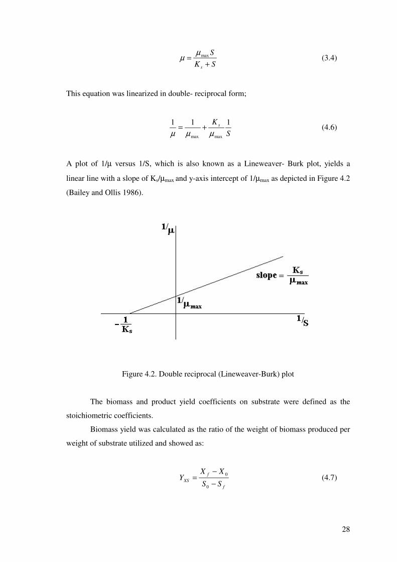
This equation was linearized in double- reciprocal form;
S
K s 111
maxmax µµµ+= (4.6)
A plot of 1/µ versus 1/S, which is also known as a Lineweaver- Burk plot, yields a
linear line with a slope of Ks/µmax and y-axis intercept of 1/µmax as depicted in Figure 4.2
(Bailey and Ollis 1986).
Figure 4.2. Double reciprocal (Lineweaver-Burk) plot
The biomass and product yield coefficients on substrate were defined as the
stoichiometric coefficients.
Biomass yield was calculated as the ratio of the weight of biomass produced per
weight of substrate utilized and showed as:
f
fXS SS
XXY
−−
=0
0 (4.7)
29
Product yield was also defined as the weight of product produced per weight of
substrate utilized and the equation was:
f
fPS SS
PPY
−−
=0
0 (4.8)
The differential equations based on biomass growth, substrate utilization and
product formation were solved numerically by second and third order Runga-Kutta
method. Initial biomass, lactic acid and lactose concentrations within defined time span
were initiate the solution of these differential equations. The initial biomass, substrate
and product concentrations for the fermentation run were given in Table.E.1 in
Appendix E.
The best values of the parameters of the models were adjusted by minimizing
the objective function given as;
�= �
��
��
� �
��
���
� −+�
�
���
� −+�
�
���
� −=
N
i
icaliicaliicali
S
SS
P
PP
X
XXSSE
1
2
max
exp2
max
exp2
max
exp (4.9)
Equation (4.9) is the sum of squares of errors of the model. N is the number of
observations in a single fermentation, and Xmax, Pmax, and Smax are the maximum
biomass, product and substrate concentrations, respectively (Starzak et al. 1994). ‘exp’
subscript is used for the experimental data, ‘cal’ subscript is used for the simulation
results.

CHAPTER 5
RESULTS AND DISCUSSION
5.1. Fermentation Experiments
In the kinetic modelling studies of lactic acid production from whey by L. casei,
seven different fermentation experiments with different initial substrate concentrations
(S0) were performed. These fermentations, with 9.0, 21.4, 35.5, 48.0, 61.2, 77.1, and
95.7 g l-1 initial substrate concentrations, were used to determine kinetic and
stoichiometric parameters such as �max, α, KS, YPS, YXS.
Before each fermentation experiment, whey powder was dissolved in deionized
water to get required concentration. However, using the whey powder solution in the
fermenter directly causes difficulties in the biomass measurements in the UV
spectrophotometer. Therefore, it is necessary to go through a pretreatment procedure of
whey solution before the fermentation starts. The heat treatment can be used to denature
the proteins of whey, which cause the turbidity during the measurements. For this
reason, whey solution was autoclaved at 121oC for 15 min. At high temperature some of
the whey proteins were denatured and formed small particles. Recovery of heat-
precipitated whey proteins was accomplished by a centrifuge. This treatment decreased
the protein amount from 11.15 % to 5.2 % in whey powder. The lactose concentration
of solution was detected before and after pretreatment. The results showed that there is
not any lactose loss with pretreatment.
In these fermentations, the stationary phase was occurred at around 10-12 hours except
the fermentations with 9.0 and 21.4 g l-1 initial substrate concentration. Also, most of
the initial lactic acid came from the inoculum, which was produced during the shake
flask fermentation to be used for the fermenter. The rest of the initial lactic acid came
from the whey used as substrate in the fermenter.
The fermentation with 9.0 g l-1 initial substrate concentration was completed
within 4 hours (Figure 5.1). The biomass concentration was reached to 3.5 g l-1 at the
end of the fermentation. After 4 hours, all lactose was utilized as soon as the stationary
phase was attained. However, it was seen that, 60 % of lactose was converted to lactic

31
acid. The remaining portion of lactose might have been used for cell growth and
maintenance.
0
1
2
3
4
5
6
7
8
9
10
0 0.5 1 1.5 2 2.5 3 3.5 4 4.5
time (h)
lact
ose,
lact
ic a
cid
(g l-1
)
0
1
2
3
4
5
6
7
8
biom
ass
conc
entr
atio
n (g
l-1)
Figure 5.1. Experimental results of fermentation with 9.0 g l-1 initial substrate for
lactose (o), lactic acid (•) and biomass (+)
Similarly, with the initial substrate concentration of 21.4 g l-1, 60 % conversion
of lactose to lactic acid was obtained within 7 hours (Figure 5.2). A similar behaviour as
in the initial substrate of 9.0 g l-1 was observed in this case, too. Within 7 hours, all the
substrate was depleted even the microorganism stopped growing, a small amount of
lactic acid, approximately 2 g l-1, was produced. In this fermentation, the biomass
concentration was approximately 5 g l-1 at the end of the experiment.

32
0
2
4
6
8
10
12
14
16
18
20
22
0 1 2 3 4 5 6 7 8 9
time (h)
lact
ose,
lact
ic a
cid
(g l-1
)
0
1
2
3
4
5
6
7
8
biom
ass
conc
entr
atio
n (g
l-1)
Figure 5.2. Experimental results of fermentation with 21.4 g l-1 initial substrate for
lactose (o), lactic acid (•) and biomass (+).
0
5
10
15
20
25
30
35
40
0 1 2 3 4 5 6 7 8 9 10 11
time (h)
lact
ose,
lact
ic a
cid
(g l-1
)
0
1
2
3
4
5
6
7
8
biom
ass
conc
entr
atio
n (g
l-1)
Figure 5.3. Experimental results of fermentation with 35.5 g l-1 initial substrate for
lactose (o), lactic acid (•) and biomass (+).

33
Another fermentation experiment was performed with the initial substrate
concentration of 35.5 g l-1. In this case, the deceleration and stationary phases were
observed at 8 h and 10 h, respectively (Figure 5.3). In stationary phase, 7 g l-1 biomass
concentration was observed. 53 % of lactose was converted to lactic acid before
deceleration phase and 29 % conversion was achieved in deceleration and stationary
phases. It was seen that, all substrate was consumed at the end of the tenth hour.
In the fermentation with 48.0 g l-1 initial lactose concentration, 50 % of lactose
was converted in the exponential phase and 17 % of it was converted in the deceleration
and stationary phases (Figure 5.4). Similar to 35 g l-1 initial lactose concentration case,
the deceleration and stationary phases were observed at 8 h and 11 h, respectively and
the biomass concentration was 7 g l-1, too. In this experiment, all lactose was utilized
within 14.5 hours.
0
5
10
15
20
25
30
35
40
45
50
0 1 2 3 4 5 6 7 8 9 10 11 12 13 14
time (h)
lact
ose,
lact
ic a
cid
(g l-1
)
0
1
2
3
4
5
6
7
8
biom
ass
conc
entr
atio
n (g
l-1)
Figure 5.4. Experimental results of fermentation with 48.0 g l-1 initial substrate for
lactose (o), lactic acid (•) and biomass (+).
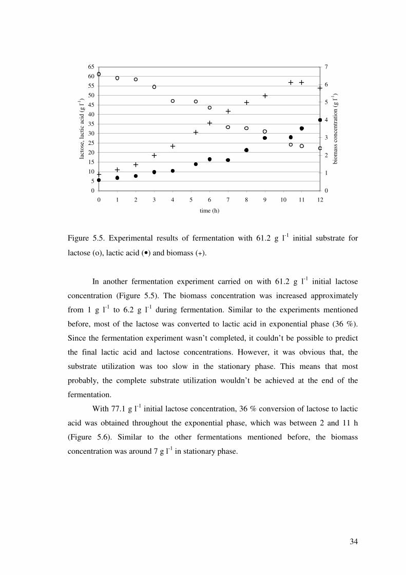
34
0
5
10
15
20
25
30
35
40
45
50
55
60
65
0 1 2 3 4 5 6 7 8 9 10 11 12
time (h)
lact
ose,
lact
ic a
cid
(g l-1
)
0
1
2
3
4
5
6
7
biom
ass
conc
entr
atio
n (g
l-1)
Figure 5.5. Experimental results of fermentation with 61.2 g l-1 initial substrate for
lactose (o), lactic acid (•) and biomass (+).
In another fermentation experiment carried on with 61.2 g l-1 initial lactose
concentration (Figure 5.5). The biomass concentration was increased approximately
from 1 g l-1 to 6.2 g l-1 during fermentation. Similar to the experiments mentioned
before, most of the lactose was converted to lactic acid in exponential phase (36 %).
Since the fermentation experiment wasn’t completed, it couldn’t be possible to predict
the final lactic acid and lactose concentrations. However, it was obvious that, the
substrate utilization was too slow in the stationary phase. This means that most
probably, the complete substrate utilization wouldn’t be achieved at the end of the
fermentation.
With 77.1 g l-1 initial lactose concentration, 36 % conversion of lactose to lactic
acid was obtained throughout the exponential phase, which was between 2 and 11 h
(Figure 5.6). Similar to the other fermentations mentioned before, the biomass
concentration was around 7 g l-1 in stationary phase.

35
0
10
20
30
40
50
60
70
80
0 1 2 3 4 5 6 7 8 9 10 11 12 13 14 15
time (h)
lact
ose,
lact
ic a
cid
(g l-1
)
0
1
2
3
4
5
6
7
8
biom
ass
conc
entr
atio
n (g
l-1)
Figure 5.6. Experimental results of fermentation with 77.1 g l-1 initial substrate for
lactose (o), lactic acid (•) and biomass (+).
As expected, the concentration of residual lactose decreased during the
fermentation with 95.7 g l-1 initial lactose concentration (Figure 5.7). This coincided
with an increase in lactic acid production. The concentration of residual lactose fell
rapidly during the first 24 hours of fermentation after slow decrease. 31 % conversion of
lactose to lactic acid was achieved during exponential phase within 11 hours. Nearly
same amount of lactic acid was produced during the deceleration and stationary phases.
However, it took more than 22 hours. As a result, the high initial substrate
concentrations caused lower yields in very long fermentation time. So, it might be
concluded that the fermentations with high initial lactose concentrations are not
economical in industrial productions.
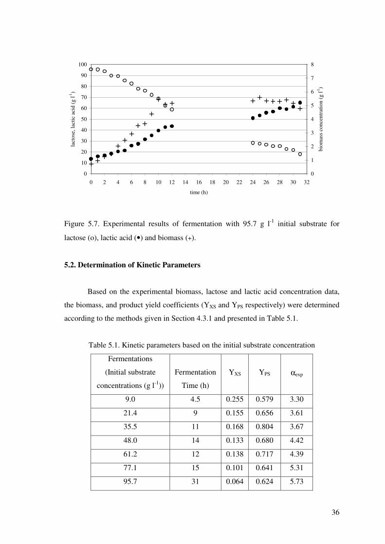
36
0
10
20
30
40
50
60
70
80
90
100
0 2 4 6 8 10 12 14 16 18 20 22 24 26 28 30 32
time (h)
lact
ose,
lact
ic a
cid
(g l-1
)
0
1
2
3
4
5
6
7
8
biom
ass
conc
entr
atio
n (g
l-1)
Figure 5.7. Experimental results of fermentation with 95.7 g l-1 initial substrate for
lactose (o), lactic acid (•) and biomass (+).
5.2. Determination of Kinetic Parameters
Based on the experimental biomass, lactose and lactic acid concentration data,
the biomass, and product yield coefficients (YXS and YPS respectively) were determined
according to the methods given in Section 4.3.1 and presented in Table 5.1.
Table 5.1. Kinetic parameters based on the initial substrate concentration
Fermentations
(Initial substrate
concentrations (g l-1))
Fermentation
Time (h)
YXS
YPS
αexp
9.0 4.5 0.255 0.579 3.30
21.4 9 0.155 0.656 3.61
35.5 11 0.168 0.804 3.67
48.0 14 0.133 0.680 4.42
61.2 12 0.138 0.717 4.39
77.1 15 0.101 0.641 5.31
95.7 31 0.064 0.624 5.73

37
The product yield on substrate, YPS, changes with different initial substrate
concentrations in a narrow range (Figure 5.8). For this reason, the average value of
calculated product yield was taken as 0.682 in the model development
.
00.10.20.30.40.50.60.70.80.9
0 20 40 60 80 100 120
Initial substrate concentration (g l-1)
Prod
uct y
ield
on
subs
trat
e, Y
PS
Figure 5.8. Relation between the product yield coefficient and initial substrate
concentration.
However, the biomass yield on substrate, YXS followed a different trend. The
biomass yield decreased with the increase in the initial substrate concentration. The
relationship between the biomass yield coefficient and the initial substrate concentration
could be clearly seen in Figure 5.9.

38
y = -0.0018x + 0.2334
0
0.05
0.1
0.15
0.2
0.25
0.3
0 20 40 60 80 100
Initial substrate concentration (g l-1)
Bio
mas
s yi
eld
on s
ubst
rate
, YX
S
Figure 5.9. Relationship between the biomass yield coefficient, YXS, and initial substrate
concentration, S0.
Table 5.1 also presents the experimental α values (αexp). α is the growth-
associated term parameter in the Leudeking-Piret equation:
XdtdX
dtdP βα += (3.5)
In the study of Amrane and Prigent in 1997, more confident conclusions were
reached when the coefficient of Luedeking-Piret equation, α, was calculated from the
equation below:
)()( 00 XXPP −=− α (5.1)
The α values in Table 5.1 were calculated by using the experimental lactic acid
and biomass concentration data in Equation (5.1). The results showed that there was a
linear relationship between α and the initial lactose concentrations. In Figure 5.10, it is
obviously seen that α increased with the increase in initial substrate concentration.
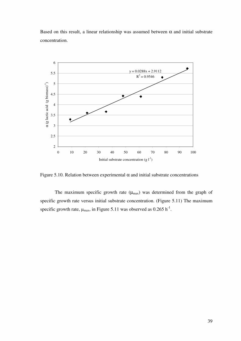
39
Based on this result, a linear relationship was assumed between α and initial substrate
concentration.
Figure 5.10. Relation between experimental α and initial substrate concentrations
The maximum specific growth rate (µmax) was determined from the graph of
specific growth rate versus initial substrate concentration. (Figure 5.11) The maximum
specific growth rate, �max, in Figure 5.11 was observed as 0.265 h-1.
y = 0.0288x + 2.9112R2 = 0.9546
2
2.5
3
3.5
4
4.5
5
5.5
6
0 10 20 30 40 50 60 70 80 90 100
Initial substrate concentration (g l-1)
α (g
lact
ic a
cid
(g b
iom
ass)
-1)
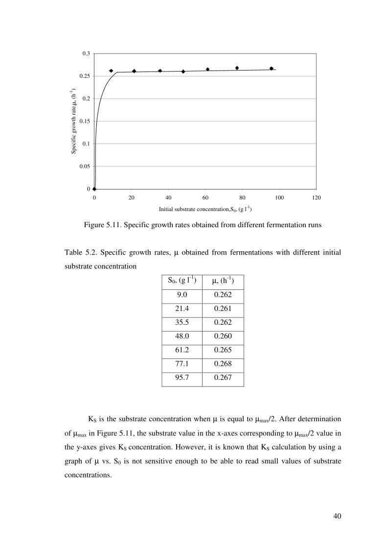
40
0
0.05
0.1
0.15
0.2
0.25
0.3
0 20 40 60 80 100 120
Initial substrate concentration,S0, (g l-1)
Spec
ific
gro
wth
rate
, µ, (
h-1)
Figure 5.11. Specific growth rates obtained from different fermentation runs
Table 5.2. Specific growth rates, µ obtained from fermentations with different initial
substrate concentration
S0, (g l-1) µ, (h-1)
9.0 0.262
21.4 0.261
35.5 0.262
48.0 0.260
61.2 0.265
77.1 0.268
95.7 0.267
KS is the substrate concentration when µ is equal to µmax/2. After determination
of µmax in Figure 5.11, the substrate value in the x-axes corresponding to µmax/2 value in
the y-axes gives KS concentration. However, it is known that KS calculation by using a
graph of µ vs. S0 is not sensitive enough to be able to read small values of substrate
concentrations.
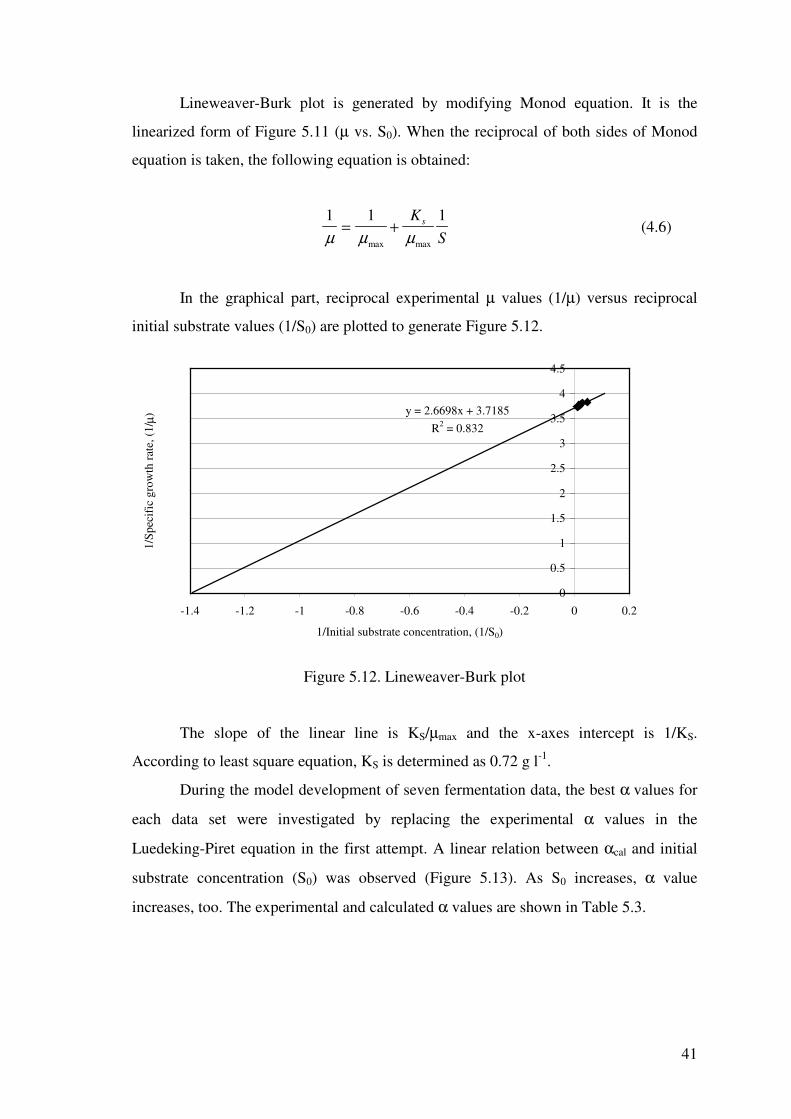
41
Lineweaver-Burk plot is generated by modifying Monod equation. It is the
linearized form of Figure 5.11 (µ vs. S0). When the reciprocal of both sides of Monod
equation is taken, the following equation is obtained:
S
Ks 111
maxmax µµµ+= (4.6)
In the graphical part, reciprocal experimental µ values (1/µ) versus reciprocal
initial substrate values (1/S0) are plotted to generate Figure 5.12.
y = 2.6698x + 3.7185R2 = 0.832
0
0.5
1
1.5
2
2.5
3
3.5
4
4.5
-1.4 -1.2 -1 -0.8 -0.6 -0.4 -0.2 0 0.2
1/Initial substrate concentration, (1/S0)
1/Sp
ecif
ic g
row
th ra
te, (
1/µ)
Figure 5.12. Lineweaver-Burk plot
The slope of the linear line is KS/µmax and the x-axes intercept is 1/KS.
According to least square equation, KS is determined as 0.72 g l-1.
During the model development of seven fermentation data, the best α values for
each data set were investigated by replacing the experimental α values in the
Luedeking-Piret equation in the first attempt. A linear relation between αcal and initial
substrate concentration (S0) was observed (Figure 5.13). As S0 increases, α value
increases, too. The experimental and calculated α values are shown in Table 5.3.
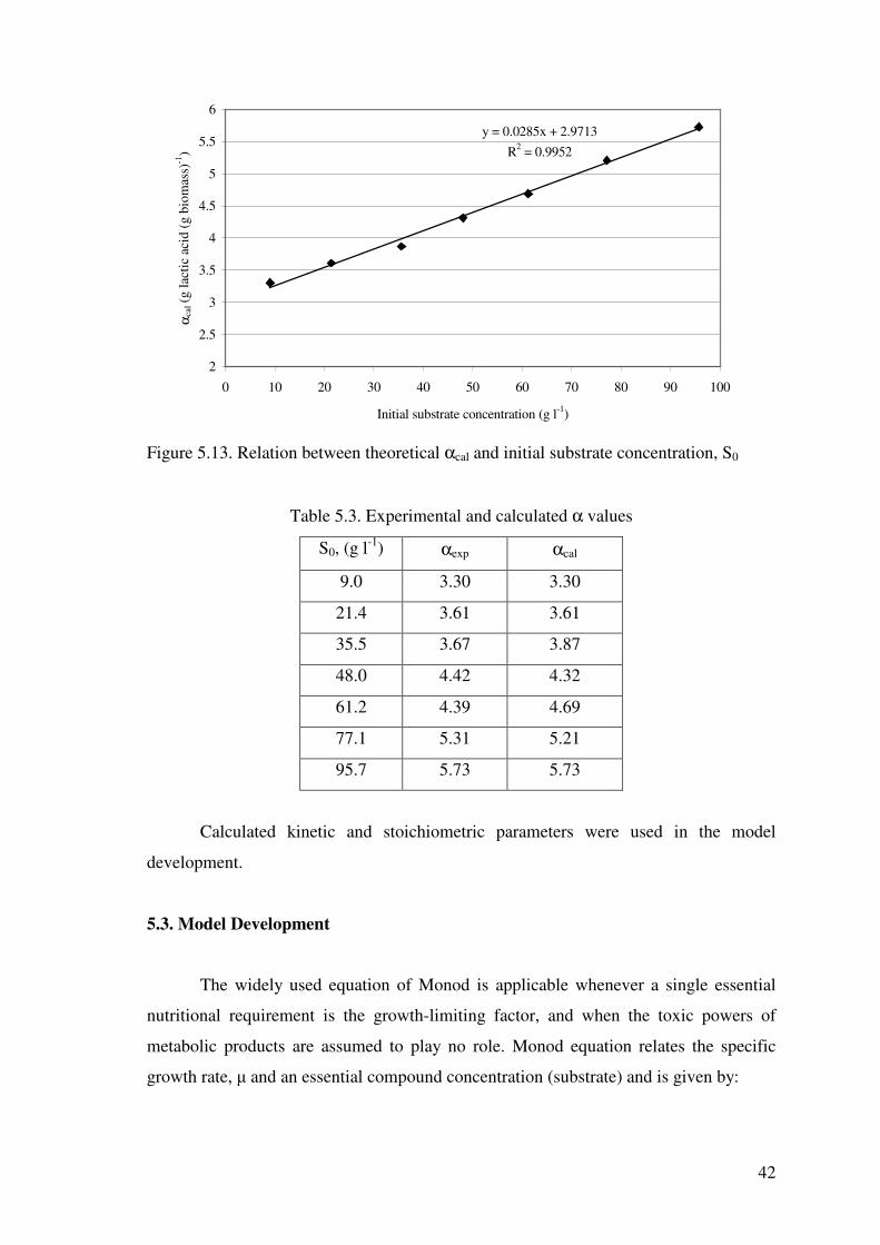
42
Figure 5.13. Relation between theoretical αcal and initial substrate concentration, S0
Table 5.3. Experimental and calculated α values
S0, (g l-1) αexp αcal
9.0 3.30 3.30
21.4 3.61 3.61
35.5 3.67 3.87
48.0 4.42 4.32
61.2 4.39 4.69
77.1 5.31 5.21
95.7 5.73 5.73
Calculated kinetic and stoichiometric parameters were used in the model
development.
5.3. Model Development
The widely used equation of Monod is applicable whenever a single essential
nutritional requirement is the growth-limiting factor, and when the toxic powers of
metabolic products are assumed to play no role. Monod equation relates the specific
growth rate, � and an essential compound concentration (substrate) and is given by:
y = 0.0285x + 2.9713R2 = 0.9952
2
2.5
3
3.5
4
4.5
5
5.5
6
0 10 20 30 40 50 60 70 80 90 100
Initial substrate concentration (g l-1)
α cal (g
lact
ic a
cid
(g b
iom
ass)
-1)
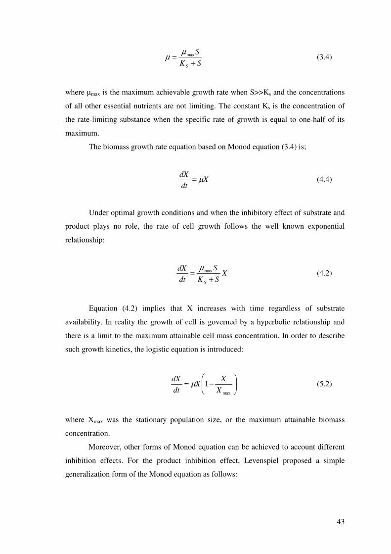
43
SKS
S += maxµµ (3.4)
where �max is the maximum achievable growth rate when S>>Ks and the concentrations
of all other essential nutrients are not limiting. The constant Ks is the concentration of
the rate-limiting substance when the specific rate of growth is equal to one-half of its
maximum.
The biomass growth rate equation based on Monod equation (3.4) is;
XdtdX µ= (4.4)
Under optimal growth conditions and when the inhibitory effect of substrate and
product plays no role, the rate of cell growth follows the well known exponential
relationship:
XSKS
dtdX
S += maxµ
(4.2)
Equation (4.2) implies that X increases with time regardless of substrate
availability. In reality the growth of cell is governed by a hyperbolic relationship and
there is a limit to the maximum attainable cell mass concentration. In order to describe
such growth kinetics, the logistic equation is introduced:
���
����
�−=
max
1X
XX
dtdX µ (5.2)
where Xmax was the stationary population size, or the maximum attainable biomass
concentration.
Moreover, other forms of Monod equation can be achieved to account different
inhibition effects. For the product inhibition effect, Levenspiel proposed a simple
generalization form of the Monod equation as follows:
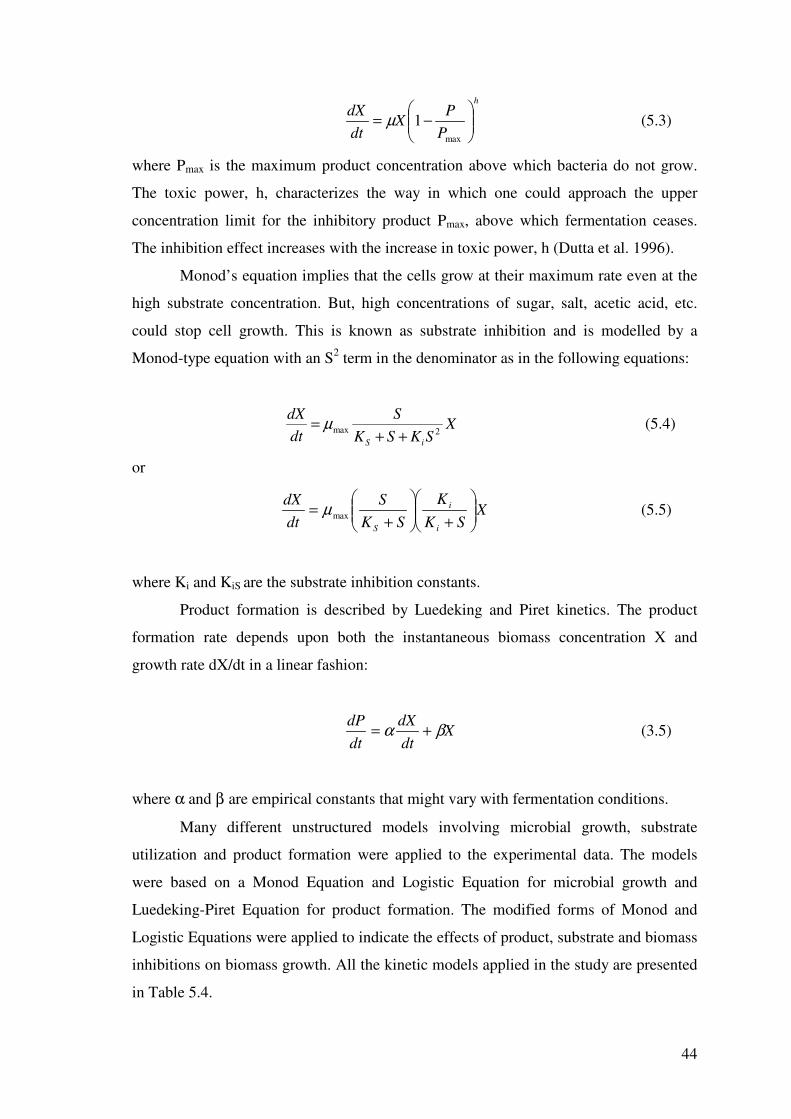
44
h
PP
XdtdX
���
����
�−=
max
1µ (5.3)
where Pmax is the maximum product concentration above which bacteria do not grow.
The toxic power, h, characterizes the way in which one could approach the upper
concentration limit for the inhibitory product Pmax, above which fermentation ceases.
The inhibition effect increases with the increase in toxic power, h (Dutta et al. 1996).
Monod’s equation implies that the cells grow at their maximum rate even at the
high substrate concentration. But, high concentrations of sugar, salt, acetic acid, etc.
could stop cell growth. This is known as substrate inhibition and is modelled by a
Monod-type equation with an S2 term in the denominator as in the following equations:
XSKSK
SdtdX
iS2max ++
= µ (5.4)
or
XSK
KSK
SdtdX
i
i
S���
����
�
+���
����
�
+= maxµ (5.5)
where Ki and KiS are the substrate inhibition constants.
Product formation is described by Luedeking and Piret kinetics. The product
formation rate depends upon both the instantaneous biomass concentration X and
growth rate dX/dt in a linear fashion:
XdtdX
dtdP βα += (3.5)
where α and β are empirical constants that might vary with fermentation conditions.
Many different unstructured models involving microbial growth, substrate
utilization and product formation were applied to the experimental data. The models
were based on a Monod Equation and Logistic Equation for microbial growth and
Luedeking-Piret Equation for product formation. The modified forms of Monod and
Logistic Equations were applied to indicate the effects of product, substrate and biomass
inhibitions on biomass growth. All the kinetic models applied in the study are presented
in Table 5.4.

45
Table 5.4. Models applied in the study
Model Number
Biomass Growth
Product Formation
Substrate Utilization
Model 1
XdtdX µ=
XdtdX
dtdP βα +=
XmdtdP
YdtdX
YdtdS
SPSXS
−−−=11
Model 2
h
PmP
XdtdX
��
���
� −= 1µ
XdtdX
dtdP βα +=
XmdtdP
YdtdS
SPS
−−= 1
Model 3
( )hPXdtdX −= expµ
XdtdX
dtdP βα +=
XmdtdP
YdtdS
SPS
−−= 1
Model 4
XSK
KdtdX
i
i���
����
�
+= µ
XdtdX
dtdP βα +=
XmdtdP
YdtdS
SPS
−−= 1
Model 5
( )XKPKSSK
SdtdX
PiS
/exp/2max −
++= µ
XdtdX
dtdP βα +=
XmdtdP
YdtdS
SPS
−−= 1
45
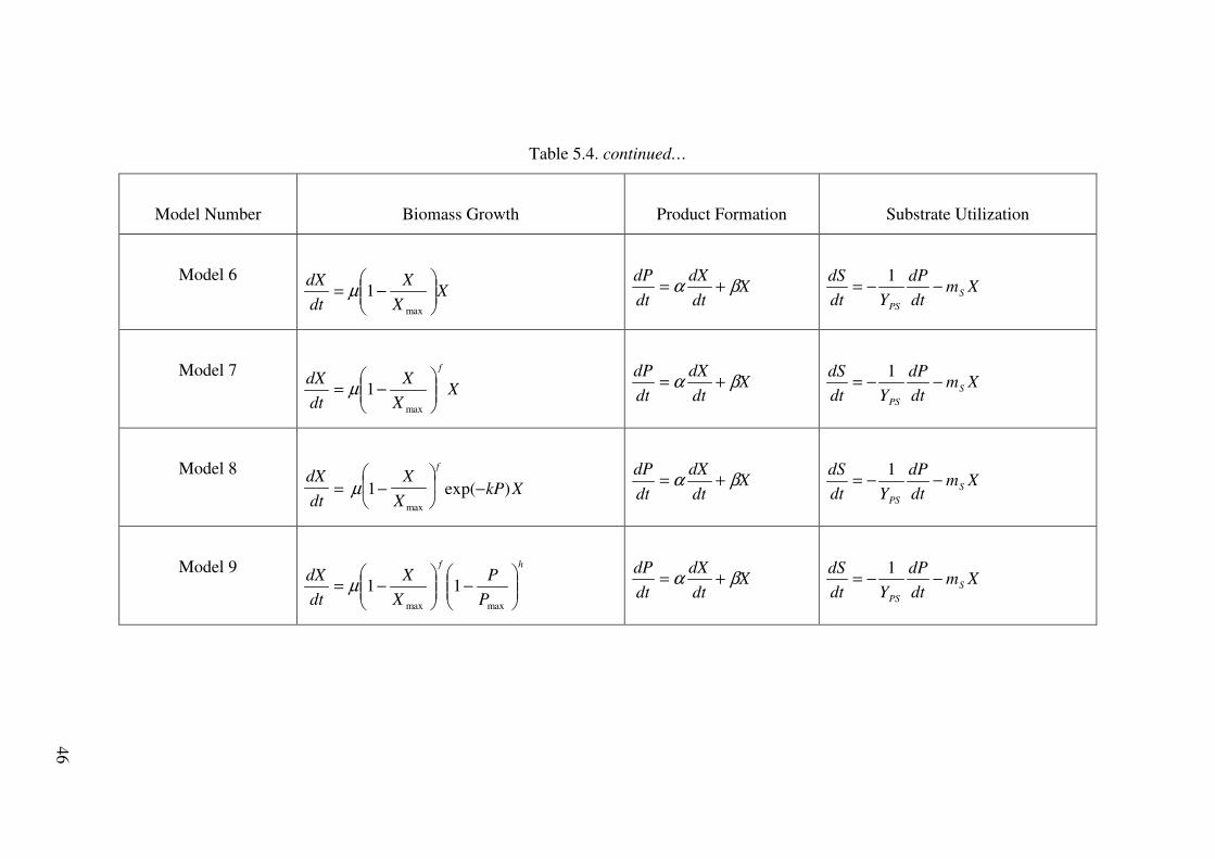
46
Table 5.4. continued…
Model Number
Biomass Growth
Product Formation
Substrate Utilization
Model 6
XX
XdtdX
���
����
�−=
max
1µ
XdtdX
dtdP βα +=
XmdtdP
YdtdS
SPS
−−= 1
Model 7
XX
XdtdX
f
���
����
�−=
max
1µ
XdtdX
dtdP βα +=
XmdtdP
YdtdS
SPS
−−= 1
Model 8
XkPX
XdtdX
f
)exp(1max
−��
���
�−= µ
XdtdX
dtdP βα +=
XmdtdP
YdtdS
SPS
−−= 1
Model 9
hf
PP
XX
dtdX
���
����
�−��
�
����
�−=
maxmax
11µ
XdtdX
dtdP βα +=
XmdtdP
YdtdS
SPS
−−= 1
46

47
In these models, the product inhibition was assumed as following the linear or
exponential fashion. The kinetics of inhibition due to high substrate concentration
depends on the type of substrate and microorganism. It is usually described by an
exponential or hyperbolic dependence (Starzak et al. 1994). The hyperbolic substrate
inhibition case was applied in this study. In processes involving a high concentration of
microbial cells, the biomass itself also inhibits growth and product formation. This was
represented by a term proportional to the biomass concentration.
The models have been developed under the assumption that the observed change
in cell mass results from the growth process only, neglecting both endogenous
metabolism and cell death. Thus, the biomass growth rate was described by the Monod
Equation;
XSK
SdtdX
S += maxµ (4.2)
Additionally, the Luedeking- Piret equation (3.5) to explain the product
formation was used in the first attempt. In that case, the substrate utilization was
expressed as:
XmdtdP
YdtdX
YdtdS
SPSXS
−−−= 11 (4.3)
A very high value of sum of errors (SSE range is 1.61-3.02) was obtained in
Model 1 (Table 5.4). Sudden depletion in substrate concentration promised neither
biomass nor product to reach actual values (App. D Figure D.1). This could be caused
by a very small value of YXS, which yields a substrate concentration mostly to biomass
growth instead of product formation.
Based on the result of Model 1, the equation of substrate utilization rate was
changed by considering the conversion to product and maintenance for biomass growth
as Equation (5.6). In the production of lactic acid, the cell dissimilates substrate to lactic
acid in order to obtain the energy required to form new bacterial protoplasm. At the
same time, it performs its normal metabolic activity irrespective of growth. It might,
therefore, be presumed that a portion of substrate is used for maintenance of the cell
during fermentation. The substrate utilization kinetics given by equation (5.6), which

48
was used in the studies of Biazar et al. 2003 and Dutta et al. 1996, considered substrate
conversion to product and substrate consumption for maintenance:
XmdtdP
YdtdS
SPS
−−= 1 (5.6)
Also, the biomass growth rate equation was modified by the addition of product
inhibition term:
h
PP
XdtdX
���
����
�−=
max
1µ (5.3)
where Pmax is the maximum product concentration above which bacteria do not grow
and h is the toxic power. This approach may be linear when h is unity or there is a rapid
initial drop in production rate followed by a slow approach to Pmax when h>1.
Luedeking and Piret Equation (3.5) was used to describe lactic acid formation rate in
Model 2. The results of Model 2 were seen in Figure D.2 in Appendix D.
In the experiments with high initial substrate concentrations such as 95.696
g l-1and 77.122 g l-1, there wasn’t a significant change in sum of squares of errors
conforming the important role that product inhibition plays in the process of lactic acid
fermentation. However, the product formation of low initial substrate concentration
experiments such as 9.014 g l-1 and 21.438 g l-1, could be explained better with higher
accuracy (SSE is 0.86 and 0.55, respectively).
In Model 3, the product inhibition term was changed to exponential inhibition
term (Table 5.4). Similar results were obtained with previous model (App. D Figure
D.3). There was not a good agreement in the model simulations and experimental data
of the biomass growth in the experiments with low initial substrate concentrations. The
reason for this result might be the sudden decrease in the substrate concentration, low
increase in product and biomass concentrations. To overcome this problem, the
substrate inhibition terms were introduced to Monod Equation and applied as Equation
(5.4) and Equation (5.5) (Model 4 and Model 5, respectively). Unexpectedly, the
inhibition effect was too strong that all concentrations obtained from the model
simulations were lower values than the experimental concentrations. The results of

49
Model 4 and Model 5 were seen in Figure D.4 and Figure D.5 in Appendix D,
respectively.
Monod Equation defines the biomass growth rate as an exponential relationship.
In reality the growth of cell is governed by a hyperbolic relationship and there is a limit
to the maximum achievable cell mass concentration. The Logistic Equation describes
such growth kinetics representing both an exponential and stationary phases. From the
point of view of data fitting, Model 6 produced lower value of SSE than the previous
models did (App. D Figure D.6). In addition, the Logistic Equation was modified with
toxic power (f), to adopt the model to the wide range of initial substrate concentration
experiments as given in Equation (5.7) and the results were shown in Figure D.7 in
Appendix D (Model 7):
XX
XdtdX
f
���
����
�−=
max
1µ (5.7)
On the other hand, since the effect of product inhibition is considerable for lactic
acid fermentation, the modification of Logistic Equation with product inhibition term
might give better agreement of model predictions with the experimental data. For this
reason, exponential product inhibition term (5.8) and Levenspiel product inhibition term
(5.9) were used in models 8 and 9, respectively (Table 5.6).
XkPX
XdtdX
f
)exp(1max
−��
���
�−= µ (5.8)
hf
PP
XX
dtdX
���
����
�−��
�
����
�−=
maxmax
11µ (5.9)
The result of Model 8 was seen in Figure D.8 in Appendix D.
The Logistic Equation modified with biomass and product inhibition terms
produced lower values of the sum of squares of errors. The use of Equation (5.9) was
more applicable to the wide range of initial substrate concentration fermentations since
the toxic powers define the power of the inhibition and vary for the extreme cases such
as a very low and very high initial substrate concentrations, 9.0 and 96 g l-1, respectively
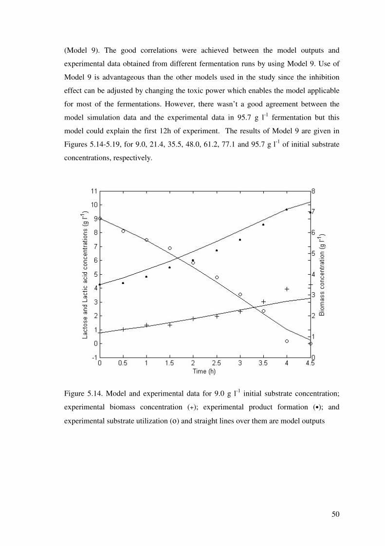
50
(Model 9). The good correlations were achieved between the model outputs and
experimental data obtained from different fermentation runs by using Model 9. Use of
Model 9 is advantageous than the other models used in the study since the inhibition
effect can be adjusted by changing the toxic power which enables the model applicable
for most of the fermentations. However, there wasn’t a good agreement between the
model simulation data and the experimental data in 95.7 g l-1 fermentation but this
model could explain the first 12h of experiment. The results of Model 9 are given in
Figures 5.14-5.19, for 9.0, 21.4, 35.5, 48.0, 61.2, 77.1 and 95.7 g l-1 of initial substrate
concentrations, respectively.
Figure 5.14. Model and experimental data for 9.0 g l-1 initial substrate concentration;
experimental biomass concentration (+); experimental product formation (•); and
experimental substrate utilization (ο) and straight lines over them are model outputs

51
Figure 5.15. Model and experimental data for 21.4 g l-1 initial substrate concentration;
experimental biomass concentration (+); experimental product formation (•); and
experimental substrate utilization (ο) and straight lines over them are model outputs
Figure 5.16. Model and experimental data for 35.5 g l-1 initial substrate concentration;
experimental biomass concentration (+); experimental product formation (•); and
experimental substrate utilization (ο) and straight lines over them are model outputs

52
Figure 5.17. Model and experimental data for 48.0 g l-1 initial substrate concentration;
experimental biomass concentration (+); experimental product formation (•); and
experimental substrate utilization (ο) and straight lines over them are model outputs.
Figure 5.18. Model and experimental data for 61.2 g l-1 initial substrate concentration;
experimental biomass concentration (+); experimental product formation (•); and
experimental substrate utilization (ο) and straight lines over them are model outputs
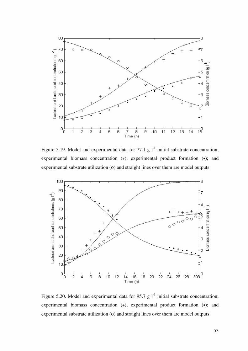
53
Figure 5.19. Model and experimental data for 77.1 g l-1 initial substrate concentration;
experimental biomass concentration (+); experimental product formation (•); and
experimental substrate utilization (ο) and straight lines over them are model outputs
Figure 5.20. Model and experimental data for 95.7 g l-1 initial substrate concentration;
experimental biomass concentration (+); experimental product formation (•); and
experimental substrate utilization (ο) and straight lines over them are model outputs
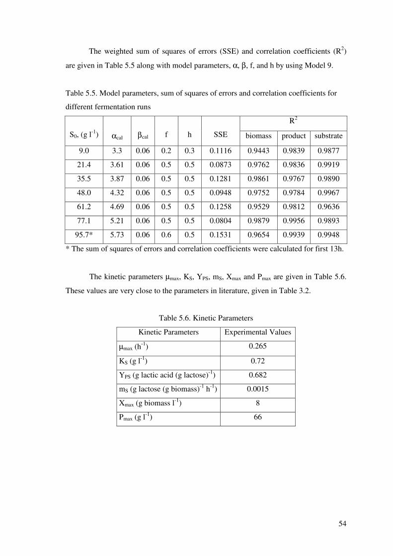
54
The weighted sum of squares of errors (SSE) and correlation coefficients (R2)
are given in Table 5.5 along with model parameters, α, β, f, and h by using Model 9.
Table 5.5. Model parameters, sum of squares of errors and correlation coefficients for
different fermentation runs
R2
S0, (g l-1)
αcal
βcal
f
h
SSE biomass product substrate
9.0 3.3 0.06 0.2 0.3 0.1116 0.9443 0.9839 0.9877
21.4 3.61 0.06 0.5 0.5 0.0873 0.9762 0.9836 0.9919
35.5 3.87 0.06 0.5 0.5 0.1281 0.9861 0.9767 0.9890
48.0 4.32 0.06 0.5 0.5 0.0948 0.9752 0.9784 0.9967
61.2 4.69 0.06 0.5 0.5 0.1258 0.9529 0.9812 0.9636
77.1 5.21 0.06 0.5 0.5 0.0804 0.9879 0.9956 0.9893
95.7* 5.73 0.06 0.6 0.5 0.1531 0.9654 0.9939 0.9948
* The sum of squares of errors and correlation coefficients were calculated for first 13h.
The kinetic parameters µmax, KS, YPS, mS, Xmax and Pmax are given in Table 5.6.
These values are very close to the parameters in literature, given in Table 3.2.
Table 5.6. Kinetic Parameters
Kinetic Parameters Experimental Values
µmax (h-1) 0.265
KS (g l-1) 0.72
YPS (g lactic acid (g lactose)-1) 0.682
mS (g lactose (g biomass)-1 h-1) 0.0015
Xmax (g biomass l-1) 8
Pmax (g l-1) 66

55
5.4. Productivity of the Fermentation Runs
The productivity values calculated with the experimental data in exponential
phase were plotted against initial substrate concentrations as in Figure 5.21. The
productivity values were calculated by the equation given below:
Productivity =0
0
tt
PP
f
f
−−
(5.10)
Figure 5.21. Productivity from experimental data in exponential phase
This plot indicates that the productivity remains constant at certain amount of
initial substrate concentration. Actually, better explanation for productivity can be
achieved by the complete substrate utilization. However, in this study, some of the
fermentations were carried out without the utilization of all substrate. Thus, the product
values when the substrate is zero were predicted by the model simulations by using
Model 9. According to the prediction values of product, the plot of predicted
productivity versus initial substrate was obtained as in Figure 5.22.
0
0.5
1
1.5
2
2.5
3
0 10 20 30 40 50 60 70 80 90 100
S0 (g l-1)
Prod
uctiv
ity (g
l-1 h-1
)
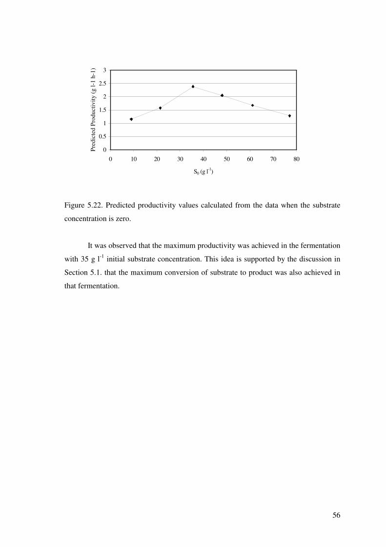
56
Figure 5.22. Predicted productivity values calculated from the data when the substrate
concentration is zero.
It was observed that the maximum productivity was achieved in the fermentation
with 35 g l-1 initial substrate concentration. This idea is supported by the discussion in
Section 5.1. that the maximum conversion of substrate to product was also achieved in
that fermentation.
0
0.5
1
1.5
2
2.5
3
0 10 20 30 40 50 60 70 80
S0 (g l-1)
Pred
icte
d Pr
oduc
tivity
(g l-
1 h-
1)
CHAPTER 6
CONCLUSIONS AND RECOMMENDATIONS
The fermentation of whey lactose by Lactobacillus casei to produce lactic acid,
which is a widely used organic acid, was modelled by kinetic equations of biomass
growth, product formation and substrate consumption.
The kinetic parameters of lactic acid productions were determined by series of
batch fermentation experiments with seven different initial lactose concentrations in a
range from 9.0 g l-1 to 95.7 g l-1. The maximum specific growth rate, µmax, was obtained
as 0.265 h-1. The Monod constant, KS, was calculated from the Lineweaver-Burk plot as
0.72 g l-1. The product on substrate yield values were very close in different
fermentations, so the average value of 0.682 was used in models.
In the model development part, initially different model equations were used
such as Monod and logistic equations for biomass growth, and Luedeking and Piret
equation for product formation. The substrate utilization rate equation was based on the
substrate utilized for product formation, biomass growth and maintenance. Also, the
equation for specific growth rate was modified by including a product inhibition and
substrate inhibition terms. It was seen that, the addition of biomass and product
inhibition terms promised a better fit of the model simulation data to the experimental
data. The rate equations including biomass growth, lactic acid production and lactose
utilization were solved numerically by Runga-Kutta method.
By using modified logistic equation with product inhibition term for biomass
growth, Luedeking and Piret equation for product formation and substrate consumption
equation for product formation and maintenance, the most reliable and applicable model
was developed. The toxic powers in these inhibition terms made the model applicable
for the fermentation experiments with low and high initial substrate concentrations
when the inhibition effects became negligible and significant, respectively.
In further studies the effect of pH and temperature on kinetic parameters should
be investigated and included in kinetic models. Moreover, the model used in this study
(Model 9) should be developed in order to express the fermentations with high substrate
concentrations better. Also, if this unstructured model could be gathered with the
structured model then the growth kinetics of a culture would be completely described. A

58
chemically structured model divides the cell mass into components. If the ratio of these
components change in response to disturbances in the extracellular environment, then
the model behaves analogously to a cell changing its composition in response to
environmental changes.

REFERENCES
Akerberg C., Hofvendahl K., Zacchi G., “Modelling the influence of pH, temperature, glucose and lactic acid concentrations on the kinetics of lactic acid production by Lactococcus lactis ssp. lactis ATCC 19435 in whole-wheat flour,” Applied microbiology and biotechnology, 49, (1998), 682-690
Amrane A., “Batch cultures of supplemented whey permeate using Lactobacillus
helveticus: unstructured model for biomass formation, substrate consumption and lactic acid production,” Enzyme and microbial technology, 28, (2001), 827-834
Amrane A., Prigent Y., “Growth and lactic acid production coupling for Lactobacillus
helveticus cultivated on supplemented whey: influence of peptidic nitrogen deficiency,” Journal of biotechnology, 55, (1997), 1-8
Arellano I., Martinez G., “Optimization of the green fluorescent protein (GFP)
expression from a lactose-inducible promoter in Lactobacillus casei,” FEMS microbiology letters, 10951, (2003), 1-5
Bailey J. E., Ollis D. F., Biochemical engineering fundamentals (McGraw-Hill, Inc.,
USA, 1986) p.385 Bains W., Biotechnology from A to Z (Oxfrod University Pr., Oxford, 1993) Biazar J., Tango M., Babolian E., Islam R., “Solution of the kinetic modelling of lactic
acid fermentation using Adomian decomposition method,” Applied mathematics and computation, 144, (2003), 433-439
Boonmee M., Leksawasdi N., Bridge W., Rogers P. L., “Batch and continuous culture
of Lactococcus lactis NZ133: experimental data and model development,” Biochemical engineering journal, 3672, (2003), 1-9
Büyükkileci, A. O., “L(+) lactic acid production from whey by Lactobacillus casei
NRRL B-441”, MSc., Thesis study, �zmir Institute of Technology, (2000) Carrillo G. E., Roberts P. D., Becerra V. M., “Genetic algorithms for optimal control of
beer fermentation,” IEEE International Symposium on Intelligent Control, Mexico City, Mexico, 2001, p. 391-396
Clark W. S., Concentrated and Dry Milks and Whey, In Applied dairy microbiology,
edited by Elmer H. Marth, James L. Steele (Marcel Dekker, Inc, New York, 1998) p. 76
Cogan T. M., Accolas J. P., Dairy Starter Cultures (VCH Publishers, New York, 1996) Dutta S.K., Mukherjee A., Chakraborty P., “Effect of product inhibition on lactic acid
fermentation: simulation and modelling,” Applied microbiology and biotechnology, 46, (1996), 410-413
60
Frank J. F., Hassan A. N., Starter Cultures and Their Use, In Applied dairy
microbiology, edited by Elmer H. Marth, James L. Steele (Marcel Dekker, Inc, New York, 1998) p. 135
Fu W., Mathews A. P., “Lactic aid production from lactose by Lactobacillus plantarum:
kinetic model and effects of pH, substrate, and oxygen,” Biochemical engineering journal, 3, (1999), 163-170
Henning D. R., Fermented By-Products, In Applied dairy microbiology, edited by Elmer
H. Marth, James L. Steele (Marcel Dekker, Inc, New York, 1998) p. 251-258 Hui Y. H., Khachatourians G. G., Food Biotechnology microorganisms (Wiley-VCH,
Inc, Canada, 1995) p. 247-260 Irvine D. M., Hill A. R., Cheese Technology, In Comprehensive biotechnology, vol. 3
edited by M. Moo-Young (Pergamon Press, 1985) p. 548-550 Kwon S., Yoo I., Lee W. G., Chang H. N., Chang Y. K., “High-rate continuous
production of lactic acid by Lactobacillus rhamnosus in a two-stage membrane cell-recycle bioreactor,” Biotechnology and bioengineering, 73, (2001), 25-34
Kulozik U., Wilde J., “Rapid lactic acid production at high cell concentrations in whey
ultrafiltrate by Lactobacillus helveticus,” Enzyme and microbial technology, 24, (1999), 297-302
Luedeking R., Piret E. L., “A kinetic study of the lactic acid fermentation. Batch
process at controlled pH,” Journal of biotechemical and microbiological technology, 4, (1959), 393-412
Marth E. H., “Utilization of whey through fermentations,” Marschall Italian & Specialty
Cheese Seminars, 1973 McNeil B., Harvey L. M., Fermentation-a practical approach (Oxford University
Press, England, 1990) Messens W., Verluyten J., Leroy F., Vuyst L. D., “Modelling growth and bacteriocin
production by Lactobacillus curvatus LTH 1174 in response to temperature and pH values used for European sausage fermentation processes,” International journal of food microbiology, 81, (2002), 41-52
Montreagudo J. M., Rodriguez L., Rincon J., Fuertes J., “Kinetics of lactic acid
fermentation by Lactobacillus delbrueckii grown on beet molasses,” J. Chem. Tech. Biotechnol., 68, (1997), 271-276
Perez-Arellano I., Perez-Martinez G., “Optimization of the green fluorescent protein
(GFP) expression from a lactose-inducible promoter in Lactobacillus casei,” FEMS microbiology letters, 10951, (2003), 1-5
61
Polat, Z., “L(+) lactic acid purification from fermentation broth using ion exchange resins”, MSc., Thesis study, �zmir Institute of Technology, (2002)
Prescott L. M., Microbiology (Vm. C. Brown Publishers, USA, 1996) Roukas T., Kotzekidou P., “Lactic acid production from deproteinized whey by mixed
cultures of free and coimmobilized Lactobacillus casei and Lactococcus lactis cells using fedbatch culture,” Enzyme and microbial technology, 22, (1998), 199-204
Schepers A.W., Thibauld J., Lacroix C., “Lactobacillus helveticus growth and lactic
acid production during pH-controlled batch cultures in whey permeate/yeast extract medium. Part I. multiple factor kinetic analysis,” Enzyme and microbial technology, 30, (2002), 176-186
Schepers A.W., Thibauld J., Lacroix C., “Lactobacillus helveticus growth and lactic
acid production during pH-controlled batch cultures in whey permeate/yeast extract medium. Part II. kinetic modelling and model validation,” Enzyme and microbial technology, 30, (2002), 187-194
Shuler M. L., Kargi F., Bioprocess engineering basic concepts (Prentice-Hall, Inc.,
USA, 2002) Sinclair C. G., Kristiansen B., “Mathematical models,” In Fermentation kinetics and
modelling, edited by J. D. Bu’Lock (Open University Press, USA, 1987) Starzak M., Krzystek L., Nowicki L., Michalski H., “Macroapproach kinetics of ethanol
fermentation by Saccharomyces cerevisiae: experimental studies and mathematical modeling,” The chemical engineering journal, 54, (1994), 221-240
Tango M. S. A., Ghaly A. E., “Effect of temperature on lactic acid production from
cheese whey using Lactobacillus helveticus under batch conditions,” Biomass and bioenergy, 16, (1999), 61-78
Vaccari G., Gonzales-Vara A., Campi A. L., Dosi E., Brigidi P., Matteuzzi D.,
“Fermentative production of L-lactic acid by Lactobacillus casei DSM 20011 and product recovery using ion exchange resins,” Applied microbiology and biotechnology, 40, (1993), 23-27.
Vick Roy T. B., Lactic acid, In Comprehensive biotechnology, vol.3 edited by M. Moo-
Young (Pergamon Press, 1985) p. 761-776
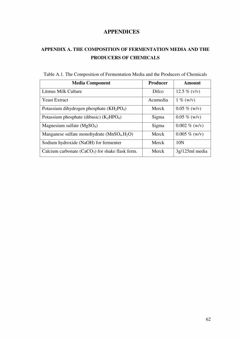
62
APPENDICES
APPENDIX A. THE COMPOSITION OF FERMENTATION MEDIA AND THE
PRODUCERS OF CHEMICALS
Table A.1. The Composition of Fermentation Media and the Producers of Chemicals
Media Component Producer Amount
Litmus Milk Culture Difco 12.5 % (v/v)
Yeast Extract Acumedia 1 % (w/v)
Potassium dihydrogen phosphate (KH2PO4) Merck 0.05 % (w/v)
Potassium phosphate (dibasic) (K2HPO4) Sigma 0.05 % (w/v)
Magnesium sulfate (MgSO4) Sigma 0.002 % (w/v)
Manganese sulfate monohydrate (MnSO4.H2O) Merck 0.005 % (w/v)
Sodium hydroxide (NaOH) for fermenter Merck 10N
Calcium carbonate (CaCO3) for shake flask ferm. Merck 3g/125ml media
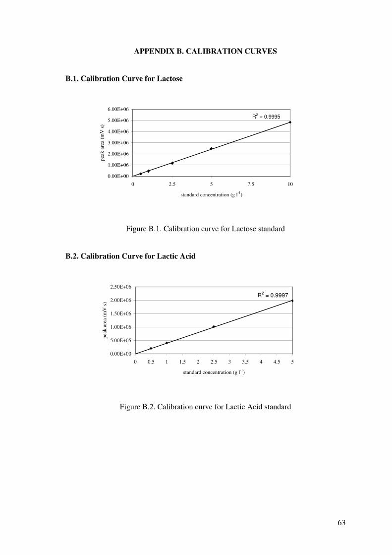
63
APPENDIX B. CALIBRATION CURVES
B.1. Calibration Curve for Lactose
R2 = 0.9995
0.00E+00
1.00E+06
2.00E+06
3.00E+06
4.00E+06
5.00E+06
6.00E+06
0 2.5 5 7.5 10
standard concentration (g l-1)
peak
are
a (m
V s
)
Figure B.1. Calibration curve for Lactose standard
B.2. Calibration Curve for Lactic Acid
R2 = 0.9997
0.00E+00
5.00E+05
1.00E+06
1.50E+06
2.00E+06
2.50E+06
0 0.5 1 1.5 2 2.5 3 3.5 4 4.5 5
standard concentration (g l-1)
peak
are
a (m
V s
)
Figure B.2. Calibration curve for Lactic Acid standard
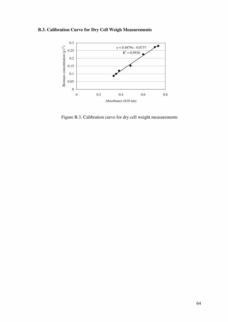
64
B.3. Calibration Curve for Dry Cell Weigh Measurements
y = 0.4879x - 0.0737R2 = 0.9938
0
0.05
0.1
0.15
0.2
0.25
0.3
0 0.2 0.4 0.6 0.8
Absorbance (610 nm)
Bio
mas
s co
ncen
trat
ion
(g l-1
)
Figure B.3. Calibration curve for dry cell weight measurements

65
APPENDIX C. LOWRY METHOD (TOTAL PROTEIN ASSAY)
C.1. Procedure
Reagents:
(a) 1 % CuSO4.5H2O.
(b) 1 % NaK tartrate.4H2O.
(c) 2 % Na2CO3 in 0.1 M NaOH.
(d) Commercial Folin-Ciocalteau reagent (sodium tungstate, sodium molybdate,
phosphoric acid, hydrochloric acid).
On the day of use, mix solutions (a) and (b) in a 1:1 ration and then dilute with
98 volumes of (c), to form the diluent. Dilute (d) 1:1 with distilled water to form the
color reagent.
Solutions (a), (b) and (c) are stable at room temperature for months. Solution (d)
is stable at 4 oC for months.
Method:
(i) Prepare a 0.2 ml sample (30-200 �g protein) in water.
(ii) Add 2.1 of diluent (alkaline copper reagent).
(iii) Allow to stand for 10 min.
(iv) Add 0.2 ml of color reagent and mix immediately.
(v) Allow to stand at room temperature (preferably in a dark place) for 1 h and read
the A550, against blank containing water and reagents. The color is stable (in the
dark) for several hours.
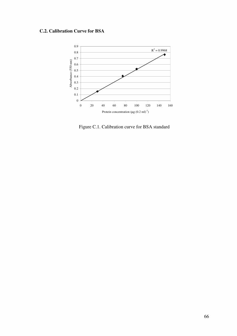
66
C.2. Calibration Curve for BSA
Figure C.1. Calibration curve for BSA standard
R2 = 0.9968
0
0.1
0.2
0.3
0.4
0.5
0.6
0.7
0.8
0.9
0 20 40 60 80 100 120 140 160
Protein concentration (µg (0.2 ml)-1)
Abs
orba
nce
(550
nm
)

67
APPENDIX D. THE RESULTS OF DIFFERENT MODELS FOR SAMPLE
FERMENTATION, 21.4 g l-1 INITIAL SUBSTRATE CONCENTRATION
D.1. Result of Model 1
Figure D.1. Model 1 and experimental data for 21.4 g l-1 initial substrate concentration;
experimental biomass concentration (+); experimental product formation (•); and
experimental substrate utilization (ο) and straight lines over them are model outputs
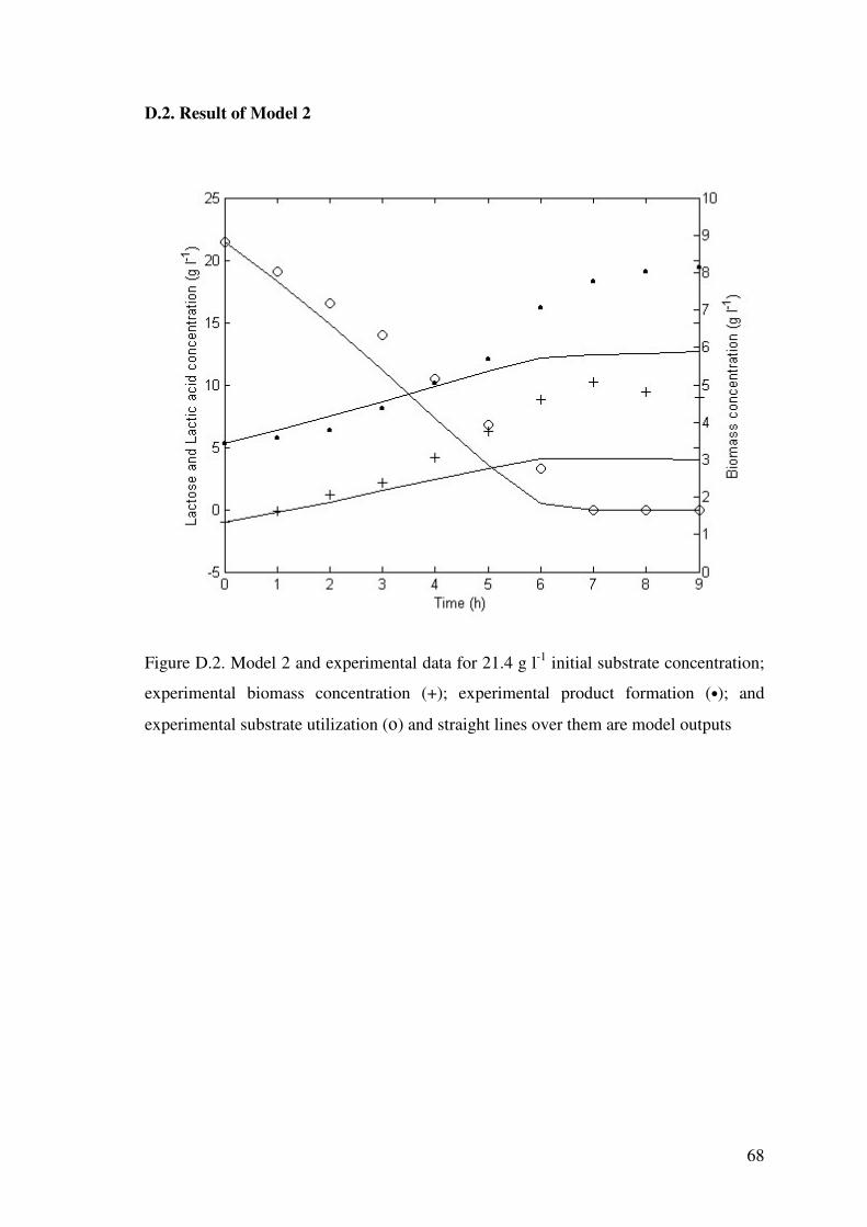
68
D.2. Result of Model 2
Figure D.2. Model 2 and experimental data for 21.4 g l-1 initial substrate concentration;
experimental biomass concentration (+); experimental product formation (•); and
experimental substrate utilization (ο) and straight lines over them are model outputs
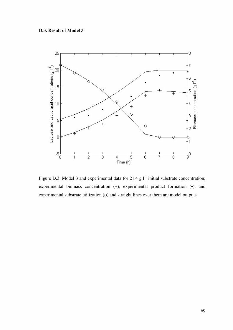
69
D.3. Result of Model 3
Figure D.3. Model 3 and experimental data for 21.4 g l-1 initial substrate concentration;
experimental biomass concentration (+); experimental product formation (•); and
experimental substrate utilization (ο) and straight lines over them are model outputs

70
D.4. Result of Model 4
Figure D.4. Model 4 and experimental data for 21.4 g l-1 initial substrate concentration;
experimental biomass concentration (+); experimental product formation (•); and
experimental substrate utilization (ο) and straight lines over them are model outputs
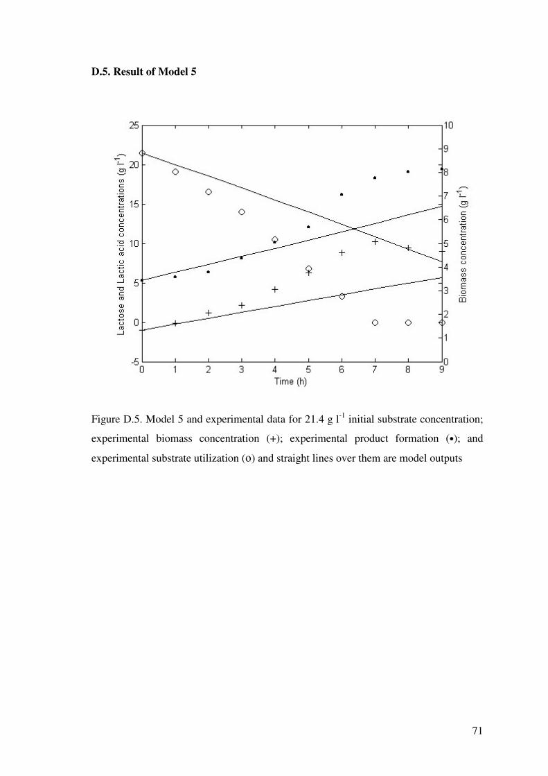
71
D.5. Result of Model 5
Figure D.5. Model 5 and experimental data for 21.4 g l-1 initial substrate concentration;
experimental biomass concentration (+); experimental product formation (•); and
experimental substrate utilization (ο) and straight lines over them are model outputs

72
D.6. Result of Model 6
Figure D.6. Model 6 and experimental data for 21.4 g l-1 initial substrate concentration;
experimental biomass concentration (+); experimental product formation (•); and
experimental substrate utilization (ο) and straight lines over them are model outputs
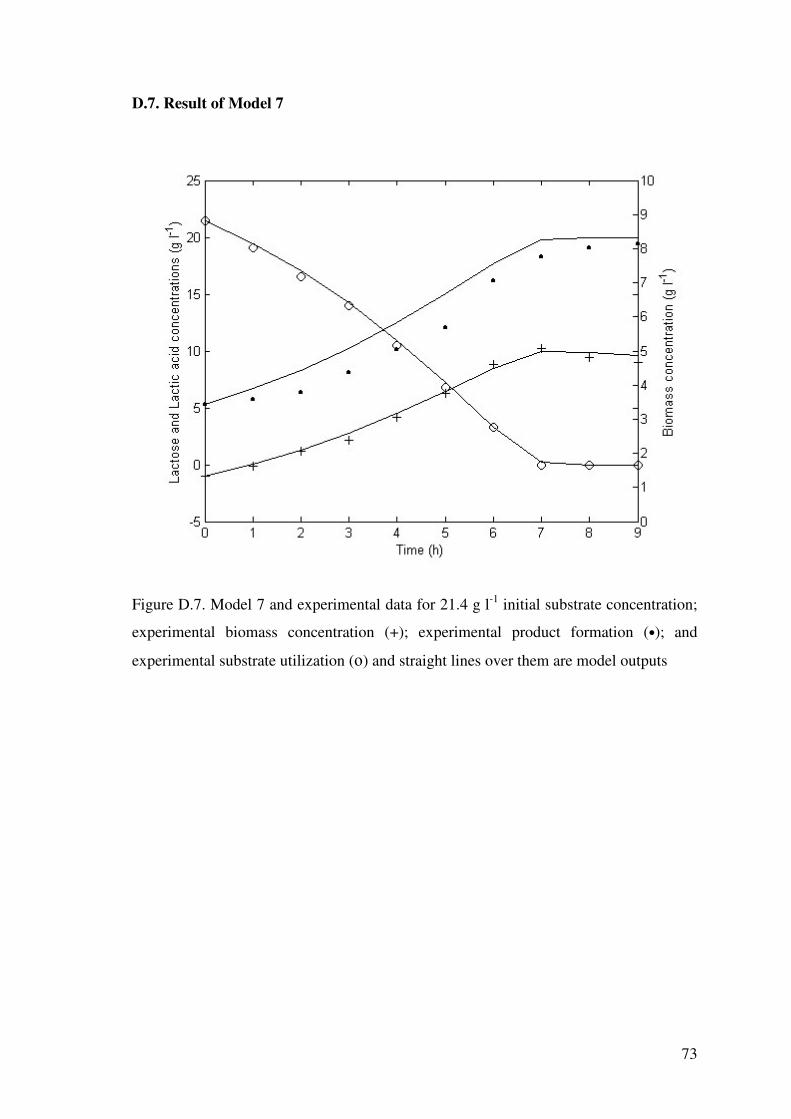
73
D.7. Result of Model 7
Figure D.7. Model 7 and experimental data for 21.4 g l-1 initial substrate concentration;
experimental biomass concentration (+); experimental product formation (•); and
experimental substrate utilization (ο) and straight lines over them are model outputs
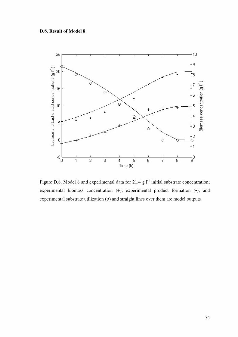
74
D.8. Result of Model 8
Figure D.8. Model 8 and experimental data for 21.4 g l-1 initial substrate concentration;
experimental biomass concentration (+); experimental product formation (•); and
experimental substrate utilization (ο) and straight lines over them are model outputs
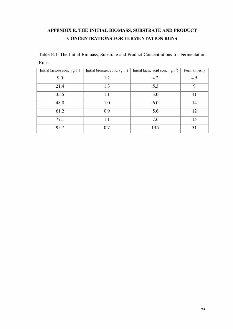
75
APPENDIX E. THE INITIAL BIOMASS, SUBSTRATE AND PRODUCT
CONCENTRATIONS FOR FERMENTATION RUNS
Table E.1. The Initial Biomass, Substrate and Product Concentrations for Fermentation
Runs Initial lactose conc. (g l-1) Initial biomass conc. (g l-1) Initial lactic acid conc. (g l-1) Ferm time(h)
9.0 1.2 4.2 4.5
21.4 1.3 5.3 9
35.5 1.1 3.0 11
48.0 1.0 6.0 14
61.2 0.9 5.6 12
77.1 1.1 7.6 15
95.7 0.7 13.7 31