kinetic models for wave propagation in random media

APAM Waves in Random MediaAPAM Waves in Random MediaAPAM Waves in Random Media

Kinetic models for wave propagation

in random media

Application to Time Reversal

Guillaume Bal

Department of Applied Physics & Applied Mathematics

Columbia University

http://www.columbia.edu/∼gb2030

[email protected]


Outline

1. Time Reversal in random media and kinetic models

2. Statistical stability and rigorous theories

3. Validity of Radiative Transfer Models

4. Applications to Detection and Imaging


Time Reversal framework

p

t

refoc

prefoc

t

Wave Solver+

Truncation

Wave Solver

Refocusing (?) Time

Reversal

p (0,x)χΩ(x)

p (T,x)t

χΩ(x)

− χ

χΩ

Ω

(x)

(x)t

(0,x)

(0,x) p (T,x)

p (T,x)

p (T,x)

p (0,x)


Numerical Experiment: Initial Data


Numerical Experiment: Forward Solution


Numerical Experiment: Truncated Solution


Numerics: Time-reversed Solution


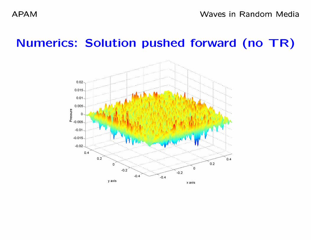
Numerics: Solution pushed forward (no TR)


Zoom on Refocused and Original Signals

−0.03−0.02

−0.010

0.010.02

0.03

−0.03−0.02

−0.010

0.010.02

0.03

−0.02

0

0.02

0.04

0.06

0.08

x axis

Zoom on the Refocused Signal

y axis

pres

sure

−0.03−0.02

−0.010

0.010.02

0.03

−0.03−0.02

−0.010

0.010.02

0.03

0

0.2

0.4

0.6

0.8

1

x axis

Zoom on the Initial Condition

y axis

pres

sure


Time-reversal in changing 3D media

We consider time reversal with possibly a change of media between the

forward (ϕ = 1) and backward (ϕ = 2) stages. The forward problem for

uϕ = (v, p) = (v1, v2, v3, p) is

Aϕ(x)∂uϕ(t,x)

∂t+Dj∂u

ϕ(t,x)

∂xj= 0, x ∈ R3, ϕ = 1,2,

with initial condition u1(t = 0) = u0; Aϕ(x) = Diag(ρ, ρ, ρ, κϕ(x)).

Using Green’s propagators Gϕ(t,x;y), the back-propagated signal is

uB(x) =∫R9

ΓG2(T,x;y)ΓG1(T,y′; z)χΩ(y)χΩ(y′)f(y − y′)u0(z)dydy′dz.

•Γ = Diag(−1,−1,−1,1) models the time reversal process

•χΩ(y) models the array of detectors and f(y) blurring at the detectors

•T is the duration of each propagation stages.


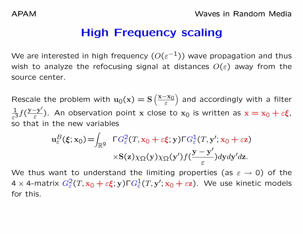
High Frequency scaling

We are interested in high frequency (O(ε−1)) wave propagation and thus

wish to analyze the refocusing signal at distances O(ε) away from the

source center.

Rescale the problem with u0(x) = S(x−x0ε

)and accordingly with a filter

1ε3f(y−y′

ε ). An observation point x close to x0 is written as x = x0 + εξ,

so that in the new variables

uBε (ξ;x0)=∫R9

ΓG2ε(T,x0 + εξ;y)ΓG1

ε(T,y′;x0 + εz)

×S(z)χΩ(y)χΩ(y′)f(y − y′

ε)dydy′dz.

We thus want to understand the limiting properties (as ε → 0) of the

4 × 4-matrix G2ε(T,x0 + εξ;y)ΓG1

ε(T,y′;x0 + εz). We use kinetic models

for this.


An adjoint Green’s matrix

Recall that the Green function G1(t,x;y) solves the equation

A1∂G1(t,x;y)

∂t+Dj ∂

∂xj(G1(t,x;y)) = 0, G1(0,x;y) = δ(x− y)I.

Introduce the adjoint Green’s matrix G1∗, solution of

∂G1∗(t,x;y)

∂t+∂G1

∗(t,x;y)

∂xjDj(A1)−1(x) = 0, G1

∗(0,x;y) = δ(x−y)ΓA−1(y)Γ.

We verify the following Maxwell reciprocity-type result

ΓG1(t,y;x) = G1∗(t,x;y)A1(x)Γ.

This allows us to recast the back-propagated signal as

uBε (ξ;x0)=∫R9

ΓG2ε(T,x0 + εξ;y)G1

ε∗(T,x0 + εz;y′)A1ε(x0 + εz)Γ

×S(z)χΩ(y)χΩ(y′)f(y − y′

ε)dydy′dz.


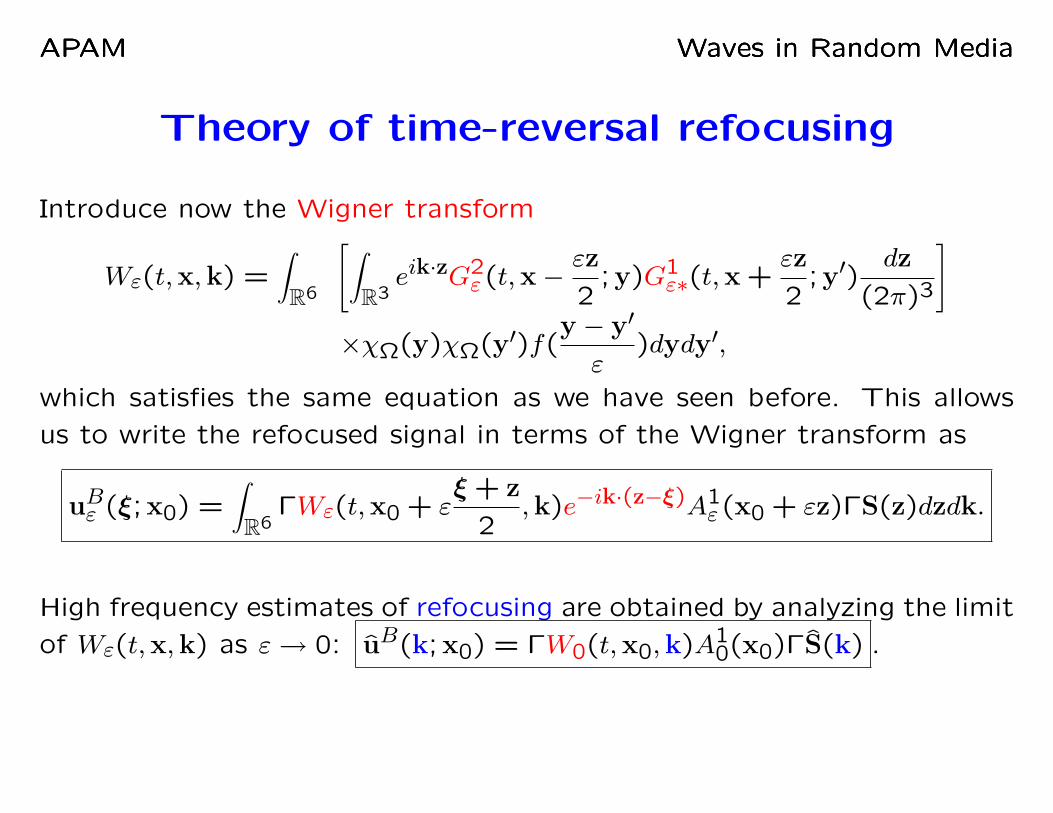
Theory of time-reversal refocusing

Introduce now the Wigner transform

Wε(t,x,k) =∫R6

[∫R3eik·zG2

ε(t,x−εz

2;y)G1

ε∗(t,x +εz

2;y′)

dz

(2π)3

]

×χΩ(y)χΩ(y′)f(y − y′

ε)dydy′,

which satisfies the same equation as we have seen before. This allows

us to write the refocused signal in terms of the Wigner transform as

uBε (ξ;x0) =∫R6

ΓWε(t,x0 + εξ + z

2,k)e−ik·(z−ξ)A1

ε(x0 + εz)ΓS(z)dzdk.

High frequency estimates of refocusing are obtained by analyzing the limit

of Wε(t,x,k) as ε→ 0: uB(k;x0) = ΓW0(t,x0,k)A10(x0)ΓS(k) .


Primer on Wigner Transform

The Wigner transform of two vector fields is defined by:

Wε[u,v](x,k) =∫Rdeiy·ku(x− ε

y

2)v∗(x + ε

y

2)dy

(2π)d.

It is the inverse Fourier transform of the product:

Wε[u,v](x,k) = F−1(u(x + ε

y

2)v∗(x− ε

y

2)).

We verify that ∫RdW [u,v](x,k)dk = (uv∗)(x)∫

RdkW [u,v](x,k)dk =

iε

2(u∇v∗ −∇uv∗)(x)∫

R2d|k|2W [u,v](x,k)dkdx = ε2

∫Rd∇u · ∇v∗dx.


Equations for the Wigner transform

Consider two field equations and the Wigner transform:

ε∂uϕε∂t

+Aϕεuϕε = 0, ϕ = 1,2, Wε(t,x,k) = W [u1

ε(t, ·),u2ε(t, ·)](x,k).

Then we verify that

ε∂Wε

∂t+W [A1

εu1ε ,u

2ε ] +W [u1

ε , A2εu

2ε ] = 0.

Calculations of the type

W [P (x, εD)u,v](x,k)=

∫R3d

eiy·ξeip·(x−y)P(ξ, ik + iε(p

2− ξ))W [u,v](y,k−

εξ

2)]dpdξdy

(2π)d

W [V (x,x

ε)u,v](x,k) =

∫R2d

eix·pε eix·qV (q,p)W [u,v](x,k−

p

2−εq

2)dpdq

(2π)2d,

allow us to obtain an explicit equation for Wε. The above formulas are

amenable to asymptotic expansions in ε.


Weak-Coupling Regime

In the weak coupling regime, the random fluctuations of the media are

modeled by

(cϕε )2(x) = c20 −√εV ϕ(

x

ε), ϕ = 1,2,

c20 =1

κ0ρ0, V ϕ(x) =

c20κ0κϕ1(x),

where c0 is the average background speed and κϕ1 and V ϕ are random

fluctuations in the compressibility and sound speed, respectively. We

assume that V ϕ(x), ϕ = 1,2, are statistically homogeneous mean-zero

random fields with correlation functions and power spectra given by:

c40Rϕψ(x) = 〈V ϕ(y)V ψ(y + x)〉, 1 ≤ ϕ,ψ ≤ 2,

(2π)dc40Rϕψ(p)δ(p + q) = 〈V ϕ(p)V ψ(q)〉.


Kinetic theory in weak coupling regime

The Wigner distribution at time t = 0 is given by

W (0,x,k) = |χΩ(x)|2f(k)A−10 (x), where (Aϕε )

−1 = A−10 +O(

√ε).

The limit Wigner distribution is decomposed as:

W (t,x,k) = a+(t,x,k)b+b∗++a−(t,x,k)b−b∗−. Furthermore, the radiative

transfer equation for a+ is (with ω+ = c0|k|)

∂a+∂t

+ c0k · ∇a+ + (Σ(k) + iΠ(k))a+

=πω2

+(k)

2(2π)d

∫RdR12(k− q)a+(q)δ

(ω+(q)− ω+(k)

)dq,

Σ(k) =πω2

+(k)

2(2π)d

∫RdR11 + R22

2(k− q)δ

(ω+(q)− ω+(k)

)dq

iΠ(k) =iπ∑j=±

4(2π)dp.v.

∫Rd

(R11 − R22

)(k− q)

ωj(k)ω+(q)

ωj(q)− ω+(k)dq.


Why is the refocusing stronger in

heterogeneous media ?

High frequency approximations of refocusing are given by

uB(k;x0) = ΓW0(t,x0,k)A10(x0)ΓS(k) .

where W (t,x,k) = a+(t,x,k)b+b∗+ + a−(t,x,k)b−b∗−.

Thus, the smoother the filter, the less distorted the back-propagated

signal uB. W0(t,x0,k), which solves the radiative transfer equation, is all

the smoother that scattering (proportional to R12) is strong.

In homogeneous media, W0(t,x0,k) is very singular and the backpropa-

gated signal very distorted, leading to poor refocusing. When the two

media are strongly correlated (so that R12 is large), W0(t,x0,k) is smooth

and refocusing is enhanced.


Outline






Statistical stability in Time Reversal

There are few theoretical results in the weak coupling regime for the wave

equation and they are concerned with ensemble averages of the Wigner

transform, not its limiting law.

However such limiting laws are accessible for simplifed regimes of radia-

tive transfer, including paraxial approximations, Ito-Schrodinger approxi-

mations, and random Liouville equations.

Such limiting laws directly translate into results on the statistical stability

of the time reversed signals whether the underlying media change or not

between the two stages of the time reversal experiment.


Two models where stability can be proved

• Paraxial (a.k.a. Parabolic) Approximation. Here, we obtain a (quan-

tum) wave equation with mixing time dependent coefficients. For a

typical wavelength (width of initial pulse) of order ε 1, the fluctuations

are of the form√εV (

x

ε,z

ε).

• Random Liouville Equations. Here the high frequency limit of the wave

equation (Liouville equation) with random Hamiltonian is used to show

that the Wigner transform solves in the limit ε → 0 a Fokker-Planck

equation. For a typical wavelength of order ε 1, the fluctuations are

of the form√δ(ε)V (

x

δ(ε)), C| ln ε|−2/3+η δ(ε) → 0 as ε→ 0.


PART 2.1: PARAXIAL

APPROXIMATION


Analysis for the Paraxial Equation

The pressure field p(z,x, t) satisfies the scalar wave equation

1

c2(z,x)

∂2p

∂t2−∆p = 0. (1)

The parabolic approximation consists of

p(z,x, t) ≈∫Rei(−c0κt+κz)ψ(z,x, κ)c0dκ,

where ψ satisfies the Schrodinger equation

2iκ∂ψ

∂z(z,x, κ) + ∆xψ(z,x, κ) + κ2(n2(z,x)− 1)ψ(z,x, κ) = 0,

ψ(z = 0,x, κ) = ψ0(x, κ)

with ∆x the transverse Laplacian in the variable x. The refraction index

n(z,x) = c0/c(z,x), and c0 is a reference speed.


Cartoon of Paraxial Approximation

x

z

L

a

MIRRORSOURCE

TIME-REVERSAL


Time Reversal within Paraxial Approximation

The back-propagated signal can be written as

ψB(x, κ)

=∫R3d

G∗(L,x, κ;η)G(L,y, κ;y′)χ(η)χ(y)f(η − y)ψ0(y′, κ)dydy′dη.

After introduction of the Wigner Transform and scaling, we get

ψBε (ξ, κ;x0) =∫R2d

eik·(ξ−y)Wε(L,x0 + εy + ξ

2,k, κ)ψ0(y, κ)

dydk

(2π)d.

The above formula shows that the asymptotic behavior of ψBε (ξ, κ;x0) as

ε→ 0 is characterized by that of the Wigner transform Wε(L,x,k, κ).


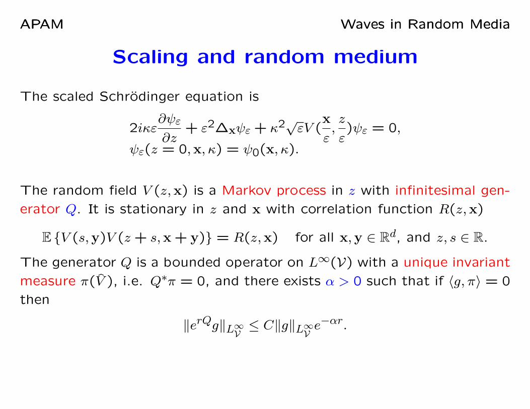
Scaling and random medium

The scaled Schrodinger equation is

2iκε∂ψε

∂z+ ε2∆xψε + κ2√εV (

x

ε,z

ε)ψε = 0,

ψε(z = 0,x, κ) = ψ0(x, κ).

The random field V (z,x) is a Markov process in z with infinitesimal gen-

erator Q. It is stationary in z and x with correlation function R(z,x)

E V (s,y)V (z + s,x + y) = R(z,x) for all x,y ∈ Rd, and z, s ∈ R.

The generator Q is a bounded operator on L∞(V) with a unique invariant

measure π(V ), i.e. Q∗π = 0, and there exists α > 0 such that if 〈g, π〉 = 0

then

‖erQg‖L∞V ≤ C‖g‖L∞V e−αr.


Equation for the Wigner Transform

∂Wε

∂z+

1

κk · ∇xWε = κLεWε

Wε(0,x,k;κ) = W0ε (x,k;κ),

LεWε =1

i√ε

∫Rd

dV (z

ε,p)

(2π)deip·x/ε

[Wε(x,k−

p

2)−Wε(x,k +

p

2)].

The initial condition is given by

W0ε (x,k;κ) =

∫Rdei(k+q)·y

(2π)dχ(x−

εy

2)χ(x +

εy

2)f(q)dydq.

It is uniformly bounded in L2(Rd×Rd) (hence so is Wε(z;κ)) and converges

as ε→ 0 to W0(x,k;κ) = |χ(x)|2f(k).


Main stability result

Let the array χ(y) and the filter f(y) be in L1∩L∞(Rd), while ψ0 ∈ L2(Rd)for a given κ ∈ R. The refraction index n(z,x) satisfies assumptions given

above. Then for each ξ ∈ Rd the back-propagated signal ψBε (ξ,x0, κ) con-

verges in probability and weakly in L2x0

(Rd) as ε→ 0 to the deterministic

ψB(ξ, κ;x0) =∫R2d

eik·(ξ−y)W (L,x0,k, κ)ψ0(y, κ)dydk

(2π)d.

The function W satisfies the transport equation

∂W

∂z+

1

κk · ∇xW = κLW,

with initial data W0(x,k) = f(k)|χ(x)|2 and operator L defined by

Lλ =∫Rd

dp

(2π)dR(|p|2 − |k|2

2,p− k)(λ(p)− λ(k)),

where R(ω,p) is the Fourier transform of the correlation function of V .


Result on the Wigner transform

Under the same assumptions, the Wigner distribution Wε converges in

probability and weakly in L2(R2d) to the solution W of the above transport

equation. More precisely, for any test function λ ∈ L2(R2d) the process

〈Wε(z), λ〉 converges to 〈W (z), λ〉 in probability as ε → 0, uniformly on

finite intervals 0 ≤ z ≤ L.

Here, 〈·, ·〉 is the usual scalar product in L2(R2d).


Details of the proofs

The scaling of the random fluctuations is supposed to be√εV (

x

ε,z

ε).

We then have the following equation for the scaled Wε:

∂Wε

∂z+ k · ∇xWε = LεWε

Wε(0,x,k) = W0ε (x,k),

with

LεWε =1

i√ε

∫Rd

dV (z

ε,p)

(2π)deip·x/ε

[Wε(x,k−

p

2)−Wε(x,k +

p

2)].

Thanks to the blurring at the detectors, we obtain uniform bounds in

L2 for the Wigner transform Wε independently of the realization of the

random medium.


Construction of approximate martingales

Let us define Pε as the probability measure on the space of paths C([0, L];X)

generated by Vε and Wε. Let λ(z,x,k) be a deterministic test function.

We use the Markovian property of the random field V (z,x) in z to con-

struct a first functional Gλ : C([0, L];X)→ C[0, L] by

Gλ[W ](z) = 〈W,λ〉(z)−∫ z0〈W,

∂λ

∂z+ k · ∇xλ+ Lλ〉(ζ)dζ

and show that it is an approximate Pε-martingale, more precisely∣∣∣EPε Gλ[W ](z)|Fs −Gλ[W ](s)∣∣∣ ≤ Cλ,L

√ε

uniformly for all W ∈ C([0, L];X) and 0 ≤ s < z ≤ L. Then there exists

a subsequence εj → 0 so that Pεj converges weakly to a measure P

supported on C([0, L];X). Weak convergence of Pε and the above error

estimate together imply that Gλ[W ](z) is a P -martingale so that

EP Gλ[W ](z)|Fs −Gλ[W ](s) = 0.

Taking s = 0 above we obtain the transport equation for W = EP W (z)in its weak formulation.

The second step is to show that for every test function λ(z,x,k) the new

functional

G2,λ[W ](z) = 〈W,λ〉2(z)− 2∫ z0〈W,λ〉(ζ)〈W,

∂λ

∂z+ k · ∇xλ+ Lλ〉(ζ)dζ

is also an approximate Pε-martingale. We then obtain that EPε〈W,λ〉2

→

〈W,λ〉2, which implies convergence in probability. It follows that the limit

measure P is unique and deterministic, and that the whole sequence Pε

converges.

That G2,λ[W ](z) is an approximate Pε-martingale uses very explicitly the

uniform a priori L2 bound on the Wigner distribution Wε.


PART 2.2: ITO SCHRODINGER

APPROXIMATION


Ito Schrodinger equations

Let us come back to the parabolic approximation

∂ψ

∂z+−iLz2kL2

x∆xψ =

ikLzν

2µ(Lxx

lx,Lzz

lz)ψ.

We now assume that the variations in z are very fast: lz λ. Then we

can formally replace

kLzν

2µ(Lxx

lx,Lzz

lz)dz by κB(

Lxx

lx, dz),

where B(x, dz) is the usual Wiener measure in z with statistics

〈B(x, z)B(y, z′)〉 = Q(y − x)z ∧ z′.


Ito Schrodinger equation

The parabolic equation in this regime becomes then

dψ(x, z) =iLz

2kL2x∆xψ(x, z)dz + iκψ(x, z) B(

Lxx

lx, dz).

Here means that the stochastic equation is understood in the Stratonovich

sense. In the Ito sense it becomes the Ito-Schrodinger equation:

dψ(x, z) =1

2

(iLz

kL2x∆x − κ2Q(0)

)ψ(x, z)dz + iκψ(x, z)B(

Lxx

lx, dz).

Advantage: Closed equations for the statistical moments.


First moment

The first moment defined by m1(x, z) = 〈ψ(x, z)〉 satisfies

∂m1

∂z(x, z) =

1

2

(iLz

kL2x∆x −Q(0)

)m1(x, z).

The L2 norm of the first moment

M2(z) =( ∫

Rd|m1(x, z)|2dx

)1/2.

is given by

M2(z) = e−Q(0)

2 zM2(0).

This shows that the coherent field m1 decays exponentially in z. This ex-

ponential decay is not related to intrinsic absorption. Instead it describes

the loss of coherence caused by multiple scattering.


Second Moment (I)

Energy propagation is better understood by looking at the second mo-

ment

m2(x1,x2, z) = 〈ψ(x1, z)ψ∗(x2, z)〉.

By application of the Ito formula we have

d(ψ(x1, z)ψ∗(x2, z)) = ψ(x1, z)dψ

∗(x2, z)+dψ(x1, z)ψ

∗(x2, z) + dψ(x1, z)dψ∗(x2, z).

This implies that

∂m2

∂z=

iLz

2kL2x(∆x1 −∆x2)m2 +

(Q

(Lx(x1 − x2)

lx

)−Q(0)

)m2.


Second Moment (II)

Introduce the rescaled variables: x =x1 + x2

2, y =

x1 − x2

η. Here the

adimensionalized wavelength ε η 1. Defining m2(x,y) = m2(x1,x2)

we have

∂m2

∂z=

iLz

kL2xη∇x · ∇ym2(z)−

(Q(0)−Q(y)

)m2(z).

Introduce the Wigner transform

W (x,p, z) =1

(2π)d

∫Rdeip·yψ(x−

ηy

2, z)ψ∗(x +

ηy

2, z)dy.

Then m2(x,y, z) =∫Rdeip·y〈W 〉(x,p, z)dp and

∂〈W 〉∂z

+Lz

kL2xη

p · ∇x〈W 〉 =∫Rd

[Q(p− p′)−Q(0)δ(p− p′)

]〈W 〉(p′)dp′.

We thus get an equation for the limiting Wigner transform for free.


Scintillation (moment of order 4)

We can similarly obtain an equation for the fourth moment:

m4(x1,x2,x3,x4, z) = 〈ψ(x1, z)ψ∗(x2, z)ψ(x3, z)ψ

∗(x4, z)〉.

We introduce the change of variables m4(x,y, z, t, z) = m4(x1,x2,x3,x4, z),

where x = x1+x22 , y = x1−x2

η , ξ = x3+x42 , t = x3−x4

η , η = lxLx. We obtain

∂m4

∂z=

iLz

kL2xη

(∇x · ∇y +∇ξ · ∇t)m4(z)−Qm4(z),

Q(x,y, ξ, t) =(2Q(0)−Q(y)−Q(t) +

∑εi,εj=±

εiεjQ(x− ξ

η+ εiy − εjt)

).


Scintillation = second moment for the WT

Define W(x,p, ξ,q, z) = W (x,p, z)W (ξ,q, z).

Its statistical average can be related to m4 and we find that

∂〈W〉∂z

+Lz

kL2xη

(p · ∇x + q · ∇ξ)〈W〉 = R2〈W〉+K12〈W〉

K12W =∫RdQ(u)e

i(x−ξ)·uη

(W(p− u

2,q−u2) +W(p + u

2,q + u2)

−W(p− u2,q + u

2)−W(p + u2,q−

u2))du

K2W =∫R2d

[Q(p− p′)δ(q− q′) + Q(q− q′)δ(p− p′)

]W(p′,q′)dp′dq′

R2W = K2W − 2Q(0)W.

When the phase term cancels so that “|K12W| 1”, we obtain that

Jη(x,p, ξ,q, z) = 〈W(x,p, ξ,q, z)〉 − 〈W (x,p, z)〉〈W (ξ,q, z)〉 ,the scintillation function, is small. The energy is then statistically stable.


Smallness of the scintillation function

Theorem. Let us assume that Wη(x,p,0) is deterministic and such that∫R2d

|Wη(x,p,0)|2dxdp +∫Rd

supx|Wη(x,p,0)|2dp ≤ C,

where C is a constant independent of η. Assume also that the correlation

function Q(x) ∈ L1(Rd) ∩ L∞(Rd). Then

‖Jη‖2(z) ≤ Cηd/2,

uniformly in z on compact intervals.


Weak statistical stability

Theorem. Under the assumptions of the previous theorem and λ ∈L2(R2d), we obtain that⟨(

(Wη, λ)− (〈Wη〉, λ))2⟩

≤ Cηd/2‖λ‖22.

Also (Wη, λ) becomes deterministic in the limit of small values of η as

P

(∣∣∣(Wη, λ)− (〈Wη〉, λ)∣∣∣ ≥ α

)≤Cηd/2‖λ‖22

α2→ 0 as η → 0.

The Wigner transform Wη of the stochastic field ψη converges weakly

and in probability to the deterministic solution W (x,p, z) of a Radiative

Transfer Equation.


Application to Time Reversal

Theorem. Assume that the initial condition ψ0(y) ∈ L2(Rd), the filter

f(y) ∈ L1(Rd)∩L2(Rd), and the detector amplification χ(x) is sufficiently

smooth. Then ψBη (ξ;x0) converges weakly and in probability to the de-

terministic back-propagated signal

ψB(ξ;x0) =∫Rdeik·ξW (x0,k, L)ψ0(k)dk,

whereW (x0,k, L) is the solution of a RTE with initial conditions W (x,k,0) =

f(k)|χ(x)|2. Moreover introducing λ(ξ,x0) = λ(x0)µ(ξ) we have the fol-

lowing estimate⟨(ψBη − 〈ψBη 〉, λ)2

⟩≤ Cηd‖ψ0‖22‖λ‖

22 = Cηd‖ψ0‖22‖µ‖

22‖λ‖

22,

uniformly in L on compact intervals.

We do not have such an estimate for the parabolic approximation.


Scintillation may appear and not disappear

Theorem. Assume that Wη(x,p,0) = δ(x − x0)δ(p − p0) [not physical

in Time Reversal]. Then the scintillation function Jη is composed of a

singular term of the form (with Q = Q(0)):

δ(x− ξ)δ(p− q)(α(x,p, z)− e−2Qzα(x− zp,p,0)

)plus other contributions that are mutually singular with respect to this

term. Moreover the density α(x,p, z) solves the radiative transfer equa-

tion with initial condition a0(x,p) = δ(x− x0)δ(p− p0):

∂α

∂z+ p · ∇xα+ 2Qα =

∫RdQ(u)

(α(x,p +

u

2, z) + α(x,p−

u

2, z)

)du.

The total intensity of this scintillation is (1 − e−2Qz) (so it grows in z

though it vanishes at z = 0).

In this case Energy is NOT statistically stable.


PART 2.3: RANDOM LIOUVILLE

REGIME


Stability by Random Liouville

Let us come back to the full wave equation and introduce vε(t,x) =

A1/2ε (x)uε(t,x) that satisfies the symmetrized system

∂vε

∂t+A

−1/2ε (x)Dj ∂

∂xj

(A−1/2ε (x)vε(x)

)= 0.

Define Pε(x,k) = P0(x,k) + εP1(x), where

P0(x,k) = iA−1

2ε (x)DjA

−12

ε (x)kj = icε(x)kjDj

2P1(x) = A−1

2ε (x)Dj ∂

∂xj

(A−1

2ε (x)

)−

∂

∂xj

(A−1

2ε (x)

)DjA

−12

ε (x).

The Wigner transform Wε(t,x,k) satisfies the evolution equation

ε∂Wε

∂t+ LεWε = 0

Lεf(x,k) =∫ (

Pε(y,q)eiφf(z,p)− f(z,p)e−iφPε(y,q))dzdpdydq

(πε)2d,

φ(x, z,k,p,y,q) = 2ε((p− k) · y + (q− p) · x + (k− q) · z).


The Liouville equations

The self-adjoint matrix −iP0 has eigenvalues λ0 = 0 of multiplicity d− 1

and λε1,2(x,k) = ±cε(x)|k| and can be diagonalized as

−iP0(x,k) =2∑

q=0

λεq(x,k)Πq(x,k), where2∑

q=0

Πq(x,k) = I.

The Liouville approximation to the Wigner transform is given by

Uε(t,x,k) =∑quεq(t,x,k)Πq(k),

where the coefficients uεq solve the Liouville equation

∂uεq

∂t+∇kλ

εq · ∇xuεq −∇xλεq · ∇ku

εq = 0

uεq(0,x,k) = TrΠqW0(x,k)Πq

Here, the coefficients λεq depend on δ(ε) and W0 is chosen independent

of ε.


Approximation of Wε by Liouville equation

Theorem. Let ρε(x) = ρ0 +√δρ1(

x

δ) and κε(x) = κ0 +

√δκ1(

x

δ), with all

terms sufficiently smooth. Then we have

‖Wε(t,x,k)− Uε(t,x,k)‖2 ≤ Cε

δmexp(

Ct

δ3/2)‖W0‖H3 + ‖W0

ε −W0‖L2,

for some m independent of ε.

In other words, assuming that W0ε converges strongly to W0 and that

δ(ε) → 0 as ε → 0 with the constraint δ(ε) | ln ε|−2/3+η, then the

difference ‖Wε(t,x,k) − Uε(t,x,k)‖L2 → 0 uniformly on final intervals t ∈(0, T ).

The convergence is uniform in the realization of the random medium (the

statistics of ρ1 and κ1 have not been defined yet). So we safely replace

the analysis of Wε by that of Uε, the solution of a Liouville equation with

random coefficients.


Analysis of the random Liouville equation

The Liouville equation is of the form

∂uε

∂t+(c0 +

√δc1(

x

δ))k ·∇xuε −

|k|√δ∇xc1(

x

δ) ·∇kuε = 0,

uε(0,x,k) = u0(x,k).

Its solution is given by uε(t,x,k) = u0(X(t),K(t)), where

−dX

dt=(c0 +

√δc1(

X(t)

δ))K, X(0) = x,

−dK

dt= −

|K(t)|√δ

∇xc1(X(t)

δ), K(0) = k.


Decorrelation of nearby particles

Let us assume that two particles satisfy the system for j = 1,2,

dX(δ)j (t)

dt =(c0 +

√δc1(

X(δ)j (t)

δ ))K(δ)j (t), X(δ)

j (0) = xj

dK(δ)j (t)

dt = 1√δ∇xc1(

X(δ)j (t)

δ )|K(δ)j (t)|, K(δ)

j (0) = kj.

Under suitable mixing conditions for c1 and for k1 6= k2, the laws of the

processes (K(δ)1 ,X(δ)

1 ,K(δ)2 ,X(δ)

2 ) converge weakly as δ → 0 to the law of

(K1,X1,K2,X2), where Xj(t) = xj + c0t∫0

Kj(s)ds, j = 1,2, and where

kj(·), j = 1,2 are independent symmetric diffusions in Rd \ 0 starting

at kj, j = 1,2 correspondingly with common generator

LF (k) =d∑

p,q=1

|k|2Dp,q(k)∂2kp,kqF (k) +

d∑p=1

|k|Ep(k)∂kpF (k).


Stability of the Wigner Transform

We deduce from the previous result that

Euε(t,x,k) → F (t,x,k) weakly as δ(ε) → 0,

where F satisfies the following Fokker-Planck equation

∂F

∂t+ c0k ·∇xF − LF = 0.

Moreover, we obtain the stability result

E∫ ∣∣∣⟨uε(T,x0,k)− F (T,x0,k), λ(k)

⟩∣∣∣2dx0

→ 0 as δ(ε) → 0,

which implies that uε converges in probability to the deterministic solution

F . This in turn implies the stability of the refocused signal uB.


Summary of radiative transfer models

We have obtained several transport models of the form

∂a

∂t+ c0k ·∇xa+ Sa = 0,

where the scattering operator S is given respectively by

Radiative Transfer: Sa =∫RdR(p− k)(a(k)− a(p))δ

(c0|p| − c0|k|

)dk

Paraxial: Sa =∫Rd−1

R(|p′|2 − |k′|2

2,p′ − k′)(a(k′)− a(p′))dk′

Ito-Schrodinger: Sa =∫Rd−1

R(0,p′ − k′)(a(k′)− a(p′))dk′

Fokker-Planck: Sa = −D(|k|)∆ka.

Note that Radiative Transfer and Fokker-Planck admit a diffusion limit

for small mean free paths. This can be arranged for the paraxial approx-

imation when R(t, ·) ≈ δ(t)R′(·), but not for Ito-Schrodinger.


Summary of Kinetic models for Time

Reversal

• We have a theory to express the high frequency limit of the refocused

signal in Time Reversal experiments using a Wigner transform. In the

scalar case, this expression is

uB(p;x0) = W (T,x0,p)S(p;x0).

The filter can also be generalized to changing environments.

• In certain cases, we can rigorously characterize the high frequency

limit of the Wigner transform and if possible (and true) obtain its sta-

bility. This has been done for the parabolic approximation and the Ito

Schrodinger approximation, and in the random Liouville regime, where

high frequency waves are approximated by particles propagating in ran-

dom media.


Outline






Time reversal in changing media

Consider two media with compressibility fluctuations given by κ2(x,k) =

φ(x)eiτ ·kκ1(x,k). For instance φ(x) corresponds to a change in the am-

plitude of the fluctuations at the macroscopic scale x and τ corresponds

to a spatial shift in the domain before back-propagation.

In the diffusive regime, the back-propagated signal takes the form

uB(k;x0) =

sin(ΠsT )

√κ0

ρik

cos(ΠsT )

p0(k) +

cos(ΠsT )ik

− sin(ΠsT )

√ρ

κ0

|k|ϕ(k)

× e−iτ ·k

sin |τ ||k||τ ||k|

e−Σψ2T/2 a(T,x0, |k|).

This is to be compared to the case where Πs = ψ = |τ | = 0 when the

medium remains the same during the forward and backward propagations.


2D Numerical simulations

In two space dimensions and in the case of periodic media with large

distances of propagation relative to the size of the box, the filter is

asymptotically given by

F (ψ, |τ |, |k|, T, L, kmax, κ) = a J0(|τ ||k|) cos(2ψΠ0T ) e−Σ2ψ

2T .

It should be compared to the numerical simulation

Fdata =(pB(x + τ), p0(x))

‖p0(x)‖2.

We consider some simulations with varying |τ | (shifting medium).


2D Numerical simulations (II)

Comparison of Fdata (solid lines) and the theoretical prediction F (dashed

lines) as a function of τ with ψ = 0. Periodic box of size L = 20,

propagation time T = 200, number of modes in power spectrum: 50.


Duke experimental setting


Spatial shift before backpropagation


Back-propagated signal

Back-propgated signal as a function of spatial shift for several frequencies.

The minimum of the back-propagated signal exactly occurs where it is

predicted by the two-dimensional theory.


Numerical validation of radiative transfer

Wave propagation in heterogeneous media may sometimes be difficult to

control in real experiments. Numerical simulations offer an interesting

complement to physical experiments.

In order to be relevant the simulations need to consider spatial domains

that are much larger than the typical wavelength in the system. This

requires us to use multi-processor architectures and parallelized codes.

We have developed such a computational tool to solve acoustic waves

(easily extendible to micro-waves) in the time domain.


Details of the wave (microscopic) code.The codes solves a discrete version (centered second-order discretization

in space and time) of the following acoustic wave system of equation

∂v

∂t+ ρ−1(x)∇p = 0,

∂p

∂t+ κ−1(x)∇ · v = 0.

The domain is surrounded by a perfectly matched layer (PML) method

so that outgoing waves are not reflected at the domain boundary. The

(random) physical coefficients ρ(x) and κ(x) are carefully chosen to verify

prescribed statistical properties.

The FDFT (Finite difference forward in time) method has been paral-

lelized by using the software PETSc developed at Argonne. Forward

calculations for T = 1500 (typical times necessary to validate the diffu-

sive model; for λ = 1 and average sound speed c0 = 1) require 3-4 days

of calculations.


Details of the macroscopic codes.

In both the direct and time reversal measurements, the data are the

macroscopic energy densities

E(t,x) =1

2

(ρ(x)|v|2(t,x) + κ(x)p2(t,x)

).

We consider two macroscopic models for E: a radiative transfer equation

and a diffusion equation. The radiative transfer equation is solved by a

Monte Carlo method (requiring in excess of 50M particles to achieve a

reasonable accuracy even with good variance reduction technique con-

ditioning particles on hitting the inclusion). The diffusion equation is

solved by the finite element method.


A typical configuration for the wave solver

R=50,40,30,20,10

300

PML

L

P PML

600

PML

M

Source(150,150)

Detector

150

Inclusion (450,150)

75

medium fluctuations 5−8%20 points per wavelengthλ=1

The domain size is roughly 20,000× 10,000 = 200M nodes


Wave-Transport-diffusion comparison

Experiment with isotropic

scattering (R ≡ 1 for this fre-

quency; the source term is

a localized Bessel function).

The best transport fit is ob-

tained for Σ−1num = 88.5 versus

Σ−1th = 83.00. The best fit for

the diffusion coefficient and

the extrapolation length are

Dnum = 43.2 and Lex = 0.80

versus Dth = (2Σ)−1 = 41.5

and Lth = 0.81.

Averaged energy densities on detector as a function of time.


Effect of void inclusion

Correction (w.r.t. solution without inclusion) generated by a void inclu-

sion, where the random fluctuations are suppressed. Left, radius of 40.

Right, radius of 50. Transport and diffusion generated by best energy

fit. The diffusion fit is valid only for very long times, whereas transport

performs extremely well.


Effect of increased randomness

Correction generated by an inclusion of radius R = 50 where the random

fluctuations are suppressed. Left: 5% RMS. Right: 8% RMS. Transport

and diffusion generated by best energy fit. The diffusion fit is now much

more accurate.


Effect of perfectly reflecting inclusion

Correction generated by a perfectly reflecting inclusion (specular reflec-

tion for transport and Neumann conditions for diffusion). Left, radius of

30. Right, radius of 40. Transport and diffusion generated by best energy

fit. Still very good agreement between wave and transport simulations.


Effect of a (4 times) smaller detector

0 1000 2000 3000

0

2

4

6

8

10

x 10−5

Time

Det

ecto

r Cor

rect

ion

Corrections, R=40, small detector

Wavetransport Σ−1=88.5

0 1000 2000 3000−2

−1

0x 10−4 Corrections, R=30, small detector

TimeD

etec

tor C

orre

ctio

n


Comparison of wave and transport predictions. Isotropic medium with

5% RMS. Left: void inclusion with R = 40; Right: reflecting inclusion

with R = 30.


Effect of a smaller inclusion

1000 2000 30000

2

4

6

8

10

x 10−5

Time

Corrections, R=20, isotropic case

Det

ecto

r Cor

rect

ion Wave

transport Σ−1=88.5

0 1000 2000 3000

−2

−1

0x 10−4 Corrections, R=10, isotropic case

Det

ecto

r Cor

rect

ion

Time


Comparison of wave and transport predictions with large detector. Isotropic

medium with 5% RMS. Left: void inclusion with R = 20; Right: reflect-

ing inclusion with R = 10. Conclusion: Radiative transfer is statistically

stable when sufficient averaging takes place.


Outline






Experimental setting; forward stage


Experimental setting; backward stage


Modeling the inclusion

The detection and imaging of buried inclusions (which are large com-

pared to the wavelength) is done as follows. We model the inclusion as a

variation in the kinetic parameters of the radiative transfer equation that

models the wave energy density.

The objective is to reconstruct these kinetic parameters from wave energy

measurements at the boundary of a domain. This is severely ill-posed

problem (in the sense that the reconstruction amplifies noise drastically).

Because the inclusion is assumed to be of small volume (at the macro-

scopic scale), further assumptions are possible. We consider asymptotics

in the volume of the inclusion, which take the form

δa0(t,x,k) = −|B|∫ t0G(t− s,x,xb,k) (Qa0)(s,xb,k)ds+ l.o.t.,

where a0 is the unperturbed solution, G the transport Green’s function,

Q the scattering operator and |B| ∼ Rd the inclusion’s volume.


Reconstruction of the inclusion

Detection and imaging based on the above asymptotic expansions allow

us obtain the inclusion’s location and volume:

σn/a0 error on R (%) error on xb error on yb0.25% 12 9.0 3.50.5% 25 15 5.01% 33 30 10

Very accurate data are required to locate and estimate the inclusion.


TR in Changing media; forward stage


TR in changing media; backward stage


Imaging and changing mediaIn the diffusive regime, the perturbation caused by a void inclusion is

given approximately by

δuD(t,x) = dπD0Rd∫ t0∇xu0(t− s,xb) · ∇xbG(s,x,xb)ds.

Here d is dimension and G(s,x,xb) the background Green’s function.

When we have access to the measured wave field both in the presence

and in the absence of the inclusion, we can consider the correlation of

the two fields. In the diffusive regime, the corresponding perturbation is

given by

δu(t,x) = −4πR∫ t0u0(t− s,xb)G(s,x,xb)ds+ o(R), d = 3

δu(t,x) =2π

lnR

∫ t0u0(t− s,xb)G(s,x,xb)ds+ o(

1

| lnR|), d = 2.

Since O(R) O(R3) in d = 3 and O(| lnR|−1) O(R2) in d = 2, it is much

easier to detect and image in the presence of differential information.


Can time-reversal experiments help?

Direct energy and time reversal measurements are hampered by two types

of noise: background noise ne and model noise nm (characterizing the

accuracy of the diffusive model). Let U be the direct measurement

and F the TR filter measurement. Then we have that (after a few

simplifications)

δU = δU + nmU0 + ndδF = δF + nmF0 + εd/2nd; (d is dimension).

Thus both types of measurements are equally affected by the model noise.

However, because background noise does not refocus at the source loca-

tion, it is strongly attenuated in the TR experiment.

In practice, direct measurements are very faint and thus even very small

background noise renders the detection impossible. This is where time

reversal helps (and may justify its equipment cost).


References

• G.Bal, G. Papanicolaou and L.Ryzhik. Self-averaging in time reversal for the parabolic

wave equation. Stoch. Dyn., 2 (2002) 507–532

• G.Bal, T.Komorowski and L.Ryzhik, Self-averaging of Wigner transforms in random

media. Comm. Math. Phys., 242 (2003) 81–135

• G.Bal and L.Ryzhik, Time Reversal and Refocusing in Random Media, SIAM J. Appl.

Math. 63(5) (2003) 1475-1498

• G.Bal. On the self-averaging of wave energy in random media. Multiscale Model.

Simul., 2(3), (2004) 398-420, 2004

• G.Bal and R.Verastegui, Time Reversal in Changing Environment, Multiscale Model.

Simul., 2(4) (2004) 639-661

• G.Bal and O.Pinaud, Time Reversal Based Detection in Random Media, Inverse

Problems, 21(5) (2005) 1593-1620

• G.Bal and O.Pinaud, Accuracy of transport models for acoustic waves in random

media, submitted

kinetic models for wave propagation in random media

Documents