Kinetic Monte Carlo Simulation of Heteroepitaxial

Growth: Wetting Layers, Quantum Dots, Capping,

and NanoRings

T.P. Schulze∗and P. Smereka

†

September 21, 2012

Abstract

A new kinetic Monte Carlo algorithm that efficiently accounts for elastic strain is presentedand applied to study various phenomena that take place during heteroepitaxial growth. Forexample, it is demonstrated that faceted quantum dots occur via the layer-by-layer nucleationof pre-pyramids on top of a critical layer with faceting occurring by anisotropic surface diffusion.It is also shown that the dot growth is enhanced by the depletion of the critical layer whichleaves behind a wetting layer. Capping simulations provide insight into the mechanisms behinddot erosion and ring formation. The algorithm used for the simulations presented here is basedon the observation that adatom and dimer motion is essentially decoupled from the elasticfield. This is exploited by decomposing the film into two parts: the weakly bonded portion andthe strongly bonded portion. The weakly bonded portion is taken to evolve independent of theelastic field. In this way the elastic field need only be updated infrequently. Extensive validationreveals that there is little loss of fidelity but the algorithm is fifteen to twenty times faster.

1 Introduction

The simulation of heteroepitaxial growth using kinetic Monte Carlo (KMC) is a promising alter-native to continuum formulations such as island dynamics (e.g. Refs. [1, 2, 3]), phase field models(e.g. Refs. [4, 5]), or sharp interface models (e.g. Refs. [6, 7, 8, 9]). The potential benefit ofKMC lies in that it can naturally include both discrete and stochastic effects that occur at thenanoscale. Unfortunately, the computational cost incurred by the need to repeatedly update theelastic displacement field makes the use of KMC challenging. However, starting with the work ofLam, Lee, and Sander[10], it became clear that it could be practical to use KMC as a tool to simu-late strained epitaxial growth. Since then there have been a number of papers that have improvedthe state-of-the-art in this area (e.g. Refs. [11, 12, 13, 14, 15, 16]).

In this paper, we present an approach that offers significantly improved computation times forsimulating heteroepitaxial growth. Indeed, our simulations are fifteen to twenty times faster thanprevious ones. Importantly, this has allowed us to access physically relevant parameter regimes in

∗Department of Mathematics, University of Tennessee, Knoxville, TN 37996.†Department of Mathematics, University of Michigan, Ann Arbor, MI 48109.

1

three dimensions. The new approach takes advantage of a natural separation of length scales thatoccurs in strained heteroepitaxial growth. Specifically, we use a surface decomposition formulationin which the weakly bonded atoms (e.g. adatoms and dimers ) are decoupled from the rest of thefilm and the associated elastic fields. Before we describe the method further, we wish to emphasizeseveral physical issues the improved method has allowed us to explore.

1.1 Heteroepitaxial Phenomena

To begin, we revisit what is typically referred to as Stranski-Krastanov (SK) growth. This is thescenario normally encountered during strained heteroepitaxial growth, starting off as layer-by-layer,but then suddenly transitioning to island-mode growth after a number of monolayers have beendeposited. For example, when depositing InAs on GaAs it is observed that three dimensionaldots form after 1.5 ML of deposition [17]. This suggests some sort of instability has occurred;however, the issue is rather more complicated than that. The early work of Asaro & Tiller [18] andGrinfeld [19] reveals a critical thickness of zero—all strained films are unstable irrespective of theirthickness. This, in turn, lead Spencer, Voorhees and Davis [8] to suggest that the critical thicknessobserved in experiments is an “apparent critical thickness,” the suggestion being instability isthere at all thicknesses, but is not readily observed until it reaches a certain stage of development.An alternative explanation originated with the work of Tersoff [20]. Based on calculations usingintermolecular potentials, he argued that up to three layers of Ge would be stable on Si. This led tomodels with wetting potentials, e.g. Ref. [7], with a specified critical thicknesses “hard-wired” intothe form of the potential. More recently, Baskaran and Smereka [21], have used a 1+1 dimensionalKMC theory to show that there is indeed a critical thickness, but that subsequent growth of theislands actually leads to a depletion of the original critical layer, leaving behind what we will referto as a wetting layer.

Although kinetic Monte Carlo models in 1+1 dimensions (e.g. [10, 21, 22, 23, 24, 25]) offer muchinsight into strained epitaxial growth, they cannot be considered definitive, as there are significantdifferences between the behavior of atomistic models in 2+1 and 1+1 dimensions. For example,in equilibrium it is known that a one dimensional surface cannot have true facets, whereas twodimensional surfaces can form facets below the roughening temperature (e.g. [26], p. 60). Thisis also reflected by the fact that the equilibrium shape of an island for a bond counting model isconvex in two dimensions [27, 28] but not so in three dimensions [29]. Other differences betweentwo and three dimensions are discussed by Leamy, Gilmer, and Jackson [30]. These differences canbe hidden in the context of continuum models. For example, the Wulff shape can be arbitrarilyspecified to give facets irrespective of dimension.

With this discussion in mind, our first aim here is to closely examine the emergence of facetedislands—quantum dots. Again, this issue is especially confusing and cannot be completely un-derstood from a continuum perspective. The very existence of a wetting layer indicates that theinitial growth direction should be a facet, and it has been argued that it should be very difficultto change this growth direction. Often, continuum models have dealt with this issue by modifyingthe growth law to induce the growth of new facets. While this gives the correct growth shapes,it cannot offer a mechanism by which this happens. Our KMC simulations suggest, in agreementwith the prediction of Xiang et al. [31], that the mechanism is the layer-by-layer nucleation of apre-pyramid which then evolves into a fully faceted pyramid by anisotropic surface diffusion. By“pre-pryamid” we mean a small multilayer three dimensional island whose sides are not faceted.Pre-pryamids can be either circular or irregular in shape.

We next turn to the topic of capping of the quantum dots with additional layers of the substrate

2

material. Our KMC simulations show that the capping procedure can lead to significant erosionof the quantum dots, in agreement with experimental observations. In addition the simulationsreveal a possible mechanism for this erosion: it is energetically favorable for the wetting layer tobe composed of dot material, therefore as the capping proceeds dot material is driven from dotsonto the wetting layer by capillary-like forces. Our simulations can also reproduce a particularlystriking result: the act of capping can produce ring-shaped dots. This result seems to indicate thatring formation is the result of strain relaxation. Finally, our simulations provide some new insightinto the mechanisms that lead to the alignment of stacked quantum dots.

1.2 Computational Framework

Our method is based on the observation that adatoms and dimers are weakly coupled to the elasticfield. Several tests reveal that this is an excellent assumption which also sheds light on aspectsof heteroepitaxial growth. For example, our calculations show that the mechanism involved inthe stacking of quantum dots involves a collective phenomena and is not the result of enhancednucleation in the region above the buried dot.

To get at the issues outlined above, we needed to introduce further modifications to our earliermethods aimed at improving computational speed. Our goal is to perform simulations on lengthscales close to one hundred nanometers and time scales of tens of seconds in physically realisticparameter regimes. Unfortunately, simulating epitaxial systems with strain is orders of magnitudemore expensive than simulating systems without strain because the elastic displacement field isnonlocal and often sensitive to atomistic scale detail. As a result, the bulk of KMC simulations ofheteroepitaxial growth have implemented some form of elastic update after each atomistic event.Much of the recent effort in this area has focussed on efficient algorithms for computing thisdisplacement field using a combination of both local and global updates [13, 14, 15, 16, 22]. Evenwith the techniques and approximations introduced in these earlier works, it would take somethingon the order of a year to complete the sort of computations we are striving for. To achieve ourgoals, the current simulations exploit a separation of scales based on the local coordination ofsurface atoms. More specifically, the surface of the film is partitioned into two nonoverlappingregions, S = Sw ∪ Ss, according to how strongly individual atoms are bonded to the surface.

Following the work of Burton, Cabrerra and Frank (BCF) [32], there has been a long traditionin the epitaxial growth literature of partitioning the film surface into a height profile, h(x), and an“adatom” density, ρ(x), of uncoordinated surface atoms. This recognizes the fact that, to a goodapproximation, these atoms diffuse independently on the surface of the film. This idea has beenextended to heteroepitaxial growth, and used to perform simulations using the island dynamicsformulation of a BCF-like model [1, 2, 3]. The approximation we have in mind is inspired by thesesimulations. A key observation made by these investigators is that it should not really be necessaryto update the elastic displacement field based on the motion of individual adatoms. In the caseof island dynamics, this observation is very naturally incorporated since an implicit time steppingstrategy is employed when updating the adatom field. In this way, many adatoms will attach ordetach from the island boundary before the elastic field is updated.

Within the KMC literature, which aims for a more resolved atomistic view of the film surface,the adatom concept has also occasionally found uses, as the motion of adatoms invariably dominatesthe computational cost of KMC simulations. In Ref. [33], for example, the surface of the film ispartitioned into regions surrounding steps, where KMC simulations are performed, and “vicinal”regions, where diffusion equations conserve the flux of adatoms to the steps. Adatom motion istreated using a “big-hop” approximation in Ref. [28]. More recently, in Ref. [16] it was observed

3

that the influence of the elastic field on the rates of adatoms was relatively weak, and that adatomshad a correspondingly weak influence on the elastic field of neighboring sites. Thus, omittingthe elastic computations for adatom motion is both highly efficient, due to the dominance ofthese events, and reasonably accurate. This latter study again relied on a version of the big-hopapproximation that, while effective, proved somewhat difficult to implement. Here, we adopt analternative approach, based on the domain decomposition mentioned above, that offers both astreamlined implementation and is readily extended to include any sort of weakly bonded atom.The result is surprisingly effective, yielding simulations that are fifteen to twenty times faster whileretaining a high degree of accuracy.

In the next section, we review the model and previous numerical approximations of this modelbefore continuing with the present approach.

2 KMC Model

Like most KMC models, we assume a Markov chain dynamics that has the system making transi-tions between states that consist of nearest neighbor single-atom moves on the surface.

2.1 General Considerations

In an off-lattice KMC, based on transition state theory and an empirical potential or perhaps evena density functional theory, one would compute hopping rates between states w and w′ as

rw→w′ = K exp [−EB/kT ],

where k is Boltzmann’s constant, T is the temperature of the film, and 1/K is a time scale deter-mined by details of the crystal, typically K = 1012 to 1013 sec−1, and EB = ET −EW is the energyneeded to rise out of a local minimum of the potential with energy EW , cross a transition/saddlepoint with energy ET , and escape to a neighboring local energy well. It is easy to show that thesemodels satisfy detailed balance.

In a lattice-based model without elastic effects, the energy is only defined for lattice configura-tions, and the energy barrier EB is often taken to be linear in the number and types of bonds toadjacent lattice sites. If one defines an Ising model potential,

U = −Nε,

based on a similar bond-counting scheme with N the total number of bonds in the system and ε abond energy, then one can see that such bond-counting models for the rates are equivalent to thefollowing:

EB = −∆U, where

∆U = U(with surface atom (i, j))− U(without surface atom (i, j)). (1)

In equilibrium, the probability of being in state w is

ρw = C exp(−U(w)/kT ),

where C is a normalization constant. Detailed balance requires

rw→w′ρw = rw′→wρw′ .

4

The bond-counting model for the rates in the form (1) is readily seen to satisfy this relationship.Notice that the term U(without surface atom(i, j)) is playing the role of the transition-state energy.It is important that this quantity is the same between any pair of communicating states. By definingthe “transition state” in this way, this condition is automatically satisfied, as the “atom off” stateis the same for both the original configuration and the destination regardless of which way thetransition takes place.

In reality −∆U is a fairly poor approximation to EB . To gain additional flexibility in the modelwithout altering the detailed balance relationship, we can modify this to EB = −(U0 +∆U). Thisis the most commonly used model in the KMC literature.

The type of model that we consider in this paper was proposed by Orr et al. [25] and has beenextended by a number of different investigators (e.g. [10, 12, 14, 15, 22]). In short, this is a cube-on-cube, bond counting model that has been modified to include elastic effects. The state of thesystem is described by a discrete height array hij , supplemented by a discrete displacement field,uijk. Associated with each of these is a potential energy—the former corresponding to an Isingtype potential U , the latter a discrete elastic energy W . We assume these quantities add to givethe total energy of the system E = U +W . This model is capable of capturing many qualitativeaspects of heterepitaxial growth. It is, however, still limited in that it uses a simple cubic latticeand cannot account for crystal defects, e.g. dislocations.

In a fashion similar to the bond-counting model (1), the transitions occur with rates that onlydepend on the initial state and the location of the hopping particle:

rij = K exp [(E0 +∆E)/kBT ], (2)

where {ij} indicates the initial position of the atom making the move and −(E0+∆E) is the energybarrier that must be overcome in making the transition. As with U0 above, we take E0 as a fixedconstant and

∆E = E(with surface atom (i, j))− E(without surface atom (i, j)). (3)

Like the energy, ∆E now consists of two pieces: one that depends only on hij and that is of the typefound in bond-counting schemes without elastic effects and one that depends only on the elasticenergy,

∆E = ∆U +∆W.

Finally, W is the total elastic contribution to the energy and, in analogy with (1), we have

∆W = W (with surface atom (i, j))−W (without surface atom (i, j)). (4)

The rates given by (2) also satisfy detail balance.

2.2 Model Parameters

As described in Ref. [16], we shall consider two species of atoms denoted type 1 and type 2. Formost of our simulations we will consider the situation in which atoms of type 2 are deposited on asubstrate of type 1. We will let γαβ denote the bond strength between atoms of type α and typeβ. For this model, ∆U for a surface atom at site (i, j) is given by

∆U = −(B11 +B22 +B12), (5)

withBαβ =

(aN

(1)αβ + bN

(2)αβ + cN

(3)αβ

)γαβ , (6)

5

where γαβ is strength of the interaction, N(1)α,β denotes the total number of bonds of type α and β

connecting the atom at site (i, j) and its nearest neighbors, N(2)αβ and N

(3)αβ are analogously defined

but for next nearest neighbors and next to next nearest neighbors respectively. We choose

E0 = −ED + (a+ 4b+ 4c)γ12.

This implies that ED is the energy barrier for the diffusion of a type 2 adatom on a type 1 substrate(ignoring the ∆W term for now). We point out that more sophisticated bond counting models havebeen proposed in Refs. [23, 24] in the context of heteroepitaxy.

The parameters a, b, and c allow one vary the anisotropy of the crystal. For example, thesurface energy per unit area for (100) facet of material 1 is

σ001 =(a+ 4b+ 4c)γ11

2ℓ2,

where ℓ is the size of the cubic unit cell. In addition the surface energy per unit area for the (011)and (111) facets are, respectively, given by

σ011 =(2a+ 6b+ 4c)γ11

2ℓ2√2

and

σ111 =(3a+ 6b+ 5c)γ11

2ℓ2√3

.

These expressions are computed by counting the number of broken bonds. The values σ001 andσ011 can be found in the book by Markov [34].

The elastic interactions are accounted for by using a ball and spring model with longitudinal anddiagonal springs having spring constants kL and kD respectively. The elastic effects arise becausethe natural bond length of materials 1 and 2 are different. We will denote these lengths as a1 anda2. The misfit is then µ = (a2 − a1)/a1. The details of this model can be found in Russo andSmereka [14] and Baskaran et al. [22]. For this model, if one has a flat film of material 2 on asubstrate of material 1 then the elastic energy per bulk atom in the film is

wfilm =4k2D + 5kLkD + k2L

kL + 2kDµ2.

The spring constants will be estimated by using the continuum limit of the ball and springmodel. For the single species case, the energy per atom can be written as

watom = (ℓ2/2)[(kL + 2kD)(e

211 + e222 + e233) + 2kD(e11e22 + e11e33 + e22e33) + 4kD(e

212 + e213 + e223)

],

where eij is the strain tensor. The energy density per unit volume is then w = watom/ℓ3. Thereforewe can write

w =1

2C11(e

211 + e222 + e233) + C12(e11e22 + e11e33 + e22e33) + 2C44(e

212 + e213 + e223),

whereC11 = (kL + 2kD)/ℓ, C12 = kD/ℓ, and C44 = kD/ℓ.

The above formulas will be used later in the paper.

6

3 KMC Implementation

In this section, we start by reviewing the Local Energy Method which was introduced in Ref.[16]. While this was a significant advance, allowing the computation of three-dimensional films onscales previously unreachable, we were unable to access physically realistic parameter regimes whichhave lower deposition rates and larger islands than we were able to compute with that method.In Section 3.2, we gain another leap in computational performance through the use of a surfacedecomposition technique, allowing us to access physically realistic regimes. The rest of the sectionis spent validating the method by comparing to the results of the previous method.

3.1 Local Energy Method

It is specifically the computation of ∆W that makes these simulations so much more costly thansimulations that involve only a bond-counting formula, as each rate requires one to solve a linearsystem, and, in principal, one needs to update the hopping rate of all of the surface atoms aftereach event. In Ref. [16], an approximation is introduced that goes a long way toward mitigatingthis problem. It is observed that ∆W is close to being proportional to the energy in the springsimmediately adjacent to the atom whose rate is being calculated; in other words

∆Wij = Cwij, (7)

where wij is the energy in the springs connected to the surface atom at site (i, j) and C dependsonly on the ratio of the spring constants kL and kD. For example, if kL = 2kD then C = 1.33 andif kD = (10/3)kL, C = 1.5 (see Figure 1 of Ref. [16] for the first case).

While this is not an exact relationship, arguments based on continuum elasticity suggest theerror is small, and careful comparison with simulations not using this approximation support thisassertion, which has the added advantage of being relatively easy to explain and implement, sowe will use this approach in all of the calculations presented in this paper. We refer to thisas the Local Energy Method. This approximation is similar to that used in Ref. [3]. For aprocedure somewhat more faithful to the model introduced above, an alternative would be to usethe techniques introduced in Ref. [15].

With this approximation in place, only a single linear system need be solved per event. Even thisis a large numerical task when compared to the local update that accompanies an event in a simple,bond-counting KMC simulation. Ultimately, we will deal with these calculations in one of threeways. Moves of low-coordinated atoms will use rates that depend only on the bond counting part, aswe will demonstrate that the elastic contribution is negligible. For the highly-coordinated atoms, wewill mostly rely on a locally constrained calculation, where the displacement field beyond a certaindistance from the move is held fixed and serves as a boundary condition for the local update. Wehave used these local updates in our earlier work, developing an efficient numerical procedure, theExpanding Box Method, to perform these calculations [15, 22]. Similar ideas have been used in off-lattice simulations [35, 36], where this is typically referred to as a “frozen crystal” approximation.The local calculations leave small residual forces at the boundaries, which accumulate over thecourse of the calculation, and must occasionally be relaxed by performing a full, global solution ofthe system. The latter calculations use an artificial far-field boundary condition with a multigridprocedure for solving the linear system [13, 14].

7

3.2 Surface Decomposition KMC

The new technique being introduced in this paper is to decompose the surface into two subsets,one for highly coordinated sites and one for low coordinated sites. Effectively, one has

hij = hij +∆hij ,

where hij is the profile of the film with the weakly bonded atoms removed. For the low-coordinatedsites, the bond-counting term, U , dominates, while both U and W (the elastic energy) are impor-tant for the highly-coordinates sites. This can be seen by examining Figures 1 and 2. Figure 1demonstrates how the variation in the elastic energy density is largely confined to the boundary ofislands and is not significantly affected by the removal of the adatoms and dimers from the surface.Figure 2 shows close-ups of the same calculations shown in Figure 1, but zoomed into the lowerleft quarter of the images in Figure 1. This view reveals important details, described below, of theelastic density field in the vicinity of adatoms and vacancies that are not readily apparent in thefirst view.

In the upper left panel of Figures 1 and 2, we have a typical surface configuration, showing twoquantum dots with many adatoms. The dots are resting on one monolayer of material 2 which,in turn, is on an infinitely deep substrate of material 1. It is important to note there are severalvacancies in the monolayer of material 2. In the panel below this, we plot the local elastic energy,wij : the total energy in the springs connected to the surface atom at site (i, j). One observes thatthis quantity is large around the rim of islands, where it would increase the hopping rate, and thatit is almost zero for both adatoms and vacancies that penetrate to the substrate. More carefulobservations reveal that not only is the local elastic energy of the adatoms small, but, unlike thevacancies, the adatoms do little to disturb their environment. This turns out to be true of all lowcoordinated sites, and is easy to understand in terms of the ball-and-spring model—there simplyis not much constraining a low-coordinated atom, so the springs can relax almost completely.

In the upper right panels of Figures 1 and 2, these low-coordinated atoms have been removedfrom the surface, and the resulting local elastic energy is plotted directly below in the lowerright panels. Notice that this has had little effect on the regions where the local elastic energyis large—the rims of the islands. Further, it replaces the local elastic energy at the locations wherelow-coordinated atoms have been removed with a local elastic energy that fits smoothly into itsenvironment. This is important because it means that these values can be used to get a realistichopping rate once the low-coordinated atom has moved off of the site without having to updatethe elastic field.

3.2.1 Detailed balance

The total energy of the system using the Surface Decomposition Method is approximated by

E = U +W,

where U is the bond-counting energy defined earlier and W is the elastic energy corresponding tothe profile h. When E is used in place of E in Eq. (2) the rates will still satisfy detailed balance,which can be seen as follows. As with the earlier model, the “atom off” state can readily be seen togive the same energy for any two states that are connected by an allowed transition, and this, onceagain, mimics the role of the transition-state energy, ensuring that detailed balance is satisfied.

8

3.2.2 Algorithm

1. Initialization

(a) Determine ∆U for every surface atom by bound counting.

(b) Determine the denuded configuration h by removing any surface atom with coordinationN ≤ NC = 6.

(c) Perform a global elastic solve for the configuration h, computing ∆W = Cwij for everysurface atom of the denuded configuration.

(d) The rates for surface atoms of the actual configuration h are then initialized to

rij =

{K ′ exp(∆U/kT ) if Nij ≤ Nc,K ′ exp(∆U/kT +∆W/kT ) if Nij > Nc,

where K ′ = KeE0/kT .

2. Select an event by choosing a uniformly distributed random number r ∈ [0, R), with R =rdep +

∑rij . The event to which r corresponds is located using a binary tree search [37].

3. If the event selected is a deposition, a site is selected at random and an atom is added there;otherwise the event is a hop and the selected atom is moved to one of the four lateral neighborsites selected at random.

4. The values of ∆Uij are updated as needed.

5. If the denuded configuration is changed then one performs a local elastic solve using anexpanding box of size S centered at the site of the selected atom.

6. Every NG = 105 steps, update the entire displacement field of the denuded configuration.The results are quite insensitive to the choice of NG; for example changing NG to 106 givessimilar results for all the cases presented in this paper.

7. Repeat steps 2 through 6.

3.3 Verification

It turns out that the new approach is fast enough that one can get much closer to simulatingphysically relevant systems. However, we wish to compare with our old approach in order toestablish the validity of the new formulation, which is now roughly fifteen times faster. Thiscomparison is not feasible using physically relevant parameters, so we choose more convenientparameters for this purpose.

Roughly speaking the surface energies are on the low side for semiconductor materials, whilethe spring constants are on the high side, but this allows us to observe island formation on timeand length scales accessible to our previous code.

In this section we take

a = 0.3, b = 0.5, c = 1, g11 = 0.26 eV, g12 = 0.2425 eV, and g22 = 0.225 eV.

9

0

20

40

60

80

100

120

140

0

20

40

60

80

100

120

140

0

0.1

0.2

0.3

0.4

0

20

40

60

80

100

120

140

0

20

40

60

80

100

120

140

0

0.1

0.2

0.3

0.4

Figure 1: The upper panels show surface configurations with and without low coordinated atoms,whereas the lower panels show the respective elastic energy densities. Notice that the elastic energyis low on the tops of the islands because the film is relaxed compared to the single monolayer ofcoverage on the rest of the surface. Also, notice that the largest concentration of energy density ison the boundary of the islands.

If one takes ℓ = 2.7 A, then for material 1 this corresponds to the following surface energies for theindictated facets:

σ100 = 1800 erg/cm2, σ110 = 1535 erg/cm2 and σ111 = 1468 erg/cm2.

In addition, we take µ = .05, kL = 15eV/ℓ2 and kD = 7.5eV/ℓ2, which corresponds to

C11 = 30eV/ℓ3 and C12 = C44 = 7.5eV/ℓ3,

orC11 = 24.42 × 1011 dynes/cm2 and C12 = C44 = 6.104 × 1011 dynes/cm2.

We take ED = 0.8, K = 1012, and T = 700 K.

10

510

1520

2530

3540

45

5

10

15

20

25

30

35

40

45

0

0.05

0.1

0.15

0.2

0.25

510

1520

2530

3540

45

5

10

15

20

25

30

35

40

45

0

0.05

0.1

0.15

0.2

0.25

Figure 2: This is the same as figure 1 except each panel is zoomed in to the lower right corner.This allows one to see individual adatom and vacancies. Notice that removal of adatoms has littleaffect on the surrounding energy density.

3.3.1 Submonolayer Growth

In our first test, we consider the deposition of 0.2 ML, at a rate of 0.5 ML/sec, of material 2 on asubstrate composed of material 1. The lattice is 512×512, which corresponds to roughly 138 nm ×138 nm. We compute the island size distribution for an ensemble with ten realizations using boththe Surface Decomposition Method and the Local Energy Method. The results are presented inFigure 3 and show good agreement. In addition, for further comparison, we present the island sizedistribution when elastic interactions are ignored. This shows that the effect of elastic interactions isto both narrow the size distribution and reduce the average size of the islands. This is in agreementwith the island dynamics simulation of Ratsch et al. [3].

11

5 10 15 200

50

100

150

200

250

300

effective radius

num

ber

dens

ity

Figure 3: Island size distributions for the Local Energy Method (in red), Surface DecompositionMethod (in blue), and with no elastic effects (in black). (color online)

0 10 20 30 40 50 60−5

0

5

10

15

R

g(R

)

Figure 4: The red and blue curves are the ensemble averaged auto correlation function for theSurface Decomposition Method and the Local Energy Method, respectively. Ten simulations wereused for each ensemble.

12

Figure 5: Three dimensional island formation after three monolayers of deposition computed usingboth the Local Energy Method and the Surface Decomposition Method. The qualitative similarityreinforces the detailed statistics presented in Figures 3 and 4.

20 40 60 80 100 120

10

20

30

20 40 60 80 100 120

10

20

30

Figure 6: Cross sections after 1.4 monolayers of deposition. The upper figure results from usingthe Local Energy Method, while the lower one uses the Surface Decomposition Method.

3.3.2 Three Dimensional Islands

Here we consider multilayer growth of material 2 on material 1 using a substrate of size 128× 128.The deposition rate is 1 ML/sec. In this simulation we see the formation of a wetting layer withsubsequent growth of three dimensional islands. Our basic tool for comparing results of differentsimulations is a radially averaged autocorrelation function. First, we define h = h− 〈h〉, where 〈h〉

13

0 0.25 0.5 0.75 1 1.25 1.50

1

2

3

4

5

6

7

8

monolayers

dot h

eigh

t

Figure 7: Dot height as a function of the number of deposited monolayers. The Surface Decom-position Method is plotted in blue, whereas the Local Energy Method is plotted in red. (coloronline)

Figure 8: Film profiles after 1.4 monolayers of deposition. The lefthand figure results from usingthe Local Energy Method, while the righthand figure uses the Surface Decomposition Method.

is the mean surface height and compute the discrete form of

I(u, v) =

∫ ∫h(x− u, y − v)h(x, y)dxdy,

followed by

g(R) =1

2πR

∫ ∫I (u(r, θ), v(r, θ)) δ(r −R)drdθ,

where one uses a suitably mollified delta function. This gives a fairly robust measure of filmcharacteristics at different length scales.

14

The results are summarized on Figure 4 which shows the ensemble average of 10 autocorrelationfunctions for each method. The figure shows that both methods produce autocorrelation functionsthat are in good agreement with each other. There is one slight difference, however. It seems thatthe Local Energy Method produces results that are slightly rougher than the Surface DecompositionMethod. Figure 5 shows two simulations after three monolayers of deposition, one with each of thetwo methods. The qualitative similarity of the two surfaces reflects the agreement seen in the datapresented in Figures 3 and 4.

3.3.3 Quantum Dot Alignment

In this test, we consider the situation in which a cylindrical region of material 2 is buried in thecenter of a substrate of material 1, henceforth referred to as a buried dot. For this test case, g12was changed to 0.23 to suppress the amount of intermixing. Material 2 is then deposited on to thesubstrate at a rate of 0.1 ML/sec. Due to the presence of the buried dot it is energetically preferredfor a three dimensional island to form directly above the buried dot. Indeed this is exactly whathappens. Figure 6 shows a cross section of our system after 1.4 ML of deposition. One can clearlysee the three dimensional island has aligned itself with the buried dot for both approaches. Toassess whether or not the dynamics of both approaches agree, we consider the following quantityreferred to as the dot height:

hdot =1

πR2

∫ ∫

|x−xc|<Rh(x, y)dxdy,

which is the average height in a local region centered over the buried dot. In the above formulax = (x, y)T and xc is the horizontal location of the center of the buried dot. Figure 7 shows a plotof the ensemble averaged island height as function of the amount of material deposited for bothmethods with R = 10. The agreement is quite good.

4 Applications and Implications

In this section we turn to the exploration of the issues outlined in Section 1.1.

4.1 Quantum Dot Alignment

The fact that this new, surface decomposition technique offers significant improvement in speedwhile at the same time preserving fidelity offers some insight into the importance of various physicalprocesses that take place during heteroepitaxial growth. In particular, it suggests that elasticinteractions play a very weak role for low coordinated atoms. This conclusion is significant whenone considers what happens during the alignment of stacked quantum dots. In has been suggestedin the literature (e.g. Ref. [38]) that adatoms move to the strained regions of the substrate that areover the buried dots, and, as a consequence, islands will nucleate in these regions. The results heresuggest something slightly different happens. Indeed, we observe that islands nucleate essentiallyat random without regard to the buried dot, and, only when they become big enough, do they startto interact elastically with the buried dots. Before that, the islands were small and dominated bysurface forces and entropy. This is demonstrated in Figure 9 which shows results for very smallamounts of deposition. For 0.02 ML of deposition, it is evident that the location of the small islandshas not yet been influenced by the buried dot. There does seem to be some slight bias at 0.05 MLand by 0.1 ML it is clear that the islands are finally big enough to interact significantly with theburied dot. The discussion above was developed, in part, from conversations with A. Baskaran.

15

Figure 9: Results after a very small amount of deposition. From left to right and top to bottomthe amount of material deposited is .02 ML, .05ML and .1 ML, respectively.

4.2 Parameter Values

Before we present our other series of simulations, we first discuss the issue of parameter values.We will consider a system where the parameters are somewhat close the physical properties of atypical semiconductor material. We are not claiming to simulate a particular system but instead asystem whose phenomena are representative of what happens in a variety of actual heteroepitaxialexperiments.

We again take a = 0.3, b = 0.5 and c = 1.0, but now we choose

g11 = 0.29 eV, g12 = 0.2599 eV, and g22 = 0.2510 eV.

If one takes ℓ = 2.7A then, for material 1, the surface energies for the following facets are

σ100 = 2007 erg/cm2, σ110 = 1712 erg/cm2 and σ111 = 1637 erg/cm2.

These numbers are somewhat close to the surface energies of Silicon. Notice that the surfaceenergies of the (100) interface for material 2 is about 13% smaller than material 1. These choicesare fairly close to those reported by Jaccodine [39]. The values for the (100) interface are also close

16

Figure 10: The film is shown after 0.5 monolayers of deposition of yellow colored atoms (Material 2)at T=750 K. At this stage in the growth only two dimensional islands have formed. The presenceof blue colored atoms within the two dimensional islands is due to intermixing.

to those chosen by Levine et al. [40]. In addition, the (110) and (111) facets have lower energythan the (100) facet, which is also true for Si and Ge.

We note that Mo et al. [41] report from experiments that the jumping rate of Si on Si(100)is well approximated by D/ℓ2 where D = 10−3 exp(−Ed/kT ) cm

2/sec and Ed ≈ 0.67 eV. Thisindicates that the hopping rate, assuming a lattice size of 2.7 A, is 1.37× 1012 exp(−Ed/kT ) sec

−1.In our simulations we take ED = 0.7 eV and choose the prefactor to be 1012. This means the energybarrier for the diffusion of an adatom of material 2 on material 1 is 0.7 eV while for material 1 onmaterial 1 it is 0.890 eV and for material 2 on material 2 is 0.640 eV. The diffusion barriers we arechoosing are still slightly too large and this is simply because the code is still somewhat slow. Forexample, the result shown in Figure 14 took approximately three weeks to generate. If we had usedmore realistic energy barriers for adatom hopping the simulations would have taken much longer.

For the elastic strengths we pick kL = 3 eV/ℓ2 and kD = 10 eV/ℓ2. In the continuum limit thisgives

C11 = 23 eV/ℓ3 and C12 = C44 = 10 eV/ℓ3.

Now taking ℓ = 2.7A we have

C11 = 18.73 × 1011 dynes/cm2 and C12 = C44 = 8.14× 1011 dynes/cm2.

These are not unreasonable values for a semiconductor. For example, at T = 0 the elastic constants

17

Figure 11: The film is shown after 1.0 monolayers of deposition at T=750 K. Here the two dimen-sional islands have grown into each other to completely cover the surface. While this single layerof yellow colored atoms is strained, the surface forces prevent the formation of three dimensionalislands.

of Silicon are

C11 = 16.4×1011 dynes/cm2, C12 = 5.92×1011 dynes/cm2, and C44 = 8.17×1011 dynes/cm2.

For the rest of our simulations we will take µ = 0.055. This value of the misfit is higher than onefor Si-Ge, but lower than for GaAs-InAs. We will take F = 1 ML/sec and, unless otherwise stated,T =750 K.

4.3 Stranski-Krastanov Growth

The results of our simulations using the Surface Decomposition Method are displayed in Figures10 to 14. These simulations shed light on the formation of faceted quantum dots on a facetedsurface, what Tersoff et al. [42] have refered to as a puzzling phenomenon. Since the quantumdots and the surface are fully faceted, they should be nucleated by a thermally activated process.One might think that the islands would be facetted as soon as they are nucleated, but experimentssuggest that instead the faceted quantum dots evolve from pre-pyramids. Recall that pre-prymidsare small, multilayer, three dimensional islands whose sides are not faceted.

Figure 10 shows the film after 0.5 ML of deposition, and demonstrates the formation of two-dimensional, i.e. single monolayer, islands. Figure 11 shows that, after 1.0 ML of deposition, the

18

Prepryamids

2D islands

A pyramid in an

early stage

of growth

✚✚

✚✚

✚❂

❄

✄✄✄✄✄✄✄✄✄✄✄✄✄✄✄✄✗

���������✒

❅❅❅❅❅❅❘

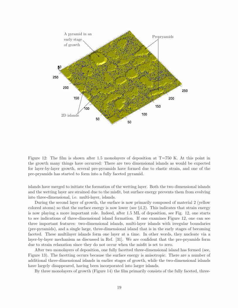
Figure 12: The film is shown after 1.5 monolayers of deposition at T=750 K. At this point inthe growth many things have occurred: There are two dimensional islands as would be expectedfor layer-by-layer growth, several pre-pyramids have formed due to elastic strain, and one of thepre-pryamids has started to form into a fully faceted pyramid.

islands have merged to initiate the formation of the wetting layer. Both the two dimensional islandsand the wetting layer are strained due to the misfit, but surface energy prevents them from evolvinginto three-dimensional, i.e. multi-layer, islands.

During the second layer of growth, the surface is now primarily composed of material 2 (yellowcolored atoms) so that the surface energy is now lower (see §4.2). This indicates that strain energyis now playing a more important role. Indeed, after 1.5 ML of deposition, see Fig. 12, one startsto see indications of three-dimensional island formation. If one examines Figure 12, one can seethree important features: two-dimensional islands, multi-layer islands with irregular boundaries(pre-pyramids), and a single large, three-dimensional island that is in the early stages of becomingfaceted. These multilayer islands form one layer at a time. In other words, they nucleate via alayer-by-layer mechanism as discussed in Ref. [31]. We are confident that the pre-pryamids formdue to strain relaxation since they do not occur when the misfit is set to zero.

After two monolayers of deposition, one fully facetted three-dimensional island has formed (see,Figure 13). The facetting occurs because the surface energy is anisotropic. There are a number ofadditional three-dimensional islands in earlier stages of growth, while the two-dimensional islandshave largely disappeared, having been incorporated into larger islands.

By three monolayers of growth (Figure 14) the film primarily consists of the fully faceted, three-

19

Pre-pryamids

Fully faceted island ✄✄✄✄✄✄✄✄✄✎

✟✟✟✟✟✟✟✟✟✟✟✟✟✟✙

❅❅❅❅❅❅❘

Figure 13: The film is shown after 2 monolayers of deposition at T=750 K. At this stage, most ofthe two dimensional islands have been consumed by the larger three dimensional islands. Thereare still several pre-pyramids and one fully faceted three dimensional island.

dimensional islands. It should be pointed out that this morphology is quite stable. Annealingsimulations will cause the very small islands to be incorporated into the bigger islands, but thebig islands do not appreaciably change their size or shape. Simliar results were reported in thesimulations of Aqua and Frisch [6] and the experiments of Berbezier et al. [49].

In summary, a wetting layer is first formed and then pre-pyramids are created by a layer-by-layernucleation mechanism that is driven by elastic strain. The pre-pyramids then evolve by surfacediffusion into faceted quantum dots. Our results confirm the work of Xiang et al. [31] who hadpredicted that quantum dots would form by a layer-by-layer nucleation mechanism. This indicatesthat one does not need to resort to the assumption (quoting from Ref. [42]) that “for strainedSiGe, the surface-energy anisotropy allows all orientations near (001), with the first facet being(105)” to provide a mechanism for faceted quantum dot formation. This scenerio is consistent withexperimental results.

The effect of temperature on the morphology is shown in Figures 15 and 16. Comparing Figures14 and 15, one observes that decreasing the temperature causes the island density to become largerand there are fewer fully facetted quantum dots. On the other hand, comparing Figures 14 and 16,we see that increasing the temperature results in all the quantum dots being facetted with a lowerdot density. We attribute these observation to the increased mobility that arises from increasingthe temperature. Finally, we show a simulation at a much higher temperature, namely T = 875 K.

20

Figure 14: The film is shown after 3 monolayers of deposition at T=750 K. Here most of the filmis covered in three dimensional, fully faceted island with a small number of pre-pyramids.

Here we observe an extremely rapid onset of facetted 3D islands. Figure 17 shows that at 1.4 MLno islands have formed and with just an additional 0.2 ML of deposited material a fairly large (13nm) facetted 3D island has grown.

4.4 Capping

Capping of quantum dots has been widely studied experimentally, for example [43, 44, 45, 46]. Ithas been established that the quantum dots can erode significantly during capping by a processthat is not well understood (e.g. Ref. [43]). In addition it has been observed in some experimentsthat during capping a fraction of the quantum dots evolve into ring-like structures (e.g. Refs.[44, 45, 46]). Our results not only are able to capture these phenomena, but they also provideinsight into the mechanisms behind them.

In our simulations we cap the film shown in Figure 14, which was grown at 750 K, with material1. We then use a capping temperature of 725 K, selecting this temperature so that a wide rangeof phenomena would be observed in one realization. If we had picked a much higher temperature,our simulations show that all of the dots will be almost completely eroded; if we had picked alower temperature, the morphology of the dots would have been unchanged during capping. Theseobservations are consistent with experimental results (e.g. Ref. [43]).

Figure 19 shows the morphology after the quantum dots displayed in Fig. 14 have been cappedwith 0.6 monolayers of material 1. We observe that the dots have noticeably eroded. Looking at

21

Figure 15: This figure shows the film after 3 monolayers of deposition. The conditions are identicalto the results shown in Figures 10 to 14 except the temperature has been lowered to 725 K. Thelowering of the temperature reduces atom mobility resulting in more islands that are smaller insize. In addition, the island shapes are more varied, with some rectangular and others square.

this figure, the mechanism behind this erosion becomes fairly clear. As the capping progresses, thewetting layer becomes more and more covered with material 1 (blue), which has a higher surfaceenergy that material 2 (yellow). This means there is a driving force for the material in the quantumdots to spread onto the wetting layer. A close examination of Figure 19 reveals that the dot materialis indeed getting wicked away. Figure 20 presents a cartoon version of this figure to clarify thismechanism. In this way the size of the dots are reduced. This mechanism will be intensifiedat higher temperatures due to greater mobility. This explains the experimental observation thatincreasing the temperature will increase dot erosion. It should be remarked that this conclusion isnot as obvious as it first sounds, because during the formation of the quantum dots increasing thetemperature will enhance dot formation: compare Figures 14, 15 and 16. Finally we point out thatReyes et al. [47] have argued that this mechanism is an important feature in liquid drop epitaxy.

Upon further capping, the dots become covered with material 1, and this mechanism is graduallyarrested. Further capping results in a situation where many dots have dissolved but several remain.Those that remain are surrounded by what is mainly material 1. Figure 21 shows the film after4.0 monolayers of capping material have been deposited. There are three quantum dots whose topsare still visible. It is interesting to note that the dot material (yellow colored atoms) is intermixedwith the capping material except for a ring-shaped region immediately near the edge of the dot.

22

Figure 16: This figure shows the film after 3 monolayers of deposition. The conditions are identicalto the results shown in Figures 10 to 14 except the temperature has been raised to 775 K whichincreases atom mobility resulting in fewer islands that are larger in size. In this case the shapes ofthe islands are more uniform.

This behavior has been reported in experiments [48].These dots are elastically compressed by the material 1 that surrounds them. In many cases it

is energetically preferable to relieve this strain energy by ejecting material from the center of thedots, thereby forming ring-like structures. Figure 22 shows an example of this process. Finally,Figure 23 shows a horizontal cross section after all of the dots have been completely capped. Thiscross section shows that many of the dots originally present have dissolved. Of the four thatsurvived, three evolved into ring-like structures. We have performed simulations over a wide rangeof parameter values, and we find these ring-like structures to be rather ubiquitous.

In closing, we mention that surface decomposition KMC has recently been applied to studycapping of GaAs dots by Ga1−xInxAs [48]. In that paper the reader will find detailed comparisonsof simulations using the algorthim presented here with experimental results.

5 Summary

In this paper we have offered an approximation to a well established KMC model for heteroepitaxialgrowth. The key to this approximation is that the elastic interaction of low coordinated atoms withthe rest of crystal is sufficiently weak that it may be ignored. The resulting model still satisfies

23

Prepryamid

2D islands

✄✄✄✄✄✄✄✄✄✄✄✄✎

✻

�������������

����✒

Figure 17: This figure shows the film after 1.4 monolayers of deposition. The conditions are identicalto the results shown in Figures 10 to 14 except the temperature has been raised to 875 K. At thispoint only one small pre-pryamid has formed. The elevated temperature inhibits the formation ofpre-pryamids due to entropic effects.

detailed balance, and its implementation results in simulation speeds that are close to fifteen timesfaster. Various tests quantitatively reveal that this approximation is quite faithful to the evolutionof the original model. One of these tests implies that the alignment that occurs in the stackingof quantum dots results from interactions between islands and buried dots and not from adatom-buried dot interactions as suggested by other investigations. It is shown that our method cansimulate Stranski-Krastanov growth. We provide evidence that faceted 3D islands result from thelayer-by-layer nucleation of pre-pyramids and fully faceted islands result from anisotropic surfacediffusion. The capping of islands is also studied, and it is shown that capping causes erosion of thequantum dots because the dot material is used to replenish the wetting layer. Our simulations arealso able to capture the formation of ring-like structures.

Acknowledgments

We thank J.N. Aqua, A. Baskaran, P. Koenraad, J.M. Millunchick, K. Reyes, Y. Saito, and V. Sih,for helpful conversations. This work was supported, in part, by NSF support grants DMS-0810113,DMS-0854870, and DMS-1115252.

24

Figure 18: The film is shown after 1.6 monolayers of deposition at T=875 K. This demonstratesthe rapid growth of a pre-pryamid into a fully faceted, three dimensional island.

References

[1] X. Niu, R. Vardavas, R.E. Caflisch, and C. Ratsch, Phys. Rev. B 74, Art. No. 193403 (2006).

[2] X. Niu, Y.L. Lee, R.E. Caflisch, and C. Ratsch, Phys. Rev. Lett. 101, Art. No. 086103 (2008).

[3] C. Ratsch, J. Devita, and P. Smereka, Phys. Rev. B 80, Art. No. 155309 (2009).

[4] Wise, S.M., Lowengrub, J.S., Kim, J.S., Johnson, W.C., Superlattices Microstruct. 36, 293304(2004).

[5] Wise, S.M., Lowengrub, J.S., Kim, J.S., Thornton, K., Voorhees, P.W., Johnson, W.C., Appl.

Phys. Lett. 87, Art. No. 133102 (2005).

[6] J.N. Aqua and T. Frisch, Phys. Rev. B 82 2555 (2010).

[7] M. Ortiz, E.A. Repetto, and H. Si, J. Mech. Phys. Sol. 47, 697-730 (1999).

[8] B.J. Spencer, P.W. Voorhees, and S.H. Davis, Phys. Rev. Lett. 67, 3696-3699 (1991).

[9] Y. Tu and J. Tersoff, Phys. Rev. Lett. 93 216101 (2004).

[10] C.H. Lam, C.K. Lee, and L.M. Sander, Phys. Rev. Lett. 89, 16102 (1-4) (2002).

25

Dot material thathas been wickedonto the substrate✄✄✄✄✄✄✄✄✄✄✄✄✄✎

✟✟✟✟✟✟✙

��

��

��

��

��

��

��

��

��✠

Figure 19: The film shown in Figure 14 is capped with material 1 at T=725 K. This figure showsthe result after 0.6 monolayers of capping material (blue colored atoms) have been deposited. Thereader should notice that the wetting layer which was primarily compose of material 2 (yellowcolored atoms, see, Figure14) now has a high concentration of material 1 (blue colored atoms).This results in a surface with a higher surface energy which in turn provides a driving force for dotmaterial to cover the surface. This figure clearly shows the quantum dots have been reduced in sizedue to dot material being wicked away to replenish the wetting layer.

[11] Lee S., Caflsich R.E., Lee Y.J. SIAM J. Appl. Math. 66, 17491775 (2006).

[12] M.T. Lung, C.H. Lam, and L.M. Sander, Phys. Rev. Lett. 95 Art. No. 086102 (2005).

[13] G. Russo and P. Smereka, J. Comput. Phys. 214, 809-828 (2006).

[14] G. Russo and P. Smereka, Multiscale Model. Simu. 5, 130-148 (2006).

[15] T.P. Schulze and P.Smereka, J. Mech. Phys. Solids. 57 521-538 (2009).

[16] T.P. Schulze and P. Smereka, Comm. Comput. Phys. 10 1089-1112 (2011).

[17] D. Leonard, K. Pond, and L.M. Petroff, Phys. Rev. B 50 11687-11692 (1994).

[18] R.J. Asaro and W.A. Tiller, Metall. Trans. 3 1789 (1972).

[19] M.A. Grinfeld, J. Nonlinear Sci. 3 35 (1993).

26

Dot material thathas been wickedonto the substrate✄✄✄✄✄✄✄✄✄✄✄✄✄✎

✟✟✟✟✟✟✙

��

��

��

��

��

��

��

��

��✠

Figure 20: This is a cartoon of Figure 19 that serves to emphasize how the material in the dots iswicked on to the substrate.

[20] J. Tersoff, Phys. Rev. B 43, 9377-9380 (1991).

[21] A. Baskaran and P. Smereka, J. Appl. Phys. 111 Art. No. 044321 (2012).

[22] A. Baskaran, J. Devita, and P. Smereka, Contin. Mech. Thermo. 22 1-26 (2010).

[23] C.H. Lam, J. Applied Physics 108, Art. No. 064328, (2010).

[24] C.H. Lam, Physical Review E 81, Art. No. 021607, (2010).

[25] B.G. Orr, D.A. Kessler, C.W. Snyder, and L.M. Sander, Europhysics Lett. 19, 33-38 (1992).

[26] L.M. Sander, Advanced Condensed Matter Physics, Cambridge University Press, Cambridge(2009). (see page 61).

[27] C. Rottman and M. Wortis, Phys. Rev. B 24, 6274-6277 (1981).

[28] J.P. Devita, L.M. Sander, and P. Smereka, Phys. Rev. B 72, Art. No. 205421 (2005).

[29] C. Rottman and M. Wortis, Phys. Rev. B 29, 328-339 (1984).

[30] H.J. Leamy, G.H. Gilmer, and K.A. Jackson, Statistical Thermodynamics of Clean Surfaces,in Surface Physics of Material vol. 1, ed J.M. Blakely, Academic Press, New York 1975.

27

dots surroundedby cappingmaterial

Ring ofdepleteddot material

❄

✟✟✟✟✟✟✟✟✟✟✟✟✟✟✟✟✟✟✟✟✟✟✟✟✟✙

✓✓

✓✓

✓✓

✓✓

✓✓

✓✓

✓✓

✓✓✴

❅❅❅❅❅❘

Figure 21: This shows the result after 4 ML of capping at T=725 K. This figure shows three dotsthat have been completely surrounded by capping material. The surrounded dots are now beingcompressed by the capping material which greatly increases their elastic energy.

[31] R.X. Xiang, M.T. Lung, C.H. Lam, Physical Review E 82, Art. No. 021602 (2010).

[32] W.K. Burton, N. Cabrera, and F.C. Frank, Trans. R. Soc. London Ser. A 243, 299 (1951).

[33] T.P. Schulze, P. Smereka and W. E, to Epitaxial Growth, J. Comp. Phys. 189 197-211 (2003).

[34] I.V. Markov, Crystal growth for Beginners: Fundamentals of Nucleation, Crystal Growth, andEpitaxy, World Scientific (2003).

[35] M. Biehl, M. Ahr, W. Kinzel, and F. Much, Thin Solid Films 428, 52-55 (2003).

[36] W. Guo, T.P. Schulze and W. E, Simulation of Impurity Diffusion in a Strained NanowireUsing Off-lattice KMC, Comm. Comp. Phys. 2 164-176 (2007).

[37] J.L. Blue, I. Biechl, and F. Sullivan, Phys. Rev. E 51 876 (1995).

[38] J. Tersoff, C. Teichert, and M.G. Lagally, Phys. Rev. Lett. 76 1675-1678 (1996).

[39] R.J. Jaccodine, J. Electrochemical Soc. 110 524-527 (1963).

[40] M.S. Levine, A.A. Golovin, S.H. Davis, and P.W. Voorhees, Phys. Rev. B 75 Art. No. 205312(2007).

28

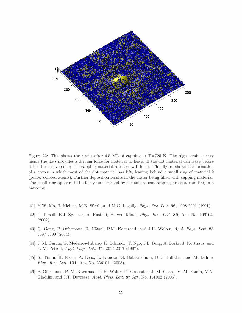
Figure 22: This shows the result after 4.5 ML of capping at T=725 K. The high strain energyinside the dots provides a driving force for material to leave. If the dot material can leave beforeit has been covered by the capping material a crater will form. This figure shows the formationof a crater in which most of the dot material has left, leaving behind a small ring of material 2(yellow colored atoms). Further deposition results in the crater being filled with capping material.The small ring appears to be fairly undisturbed by the subsequent capping process, resulting in ananoring.

[41] Y.W. Mo, J. Kleiner, M.B. Webb, and M.G. Lagally, Phys. Rev. Lett. 66, 1998-2001 (1991).

[42] J. Tersoff. B.J. Spencer, A. Rastelli, H. von Kanel, Phys. Rev. Lett. 89, Art. No. 196104,(2002).

[43] Q. Gong, P. Offermans, R. Notzel, P.M. Koenraad, and J.H. Wolter, Appl. Phys. Lett. 85

5697-5699 (2004).

[44] J. M. Garcia, G. Medeiros-Ribeiro, K. Schmidt, T. Ngo, J.L. Feng, A. Lorke, J. Kotthaus, andP. M. Petroff, Appl. Phys. Lett. 71, 2015-2017 (1997).

[45] R. Timm, H. Eisele, A. Lenz, L. Ivanova, G. Balakrishnan, D.L. Huffaker, and M. Dahne,Phys. Rev. Lett. 101, Art. No. 256101, (2008).

[46] P. Offermans, P. M. Koenraad, J. H. Wolter D. Granados, J. M. Garca, V. M. Fomin, V.N.Gladilin, and J.T. Devreese, Appl. Phys. Lett. 87 Art. No. 131902 (2005).

29

50 100 150 200 250

50

100

150

200

250

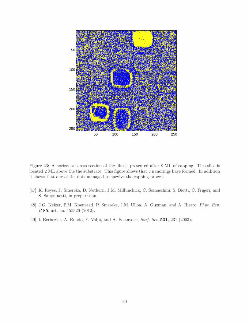
Figure 23: A horizontal cross section of the film is presented after 8 ML of capping. This slice islocated 2 ML above the the substrate. This figure shows that 3 nanorings have formed. In additionit shows that one of the dots managed to survive the capping process.

[47] K. Reyes, P. Smereka, D. Nothern, J.M. Millunchick, C. Somaschini, S. Bietti, C. Frigeri, andS. Sanguinetti, in preparation.

[48] J.G. Keizer, P.M. Koenraad, P. Smereka, J.M. Ulloa, A. Guzman, and A. Hierro, Phys. Rev.B 85, art. no. 155326 (2012).

[49] I. Berbezier, A. Ronda, F. Volpi, and A. Portavoce, Surf. Sci. 531, 231 (2003).

30