knock prediction with reduced reaction …19255/fulltext01.pdf · knock, combustion, kinetics,...
TRANSCRIPT

KNOCK PREDICTION WITHREDUCED REACTION ANALYSIS
Master’s thesisperformed in Vehicular Systems
byTOMAS LIDHOLM
Reg nr: LiTH-ISY-EX-3466-2003
22nd August 2003


KNOCK PREDICTION WITHREDUCED REACTION ANALYSIS
Master’s thesis
performed in Vehicular Systems,Dept. of Electrical Engineering
at Linkopings universitet
by TOMAS LIDHOLM
Reg nr: LiTH-ISY-EX-3466-2003
Supervisor: Gunnar CedersundLinkopings Universitet
Ylva NilssonLinkopings Universitet
Examiner: Associate professor Lars ErikssonLinkopings Universitet
Linkoping, 22nd August 2003


Avdelning, InstitutionDivision, Department
DatumDate
Sprak
Language
¤ Svenska/Swedish
¤ Engelska/English
¤
RapporttypReport category
¤ Licentiatavhandling
¤ Examensarbete
¤ C-uppsats
¤ D-uppsats
¤ Ovrig rapport
¤URL for elektronisk version
ISBN
ISRN
Serietitel och serienummerTitle of series, numbering
ISSN
Titel
Title
ForfattareAuthor
SammanfattningAbstract
NyckelordKeywords
In the report a model using a reduced reaction analysis has been usedto see if it is possible to use it to predict if and when knock occurs in anSI-engine. The model is based on n-heptane combustion, but it is usedfor iso-octane. The model was supposed to be able to adapt to differentfuels, but was not able to do so in this case. Further, the model has beencompared to an existing method for predicting knock, known as knockindex and it has shown that no big advantages can be found usingthe new model. It can predict if knock occurs from both simulatedand measured pressure curves but with simulated input virtually nodetection time can be predicted. Even though it can predict if knockoccurs with a good reliability it is not an improvement compared tothe knock index.
Vehicular Systems,Dept. of Electrical Engineering581 83 Linkoping
22nd August 2003
—
LITH-ISY-EX-3466-2003
—
http://www.vehicular.isy.liu.sehttp://www.ep.liu.se/exjobb/isy/2003/3466/
KNOCK PREDICTION WITH REDUCED REACTION ANALYSIS
KNACKPREDIKTION MED HJALP AV REDUCERAD REAK-TIONSANALYS
TOMAS LIDHOLM
××
Knock, Combustion, Kinetics, Prediction, Reactions, Engine


Abstract
In the report a model using a reduced reaction analysis has been usedto see if it is possible to use it to predict if and when knock occurs in anSI-engine. The model is based on n-heptane combustion, but it is usedfor iso-octane. The model was supposed to be able to adapt to differentfuels, but was not able to do so in this case. Further, the model has beencompared to an existing method for predicting knock, known as knockindex and it has shown that no big advantages can be found usingthe new model. It can predict if knock occurs from both simulatedand measured pressure curves but with simulated input virtually nodetection time can be predicted. Even though it can predict if knockoccurs with a good reliability it is not an improvement compared tothe knock index.
Keywords: Knock, Combustion, Kinetics, Prediction, Reactions, En-gine
v
Thesis outline
This thesis consists of five chapters. The first chapter is an introductionto the problem, and to combustion engines and knock. The secondchapter deals with the chemistry that most of the model is based on,explaining the theory used in the model. In the third chapter, themodel as it has been used is described, together with a descriptionof how it was implemented in Matlab. The fourth chapter shows thevalidation of the model, and also different adaptions that was tried toimprove the model. In the fifth chapter the results of the model, anda comparison with an existing model, is shown and discussed. In thesixth chapter conclusions of the work are sumarized
Acknowledgment
I would like to thank everyone who has helped me get this through tothe end. Specially, I want to thank my supervisors, Ylva and Gunnar,for all the help and ideas they have come up with. Further, I wouldlike to thank the people at the Division of Combustion Physics, LundInstitute of Technology, for supplying the model to get me started. Iwould also like to thank all the people at the Department of Vehicularsystems, Linkopings university, for all the help and company they havegiven me.
vi
Contents
Abstract v
Preface and Acknowledgment vi
1 Introduction 11.1 SI-engines . . . . . . . . . . . . . . . . . . . . . . . . . . 1
1.1.1 The working principle of an SI-engine . . . . . . 21.1.2 Cycle to cycle variations . . . . . . . . . . . . . . 3
1.2 Knock and its consequences . . . . . . . . . . . . . . . . 41.2.1 Two-zone models . . . . . . . . . . . . . . . . . . 51.2.2 Octane and cetane numbers . . . . . . . . . . . . 5
2 Chemistry 62.1 Chemical kinetics . . . . . . . . . . . . . . . . . . . . . . 6
2.1.1 From reaction to equation . . . . . . . . . . . . . 72.2 Chemical equilibrium . . . . . . . . . . . . . . . . . . . . 82.3 The chemistry of combustion . . . . . . . . . . . . . . . 8
3 Model and structure 93.1 The model . . . . . . . . . . . . . . . . . . . . . . . . . . 9
3.1.1 Modified Arrhenius expressions . . . . . . . . . . 103.1.2 Temperature . . . . . . . . . . . . . . . . . . . . 103.1.3 Initial temperature . . . . . . . . . . . . . . . . . 113.1.4 Specific heat . . . . . . . . . . . . . . . . . . . . 11
3.2 The program . . . . . . . . . . . . . . . . . . . . . . . . 123.2.1 CHEPP . . . . . . . . . . . . . . . . . . . . . . . 133.2.2 The shell . . . . . . . . . . . . . . . . . . . . . . 143.2.3 Definition of substances and reactions . . . . . . 143.2.4 Differential equations . . . . . . . . . . . . . . . 153.2.5 Solver . . . . . . . . . . . . . . . . . . . . . . . . 16
vii

4 Evaluation of model 174.1 Changing parameters . . . . . . . . . . . . . . . . . . . . 19
4.1.1 Changing the cetane number . . . . . . . . . . . 204.1.2 Further changes . . . . . . . . . . . . . . . . . . . 224.1.3 Parameter optimization . . . . . . . . . . . . . . 244.1.4 Optimization method . . . . . . . . . . . . . . . 254.1.5 Optimization results . . . . . . . . . . . . . . . . 254.1.6 Changing the A and E values . . . . . . . . . . . 26
5 Analysis 315.1 Detection . . . . . . . . . . . . . . . . . . . . . . . . . . 315.2 Time of knock . . . . . . . . . . . . . . . . . . . . . . . . 335.3 Knock index . . . . . . . . . . . . . . . . . . . . . . . . . 35
6 Conclusions 376.1 Future work . . . . . . . . . . . . . . . . . . . . . . . . . 38
References 39
Notation 41
A Manual for the program 43
B Validation data 45
viii
Chapter 1
Introduction
The purpose of this masters thesis is to evaluate the possibilities touse a reduced reaction analysis to predict knock in internal combustionengines. The objective is to find a model that can predict if and whenknock occurs for a given pressure curve. This method will be comparedto an existing method, known as knock index, to see if the older methodcan be improved.
There is also an interest to find out more about models of reducedreaction analysis, and whether these can be used without to much lossof accuracy. The method used in this thesis is one of the simplestpossible, reducing the number of different reactions taking place tofour. Totally there are eight different substances involved.
A notation with all abbreviations and symbols used can be foundin the end of the report.
1.1 SI-engines
A spark ignited (SI), engine, is the most common type of engine used inmodern cars. Other engine types are diesel and Homogeneous ChargeCompression Ignition (HCCI), though the HCCI engine is only for re-search and has not yet reached production. In an SI-engine, self ignitionof the fuel is a limiting factor. Self ignition in an SI-engine is commonlyreferred to as knock. This will be described in section 1.2 but to un-derstand the consequences better, it is best to know the basics of howan SI-engine works. A short description of the basics of an SI enginewill be provided, for more information see [10].
1

2 Chapter 1. Introduction
−400 −300 −200 −100 0 100 200 300 400−1
0
1
2
3
4
5
6x 10
6
Crank angle degrees
Pre
ssur
e [P
a]
Figure 1.1: A typical plot of the pressure in the cylinder for the four-stroke cycle.
1.1.1 The working principle of an SI-engine
The four-stroke cycle is a way of describing the functionality of an SI-engine. The cycle is divided into four parts, taking two full revolutionsof the piston. The four parts are intake, compression, expansion andexhaust.
In the intake phase (TDC-BDC) the piston moves down while theinlet valve is open and a mixture of gasoline and air is inhaled into thecylinder. When the piston reaches its lowest position the compressionphase starts.
In the compression phase (BDC-TDC) the inlet valve is closed andthe piston is moving up, compressing the fuel/air mixture. At a certainpoint, about 25◦ BTDC (before TDC), a spark ignites the fuel. As theflame expands through the cylinder the temperature, and hence alsothe pressure, rises.
When the piston reaches its top position the expansion phase (TDC-BDC) begins. The combustion continues through the beginning of thisphase, giving more energy to the system. This is the phase where usefulwork is put out from the engine. The high pressure in the cylinderpushes the piston down, creating a force that moves the vehicle forward.At the end of this phase the exhaust valve is opened to let all theresidual gases out of the combustion chamber.
In the last phase, the exhaust phase (BDC-TDC), of the combus-tion, the piston moves up, pushing all the residual gases out of the

1.1. SI-engines 3
−100 −50 0 50 100 1500
1
2
3
4
5
6
7
x 106
Crank angle degrees
Pre
ssur
e [P
a]
Figure 1.2: Cycle to cycle variations in the cylinder, under steady stateconditions
cylinder. When the piston reaches TDC, a new cycle begins. In fig-ure (1.1) a plot of the pressure as a function of crank angle degreesis shown. It starts at −360◦ (TDC) and is completed two revolutionslater, at 360◦. The different phases do not have to start exactly atBDC or TDC. These angles are just an approximation. The valves donot open and close at exactly BDC or TDC, but rather close to them.
1.1.2 Cycle to cycle variations
The pressure varies a lot between different cycles. This occurs evenwhen the engine is working under steady state conditions, i.e. all con-trollable parameters are held constant. In figure 1.2, a number of con-secutive cycles are shown, and as can be seen, the pressure varies be-tween cycles. According to [10] there are three major reasons why thisoccurs.• Variations in the gas motion in the cylinder.• Variations in the amount of fuel, air and recycled gases causes
the amount of energy in the cylinder to vary from one cycle toanother.
• Spatial variations in the concentration of air, fuel and recycledgases.
These variations are a problem since they limit engine efficiency andmakes it harder to control the engine. Even though the engine is run-ning safely, at operating points that should not cause knock, occasional
4 Chapter 1. Introduction
0 0.1 0.2 0.3 0.4 0.5
3.5
4
4.5
5
5.5
6
6.5
x 106
Crank angle degrees
Pre
ssur
e [P
a]
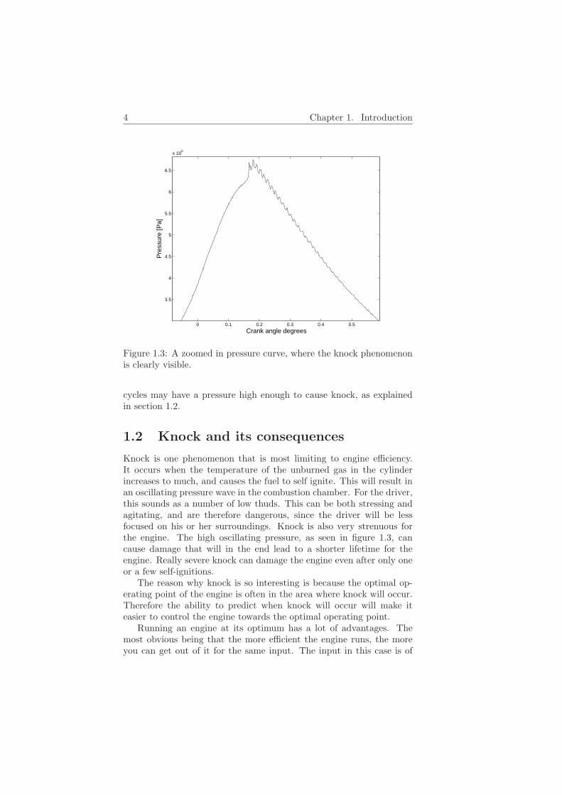
Figure 1.3: A zoomed in pressure curve, where the knock phenomenonis clearly visible.
cycles may have a pressure high enough to cause knock, as explainedin section 1.2.
1.2 Knock and its consequences
Knock is one phenomenon that is most limiting to engine efficiency.It occurs when the temperature of the unburned gas in the cylinderincreases to much, and causes the fuel to self ignite. This will result inan oscillating pressure wave in the combustion chamber. For the driver,this sounds as a number of low thuds. This can be both stressing andagitating, and are therefore dangerous, since the driver will be lessfocused on his or her surroundings. Knock is also very strenuous forthe engine. The high oscillating pressure, as seen in figure 1.3, cancause damage that will in the end lead to a shorter lifetime for theengine. Really severe knock can damage the engine even after only oneor a few self-ignitions.
The reason why knock is so interesting is because the optimal op-erating point of the engine is often in the area where knock will occur.Therefore the ability to predict when knock will occur will make iteasier to control the engine towards the optimal operating point.
Running an engine at its optimum has a lot of advantages. Themost obvious being that the more efficient the engine runs, the moreyou can get out of it for the same input. The input in this case is of

1.2. Knock and its consequences 5
course gasoline, and therefore an efficient running engine will reduce theamount of gasoline it uses. This will lead to a reduced oil consumption,which is a must since the earths fuel supplies are being depleted. Areduced fuel consumption will also reduce the discharge of pollutantssuch as NOx and CO2, which is very good for the environment, andwill reduce the contribution to the green house effect.
1.2.1 Two-zone models
When modeling knock, a common way is to use a thermodynamic two-zone model. The two zones are for the burned and unburned partsof the air/fuel mixture. The zones are separated by the propagatingflame front, that is assumed to be infinitesimal. The two zones havethe same pressure, but different temperature and chemical composition.The models include heat and mass transfers between the zones as wellas heat transfer to the surroundings. The model used in this thesis isa two-zone model, but since the only interest is in the unburned zone,no model for the burned zone is made. However, when knock occurs,and the fuel in the unburned zone ignites, the gas will no longer beunburned, but it is still treated as a separate zone to simplify the model.
1.2.2 Octane and cetane numbers
The octane number is a measure on how likely the fuel is to self-ignite.A fuel that is prone to knock will have a low octane number, and afuel that is not as likely to knock will have a higher. The numberis defined after the two fuels iso-octane and n-heptane. Iso-octane isdefined as 100 and n-heptane as 0 on the octane scale. If a fuel has anoctane rating of 95, the fuel is as likely to knock as a mixture of 95%of iso-octane and 5% of n-heptane.
The cetane number is the opposite to the octane, in the sense thatit has a higher value the more prone a fuel is to self-ignite. There isnot, however, any easy correlation between the two values. The cetanenumber is defined as the octane number, but instead of iso-octane andn-heptane, the definition uses cetane, C16H34, a substance that ignitesvery easy, and alpha-methylnapthalene, C10H7CH3, a substance thatis very hard to ignite. According to [14] , the cetane numbers for iso-octane and n-heptane are about 5 and 60 respectively , but the relationis not linear. More information about the correlation between octaneand cetane numbers can be found in [14].
Chapter 2
Chemistry
The combustion process can be well described with chemistry and ther-modynamics. In this chapter there will be an introduction to the differ-ent parts of the chemistry involved. In section 2.1 the non-steady statechemistry, or chemical kinetics, will be brought up, while in section 2.2the steady state chemistry is discussed. In section 2.3 the more combus-tion specific chemistry will be discussed. A more thorough explanationof the chemistry involved in combustion can be found in [5].
2.1 Chemical kinetics
Chemical kinetics are used to describe a reacting system, where changesoccur constantly. A reaction is described by the reactants and products,and a reaction rate, that is a measurement of the speed with which areaction occurs. A reaction is often written as:
A + B À C + D (2.1)
In some cases, the reaction is not very likely to occur in both directions.In these cases, the reactions can be written as one-way reactions on thefollowing form:
A + B → C + D (2.2)
A, B, C and D are arbitrary chemical substances.The reaction rates are calculated using the Arrhenius function. The
forward reaction is described by:
kf = ATne−E
RT (2.3)
where A, n and E are tabulated values. E is the reactions activationenergy, an energy level that the substances must reach to start.
6
2.1. Chemical kinetics 7
The backward reaction rate can be calculated using the forwardreaction rate and the equilibrium concentration for the substance as:
kb =kf
K(2.4)
2.1.1 From reaction to equation
To be able to calculate concentrations as a function of time, a method totransform the reactions into differential equations must be used. Thismethod is described at length in [5].
The rate with which the reactions occur depends on two things.The first is the reaction rate, k, from the Arrhenius equation (2.3).The other factor is the concentration of the reacting substances. Thehigher the concentration the more they react. For an arbitrary reaction
A + B À C (2.5)
with reaction rates kf and kb the differential equations for the concen-trations are formed as
d[A]dt
=d[B]dt
= −d[C]dt
= −kf [A][B] + kb[C] (2.6)
As an example, consider the (one-way) reaction:
H2 + M → 2H + M (2.7)
Here, the substance H2 reacts, or rather collides, with a neutral sub-stance M and splits into two H atoms. M is usually used to representthe total of all molecules in a system and are often a part of a reactionas a catalyst, since many reactions will not occur unless a collision hastaken place. The change in concentration of H2 and H molecules canin this case be written as:
d[H2]dt
= −k[H2][M ] (2.8)
d[H]dt
= 2k[H2][M ] (2.9)
where k is the reaction rate for the reaction.The total reaction rate with which the reaction occurs, in this case
k[H2][M ] are often denoted with the Greek letter ω. This is only definedfor one-way reactions, and therefore the arbitrary reaction (2.5) willhave two different ω-values. One for the forward reaction, ωf and onefor the backward, ωb. With this definition equations (2.8) and(2.9) canbe written as
d[H2]dt
= −ω (2.10)
d[H]dt
= 2ω (2.11)

8 Chapter 2. Chemistry
but equation (2.6) is written as
d[A]dt
=d[B]dt
= −d[C]dt
= −ωf + ωb (2.12)
For a more complex system, containing more than one reaction, thedifferential equation will contain one element for each reaction the sub-stance is partaking in. For example a system with two reactions, 1 and2. In the first reaction, one molecule of H2 is a reactant, and in thesecond, one molecule is produced. The expression for calculation of theconcentration would then be:
d[H2]dt
= −ω1 + ω2 (2.13)
2.2 Chemical equilibrium
If a reaction, or a number of reactions, can go on for a long time, the sys-tem will reach chemical equilibrium. Long being from mere millisecondsup to thousands of years, depending on factors such as temperature,pressure and the reacting substances. Chemical equilibrium means thatthe concentration of the substances are constant. This is not equivalentwith a system where no reactions are taking place. There can be a lotof reactions happening, but they will not change the concentration ofany substance. That is, for every reaction ’taking’ from a substance,another reaction must be ’giving’. The system in equilibrium is af-fected by outer factors, such as pressure and temperature. Therefore, asystem in chemical equilibrium will probably not be in chemical equi-librium if the temperature changes. For more information on how tocalculate chemical equilibrium, see [2].
2.3 The chemistry of combustion
The combustion of iso-octane is a very complex chemical system. Thereactions included in the model in chapter 3 might seem easy and fewbut in such a reduced system most of the interim stages are disregardedsince the substances thus created only exist for a very short time. Intotal there are over 2500 of these interim substances and they takepart in several thousands of reactions. A system this big will be verytime-consuming to solve, and therefore a reduction of the system isnecessary. There are several possible ways to reduce the reactions, andsome of those are discussed in [11, 13]. The model used here are evensimpler than those discussed in the mentioned articles. A full reviewof the chosen model is given in chapter 3.

Chapter 3
Model and structure
3.1 The model
The model chosen for this application is one of the simplest possiblewhen modeling combustion. It is the four step method found in [9].This model is based on the combustion of n-heptane and the demandsset by Muller [9] is to describe the kinetics of n-heptane combustion asgood as possible. The main goal is however to describe diesel fuels, andto do this the cetane number has been included in the model to be ableto adapt the model for different types of fuel. Thus it should be possibleto use the model when modeling iso-octane combustion. The goal isto have a physically correct model that can discover knock through achange in the chemical concentrations. Especially the amount of burntfuel should be very different between the cycles with and without knock.
The model involves only four reactions, containing eight substances,and thus giving rise to eight differential equations. The reactions are:
n − C7H16 → 3C2H4 + CH3 + H (3.1)3C2H4 + CH3 + H + 11O2 + M → 7CO2 + 8H2O + M (3.2)
n − C7H16 + 2O2 À HO2C7H13O + H2O (3.3)HO2C7H13O + H2O + 9O2 → 7CO2 + 8H2O (3.4)
In addition to the eight differential equations formed from the reac-tions, a ninth is formed for the temperature. This is a very importantpart of the model, since the reaction rates are very dependent on thetemperature.
There are several different isomers of the substance HO2C7H13Obut in this model the isomer n − HO2C7H13O has been used.
9
10 Chapter 3. Model and structure
3.1.1 Modified Arrhenius expressions
This model does not use the Arrhenius expression described in section2.1, but a slightly modified version of it, to calculate the reaction ratesof the system. For easier overlook, the reactions (3.1) to (3.4) are heredenoted reaction 1 to 4, with reaction 3 being split into 3f and 3b, forits forward and backward reaction.
There are two major differences in this model compared to the orig-inal Arrhenius expression. The first is that instead of the temperaturethe pressure is used in the factor that is not in the exponent. Theother difference is that in reaction 4 a factor (CN
60 )2 is included. This isbecause the model is based on n-heptane combustion, and to simulateanother fuel, Muller [9] states that this can be done by changing thecetane number. The cetane number of the fuel is used as input to theCN factor. The cetane number of n-heptane is 60, so in that case thefactor is one, but since this model is used for iso-octane combustion, itwill have an effect.
The total reaction rates for the reactions are:
ω1 = [n − C7H16]A1e−E1/RT (3.5)
ω2 = [C2H4][CH3][H][O2][M ]A2e−E2/RT (3.6)
ω3f = [n − C7H16][O2]p−1.75A3fe−E3f /RT (3.7)
ω3b = [HO2C7H13O][H2O]p−1.75A3be−E3b/RT (3.8)
ω4 = [HO2C7H13O][H2O][O2](
CN
60
)2
A4e−E4/RT (3.9)
The values Ai and Ei are
Reaction A E[kJ/mol]1 9.0 · 108 150.02 7.0 · 1015 60.03f 1.0 · 1020 160.03b 5.0 · 1025 310.04 1.0 · 1013 110.0
where the unit of A depends on which reaction it is. The unit of Ai isadapted so that the unit of ωi is mol/(m3 · sec). Thus the unit of Ai
is(
m3
mol
)xi−1 1sec , where xi equals the number of reacting substances in
reaction i.
3.1.2 Temperature
The temperature model is very important, as explained earlier, and itis also the most complex part of the total model. The model used can
3.1. The model 11
be found in [1]. The expression for calculation of the temperature is:
ρucp,udTu
dt=
dp
dt−
Ns∑j=1
hjMj,u
Nr∑k=1
νj,kωk + αAw
Vu(Tw − Tu) (3.10)
In this model the last part, αAw
Vu(Tw − Tu), is neglected to simplify the
model further. The term is a model for the heat loss from the unburnedsection to the wall of the cylinder. By removing this term, the modelprobably gets less accurate, and a further improvement of the modelmight include adding this term back to the equation.
The density of the unburned zone, ρu is calculated as:
ρu =mu
Vu= p
Mu
RTu
(3.11)
3.1.3 Initial temperature
In the beginning, the initial temperature was set to 400K. The initialtemperature can, however, vary and can not be set as constant in amore precise experiment. Such considerations as residual gases must betaken when calculating the temperature. For this experiment this wasnot of a major importance, and tests were made with different initialtemperatures and it was shown that it did not effect the importantparts of the model.
3.1.4 Specific heat
The specific heat, cp, of a substance is defined as:
cp =(
∂H
∂T
)p,m
(3.12)
where H is the free energy of the substance. Due to the definition thespecific heat for an entire system is a bit complex to calculate. Thecorrect way to calculate the total cp for the unburned gases is:
cp,u =(
∂
∂T
(hu
Mu
))p,m
=1
Mu
(∂hu
∂T
)p,m
− hu
M2u
(∂Mu
∂T
)p,m
(3.13)
where(
∂hu
∂T
)p,m
=∑
i
(xicp,i + hi
(∂xi
∂T
)p
)
(∂Mu
∂T
)p,m
=∑
i
Mi
(∂xi
∂T
)p
12 Chapter 3. Model and structure
500 1000 1500 2000 2500 300070
80
90
100
110
120
130
140
150
Temperature [K]
Spe
cific
hea
t, c p
Full modelSimplified model
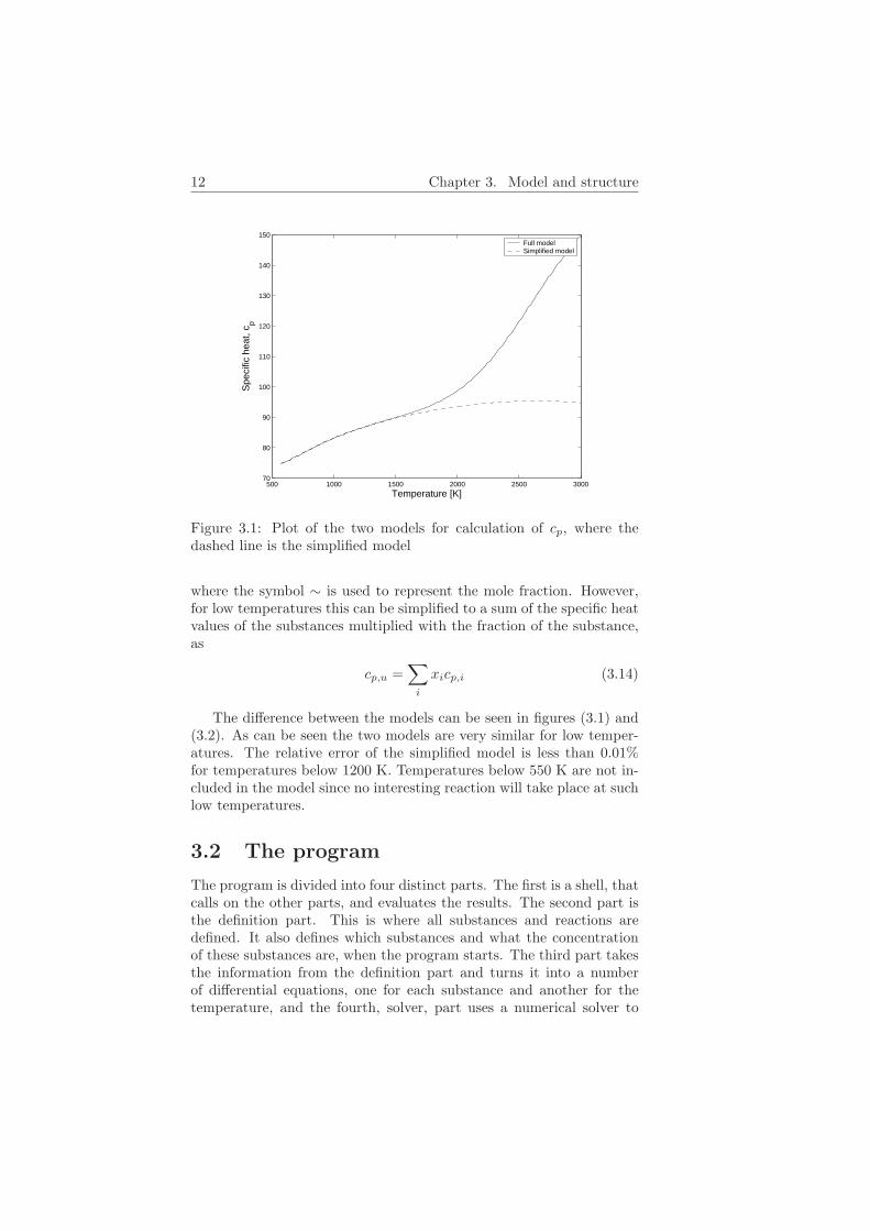
Figure 3.1: Plot of the two models for calculation of cp, where thedashed line is the simplified model
where the symbol ∼ is used to represent the mole fraction. However,for low temperatures this can be simplified to a sum of the specific heatvalues of the substances multiplied with the fraction of the substance,as
cp,u =∑
i
xicp,i (3.14)
The difference between the models can be seen in figures (3.1) and(3.2). As can be seen the two models are very similar for low temper-atures. The relative error of the simplified model is less than 0.01%for temperatures below 1200 K. Temperatures below 550 K are not in-cluded in the model since no interesting reaction will take place at suchlow temperatures.
3.2 The program
The program is divided into four distinct parts. The first is a shell, thatcalls on the other parts, and evaluates the results. The second part isthe definition part. This is where all substances and reactions aredefined. It also defines which substances and what the concentrationof these substances are, when the program starts. The third part takesthe information from the definition part and turns it into a numberof differential equations, one for each substance and another for thetemperature, and the fourth, solver, part uses a numerical solver to

3.2. The program 13
500 1000 1500 2000 2500 30000
5
10
15
20
25
30
35
40
Temperature [K]
Rel
ativ
e er
ror
in s
peci
fic h
eat,
c p (%
)
Figure 3.2: Plot of the relative error of the reduced model. As canbe seen the models differ very little for temperatures below 1500K andeven for temperatures below 2000K the relative error is less then 5%
solve the differential equations. It is the results from these equationsthat are evaluated by the shell. A scheme of the program is includedin figure 3.3.
The program is made to be able to work for any set of reactions andsubstances selected. It can therefore be used to simulate any model ofcombustion, not only the one shown in this report. in appendix A amanual on how to use the program can be found.
3.2.1 CHEPP
For calculation of chemical equilibrium, CHEPP or CHemical Equilib-rium Program Package has been used. CHEPP uses the NASA polyno-mial form, see [8], to calculate the thermo chemical properties. CHEPPcan also be used for calculation of enthalpy, specific heat values andderivate of the concentration, all of which are used in the model de-scribed in chapter 3. For more information on CHEPP, see [4].
CHEPP had to be extended slightly for this application, since itdid not contain any higher order hydrocarbons. One new specie, thefuel, was added and the molecule parser was expanded to handle morecomplex molecules. The parameters added was found at [7].

14 Chapter 3. Model and structure
Substances
Spline of dataInitial values
EquationsDifferential Equation
solver
Evaluation ofresults
INPUT
OUTPUT
Data
Initial
Substances
Reactions
INPUT
Differential
Pressure
Crank angles
Temperature(Initial)
Figure 3.3: Diagram of the basic layout of the program. Boxes withindotted lines are parts of a subsystem.
3.2.2 The shell
The shell of the program is dividable into a before and an after part.The first (before) part is the startup of the entire program. The mainresponsibilities for this part is to make sure that everything is the wayit should be. This includes formatting of the data the simulation needs,and starting of external sources, such as CHEPP. When this is doneit calls the function that initializes the substances and reactions, andthen it calls the solver.
The second (after) part of the shell is where the data from the solveddifferential equations are evaluated.
3.2.3 Definition of substances and reactions
This part of the program is quite straight forward. The substancesare set into two vectors. One that contains all the substances takingpart in the reactions and nitrogen, N2. The other vector contains thesubstances that form the initial system, before any reactions have takenplace. All substances in the second vector are also included in the firstone. In addition to the defined substances, the substance ’M’ is addedin the end of the first list. This is not a single substance, rather ’M’is used to define the total number of particles in the system. The M-particles are used for calculating the possibility of colliding as describedin 2.1.
The reactions are defined using the function add reac. The function

3.2. The program 15
is called once for every reaction added. The arguments of the functionsare the reacting substances (including their amount), the produced sub-stances (including their amount) and a vector containing the numericalvalues used to calculate the transfer rates. The function can handletwo types of vectors. One with the A, n and E values for the modifiedArrhenius function, and one with A, n, E and the cetane-number ofthe fuel. These are then stored in matrices and vectors. One matrixfor all the reacting substances, containing one row for each reaction,and one column for each substance. One similar matrix is created forall the produced substances. Further, there are three vectors, one eachto store the A, n and E values of the Arrhenius expression. For thereactions that use the cetane number, that factor is multiplied to the Avalue and therefore not stored in a separate vector. The big advantagewith using this function is that the program becomes easy to super-vise, and the adding or removal of new reactions, if the program shouldbe expanded or altered, become much easier. One matter of impor-tance is the definition of reactions that can react in both directions. Inthe current state of the program, they must be added twice, once foreach direction. The function is not defined to understand a two-wayreaction.
All of the matrices and vectors created in this file are defined asglobal variables in Matlab. The reason for this is to give easy accessto the stored data from other parts of the program, especially the partthat defines the differential equations.
3.2.4 Differential equations
The major responsibility of this part is to transform the informationfrom the matrices and vectors created in the previous part into differ-ential equations describing the system. The first step is to calculatethe reaction rates, using the A, n and E vectors. This is done by usingthe modified Arrhenius expression as in section 3.1.1.
The reaction rates was the used together with the two matrices forreacting and produced substances to create a number of differentialequations. These equations were created with a number of matrix op-perations in Matlab. The number of differential equations created isequal to the number of reacting substances. The big advantage withthis type of calculation, is that there is no need to change anything inthis file when substances and/or reactions are added or removed.
In addition to the differential equations that are defined for eachsubstance, another equation, for calculation of the temperature, is cre-ated. It calculates the temperature using equation (3.10). As said insection 3.1.2, the wall heat transfer is not included in the model. Thedensity is calculated using equation (3.11). The enthalpy, specific heatand molar mass are calculated using CHEPP.

16 Chapter 3. Model and structure
The derivate of the pressure is approximized with the function dpk
dt =pk+1−pk
tk+1−tk. This is possible since the measured pressure, that is the input
to the model, has a very high sample rate, thus creating very smallsteps tk+1 − tk.
3.2.5 Solver
The solver contains all the calculations to create initial values for thedifferential equations. These are calculated using the list of substancescreated in the definitions part. The initial concentrations of these sub-stances are calculated using the air/fuel ratio determined by the inputto the program. It is assumed that the entire cylinder is filled with amix of the substances found in table 3.1 and the total mass of the dif-ferent substances can then be calculated. This is then used to calculatethe initial concentration, which is considered to be constant throughoutthe cylinder. The substances chosen are the ones considered to existpre-reaction. The initial substances are listed in table below.
Substance Chemical formulaOxygen O2
Nitrogen N2
Fuel N7H16
Table 3.1: Table of the initial substances in the model.
When the initial values for the system have been calculated thesolver calls on the differential equations with a numerical solver in Mat-lab. In this case a stiff solver was used, since there are a lot of differenttime factors involved. The reaction rates vary very much, and using anon-stiff solver would lead to calculation problems. The solver used inthis case is ode15s. The results of this operation are then sent back tothe shell for evaluation.

Chapter 4
Evaluation of model
In figure 4.2 and 4.3 the output from the program is shown, usingthe original model as defined in section 3.1. In these plots, and inall other plots of this chapter, unless stated otherwise, the same inputdata has been used. The data is shown in figure 4.1, and it consistsof two pressure curves, one with a clear knock and one without. Eventhough the model has been adapted to be used for iso-octane combus-tion, these data series, and all other data used to validate the model isgenerated from combustion of gasoline. The simulation is run with acetane number of 5, which is the cetane number for iso-octane. Thesecurves are used to be able to get a clear view of the program, sinceit is very important to be able to separate the cases where knock doand do not occur. When evaluating the results from these two cycles,a distinct difference in the end concentration of n-heptane should benoticeable. The knocking cycle should burn more fuel than the cyclewithout knock. In the knocking cycle, almost all fuel should be burnt.The model will later be further validated with data that does not havethe clear knock as the one used here in the beginning.
As can be seen in figures 4.2 and 4.3 the two cycles are not easy totell apart. Both the temperatures and n-heptane concentrations differonly slightly, where they should have a large difference between them.However, in figure 4.3 it is obvious that the two cycles differ in a veryimportant way. The amount of burned n-heptane is greater for the cyclethat have knock than for the cycle without. The difference is clear, butit is not what was expected, since the knocking cycle should have burntmore fuel. The difference can be enough since almost twice as muchfuel is burnt in the knocking cycle. If this is consistent for other cyclesthis might be a way to detect knock. If a way can be found to increasethe gap between the two cycles, this would improve the model.
17

18 Chapter 4. Evaluation of model
−150 −100 −50 0 50 100 1500
1
2
3
4
5
6
7x 10
6
Crank angle degrees
Pre
ssur
e [P
a]
Cycle with knockCycle without knock
Figure 4.1: Plot of the data used to validate the model, in an initialstage.
−150 −100 −50 0 50 100 150300
400
500
600
700
800
900
1000
1100
Crank angle degrees
Tem
pera
ture
[K]
Cycle with knockCycle without knock
Figure 4.2: Comparison of two temperature curves using the originalmodel. The dashed line, symbolizing a cycle where knock does notoccur, should be considerable lower than the other curve, symbolizinga cycle with high knock intensity.

4.1. Changing parameters 19
−150 −100 −50 0 50 100 1500.545
0.55
0.555
0.56
0.565
0.57
0.575
0.58
0.585
0.59
0.595
Crank angle degrees
Con
cent
ratio
n of
n−
hept
ane
[mol
/m3 ]
Cycle with knockCycle without knock
Figure 4.3: Comparison of two curves of the concentration of n-heptane,using the original model. The full line should tend towards zero, sinceit is a cycle with knock, where the fuel in the unburned section shouldhave self ignited.
4.1 Changing parameters
Since there are needs to improve the model, it is important to look athow this can be done. A change of the model itself, by changing thereactions seems rather harsh, and will remove the model very far fromits original state. That leaves the parameters of the reactions. If themodel is not adapted to use iso-octane as fuel, several parameters mayhave to be changed, but it is important to try to keep the model asclose to its original state as possible.
The parameters of the model that are easiest to change, in the sensethat they have the least substantial foundation are the factor p−1.75 inequations (3.8) and (3.9) and
(CN60
)2 in equation (3.9). These are fac-tors that Muller [9], without much deduction, have included in themodel to correct the errors that occur due to the simplification of themodel. Of these two parameters the cetane number is the one thatis, according to Muller, the instrument that can be used to adapt themodel for another fuel, besides n-heptane. This is therefore the param-eter that should be modified before any other.

20 Chapter 4. Evaluation of model
−150 −100 −50 0 50 100 1500.545
0.55
0.555
0.56
0.565
0.57
0.575
0.58
0.585
0.59
0.595
Crank angle degrees
Con
cent
ratio
n of
n−
hept
ane
[mol
/m3 ]
Cycle with knockCycle without knock
Figure 4.4: Concentration of n-heptane when the cetane number of themodel is changed to 1. The other parameters were set to their originalvalues.
4.1.1 Changing the cetane number
The initial value of the cetane number, 5, gives a model that is notfully satisfactory since the two curves showing the n-heptane concen-tration are to similar. As it is now, the two curves differ about 2.5%.Taking into account that these cycles represent the extreme cycles thisdifference should be greater. For a more satisfactory model the con-centration of n-heptane in the knocking cycle should be less than halfthe concentration in the cycle without knock. Therefore attempts tofurther adapt the model by varying the cetane number can be done.As can be seen in figures 4.4 and 4.5 changing the cetane number to 1and 20 does not effect the model.
The concentration of n-heptane is almost unchanged in comparisonto the original model, and therefore these changes have no effect. Infigures 4.6 and 4.7 a more radical change of the cetane number hasbeen made to further investigate the effect of the cetane number on themodel. As can be seen in the figures, even an extremely small or highcetane number has only a marginal effect on the model and thereforethe conclusion can be made that the cetane number is not enough toadapt the model for another fuel. The cetane number can work to makesmall adjustments though, and can be used as a fine-tuning device tomake the model good in the end.
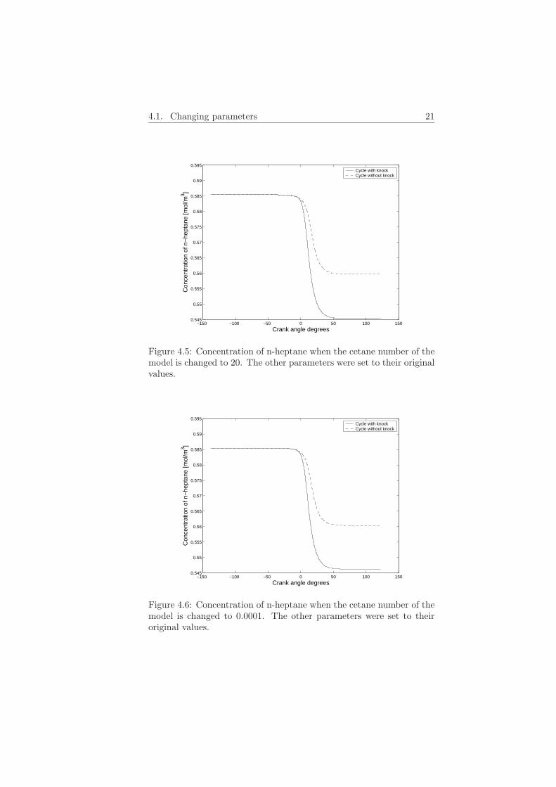
4.1. Changing parameters 21
−150 −100 −50 0 50 100 1500.545
0.55
0.555
0.56
0.565
0.57
0.575
0.58
0.585
0.59
0.595
Crank angle degrees
Con
cent
ratio
n of
n−
hept
ane
[mol
/m3 ]
Cycle with knockCycle without knock
Figure 4.5: Concentration of n-heptane when the cetane number of themodel is changed to 20. The other parameters were set to their originalvalues.
−150 −100 −50 0 50 100 1500.545
0.55
0.555
0.56
0.565
0.57
0.575
0.58
0.585
0.59
0.595
Crank angle degrees
Con
cent
ratio
n of
n−
hept
ane
[mol
/m3 ]
Cycle with knockCycle without knock
Figure 4.6: Concentration of n-heptane when the cetane number of themodel is changed to 0.0001. The other parameters were set to theiroriginal values.
22 Chapter 4. Evaluation of model
−150 −100 −50 0 50 100 1500.545
0.55
0.555
0.56
0.565
0.57
0.575
0.58
0.585
0.59
0.595
Crank angle degrees
Con
cent
ratio
n of
n−
hept
ane
[mol
/m3 ]
Cycle with knockCycle without knock
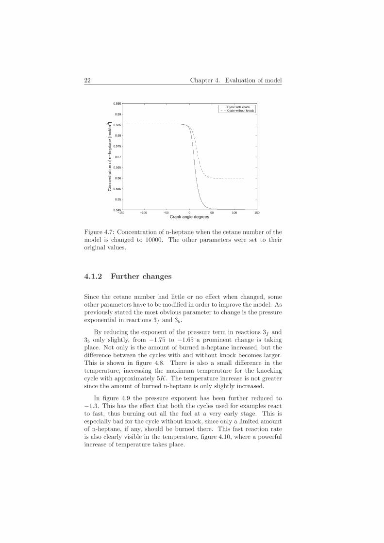
Figure 4.7: Concentration of n-heptane when the cetane number of themodel is changed to 10000. The other parameters were set to theiroriginal values.
4.1.2 Further changes
Since the cetane number had little or no effect when changed, someother parameters have to be modified in order to improve the model. Aspreviously stated the most obvious parameter to change is the pressureexponential in reactions 3f and 3b.
By reducing the exponent of the pressure term in reactions 3f and3b only slightly, from −1.75 to −1.65 a prominent change is takingplace. Not only is the amount of burned n-heptane increased, but thedifference between the cycles with and without knock becomes larger.This is shown in figure 4.8. There is also a small difference in thetemperature, increasing the maximum temperature for the knockingcycle with approximately 5K. The temperature increase is not greatersince the amount of burned n-heptane is only slightly increased.
In figure 4.9 the pressure exponent has been further reduced to−1.3. This has the effect that both the cycles used for examples reactto fast, thus burning out all the fuel at a very early stage. This isespecially bad for the cycle without knock, since only a limited amountof n-heptane, if any, should be burned there. This fast reaction rateis also clearly visible in the temperature, figure 4.10, where a powerfulincrease of temperature takes place.

4.1. Changing parameters 23
−150 −100 −50 0 50 100 1500.44
0.46
0.48
0.5
0.52
0.54
0.56
0.58
0.6
Crank angle degrees
Con
cent
ratio
n of
n−
hept
ane
[mol
/m3 ]
Cycle with knockCycle without knock
Figure 4.8: Concentration of n-heptane when the pressure exponent inreactions 3f and 3b has been reduced to −1.65, but all other parametersare set to their original values. Compared to the original model, a cleardifference is noticeable.
−150 −100 −50 0 50 100 1500
0.1
0.2
0.3
0.4
0.5
0.6
0.7
Crank angle degrees
Con
cent
ratio
n of
n−
hept
ane
[mol
/m3 ]
Cycle with knockCycle without knock
Figure 4.9: Concentration of n-heptane when the pressure exponent inreactions 3f and 3b has been further reduced, but all other parametersare set to their original values. As can be seen the reactions now takeplace to fast for both the cycles, since all fuel is burned out, even forthe cycle where knock does not occur.

24 Chapter 4. Evaluation of model
−150 −100 −50 0 50 100 150200
400
600
800
1000
1200
1400
1600
Crank angle degrees
Tem
pera
ture
[K]
Cycle with knockCycle without knock
Figure 4.10: Temperature when the pressure exponent in reactions 3f
and 3b has been further reduced. A clear self ignition can be spottedfor both the cycles, but should only be seen on one of th cycles.
4.1.3 Parameter optimization
To optimize the parameters of the model the program lsoptim [3] wasused. An error function with three parameters was created. The threeerror parameters was defined as follows:• Difference between end concentration of n-heptane and a control
concentration of n-heptane for the cycle without knock.• Difference between end concentration of n-heptane and a control
concentration for the cycle with knock.• Time of the knock in the knocking cycle.
To represent the fact that the cycle without knock might consumesome n-heptane, and the cycle with knock might not burn all n-heptane,the levels for the optimization was not set to the initial concentrationand zero. These levels are not in any way scientifically determined,they are only ad hoc. The levels are chosen only to loosen the demandson the cycles and are therefore set to 0.5 (compared to the initial con-centration 0.5856) and 0.1 (compared to 0).
The measured time when knock occurs in the knocking cycle wasdetermined with a function called knockfcn, and the time of knock inthe model was estimated in Matlab as:
min(diff(diff(C_1(:,9))./diff(t_1)));
where C_1(:,9) is the concentration of n-heptane and t_1 is the time.The reason for the min operator is because the concentration has a

4.1. Changing parameters 25
negative slant. Thus the function estimates the biggest difference be-tween two samples of the derivate to the n-heptane concentration. Thereason for this modeling of knock time is purely observational. Whenobserving a number of plots on the n-heptane concentration there isa similarity in that there is a break, or direction change, in the curveat the same time as the temperature rises clearly. This break in theconcentration curve is able to find using the command line above. Theproblem with this method is that if there is no break, or bend, in thecurve the estimation can place the time of the knock anywhere on thecurve. One other problem is that the method is only a variation ofdetecting knock on the pressure curve itself. This will be described insection 5.2. This can be avoided by using good starting points for theoptimization. There is also the factor that if there is no clear time forthe knock, the concentration of n-heptane has not been reduced veryfar, and thus creating a much larger error than the time. Therefore itis a usable method in this case.
4.1.4 Optimization method
As described in [3], the method used for optimization of the error func-tion can be described as a minimization of the following expression:
VN (θ) =12
N∑1
(yi − f(xi, θ))2 =N∑1
εi(θ)2 (4.1)
where N is the number of parameters in the model, θ the values ofthe parameters, yi the control values and xi a penalty vector. Theparameters, θ, must have an initial value, θ0, where the optimizationstarts.
The function lsoptim takes a function that creates the errors yi −f(xi, θ) as an argument as well as the initial values, θ0.
4.1.5 Optimization results
Running the optimization problem with all twelve parameters (the A, Eand n values, as well as the cetane number) as variables are a very timeconsuming process. Therefore a limitation on the number of variablesmust be made. To begin with, the optimization was run with thetwo parameters previously tested, to see if there was an optimum thatcould satisfy the demands. The parameters in the optimization werethe cetane number, CN, and the pressure exponent in equations 3.8and 3.9. The other parameters were set to the original conditions. Theinitial values of the two parameters were set to the original values,−1.75 and 5. To limit the time of the process the program was limited
26 Chapter 4. Evaluation of model
−150 −100 −50 0 50 100 150300
400
500
600
700
800
900
1000
1100
Crank angle degrees
Tem
pera
ture
[K]
Cycle with knockCycle without knock
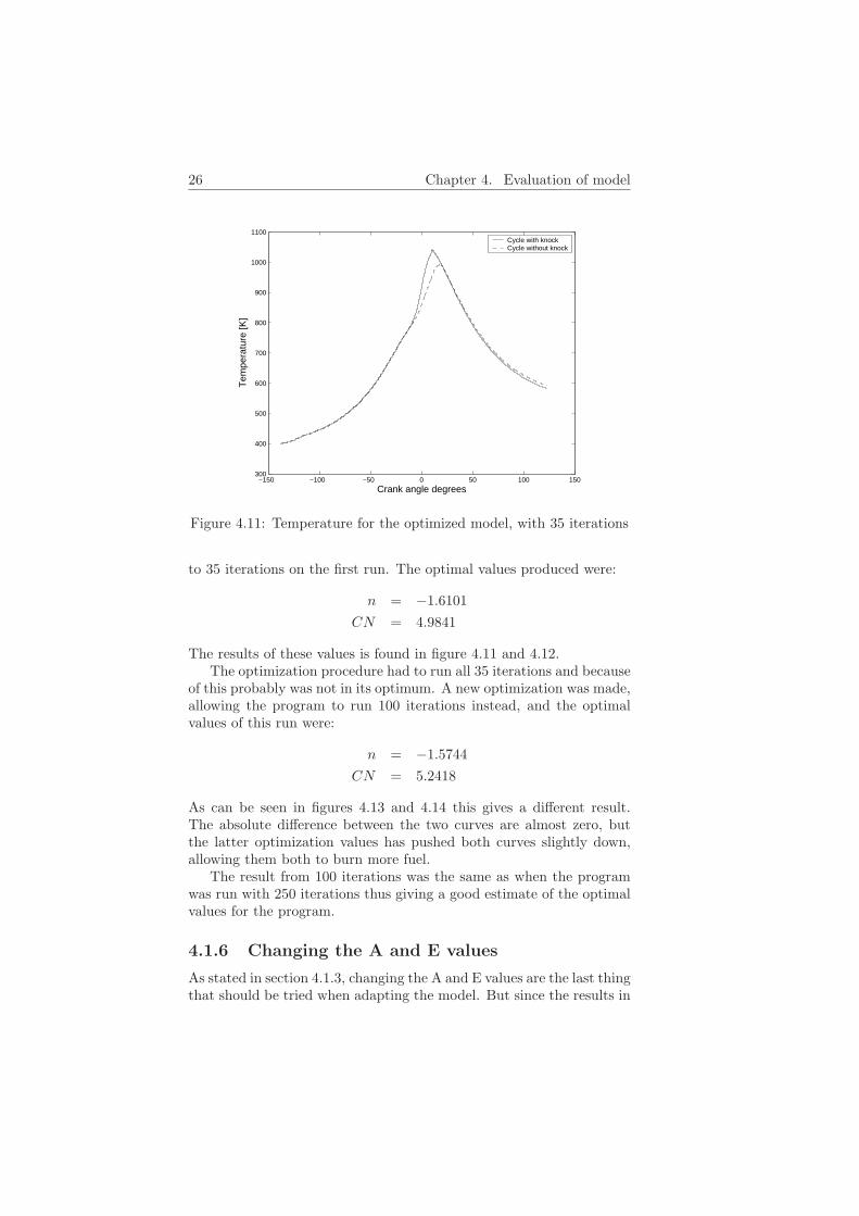
Figure 4.11: Temperature for the optimized model, with 35 iterations
to 35 iterations on the first run. The optimal values produced were:
n = −1.6101CN = 4.9841
The results of these values is found in figure 4.11 and 4.12.The optimization procedure had to run all 35 iterations and because
of this probably was not in its optimum. A new optimization was made,allowing the program to run 100 iterations instead, and the optimalvalues of this run were:
n = −1.5744CN = 5.2418
As can be seen in figures 4.13 and 4.14 this gives a different result.The absolute difference between the two curves are almost zero, butthe latter optimization values has pushed both curves slightly down,allowing them both to burn more fuel.
The result from 100 iterations was the same as when the programwas run with 250 iterations thus giving a good estimate of the optimalvalues for the program.
4.1.6 Changing the A and E values
As stated in section 4.1.3, changing the A and E values are the last thingthat should be tried when adapting the model. But since the results in

4.1. Changing parameters 27
−150 −100 −50 0 50 100 150
0.35
0.4
0.45
0.5
0.55
0.6
Crank angle degrees
Con
cent
ratio
n of
n−
hept
ane
[mol
/m3 ]
Cycle with knockCycle without knock
Figure 4.12: Concentration of n-heptane for the optimized model, with35 iterations
−150 −100 −50 0 50 100 150300
400
500
600
700
800
900
1000
1100
Crank angle degrees
Tem
pera
ture
[K]
Cycle with knockCycle without knock
Figure 4.13: Temperature for the optimized model, with 100 iterations

28 Chapter 4. Evaluation of model
−150 −100 −50 0 50 100 1500.25
0.3
0.35
0.4
0.45
0.5
0.55
0.6
0.65
Crank angle degrees
Con
cent
ratio
n of
n−
hept
ane
[mol
/m3 ]
Cycle with knockCycle without knock
Figure 4.14: Concentration of n-heptane for the optimized model, with100 iterations
the previous sections are not good enough, the method should at leastbe evaluated. This could be done using the same optimization methodas above, but instead of changing the n and CN values some of the Aand/or E values should be parameters to the optimization model. Thisis however not a satisfactory way of dealing with the problem, sincethe model contains a large amount of local minima that will stop theoptimization process. This is a problem since the model requires largechanges in the A and E values to make any difference, and thereforethe optimization process will not be effective enough.
The other way of adapting the A and E values is by making a lot ofruns, manually changing the values, learning by trial and error methodwhich values that effect the model. But before doing this a plan has tobe made on what to change. To do this there consideration to all thefactors must be made.
The primary goal of the model is to detect knock. Therefore awider gap between the n-heptane concentrations of the cycles with andwithout knock must be created. Since previous tests have shown thatchanging the parameter A4 (which is the same as changing the cetanenumber) does not give any large effect on the output, this should beconsidered stationary. Furthermore, when studying plots of the differ-ent interim species, especially HO2C7H13O and CH3, the conclusioncan be made that most of the fuel is burned by reactions 3f , 3b and4. It is also apparent that the reactions 1 and 2 do not have that bigeffect on the system and therefore these should be made faster.

4.1. Changing parameters 29
−150 −100 −50 0 50 100 150300
400
500
600
700
800
900
1000
1100
Crank angle degrees
Tem
pera
ture
[K]
Cycle with knockCycle without knock
Figure 4.15: Temperature of the adapted model, where E1 = 156 ∗ 103
and A1 = 4.5 ∗ 1010
Several tries with different values were made, with both small andbig increases of the values and after a while it became apparent thatthe factors that had the most effect on the system were A1 and E1. Asmall increase in E1 with only 4% and a bigger change in A1, with afactor 50. Attempts to change the other parameters were made, butthe changes in the result were very small, even for very large changesin the parameters. Therefore these parameters were not changed, sinceit would take the model further away from the original model. Theresults from this model are shown in figures 4.15 and 4.16.
The optimization program described earlier was tested on this adaptedmodel to find the optimal cetane number and pressure exponent.

30 Chapter 4. Evaluation of model
−150 −100 −50 0 50 100 1500.25
0.3
0.35
0.4
0.45
0.5
0.55
0.6
0.65
Crank angle degrees
Con
cent
ratio
n of
n−
hept
ane
[mol
/m3 ]
Cycle with knockCycle without knock
Figure 4.16: Concentration of n-heptane of the adapted model, whereE1 = 156 ∗ 103 and A1 = 4.5 ∗ 1010

Chapter 5
Analysis
Since the original model gives a clear, if not big, difference betweencycles that knock and cycles that do not, it was finally chosen as themodel to use. The main reason for this is the fact that in order to get themodel better, a big change has to be made to some of the parameters,thus taking the model very far from it’s original state. So instead ofmarginally changing the parameters with no or little effect, the originalmodel is kept. The model should be able to do two things. First itshould be able to detect if knock occurs (section 5.1), and second todecide at what time it occurs (section 5.2). In section 5.3 the model iscompared to another model for determining knock to see if this is anacceptable method.
5.1 Detection
The detection is solved by a check on the concentration of n-heptaneat the end of the cycle. If this concentration is below a certain valuethe cycle knocks. The detection level was decided by looking at sev-eral different cycles, figures 5.1, 5.2 and 5.3 show some of these cycles.The level was then set to a values between the cycles with and withoutknock. The value chosen was a linear function depending on the com-pression ratio, since the levels of ignited n-heptane was very differentfor different rc. Thus the level was set to 0.427 + 0.01rc mol/m3. Anycycle that has a concentration of n-heptane equal to or higher than thisvalues at the end of the cycle is considered not to have knocked. Cycleswith values below this level have knocked.
This method is however not bulletproof. In the border betweencycles that knocks and cycles that don’t, some cycles will end up on thewrong side of the line. These cycles are the ones with a very marginalknock and since this is barely noticeable the model is set so that all
31

32 Chapter 5. Analysis
−150 −100 −50 0 50 100 150
0.55
0.56
0.57
0.58
0.59
Crank angle degrees
Con
cent
ratio
n of
n−
hept
ane
[mol
/m3 ]
Cycle without knockCycle with knockCycle without knockCycle with knock
Figure 5.1: Cycles used to validate the model and to decide where thelevel for knock should be. The dotted vertical line is the limit for knock.θi = 18◦BTDC, rc = 12.
−150 −100 −50 0 50 100 150
0.55
0.56
0.57
0.58
0.59
Crank angle degrees
Con
cent
ratio
n of
n−
hept
ane
[mol
/m3 ]
Cycle witout knockCycle with knockCycle with knockCycle with knock
Figure 5.2: Cycles used to validate the model and to decide where thelevel for knock should be. The dotted vertical line is the limit for knock.θi = 16◦BTDC, rc = 13.

5.2. Time of knock 33
−150 −100 −50 0 50 100 1500.53
0.54
0.55
0.56
0.57
0.58
0.59
0.6
Crank angle degrees
Con
cent
ratio
n of
n−
hept
ane
[mol
/m3 ]
Cycle with knockCycle with knockCycle with knockCycle with knock
Figure 5.3: Cycles used to validate the model and to decide where thelevel for knock should be. The dotted vertical line is the limit for knock.As can be seen, one cycle with knock is above the dotted line and willnot be detected by the program. θi = 22◦BTDC, rc = 11.
of these are treated as if they don’t knock. An example of this is thecycle in figure 5.3 with the least amount of burned n-heptane. As canbe seen in figure 5.4 the knock in the cycle is small and the oscillationsbarely noticeable.
Even though the method for detecting knock is not perfect, it has ahigh level of reliability. Most of the undetected cycles are on the limitof being knock and are therefore hard to detect with any method. Thedifference between these cycles and the ones where the only oscillationsare interference from the sensors or other things is very small. Thereforethis limitation does not affect the general system all that much and canbe accepted as a part of the model.
5.2 Time of knock
To determine the time of knock is rather difficult using this model.The best way is to look at the concentration of n-heptane. Whenknock occurs, the n-heptane will start to burn faster. The derivate ofthe n-heptane concentration therefore decreases at the same time asthe knock starts. This decrease should be easy to find if the knockwas obvious, but in this model it is harder. It is found by lookingfor the biggest difference between two samples of the derivate of theconcentration of n-heptane. In Matlab it looks like this:
34 Chapter 5. Analysis
5 10 15 20 25
4
4.2
4.4
4.6
4.8
5
5.2
5.4
5.6
5.8
6x 10
6
Crank angle degrees
Pre
ssur
e [P
a]
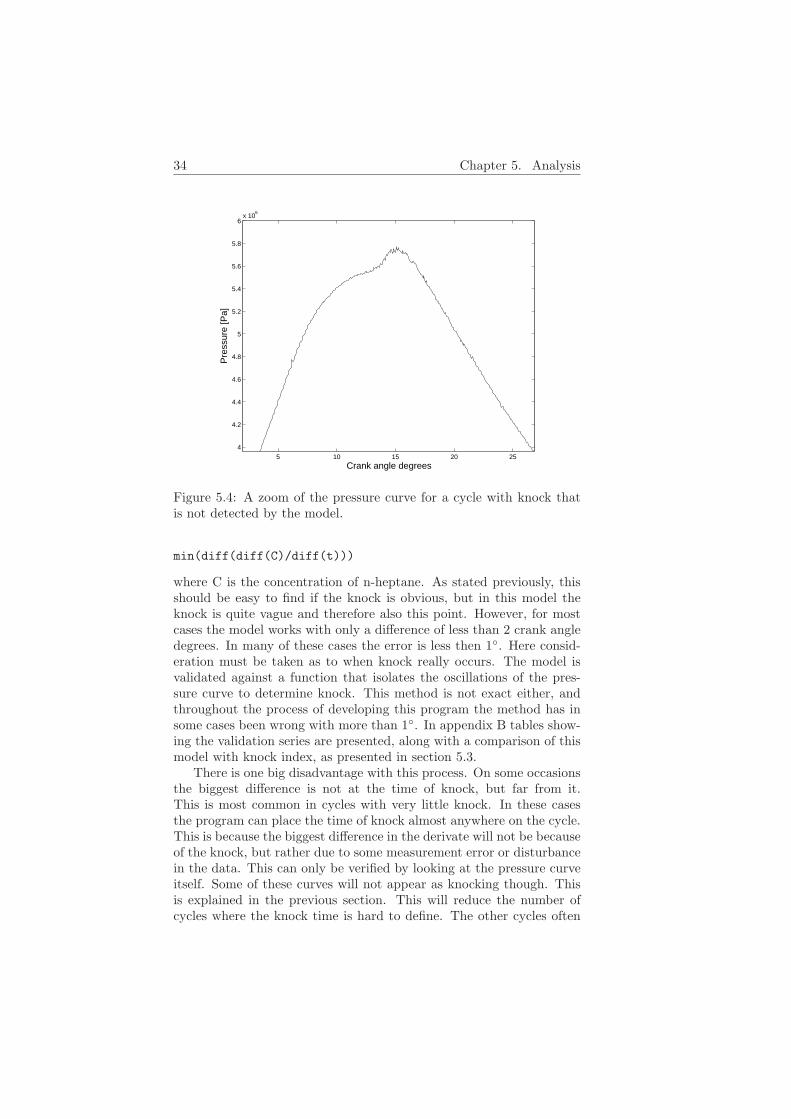
Figure 5.4: A zoom of the pressure curve for a cycle with knock thatis not detected by the model.
min(diff(diff(C)/diff(t)))
where C is the concentration of n-heptane. As stated previously, thisshould be easy to find if the knock is obvious, but in this model theknock is quite vague and therefore also this point. However, for mostcases the model works with only a difference of less than 2 crank angledegrees. In many of these cases the error is less then 1◦. Here consid-eration must be taken as to when knock really occurs. The model isvalidated against a function that isolates the oscillations of the pres-sure curve to determine knock. This method is not exact either, andthroughout the process of developing this program the method has insome cases been wrong with more than 1◦. In appendix B tables show-ing the validation series are presented, along with a comparison of thismodel with knock index, as presented in section 5.3.
There is one big disadvantage with this process. On some occasionsthe biggest difference is not at the time of knock, but far from it.This is most common in cycles with very little knock. In these casesthe program can place the time of knock almost anywhere on the cycle.This is because the biggest difference in the derivate will not be becauseof the knock, but rather due to some measurement error or disturbancein the data. This can only be verified by looking at the pressure curveitself. Some of these curves will not appear as knocking though. Thisis explained in the previous section. This will reduce the number ofcycles where the knock time is hard to define. The other cycles often
5.3. Knock index 35
−150 −100 −50 0 50 100 1500
1
2
3
4
5
6
7x 10
6
Crank angle degrees
Pre
ssur
e [P
a]
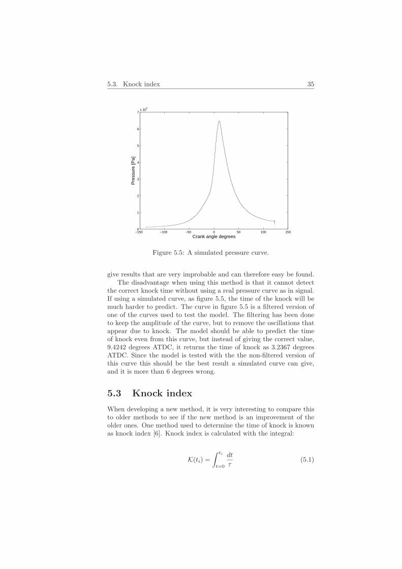
Figure 5.5: A simulated pressure curve.
give results that are very improbable and can therefore easy be found.The disadvantage when using this method is that it cannot detect
the correct knock time without using a real pressure curve as in signal.If using a simulated curve, as figure 5.5, the time of the knock will bemuch harder to predict. The curve in figure 5.5 is a filtered version ofone of the curves used to test the model. The filtering has been doneto keep the amplitude of the curve, but to remove the oscillations thatappear due to knock. The model should be able to predict the timeof knock even from this curve, but instead of giving the correct value,9.4242 degrees ATDC, it returns the time of knock as 3.2367 degreesATDC. Since the model is tested with the the non-filtered version ofthis curve this should be the best result a simulated curve can give,and it is more than 6 degrees wrong.
5.3 Knock index
When developing a new method, it is very interesting to compare thisto older methods to see if the new method is an improvement of theolder ones. One method used to determine the time of knock is knownas knock index [6]. Knock index is calculated with the integral:
K(ti) =∫ ti
t=0
dt
τ(5.1)
36 Chapter 5. Analysis
where
τ = Ap−ne(B/T ) (5.2)
Knock is expected to occur when K(ti) = 1. As can be seen theexpression for calculation of τ is very like the modified Arrhenius ex-pression used in section 3.1.1.
Sometimes K(ti) = 1 very late in the cycle, when it is not very likelythat it will knock, since it is not enough fuel left. According to Soltic[12], there is an upper limit to how much of the fuel can be burnt andstill cause knock. This is because the temperature of the outer layersof the fuel never can rise so high as to cause knock since the coolingeffect of the cylinder prevents this. Soltic sets this limit to 75% of thefuel. In appendix B several series of validation data can be found. Thedata compares the knock index with the model used in this report andverifies both models against the observed time of knock.
Chapter 6
Conclusions
The method studied in this report has proven to be fairly reliable whendetecting knock. It has, however, difficulties detecting the time of theknock, especially when running the model with a simulated pressurecurve. Even when running the program with a real pressure curve,some of the estimations for the knock time is very wrong, sometimesas much as 8 or 10 degrees. The results can be summed up as follows:+ Predicts if knock occurs with good reliability+ Can predict time fairly well when using a real pressure curve- Can not predict time of knock when using a simulated pres-
sure curve- Some estimations of knock time are very wrong, up to 8 or
10 degrees- Hard to detect knock in the border between knock and no
knockOf these, the last point is not that serious. The border between
knock and no knock is very vague and there can be no expectations ona model of this kind to be able to simulate that with good accuracy.The real big errors fall into this category too. Since there is no clearknock on the pressure curve, there will be no clear knock time either.This normally occurs when the knock is very small.
The other two negative factors are, however, a big disadvantage tothe model. The simulation time is much longer then when running aknock index simulation. This could be made faster, but not withoutreducing the accuracy of the model. The big danger by doing this isthat there is a risk of getting negative concentrations, and if this occursthe model will give a really bad result. Compared to knock index thebiggest disadvantage is that you cannot use a simulated pressure curveas input to the model. It will be able to detect if knock occurs, but notwhen, at least not with any accuracy.
On the total, this model is not an improvement over knock index.
37

38 Chapter 6. Conclusions
The only thing that it might do better is to determine whether knockhas occurred or not, but even this is not clear. The small advantageswith this model is not enough to use it instead of knock index, sincethe disadvantages with the model are too great.
6.1 Future work
As shown, the model used here was not sufficient to model knock iniso-octane combustion. This does not mean that the model is unus-able. Further evaluation of the model when using n-heptane, or diesel,fuel could be tried. As shown above, this will probably give a moresatisfying result.
To be able to model iso-octane combustion, a more thorough modelmight have to be used. At least, the model should be based on iso-octane, and not, as in this case, an adaption of an n-heptane model. Itcould be used to adapt the existing model, by adding other substancesand reactions. If using the same temperature model, this is easy to do.The program in its current state is however not very usable

References
[1] Per Amneus. Homogeneous Ignition - Chemical Kinetic Studies forIC-Engine Applications. PhD thesis, Department of CombustionPhysics, Lund Institute of Technology, Lund, Sweden, 2002.
[2] L. Eriksson and P. Andersson. Calculation of chemical equlib-rium. Technical report, Department of Electrical Engineering,Linkopings Universitet, Linkoping, Sweden, 2002.
[3] Lars Eriksson. Minimal manual to lsoptim. Department of Electri-cal Engineering, Linkopings Universitet, Linkoping, Sweden, 1991.
[4] Lars Eriksson. Documentation for the CHemical Equilibrium Pro-gram Package, CHEPP. Department of Electrical Engineering,Linkopings Universitet, Linkoping, Sweden, 2000.
[5] Irvin Glassman. Combustion. Academic Press, Inc., San Diego,U.S.A., 3 edition, 1996.
[6] John B. Heywood. Internal Combustion Engine Fundamentals.McGraw-Hill Book Co., international edition, 1988.
[7] Lawrence Livermore National Laboratory. Detailed model ofn-heptane combustion. internet, June 2003. http://www-cms.llnl.gov/combustion/combustion2.html#n-C7H16.
[8] B.J. McBride and S. Gordon. Computer program for calcu-lating and fitting thermodynamic functions. Technical ReportNASA-RP-1271, NASA, Lewis Research Center, Cleveland, U.S.A,November 1992.
[9] Ulf Christian Muller. Reduzierte Reaktionsmechanismen fur dieZundung von n-Heptan und iso-Oktan unter motorrelevanten Be-dingungen. PhD thesis, RWTH, Aachen, Aachen, Germany, 1993.
[10] L. Nielsen and L. Eriksson. Course material, vehicular systems.Linkoping, Sweden, 2001. Linkopings Universitet, Sweden.
39
40 References
[11] D. Nilsson, T. Løvas, P. Amneus, and F. Mauss. Reduction ofcomplex fuel chemistry for simulation of combustion in an hcciengine. VDI Berichte, (1492):511–516, 1999.
[12] Patrik Soltic. Part-Load Optimized SI Engine Systems. PhD thesis,Swiss Federal Institute of Technology, Zurich, Switzerland, 2000.
[13] H. Soyhan, P. Amneus, F. Mauss, and C. Sorusbay. A skeletalmechanism for the oxidation of iso-octane and n-heptane validatedunder engine knock conditions. Technical Report 1999-01-3484,SAE Technical Paper Series, Toronto, Canada, 1999.
[14] Charles Fayette Taylor. The Internal-Combustion Engine in The-ory and Practice. The MIT Press, Camebridge, U.S.A., 7 edition,1985.

Notation
Symbols used in the report.
Variables and parameters
t TimeT Temperaturep PressureA Constant of the Ahrenius functionn Exponent of the Ahrenius functionE Energy barrier of the Ahrenius functionR Rydbergs constantkf Transfer rateK Chemical equilibrium concentrationM Molemasscp Specific heath Enthalpyx Fractionω Total reaction ratecp Specific heatν Number of reacting molecules
Aw Wall area of cylinderV Volumerc Compression ratio
Abbreviations
BDC Bottom Dead CenterTDC Top Dead CenterCN Cetane Number
Operators
[A] Concentration of AA Mole fraction of A
41

42 Notation
Subscripts
u Unburnedw Wall of cylinder
Appendix A
Manual for the program
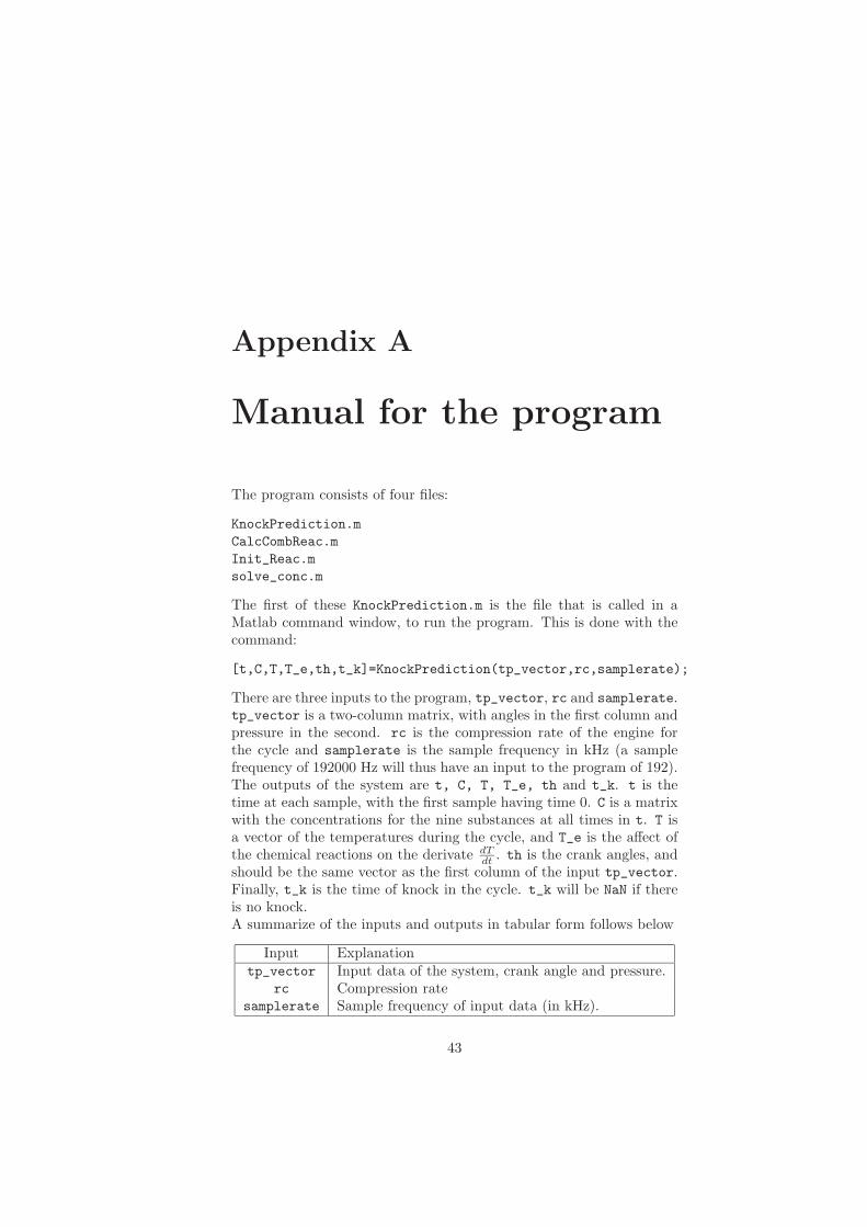
The program consists of four files:
KnockPrediction.mCalcCombReac.mInit_Reac.msolve_conc.m
The first of these KnockPrediction.m is the file that is called in aMatlab command window, to run the program. This is done with thecommand:
[t,C,T,T_e,th,t_k]=KnockPrediction(tp_vector,rc,samplerate);
There are three inputs to the program, tp_vector, rc and samplerate.tp_vector is a two-column matrix, with angles in the first column andpressure in the second. rc is the compression rate of the engine forthe cycle and samplerate is the sample frequency in kHz (a samplefrequency of 192000 Hz will thus have an input to the program of 192).The outputs of the system are t, C, T, T_e, th and t_k. t is thetime at each sample, with the first sample having time 0. C is a matrixwith the concentrations for the nine substances at all times in t. T isa vector of the temperatures during the cycle, and T_e is the affect ofthe chemical reactions on the derivate dT
dt . th is the crank angles, andshould be the same vector as the first column of the input tp_vector.Finally, t_k is the time of knock in the cycle. t_k will be NaN if thereis no knock.A summarize of the inputs and outputs in tabular form follows below
Input Explanationtp_vector Input data of the system, crank angle and pressure.
rc Compression ratesamplerate Sample frequency of input data (in kHz).
43

44 Appendix A. Manual for the program
Output Explanationt TimeC Concentrations of the reacting substancesT Temperature.T_e Affect of chemical reactions on the temperature.th Crank anglet_k Time of knock (Nan if no knock)
When running the program, an external window will open for Chepp.This will be done in the lowest available figure number of Matlab. It isnecessary to have a Chepp version that can handle all the substances inthe reactions, or the program will not work. The substances specificallyadded for this program is C7H16 and HO2C7H13O.

Appendix B
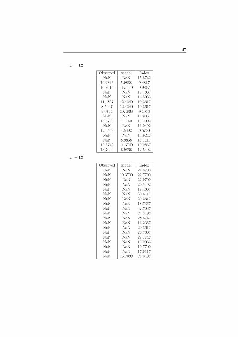
Validation data
The results from the validation of the program is shown below. Thefirst column, observed, is the observed time of knock from a pressurecurve. The second column, model, is the result from the model de-scribed in this report and the third column, index, is the result whenusing knock index as described in section 5.3. All values are crank angledegrees an NaN (Not a Number) means no knock has been detected.NaN will never appear in the knock index column since knock indexcan not decide whether knock has occurred or not, only when it hasoccurred.
45

46 Appendix B. Validation data
rc = 10
Observed model Index0.8617 3.1117 1.6117-1.8836 -0.2633 -1.20081.3617 NaN 1.79921.0492 NaN 0.5492NaN NaN 0.6117NaN NaN 2.5492
-1.0133 NaN -1.13832.5492 NaN 3.1117NaN NaN 1.9242NaN NaN 0.7992NaN NaN 2.3617
5.7992 NaN 4.6117-2.0758 -1.9508 -2.4508NaN NaN -0.7008NaN NaN 2.1117NaN NaN -0.1383
0.3617 NaN 0.6117-0.0758 NaN -0.3883NaN NaN 2.1117
1.1742 NaN 0.2367
rc = 11
Observed model IndexNan NaN 13.6325
6.9200 NaN 5.4825NaN NaN 9.8325
4.6700 5.9200 4.8575NaN NaN 10.4200NaN NaN 8.2325
12.6700 NaN 11.0450NaN NaN 9.6325
9.4325 NaN 7.1700NaN NaN 10.6700
4.8575 NaN 4.1658NaN NaN 5.9825NaN 15.4825 7.4200NaN 4.8575 11.7950NaN NaN 7.5450NaN NaN 6.6700NaN NaN 13.9658NaN NaN 7.4200NaN NaN 6.6700
47
rc = 12
Observed model IndexNaN NaN 15.6742
10.2846 5.9868 9.486710.8616 11.1119 9.9867NaN NaN 17.7367NaN NaN 16.5033
11.4867 12.4240 10.36178.5697 12.4240 10.36179.6744 10.4868 9.1033NaN NaN 12.9867
13.3700 7.1740 11.2992NaN NaN 16.0492
12.0493 4.5492 9.5700NaN NaN 14.9242NaN 8.9868 12.1117
10.6742 11.6740 10.986713.7699 6.9866 12.5492
rc = 13
Observed model IndexNaN NaN 22.3700NaN 19.3700 22.7700NaN NaN 22.9700NaN NaN 20.5492NaN NaN 19.4367NaN NaN 30.6117NaN NaN 20.3617NaN NaN 18.7367NaN NaN 32.7037NaN NaN 21.5492NaN NaN 28.6742NaN NaN 16.2367NaN NaN 20.3617NaN NaN 20.7367NaN NaN 29.1742NaN NaN 19.9033NaN NaN 19.7700NaN NaN 17.6117NaN 15.7033 22.0492
Upphovsrätt
Detta dokument hålls tillgängligt på Internet – eller dess framtida ersättare –under en längre tid från publiceringsdatum under förutsättning att inga extra-ordinära omständigheter uppstår.
Tillgång till dokumentet innebär tillstånd för var och en att läsa, ladda ner,skriva ut enstaka kopior för enskilt bruk och att använda det oförändrat förickekommersiell forskning och för undervisning. Överföring av upphovsrättenvid en senare tidpunkt kan inte upphäva detta tillstånd. All annan användning avdokumentet kräver upphovsmannens medgivande. För att garantera äktheten,säkerheten och tillgängligheten finns det lösningar av teknisk och administrativart.
Upphovsmannens ideella rätt innefattar rätt att bli nämnd som upphovsman iden omfattning som god sed kräver vid användning av dokumentet på ovanbeskrivna sätt samt skydd mot att dokumentet ändras eller presenteras i sådanform eller i sådant sammanhang som är kränkande för upphovsmannens litteräraeller konstnärliga anseende eller egenart.
För ytterligare information om Linköping University Electronic Press seförlagets hemsida http://www.ep.liu.se/
Copyright
The publishers will keep this document online on the Internet - or its possiblereplacement - for a considerable time from the date of publication barringexceptional circumstances.
The online availability of the document implies a permanent permission foranyone to read, to download, to print out single copies for your own use and touse it unchanged for any non-commercial research and educational purpose.Subsequent transfers of copyright cannot revoke this permission. All other usesof the document are conditional on the consent of the copyright owner. Thepublisher has taken technical and administrative measures to assure authenticity,security and accessibility.
According to intellectual property law the author has the right to bementioned when his/her work is accessed as described above and to be protectedagainst infringement.
For additional information about the Linköping University Electronic Pressand its procedures for publication and for assurance of document integrity,please refer to its WWW home page: http://www.ep.liu.se/
© [2003, Tomas Lidholm]