kohler, shane jerome

Non-Linear Eects in Quantum

Electrodynamics

by

Kohler, Shane Jerome

Thesis presented in partial fulllment of the

requirements for the degree of Masters of Science

at

Stellenbosch University

Department of Physics

Faculty of Science

Supervisor: Prof Cesareo Dominguez

Co-supervisor: Prof Heinrich Schwoerer

Date: December 2010

Declaration

By Submitting this thesis electronically, I declare that the entirety of the workcontained therein is my own, original work, that I am the owner of the copy-right thereof and that I have not previously in its entirety or in part submittedit for obtaining any qualication.

Date: 26 November 2010

Copyright c© 2010 Stellenbosch University

All rights reserved

Stellenbosch University http://scholar.sun.ac.za

Abstract

The Euler-Heisenberg Lagrangian is used to derive equations for the electricand magnetic elds (~E(~x) and ~B(~x) respectively) induced by the interactionof external quasistatic electric/magnetic elds and the the elds produced byclassical charges and currents.

~E(~x) =ζ

4πε20~∇x∫

d3y

|~x− ~y|~∇y ·

8FM ~DM +

14

cGM ~HM

~B(~x) =ζ

4πε20c~∇x ×

∫d3y

|~x− ~y|~∇y ×

−8

cFM ~HM + 14GM ~DM

In particular, the cases of the uniformly charged spherical shell in the presenceof a external magnetic eld and of the spherical magnetic dipole in the presenceof an external electric eld were investigated. It was found that the externalmagnetic eld induced a magnetic dipole moment (~m) in the uniformly chargedshell.

~m =c2ζ

6πε20

Q2

R~B0

The external electric eld had a similar eect on the spherical magnetic dipolewhere it induced an electric dipole moment (~pψ).

~pψ =ζµ0m

2E0

10πε0R3

[36~E0

E0− 49

( ~E0 · ex)exE0

]

These results are quite surprising since they predict eects which were notexpected. Some experiments to observe these induced elds will be discussedbriey.


Opsomming

Die Euler-Heisenberg Lagrangian word gebruik om vergelykings vir die elek-triese (~E(~x)) en magnetiese ( ~B(~x)) velde af te lei. Hierdie velde onstaan weensdie interaksie tussen eksterne elektriese/magnetiese velde en die velde vanklassieke ladings en strome.

~E(~x) =ζ

4πε20~∇x∫

d3y

|~x− ~y|~∇y ·

8FM ~DM +

14

cGM ~HM

~B(~x) =ζ

4πε20c~∇x ×

∫d3y

|~x− ~y|~∇y ×

−8

cFM ~HM + 14GM ~DM

Ons ondersoek die geval waar 'n uniform gelaaide sferiese skil teenwoordig isin 'n eksterne magnetiese veld en waar 'n sferiese magnetiese dipool (~m) in 'neksterne elektriese veld teenwoordig is. Ons vind dat die eksterne elektrieseveld 'n magnetiese dipoolmoment in die uniform gelaaide skil geïnduseer.

~m =c2ζ

6πε20

Q2

R~B0

Die eksterne elektriese veld het 'n soortgelyk eek gehad op die sferiese mag-netiese dipool waar dit 'n elektriese dipool (~pψ) veroorsaak het.

~pψ =ζµ0m

2E0

10πε0R3

[36~E0

E0− 49

( ~E0 · ex)exE0

]

Hierdie resultate is nogal verbasend aangesien hulle gevolge voorspel wat nieverwag was nie. Sekere eksperimente wat hierdie geïnduseerde velde waarneemis kortliks bespreek.


Acknowledgements

I would like to thank everyone who made it possible from me fulll my MScespecially:

• Prof. C. A. Dominguez

• Prof. G. Hillhouse

• Prof. H. Schwoerer

• all those who attended the Non-Linear QED workshop in September 2009

• National Research Foundation

I would also like to extend my gratitude to those who kept me going thoughmy studies especially:

• my family

• my friends

• God

The nancial assistance of the National Research Foundation (NRF) towardsthis research is hereby acknowledged. Opinions expressed and conclusions

arrived at, are those of the author and are not necessarily to be attributed tothe National Research Foundation.


Contents

Contents i

List of Figures ii

1 Introduction 1

1.1 Classical Electrodynamics . . . . . . . . . . . . . . . . . . . . . 11.2 Quantum Electrodynamics . . . . . . . . . . . . . . . . . . . . . 21.3 Non-Linear Quantum Electrodynamics . . . . . . . . . . . . . . 31.4 Euler-Heisenberg Lagrangian . . . . . . . . . . . . . . . . . . . 3

2 Theory 6

2.1 Derivation of the Induced Electric and Magnetic Field Equations 62.1.1 Dening the Auxiliary Fields ~D and ~H . . . . . . . . . . 62.1.2 Expressions for ~E and ~B . . . . . . . . . . . . . . . . . . 72.1.3 General Solutions using Maxwell's Equations . . . . . . 92.1.4 Obtaining the Induced Fields ~E and ~B . . . . . . . . . . 10

2.2 Summary and Discussion . . . . . . . . . . . . . . . . . . . . . 12

3 Investigating the Induced Fields 13

3.1 Charged Shell in a Quasi-static Magnetic Field . . . . . . . . . 133.1.1 The Situation . . . . . . . . . . . . . . . . . . . . . . . . 133.1.2 Calculating ~E(~x) . . . . . . . . . . . . . . . . . . . . . . 14

3.1.3 Calculating ~B(~x) . . . . . . . . . . . . . . . . . . . . . . 173.1.4 Summary and Discussion . . . . . . . . . . . . . . . . . 18

3.2 Spherical Magnetic Dipole in a Quasi-static Electric Field . . . 193.2.1 The Situation . . . . . . . . . . . . . . . . . . . . . . . . 193.2.2 Calculating ~E(~x) . . . . . . . . . . . . . . . . . . . . . . 20

3.2.3 Calculating ~B(~x) . . . . . . . . . . . . . . . . . . . . . . 233.2.4 Summary and Discussion . . . . . . . . . . . . . . . . . 27

4 Experimental Observability and Conclusion 29

4.1 Experimental Observability . . . . . . . . . . . . . . . . . . . . 294.1.1 Charged Spherical Shell in a Quasi-static Magnetic Field 294.1.2 Spherical Magnetic Dipole in a Quasi-static Electric Field 30

4.2 Outlook . . . . . . . . . . . . . . . . . . . . . . . . . . . . . . . 324.3 Conclusion . . . . . . . . . . . . . . . . . . . . . . . . . . . . . 32

Bibliography 34

i


List of Figures

1.1 Diagrammatic representation of the one-loop contribution to thevacuum polarization . . . . . . . . . . . . . . . . . . . . . . . . . . 2

1.2 Diagrammatic representation of the one-loop eective action in thepresence of a background electromagnetic eld . . . . . . . . . . . 4

3.1 A charged shell in an external magnetic eld . . . . . . . . . . . . 133.2 A spherical magnetic moment in an external electric eld . . . . . 19

4.1 The induced electric dipole moment in relation to the external elec-tric eld . . . . . . . . . . . . . . . . . . . . . . . . . . . . . . . . . 31

ii


Chapter 1

Introduction

1.1 Classical Electrodynamics

Light is one of the most fascinating subjects in physics. It has been studied andcontemplated since the earliest days. However, mankind's understanding of thenature of light has been greatly increased during the last few centuries. JamesMaxwell study of light in the 1860's and 1870's led to the general acceptanceof the idea that light is a form of electromagnetic radiation.

During his studies, Maxwell was able to compile a list of equations to cal-culate electric and magnetic elds. This list consisted of four equations whichbecame known collectively as Maxwell's equations [7]:

~∇ · ~E =1

ε0ρ ~∇× ~E +

∂ ~B

∂t= 0

~∇ · ~B = 0 ~∇× ~B − µ0ε0∂ ~E

∂t= µ0

~J

These equations form the basis for classical electrodynamics.

Electrodynamics, as the name suggests, deals with electric and magnetic eldswhich change with time. This is easily seen in the equations above where ~∇× ~Eand ~∇× ~B depend on ∂ ~B

∂t and ∂ ~E∂t respectively; or where the time dependence is

contained in the source terms ρ and ~J . Maxwell's equations take on a slightlydierent form when they describe electric and magnetic elds within matter:

~∇ · ~D = ρf ~∇× ~E = −∂~B

∂t

~∇ · ~B = 0 ~∇× ~H = ~Jf +∂ ~D

∂t

The above equations make use of the electric displacement eld ~D and themagnetization eld ~H. These two elds give information regarding the polar-ization and magnetization of the medium in which the electric and magneticelds are found. In general, it is possible to dene ~D and ~H in terms of the

1


CHAPTER 1. INTRODUCTION 2

electric and magnetic polarization vectors, ~P and ~M respectively:

~D = ε0 ~E + ~P ~H =1

µ0

~B − ~M

According to classical electrodynamics, the vacuum does not consist of anyparticles. This automatically implies a linear relation between ~D and ~E as wellas a linear relation between ~H and ~B since the lack of charged particles meansthat the medium, in this case the vacuum, will have no polarization.

1.2 Quantum Electrodynamics

The theory of quantum electrodynamics (QED) was developed using quantumeld theory and the theory of special relativity to describe the electric andmagnetic interactions between fundamental particles. Contributions to QEDwere made by Richard Feynman, Julian Schwinger and Sin-Itiro Tomonaga forwhich they were awarded the 1965 Nobel Prize in Physics.

This electromagnetic interaction is expressed as an exchange of photonsbetween the particles. Where the total interaction is the combination of all thepossible exchanges between the particles. Examples of the types of possibleinteractions include:

• the exchange of one or more photons

• an emitted photon splitting into a particle and its anti-particle beforerecombining into a photon

A graphical way of expressing this interaction was developed by Feynman.This graphical representation became know as Feynman Diagrams where eachdiagram represents a term in the perturbation expansion of the lagrangiandensity.

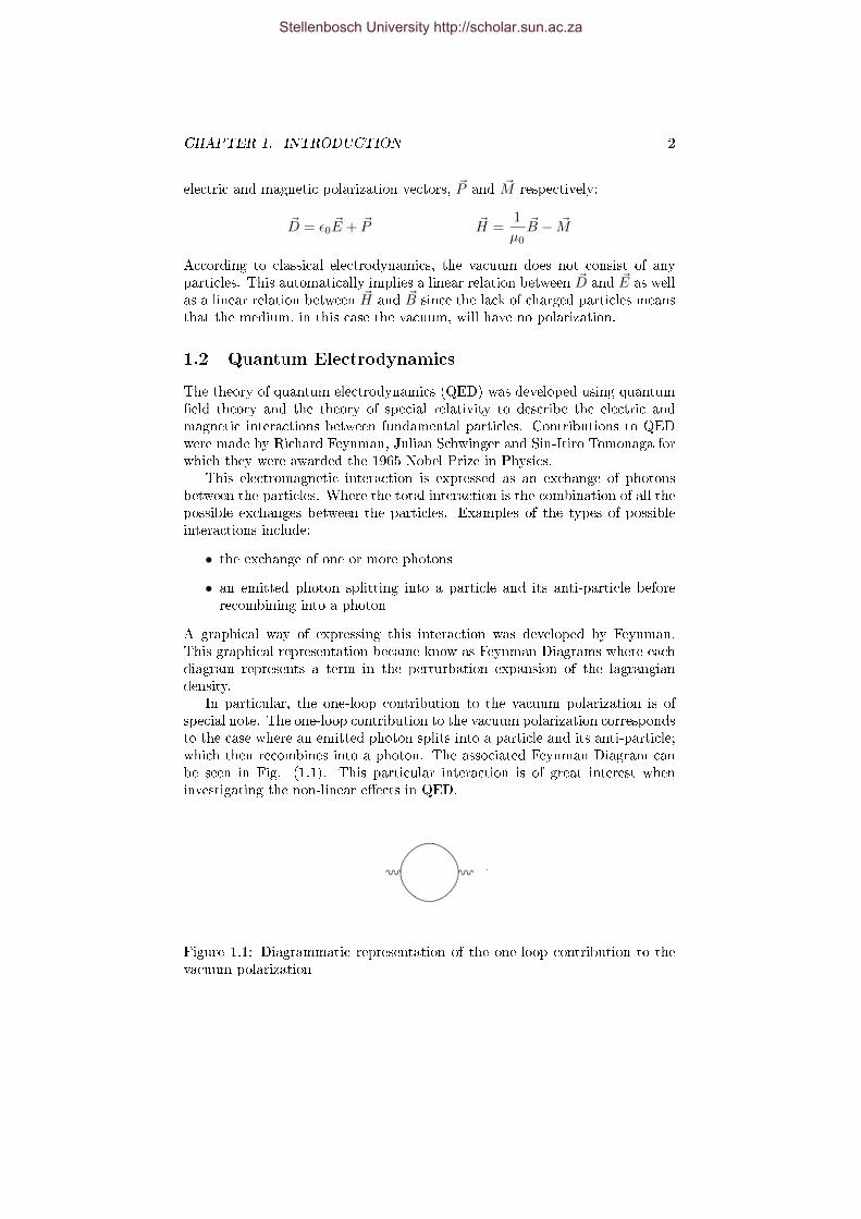
In particular, the one-loop contribution to the vacuum polarization is ofspecial note. The one-loop contribution to the vacuum polarization correspondsto the case where an emitted photon splits into a particle and its anti-particle;which then recombines into a photon. The associated Feynman Diagram canbe seen in Fig. (1.1). This particular interaction is of great interest wheninvestigating the non-linear eects in QED.

Figure 1.1: Diagrammatic representation of the one-loop contribution to thevacuum polarization



1.3 Non-Linear Quantum Electrodynamics

Non-linear processes in QED have not been investigated in great detail in thepast. The eects of these processes are much smaller than the eects producedby linear QED and thus have been dicult to detect and measure. With theadvent of modern lasers, with increasing eld intensity and peak electric eldstrength of the order 1014V/m (with 1015 − 1016V/m on the horizon), thecritical eld strength, Ec ≈ 1018V/m, may not be so far o. Many non-linearQED eects may be detectable as electric eld strengths approach this criticalvalue. Examples of these eects include :

• Spontaneous Pair Production, which refers to the spontaneous emissionof an electron-positron pair from the vacuum

• Non-linear Compton Scattering, where an electron absorbs multiple pho-tons before emitting one

Some non-linear eects such as (i) the induced magnetic eld produced byan electric charge in a constant background magnetic eld and (ii) the in-duced electric eld produced by a magnetic moment in a constant backgroundelectric eld, may be detectable with present technology. These eects are aconsequence of the Lagrangian proposed by W. Heisenberg and H. Euler intheir paper "Consequences of Dirac's Theory of the Positron" [12].

The study of non-linear processes may lead to new insight and a better un-derstanding of the physical universe. This study hopes to renew interest innon-linear QED topics and to introduce some novel eects generated by theinteraction of the electric and magnetic elds. With further research and someproposed experiments these eects may be observable with current technolo-gies.

1.4 Euler-Heisenberg Lagrangian

Euler and Heisenberg formulated their Lagrangian by investigating the ideathat electromagnetic elds can polarize the vacuum and how this polarizationaects Maxwell's equations. This polarization can be caused either by thespontaneous emission of a particle and anti-particle pair, provided that theelectromagnetic elds are strong enough, or by virtually created particle andanti-particle pairs in the vacuum. The lagrangian can derived from the one-loop eective action in the presence of a background electromagnetic eld. Thiseective action is given by [5]:

S(1) = −i ln det(i /D −m

)= − i

2ln det

(/D

2+ m2

)(1.1)



where,

/D = γµ(∂µ + ieAµ) −Dirac operator

γµ − gamma matrices usually represented by four 4x4 matrices

∂µ − derivative with respect to the space-time coordinate xµ

e − charge on an electron

m −mass of an electron

Aµ − xed classical gauge potential with eld strength tensor

Fµν = ∂µAν − ∂νAµ

For spinor QED, the one-loop eective action can be perturbatively expandedin even powers of the external photon eld Aµ. This can be represented dia-grammatically as seen in Figure 1.2. Heisenberg and Euler were able to produce

Figure 1.2: Diagrammatic representation of the one-loop eective action in thepresence of a background electromagnetic eld

an expression for the one-loop eective action in the low energy limit of theexternal photon lines (the wavy lines in Figure 1.2). Moving from the action(eqn. (1.1)) to the lagrangian requires the addition of a proper time coordinateas well as the use of the relation between the determinant (det) and the trace(tr):

det(A) = exp(tr(log(A)))

where A is a matrix, exp is the matrix exponential and log is the matrixlogarithm. After a lot of work, Euler and Heisenberg were able to producean expression for the lagrangian from the one-loop eective action (see [12]and [11]). This lagrangian became know as the Euler-Heisenberg Lagrangianand can be expressed as:

L(1)sp =

1

hc

∫ ∞0

dη

η3e−ηcεc

e2abη2

tanh(cbη)tan(caη)− 1− e2η2

3(b2 − a2)

(1.2)

where,

εc =m2c3

eh− critical eld strength

a2 − b2 = ~E2 − c2 ~B2 = −1

2FµνF

µν ≡ 2F

ab = c ~E · ~B = −1

4Fµν F

µν ≡ G



The critical eld strength, εc, is determined as the the eld strength requiredto produce an electron-positron pair out of the vacuum at a distance equal tothat of the Compton wavelength of the electron. This is achieved by writingthe energy required to produce the electron-positron pair in two dierent waysi.e. the energy required to create an electron-positron pair (2mc2) and theenergy required to move an electron and a positron, a distance equal to theirCompton wavelength (2eεc

(hmc

)). Equating these energies gives a value for the

critical eld strength:

εc =m2c3

eh

The weak eld expansion of Euler-Heisenberg Lagrangian is given by:

L(1)spinor =

2α2ε20h

45m4c5[(a2 − b2)2 + 7(ab)2

]+ · · ·

≈ 2α2ε20h

45m4c5[4F2 + 7G2

]+ · · ·

= ζ[4F2 + 7G2

]+O(ζ2) (1.3)

where α = e2

4πε0his the ne structure constant and ζ is dened as:

ζ =2α2ε20h

45m4c5

≈ 1.3× 10−52 J m

V4 (1.4)

The rst term in this expansion corresponds to the second diagram in Figure1.2. The process is know as Light-Light Scattering and is the rst non-lineareect proposed by the Euler-Heisenberg Lagrangian.

Since photons have no electric charge, produce no magnetic elds and have nomass, they cannot interact with each other. Photons are also the "informationcarriers" of the electromagnetic elds. This leads to the linear superpositionprinciple of electromagnetic elds which states that the interaction betweenany two charges is not aected by the presence of other charges [8].

The Light-Light Scattering term says that this is not entirely true. It im-plies that an electric/magnetic eld strength at a given point may be inu-enced by the background electromagnetic elds. These corrections to the elec-tric/magnetic elds are very small compared to the electric/magnetic elds andmay not be detectable. However, the induced magnetic/electric elds, whichwere not present before, may be detectable.

This investigation deals with these induced electric/magnetic elds i.e. the in-duced magnetic eld produced by an electric charge in a constant backgroundmagnetic eld and the induced electric eld produced by a magnetic dipole ina constant background electric eld.


Chapter 2

Theory

2.1 Derivation of the Induced Electric and Magnetic

Field Equations

2.1.1 Dening the Auxiliary Fields ~D and ~H

Our goal is to derive time-independent equations for the induced electric eldand the induced magnetic eld produced by an arbitrary charge (j0) and current(~j). Using eqn. (1.3), we dene the Lagrangian L as:

L = ε0F + L(1)spinor

= ε0F + ζ[4F2 + 7G2

](2.1)

We dene the electric displacement ( ~D) and the magnetization eld ( ~H) as[4, 12]:

~D =∂L∂ ~E

(2.2)

~H = − ∂L∂ ~B

(2.3)

Using the chain-rule for dierentiation ddxf(u) = df

dududx ,

∂L∂ ~E

=∂L∂F

∂F∂ ~E

+∂L∂G

∂G∂ ~E

=

(∂L∂F

)~E +

(∂L∂G

)c ~B

∂L∂ ~B

=∂L∂F

∂F∂ ~B

+∂L∂G

∂G∂ ~B

= −(∂L∂F

)c2 ~B +

(∂L∂G

)c ~E

Thus,

~D =

(∂L∂F

)~E +

(∂L∂G

)c ~B (2.4)

6


CHAPTER 2. THEORY 7

~H =

(∂L∂F

)c2 ~B −

(∂L∂G

)c ~E (2.5)

Putting in the explicit values for ∂L∂F = (ε0 + 8ζF) and ∂L

∂G = 14ζG from eqn.

(2.1), we obtain expressions for ~D and ~H.

~D = ε0 ~E +[2ζ(

4F ~E + 7cG ~B)]

≡ ε0 ~E + ~P (2.6)

In eqn. (2.6), we dene ~P ≡ 2ζ(

4F ~E + 7cG ~B)as the electric polarization

vector.

~H = − ∂L∂ ~B

= c2 (ε0 + 8ζF) ~B − 14ζGc ~E

= ε0c2 ~B + ζ

(8c2F ~B − 14cG ~E

)≡

~B

µ0− ~M (2.7)

In eqn. (2.7), we dene ~M ≡ ζ(−8c2F ~B + 14cG ~E

)as the magnetic polariza-

tion vector.

These two results are remarkably interesting. They suggest that the vacuumitself behaves like a polarizable medium. Although the vacuum contains noreal particles; quantum mechanics says that virtual particles do exist for avery short time. This shows that these virtual particles do interact but thisinteraction is very small, of the order ζ.

2.1.2 Expressions for ~E and ~B

By rewriting eqns. (2.4) and (2.5) in matrix form and inverting this matrix

equation, we can obtain an expressions for ~E and ~B in terms of the auxiliaryelds ~D and ~H. [

~D~H

]=

[∂L∂F c∂L∂G−c∂L∂G c2 ∂L∂F

] [~E~B

][~E~B

]=

1

c2(∂L∂F)2

+ c2(∂L∂G)2 [c2 ∂L∂F −c∂L∂G

c∂L∂G∂L∂F

] [~D~H

]Thus,

~E =

(∂L∂F)~D − 1

c

(∂L∂G)~H(

∂L∂F)2

+(∂L∂G)2

~B =1

c

(∂L∂G)~D + 1

c

(∂L∂F)~H(

∂L∂F)2

+(∂L∂G)2


CHAPTER 2. THEORY 8

Substituting the explicit values for ∂L∂F = (ε0 + 8ζF) and ∂L

∂G = 14ζG, we obtainobtain expressions for ~E and ~B. It is also noted, from the denition of ζ (eqn.(1.4)), that ζ is very small, of the order 10−52 in SI units. It is thus sucientfor us to only consider terms of the order ζ, since terms with higher orders inζ would be even smaller and hardly noticeable.

(∂L∂F

)2

= (ε0 + 8ζF)2

= ε20 + 16ε0ζF + 64ζ2F2

≈ ε20 + 16ε0ζF

(∂L∂G

)2

= 196ζ2G2

≈ 0

1(∂L∂F)2

+(∂L∂G)2 ≈ 1(

∂L∂F)2

≈ 1

ε20

(1 + 16 ζ

ε0F)

≈1− 16 ζ

ε0F

ε20(2.8)

Eqn. (2.8) uses the well known Taylor expansion of 11+x with the condition

x 1:

1

1 + x= 1− x+ x2 − 1

2x3 · · ·

≈ 1− x

The resulting expression for ~E and ~B are thus given by:

~E =1

ε20

[1− 16

ζ

ε0F]

(ε0 + 8ζF) ~D − 1

c(14ζG) ~H

≈ 1

ε20

(ε0 + 8ζF − 16ζF) ~D − 1

c14ζG ~H

=

(1

ε0− 8

ζ

ε20F)~D − 1

cε20(14ζG) ~H (2.9)

~B =1

cε20

[1− 16

ζ

ε0F]

(14ζG) ~D +1

c(ε0 + 8ζF) ~H

≈ 1

cε20

(14ζG) ~D +

ε0c~H − 16

ζ

cF ~H + 8

ζ

cF ~H

=

1

cε20(14ζG) ~D +

1

c2

(1

ε0− 8

ζ

ε20F)~H (2.10)


CHAPTER 2. THEORY 9

2.1.3 General Solutions using Maxwell's Equations

Maxwell's equations for quasi-static background electric and magnetic eldsare given by:

~∇ · ~D = j0 ~∇× ~E = 0 (2.11)

~∇ · ~B = 0 ~∇× ~H = ~j (2.12)

where j0 is the charge and ~j is the current. It must also be noted that theseare the time-independent equations. The general solutions for ~D and ~H canbe written as :

~D = ~DM + ~∇× ~K (2.13)

~H = ~HM + ~∇φ (2.14)

In the above equations (2.13 and 2.14), ~DM and ~HM refer to the generalsolutions of the Maxwell theory, namely the background electric and magneticelds as well as those elds produced by the charge, j0, and the current, ~j. Allother terms are contained in ~∇× ~K and ~∇φ. The form of these terms ensurethat ~∇ · ~D = j0, ~∇ × ~H = ~j, ~∇ × ~D = 0 and ~∇ · ~H = 0. Considering thequasi-static situation, we introduce a constant electric background eld ( ~E0)

as well as a constant magnetic background eld ( ~B0) to produce expressions

for ~DM and ~HM :

~DM = ε0 ~E0 −1

4π~∇x∫

j0(~y)

|~x− ~y|d3y

~HM =~B0

µ0+

1

4π~∇x ×

∫ ~j(~y)

|~x− ~y|d3y

Consider ~∇ · ~B = 0 (eqn. (2.12)),

~∇ · ~B = 0 =14ζ

ε20c~∇ ·(G ~D)

+1

c2

1

ε0~∇ · ~H − 8ζ

ε20~∇ ·(F ~H

)Substituting ~∇ · ~H = ∇2φ gives:

0 = ~∇ ·

14ζ

ε20cG ~D − 8ζ

ε20c2F ~H

+

1

ε0c2∇2φ

~∇ ·

14ζ

ε20cG ~D − 8ζ

ε20c2F ~H

= −~∇ ·

1

ε0c2~∇φ

(2.15)

Following Helmholtz's Theorem [9], the solution for 1ε0c2

~∇φ in eqn. (2.15) canbe expressed as:

1

ε0c2~∇φ(~x) =

1

4π~∇x∫

d3y

~∇y ·

14ζε20cG ~D − 8ζ

ε20c2F ~H

|~x− ~y|

(2.16)

A similar treatment can be used on ~∇× ~E = 0 (eqn. (2.11)) such that:

~∇×(

1

ε0~∇× ~K

)= ~∇×

8ζ

ε20F ~D +

14ζ

ε20cG ~H

(2.17)


CHAPTER 2. THEORY 10

~∇× ~K(~x) =ε04π

~∇x ×∫

d3y

~∇y ×

8ζε20F ~D + 14ζ

ε20cG ~H

|~x− ~y|(2.18)

It is also noted from eqns. (2.16) and (2.18) that ~∇φ(~x) and ~∇ × ~K(~x) areboth at least of the order ζ.

2.1.4 Obtaining the Induced Fields ~E and ~BWe now dene the induced electric eld (~E(~x)) as the dierence between theelectric eld (as dened in eqn. (2.9)) and the Maxwell electric eld.

~E(~x) ≡ ~E(~x)− 1

ε0~DM (~x) (2.19)

Similarly, the induced magnetic eld ( ~B(~x)) can be dened as the dierencebetween the magnetic eld (as dened in eqn. (2.10)) and the Maxwell magneticeld.

~B(~x) ≡ ~B(~x)− µ0~HM (~x) (2.20)

Using eqns. (2.9) and (2.13), we can express ~E as:

~E =1

ε0~DM +

1

ε0~∇× ~K +

−8ζ

ε20F ~D − 14ζ

ε20cG ~H

(2.21)

Thus,

~E(~x) =1

ε0~∇× ~K − ζ

8

ε20F ~D +

14

ε20cG ~H

(2.22)

~∇× ~E(~x) =1

ε0~∇× ~∇× ~K − ζ ~∇×

8

ε20F ~D +

14

ε20cG ~H

= 0 , using eqn (2.17) (2.23)

This result is not surprising since ~∇× ~E = 0 and ~∇× ~DM = 0.

~∇ · ~E(~x) = −ζ ~∇ ·

8

ε20F ~D +

14

ε20cG ~H

(2.24)

Using Helmholtz's theorem [9] and the fact that ~∇ × ~E = 0, it can be shownthat

~E = −~∇ψ (2.25)

where, ψ is a scalar function. Helmholtz's theorem also gives a general solutionfor ψ:

ψ =1

4π

∫d3y

~∇ · ~E|~x− ~y|

(2.26)

Bringing eqns. (2.24), (2.25) and (2.26) together gives us an expression for ~E :

~E(~x) =ζ

4πε20~∇x∫

d3y

|~x− ~y|~∇y ·

8F ~D +

14

cG ~H

(2.27)



Consider ζF ~D and ζG ~H; only keeping terms of the order ζ (O(ζ))

ζF ~D = ζ(E2 − c2B2

)~D

= ζ

((~EM + ~E

)2

− c2(~BM + ~B

)2)~D ,eqns. (2.19) and (2.20)

= ζ(E2M + 2~E · ~EM + E2 − c2B2

M − 2c2 ~BM · ~B − c2B2)~D

= ζ(E2M − c2B2

M

)~D +O(ζ2) ,~E and ~B are O(ζ)

≈ ζFM ~D

= ζFM(~DM + ~∇× ~K

),eqn. (2.13)

= ζFM ~DM +O(ζ2) , ~∇× ~K is O(ζ) (eqn. (2.18))

≈ ζFM ~DM (2.28)

ζG ~H = cζ(~E · ~B

)~H

= cζ(~EM + ~E

)·(~BM + ~B

)~H ,eqns. (2.19) and (2.20)

= cζ[~EM · ~BM + ~EM · ~B + ~E · ~BM + ~E · ~B

]~H

= cζ ~EM · ~BM +O(ζ2) ,~E and ~B are O(ζ)

≈ ζGM ~H

= ζGM(~HM + ~∇φ

),eqn. (2.13)

= ζGM ~HM +O(ζ2) ,~∇φ is O(ζ) (eqn. (2.16))

≈ ζGM ~HM (2.29)

In eqns. (2.28) and (2.29), FM and GM refer to the Lorentz invariants F andG when the Maxwell elds are the only elds present. The nal form of theinduced electric eld is thus:

~E(~x) =ζ

4πε20~∇x∫

d3y

|~x− ~y|~∇y ·

8FM ~DM +

14

cGM ~HM

(2.30)

A similar procedure is used to obtain an expression for the induced magneticeld. Using eqns. (2.10) and (2.14), ~B can be expressed as:

~B = µ0~HM + µ0

~∇φ+

− 8ζ

c2ε20F ~H +

14ζ

ε0cG ~D

(2.31)

Thus,

~B(~x) = µ0~∇φ+

− 8ζ

ε20c2F ~H +

14ζ

ε20cG ~D

(2.32)

Using a similar procedure as that used to obtain ~∇ × ~E = 0, it can be showthat ~∇ · ~B = 0 using eqn. (2.15). Calculating ~∇ · ~B gives :

~∇× ~B(~x) =ζ

ε20c~∇×

−8

cF ~H + 14G ~D

(2.33)



Using Helmholtz's Theorem and the fact that ~∇ · ~B = 0, B can be expressedas:

~B = ~∇× ~A (2.34)

where ~A is a vector function and is given by :

~A =1

4π

∫d3y

~∇× ~B|~x− ~y|

(2.35)

Bringing eqns. (2.33), (2.34) and (2.35) together produces the expression :

~B(~x) =ζ

4πε20c~∇x ×

∫d3y

|~x− ~y|~∇y ×

−8

cF ~H + 14G ~D

(2.36)

Similarly to eqns. (2.28) and (2.29), F ~H and G ~D can be replaced by FM ~HM

and GM ~DM respectively without aecting ~B to leading order in ζ. The nalform of the induced magnetic eld is thus:

~B(~x) =ζ

4πε20c~∇x ×

∫d3y

|~x− ~y|~∇y ×

−8

cFM ~HM + 14GM ~DM

(2.37)

2.2 Summary and Discussion

In deriving the equations for the induced electric and magnetic eld, we ndthat the electric displacement (eqn. (2.6)) and the magnetization (eqn. (2.7))can be expressed as follows:

~D = ε0 ~E + ~P

~H =~B

µ0− ~M

where,

~P = 2ζ(

4F ~E + 7cG ~B)

~M = 2ζ(

4c2F ~B − 7cG ~E)

The derivation of ~D and ~H did not assume the presence of a medium but here itcan be seen that there are terms that look like the electric polarization vector(~P ) and magnetic polarization vector ( ~M). This strange behaviour can beunderstood as the vacuum behaving as a polarized medium. This polarizationis very small since ~P and ~M are both proportional to ζ. As ζ → 0, ~P and ~Mwill vanish. The main result is the derivation of the equations for the inducedelectric eld (eqn. (2.30)) and the induced magnetic eld (eqn. (2.37)):

~E(~x) =ζ

4πε20~∇x∫

d3y

|~x− ~y|~∇y ·

8FM ~DM +

14

cGM ~HM

~B(~x) =

ζ

4πε20c~∇x ×

∫d3y

|~x− ~y|~∇y ×

−8

cFM ~HM + 14GM ~DM

It must be noted that the quantum eects are contained within the factor ζ.On the other hand, the factors FM , GM , ~DM and ~HM are all obtained fromclassical sources and external elds. This is very handy, since ~E and ~B can nowbe handled as classical time-independent objects.


Chapter 3

Investigating the Induced Fields

3.1 Charged Shell in a Quasi-static Magnetic Field

3.1.1 The Situation

Consider a charged spherical shell of radius R, which carries a uniform surfacecharge, in the presence of an external magnetic eld, ~B0 (see Figure 3.1). Theelectric eld produced by the spherical shell is known and is given by:

~EM (~x) =1

ε0~DM =

Q

4πε0

Θ(r −R)

r2er (3.1)

where,

~x = (r, θ, φ) - position vector in spherical coordinates

r - radius with the unit vector er

θ - polar angle with the unit vector eθ

φ - azimuthal angle with the unit vector eφ

Q - total charge on the shell

Figure 3.1: A charged shell in an external magnetic eld

13


CHAPTER 3. INVESTIGATING THE INDUCED FIELDS 14

The external magnetic eld is orientated along the z-axis and has a eldstrength B0. ~B0 is given by:

~B0 = B0ez = B0 (cos(θ)er − sin(θ)eθ) (3.2)

Eqns. (3.1) and (3.2) give rise to the following expressions:

FM =1

2

[E2M + c2B2

0

]=

1

2

[(Q

4πε0

)21

r4Θ(r −R)− c2B2

0

](3.3)

GM = c ~EM · ~B0

=cQB0

4πε0

cos(θ)

r2Θ(r −R) (3.4)

~DM =Q

4π

1

r2Θ(r −R)er (3.5)

~HM =B0

µ0(cos(θ)er − sin(θ)eθ) (3.6)

Dene ~V1 and ~V2 as:

~V1(~x) ≡ 4FM (~x) ~DM (~x) +7

cGM (~x) ~HM (~x) (3.7)

~V2(~x) ≡ −4

cFM (~x) ~HM (~x) + 7GM (~x) ~DM (~x) (3.8)

such that eqns. (2.30) and (2.37) become:

~E(~x) =2ζ

4πε20~∇x∫

d3y

|~x− ~y|~∇y · ~V1(~y) (3.9)

~B(~x) =2ζ

4πε20c~∇x ×

∫d3y

|~x− ~y|~∇y × ~V2(~y) (3.10)

3.1.2 Calculating ~E(~x)

Substituting eqns. (3.3), (3.4), (3.5) and (3.6) into eqn. (3.7):

~V1(~x) =2Q

4π

[(Q

4πε20

)21

r6Θ(r −R)er − c2B2

0

1

r2Θ(r −R)er

]

+ 7QB2

0

4πε0µ0

[cos2(θ)

r2Θ(r −R)er −

cos(θ)sin(θ)

r2Θ(r −R)eθ

]



Thus,

~∇ · ~V1(~x) =

2Q

4π

[(Q

4πε0

)2

~∇ ·(

1

r6Θ(r −R)er

)− c2B2

0~∇ ·(

1

r2Θ(r −R)er

)]

+ 7QB2

0

4πε0µ0

[~∇ ·(cos2(θ)

r2Θ(r −R)er

)− ~∇ ·

(cos(θ)sin(θ)

r2Θ(r −R)eθ

)]

=

2Q

4π

[(Q

4πε

)2δ(r −R)

r6− 4

Θ(r −R)

r7

− c2B2

0

δ(r −R)

r2

]

+ 7QB2

0

4πε0µ0

[cos2(θ)

r2δ(r −R)− 3cos2(θ)− 1

r3Θ(r −R)

](3.11)

We now introduce the following notation:

• ~y = (r′, θ′, φ′) as a position vector

• Ωx = (θ, φ)

• Ωy = (θ′, φ′)

• Ylm(Ωx) = Ylm is the spherical harmonic of degree l and order m

• Ylm(Ωy) = Y ′lm

Using a table of spherical harmonics [10], we can introduce spherical harmonicfunctions into eqn. (3.11):

1 = Y00

√4π

cos2(θ) =1

3

√16π

5Y20 +

1

3

√4πY00

3cos2(θ)− 1 =

√16π

5Y20

~∇ · ~V1(~x) =

2Q

4π

[(Q

4πε

)2δ(r −R)

r6− 4

Θ(r −R)

r7

− c2B2

0

δ(r −R)

r2

]Y00

√4π

+ 7QB2

0

4πε0µ0

[1

3

δ(r −R)

r2

√16π

5Y20 +

√4πY00

− Θ(r −R)

r3

√16π

5Y20

](3.12)

Using the following identity, we can rewrite eqn. (3.9):

1

|~x− ~y|=∑l,m

4π

2l + 1

rl<rl+1>

Ylm(Ωx)Y ∗lm(Ωy) (3.13)

Note that if r > r′ then r> = r, conversely if r < r′ then r> = r′.~E(~x) is thus,

~E(~x) =2ζ

4πε20~∇x∑l,m

4π

2l + 1

∫ ∞0

dr′ r′2rl<rl+1>

∫dΩyYlmY

′∗lm~∇ · ~V1(~y) (3.14)



The orthogonality relation of spherical harmonic functions is given by:∫dΩ Ylm(Ω)Yl′m′(Ω) = δll′δmm′ (3.15)

Substituting eqn. (3.12) into eqn. (3.14) and applying eqn. (3.15) gives:

~E(~x) =2ζ

4πε20~∇x∑l,m

4π

2l + 1Ylm

∫ ∞0

dr′ r′2rl<rl+1>

2Q

4π

[(Q

4πε

)2δ(r′ −R)

r′6− 4

Θ(r′ −R)

r′7

−c2B20

δ(r′ −R)

r′2

]δl0δm0

√4π + 7

QB20

4πε0µ0

[1

3

δ(r′ −R)

r′2

√16π

5δl2δm0 +

√4πδl0δm0

−Θ(r′ −R)

r′3

√16π

5δl2δm0

]

=2ζ

ε20~∇x

2Q

4π

[(Q

4πε

)2∫ ∞0

dr′δ(r′ −R)

rr′4− 4

∫ ∞0

dr′Θ(r′ −R)

r>r′5

−c2B20

∫ ∞0

dr′δ(r′ −R)

r

]Y00

√4π + 7

QB20

4πε0µ0

[1

3

1

5

√16π

5

∫ ∞0

dr′r′2δ(r′ −R)

r3Y20

+√

4π

∫ ∞0

dr′δ(r′ −R)

rY00

−∫ ∞

0

dr′r<Θ(r′ −R)

r2>r′

√16π

5Y20

]

Note that ~E(~x) will always be evaluated at a point far away from the surfaceof the shell. Therefore terms with δ(r′−R) as factors will always have r> = r.

After integrating and simplifying ~E(~x) is given by:

~E(~x) = −~∇x

[− 4ζ

5ε40

(Q

4π

)31

r5− QB2

0ζ

4πε30µ0

7

3

(3cos2(θ)− 1

) R2

r3−(7cos2(θ)− 3

) 1

r

](3.16)

Dening the scalar functions

V1 = − 4ζ

5ε40

(Q

4π

)31

r5

V2 = − 7QB20ζ

12πε30µ0

(3cos2(θ)− 1

) R2

r3

V3 =QB2

0ζ

4πε30µ0

(7cos2(θ)− 3

) 1

r

Such that ~E(~x) = −~∇x [V1 + V2 + V3].The scalar potential V of a charged spherical shell of radius R and charge Q isgiven by:

V =1

4πε0

Q

r



Using ζ ≈ 10−52, ε0 ≈ 10−11 and µ0 ≈ 10−6 (in SI units); we can now comparethe relative strengths of the scalar functions V1,V2 and V3:

V1

V= − 4ζ

5ε20(4π)2

Q2

r4≈ −10−20Q

2

r4

V2

V= −7

3(cos2(θ)− 1)

ζ

ε20µ0

B20R

2

r2≈ −10−24B

20R

2

r2

V3

V= (7cos2(θ)− 3)

ζ

ε20µ0B2

0 ≈ 10−24B20

From these relations, it is clear that the V1, V2 and V3 are very much smallerthan the electric potential of the charged spherical shell. This means that ~E(~x)

will be overpowered by the more powerful electric eld ~EM (~x).

3.1.3 Calculating ~B(~x)

An explicit expression for ~V2 can be obtained by using eqn. (3.3), (3.4), (3.5)and (3.6)

~V2 = −4

cFM ~HM + 7GM ~DM

=B0

µ0

[5

(Q

4πε0

)2cos(θ)

r4Θ(r −R)er + 2

(Q

4πε0

)2sin(θ)

r4Θ(r −R)eθ − 2c2B2

0 (cos(θ)er − sin(θ)eθ)

]

The curl of ~V2 can now be calculated:

~∇× ~V2 =B0

µ0c

(Q

4πε0

)2 [2δ(r −R)

r4− Θ(r −R)

r5

]sin(θ)eφ

Using a table of spherical harmonics, it is possible to show that:

sin(θ)eφ = sin(θ) (−sin(φ)ex + cos(φ)ey)

= −sin(θ)sin(φ)ex + sin(θ)cos(φ)ey

=

√8π

3

(Y11 + Y1−1

2iex −

Y11 − Y1−1

2ey

)Thus ~∇× ~V2 becomes

~∇× ~V2 =B0

µ0c

(Q

4πε0

)2 [2δ(r −R)

r4− Θ(r −R)

r5

]√8π

3

[Y11 + Y1−1

2iex −

Y11 − Y1−1

2ey

]Using the same identity (eqn. (3.13)) as was used to calculate ~E (eqn. (3.14)),~B can expressed as:

~B(~x) =2ζ

4πε20c~∇x∫

d3y∑l,m

4π

2l + 1

rl<rl+1>

YlmY′∗lm~∇y × ~V2



Thus,

~B(~x) =2ζB0

ε0

(Q

4πε0

)2

~∇x ×∑l,m

1

2l + 1

∫ ∞0

dr′ r′2rl<rl+1>

Ylm

[2δ(r′ −R)

r′4

−Θ(r′ −R)

r′5

]√8π

3

[δl1δm1 + δl1δm−1

2iex −

δl1δm1 − δl1δm−1

2ey

]=

2ζB0

3ε0

(Q

4πε0

)2

~∇x ×∫ ∞

0

dr′r<r2>

[2δ(r′ −R)

r′2

−Θ(r′ −R)

r′3

]√8π

3

(Y11 + Y1−1

2iex −

Y11 − Y1−1

2ey

)After completing the integration and simplifying, the nal form of ~B can beexpressed as:

~B(~x) = ~∇x ×

[2ζB0

3ε0

(Q

4πε0

)21

r2R+

3

4r3

sin(θ)eφ

](3.17)

From eqn. (3.17), one can associate the vector potential ~A with:

~A =2ζB0

3ε0

(Q

4πε0

)21

r2R+

3

4r3

ez × er (3.18)

3.1.4 Summary and Discussion

It must be noted that there is a restriction to r. This restriction arises fromthe fact that | ~EM | < 1.3× 1018V/m. In other words:

| ~EM | =Q

4πε0

1

r2< 1.3× 1018

r2 > 1.3× 10−18 Q

4πε0

Thus,

r > 8.3√Q× 10−5

where r is measured in meters and Q in coulombs. However, this means that ifwe use the shell as a model for the proton then we cannot get too close to theproton since its size is of the order 10−15m which is less than the restriction8.3√

1.9× 10−19 × 10−5m ≈ 3.6× 10−14m.

The induced electric eld produced by the interaction of the charged spher-ical shell and the quasi-static magnetic eld is given in eqn. (3.16). Thisinduced electric eld is much smaller than the eld produced by the chargedspherical shell and will therefore be much more dicult to detect.

The induced magnetic eld produced by the interaction of the charged sphericalshell and quasi-static magnetic eld is given by eqn. (3.17):

~B(~x) = ~∇x ×

[2ζB0

3ε0

(Q

4πε0

)21

r2R+

3

4r3

sin(θ)eφ

]



The vector eld that can be associated with the induced magnetic eld is givenby eqn. (3.18):

~A =2ζB0

3ε0

(Q

4πε0

)21

r2R+

3

4r3

ez × er

If r R, which can be expected in an experimental setup, then the 1r2R term

dominates 34r3 . Thus,

~A =2ζ

3ε0

(Q

4πε0

)21

r2R~B0 × er

This vector potential is the same as that produced by the magnetic dipolemoment:

~m =c2ζ

6πε20

Q2

R~B0 (3.19)

where ~A = µ0

4π~m×err2

Although this induced magnetic dipole is small, of the order ζ, it did not existbefore and should therefore be detectable. When considering an experimentalsetup; the total charge Q, radius of the shell R and the external quasi-staticmagnetic eld ~B0 should be chosen in such a way to maximize the inducedmagnetic moment ~m.

3.2 Spherical Magnetic Dipole in a Quasi-static Electric

Field

3.2.1 The Situation

Figure 3.2: A spherical magnetic moment in an external electric eld



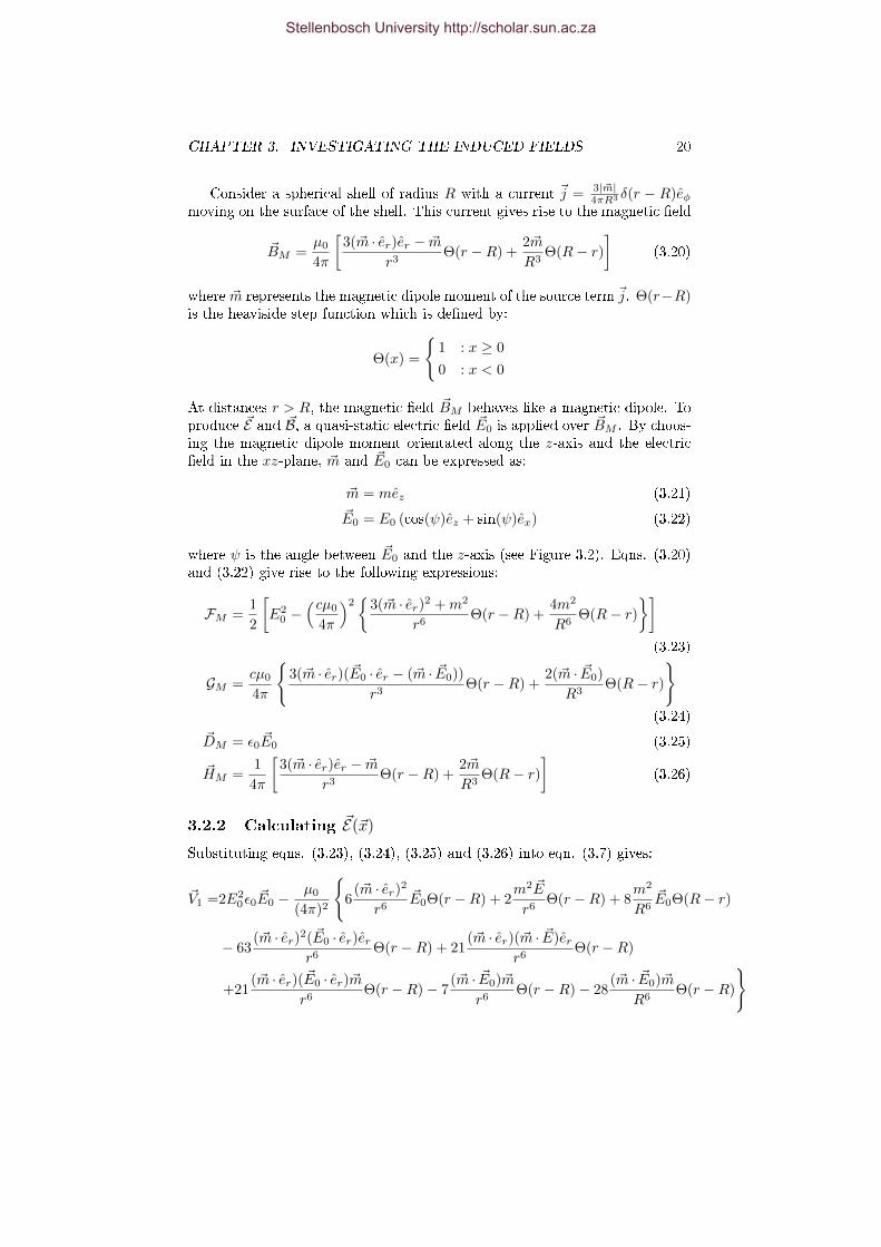
Consider a spherical shell of radius R with a current ~j = 3|~m|4πR3 δ(r − R)eφ

moving on the surface of the shell. This current gives rise to the magnetic eld

~BM =µ0

4π

[3(~m · er)er − ~m

r3Θ(r −R) +

2~m

R3Θ(R− r)

](3.20)

where ~m represents the magnetic dipole moment of the source term ~j. Θ(r−R)is the heaviside step function which is dened by:

Θ(x) =

1 : x ≥ 0

0 : x < 0

At distances r > R, the magnetic eld ~BM behaves like a magnetic dipole. Toproduce ~E and ~B, a quasi-static electric eld ~E0 is applied over ~BM . By choos-ing the magnetic dipole moment orientated along the z-axis and the electriceld in the xz-plane, ~m and ~E0 can be expressed as:

~m = mez (3.21)

~E0 = E0 (cos(ψ)ez + sin(ψ)ex) (3.22)

where ψ is the angle between ~E0 and the z-axis (see Figure 3.2). Eqns. (3.20)and (3.22) give rise to the following expressions:

FM =1

2

[E2

0 −(cµ0

4π

)2

3(~m · er)2 +m2

r6Θ(r −R) +

4m2

R6Θ(R− r)

](3.23)

GM =cµ0

4π

3(~m · er)( ~E0 · er − (~m · ~E0))

r3Θ(r −R) +

2(~m · ~E0)

R3Θ(R− r)

(3.24)

~DM = ε0 ~E0 (3.25)

~HM =1

4π

[3(~m · er)er − ~m

r3Θ(r −R) +

2~m

R3Θ(R− r)

](3.26)

3.2.2 Calculating ~E(~x)

Substituting eqns. (3.23), (3.24), (3.25) and (3.26) into eqn. (3.7) gives:

~V1 =2E20ε0 ~E0 −

µ0

(4π)2

6

(~m · er)2

r6~E0Θ(r −R) + 2

m2 ~E

r6Θ(r −R) + 8

m2

R6~E0Θ(R− r)

− 63(~m · er)2( ~E0 · er)er

r6Θ(r −R) + 21

(~m · er)(~m · ~E)err6

Θ(r −R)

+21(~m · er)( ~E0 · er)~m

r6Θ(r −R)− 7

(~m · ~E0)~m

r6Θ(r −R)− 28

(~m · ~E0)~m

R6Θ(r −R)



Performing the divergence of ~V1 produces:

~∇ · ~V1 =− µ0

(4π)2

6~∇ ·

[(~m · er)2

r6~E0Θ(r −R)

]+ 2~∇ ·

[m2 ~E

r6Θ(r −R)

]+ 8~∇ ·

[m2

R6~E0Θ(R− r)

]

− 63~∇ ·

[(~m · er)2( ~E0 · er)er

r6Θ(r −R)

]+ 21~∇ ·

[(~m · er)(~m · ~E)er

r6Θ(r −R)

]

+ 21~∇ ·

[(~m · er)( ~E0 · er)~m

r6Θ(r −R)

]− 7~∇ ·

[(~m · ~E0)~m

r6Θ(r −R)

]

−28~∇ ·

[(~m · ~E0)~m

R6Θ(r −R)

]

=µ0

(4π)2

9

(~m · er)(~m · ~E0)

r7Θ(r −R)− 36

(~m · er)2( ~E0 · er)r7

Θ(r −R)− 9m2( ~E0 · er)

r7Θ(r −R)

−42(~m · er)(~m · ~E0)

r6δ(r −R) + 36

(~m · er)2( ~E0 · er)r6

δ(r −R) + 6m2( ~E0 · er)

r6δ(r −R)

(3.27)

From the denition of ~m (eqn. 3.21) and ~E0 (eqn. 3.22), the following identitiescan be obtained:

~m · er = mcos(θ) (3.28)

~m · ~E0 = mE0cos(ψ) (3.29)

~E0 · er = E0 [sin(ψ)sin(θ)cos(φ) + cos(ψ)cos(θ)] (3.30)

Using the table of spherical harmonics [10], it is possible to show that:

cos2(θ)sin(θ)cos(φ) =1

5

1

2

[√16π

21−Y31 + Y3−1+

√8π

3−Y11 + Y1−1

](3.31)

cos3(θ) =1

5

[√16π

7Y30 + 3

√4π

3Y10

](3.32)

sin(θ)cos(φ) =1

2

√8π

3−Y11 + Y1−1 (3.33)

cos(θ) =

√4π

3Y10 (3.34)



Using the identities (3.28)-(3.30) on eqn. (3.27) then converting to sphericalharmonics gives:

~∇ · ~V1 =µ0m

2E0

(4π)2

9cos(ψ)cos(θ)

r7Θ(r −R)− 36

cos2(θ)(sin(ψ)sin(θ)cos(φ) + cos(ψ)cos(θ))

r7Θ(r −R)

− 9sin(ψ)sin(θ)cos(φ) + cos(ψ)cos(θ)

r7Θ(r −R)− 42

cos(ψ)cos(θ)

r6δ(r −R)

+ 36cos2(θ)(sin(ψ)sin(θ)cos(φ) + cos(ψ)cos(θ))

r6δ(r −R)

+6sin(ψ)sin(θ)cos(φ) + cos(ψ)cos(θ)

r6δ(r −R)

=µ0m

2E0

(4π)2

9

r7

[−sin(ψ)

1

2

√8π

3−Y11 + Y1−1 − 4cos(ψ)

1

5

[√16π

7Y30 + 3

√4π

3Y10

]

−4sin(ψ)1

5

1

2

[√64π

21−Y31 + Y3−1+

√8π

3−Y11 + Y1−1

]]Θ(r −R)

+6

R6

[cos(ψ)

√4π

3Y10 + sin(ψ)

1

2

√8π

3−Y11 + Y1−1

+ 6cos(ψ)1

5

[√16π

7Y30 + 3

√4π

3Y10

]+

6

5sin(ψ)

1

2

[√64π

21−Y31 + Y3−1

+

√8π

3−Y11 + Y1−1

]− 7cos(ψ)

√4π

3Y10

]δ(r −R)

Computing eqn. (3.14) and then applying the orthogonality relation of spher-ical harmonics (eqn. (3.15)) gives:

~E(~x) =2ζµ0m

2E0

(4π)3ε20~∇x∑l,m

4π

2l + 1Ylm

∫ ∞0

dr′ r′2rl<rl+1>

9

r7

[−sin(ψ)

1

2

√8π

3−δl1δm1 + δl1δm−1

− 4cos(ψ)1

5

[√16π

7δl3δm0 + 3

√4π

3δl1δm0

]

−4sin(ψ)1

5

1

2

[√64π

21−δl3δm1 + δl3δm−1+

√8π


]]Θ(r −R)

+6

R6

[cos(ψ)

√4π

3δl1δm0 + sin(ψ)

1

2

√8π


+ 6cos(ψ)1

5

[√16π

7δl3δm0 + 3

√4π

3δl1δm0

]+

6

5sin(ψ)

1

2

[√64π


+

√8π


]− 7cos(ψ)

√4π

3δl1δm0

]δ(r −R)



Computing the integration and then simplifying produces the nal form of theinduced electric eld ~E(~x) of the spherical magnetic dipole:

~E(~x) =− ~∇x

1

4πε0

ζµ0m2E0

πε0

[18

5cos(ψ)cos(θ)

1

R3r2− 9

4cos(ψ)cos3(θ)

1

r5+

3

10cos(ψ)cos(θ)

1

r5

(3.35)

−13

10sin(ψ)sin(θ)cos(φ)

1

R3r2− 9

4sin(ψ)sin(θ)cos2(θ)cos(φ)

1

r5

](3.36)

From the expression for the induced electric eld (eqn. (3.36)), we can see that~E(~x) has a complicated angular dependence. By only considering the terms ofthe order 1

r2 , we nd that

~E(~x) =− ~∇

1

4πε0

ζµ0m2E0

πε0

[18

5cos(ψ)cos(θ)− 13

5sin(ψ)sin(θ)cos(φ)

]1

R3r2

=− ~∇

1

4πε0

ζµ0m2E0

10πε0R3

1

r2[36(cos(ψ)cos(θ) + sin(ψ)sin(θ)sin(φ))

−49sin(ψ)sin(θ)cos(φ)]

=− ~∇

1

4πε0

ζµ0m2E0

10πε0R3

1

r2

[36~E0 · erE0

− 49( ~E0 · ex)(ex · er)

E0

](3.37)

From eqn. (3.37), we can associate the the electric dipole moment ~pψ with:

~pψ =ζµ0m

2E0

10πε0R3

[36~E0

E0− 49

( ~E0 · ex)exE0

](3.38)

such that ~E(~x) = −~∇[

14πε0

1r2 ~pψ · er

]. If we now set ~E0||~m then ~pψ reduces to

~p =36ζµ0m

2E0

10πε0R3ez (3.39)

3.2.3 Calculating ~B(~x)

Considering that there is already a classical magnetic eld ~BM which exists, itis expected that the induced magnetic eld ~B, which is of the order ζ (see eqn.(2.19)), may be too small to be observable. Using the vector identity

~∇×[f ~A]

= f[∇× ~A

]+ [∇f ]× ~A



together with eqns. (3.23), (3.24), (3.25) and (3.26); an expression for ~V2 (eqn.(3.8)) can be obtained:

~∇× ~V2 =~∇×−4

cFM ~HM + 7GM ~DM

=− 4

cGM

[~∇× ~HM

]− 4

c

[~∇GM

]× ~HM + 7

[~∇FM

]× ~DM

=1

4πc

6E2

0

er × ~m

r3δ(r −R) +

(µ0c

4π

)2[12

(~m · er)2(er × ~m)

r10Θ(r −R)

+ 12m2(er × ~m)

r10Θ(r −R)− 6

(~m · er)2(er × ~m)

r9δ(r −R)

−18m2(er × ~m)

r9δ(r −R)

]+ 21

(~m× ~E0)( ~E0 · er)r4

Θ(r −R)

− 105(~m · er)( ~E0 · er)(er × ~E0)

r4Θ(r −R) + 21

(~m · ~E0)(er × ~E0)

r4Θ(r −R)

+21(~m · er)( ~E0 · er)(er × ~E0)

r3δ(r −R)− 21

(~m · ~E0)(er × ~E0)

r3δ(r −R)

(3.40)

Using the denitions of ~m and ~E0, the following identities can be derived:

~m× ~E0 = mE0sin(ψ)ey

er × ~E0 = E0 [cos(ψ)sin(θ)sin(φ)ex + (sin(ψ)cos(θ)− cos(ψ)sin(θ)cos(φ)) ey − sin(ψ)sin(θ)sin(φ)ez]

er × ~m = msin(θ) [sin(φ)ex − cos(φ)ey]

All that is left is to perform the integration (eqn. (3.9)). To get a feel for the

magnitude of ~B, we consider the following terms:∫d3y

1

|~x− ~y|e′r × ~m

r′3δ(r′ −R) =

4π

3

1

r2er × ~m (3.41)

∫d3y

1

|~x− ~y|(~m · e′r)2(e′r × ~m)

r′9δ(r′ −R) =m2

4π

7

1

R4r4

1

5(5cos2(θ)− 1)er × ~m

+4π

3

1

R6r2

1

5er × ~m

(3.42)

∫d3y

1

|~x− ~y|m2(e′r × ~m)

r′9δ(r′ −R) =m2 4π

3

1

R6r2er × ~m (3.43)

∫d3y

1

|~x− ~y|(~m · e′r)2(e′r × ~m)

r′10Θ(r′ −R) =m2

[4π

7

7

44

1

r8+

1

4

1

R4r4

1

5(5cos2(θ)− 1)er × ~m

+4π

3

1

6

1

R6r2− 1

18

1

r8

1

5er × ~m

](3.44)



∫d3y

1

|~x− ~y|m2(e′r × ~m)

r′10θ(r′ −R) =m2 4π

3

1

6

1

R6r2− 1

18

1

r8

er × ~m (3.45)

∫d3y

1

|~x− ~y|( ~E0 · e′r)(~m× ~E)

r′4Θ(r′ −R) =mE2

0

4π

3

1

r2lnr

R+

1

3

1

r2

( ~E0 · er)(~m× ~E0)

(3.46)

∫d3y

1

|~x− ~y|(~m · e′r)( ~E0 · e′r)(e′r × ~E0)

r′3δ(r′ −R) = mE2

0

4π

7

R2

r4[1

2sin(ψ)cos(ψ)sin2(θ)cos(θ)sin(2φ)ex

+1

5cos2(ψ)sin(θ)(5cos2(θ)− 1)sin(φ)ex −

1

5cos(2ψ)sin(θ)(5cos3(θ)− 1)cos(φ)ey

+3

10cos(ψ)sin(ψ)(5cos2(θ)− 3cos(θ))ey −

1

2cos(ψ)sin(ψ)sin2(θ)cos(θ)cos(2φ)ey

−1

2sin2(ψ)sin2(θ)cos(θ)sin(2φ)ez −

1

5cos(ψ)sin(ψ)sin(θ)(5cos2(θ)− 1)sin(φ)ez

]+

4π

3

1

r2

[1

5cos2(ψ)sin(θ)sin(φ)ex −

1

5cos(2ψ)sin(θ)cos(φ)ey +

4

10cos(ψ)sin(ψ)cos(θ)ey

−1

5cos(ψ)sin(ψ)sin(θ)sin(φ)ez

](3.47)

∫d3y

1

|~x− ~y|(~m · e′r)( ~E0 · e′r)(e′r × ~E0)

r′4θ(r′ −R) = mE2

0

4π

7

7

10

1

r2

−1

2

R2

r4

[1

2sin(ψ)cos(ψ)sin2(θ)cos(θ)sin(2φ)ex

+1

5cos2(ψ)sin(θ)(5cos2(θ)− 1)sin(φ)ex −

1

5cos(2ψ)sin(θ)(5cos3(θ)− 1)cos(φ)ey

+3

10cos(ψ)sin(ψ)(5cos2(θ)− 3cos(θ))ey −

1

2cos(ψ)sin(ψ)sin2(θ)cos(θ)cos(2φ)ey

−1

2sin2(ψ)sin2(θ)cos(θ)sin(2φ)ez −

1

5cos(ψ)sin(ψ)sin(θ)(5cos2(θ)− 1)sin(φ)ez

]+

4π

3

1

r2

(lnr

R+

1

3

)[1

5cos2(ψ)sin(θ)sin(φ)ex −

1

5cos(2ψ)sin(θ)cos(φ)ey

+4

10cos(ψ)sin(ψ)cos(θ)ey −

1

5cos(ψ)sin(ψ)sin(θ)sin(φ)ez

](3.48)

∫d3y

1

|~x− ~y|(~m · ~E0)(e′r × ~E0)

r′3δ(r′ −R) =

4π

3

(~m · ~E0)(er × ~E0)

r2(3.49)

∫d3y

1

|~x− ~y|(~m · ~E0)(e′r × ~E0)

r′4θ(r′ −R) =

4π

3

1

r2

(lnr

R+

1

3

)(~m · ~E0)(er × ~E0)

(3.50)



The terms (3.47) and (3.48) have a complicated angular dependence. To make

things easier, we choose ~E0||~m. This results in the angle ψ = 0. Term (3.46)

becomes 0 since ~m × ~E0 = 0. The angular dependence of terms (3.47) and(3.48) also becomes less complicated and reduce to:∫

d3y1

|~x− ~y|(~m · e′r)( ~E0 · e′r)(e′r × ~E0)

r′3δ(r′ −R) = E2

0

1

5

4π

7

R2

r4

[5cos2(θ)− 1

]+

4π

3

1

r2

(er × ~m) (3.51)

∫d3y

1

|~x− ~y|(~m · e′r)( ~E0 · e′r)(e′r × ~E0)

r′4θ(r′ −R) =

1

5E2

0

4π

7

7

10

1

r2

−1

2

R2

r4

[5cos2(θ)− 1

]+

4π

3

1

r2

(lnr

R+

1

3

)(er × ~m) (3.52)

The ln rR dependence of the terms (3.52) and (3.50) is of concern. If one takes

into account the numeric prefactors of the terms (eqn. (3.40)) then the ln rR

terms cancel each other out. After taking all of this into account, the inducedmagnetic eld ~B(~x) can be expressed as,

~B(~x) =~∇×

2ζ

4πε20c2

[E2

0

−57

10

1

r2+

21

10

R2

r4

+m2

(µ0c

4π

)2

1

r8

[3

55(5cos2(θ)− 1)− 12

45

]− 3

35

1

R4r4(5cos2 − 1)− 84

15

1

R6r2

]er × ~m (3.53)

We dene,

~A1 = −24

35

ζm2µ20

(4π)3ε20

1

R4r4er × ~m ~A2 = −168

15

ζm2µ20

(4π)3ε20

1

R6r2er × ~m

~A3 = − 48

495

ζm2µ20

(4π)3ε20

1

r8er × ~m

~A4 = −114

10

ζE20µ0

4πε0

1

r2er × ~m ~A5 =

42

10

ζE20µ0

4πε0

R2

r4er × ~m

where A1 and A3 represent the maximum value of the angular dependent termsin eqn. (3.53). The magnetic eld ~Bd produced by a magnetic dipole moment

~m = mez is given by ~Bd = ~∇× ~A where the vector potential ~A is given by:

~A = −µ0

4π

1

r2er × ~m



Using SI Units, ζ ≈ 10−52, ε0 ≈ 10−11 and µ0 ≈ 10−6. We can now comparethe relative strengths of the ~Ai terms

| ~A1|| ~A|≈ 4× 10−39 m2

R4r2

| ~A2|| ~A|≈ 7× 10−38m

2

R6

| ~A3|| ~A|≈ 6× 10−40m

2

r6

| ~A4|| ~A|≈ 10−40E2

0

| ~A5|| ~A|≈ 4× 10−41E

20R

2

r2

With reasonable choices for the magnetic moment, m, and the radius of thespherical shell, R; the strength of the induced magnetic eld will be muchsmaller than the magnetic eld produced by the the magnetic moment, m.

3.2.4 Summary and Discussion

Similarly to the charged spherical shell, there arises a restriction to r from theconstraint |c ~BM | < 1.3 × 1018. Using the maximum value for ~BM , namelyθ = 0, and r > R,

|c ~BM | =µ0c

2π

m

r3< 1.3× 1018

r3 >1

1.3× 1018

µ0cm

2π

Thus,

r > 3.59× 10−6 3√m (3.54)

where r is measured in meters and m is measured in Ampere meter2.

In the case of the neutron, r > 3.59 × 10−6 3√

10−26 ≈ 7.7 × 10−15 which isgreater than the radius of the neutron, Rn ≈ 0.4 × 10−15. This means thatthe induced elds cannot be evaluated close to the neutron since the weak eldexpansion of the Heisenberg-Euler Lagrangian will not be valid in that region.

The leading term in the induced magnetic eld is the dipole term, 1r2 . However,

this term is very small compared to the magnetic eld produced by ~m and cantherefore be safely ignored.

The induced electric eld on the other hand produces an electric dipole seenin eqn. (3.38).

~pψ =ζµ0m

2E0

10πε0R3

[36~E0

E0− 49

( ~E0 · ex)exE0

]



This electric dipole has a very strange dependence on the angle ψ. It must benoted that if ψ = 0, which is equivalent to ~E0||~m, then eqn. (3.38) reduces toeqn. (3.39):

~p =36ζµ0m

2E0

10πε0R3ez


Chapter 4

Experimental Observability and

Conclusion

4.1 Experimental Observability

We see from the preceding chapter that the Heisenberg-Euler Lagrangian pre-dicts some interesting eects, namely the presence of a magnetic dipole inducedby the interaction between a uniformly charged spherical shell and an externalquasi-static magnetic eld; as well as the presence of an electric dipole inducedby the interaction between a spherical magnetic dipole and an external quasi-static electric eld.

These induced elds are proportional to the constant ζ =2α2ε20h45m4c5 ≈ 1.3 ×

10−52 JmV 4 and are therefore very small. However, these eects are not pre-

dicted by the usual Maxwell's theory and should therefore be detectable whenusing appropriate external elds and sources. Various experimental setups arebeing considered for possible observations of these induced eects. Some ofthese setups will be discussed now.

4.1.1 Charged Spherical Shell in a Quasi-static Magnetic

Field

The easiest object that one could use as a charged spherical shell would be theproton. However as discussed in Chapter 3, the radius of the proton is lessthan the restriction to the radial distance from the centre of the spherical shellof charge Q = 1.9× 10−19C. As a consequence of this, the measurement of themagnetic dipole moment cannot be taken at distances closer than 20×10−15m.

If we consider a charged spherical shell such that the electric eld strengthat the radius of the shell is equivalent to the electric eld strength required tocause dielectric breakdown in air, | ~Ed| = 3× 106V/m, then,

| ~Ed| =1

4πε0

Q

R2= 3× 106

⇒ Q

R2= 12πε0 × 106

29


CHAPTER 4. EXPERIMENTAL OBSERVABILITY AND CONCLUSION30

Substituting this into the induced magnetic moment (eqn. (3.19)) leads to,

|~m| = c2ζ

6πε20

Q2

R| ~B0|

= 24πc2ζR3| ~B0| × 1012

≈ 8.8× 10−22 R3| ~B0|

The induced magnetic moment is measured in Ampere meter2. If we consideran external quasi-static magnetic eld of strength 1 Tesla then the inducedmagnetic moment is given by

|~m| ≈ 10−21R3

Choosing a spherical shell of radius 1mm produces an induced magnetic dipoleof magnitude |~m| ≈ 10−30Am2. This magnetic dipole moment is very smallbut is comparable to that of magnetic moment of the proton |~mp| ≈ 1.40869×10−26Am2. Increasing the radius of the spherical shell will increase the magni-tude of the magnetic dipole but this too increases the charge Q required on thesurface of the shell. Using a radius of 1mm requires the charge on the shell tobe 0.3× 10−9C, which equates to 2× 109 electrons. Creating a spherical shellwith larger charges may prove challenging.

Note that the restriction to the radius of the spherical shell is of no concernsince the electric eld strength has been chosen such that it is less than thecritical electric eld strength, namely | ~Ed| = 3× 106V/m < 1.3× 1018V/m.

4.1.2 Spherical Magnetic Dipole in a Quasi-static Electric

Field

The spherical magnetic dipole in an electric eld is considered the most likelyconguration for the observation of the induced elds in non-linear quantumelectrodynamics. A neutron would make the best candidate for the sphericaldipole. However, it must be noted that radius of the neutron is smaller thanthe restriction to the radial distance, r > 7.7×10−15. This means that detectormay not get too close to the neutron since the weak eld approximation of theHeisenberg-Euler Lagrangian will not be valid when eld strengths are greaterthan the critical eld strength εc = 1.3× 1018 V/m.

If one considers the case where the external electric eld is aligned with themagnetic moment of the neutron, ~E0||~m, then

|~p| = 36ζµ0m2

10πε0R3E0

≈ 1.3× 10−33E0

where |~p| is measured in |e| cm and E0 in V/m.

Current measurements of the electric dipole moment of the neutron are ofthe order 10−26|e| cm. In order to bring the induced dipole moment to such alevel, one would require an electric eld of the order E0 ≈ 107 V/m.



Figure 4.1: The induced electric dipole moment in relation to the externalelectric eld

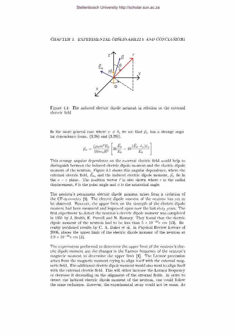
In the more general case where ψ 6= 0, we see that ~pψ has a strange angu-lar dependence (eqns. (3.38) and (3.39)).

~pψ =ζµ0m

2E0

10πε0R3

[36~E0

E0− 49

( ~E0 · ex)exE0

]

This strange angular dependence on the external electric eld would help todistinguish between the induced electric dipole moment and the electric dipolemoment of the neutron. Figure 4.1 shows this angular dependence, where theexternal electric eld, ~E0, and the induced electric dipole moment, ~pψ lie inthe x − z plane. The position vector ~r is also shown where r is the radialdisplacement, θ is the polar angle and φ is the azimuthal angle.

The neutron's permanent electric dipole moment arises from a violation ofthe CP-symmetry [2]. The electric dipole moment of the neutron has yet tobe observed. However, the upper limit on the strength of the electric dipolemoment had been measured and improved upon over the last sixty years. Therst experiment to detect the neutron's electric dipole moment was completedin 1951 by J. Smith, E. Purcell and N. Ramsey. They found that the electricdipole moment of the neutron had to be less than 5 × 10−20e cm [13]. Re-cently published results by C. A. Baker et al. in Physical Review Letters of2006, places the upper limit of the electric dipole moment of the neutron at2.9× 10−26e cm [1].

The experiments preformed to determine the upper limit of the neutron's elec-tric dipole moment use the changes in the Larmor frequency of the neutron'smagnetic moment to determine the upper limit [1]. The Larmor precessionarises from the magnetic moment trying to align itself with the external mag-netic eld. The additional electric dipole moment would also want to align itselfwith the external electric eld. This will either increase the Larmor frequencyor decrease it depending on the alignment of the external elds. In order todetect the induced electric dipole moment of the neutron, one could followthe same technique. However, the experimental setup would not be same. As



stated previously, the strength of the external electric eld would need to be ofthe order E0 ≈ 107 V/m for the induced electric moment of the neutron to becomparable with the permanent electric dipole moment of the neutron. Thesetypes of electric eld strengths are, however, found in some crystals. Lettingthe neutrons pass through one of these crystals would be sucient to induce anelectric dipole moment. By applying an external magnetic eld, one should ob-serve the induced electric dipole moment as a change in the Larmor frequency.The observability of the induced electric dipole moment is also helped by thestrange angular dependence which would not be present in the electric dipolemoment of the neutron.

Another possible experimental setup is the one discussed by V. Fedorov etal in the paper "Measurement of the neutron electric dipole moment by crystaldiraction" [6]. With this setup, neutrons passing through a crystal undergo aspin rotation. This rotation is then detected and used to determine the electricdipole moment of the neutron.

4.2 Outlook

Apart from the experiment to look for these induced electric and magneticeld, there are many more congurations to be considered. The only congu-rations that have been considered so far were the magnetic or electric sourcesin external quasi-static elds. Future possibilities could include both electricand magnetic sources in quasi-static elds. However, this will only producemore complicated expressions for ~V1(~x) (eqn. (3.7)) and ~V2(~x) (eqn. (3.8)).

The other possible adaption that could be made, is to derive ~E(~x) and ~B(~x) us-ing time-dependant external elds. In other words, Maxwell's equations wouldtake on the more general form:

~∇ · ~D = j0 ~∇× ~E = −∂~B

∂t

~∇ · ~B = 0 ~∇× ~H = ~j +∂ ~D

∂t

This would make ~E(~x) and ~B(~x) more general.

4.3 Conclusion

We have seen so far that the Heisenberg-Euler Lagrangian implies some in-teresting interaction between classical electric and magnetic eld sources; andexternal quasi-static electric and magnetic elds [3]. This interaction leads tocorrection to the elds produces by the sources as well as new elds, in thecase of pure electric and pure magnetic sources. These changes to the eldsare represented by the induced elds ~E(~x) and ~B(~x):

~E(~x) =ζ

4πε20~∇x∫

d3y

|~x− ~y|~∇y ·

8FM ~DM +

14

cGM ~HM

~B(~x) =

ζ

4πε20~∇x∫

d3y

|~x− ~y|~∇y ×

−8

cFM ~HM + 14GM ~DM



If we consider a uniformly charged spherical shell as a source for an electricelds then we nd that the external quasi-static magnetic eld induces a mag-netic dipole moment in the shell. The correction to the electric eld producedby the charged spherical shell is found to be signicantly smaller than the elec-tric eld and will therefore be unobservable when detecting the electric eldstrength. However, the induced magnetic dipole moment is something new andshould be detectable for the right combination of the total surface charge Q,the radius of the spherical shell R and the strength of the external quasi-staticmagnetic eld B0. The magnetic dipole moment ~m is given by the expression:

~m =c2ζ

6πε20

Q2

R~B

Using a charged spherical shell of total charge Q = 0.3 × 10−9C and radiusR = 1mm in the presence of an external magnetic eld of strength B0 = 1T ,produces a magnetic dipole moment of strength |~m| ≈ 10−30Am2.

The second case that was considered was a spherical shell with a current~j = 3|~m|

4πR3 δ(r − R)eφ moving on the surface of the shell. For distances greater

than the radius of the shell, R, the magnetic eld produced by the current ~jis the same as the magnetic eld produced by the magnetic dipole moment~m. An external quasi-static electric eld is applied over the shell and leads tothe production of the induced elds. The correction to the magnetic eld pro-duced by the current ~j is small compared to the magnetic eld and can safelybe ignored. The induced electric eld has the same form as an electric dipole.However, this induced electric dipole moment has a strange dependence on theangle, ψ, between the magnetic dipole moment and the external quasi-staticelectric eld. The electric dipole moment ~pψ is given by:

~pψ =ζµ0m

2E0

10πε0R3

[36~E0

E0− 49

( ~E0 · ex)exE0

]

For the case where ~E0||~m, namely ψ = 0, ~pψ reduces to ~p:

~p =36ζµ0m

2E0

10πε0R3ez

These results are very exciting and should produce some interesting experi-mental results. As electric and magnetic eld strengths increase, so too doesthe observability of the induces electric and magnetic elds. Experimental se-tups are being devised to detect and measure these induced elds using presenttechnology. The future of this subject looks very promising with possible ex-periments on the line as well as possible adaptions to the derivation of theinduced elds ~E(~x) and ~B(~x).


Bibliography

[1] C. A. Baker, D. D. Doyle, P. Geltenbort, K. Green, M. G. D. van derGrinten, P. G. Harris, P. Iaydjiev, S. N. Ivanov, D. J. R. May, J. M.Pendlebury, J. D. Richardson, D. Shiers, and K. F. Smith. Improvedexperimental limit on the electric dipole moment of the neutron. Phys.

Rev. Lett., 97(13):131801, Sep 2006.

[2] Shahida Dar. The Neutron EDM in the SM : A Review. arXiv:hep-ph/0008248v2, Aug 2000.

[3] C. A. Dominguez, H. Falomir, M. Ipinza, S. Kohler, M. Loewe, and J. C.Rojas. Qed vacuum uctuations and induced electric dipole moment ofthe neutron. Phys. Rev. D, 80(3):033008, Aug 2009.

[4] C. A. Dominguez, H. Falomir, M. Ipinza, M. Loewe, and J. C. Rojas.Induced electromagnetic elds in nonlinear qed. Modern Physics Letters

A, 24(23):18571862, Jul 2009.

[5] Gerald V. Dunne. Heisenber-euler eective lagrangians : Basics and ex-tensions. arXiv:hep-th/0406216v1, Jun 2004.

[6] V. V. Fedorov, M. Jentschel, I. A. Kuznetsov, E. G. Lapin,E. Lelievre-Berna, V. Nesvizhevsky, A. Petoukhov, S. Yu. Semenikhin,T. Soldner, F. Tasset, V. V. Voronin, and Yu. P. Braginetz. Mea-surement of the neutron electric dipole moment by crystal diraction.arXive:0907.1153v2[nucl-ex], Jul 2009.

[7] David J. Griths. Introduction to Electrodynamics, page 326. PrenticeHall International, Inc., 2003.

[8] David J. Griths. Introduction to Electrodynamics, page 58. Prentice HallInternational, Inc., 2003.

[9] David J. Griths. Introduction to Electrodynamics, pages 555557. Pren-tice Hall International, Inc., 2003.

[10] David J. Griths. Introduction to Quantum Mechanics, page 139. PearsonEducation, Limited, 2005.

[11] V. P. Gusynin and I. A. Shovkovy. Derivative expansion of the eectiveaction for qed in 2+1 and 3+1 dimensions. arXiv:hep-th/9804143v4, Jul1999.

[12] W. Heisenberg and H. Euler. Consequences of Dirac's theory of thepositron. arXiv:physics/0605038v1v1 [physics.hist-ph], May 2006.

34


BIBLIOGRAPHY 35

[13] J. H. Smith, E. M. Purcell, and N. F. Ramsey. Experimental limit to theelectric dipole moment of the neutron. Phys. Rev., 108(1):120122, Oct1957.


kohler, shane jerome

Documents