kriging is well-suited to parallelize optimizationkriging is well-suited to parallelize optimization...

Kriging is well-suited to parallelize optimization

David Ginsbourger Rodolphe Le Riche and Laurent Carraro

1 Introduction

11 Motivations efficient optimization algorithms for expensive computer experiments

Beyond both estalished frameworks of derivative-based descent and stochastic search algorithms the riseof expensive optimization problems creates the need for newspecific approaches and procedures The wordrdquoexpensiverdquo mdashwhich refers to price andor time issuesmdash implies severely restricted budgets in terms ofobjective function evaluations Such limitations contrast with the computational burden typically associatedwith stochastic search techniques like genetic algorithms Furthermore the latter evaluations provide nodifferential information in a majority of expensive optimization problems whether the objective functionoriginate from physical or from simulated experiments Hence there exists a strong motivation for devel-oping derivative-free algorithms with a particular focuson their optimization performances in a drasticallylimited number of evaluations Investigating and implementing adequate strategies constitute a contemporarychallenge at the interface between Applied Mathematics andComputational Intelligence especially when itcomes to reducing optimization durations by efficiently taking advantage of parallel computation facilities

The primary aim of this chapter is to address parallelization issues for the optimization of expensive-to-evaluate simulators such as increasingly encountered in engineering applications like car crash tests nu-clear safety or reservoir forecasting More specificallythe work presented here takes place in the frame ofmetamodel-based design of computer experiments in the sense of [42] Even though the results and discus-sions might be extended to a more general scope we restrict ourself here for clarity to single-objective opti-

David GinsbourgerDepartement 3MI Ecole Nationale Superieure des Mines 158 cours Fauriel Saint-Etienne Francee-mailginsbourgeremsefr

Rodolphe Le RicheCNRS (UMR 5146) and Departement 3MI Ecole Nationale Superieure des Mines 158 cours Fauriel Saint-Etienne Francee-maillericheemsefr

Laurent CarraroDepartement 3MI Ecole Nationale Superieure des Mines 158 cours Fauriel Saint-Etienne Francee-mailcarraroemsefr

1

2 David Ginsbourger Rodolphe Le Riche and Laurent Carraro

mization problems for deterministic codes The simulator is seen as black-box functiony with d-dimensionalvector of inputs and scalar output the latter being often obtained as combination of several responsesMeta-models also calledsurrogate models are simplified representations ofy They can be used for predictingvalues ofy outside the initial design or visualizing the influence of each variable ony [27 43] They may alsoguide further sampling decisions for various purposes such as refining the exploration of the input space inpreferential zones or optimizing the functiony [22] Classical surrogates include radial basis functions[37]interpolation splines [52] neural nets [8] (deterministicmetamodels) or linear and non-linear regression[2] and Kriging [7] (probabilistic metamodels) We concentrate here on the advantages of probabilisticmetamodels for parallel exploration and optimization with a particular focus on the virtues of Kriging

12 Where Computational Intelligence and Kriging meet

Computational intelligence (CI) methods share in variousproportions four features

An history going from experiments to theory CI methods very often originate from empirical comput-ing experiments in particular from experiments that mimick natural processes (eg neural networks [4]ant colony optimization [5] simulated annealing [25]) Later on as researchers use and analyze themtheory develops and their mathematical content grows A good example is provided by the evolutionaryalgorithms [9] which have progressively mixed the genetic metaphor and stochastic optimization theory

An indirect problem representation In standard evolutionary optimization methods knowledgeaboutthe cost function takes the indirect form of a set of well-performing points known as ldquocurrent populationrdquoSuch set of points is an implicit partial representation of a function In fuzzy methods the probabilitydensity functions of the uncertain variables are averaged out Such indirect representations enable to workwith few mathematical assumptions and have broadened the range of applicability of CI methods

Parallelized decision process Most CI approaches are inherently parallel For example the evolution-ary or particle swarm optimization [24] methods process sets of points in parallel Neural networks havea internal parallel structure Today parallelism is crucial for taking advantage of the increasingly dis-tributed computing capacity The parallel decision makingpossibilities are related to the indirect problemrepresentations (through set of points distributions) and to the use of randomness in the decision process

Heuristics Implicit problem representations and the empirical genesis of the CI methods rarely allowmathematical proofs of the methods properties Most CI methods are thusheuristics

Kriging has recently gained popularity among several research communities related to CI ranging fromData Mining[16] andBayesian Statistics[34 48] toMachine Learning[39] where it is linked toGaussianProcess Regression[53] andKernel Method[12] Recent works [17 30 31] illustrate the practical relevanceof Kriging to approximate computer codes in application areas such as aerospace engineering or materialsscience Indeed probabilistic metamodels like Kriging seem to be particularly adapted for the optimizationof black-box functions as analyzed and illustrated in the excellent article [20] The current Chapter is de-voted to the optimization of black-box functions using a kriging metamodel [14 22 49 51] Let us nowstress some essential relationships between Kriging and CIby revisiting the above list of features

A history from field studies to mathematical statistics Kriging comes from the earth sciences [29 33]and has been progressively developed since the 1950rsquos alongwith the discipline calledgeostatistics[2332] Originally aimed at estimating natural ressources in mining applications it has later been adaptedto address very general interpolation and approximation problems [42 43] The word ldquokrigingrdquo comes

Kriging is well-suited to parallelize optimization 3

from the name of a mining engineer Prof Daniel G Krige whowas a pioneer in the application ofmathematical statistics to the study of new gold mines usinga limited number of boreholes [29]

An indirect representation of the problem As will be detailed later in the text the kriging metamodelhas a powerful interpretation in terms of stochastic process conditionned by observed data points Theoptimized functions are thus indirectly represented by stochastic processes

Parallelized decision process The central contribution of this chapter is to propose toolsenabling paral-lelized versions of state-of-the art kriging-based optimization algorithms

Heuristics Although the methods discussed here are mathematically founded on the multipoints expectedimprovement the maximization of this criterion is not mathematically tractable beyond a few dimensionsIn the last part of the chapter it is replaced by the ldquokrigingbelieverrdquo and the ldquoconstant liarrdquo heuristics

Through their indirect problem representation their parallelism and their heuristical nature the kriging-based optimization methods presented hereafter are Computational Intelligence methods

13 Towards Kriging-based parallel optimization summary of obtained results andoutline of the chapter

This chapter is a follow-up to [14] It proposes metamodel-based optimization criteria and related algorithmsthat are well-suited to parallelization since they yield several points at each iteration The simulations asso-ciated with these points can be distributed on different processors which helps performing the optimizationwhen the simulations are calculation intensive The algorithms are derived from a multi-points optimizationcriterion themulti-pointsor q-points expected improvement(q-EI) In particular an analytic expression isderived for the 2-EI and consistent statistical estimatesrelying on Monte-Carlo methods are provided forthe general case All calculations are performed in the framework of Gaussian processes (GP) Two classesof heuristic strategies theKriging Believer(KB ) andConstant Liar(CL ) are subsequently introduced toobtain approximatelyq-EI-optimal designs The latter strategies are tested and compared on a classical testcase where theConstant Liarappears to constitute a legitimate heuristic optimizer of the q-EI criterionWithout too much loss of generality the probabilistic metamodel considered is Ordinary Kriging (OK seeeqs 1235) like in the founder work [22] introducing the now famousEGO algorithm In order to make thisdocument self-contained non-specialist readers may find an overview of existing criteria for kriging-basedsequential optimization in the next pages as well as a shortbut dense introduction to GP and OK in the bodyof the chapter with complements in appendix The outline ofthe chapter is as follows

bull Section 2 (Background in Kriging for Sequential Optimization) recalls the OK equations with a focuson the joint conditional distributions associated with this probabilistic metamodel A progressive in-troduction to kriging-based criteria for sequential optimization is then proposed culminating with thepresentation of the EGO algorithm and its obvious limitations in a context of distributed computing

bull Section 3 (The Multi-points Expected Improvement) consists in the presentation of theq-EI criterion mdashcontinuing the work initiated in [47]mdash its explicit calculation whenq= 2 and the derivation of estimatesof the latter criterion in the general case relying on Monte-Carlo simulations of gaussian vectors

bull Section 4 (Approximated q-EI maximization) introduces two heuristic strategies KB and CL to circum-vent the computational complexity of a directq-EI maximization These strategies are tested on a classicaltest-case and CL is found to be a very promizing competitor for approximatedq-EI maximization


bull Section 5 (Towards Kriging-based Parallel Optimization Conclusionand Perspectives) gives a summaryof obtained results as well as some related practical recommendations and finally suggests what theauthors think are perspectives of research to address the most urgently in order to extend this work

bull The appendix 6 is a short but dense introduction to GP for machine learning with an emphasis on thefoundations of both Simple Kriging and Ordinary Kriging by GP conditionning

Some notations y xisinDsubRdrarr y(x)isinR refers to the objective function wheredisinN0 is the numberof input variables andD is the set in which the inputs vary most of the time assumed tobe a compact andconnex1 subset ofRd At first y is known at aDesign of ExperimentsX = x1 xn wherenisin N is thenumber of initial runs or experiments and eachxi (1le i le n) is hence ad-dimensional vector(xi

1 xid)

We denote byY = y(x1) y(xn) the set of observations made by evaluatingy at the points ofX Thedata(XY) provides information on which is initially based the metamodeling ofy with an accuracy thatdepends onn the geometry ofX and the regularity ofy The OK mean predictor and prediction varianceare denoted by the functionsmOK() ands2

OK() The random process implicitely underlying OK is denotedby Y() in accordance with the notations of eq (35) presented in appendix The symbol rdquo|rdquo is used forconditioning together with the classical symbols for probability and expectation respectivelyP andE

2 Background in Kriging for Sequential Optimization

21 The Ordinary Kriging metamodel and its Gaussian Process interpretation

OK is the most popular Kriging metamodel simultaneously due to its great versatility and applicability Itprovides a mean predictor of spatial phenomena with a quantification of the expected prediction accuracyat each site A full derivation of the OK mean predictor and variance in a GP setting is proposed in theappendix The corresponding OK mean and variance functionsare given by the following formulae

mOK(x) =

[

c(x)+

(

1minusc(x)TΣminus11n

1Tn Σminus11n

)

1n

]T

Σminus1Y (1)

s2OK(x) = σ2minusc(x)TΣminus1c(x)+

(1minus1Tn Σminus1c(x))2

1Tn Σminus11n

(2)

wherec(x) =(

c(Y(x)Y(x1)) c(Y(x)Y(xn)))T

andΣ andσ2 are defined following the assumptions2

and notations given in appendix 6 Classical properties of OK include thatforalli isin [1n] mOK(xi) = y(xi) ands2OK(xi) = 0 therefore[Y(x)|Y(X) = Y] is interpolating Note that[Y(xa)|Y(X) = Y] and[Y(xb)|Y(X) = Y]

are dependent random variables wherexa andxb are arbitrary points of D as we will develop later

The OK metamodel of the Branin-Hoo function (Cf eq 25) is plotted on fig 21 The OK interpolation(upper middle) is based only on 9 observations Even if the shape is reasonably respected (lower middle)

1 Connexity is sometimes untenable in practical applications seeeg [46] for a treatment of disconnected feasible regions2 An extension to covariance non-stationary processes [35] is straightforward but beyond the scope of the present work


Fig 1 Ordinary Kriging of the Branin-Hoo function (function Kriging mean value and variance from left to right) The designof experiments is a 3times3 factorial design The covariance is an anisotropic squared exponential with parameters estimated bygaussian likelihood maximization [7]

the contour of the mean shows an artificial optimal zone (upper middle around the point(62)) In otherrespects the variance is not depending on the observations3 (eq 2) Note its particular shape due to theanisotropy of the covariance kernel estimated by likelihood maximization In modern interpretations [39]deriving OK equations is often based on the assumption thaty is a realization of a random process Y withunknown constant mean and known covariance (see [1] or [12] for a review of classical covariance kernels)Here we follow the derivation of 64 which has the advantageof delivering a gaussian posterior distribution

[Y(x)|Y(X) = Y]simN (mOK(x)s2OK(x)) (3)

Note that both a structure selection and a parametric estimation are made in practice one often chooses ageneralized exponential kernel with plugged-in maximum likelihood covariance hyperparameters ie with-out taking the estimation variance into account [22] This issue is sometimes addressed using a full bayesiantreatment as can be found in [43] or more recently in [15 34 39] Rephrasing 3 under the latter GP as-

3 phenomenon known as homoskedasticity of the Kriging variance with respect to the observations [7]


sumptions the random variableY(x) knowing the values ofy(x1) y(xn) follows a gaussian distributionwhich mean and variance are respectivelyE[Y(x)|Y(X) = Y] = mOK(x) andVar[Y(x)|Y(X) = Y] = s2

OK(x)In fact as shown in appendix (Cf eq 38) one can even get much more than these marginal conditionaldistributionsY()|Y(X) = Y constitutes a random process which is itself gaussian and as such completelycharacterized by its conditional meanmOK and conditional covariance kernelcOK explicited herunder

[Y()|Y(X) = Y]simGP(mOK()cOK( )) (4)

wherecOK(xxprime) = c(xminusxprime)minusc(x)TΣminus1c(xprime)+σ2[

(1minus1Tn Σminus1c(x))(1minus1T

n Σminus1c(xprime))1T

n Σminus11n

]

(5)

This new kernelcOK is not stationary even ifc is In other respects the knowledge ofmOK andcOK is the firststep to performing conditional simulations ofY knowing the observationsY(X) = Y which is easily feasibleat any new finite design of experiments whatever the dimension of inputs This will enable the computationof any multi-points sampling criterion such as proposed inthe forthcoming section about parallelization

22 Kriging-based optimization criteria

GP metamodels [39 53] such as OK has been used for optimization (minimization by default) There is adetailed review of optimization methods relying on a metamodel in [44 45] or [20] The latter analyzes whydirectly optimizing a deterministic metamodel (like a spline a polynomial or the kriging mean) is dangerousand does not even necessarily lead to a local optimum Kriging-based sequential optimization strategies (asdeveloped in [22] and commented in [20]) address the issue of converging to non (locally) optimal pointsby taking the kriging variance term into account (hence encouraging the algorithms to explore outside thealready visited zones) Such algorithms produce one point at each iteration that maximizes a figure of meritbased upon[Y(x)|Y(X) = Y] In essence the criteria balance kriging mean prediction and uncertainty

221 Visiting the point with most promizing mean minizingmOK

When approximatingy by mOK it might seem natural to hope that minimizingmOK instead ofy bringssatisfying results However a function and its approximation (mOK or other) can show substantial differencesin terms of optimal values and optimizers More specifically depending on the kind of covariance kernel usedin OK the minimizer ofmOK is susceptible to lie at (or near to) the design point with minimal y value Takingthe geometry of the design of experiments and space-filling considerations into account within explorationcriteria then makes sense The Kriging variance can be of providential help for this purpose

222 Visiting the point with highest uncertainty maximizing sOK

A fundamental mistake of minimizingmOK is that no account is done of the uncertainty associated withitAt the extreme inverse it is possible to define the next optimization iterate as the least known point inD


xprime = argmaxxisinD sOK(x) (6)

This procedure defines a series ofxprimes which will fill the spaceD and hence ultimately locate a global opti-mum Yet since no use is made of previously obtainedY information mdashlook at formula 2 fors2

OKmdash thereis no bias in favor of high performance regions Maximizing the uncertainty is inefficient in practice

223 Compromizing betweenmOK and sOK

The most general formulation for compromizing between the exploitation of previous simulations broughtby mOK and the exploration based onsOK is the multicriteria problem

minxisinD mOK(x)maxxisinD sOK(x)

(7)

Let P denote the Pareto set of solutions4 Finding one (or many) elements inP remains a difficult problemsinceP typically contains an infinite number of points A comparable approach calleddirect although notbased on OK is described in [21] the metamodel is piecewiselinear and the uncertainty measure is adistance to already known points The spaceD is discretized and the Pareto optimal set defines areas wherediscretization is refined The method becomes computationally expensive as the number of iterations anddimensions increase Note that [3] proposes several parallelized versions ofdirect

224 Maximizing the probability of improvement

Among the numerous criteria presented in [20] the probability of getting an improvement of the functionwith respect to the past evaluations seems to be one of the most fundamental This function is defined forevery x isin D as the probability for the random variableY(x) to be below the currently known minimummin(Y) = miny(x1) y(xn) conditional on the observations at the design of experiments

PI(x) = P(Y(x)lemin(Y(X))|Y(X) = Y) (8)

= E[

1Y(x)lemin(Y(X))|Y(X) = Y]

= Φ(

min(Y)minusmOK(x)

sOK(x)

)

(9)

whereΦ is the gaussian cumulative distribution function and the last equality follows 3 The thresholdmin(Y) is sometimes replaced by some arbitrary targetT isin R as evokated in [38] PI is known to providea very local search whenever the value of T is equal or close tomin(Y) Taking severalT rsquos is a remedyproposed by [20] to force global exploration Of course this new degree of freedom is also one more pa-rameter to fit In other respects PI has also been succesfully used as pre-selection criterion in GP-assistedevolution strategies [49] where it was pointed out that PI is performant but has a tendency to sample in un-explored areas We argue that the chosen covariance structure plays a capital role in such matters dependingwhether the kriging mean is overshooting the observations or not The next presented criterion theexpectedimprovement is less sensitive to such issues since it explicitly integrates both kriging mean and variance

4 Definition of the Pareto front of (sOKminusmOK) forallx isinP∄ zisin D (mOK(z) lt mOK(x) andsOK(z) ge sOK(x)) or (mOK(z) lemOK(x) andsOK(z) gt sOK(x))


Fig 2 PI and EI surfaces of the Branin-Hoo function (same design of experiments Kriging model and covariance parametersas in fig (21)) Maximizing PI leads to sample near the good points (associated with low observations) whereas maximizingEI leads here to sample between the good points By constructionboth criteria are null at the design of experiments but theprobability of improvement is very close to12 in a neighborhood of the point(s) where the function takes itscurrent minimum

225 Maximizing the expected improvement

An alternative solution is to maximize theexpected improvement(EI)

EI(x) = E[(min(Y(X)minusY(x))+|Y(X) = Y] = E[max0min(Y(X)minusY(x)|Y(X) = Y] (10)

that additionally takes into account the magnitude of the improvements EI measures how much improvementis expected by sampling atx In fine the improvement will be 0 ify(x) is abovemin(Y) andmin(Y)minusy(x)else Knowing the conditional distribution ofY(x) it is straightforward to calculate EI in closed form

EI(x) = (min(Y)minusmOK(x))Φ(

min(Y)minusmOK(x)

sOK(x)

)

+sOK(x)φ(

min(Y)minusmOK(x)

sOK(x)

)

(11)


whereφ stands for the probability density function of the standardnormal lawN (01)

Proof of 11EI(x) = E[(min(Y)minusY(x)) Y(x)lemin(Y)|Y(X) = Y]

=int min(Y)

minusinfin(min(Y)minus t) f

N (mKO(x)s2KO(x))(t)dt =

int

min(Y)minusmKO(x)sKO(x)

minusinfin(min(Y)minusmKO(x)minussKO(x)timesu) fN (01)(u)du

= (min(Y)minusmKO(x))int


minusinfinfN (01)(u)duminussKO(x)

int


minusinfinutimes fN (01)(u)du

= (min(Y)minusmKO(x))Φ(

min(Y)minusmKO(x)

sKO(x)

)

+sKO(x)φ(

min(Y)minusmKO(x)

sKO(x)

)

EI represents a trade-off between promising and uncertain zones This criterion has important properties forsequential exploration it is null at the already visited sites and positive everywhere else with a magnitudethat is increasing with the Kriging variance and with the decreasing Kriging mean (EI maximizers are indeedpart of the Pareto front of (sOKminusmOK)) Such features are usually demanded from global optimizationprocedures (see [21] for instance) EI and the probability of improvement are compared in fig (2)

226 TheStepwise Uncertainty Reduction(SUR) strategy

SUR has been introduced in [11] and extended to global optimization in [50 51] By modelingy using theprocessYrsquos conditional lawY(x)|Y it is possible to definexlowast|Y the conditional law ofYrsquos global minimizerxlowast and its densitypxlowast|Y(x) The uncertainty about the location ofxlowast is measured as the entropy ofpxlowast|Y(x)H(xlowast|Y) H(xlowast|Y) diminishes as the distribution ofxlowast|Y gets more peaked Conceptually the SUR strategyfor global optimization chooses as next iterate the point that specifies the most the location of the optimum

xprime = argminxisinDH(xlowast|YY(x)) (12)

In practicepxlowast|Y(x) is estimated by Monte-Carlo sampling ofY(x)|Y at a finite number of locations inDwhich may become a problem in high dimensionalDrsquos as the number of locations must geometrically in-crease withd to properly fill the space The SUR criterion is different in nature from the criteria presentedso far in that it does not maximize an immediate (ie at the next iteration) payoff but rather lays the founda-tion of a delayed payoff by gaining a more global knowledge onY (reduce the entropy of its optima) Themulti-points EI criterion we are focusing on in the present chapter also uses a delayed payoff measure

227 TheEfficient Global Optimization(EGO) algorithm

EGO [22] relies on the EI criterion Starting with an initialDesignX (typically a Latin Hypercube) EGOsequentially visits the current global maximizer of EI (saythe first visited one if there is more than one globalmaximizer) and updates the OK metamodel at each iteration including hyperparameters re-estimation

1 Evaluate y at X set Y = y(X) and estimate covariance parameters of Y byMLE (Maximum Likelihood Estimation)

2 While stopping criterion not met

a Compute xprime = argmaxxisinDEI(x) set X = Xcupxprime and Y = Ycupy(xprime)b Re-estimate covariance parameters by MLE


After having been developed in [22 47] EGO has inspired contemporary works in optimization ofexpensive-to-evaluate functions For instance [19] exposes some EGO-based methods for the optimiza-tion of noisy black-box functions like stochastic simulators [18] focuses on multiple numerical simulatorswith different levels of fidelity and introduces the so-calledaugmented EIcriterion integrating possible het-erogeneity in the simulation times Moreover [26] proposes an adaptation to multi-objective optimization[17] proposes an original multi-objective adaptation of EGO for physical experiments and [28] focuses onrobust criteria for multiobjective constrained optimization with applications to laminating processes

In all one major drawback of the EGO-like algorithms discussed so far is that they do not allow parallelevaluations ofy which is desirable for costly simulators (eg a crash-test simulation run typically lasts 24hours) This was already pointed out in [47] where the multi-points EI was defined but not further developedHere we continue this work by expliciting the latter multi-points EI (q-EI) and by proposing two classesof heuristics strategies meant to approximatly optimize the q-EI and hence (almost) simultaneously deliveran arbitrary number of points without intermediate evaluations of y In particular we analytically derivethe 2-EI and explain in detail how to take advantage of statistical interpretations of Kriging to consistentlycomputeq-EI by simulation whenq gt 2 which happens to provide quite a general template for desigingKriging-based parallel evaluation strategies dedicated to optimization or other purposes

3 The Multi-points Expected Improvement (q-EI) Criterion

The main objective of the present work is to analyze and then approximately optimize a global optimizationcriterion theq-EI that yieldsq points Sinceq-EI is an extension of EI all derivations are performed withinthe framework of OK Such criterion is the first step towards aparallelized version of the EGO algorithm[22] It also departs like the SUR criterion from other criteria that look for an immediate payoff We nowpropose a progressive construction of theq-EI by coming back to the random variableimprovement

Both criteria of PI and EI that we have previously recalled share indeed the feature of being conditionalexpectations of quantities involving theimprovement Theimprovementbrought by sampling at somex isin Dis indeed defined byI(x) = (min(Y(X))minusY(x))+ and is positive whenever the value sampled atx Y(x)is below the current minimummin(Y(X)) Now if we sampleY at q new locationsxn+1 xn+q isin Dsimultaneously it seems quite natural to define the joint mdashormultipointsmdash improvement as follows

forallxn+1 xn+q isin D I(xn+1

xn+q) = max(

I(xn+1) I(xn+q))

= max(

(min(Y(X))minusY(xn+1))+ (min(Y(X))minusY(xn+q))+)

=(

min(Y(X))minusmin(Y(xn+1) Y(xn+q)))+

(13)

where we used the fact thatforallabcisinR max((aminusb)+(aminusc)+) = (aminusb)+ if ble c and(aminusc)+ else Theway of unifying theq criteria of (1-point) improvements used in eq 13 deserves to be calledelitist one jugesthe quality of the set ofq-points as a function only of the one that performs the best This is to be comparedfor instance to the weighted sums of criteria encountered inmany political science applications

The q-points EI criterion (as already defined but not developed in [47] under the name rdquoq-step EIrdquo) is thenstraightforwardly defined as conditional expectation of the improvement brought by the q considered points


EI(xn+1 xn+q) = E[max(min(Y(X))minusY(xn+1))+ (min(Y)minusY(xn+q))+|Y(X) = Y]

= E[

(min(Y(X))minusmin(

Y(xn+1) Y(xn+q))

)+|Y(X) = Y]

= E[

(min(Y)minusmin(

Y(xn+1) Y(xn+q))

)+|Y(X) = Y]

(14)

Hence theq-EI may be seen as the regular EI applied to the random variable min(Y(xn+1) Y(xn+q)) Wethus have to deal with a minimum of dependent random variables Fortunately eq 4 provides us with theexact joint distribution of the q unknown responses conditional on the observations

[(Y(xn+1) Y(xn+q))|Y(X) = Y]simN ((mOK(xn+1) mOK(xn+q))Sq) (15)

where the elements of the conditional covariance matrixSq are(Sq)i j = cOK(xn+i xn+ j) (See eq 5) We nowpropose two different ways to evaluate the criterion eq 14depending whetherq = 2 orqge 3

31 Analytical calculation of 2-EI

Fig 3 1-EI (lower left) and 2-EI (right) functions associated with amonodimensional quadratic function (y(x) = 4times(xminus045)2

known atX = minus1minus050051 The OK metamodel has here a cubic covariance with parametersσ2 = 10 scale= 09)


We first focus on the calculation of the 2-EI associated with two arbitrary pointsxn+1xn+2 isin D defined as

EI(xn+1xn+2) = E[(min(Y(X))minusmin(Y(xn+1)Y(xn+2)))+|Y(X) = Y]

Let us remark that in reformulating the positive part function the expression above can also be written

EI(xn+1xn+2) = E[(min(Y(X))minusmin(Y(xn+1)Y(xn+2)))1min(Y(xn+1)Y(xn+2))lemin(Y)|Y(X) = Y]

We will now show that the 2-EI can be developed as a sum of two 1-EIrsquos plus a correction term involving1- and 2-dimensional gaussian cumulative distributions

Before all some classical results of conditional calculusallow us to precise the dependence betweenY(xn+1)andY(xn+2) conditional onY(X) = Y and to fix some additional notationsforalli j isin 12 (i 6= j) we note

mi = mKO(xi) = E[Y(xn+i)|Y(X) = Y]

σi = sKO(xn+i) =radic

Var[Y(xn+i)|Y(X) = Y]

c12 = ρ12σ1σ2 = cov[Y(xn+1)Y(xn+2)|Y(X) = Y]

mi| j = E[Y(xn+i)|Y(X) = YY(xn+ j))] = mi +c12σminus2i (Y(xn+ j)minusmj)

σ2i| j = σ2

i minusc12σminus2j = σ2

i (1minusρ212)

(16)

At this stage we are in position to computeEI(xn+1xn+2) in four steps From now on we replace the com-plete notationY(xn+i) by Yi and forget the conditioning onY(X) = Y for the sake of clarity

Step 1

EI(xn+1xn+2) = E[(min(Y)minusmin(Y1Y2))1min(Y1Y2)lemin(Y)]

= E[(min(Y)minusmin(Y1Y2))1min(Y1Y2)lemin(Y)(1Y1leY2 +1Y2leY1)]

= E[(min(Y)minusY1)1Y1lemin(Y)1Y1leY2 ]+E[(min(Y)minusY2)1Y2lemin(Y)1Y2leY1]

Since both terms of the last sum are similar (up to a permutation betweenxn+1 andxn+2) we will restrictour attention to the first one Using1Y1leY2 = 1minus1Y2leY1

5 we get

E[(min(Y)minusY1)1Y1lemin(Y)1Y1leY2 ] = E[(min(Y)minusY1)1Y1lemin(Y)(1minus1Y2leY1)]

= EI(xn+1)minusE[(min(Y)minusY1)1Y1lemin(Y)1Y2leY1]

= EI(xn+1)+B(xn+1xn+2)

whereB(xn+1xn+2) = E[(Y1minusmin(Y))1Y1lemin(Y)1Y2leY1] Informally B(xn+1xn+2) is the opposite of theimprovement brought byY1 whenY2 le Y1 and hence that doesnrsquot contribute to the 2-points improvementOur aim in the next steps will be to give an explicit expression for B(xn+1xn+2)

Step 2

5 This expression should be noted 1minus1Y2ltY1 but since we work with continous random variables it sufficiesthat their correla-tion is 6= 1 for the expression to be exact (Y1 = Y2) is then neglectable) We implicitely do this assumption in the following


B(xn+1xn+2) = E[Y11Y1lemin(Y)1Y2leY1 ]minusmin(Y)E[1Y1lemin(Y)1Y2leY1]

At this point it is worth noticing thatY1L= m1+σ1N1 (always conditional onY(X) = Y) with N1simN (01)

Substituing this decomposition in the last expression ofB(xn+1xn+2) delivers

B(xn+1xn+2) = σ1E[N11Y1lemin(Y)1Y2leY1]+ (m1minusmin(Y))E[1Y1lemin(Y)1Y2leY1 ]

The two terms of this sum require some attention We compute them in detail in the two next steps

Step 3 Using a key property of conditional calculus6 we obtain

E[N11Y1lemin(Y)1Y2leY1 ] = E[N11Y1lemin(Y)E[1Y2leY1|Y1]]

and the fact thatY2|Y1simN (m2|1(Y1)s22|1(Y1)) (all conditional on the observations) leads to the following

E[1Y2leY1|Y1] = Φ(

Y1minusm2|1s2|1

)

= Φ

Y1minusm2minus c12

σ21

(Y1minusm1)

σ2

radic

1minusρ212

Back to the main term and using again the normal decomposition of Y1 we get

E[

N11Y1lemin(Y)1Y2leY1

]

=

N11N1le

min(Y)minusm1σ1

Φ

m1minusm2 +(σ1minusρ12σ2)N1

σ2

radic

1minusρ212

= E[

N11N1leγ1Φ(α1N1 +β1)]

whereγ1 =min(Y)minusm1

σ1 β1 =

m1minusm2

σ2

radic

1minusρ212

andα1 =σ1minusρ12σ2

σ2

radic

1minusρ212

(17)

E[N11N1leγ1Φ(α1N1 +β1)] can be computed applying an integration by parts

int γ1

minusinfinuφ(u)Φ(α1u+β1)du=minusφ(γ1)Φ(α1γ1 +β1)+

α1

2π

int γ1

minusinfineminusu2minus(α1u+β1)2

2 du

And sinceu2 +(α1u+β1)2 =

(

radic

(1+α21)u+ α1β1radic

1+α21

)2

+β 2

11+α2

1 the last integral reduces to

radic2πφ

(radic

β 21

1+α21

)

int γ1

minusinfine

minus

radic(1+α2

1 )u+α1β1radic

1+α21

2

2 du=

2πφ(radic

β 21

1+α21

)

radic

(1+α21)

int

radic(1+α2

1)γ1+α1β1radic

1+α21

minusinfin

eminusv2

2radic

2πdv

We conclude in using the definition of the cumulative distribution function

6 For all functionφ in L 2(RR) E[Xφ(Y)] = E[E[X|Y]φ(Y)]


E[N11Y1lemin(Y)1Y2leY1] =minusφ(γ1)Φ(α1γ1 +β1)+

α1φ(radic

β 21

1+α21

)

radic

(1+α21)

Φ

radic

(1+α21)γ1 +

α1β1radic

1+α21

Step 4 We then compute the termE[1Y1lemin(Y)1Y2leY1] = E[1Xlemin(Y)1Zle0] where(XZ) = (Y1Y2minusY1) fol-lows a 2-dimensional gaussian distribution with expectationM = (m1m2minusm1) and covariance matrixΓ =(

σ21 c12minusσ2

1c12minusσ2

1 σ22 +σ2

1 minus2c12

)

The final results rely on the fact thatE[1Xlemin(Y)1Zle0] =CDF(MΓ )(min(Y)0)

where CDF stands for the bi-gaussian cumulative distribution function

EI(x1x2) = EI(x1)+EI(x2)+B(x1

x2)+B(x2x1) (18)

where

B(x1x2) = (mOK(x1)minusmin(Y))δ (x1x2)+σOK(x1)ε(x1x2)

ε(x1x2) = α1φ(

|β1|radic(1+α2

1)

)

Φ(

(1+α21)

12

(

γ + α1β11+α2

1

))

minusφ(γ)Φ(α1γ +β1)

δ (x1x2) = CDF(Γ )

(

min(Y)minusm1

m1minusm2

)

Figure 31 represents the 1-EI and the 2-EI contour plots associated with a deterministic polynomial functionknown at 5 points 1-EI advises here to sample between the rdquogood pointsrdquo ofX The 2-EI contour illustratessome general properties 2-EI is symmetric and its diagonalequals 1-EI what can be easily seen by comingback to the definitions Roughly said 2-EI is high whenever the 2 points have high 1-EI and are reasonablydistant from another (precisely in the sense of the metric used in OK) Additionally maximizing 2-EI selectshere the two best local optima of 1-EI (x1 = 03 andx2 = 07) This is not a general fact The next exampleillustrates for instance how 2-EI maximization can yield two points located around (but different from) 1-EIrsquosglobal optimum whenever 1-EI has one single peak of great magnitude (see fig 4)

32 q-EI computation by Monte Carlo Simulations

Extrapolating the calculation of 2-EI to the general case gives complex expressions depending on q-dimensional gaussian cdfrsquos Hence it seems that the computation of q-EI when q is large would have torely on numerical multivariate integral approximation techniques anyway Therefore directly evaluating q-EI by Monte-Carlo Simulation makes sense Thanks to eq 15 the random vector(Y(xn+1) Y(xn+q)) canbe simulated conitional onY(X) = Y using a decomposition (eg Mahalanobis) of the covariancematrixSq

forallkisin [1nsim] Mk = (mOK(xn+1) mOK(xn+q))+ [S12q Nk]

TNk simN (0q Iq) iid (19)

Computing the conditional expectation of any function (notnecessarily linearly) of the conditioned randomvector(Y(xn+1) Y(xn+q)) knowingY(X) = Y can then be done in averaging the images of the simulated


Fig 4 1-point EI (lower left) and 2-points EI (right) functions associated with a monodimensional linear function (y(x) = 3timesx)known atX = minus1minus050051 The OK metamodel has here a cubic covariance with parametersσ2 = 10 scale= 14)

vectors by the considered function

1 function Q-EI(X Y Xnew)2 L = chol(Var[Y(Xnew)|Y(X) = Y]) ⊲ Decomposition ofSq (Cholesky Mahalanobis etc)3 for ilarr 1nsim do4 NsimN (0 Iq) ⊲ Drawing a standard gaussian vectorN at random5 Mi = mOK(Xnew)+LN ⊲ Simulating Y atXnew conditional onY(X) = Y6 qIsim(i)=[min(Y)minusmin(Mi)]

+ ⊲ Simulating the improvement atXnew

7 end for8 qEIsim = 1

nsimsumnsim

i=1 qIsim(i) ⊲ Estimation of theq-points Expected Improvement9 end function

A straightforward application of the Law of Large Numbers (LLN) yields indeed

qEIsim =nsim

sumi=1

[min(Y)minusmin(Mi)]+

nsimminusminusminusminusminusrarrnsimrarr+infin

EI(x1 xq) as (20)

and the Central Limit Theorem (CLT) can finally be used to control the precision of the Monte Carlo ap-proximation as a function ofnsim (see [40] for details concerning the variance estimation)


radicnsim

(

qEIsimminusEI(x1 xq)radic

Var[I(x1 xq)]

)

minusminusminusminusminusrarrnsimrarr+infin

N (01) in law (21)

4 Approximated q-EI maximization

The multi-points criterion that we have presented in the last section can potentially be used to deliver anadditional design of experiments in one step through the resolution of the optimization problem

(xprimen+1

xprimen+2

xprimen+q) = argmaxXprimeisinDq[EI(Xprime)] (22)

However the computation ofq-EI becomes intensive asq increases Moreover the optimization problem(22) is of dimensiondtimes q and with a noisy and derivative-free objective function inthe case where thecriterion is estimated by Monte-Carlo Here we try to find pseudo-sequential greedy strategies that approachthe result of problem 22 while avoiding its numerical cost hence circumventing the curse of dimensionality

41 A first greedy strategy to build a q-points design with the 1-point EI

Instead of searching for the globally optimal vector(xprimen+1x

primen+2 xprimen+q) an intuitive way of replacing it

by a sequential approach is the following first look for the next best single pointxn+1 = argmaxxisinDEI(x)then feed the model and look forxn+2 = argmaxxisinDEI(x) and so on Of course the valuey(xn+1) is notknown at the second step (else we would be in a real sequentialalgorithm like EGO) Nevertheless wedispose of two pieces of information the sitexn+1 is assumed to have already been visited at the previousiteration and[Y(xn+1)|Y = Y(X)] has a known distribution More precisely the latter is[Y(xn+1)|Y(X) =Y]simN (mOK(xn+1)s2

OK(xn+1)) Hence the second sitexn+2 can be computed as

xn+2 = argmaxxisinDE[

E[

(Y(x)minusmin(Y(X)))+|Y(X) = YY(xn+1)]]

(23)

and the same procedure can be applied iteratively to deliverq points computingforall j isin [1qminus1]

xn+ j+1 = argmaxxisinD

int

uisinR j

[

E[

(Y(x)minusmin(Y(X)))+|Y(X) = YY(xn+1) Y(xn+ jminus1)]]

fY(X1 j )|Y(X)=Y(u)du (24)

wherefY(X1 j )|Y(X)=Y is the multivariate gaussian density of the OK conditional distrubtion at(xn+1 xn+ j)Although eq 24 is a sequentialized version of the q-points expected improvement maximization it doesnrsquotcompletely fulfill our objectives There is still a multivariate gaussian density to integrate which seems tobe a typical curse in such problems dealing with dependent random vectors We now present two classes ofheuristic strategies meant to circumvent the computational complexity encountered in (24)


42 The Kriging Believer (KB) and Constant Liar (CL) strategies

Lying to escape intractable calculations starting from the principle of (24) we propose to weaken theconditional knowledge taken into account at each iteration This very elementary idea inspired two heuristicstrategies that we expose and test in the next two subsections theKriging Believerand theConstant Liar

421 Believing the OK predictor the KB heuristic strategy

The Kriging Believerstrategy replaces the conditional knowledge about the responses at the sites chosenwithin the last iterations by deterministic values equal tothe expectation of the kriging predictor Keepingthe same notations as previously the strategy can be summedup as follows

Algorithm 1 The Kriging Believer algorithm a first approximate solution of the multipoints problem(xprimen+1x

primen+2 xprimen+q) = argmaxXprimeisinDq[EI(Xprime)]

1 function KB(X Y q)2 for ilarr 1q do3 xn+i = argmaxxisinDEI(x)4 mOK(xn+i) = E[Y(xn+i)|Y(X) = Y]5 X = X

⋃xn+i6 Y = Y

⋃mOK(xn+i)7 end for8 end function

This sequential strategy delivers a q-points design and is computationally affordable since it relies on theanalytically known EI optimized ind dimensions However there is a risk of failure since believing an OKpredictor that overshoots the observed data may lead to a sequence that gets trapped in a non-optimal regionfor many iterations (see 43) We now propose a second strategy that reduces this risk

422 Updating the OK metamodel with fake observations theCL heuristic strategy

Let us now consider a sequential strategy in which the metamodel is updated (still without hyperparameterre-estimation) at each iteration with a valueL exogenously fixed by the user here called a rdquolierdquo The strategyreferred to as theConstant Liarconsists in lying with the same valueL at every iteration maximize EI (iefind xn+1) actualize the model as ify(xn+1) = L and so on always with the sameL isin RThe effect ofL on the performance of the resulting optimizer is investigated in the next sectionL shouldlogically be determined on the basis of the values taken byy at X Three valuesminY meanY andmaxY are considered here The largerL is the more explorative the algorithm will be and vice versa

43 Empirical comparisons with the Branin-Hoo function

The four optimization strategies presented in the last section are now compared on the the Branin-Hoofunction which is a classical test-case in global optimization [22 38 47]


Algorithm 2 The Constant Liar algorithm another approximate solutionof the multipoints problem(xprimen+1x


1 function CL(X Y L q)2 for ilarr 1q do3 xn+i = argmaxxisinDEI(x)4 X = X

⋃xn+i5 Y = Y

⋃L6 end for7 end function

yBH(x1x2) = (x2minus 514π2 x2

1 + 5π x1minus6)2 +10(1minus 1

8π )cos(x1)+10x1 isin [minus510] x2 isin [015]

(25)

yBH has three global minimizers(minus3141227) (314227) (942247) and the global minimum is ap-proximately equal to 04 The variables are normalized by the transformationx

prime1 = x1+5

15 andxprime2 = x2

15 Theinitial design of experiments is a 3times3 complete factorial designX9 (see 5 ) thusY = yBH(X9) OrdinaryKriging is applied with a stationary anisotropic gaussian covariance function

forallh = (h1h2) isin R2 c(h1h2) = σ2eminusθ1h2

1minusθ2h22 (26)

where the parameters (θ1θ2) are fixed to their Maximum Likelihood Estimate (527026) andσ2 is es-timated within kriging as an implicit function of (θ1θ2) (like in [22]) We build a 10-points optimizationdesign with each strategy and additionally estimated by Monte Carlo simulations (nsim = 104) the PI and EIvalues brought by theq first points of each strategy (hereqisin 2610) The results are gathered in Tab 43

Fig 5 (Left) contour of the Branin-Hoo function with the designX9 (small black points) and the 6 first points given by theheuristic strategy CL[min(yBH(X9))] (large bullets) (Right) Histogram of 104 Monte Carlo simulated values of the improve-ment brought by the 6-points CL[min(yBH(X9))] strategy The corresponding estimates of 6-points PI and EI aregiven above


The four strategies (KB and the three variants of CL) gave clearly different designs and optimization perfor-mances In the first caseConstant Liar(CL) sequences behaved as if the already visited points generateda repulsion with a magnitude increasing withL The tested valuesL = max(Y) andL = mean(Y) forcedthe exploration designs to fill the space by avoidingX9 Both strategies provided space-filling exploratorydesigns with high probabilities of improvement (10-PI near 100) and promising q-EI values (see Table 1)In fine they brought respective actual improvements of 786 and 625

Of all the tested strategies CL[min(Y)] gave here the best results In 6 iterations it visited the threelocally optimal zones ofyBH In 10 iterations it gave the best actual improvement amongthe consideredstrategies which is furthermore in agreement with the 10-points EI values simulated by Monte-Carlo Itseems in fact that the soft repulsion whenL = min(Y) is the right tuning for the optimization of the Branin-Hoo function with the initial designX9

In the second case the KB has yielded here disappointing results All the points (except one) were clusteredaround the first visited pointxn+1 (the same as inCL by construction) This can be explained by the exag-geratedly low prediction given by Kriging at this very point the mean predictor overshoots the data (becauseof the Gaussian covariance) and the expected improvement becomes abusively large in the neighborhoodof xn+1 Thenxn+2 is then chosen nearxn+1 and so on The algorithm gets temporarily trapped at the firstvisited point KB behaves in the same way asCL would do with a constantL below min(Y) As can beseen in Table 1 (last column) the phenomenon is visible on both the q-PI and q-EI criteria they remainalmost constant when q increases This illustrates in particular how q-points criteria can help in rejectingunappropriate strategies

CL[min(Y)] CL[mean(Y)] CL[max(Y)] KBPI (first 2 points) 877 87 889 65EI (first 2 points) 1143 114 1135 829PI (first 6 points) 946 955 927 655EI (first 6 points) 1174 1156 1151 852PI (first 10 points) 998 999 999 665EI (first 10 points) 1226 1184 117 8586

Improvement (first 6 points) 74 625 786 0Improvement (first 10 points) 837 625 786 0

Table 1 Multipoints PI EI and actual improvements for the 2 6 and 10first iterations of the heuristic strategies CL[min(Y)]CL[mean(Y)] CL[max(Y)] and Kriging Believer (here min(Y) = min(yBH(X9))) qminusPI andqminusEI are evaluated by Monte-Carlo simulations (Eq (20)nsim = 104)

In other respects the results shown in Tab 43 highlight a major drawback of the q-PI criterion Whenqincreases thePI associated with all 3 CL strategies quickly converges to 100 such that it is not possibleto discriminate between the good and the very good designs Theq-EI is a more selective measure thanks totaking the magnitude of possible improvements into account Nevertheless q-EI overevaluates the improve-ment associated with all designs considered here This effect (already pointed out in [47]) can be explainedby considering both the high value ofσ2 estimated fromY and the small difference between the minimalvalue reached atX9 (95) and the actual minimum ofyBH (04)We finally compared CL[min] CL[max] latin hypercubes (LHS) and uniform random designs (UNIF) interms ofq-EI values withq isin [110] For everyq isin [110] we sampled 2000q-elements designs of eachtype (LHS and UNIF) and compared the obtained empirical distributions ofq-points Expected Improvement


Fig 6 Comparaison of theq-EI associated with theq first points (q isin [110]) given by the constant liar strategies (min andmax) 2000q-points designs uniformly drawn for everyq and 2000q-points LHS designs taken at random for everyq

to theq-points Expected Improvement estimates associated with theq first points of both CL strategies

As can be seen on fig 6 CL[max] (light bullets) and CL[min] (dark squares) offer very goodq-EI resultscompared to random designs especially for small values ofq By definition the two of them start with the1-EI global maximizer which ensures aq-EI at least equal to 83 for allqge 1 Both associatedq-EI seriesthen seem to converge to threshold values almost reached for qge 2 by CL[max] (which dominates CL[min]whenq= 2 andq= 3) and forqge 4 by CL[min] (which dominates CL[max] for all 4le qle 10) The randomdesigns have less promizingq-EI expected values Theirq-EI distributions are quite dispersed which canbe seen for instance by looking at the 10minus 90 interpercentiles represented on fig 6 by thin full lines(respectively dark and light for UNIF and LHS designs) Notein particular that theq-EI distribution of theLHS designs seem globally better than the one of the uniform designs Interestingly the best designs everfound among the UNIF designs (dark dotted lines) and among the LHS designs (light dotted lines) almostmatch with CL[max] whenq isin 23 and CL[min] when 4le qle 10 We havenrsquot yet observed a designsampled at random that clearly provides betterq-EI values than the proposed heuristic strategies


5 Towards Kriging-based Parallel Optimization Conclusion and Perspectives

Optimization problems with objective functions steming from expensive computer simulations stronglymotivates the use of data-driven simplified mathematical representations of the simulator ormetamod-els An increasing number of optimization algorithms developed for such problems rely on metamodelscompeting with andor complementing population-based Computational Intelligence methods A repre-sentative example is given by the EGO algorithm [22] a sequential black-box optimization procedurewhich has gained popularity during the last decade and inspired numerous recent works in the field[10 17 18 19 20 26 28 36 44 50] EGO relies on a Kriging-based criterion the expected improvement(EI) accounting for the exploration-exploitation trade-off7 The latter algorithm unfortunately produces onlyone point at each iteration which prevents to take advantage of parallel computation facilities In the presentwork we came back to the interpretation of Kriging in terms of Gaussian Process[39] in order to propose aframework for Kriging-based parallel optimization and toprepare the work for parallel variants of EGO

The probabilistic nature of the Kriging metamodel allowed us to calculate the joint probability distributionassociated with the predictions at any set of points upon which we could rediscover (see [47]) and char-acterize a criterion named heremulti-points expected improvement or q-EI The q-EI criterion makes itpossible to get an evaluation of the rdquooptimization potentialrdquo given by any set of q new experiments Ananalytical derivation of 2-EI was performed providing a good example of how to manipulatejoint Krig-ing distributions for choosing additional designs of experiments and enabling us to shed more light on thenature of the q-EI thanks to selected figures For the computation of q-EI in the general case an alterna-tive computation method relying on Monte-Carlo simulations was proposed As pointed out in illustrated inthe chapter Monte-Carlo simulations offer indeed the opportunity to evaluate the q-EI associated with anygiven design of experiment whatever its sizen and whatever the dimension of inputsd However derivingq-EI-optimal designs on the basis of such estimates is not straightforward and crucially depending on bothn andd Hence some greedy alternative problems were considered four heuristic strategies the rdquoKrigingBelieverrdquo and three rdquoConstant Liarsrdquo have been proposed andcompared that aim at maximizing q-EI whilebeing numerically tractable It has been verified in the frame of a classical test case that theCL strategiesprovide q-EI vales comparable with the best Latin Hypercubes and uniformdesigns of experiments foundby simulation This simple application illustrated a central practical conclusion of this work consideringa set of candidate designs of experiments provided for instance by heuristic strategies it is always possi-ble mdashwhatevern anddmdash to evaluate and rank them using estimates of q-EI or related criteria thanks toconditional Monte-Carlo simulation

Perspectives include of course the development of synchronous parallel EGO variants delivering a set ofqpoints at each iteration The tools presented in the chaptermay constitute bricks of these algorithms as ithas very recently been illustrated on a succesful 6-dimensional test-case in the thesis [13] An R packagecovering that subject is in an advanced stage of preparationand should be released soon [41] On a longerterm the scope of the work presented in this chapter and notonly its modest original contributions couldbe broaden If the considered methods could seem essentially restricted to the Ordinary Kriging metamodeland concern the use of an optimization criterion meant to obtain q points in parallel several degrees offreedom can be played on in order to address more general problems First any probabilistic metamodelpotentially providing joint distributions could do well (regression models smoothing splines etc) Secondthe final goal of the new generated design might be to improve the global accuracy of the metamodel

7 Other computational intelligence optimizers eg evolutionary algorithms [9] address the explorationexploitation trade-offimplicitely through the choice of parameters such as the population size and the mutation probability


to learn a quantile to fill the space etc the work done here with the q-EI and associate strategies isjust a particular case of what one can do with the flexibility offered by probabilistic metamodels and allpossible decision-theoretic criteria To finish with two challenging issues of Computationnal Intelligencethe following perspectives seem particularly relevant at both sides of the interface with this work

bull CI methods are needed to maximize theq-EI criterion which inputs live in a(ntimesd)-dimensional spaceand which evaluation is noisy with tunable fidelity depending on the chosennsim values

bull q-EI and related criteria are now at disposal to help pre-selecting good points in metamodel-assistedevolution strategies in the flavour of [10]

AknowledgementsThis work was conducted within the frame of the DICE (Deep Inside Computer Exper-iments) Consortium between ARMINES Renault EDF IRSN ONERA and Total SA The authors wishto thank X Bay R T Haftka B Smarslok Y Richet O Roustant and V Picheny for their help and richcomments Special thanks to the R project people [6] for developing and spreading such a useful freewareDavid moved to Neuchatel University (Switzerland) for a postdoc and he gratefully thanks the MathematicsInstitute and the Hydrogeology Department for letting him spend time on the revision of the present chapter

6 Appendix

61 Gaussian Processes for Machine Learning

A real random process(Y(x))xisinD is defined as aGaussian Process(GP) whenever all its finite-dimensional distributionsare gaussian Consequently for allnisin N and for all setX = x1 xn of n points ofD there exists a vectorm isin Rn and asymmetric positive semi-definite matrixΣ isinMn(R) such that(Y(x1) Y(xn)) is a gaussian Vector following a multigaussianprobability distributionN (mΣ) More specifically for alli isin [1n] Y(xi) simN (E[Y(xi)]Var[Y(xi)]) whereE[Y(xi)] is theith coordinate ofm andVar[Y(xi)] is theith diagonal term ofΣ Furthermore all couples(Y(xi)Y(x j )) i j isin [1n] i 6= j aremultigaussian with a covarianceCov[Y(xi)Y(x j )] equal to the non-diagonal term ofΣ indexed byi and jA Random ProcessY is said to befirst order stationaryif its mean is a constant ie ifexistmicro isin R| forallx isin D E[Y(x)] = micro Yis said to besecond order stationaryif it is first order stationary and if there exists furthermore a function of positive typec DminusDminusrarrR such that for all pairs(xxprime) isinD2 Cov[Y(x)Y(xprime)] = c(xminusxprime) We then have the following expression for thecovariance matrix of the observations atX

Σ = (Cov[Y(xi)Y(x j )])i jisin[1n] = (c(xi minusx j ))i jisin[1n] =

σ2 c(x1minusx2) c(x1minusxn)c(x2minusx1) σ2 c(x2minusxn)

c(xnminusx1) c(xnminusx2) σ2

(27)

whereσ2 = c(0) Second order stationary processes are sometimes calledweakly stationary A major feature of GPs is thattheir weak stationarityis equivalent tostrong stationarity if Y is a weakly stationary GP the law of probability of the randomvariableY(x) doesnrsquot depend onx and the joint distribution of(Y(x1) Y(xn)) is the same as the distribution of(Y(x1 +h) Y(xn +h)) whatever the set of pointsx1 xn isinDn and the vectorh isinRn such thatx1 +h xn +h isinDn To sumup a stationary GP is entirely defined by its meanmicro and its covariance functionc() The classical framework of Kriging forComputer Experiments is to make predictions of a costly simulatory at a new set of sitesXnew= xn+1 xn+q (most of thetime q = 1) on the basis of the collected observations at the initial designX = x1 xn and under the assumption thatyis one realization of a stationary GPY with known covariance functionc (in theory) Simple Kriging (SK) assumes a knownmeanmicro isin R In Ordinary Kriging (OK)micro is estimated


62 Conditioning Gaussian Vectors

Let us consider a centered Gaussian vectorV = (V1V2) with covariance matrix

ΣV = E[VVT ] =

(

ΣV1 ΣTcross

Σcross ΣV2

)

(28)

Key properties of Gaussian vectors include that the orthogonal projection of a Gaussian vector onto a linear subspace is stilla Gaussian vector and that the orthogonality of two subvectorsV1V2 of a Gaussian vectorV (ie Σcross= E[V2VT

1 ] = 0) isequivalent to their independence We now express the conditional expectationE[V1|V2] E[V1|V2] is by definition such thatV1minusE[V1|V2] is independent ofV2 E[V1|V2] is thus fully characterized as orthogonal projection on thevector space spanned bythe components ofV2 solving the so callednormal equations

E[(V1minusE[V1|V2])VT2 ] = 0 (29)

Assuming linearity ofE[V1|V2] in V2 ie E[V1|V2] = AV2 (A isinMn(R)) a straightforward development of (eq29) gives thematrix equationΣT

cross= AΣV2 and henceΣTcrossΣminus1

V2V2 is a suitable solution providedΣV2 is full ranked8 We conclude that

E[V1|V2] = ΣTcrossΣminus1

V2V2 (30)

by uniqueness of the orthogonal projection onto a closed linear subspace in a Hilbert space Using the independence between(V1minusE[V1|V2]) andV2 one can calculate the conditional covariance matrixΣV1|V2

ΣV1|V2= E[(V1minusE[V1|V2])(V1minusE[V1|V2])

T |V2] = E[(V1minusAV2)(V1minusAV2)T ]

= ΣV1minusAΣcrossminusΣTcrossA

T +AΣV2AT = ΣV1minusΣTcrossΣminus1

V2Σcross

(31)

Now consider the case of a non-centered random vectorV = (V1V2) with meanm= (m1m2) The conditional distributionV1|V2can be obtained by coming back to the centered random vectorVminusm We then find thatE[V1minusm1|V2minusm2] = ΣT

crossΣminus1V2

(V2minusm2) and henceE[V1|V2] = m1 +ΣT

crossΣminus1V2

(V2minusm2)

63 Simple Kriging Equations

Let us come back to our metamodeling problem and assume thaty is one realization of a Gaussian ProcessY defined as follows

Y(x) = micro + ε(x)ε(x) centered stationary GP with covariance functionc()

(32)

wheremicro isin R is known Now say thatY has already been observed atn locationsX = x1 xn (Y(X) = Y) and that we wishto predictY aq new locationsXnew= xn+1 xn+q Since(Y(x1) Y(xn)Y(xn+1) Y(xn+q)) is a Gaussian Vector withmeanmicro1n+q and covariance matrix

Σtot =

(

Σ ΣTcross

Σcross Σnew

)

=

σ2 c(x1minusx2) c(x1minusxn+q)c(x2minusx1) σ2 c(x2minusxn+q)

c(xn+qminusx1) c(xn+qminusx2) σ2

(33)

We can directly apply eq (30) and eq (31) to derive the SimpleKriging Equations

[Y(Xnew)|Y(X) = Y]simN (mSK(Xnew)ΣSK(Xnew)) (34)

8 If ΣV2 is not invertible the equation holds in replacingΣminus1V2

by the pseudo-inverseΣdaggerV2


with mSK(Xnew) = E[Y(Xnew)|Y(X) = Y] = micro1q +ΣTcrossΣminus1(Yminusmicro1q) andΣSK(Xnew) = ΣnewminusΣT

crossΣminus1Σcross Whenq = 1Σcross= c(xn+1) = Cov[Y(xn+1)Y(X)] and the covariance matrix reduces tos2

SK(x) = σ2minus c(xn+1)TΣminus1c(xn+1) which iscalled theKriging Variance Whenmicro is constant but not known in advance it is not mathematically correct to sequentiallyestimatemicro and plug in the estimate in the Simple Kriging equations Ordinary Kriging addresses this issue

64 Ordinary Kriging Equations

Compared to Simple Kriging Ordinary Kriging (OK) is used when the mean of the underlying random process is constantand unknown We give here a derivation of OK in a Bayesian framework assuming thatmicro has an improper uniform priordistributionmicro simU (R) y is thus seen as a realization of a random processY defined as the sum ofmicro and a centered GP9


micro simU (R) (prior) independent ofε(35)

Note that conditioning with respect tomicro actually provides SK equations Lettingmicro vary we aim to find the law of[Y(Xnew)|Y(X) = Y] Starting with[Y(X) = Y|micro]simN (micro1nΣ) we getmicro rsquos posterior distribution

[micro|Y(X) = Y]simN(

microσ2micro)

= N

(

1TΣminus1Y1TΣminus11

1

1Tq Σminus11q

)

(posterior) (36)

We can re-write the SK equations[Y(Xnew)|Y(X) = Ymicro] simN (mSK(Xnew)ΣSK(Xnew)) Now it is very useful to notice thatthe random vector(Y(Xnew)micro) is Gaussian conditional onY(X) = Y 10 It follows that[Y(Xnew)|Y(X) = Y] is Gaussian andits mean and covariance matrix can finally be calculated with the help of classical conditional calculus results Hence usingmOK(Xnew) = E[Y(Xnew)|Y(X) = Y] = Emicro [E[Y(Xnew)|Y(X) = Ymicro]] we find thatmOK(Xnew) = micro + ΣT

crossΣminus1(Y minus micro1n)Similarly ΣOK(Xnew) can be obtained using thatCov[AB] = Cov[E[A|C]E[B|C]] + E[Cov[AB|C]] for all random variablesAB C such that all terms exist We then get for all couples of points(xn+i xn+ j ) (i j isin [1q])

Cov[Y(xn+i)Y(xn+ j )|Y(X) = Y]

=E[

Cov[Y(xn+i)Y(xn+ j )|Y(X) = Ymicro]]

+Cov[

E[Y(xn+i)|Y(X) = Ymicro]E[Y(xn+ j )|Y(X) = Ymicro]]

(37)

The left termCov[Y(xn+i)Y(xn+ j )|Y(X) = Ymicro] is the conditional covariance under the Simple Kriging Model The rightterm is the covariance betweenmicro + c(xn+i)TΣminus1(Yminus micro1q) andmicro + c(xn+ j)TΣminus1(Yminus micro1q) conditional on the observationsY(X) = Y Using eq 36 we finally obtain


=CovSK[Y(xn+i)Y(xn+ j )|Y(X) = Y]

+Cov[c(xn+i)TΣminus1(Y)+ micro(1+c(xn+i)TΣminus11q)c(xn+ j)TΣminus1(Y)+ micro(1+c(xn+ j)TΣminus11q)]

=c(xn+i minusxn+ j )minusc(xn+i)TΣminus1c(xn+ j )+(1+c(xn+i)TΣminus11q)(1+c(xn+ j)TΣminus11q)

1Tq Σminus11q

(38)

9 The resulting random processY is not Gaussian10 which can be proved by considering its Fourier transform


References

1 Abrahamsen P (1997) A review of gaussian random fields and correlation functions second editionTech Rep 917 Norwegian Computing Center Olso

2 Antoniadis A Berruyer J Carmona R (1992) Regression non lineaire et applications Economica Paris3 Baker C Watson LT Grossman B Mason WH Haftka RT (2001) Parallel global aircraft configuration

design space exploration Practical parallel computing pp79ndash964 Bishop C (1995) Neural Networks for Pattern RecognitionOxford Univ Press5 Blum C (2005) Ant colony optimization introduction and recent trends Physics of life review 2353ndash

3736 development Core Team R (2006) R A language and environment for statistical computing URL

httpwwwR-projectorg7 Cressie N (1993) Statistics for spatial data Wiley series in probability and mathematical statistics8 Dreyfus G Martinez JM (2002) Reseaux de neurones Eyrolles9 Eiben A Smith J (2003) Introduction to Evolutionary Computing Springer Verlag

10 Emmerich M Giannakoglou K Naujoks B (2006) Single-andmultiobjective optimization assisted bygaussian random field metamodels IEEE Transactions on Evolutionary Computation 10(4)421439

11 Geman D Jedynak B (December 1995) An active testing model for tracking roads in satellite imagesTech rep Institut National de Recherches en Informatique et Automatique (INRIA)

12 Genton M (2001) Classes of kernels for machine learningA statistics perspective Journal of MachineLearning Research 2299ndash312

13 Ginsbourger D (2009) Multiples metamodeles pour lrsquoapproximation et lrsquooptimisation de fonctionsnumeriques multivariables PhD thesis Ecole Nationale Superieure des Mines de Saint-Etienne

14 Ginsbourger D Le Riche R Carraro L (2007) A multipointscriterion for parallel global optimization ofdeterministic computer experiments In Non-Convex Programming 07

15 Goria S (2004) Evaluation drsquoun projet minier approche bayesienne et options reelles PhD thesis Ecoledes Mines de Paris

16 Hastie T Tibshirani R Friedman J (2001) The Elements ofStatistical Learning Springer17 Henkenjohann N Gobel R Kleiner M Kunert J (2005) An adaptive sequential procedure for efficient

optimization of the sheet metal spinning process Qual Reliab Engng Int 21439ndash45518 Huang D Allen T Notz W Miller R (2006) Sequential kriging optimization using multiple fidelity

evaluations Sructural and Multidisciplinary Optimization 32369ndash38219 Huang D Allen T Notz W Zheng N (2006) Global optimization of stochastic black-box systems via

sequential kriging meta-models Journal of Global Optimization 34441ndash46620 Jones D (2001) A taxonomy of global optimization methodsbased on response surfaces Journal of

Global Optimization 21345ndash38321 Jones D Pertunen C Stuckman B (1993) Lipschitzian optimization without the lipschitz constant Jour-

nal of Optimization Theory and Application 79(1)22 Jones D Schonlau M Welch W (1998) Efficient global optimization of expensive black-box functions

Journal of Global Optimization 13455ndash49223 Journel A (1988) Fundamentals of geostatistics in five lessons Tech rep Stanford Center for Reservoir

Forecasting24 Kennedy J Eberhart R (1995) Particle swarm optimization In IEEE Intl Conf on Neural Networks

vol 4 pp 1942ndash194825 Kirkpatrick S Gelatt CD Vecchi MP (1983) Optimizationby simulated annealing Science 220671ndash

680


26 Knowles J (2005) Parego A hybrid algorithm with on-linelandscape approximation for expensive mul-tiobjective optimization problems IEEE transactions on evolutionnary computation

27 Koehler J Owen A (1996) Computer experiments Tech rep Department of Statistics Stanford Uni-versity

28 Kracker H (2006) Methoden zur analyse von computerexperimenten mit anwendung auf die hochdruck-blechumformung Masterrsquos thesis Dortmund University

29 Krige D (1951) A statistical approach to some basic mine valuation problems on the witwatersrand J ofthe Chem Metal and Mining Soc of South Africa 52 (6)119139

30 Martin J Simpson T (2004) A monte carlo simulation of thekriging model In 10th AIAAISSMOMultidisciplinary Analysis and Optimization ConferenceAlbany NY August 30 - September 2 AIAAAIAA-2004-4483

31 Martin J Simpson T (2005) Use of kriging models to approximate deterministic computer modelsAIAA Journal 43 (4)853ndash863

32 Matheron G (1963) Principles of geostatistics Economic Geology 581246ndash126633 Matheron G (1970) La theorie des variables regionalisees et ses applications Tech rep Centre de

Morphologie Mathematique de Fontainebleau Ecole Nationale Superieure des Mines de Paris34 OrsquoHagan A (2006) Bayesian analysis of computer code outputs a tutorial Reliability Engineering and

System Safety 91(91)1290ndash130035 Paciorek C (2003) Nonstationary gaussian processes forregression and spatial modelling PhD thesis

Carnegie Mellon University36 Ponweiser W Wagner T Biermann D Vincze M (2008) Multiobjective optimization on a limited bud-

get of evaluations using model-assisted S-metric selection In Rudolph G Jansen T Lucas S Poloni CBeume N (eds) Parallel Problem Solving from Nature PPSN X 10th International Conference Dort-mund Germany September 13-17 Springer Lecture Notes inComputer Science vol 5199 pp 784ndash794

37 Praveen C Duvigneau R (2007) Radial basis functions andkriging metamodels for aerodynamic opti-mization Tech rep INRIA

38 Queipo N Verde A Pintos S Haftka R (2006) Assessing thevalue of another cycle in surrogate-basedoptimization In 11th Multidisciplinary Analysis and Optimization Conference AIAA

39 Rasmussen C Williams K (2006) Gaussian Processes for Machine Learning MIT Press40 Ripley B (1987) Stochastic Simulation John Wiley and Sons New York41 Roustant O Ginsbourger D Deville Y (2009) The DiceKriging package kriging-based metamodeling

and optimization for computer experiments the UseR Conference Agrocampus-Ouest Rennes France42 Sacks J Welch W Mitchell T Wynn H (1989) Design and analysis of computer experiments Statistical

Science 4(4)409ndash43543 Santner T Williams B Notz W (2003) The Design and Analysis of Computer Experiments Springer44 Sasena M (2002) Flexibility and efficiency enhancementsfor constrained global design optimization

with kriging approximations PhD thesis University of Michigan45 Sasena MJ Papalambros P Goovaerts P (2002) Exploration of metamodeling sampling criteria for con-

strained global optimization Journal of Engineering Optimization46 Sasena MJ Papalambros PY Goovaerts P (2002) Global optimization of problems with disconnected

feasible regions via surrogate modeling In Proceedings of the 9th AIAAISSMO Symposium on Mul-tidisciplinary Analysis and Optimization Atlanta GA 5573

47 Schonlau M (1997) Computer experiments and global optimization PhD thesis University of Waterloo48 Schonlau M Welch W Jones D (1997) A data-analytic approach to bayesian global optimization In

Proceedings of the ASA


49 Ulmer H Streichert F Zell A (2003) Evolution strategies assisted by gaussian processes with improvedpre-selection criterion Tech rep Center for Bioinformatics Tuebingen (ZBIT)

50 Villemonteix J (2008) Optimisation de fonctions couteuses Modeles gaussiens pour une utilisationefficace du budget drsquoevaluations theorie et pratique industrielle PhD thesis Universite Paris-sud XIFaculte des Sciences dOrsay

51 Villemonteix J Vazquez E Walter E (2009) An informational approach to the global optimization ofexpensive-to-evaluate functions Journal of Global Optimization 44(4)509ndash534

52 Wahba G (1990) Spline Models for Observational Data Siam53 Williams C Rasmussen C (1996) Gaussian processes for regression Advances in Neural Information

Processing Systems 8



Introduction

Motivations efficient optimization algorithms for expensive computer experiments

Where Computational Intelligence and Kriging meet

Towards Kriging-based parallel optimization summary of obtained results and outline of the chapter

Background in Kriging for Sequential Optimization

The Ordinary Kriging metamodel and its Gaussian Process interpretation

Kriging-based optimization criteria

The Multi-points Expected Improvement (q-EI) Criterion

Analytical calculation of 2-EI

q-EI computation by Monte Carlo Simulations

Approximated q-EI maximization

A first greedy strategy to build a q-points design with the 1-point EI

The Kriging Believer (KB) and Constant Liar (CL) strategies

Empirical comparisons with the Branin-Hoo function

Towards Kriging-based Parallel Optimization Conclusion and Perspectives

Appendix

Gaussian Processes for Machine Learning

Conditioning Gaussian Vectors

Simple Kriging Equations

Ordinary Kriging Equations

References


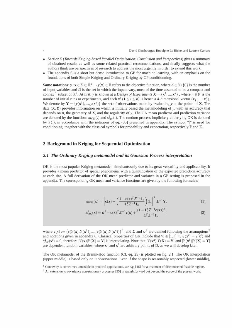
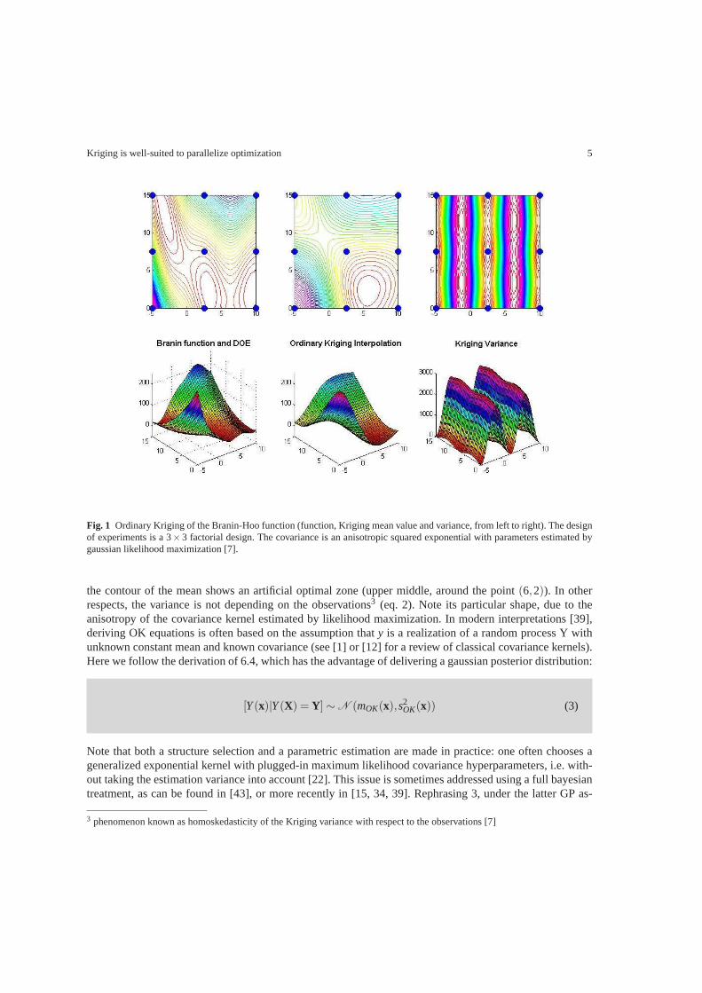
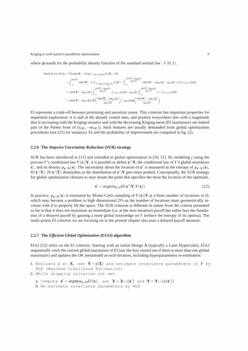
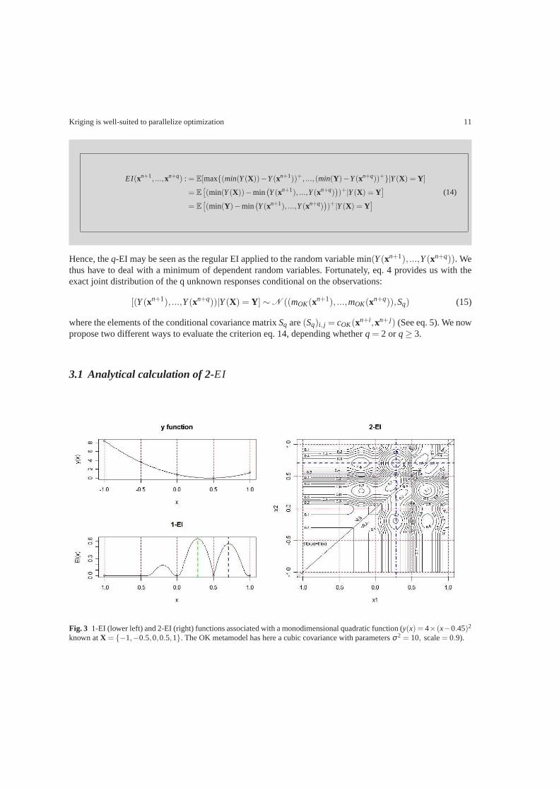
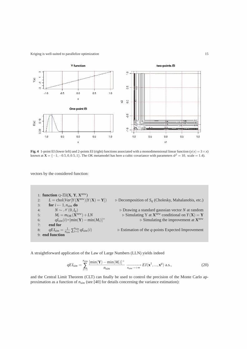
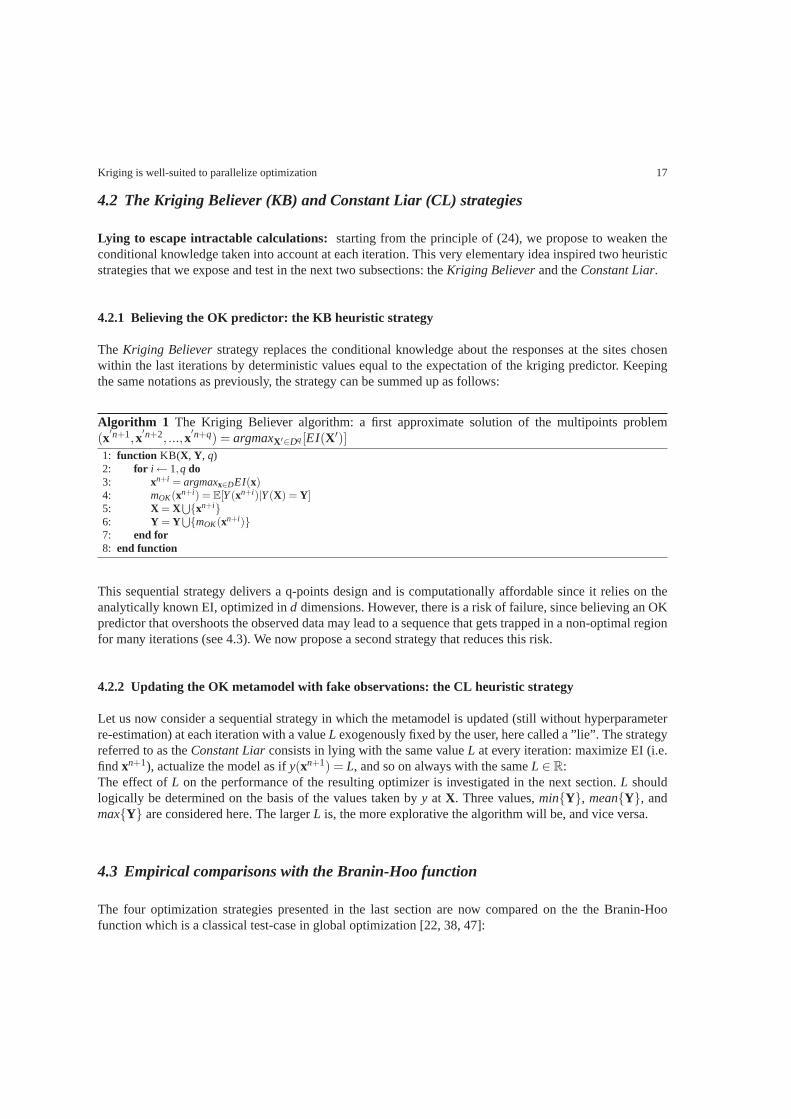
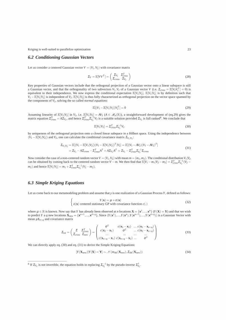
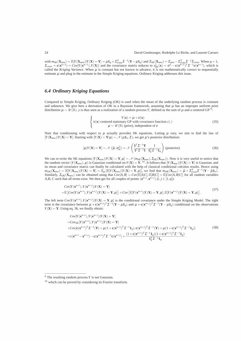mization problems for deterministic codes The simulator is seen as black-box functiony with d-dimensionalvector of inputs and scalar output the latter being often obtained as combination of several responsesMeta-models also calledsurrogate models are simplified representations ofy They can be used for predictingvalues ofy outside the initial design or visualizing the influence of each variable ony [27 43] They may alsoguide further sampling decisions for various purposes such as refining the exploration of the input space inpreferential zones or optimizing the functiony [22] Classical surrogates include radial basis functions[37]interpolation splines [52] neural nets [8] (deterministicmetamodels) or linear and non-linear regression[2] and Kriging [7] (probabilistic metamodels) We concentrate here on the advantages of probabilisticmetamodels for parallel exploration and optimization with a particular focus on the virtues of Kriging

12 Where Computational Intelligence and Kriging meet

Computational intelligence (CI) methods share in variousproportions four features

An history going from experiments to theory CI methods very often originate from empirical comput-ing experiments in particular from experiments that mimick natural processes (eg neural networks [4]ant colony optimization [5] simulated annealing [25]) Later on as researchers use and analyze themtheory develops and their mathematical content grows A good example is provided by the evolutionaryalgorithms [9] which have progressively mixed the genetic metaphor and stochastic optimization theory

An indirect problem representation In standard evolutionary optimization methods knowledgeaboutthe cost function takes the indirect form of a set of well-performing points known as ldquocurrent populationrdquoSuch set of points is an implicit partial representation of a function In fuzzy methods the probabilitydensity functions of the uncertain variables are averaged out Such indirect representations enable to workwith few mathematical assumptions and have broadened the range of applicability of CI methods

Parallelized decision process Most CI approaches are inherently parallel For example the evolution-ary or particle swarm optimization [24] methods process sets of points in parallel Neural networks havea internal parallel structure Today parallelism is crucial for taking advantage of the increasingly dis-tributed computing capacity The parallel decision makingpossibilities are related to the indirect problemrepresentations (through set of points distributions) and to the use of randomness in the decision process

Heuristics Implicit problem representations and the empirical genesis of the CI methods rarely allowmathematical proofs of the methods properties Most CI methods are thusheuristics

Kriging has recently gained popularity among several research communities related to CI ranging fromData Mining[16] andBayesian Statistics[34 48] toMachine Learning[39] where it is linked toGaussianProcess Regression[53] andKernel Method[12] Recent works [17 30 31] illustrate the practical relevanceof Kriging to approximate computer codes in application areas such as aerospace engineering or materialsscience Indeed probabilistic metamodels like Kriging seem to be particularly adapted for the optimizationof black-box functions as analyzed and illustrated in the excellent article [20] The current Chapter is de-voted to the optimization of black-box functions using a kriging metamodel [14 22 49 51] Let us nowstress some essential relationships between Kriging and CIby revisiting the above list of features

A history from field studies to mathematical statistics Kriging comes from the earth sciences [29 33]and has been progressively developed since the 1950rsquos alongwith the discipline calledgeostatistics[2332] Originally aimed at estimating natural ressources in mining applications it has later been adaptedto address very general interpolation and approximation problems [42 43] The word ldquokrigingrdquo comes
















1 xid)






mOK(x) =

[

c(x)+

(


1Tn Σminus11n

)

1n

]T

Σminus1Y (1)



1Tn Σminus11n

(2)

wherec(x) =(




















n Σminus11n

]

(5)















(7)





= E[


= Φ(

min(Y)minusmOK(x)

sOK(x)

)

(9)










min(Y)minusmOK(x)

sOK(x)

)

+sOK(x)φ(

min(Y)minusmOK(x)

sOK(x)

)

(11)




=int min(Y)



int






int




min(Y)minusmKO(x)

sKO(x)

)

+sKO(x)φ(

min(Y)minusmKO(x)

sKO(x)

)


















xn+q) = max(

I(xn+1) I(xn+q))

= max(


=(


(13)





= E[

(min(Y(X))minusmin(

Y(xn+1) Y(xn+q))

)+|Y(X) = Y]

= E[

(min(Y)minusmin(

Y(xn+1) Y(xn+q))

)+|Y(X) = Y]

(14)



















σ2i| j = σ2


i (1minusρ212)

(16)


Step 1





5 we get





Step 2











E[1Y2leY1|Y1] = Φ(

Y1minusm2|1s2|1

)

= Φ

Y1minusm2minus c12

σ21

(Y1minusm1)

σ2

radic

1minusρ212


E[


]

=

N11N1le

min(Y)minusm1σ1

Φ


σ2

radic

1minusρ212

= E[



σ1 β1 =

m1minusm2

σ2

radic

1minusρ212


σ2

radic

1minusρ212

(17)


int γ1


α1

2π

int γ1


2 du


(

radic


1+α21

)2

+β 2

11+α2


radic2πφ

(radic

β 21

1+α21

)

int γ1

minusinfine

minus

radic(1+α2

1 )u+α1β1radic

1+α21

2

2 du=

2πφ(radic

β 21

1+α21

)

radic

(1+α21)

int

radic(1+α2

1)γ1+α1β1radic

1+α21

minusinfin

eminusv2

2radic

2πdv





α1φ(radic

β 21

1+α21

)

radic

(1+α21)

Φ

radic

(1+α21)γ1 +

α1β1radic

1+α21


σ21 c12minusσ2

1c12minusσ2

1 σ22 +σ2

1 minus2c12

)




x2)+B(x2x1) (18)

where


ε(x1x2) = α1φ(

|β1|radic(1+α2

1)

)

Φ(

(1+α21)

12

(

γ + α1β11+α2

1

))


δ (x1x2) = CDF(Γ )

(

min(Y)minusm1

m1minusm2

)













nsimsumnsim



qEIsim =nsim

sumi=1



EI(x1 xq) as (20)



radicnsim

(


Var[I(x1 xq)]

)


N (01) in law (21)



(xprimen+1

xprimen+2









E[


(23)



int

uisinR j

[

E[


fY(X1 j )|Y(X)=Y(u)du (24)










⋃xn+i6 Y = Y











⋃xn+i5 Y = Y





(25)


prime1 = x1+5

15 andxprime2 = x2



1minusθ2h22 (26)


























6 Appendix






(27)





ΣV = E[VVT ] =

(

ΣV1 ΣTcross

Σcross ΣV2

)

(28)



E[(V1minusE[V1|V2])VT2 ] = 0 (29)





V2V2 (30)






V2Σcross

(31)


crossΣminus1V2


crossΣminus1V2

(V2minusm2)




(32)


Σtot =

(

Σ ΣTcross

Σcross Σnew

)

=



(33)















microσ2micro)

= N

(


1

1Tq Σminus11q

)

(posterior) (36)




=E[


+Cov[


(37)






1Tq Σminus11q

(38)



References





















680































Introduction















Appendix





References
















1 xid)






mOK(x) =

[

c(x)+

(


1Tn Σminus11n

)

1n

]T

Σminus1Y (1)



1Tn Σminus11n

(2)

wherec(x) =(




















n Σminus11n

]

(5)















(7)





= E[


= Φ(

min(Y)minusmOK(x)

sOK(x)

)

(9)










min(Y)minusmOK(x)

sOK(x)

)

+sOK(x)φ(

min(Y)minusmOK(x)

sOK(x)

)

(11)




=int min(Y)



int






int




min(Y)minusmKO(x)

sKO(x)

)

+sKO(x)φ(

min(Y)minusmKO(x)

sKO(x)

)


















xn+q) = max(

I(xn+1) I(xn+q))

= max(


=(


(13)





= E[

(min(Y(X))minusmin(

Y(xn+1) Y(xn+q))

)+|Y(X) = Y]

= E[

(min(Y)minusmin(

Y(xn+1) Y(xn+q))

)+|Y(X) = Y]

(14)



















σ2i| j = σ2


i (1minusρ212)

(16)


Step 1





5 we get





Step 2











E[1Y2leY1|Y1] = Φ(

Y1minusm2|1s2|1

)

= Φ

Y1minusm2minus c12

σ21

(Y1minusm1)

σ2

radic

1minusρ212


E[


]

=

N11N1le

min(Y)minusm1σ1

Φ


σ2

radic

1minusρ212

= E[



σ1 β1 =

m1minusm2

σ2

radic

1minusρ212


σ2

radic

1minusρ212

(17)


int γ1


α1

2π

int γ1


2 du


(

radic


1+α21

)2

+β 2

11+α2


radic2πφ

(radic

β 21

1+α21

)

int γ1

minusinfine

minus

radic(1+α2

1 )u+α1β1radic

1+α21

2

2 du=

2πφ(radic

β 21

1+α21

)

radic

(1+α21)

int

radic(1+α2

1)γ1+α1β1radic

1+α21

minusinfin

eminusv2

2radic

2πdv





α1φ(radic

β 21

1+α21

)

radic

(1+α21)

Φ

radic

(1+α21)γ1 +

α1β1radic

1+α21


σ21 c12minusσ2

1c12minusσ2

1 σ22 +σ2

1 minus2c12

)




x2)+B(x2x1) (18)

where


ε(x1x2) = α1φ(

|β1|radic(1+α2

1)

)

Φ(

(1+α21)

12

(

γ + α1β11+α2

1

))


δ (x1x2) = CDF(Γ )

(

min(Y)minusm1

m1minusm2

)













nsimsumnsim



qEIsim =nsim

sumi=1



EI(x1 xq) as (20)



radicnsim

(


Var[I(x1 xq)]

)


N (01) in law (21)



(xprimen+1

xprimen+2









E[


(23)



int

uisinR j

[

E[


fY(X1 j )|Y(X)=Y(u)du (24)










⋃xn+i6 Y = Y











⋃xn+i5 Y = Y





(25)


prime1 = x1+5

15 andxprime2 = x2



1minusθ2h22 (26)


























6 Appendix






(27)





ΣV = E[VVT ] =

(

ΣV1 ΣTcross

Σcross ΣV2

)

(28)



E[(V1minusE[V1|V2])VT2 ] = 0 (29)





V2V2 (30)






V2Σcross

(31)


crossΣminus1V2


crossΣminus1V2

(V2minusm2)




(32)


Σtot =

(

Σ ΣTcross

Σcross Σnew

)

=



(33)















microσ2micro)

= N

(


1

1Tq Σminus11q

)

(posterior) (36)




=E[


+Cov[


(37)






1Tq Σminus11q

(38)



References





















680































Introduction















Appendix





References














n Σminus11n

]

(5)















(7)





= E[


= Φ(

min(Y)minusmOK(x)

sOK(x)

)

(9)










min(Y)minusmOK(x)

sOK(x)

)

+sOK(x)φ(

min(Y)minusmOK(x)

sOK(x)

)

(11)




=int min(Y)



int






int




min(Y)minusmKO(x)

sKO(x)

)

+sKO(x)φ(

min(Y)minusmKO(x)

sKO(x)

)


















xn+q) = max(

I(xn+1) I(xn+q))

= max(


=(


(13)





= E[

(min(Y(X))minusmin(

Y(xn+1) Y(xn+q))

)+|Y(X) = Y]

= E[

(min(Y)minusmin(

Y(xn+1) Y(xn+q))

)+|Y(X) = Y]

(14)



















σ2i| j = σ2


i (1minusρ212)

(16)


Step 1





5 we get





Step 2











E[1Y2leY1|Y1] = Φ(

Y1minusm2|1s2|1

)

= Φ

Y1minusm2minus c12

σ21

(Y1minusm1)

σ2

radic

1minusρ212


E[


]

=

N11N1le

min(Y)minusm1σ1

Φ


σ2

radic

1minusρ212

= E[



σ1 β1 =

m1minusm2

σ2

radic

1minusρ212


σ2

radic

1minusρ212

(17)


int γ1


α1

2π

int γ1


2 du


(

radic


1+α21

)2

+β 2

11+α2


radic2πφ

(radic

β 21

1+α21

)

int γ1

minusinfine

minus

radic(1+α2

1 )u+α1β1radic

1+α21

2

2 du=

2πφ(radic

β 21

1+α21

)

radic

(1+α21)

int

radic(1+α2

1)γ1+α1β1radic

1+α21

minusinfin

eminusv2

2radic

2πdv





α1φ(radic

β 21

1+α21

)

radic

(1+α21)

Φ

radic

(1+α21)γ1 +

α1β1radic

1+α21


σ21 c12minusσ2

1c12minusσ2

1 σ22 +σ2

1 minus2c12

)




x2)+B(x2x1) (18)

where


ε(x1x2) = α1φ(

|β1|radic(1+α2

1)

)

Φ(

(1+α21)

12

(

γ + α1β11+α2

1

))


δ (x1x2) = CDF(Γ )

(

min(Y)minusm1

m1minusm2

)













nsimsumnsim



qEIsim =nsim

sumi=1



EI(x1 xq) as (20)



radicnsim

(


Var[I(x1 xq)]

)


N (01) in law (21)



(xprimen+1

xprimen+2









E[


(23)



int

uisinR j

[

E[


fY(X1 j )|Y(X)=Y(u)du (24)










⋃xn+i6 Y = Y











⋃xn+i5 Y = Y





(25)


prime1 = x1+5

15 andxprime2 = x2



1minusθ2h22 (26)


























6 Appendix






(27)





ΣV = E[VVT ] =

(

ΣV1 ΣTcross

Σcross ΣV2

)

(28)



E[(V1minusE[V1|V2])VT2 ] = 0 (29)





V2V2 (30)






V2Σcross

(31)


crossΣminus1V2


crossΣminus1V2

(V2minusm2)




(32)


Σtot =

(

Σ ΣTcross

Σcross Σnew

)

=



(33)















microσ2micro)

= N

(


1

1Tq Σminus11q

)

(posterior) (36)




=E[


+Cov[


(37)






1Tq Σminus11q

(38)



References





















680































Introduction















Appendix





References








(7)





= E[


= Φ(

min(Y)minusmOK(x)

sOK(x)

)

(9)










min(Y)minusmOK(x)

sOK(x)

)

+sOK(x)φ(

min(Y)minusmOK(x)

sOK(x)

)

(11)




=int min(Y)



int






int




min(Y)minusmKO(x)

sKO(x)

)

+sKO(x)φ(

min(Y)minusmKO(x)

sKO(x)

)


















xn+q) = max(

I(xn+1) I(xn+q))

= max(


=(


(13)





= E[

(min(Y(X))minusmin(

Y(xn+1) Y(xn+q))

)+|Y(X) = Y]

= E[

(min(Y)minusmin(

Y(xn+1) Y(xn+q))

)+|Y(X) = Y]

(14)



















σ2i| j = σ2


i (1minusρ212)

(16)


Step 1





5 we get





Step 2











E[1Y2leY1|Y1] = Φ(

Y1minusm2|1s2|1

)

= Φ

Y1minusm2minus c12

σ21

(Y1minusm1)

σ2

radic

1minusρ212


E[


]

=

N11N1le

min(Y)minusm1σ1

Φ


σ2

radic

1minusρ212

= E[



σ1 β1 =

m1minusm2

σ2

radic

1minusρ212


σ2

radic

1minusρ212

(17)


int γ1


α1

2π

int γ1


2 du


(

radic


1+α21

)2

+β 2

11+α2


radic2πφ

(radic

β 21

1+α21

)

int γ1

minusinfine

minus

radic(1+α2

1 )u+α1β1radic

1+α21

2

2 du=

2πφ(radic

β 21

1+α21

)

radic

(1+α21)

int

radic(1+α2

1)γ1+α1β1radic

1+α21

minusinfin

eminusv2

2radic

2πdv





α1φ(radic

β 21

1+α21

)

radic

(1+α21)

Φ

radic

(1+α21)γ1 +

α1β1radic

1+α21


σ21 c12minusσ2

1c12minusσ2

1 σ22 +σ2

1 minus2c12

)




x2)+B(x2x1) (18)

where


ε(x1x2) = α1φ(

|β1|radic(1+α2

1)

)

Φ(

(1+α21)

12

(

γ + α1β11+α2

1

))


δ (x1x2) = CDF(Γ )

(

min(Y)minusm1

m1minusm2

)













nsimsumnsim



qEIsim =nsim

sumi=1



EI(x1 xq) as (20)



radicnsim

(


Var[I(x1 xq)]

)


N (01) in law (21)



(xprimen+1

xprimen+2









E[


(23)



int

uisinR j

[

E[


fY(X1 j )|Y(X)=Y(u)du (24)










⋃xn+i6 Y = Y











⋃xn+i5 Y = Y





(25)


prime1 = x1+5

15 andxprime2 = x2



1minusθ2h22 (26)


























6 Appendix






(27)





ΣV = E[VVT ] =

(

ΣV1 ΣTcross

Σcross ΣV2

)

(28)



E[(V1minusE[V1|V2])VT2 ] = 0 (29)





V2V2 (30)






V2Σcross

(31)


crossΣminus1V2


crossΣminus1V2

(V2minusm2)




(32)


Σtot =

(

Σ ΣTcross

Σcross Σnew

)

=



(33)















microσ2micro)

= N

(


1

1Tq Σminus11q

)

(posterior) (36)




=E[


+Cov[


(37)






1Tq Σminus11q

(38)



References





















680































Introduction















Appendix





References








min(Y)minusmOK(x)

sOK(x)

)

+sOK(x)φ(

min(Y)minusmOK(x)

sOK(x)

)

(11)




=int min(Y)



int






int




min(Y)minusmKO(x)

sKO(x)

)

+sKO(x)φ(

min(Y)minusmKO(x)

sKO(x)

)


















xn+q) = max(

I(xn+1) I(xn+q))

= max(


=(


(13)





= E[

(min(Y(X))minusmin(

Y(xn+1) Y(xn+q))

)+|Y(X) = Y]

= E[

(min(Y)minusmin(

Y(xn+1) Y(xn+q))

)+|Y(X) = Y]

(14)



















σ2i| j = σ2


i (1minusρ212)

(16)


Step 1





5 we get





Step 2











E[1Y2leY1|Y1] = Φ(

Y1minusm2|1s2|1

)

= Φ

Y1minusm2minus c12

σ21

(Y1minusm1)

σ2

radic

1minusρ212


E[


]

=

N11N1le

min(Y)minusm1σ1

Φ


σ2

radic

1minusρ212

= E[



σ1 β1 =

m1minusm2

σ2

radic

1minusρ212


σ2

radic

1minusρ212

(17)


int γ1


α1

2π

int γ1


2 du


(

radic


1+α21

)2

+β 2

11+α2


radic2πφ

(radic

β 21

1+α21

)

int γ1

minusinfine

minus

radic(1+α2

1 )u+α1β1radic

1+α21

2

2 du=

2πφ(radic

β 21

1+α21

)

radic

(1+α21)

int

radic(1+α2

1)γ1+α1β1radic

1+α21

minusinfin

eminusv2

2radic

2πdv





α1φ(radic

β 21

1+α21

)

radic

(1+α21)

Φ

radic

(1+α21)γ1 +

α1β1radic

1+α21


σ21 c12minusσ2

1c12minusσ2

1 σ22 +σ2

1 minus2c12

)




x2)+B(x2x1) (18)

where


ε(x1x2) = α1φ(

|β1|radic(1+α2

1)

)

Φ(

(1+α21)

12

(

γ + α1β11+α2

1

))


δ (x1x2) = CDF(Γ )

(

min(Y)minusm1

m1minusm2

)













nsimsumnsim



qEIsim =nsim

sumi=1



EI(x1 xq) as (20)



radicnsim

(


Var[I(x1 xq)]

)


N (01) in law (21)



(xprimen+1

xprimen+2









E[


(23)



int

uisinR j

[

E[


fY(X1 j )|Y(X)=Y(u)du (24)










⋃xn+i6 Y = Y











⋃xn+i5 Y = Y





(25)


prime1 = x1+5

15 andxprime2 = x2



1minusθ2h22 (26)


























6 Appendix






(27)





ΣV = E[VVT ] =

(

ΣV1 ΣTcross

Σcross ΣV2

)

(28)



E[(V1minusE[V1|V2])VT2 ] = 0 (29)





V2V2 (30)






V2Σcross

(31)


crossΣminus1V2


crossΣminus1V2

(V2minusm2)




(32)


Σtot =

(

Σ ΣTcross

Σcross Σnew

)

=



(33)















microσ2micro)

= N

(


1

1Tq Σminus11q

)

(posterior) (36)




=E[


+Cov[


(37)






1Tq Σminus11q

(38)



References





















680































Introduction















Appendix





References




=int min(Y)



int






int




min(Y)minusmKO(x)

sKO(x)

)

+sKO(x)φ(

min(Y)minusmKO(x)

sKO(x)

)


















xn+q) = max(

I(xn+1) I(xn+q))

= max(


=(


(13)





= E[

(min(Y(X))minusmin(

Y(xn+1) Y(xn+q))

)+|Y(X) = Y]

= E[

(min(Y)minusmin(

Y(xn+1) Y(xn+q))

)+|Y(X) = Y]

(14)



















σ2i| j = σ2


i (1minusρ212)

(16)


Step 1





5 we get





Step 2











E[1Y2leY1|Y1] = Φ(

Y1minusm2|1s2|1

)

= Φ

Y1minusm2minus c12

σ21

(Y1minusm1)

σ2

radic

1minusρ212


E[


]

=

N11N1le

min(Y)minusm1σ1

Φ


σ2

radic

1minusρ212

= E[



σ1 β1 =

m1minusm2

σ2

radic

1minusρ212


σ2

radic

1minusρ212

(17)


int γ1


α1

2π

int γ1


2 du


(

radic


1+α21

)2

+β 2

11+α2


radic2πφ

(radic

β 21

1+α21

)

int γ1

minusinfine

minus

radic(1+α2

1 )u+α1β1radic

1+α21

2

2 du=

2πφ(radic

β 21

1+α21

)

radic

(1+α21)

int

radic(1+α2

1)γ1+α1β1radic

1+α21

minusinfin

eminusv2

2radic

2πdv





α1φ(radic

β 21

1+α21

)

radic

(1+α21)

Φ

radic

(1+α21)γ1 +

α1β1radic

1+α21


σ21 c12minusσ2

1c12minusσ2

1 σ22 +σ2

1 minus2c12

)




x2)+B(x2x1) (18)

where


ε(x1x2) = α1φ(

|β1|radic(1+α2

1)

)

Φ(

(1+α21)

12

(

γ + α1β11+α2

1

))


δ (x1x2) = CDF(Γ )

(

min(Y)minusm1

m1minusm2

)













nsimsumnsim



qEIsim =nsim

sumi=1



EI(x1 xq) as (20)



radicnsim

(


Var[I(x1 xq)]

)


N (01) in law (21)



(xprimen+1

xprimen+2









E[


(23)



int

uisinR j

[

E[


fY(X1 j )|Y(X)=Y(u)du (24)










⋃xn+i6 Y = Y











⋃xn+i5 Y = Y





(25)


prime1 = x1+5

15 andxprime2 = x2



1minusθ2h22 (26)


























6 Appendix






(27)





ΣV = E[VVT ] =

(

ΣV1 ΣTcross

Σcross ΣV2

)

(28)



E[(V1minusE[V1|V2])VT2 ] = 0 (29)





V2V2 (30)






V2Σcross

(31)


crossΣminus1V2


crossΣminus1V2

(V2minusm2)




(32)


Σtot =

(

Σ ΣTcross

Σcross Σnew

)

=



(33)















microσ2micro)

= N

(


1

1Tq Σminus11q

)

(posterior) (36)




=E[


+Cov[


(37)






1Tq Σminus11q

(38)



References





















680































Introduction















Appendix





References








xn+q) = max(

I(xn+1) I(xn+q))

= max(


=(


(13)





= E[

(min(Y(X))minusmin(

Y(xn+1) Y(xn+q))

)+|Y(X) = Y]

= E[

(min(Y)minusmin(

Y(xn+1) Y(xn+q))

)+|Y(X) = Y]

(14)



















σ2i| j = σ2


i (1minusρ212)

(16)


Step 1





5 we get





Step 2











E[1Y2leY1|Y1] = Φ(

Y1minusm2|1s2|1

)

= Φ

Y1minusm2minus c12

σ21

(Y1minusm1)

σ2

radic

1minusρ212


E[


]

=

N11N1le

min(Y)minusm1σ1

Φ


σ2

radic

1minusρ212

= E[



σ1 β1 =

m1minusm2

σ2

radic

1minusρ212


σ2

radic

1minusρ212

(17)


int γ1


α1

2π

int γ1


2 du


(

radic


1+α21

)2

+β 2

11+α2


radic2πφ

(radic

β 21

1+α21

)

int γ1

minusinfine

minus

radic(1+α2

1 )u+α1β1radic

1+α21

2

2 du=

2πφ(radic

β 21

1+α21

)

radic

(1+α21)

int

radic(1+α2

1)γ1+α1β1radic

1+α21

minusinfin

eminusv2

2radic

2πdv





α1φ(radic

β 21

1+α21

)

radic

(1+α21)

Φ

radic

(1+α21)γ1 +

α1β1radic

1+α21


σ21 c12minusσ2

1c12minusσ2

1 σ22 +σ2

1 minus2c12

)




x2)+B(x2x1) (18)

where


ε(x1x2) = α1φ(

|β1|radic(1+α2

1)

)

Φ(

(1+α21)

12

(

γ + α1β11+α2

1

))


δ (x1x2) = CDF(Γ )

(

min(Y)minusm1

m1minusm2

)













nsimsumnsim



qEIsim =nsim

sumi=1



EI(x1 xq) as (20)



radicnsim

(


Var[I(x1 xq)]

)


N (01) in law (21)



(xprimen+1

xprimen+2









E[


(23)



int

uisinR j

[

E[


fY(X1 j )|Y(X)=Y(u)du (24)










⋃xn+i6 Y = Y











⋃xn+i5 Y = Y





(25)


prime1 = x1+5

15 andxprime2 = x2



1minusθ2h22 (26)


























6 Appendix






(27)





ΣV = E[VVT ] =

(

ΣV1 ΣTcross

Σcross ΣV2

)

(28)



E[(V1minusE[V1|V2])VT2 ] = 0 (29)





V2V2 (30)






V2Σcross

(31)


crossΣminus1V2


crossΣminus1V2

(V2minusm2)




(32)


Σtot =

(

Σ ΣTcross

Σcross Σnew

)

=



(33)















microσ2micro)

= N

(


1

1Tq Σminus11q

)

(posterior) (36)




=E[


+Cov[


(37)






1Tq Σminus11q

(38)



References





















680































Introduction















Appendix





References



= E[

(min(Y(X))minusmin(

Y(xn+1) Y(xn+q))

)+|Y(X) = Y]

= E[

(min(Y)minusmin(

Y(xn+1) Y(xn+q))

)+|Y(X) = Y]

(14)



















σ2i| j = σ2


i (1minusρ212)

(16)


Step 1





5 we get





Step 2











E[1Y2leY1|Y1] = Φ(

Y1minusm2|1s2|1

)

= Φ

Y1minusm2minus c12

σ21

(Y1minusm1)

σ2

radic

1minusρ212


E[


]

=

N11N1le

min(Y)minusm1σ1

Φ


σ2

radic

1minusρ212

= E[



σ1 β1 =

m1minusm2

σ2

radic

1minusρ212


σ2

radic

1minusρ212

(17)


int γ1


α1

2π

int γ1


2 du


(

radic


1+α21

)2

+β 2

11+α2


radic2πφ

(radic

β 21

1+α21

)

int γ1

minusinfine

minus

radic(1+α2

1 )u+α1β1radic

1+α21

2

2 du=

2πφ(radic

β 21

1+α21

)

radic

(1+α21)

int

radic(1+α2

1)γ1+α1β1radic

1+α21

minusinfin

eminusv2

2radic

2πdv





α1φ(radic

β 21

1+α21

)

radic

(1+α21)

Φ

radic

(1+α21)γ1 +

α1β1radic

1+α21


σ21 c12minusσ2

1c12minusσ2

1 σ22 +σ2

1 minus2c12

)




x2)+B(x2x1) (18)

where


ε(x1x2) = α1φ(

|β1|radic(1+α2

1)

)

Φ(

(1+α21)

12

(

γ + α1β11+α2

1

))


δ (x1x2) = CDF(Γ )

(

min(Y)minusm1

m1minusm2

)













nsimsumnsim



qEIsim =nsim

sumi=1



EI(x1 xq) as (20)



radicnsim

(


Var[I(x1 xq)]

)


N (01) in law (21)



(xprimen+1

xprimen+2









E[


(23)



int

uisinR j

[

E[


fY(X1 j )|Y(X)=Y(u)du (24)










⋃xn+i6 Y = Y











⋃xn+i5 Y = Y





(25)


prime1 = x1+5

15 andxprime2 = x2



1minusθ2h22 (26)


























6 Appendix






(27)





ΣV = E[VVT ] =

(

ΣV1 ΣTcross

Σcross ΣV2

)

(28)



E[(V1minusE[V1|V2])VT2 ] = 0 (29)





V2V2 (30)






V2Σcross

(31)


crossΣminus1V2


crossΣminus1V2

(V2minusm2)




(32)


Σtot =

(

Σ ΣTcross

Σcross Σnew

)

=



(33)















microσ2micro)

= N

(


1

1Tq Σminus11q

)

(posterior) (36)




=E[


+Cov[


(37)






1Tq Σminus11q

(38)



References





















680































Introduction















Appendix





References













σ2i| j = σ2


i (1minusρ212)

(16)


Step 1





5 we get





Step 2











E[1Y2leY1|Y1] = Φ(

Y1minusm2|1s2|1

)

= Φ

Y1minusm2minus c12

σ21

(Y1minusm1)

σ2

radic

1minusρ212


E[


]

=

N11N1le

min(Y)minusm1σ1

Φ


σ2

radic

1minusρ212

= E[



σ1 β1 =

m1minusm2

σ2

radic

1minusρ212


σ2

radic

1minusρ212

(17)


int γ1


α1

2π

int γ1


2 du


(

radic


1+α21

)2

+β 2

11+α2


radic2πφ

(radic

β 21

1+α21

)

int γ1

minusinfine

minus

radic(1+α2

1 )u+α1β1radic

1+α21

2

2 du=

2πφ(radic

β 21

1+α21

)

radic

(1+α21)

int

radic(1+α2

1)γ1+α1β1radic

1+α21

minusinfin

eminusv2

2radic

2πdv





α1φ(radic

β 21

1+α21

)

radic

(1+α21)

Φ

radic

(1+α21)γ1 +

α1β1radic

1+α21


σ21 c12minusσ2

1c12minusσ2

1 σ22 +σ2

1 minus2c12

)




x2)+B(x2x1) (18)

where


ε(x1x2) = α1φ(

|β1|radic(1+α2

1)

)

Φ(

(1+α21)

12

(

γ + α1β11+α2

1

))


δ (x1x2) = CDF(Γ )

(

min(Y)minusm1

m1minusm2

)













nsimsumnsim



qEIsim =nsim

sumi=1



EI(x1 xq) as (20)



radicnsim

(


Var[I(x1 xq)]

)


N (01) in law (21)



(xprimen+1

xprimen+2









E[


(23)



int

uisinR j

[

E[


fY(X1 j )|Y(X)=Y(u)du (24)










⋃xn+i6 Y = Y











⋃xn+i5 Y = Y





(25)


prime1 = x1+5

15 andxprime2 = x2



1minusθ2h22 (26)


























6 Appendix






(27)





ΣV = E[VVT ] =

(

ΣV1 ΣTcross

Σcross ΣV2

)

(28)



E[(V1minusE[V1|V2])VT2 ] = 0 (29)





V2V2 (30)






V2Σcross

(31)


crossΣminus1V2


crossΣminus1V2

(V2minusm2)




(32)


Σtot =

(

Σ ΣTcross

Σcross Σnew

)

=



(33)















microσ2micro)

= N

(


1

1Tq Σminus11q

)

(posterior) (36)




=E[


+Cov[


(37)






1Tq Σminus11q

(38)



References





















680































Introduction















Appendix





References










E[1Y2leY1|Y1] = Φ(

Y1minusm2|1s2|1

)

= Φ

Y1minusm2minus c12

σ21

(Y1minusm1)

σ2

radic

1minusρ212


E[


]

=

N11N1le

min(Y)minusm1σ1

Φ


σ2

radic

1minusρ212

= E[



σ1 β1 =

m1minusm2

σ2

radic

1minusρ212


σ2

radic

1minusρ212

(17)


int γ1


α1

2π

int γ1


2 du


(

radic


1+α21

)2

+β 2

11+α2


radic2πφ

(radic

β 21

1+α21

)

int γ1

minusinfine

minus

radic(1+α2

1 )u+α1β1radic

1+α21

2

2 du=

2πφ(radic

β 21

1+α21

)

radic

(1+α21)

int

radic(1+α2

1)γ1+α1β1radic

1+α21

minusinfin

eminusv2

2radic

2πdv





α1φ(radic

β 21

1+α21

)

radic

(1+α21)

Φ

radic

(1+α21)γ1 +

α1β1radic

1+α21


σ21 c12minusσ2

1c12minusσ2

1 σ22 +σ2

1 minus2c12

)




x2)+B(x2x1) (18)

where


ε(x1x2) = α1φ(

|β1|radic(1+α2

1)

)

Φ(

(1+α21)

12

(

γ + α1β11+α2

1

))


δ (x1x2) = CDF(Γ )

(

min(Y)minusm1

m1minusm2

)













nsimsumnsim



qEIsim =nsim

sumi=1



EI(x1 xq) as (20)



radicnsim

(


Var[I(x1 xq)]

)


N (01) in law (21)



(xprimen+1

xprimen+2









E[


(23)



int

uisinR j

[

E[


fY(X1 j )|Y(X)=Y(u)du (24)










⋃xn+i6 Y = Y











⋃xn+i5 Y = Y





(25)


prime1 = x1+5

15 andxprime2 = x2



1minusθ2h22 (26)


























6 Appendix






(27)





ΣV = E[VVT ] =

(

ΣV1 ΣTcross

Σcross ΣV2

)

(28)



E[(V1minusE[V1|V2])VT2 ] = 0 (29)





V2V2 (30)






V2Σcross

(31)


crossΣminus1V2


crossΣminus1V2

(V2minusm2)




(32)


Σtot =

(

Σ ΣTcross

Σcross Σnew

)

=



(33)















microσ2micro)

= N

(


1

1Tq Σminus11q

)

(posterior) (36)




=E[


+Cov[


(37)






1Tq Σminus11q

(38)



References





















680































Introduction















Appendix





References



α1φ(radic

β 21

1+α21

)

radic

(1+α21)

Φ

radic

(1+α21)γ1 +

α1β1radic

1+α21


σ21 c12minusσ2

1c12minusσ2

1 σ22 +σ2

1 minus2c12

)




x2)+B(x2x1) (18)

where


ε(x1x2) = α1φ(

|β1|radic(1+α2

1)

)

Φ(

(1+α21)

12

(

γ + α1β11+α2

1

))


δ (x1x2) = CDF(Γ )

(

min(Y)minusm1

m1minusm2

)













nsimsumnsim



qEIsim =nsim

sumi=1



EI(x1 xq) as (20)



radicnsim

(


Var[I(x1 xq)]

)


N (01) in law (21)



(xprimen+1

xprimen+2









E[


(23)



int

uisinR j

[

E[


fY(X1 j )|Y(X)=Y(u)du (24)










⋃xn+i6 Y = Y











⋃xn+i5 Y = Y





(25)


prime1 = x1+5

15 andxprime2 = x2



1minusθ2h22 (26)


























6 Appendix






(27)





ΣV = E[VVT ] =

(

ΣV1 ΣTcross

Σcross ΣV2

)

(28)



E[(V1minusE[V1|V2])VT2 ] = 0 (29)





V2V2 (30)






V2Σcross

(31)


crossΣminus1V2


crossΣminus1V2

(V2minusm2)




(32)


Σtot =

(

Σ ΣTcross

Σcross Σnew

)

=



(33)















microσ2micro)

= N

(


1

1Tq Σminus11q

)

(posterior) (36)




=E[


+Cov[


(37)






1Tq Σminus11q

(38)



References





















680































Introduction















Appendix





References







nsimsumnsim



qEIsim =nsim

sumi=1



EI(x1 xq) as (20)



radicnsim

(


Var[I(x1 xq)]

)


N (01) in law (21)



(xprimen+1

xprimen+2









E[


(23)



int

uisinR j

[

E[


fY(X1 j )|Y(X)=Y(u)du (24)










⋃xn+i6 Y = Y











⋃xn+i5 Y = Y





(25)


prime1 = x1+5

15 andxprime2 = x2



1minusθ2h22 (26)


























6 Appendix






(27)





ΣV = E[VVT ] =

(

ΣV1 ΣTcross

Σcross ΣV2

)

(28)



E[(V1minusE[V1|V2])VT2 ] = 0 (29)





V2V2 (30)






V2Σcross

(31)


crossΣminus1V2


crossΣminus1V2

(V2minusm2)




(32)


Σtot =

(

Σ ΣTcross

Σcross Σnew

)

=



(33)















microσ2micro)

= N

(


1

1Tq Σminus11q

)

(posterior) (36)




=E[


+Cov[


(37)






1Tq Σminus11q

(38)



References





















680































Introduction















Appendix





References


radicnsim

(


Var[I(x1 xq)]

)


N (01) in law (21)



(xprimen+1

xprimen+2









E[


(23)



int

uisinR j

[

E[


fY(X1 j )|Y(X)=Y(u)du (24)










⋃xn+i6 Y = Y











⋃xn+i5 Y = Y





(25)


prime1 = x1+5

15 andxprime2 = x2



1minusθ2h22 (26)


























6 Appendix






(27)





ΣV = E[VVT ] =

(

ΣV1 ΣTcross

Σcross ΣV2

)

(28)



E[(V1minusE[V1|V2])VT2 ] = 0 (29)





V2V2 (30)






V2Σcross

(31)


crossΣminus1V2


crossΣminus1V2

(V2minusm2)




(32)


Σtot =

(

Σ ΣTcross

Σcross Σnew

)

=



(33)















microσ2micro)

= N

(


1

1Tq Σminus11q

)

(posterior) (36)




=E[


+Cov[


(37)






1Tq Σminus11q

(38)



References





















680































Introduction















Appendix





References









⋃xn+i6 Y = Y











⋃xn+i5 Y = Y





(25)


prime1 = x1+5

15 andxprime2 = x2



1minusθ2h22 (26)


























6 Appendix






(27)





ΣV = E[VVT ] =

(

ΣV1 ΣTcross

Σcross ΣV2

)

(28)



E[(V1minusE[V1|V2])VT2 ] = 0 (29)





V2V2 (30)






V2Σcross

(31)


crossΣminus1V2


crossΣminus1V2

(V2minusm2)




(32)


Σtot =

(

Σ ΣTcross

Σcross Σnew

)

=



(33)















microσ2micro)

= N

(


1

1Tq Σminus11q

)

(posterior) (36)




=E[


+Cov[


(37)






1Tq Σminus11q

(38)



References





















680































Introduction















Appendix





References





⋃xn+i5 Y = Y





(25)


prime1 = x1+5

15 andxprime2 = x2



1minusθ2h22 (26)


























6 Appendix






(27)





ΣV = E[VVT ] =

(

ΣV1 ΣTcross

Σcross ΣV2

)

(28)



E[(V1minusE[V1|V2])VT2 ] = 0 (29)





V2V2 (30)






V2Σcross

(31)


crossΣminus1V2


crossΣminus1V2

(V2minusm2)




(32)


Σtot =

(

Σ ΣTcross

Σcross Σnew

)

=



(33)















microσ2micro)

= N

(


1

1Tq Σminus11q

)

(posterior) (36)




=E[


+Cov[


(37)






1Tq Σminus11q

(38)



References





















680































Introduction















Appendix





References
























6 Appendix






(27)





ΣV = E[VVT ] =

(

ΣV1 ΣTcross

Σcross ΣV2

)

(28)



E[(V1minusE[V1|V2])VT2 ] = 0 (29)





V2V2 (30)






V2Σcross

(31)


crossΣminus1V2


crossΣminus1V2

(V2minusm2)




(32)


Σtot =

(

Σ ΣTcross

Σcross Σnew

)

=



(33)















microσ2micro)

= N

(


1

1Tq Σminus11q

)

(posterior) (36)




=E[


+Cov[


(37)






1Tq Σminus11q

(38)



References





















680































Introduction















Appendix





References




ΣV = E[VVT ] =

(

ΣV1 ΣTcross

Σcross ΣV2

)

(28)



E[(V1minusE[V1|V2])VT2 ] = 0 (29)





V2V2 (30)






V2Σcross

(31)


crossΣminus1V2


crossΣminus1V2

(V2minusm2)




(32)


Σtot =

(

Σ ΣTcross

Σcross Σnew

)

=



(33)















microσ2micro)

= N

(


1

1Tq Σminus11q

)

(posterior) (36)




=E[


+Cov[


(37)






1Tq Σminus11q

(38)



References





















680































Introduction















Appendix





References











microσ2micro)

= N

(


1

1Tq Σminus11q

)

(posterior) (36)




=E[


+Cov[


(37)






1Tq Σminus11q

(38)



References





















680































Introduction















Appendix





References


References





















680































Introduction















Appendix





References































Introduction















Appendix





References

kriging is well-suited to parallelize optimizationkriging is well-suited to parallelize optimization...

Documents