kung slides - cs.ioc.ee

Machine Learning for Compressive Privacy

S.Y. Kung

Princeton University

Professor S.Y. Kung

• Email: [email protected]

References:

• `Kernel Method and Machine Learning”, S.Y. Kung

Cambridge University Press (CUP), 2014.

• SPS Magazine: Invited Column on Compressive Privacy

Supplementary Materials:

• Tentative Power Point Slides (notes provided)

• DCA Paper (paper provided)


i. Overview of Big Data Analysis ii. Subspace and Visualization of Big Data (DCA) iii. Compressive Privacy in Brandeis Program iv. Differential Utility/Cost Advantage (DUCA) v. Nonlinear and Kernel Learning Machines


In the internet era, we experience a phenomenon of “digital everything”. Due to its quantitative (volume and velocity) and qualitative (variety) challenges, it is imperative to address various computational aspects of big data. For big data, the curse of high feature dimensionality is causing grave concerns on computational complexity and over-training.


i. Overview of Big Data Analysis

Old Moore’s Law will soon lose ground to New Moore’s Law on Massive Data Readily Captured in Digital format.

•VLSI gates Doubles every 1.5 years

•Data in digital format

Doubles every 2 years

Device Moore’s Law

The rise of Data Scientists [Schonberger12].

Data Moore’s Law

9

Quantitatively:

over 200 million emails are sent, 100 hours of video uploaded on Youtube every minute!!

Facebook: In 2012, Facebook had over one billion users and, more importantly, with over 100 billion social links…. Every day, more than 250 Million new photos added to Facebook.

Examples of Big Data

big= extremely high feature dimensionality:

• computational complexity • data over-training causing

performance downgrades.

Volume/Velocity: Curse of Dimensionality in Big Data

𝑴 ≫ 𝑵

𝑴

𝑵 ≫ 𝑴

big= extremely large-scale data size:

• computational complexity causing costly hardware, long computing time, and high processing power.

𝑵

11

“The era of trillions of sensors is upon us...."

3 Distributions of Learned Threshold: From Small to Large N

(N=Sample Number per Class)

accurate threshold =0

Error function

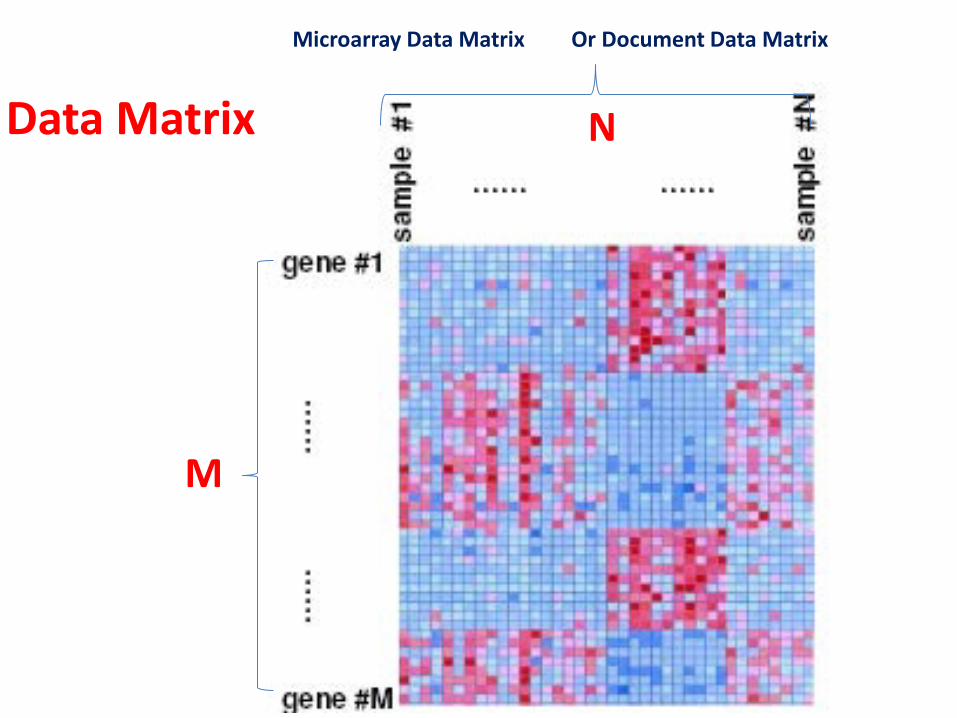
Data Matrix

M

N

Microarray Data Matrix Or Document Data Matrix

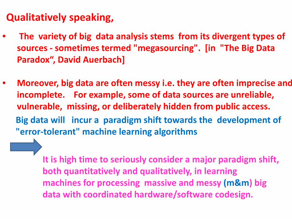
Qualitatively speaking,

Big data will incur a paradigm shift towards the development of "error-tolerant" machine learning algorithms

• The variety of big data analysis stems from its divergent types of

sources - sometimes termed "megasourcing". [in "The Big Data Paradox“, David Auerbach]

• Moreover, big data are often messy i.e. they are often imprecise and incomplete. For example, some of data sources are unreliable, vulnerable, missing, or deliberately hidden from public access.

It is high time to seriously consider a major paradigm shift, both quantitatively and qualitatively, in learning machines for processing massive and messy (m&m) big data with coordinated hardware/software codesign.

Big Data Variety: vectorial or non-vectorial data

Big Data Veracity: uncertain or imprecise data

An implicit principle behind big data analysis is

to make use of ALL of the available data,

vectorial or non-vectorial (i.e. the variety),

whether they are messy, imprecise, or

incomplete (i.e. the veracity).

Qualitatively:

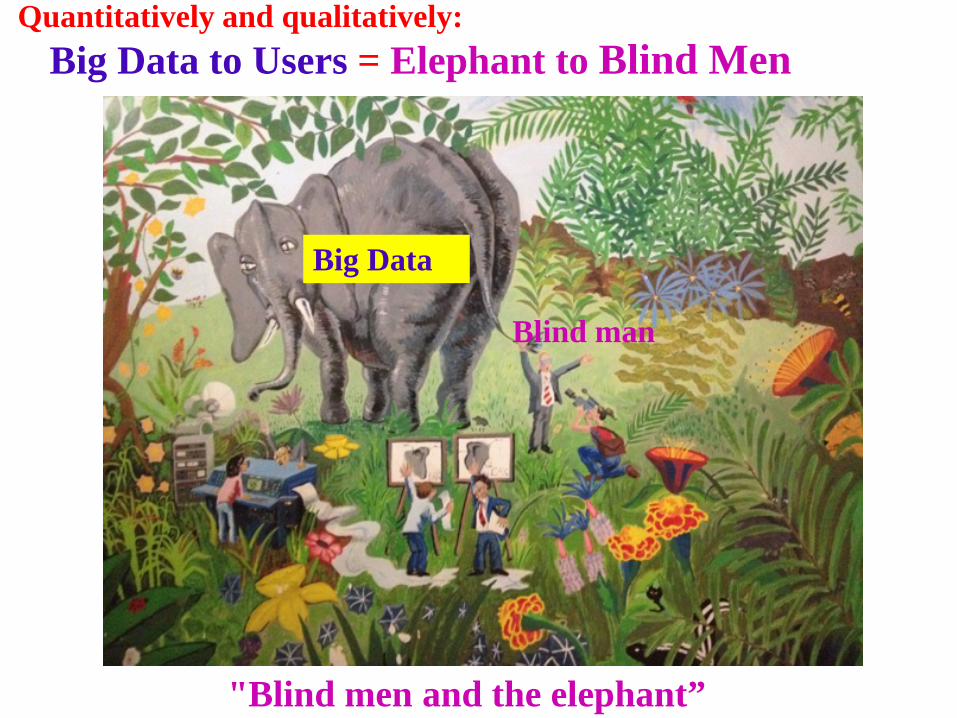
"Blind men and the elephant”

Big Data to Users = Elephant to Blind Men

Big Data

Blind man

Quantitatively and qualitatively:

Google Flu Trends detects a significant increase in H1N1 flu activity two-weeks earlier than CDC - using big data learning and cloud computing. A lot of hard work behind the success:

Google Flu Trends CDC

Jan 28, 2008

2007-2008 U.S. Flu Activity (Mid-Altlantic Region) pe

rcen

tage

• 45 keywords are chosen from 5M keywords • Half a Billion of mathematical models tried.

Objective of Machine Learning

The main function of machine learning is to convert the wealth of training data into useful knowledge by learning. data ≠ knowledge

Machine Learning is a research field study theories and technologies to adapt a system model based on training dataset, so that the learned model will be able to generalize and provide a correct classification or useful guidance even when inputs to the system are previously unknown.

Machine Learning System

Feature Engineering

Labeling Engineering

Much of the success of machine learning lies in an effective representation of the objects. Learning models such as deep learning and kernel machines can derive a much expanded vector space, from massive and messy big data, which may then be further extracted for classification. Such a learning methodology has had numerous successful and practical applications.

Feture Representation The secret of success of a machine learning system lies in finding an effective representation for the objects of interest. In a basic representation, an object is represented as a feature vector in a finite-dimensional vector space. Two common strategies: • dimension reduction: to battle over-training • dimension expansion: to battle under-training

x ⇒ z

x ⇒ φ


We shall explore various projection methods, e.g. PCA, for dimension reduction – a prelude to visualization and privacy preserving of big data. An important development is Discriminant Component Analysis (DCA), which offers a compression scheme to enhance privacy protection in contextual and collaborative learning environment.

An implicit principle behind big data analysis is to make use of ALL of the available data, vectorial or non-vectorial (i.e. the variety), whether they are messy, imprecise, or incomplete (i.e. the veracity). Massive digital data are being rapidly captured in digital format, including digital book/voice/image/video/commerce. They come from divergent types of sources, from physical (sensor/IoT) to social and cyber (web) types. Note that visualization tools are meant to supplement (instead of replace) the domain expertise (e.g. a cardiologist) and provide a big picture to help users formulate critical questions and subsequently postulate heuristic and insightful answers.

ii. Subspace and Visualization of Big Data (DCA)

Important Research Areas on Big Data By CCF vote, 55% goes to Visualization

Visualization

HPC System Integration

Revolutionary Algorithms

55%

Visualization of (High-Dimensional) Big Data

• It facilitates formulation of insightful questions and postulation of heuristic answers.

A picture is worth a thousand words!!

• Visualization offers an informal presentation of massive and messy big data and supplements (instead of replaces) the domain expertise (e.g. a cardiologist).

PCA/DCA serves as a good example/evidence!

Visualization

Multi-Dimensional scaling (MDS)

Deep Learning Auto-Encoder. Tree Clustering

Unsupervised • PCA (vector data) • KPCA(nonvector data)

Supervised • DCA (vector data) • KDCA(nonvector data)

K-means/ Kernel K-means

SOM/Kernel SOM Vectorization

Dimension Reduction

Visualization of (High-Dimensional) Big Data

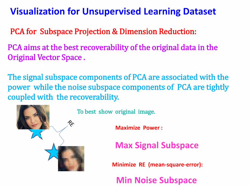
PCA for Subspace Projection & Dimension Reduction:

PCA aims at the best recoverability of the original data in the Original Vector Space . The signal subspace components of PCA are associated with the power while the noise subspace components of PCA are tightly coupled with the recoverability.

Min Noise Subspace

To best show original image.

Max Signal Subspace

Minimize RE (mean-square-error):

Maximize Power :

Visualization for Unsupervised Learning Dataset

[ ]

==

2

12111 x

xvvWxy

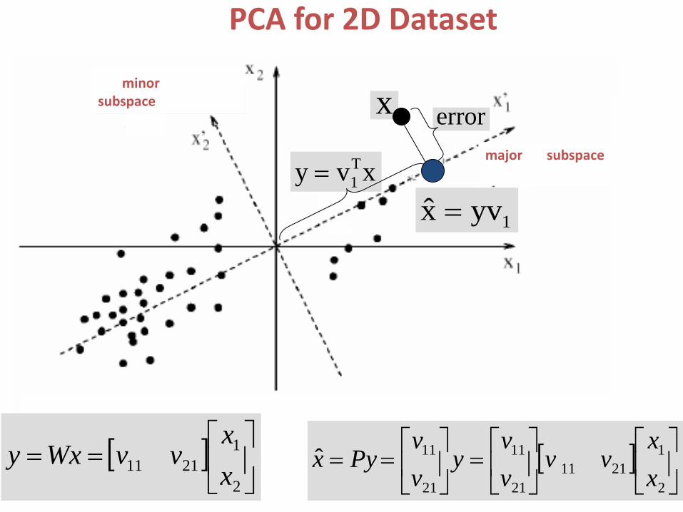
PCA for 2D Dataset

[ ]

=

==

2

12111

21

11

21

11ˆxx

vvvv

yvv

Pyx

xvy T1=

x errorsubspaceminor

1yvx̂ =

major subspace

minor subspace

The original input vector can be reconstructed from y as:

Trace Norm Criterion: M-Dimensional Case

Useful for Proof:

PCA in Trace-Norm Formulation:

[ ]

( )]WS[W argmax

ww

wSwargmaxW

T

IW W:RW

m

1i iTi

iTi

:WPCA

TmMtrace

=∈

=⊥

×=

≡ ∑

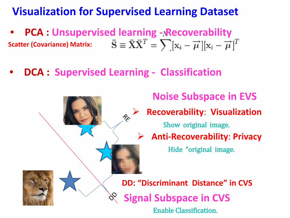
Visualization for Supervised Learning Dataset

Signal Subspace in CVS Enable Classification.

DD: “Discriminant Distance” in CVS

• PCA : Unsupervised learning - Recoverability Scatter (Covariance) Matrix:

( ) ∑∑==

==M

i

M

itrace

1i

1i

T p US U λ

This image cannot currently be displayed.


Minimize RE (mean-square-error):

Maximize Power :

• DCA : Supervised Learning - Classification

Recoverability: Visualization Noise Subspace in EVS

Show original image.

Anti-Recoverability: Privacy Hide “original image.

Signal Matrix = SB = Between-Class Matrix

Noise Matrix = SW = Within-Class Matrix

detrimental

For supervised (i.e. labeled) dataset with L classes:

WS S

WB SSS += = Signal Matrix + Noise Matrix

beneficiary SBS

∆

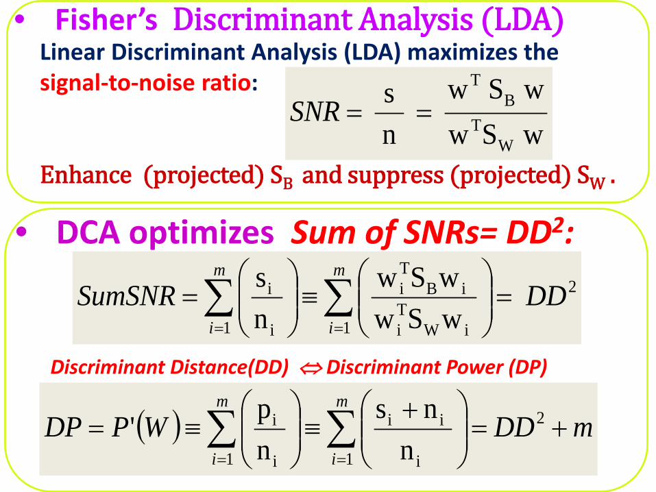
Linear Discriminant Analysis (LDA) maximizes the signal-to-noise ratio:

• Fisher’s Discriminant Analysis (LDA)

wSw wS w

n s

WT

BT

==SNR

• DCA optimizes Sum of SNRs= DD2: 2

1 iWTi

iBTi

1 i

i wSwwSw

ns DDSumSNR

m

i

m

i=

≡

= ∑∑

==

( ) mDDWPDPm

i

m

i+=

+≡

≡= ∑∑

==

2

1 i

ii

1 i

i n

nsnp'

Discriminant Distance(DD) ⇔ Discriminant Power (DP)

Enhance (projected) SB and suppress (projected) SW .

component analysis

Canonical Vector Space (CVS) Rotational Invariance of DD/DP

Mahalanobis Orthonormality = Canonical Orthonormality

IWSW WT = Rotational Invariant

Euclidean Orthonormality in the original EVS

IWWT = Not Rotational Invariant

DCA Optimization Criterion: Discriminant Power (DP)

⇒ Orthonormal Bases

Invariance of Orthonormality Invariance of DP (Redundancy)

⇒ Rotational Invariance (Visualization )

DD2 = Sum of SNRs

L-1

DD in CVS:

2

1iB

Ti

1 iWTi

iBTi w~S~w~

w~S~w~w~S~w~ DDSumSNR

m

i

m

i∑∑

==

==

=

Class-ceiling property

10:1 in compression ratio

where

( )

( ) ( ) ( ) W~~W~S~W~ w~S~w~

w~ I w~w~S~w~

wSwwSw'

T

1i

Ti

1w~w~

1 iTi

iTi

1 iWTi

iTi

iTi

Ptrace

WP

m

i

m

i

m

i

===

=

=

∑

∑∑

==

==

DP in CVS = Power in CVS

DCA ⇒

⇒ PCA

DCA and PCA are equivalent in CVS!

Preservation of DP under Coordinate Transformation

≡

Algebraically,

∑∑==

=

≡

m

i

m

iDP

1 iWTi

iTi

1 i

i

wSwwSw

np

whitening

PCA in whitened space

⌂’

L= 3, L-1=2

original space

canonical space

Data Laundry ⇒Canonical Vector Space (CVS) The canonical vector space is defined as the whitened space.

CVS EVS

Pictorially,

x = (Sw) - ½ x ~

re-Mapping

w = [Sw] -½T w ~

Forward Mapping:

DCA = PCA in CVS

PCA

Find the first m principal eigenvectors under the ``canonically normality" constraint that

Discriminant Matrix

Direct EVS Method: Trace Norm Optimizer

Backward Mapping:

i=1,2,…,m.

Principal Eigenvalues for the Signal Subspace:

Roles of DCA Eigenvalues DCA maximizes RDP and optimizes (minimizes/maximizes) RE for recoverability or anti-recoverability.

• Dimension Reduction (Cost, Power, Storage, Communication)

• Prediction Performance (Classification Accuracy in Prediction Phase)

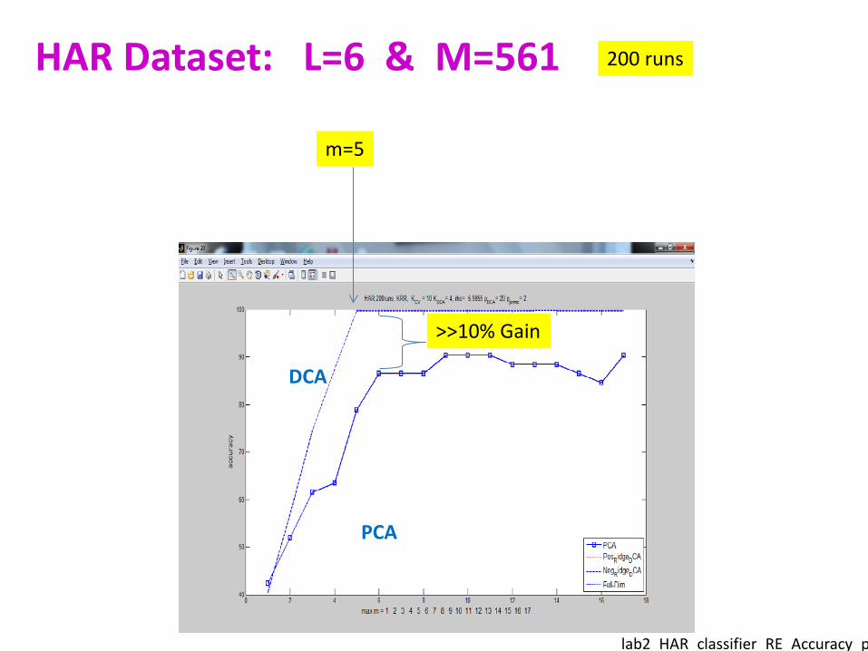
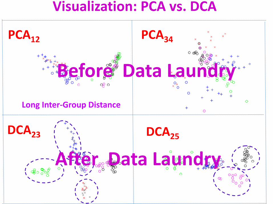
Simulation Results With the data laundry process, DCA (i.e. supervised-PCA) far outperforms PCA.

Visu

aliz

atio

n: D

CA v

s. P

CA

PCA PCA

DCA

m=5

200 runs HAR Dataset: L=6 & M=561

lab2 HAR classifier RE Accuracy p

>>10% Gain

DCA23

PCA12

DCA25

PCA34

Visualization: PCA vs. DCA

Long Inter-Group Distance

Before Data Laundry

After Data Laundry

In the internet era, we benefit greatly from the combination of packet switching, bandwidth, processing and storage capacities in the cloud. However, “big-data” often has a connotation of “big-brother”, since the data being collected on consumers like us is growing exponentially, attacks on our privacy are becoming a real threat. New technologies are needed to better assure our privacy protection when we upload personal data to the cloud. An important development is Discriminant Component Analysis (DCA), which offers a compression scheme to enhance privacy protection in contextual and collaborative learning environment. DCA can be viewed as a supervised PCA which can simultaneously rank order the (1) the sensitive components and (2) the desensitized components.


iii. Compressive Privacy in Brandeis Program

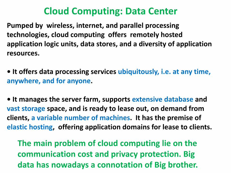
Pumped by wireless, internet, and parallel processing technologies, cloud computing offers remotely hosted application logic units, data stores, and a diversity of application resources. • It offers data processing services ubiquitously, i.e. at any time, anywhere, and for anyone. • It manages the server farm, supports extensive database and vast storage space, and is ready to lease out, on demand from clients, a variable number of machines. It has the premise of elastic hosting, offering application domains for lease to clients.

Cloud Computing: Data Center

The main problem of cloud computing lie on the communication cost and privacy protection. Big data has nowadays a connotation of Big brother.

Colorful water pipes cool one of Google’s data centers. The company sells user data to advertisers for targeted marketing campaigns. Connie Zhou/Google

Google’s Data Centers

With rapidly growing internet commerce, much of our daily activities are moving online, abundance of personal information (such as sale transactions) are being collected, stored, and circulated around the internet and cloud servers, often without the owner's knowledge

Machine learning Approach to Compressive Privacy

This raises an imminent concern on the protection and safety of sensitive and private data, i.e. ``Online Privacy", also known as ``Internet Privacy" or ``Cloud Privacy". This course presents some machine learning methods useful for and internet privacy preserving data mining, which has recently received a great deal of attention in the IT community.

When the control of data protection is left entirely to the cloud server, the data privacy will unfortunately become vulnerable to hacker attack or unauthorized leakage. It is therefore much safer to keep the control for data protection solely at the hand of the data owner and not taking chance with the cloud.

Why DARPA Brandeis Program?

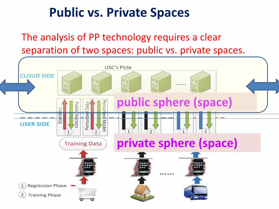
public sphere (space)

private sphere (space)

Public vs. Private Spaces

The analysis of PP technology requires a clear separation of two spaces: public vs. private spaces.

• Encrypted Data

• Decrypted Data

Public Space (Cloud)

Private Space (Client)

Encryption for Privacy Protection

• trusted authority

• data owners

• cloud server

Theme of the Brandeis Program: Control for data protection should be returned to the data owner rather than at leaving it at the mercy of the cloud server.

Why not Encryption? To ensure protection via encryption, during the processing in the ``public sphere", the input data of each owner and any intermediate results will only be revealed/decrypted to the trusted authority.

Nevertheless, there exists substantial chance of encountering hacker attack or unauthorized leakage, when leaving the data protection entirely to the hand/mercy of the cloud server.

Data owner should have control over data From the data privacy's perspective, the accessibility of data is divided into two separate spheres: (1) private sphere: where data owners generate and process decrypted data; and (2) public sphere: where cloud servers can generally access only encrypted data, with the exception that only the trusted authority may access decrypted data confidentially. When the control of data protection is left entirely to the cloud server, however, the data become vulnerable to hacker attack or unauthorized leakage. It is safer to let data owner control the data privacy and not to take chance with the cloud servers.

To this end, we must design privacy preserving information systems so that the shared/pushed data are only useful for the intended utility and not easily diverted for malicious privacy intrusion.

Build information systems so that the shared data could be • effective and relevant for the intended

utility (e.g. classification) • but not easily diverted to other

purposes (e.g. privacy).

DARPA Brandeis Program on Internet Privacy(IP)：

US$60M/4.5 Yrs.

Brandeis Mobile CRT

Raytheon BBN, Invincea

TA3: Human Data Interaction

TA1: Privacy Technologies

CMU, Tel Aviv U

TA4: Measuring Privacy

Cybernetica, U of Tartu

UC Berkeley, MIT, Cornel,

U MD

Iowa State U, Princeton

Stealth Software Technologies

TA3: Experimental

Prototype Systems

In emergency such as bomb threat, many mobile images from various sources may be voluntarily pushed to the command center for wide-scale forensic analysis. In this case, CP may be used to compute the dimension-reduced feature subspace which can (1) effectively identify the suspect(s) and (2) adequately obfuscate the face images of the innocent.

Mobile Information Flow

56

Control Center makes request for images near an incident.

User’s phone responds with some incident-relevant images per their privacy policy

User Application

Privacy Policy

PE Android Example: location = utility; face = privacy

More on Mobile PP Applications ”The Android platform provides several sensors that let you monitor the motion of a device. Two of these sensors are always hardware-based (the accelerometer and gyroscope)”, (Most devices have both gyroscope and accelerometer.) and ”three of these sensors can be either hardware-based or software-based (the gravity, linear acceleration, and rotation vector sensors).” Adapted from CC Liu, et al.

= private

DP ⇒

Adapted from CC Liu, et al D (data) = Activity (B/L) Location (W/L) Tabs (B/L) app (M)= speech , motion, ID, password

More on Mobile PP Applications

We need to develop new methods to jointly optimize two design considerations P & U: Privacy Protection & Utility Maximization .

Machine learning Approach to Privacy

Protection of Internet/Cloud Data

Objective: Explore information systems simultaneously perform

Utility Space Maximization: deliver intended data mining, classification, and learning tasks.

Privacy Space Minimization: safeguard personal/private information.

CP involves joint optimization over three design spaces: (i) Feature Space (ii) Utility Subspace; and (iii) Cost Subspace (i.e. Privacy Subspace).

Compression (PCA) Random Noise Random Transform

USC’s Pickle: A collaborative learning model built for MFCC speaker recognition - widely used in acoustic mobile applications - to enable speaker recognition without revealing the speech content itself.

public data

private data

Collaborative Learning for PP

• Single-user vs. Multi-user environments

• Centralized vs. Distributed Processing

• Unsupervised vs. Unsupervised Learning

Collaborative Learning for PP

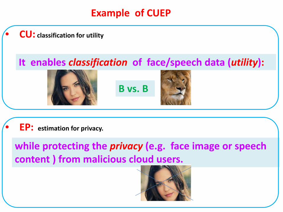
B vs. B

It enables classification of face/speech data (utility):

Example of CUEP

• CU: classification for utility

• EP: estimation for privacy.

while protecting the privacy (e.g. face image or speech content ) from malicious cloud users.

Original

Masked Data

Classification Personality Privacy

• CUEP Example classification formulation for utility but estimation for privacy.

“ i ll i f l i b i d j b d i l l d i lik SIFT

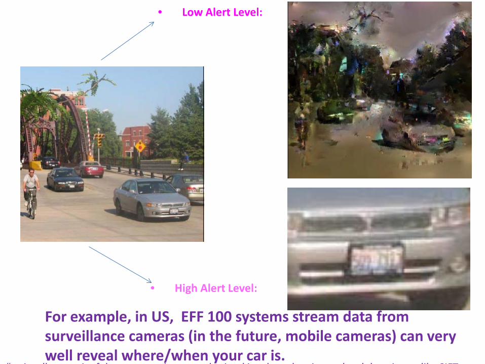
• Low Alert Level:

• High Alert Level:

For example, in US, EFF 100 systems stream data from surveillance cameras (in the future, mobile cameras) can very well reveal where/when your car is.

Discriminant Component Analysis (DCA) offers a compression scheme to enhance privacy protection in contextual and collaborative learning environment. The DCA has

(a) its classification goal characterized by the discriminant distance and

(b) its privacy components controlled by a ridge parameter. Therefore, DCA is a promising algorithmic tool for CP.

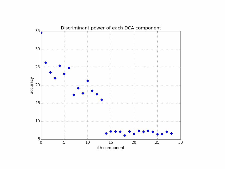
Discriminant Component Analysis (DCA)

ρ’ = 0.00001≈0

Rank Order SU and NU Rank Order SP and NP

This is not good enough as we want to

Noise-Subspace Eigenfaces

ρ’ = 0.00001

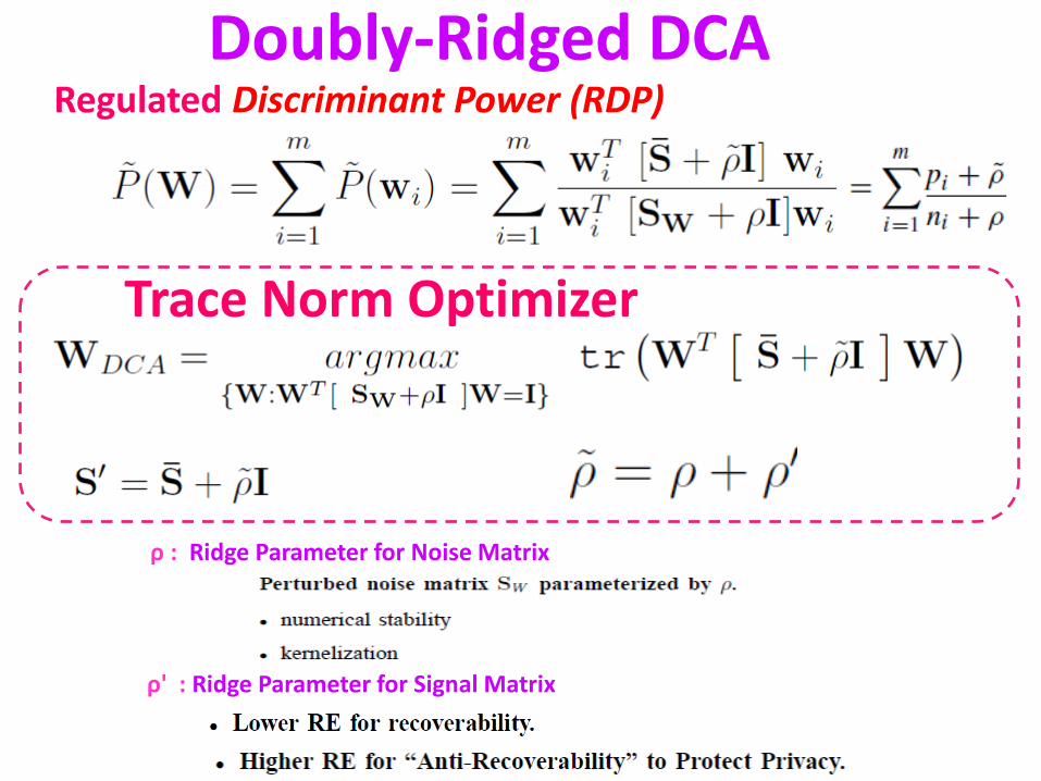
Doubly-Ridged DCA

ρ : Ridge Parameter for Noise Matrix

ρ' : Ridge Parameter for Signal Matrix

Trace Norm Optimizer

Regulated Discriminant Power (RDP)

Algorithm: DCA Learning Model • Compute the Discriminant Matrix:

under the canonical normality that

• Perform Eigenvalue Decomposition:

• The optimal DCA projection matrix is:

maximizing RE for anti-reconstruction

maximizing component power for utility maximizatio

Principal Eigenvalues for the Private Subspace:

Minor Eigenvalues for the Privatized Subspace:

Dual Roles of P-DCA Eigenvalues Simultaneously rank-order two subspaces:

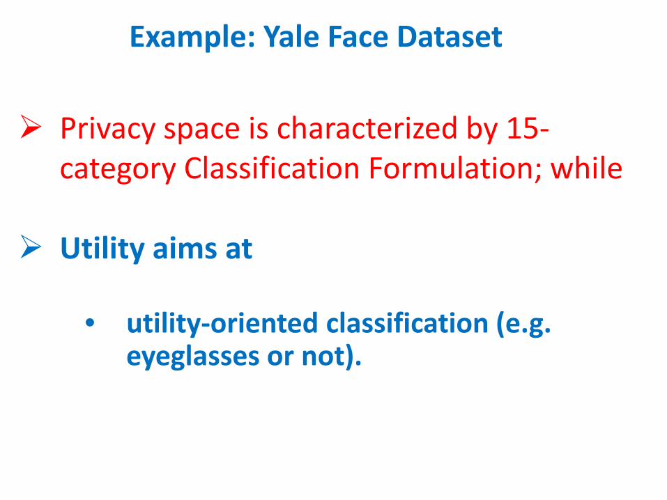
Privacy space is characterized by 15-category Classification Formulation; while

Utility aims at

• utility-oriented classification (e.g.

eyeglasses or not).

Example: Yale Face Dataset

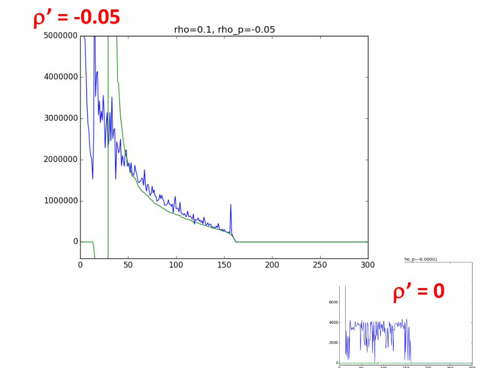
ρ’ = -0.05

ρ’ = 0

Private Eigenfaces

PU (Privatized/Utilizable) Eigenfaces

ρ’ = -0.05

w/o rank ordering

w. rank ordering

ρ’ = -0.05

ρ’ = +0.00001

<

< <

<

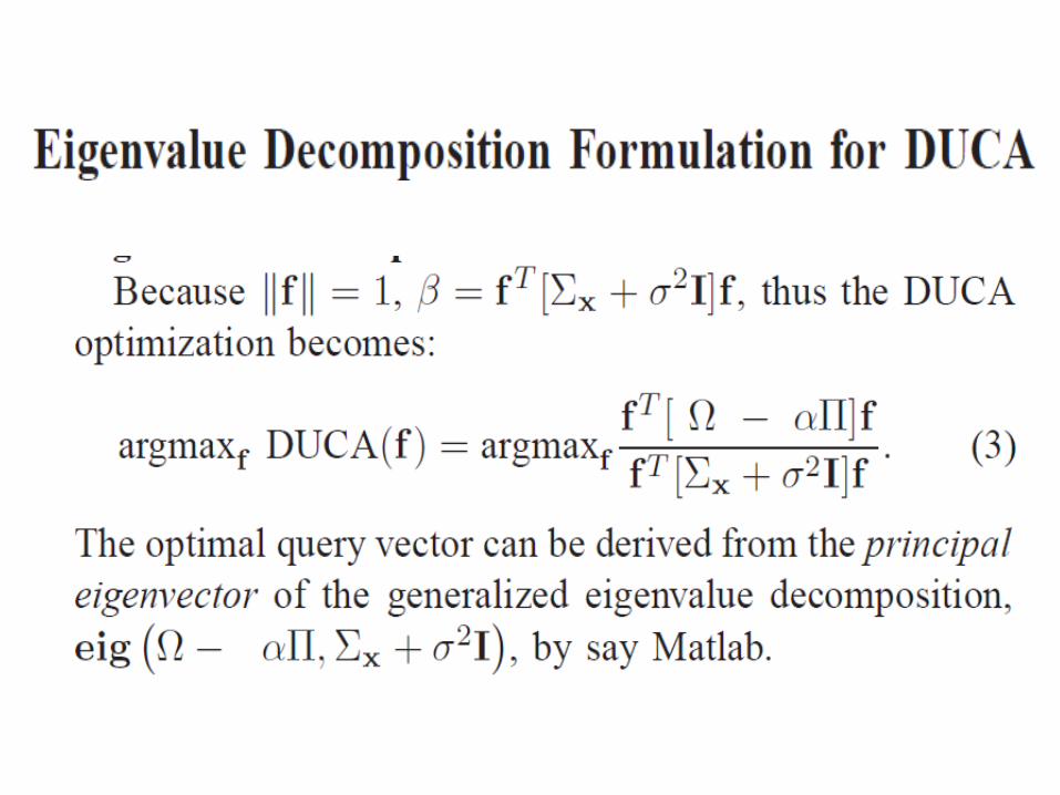
We shall explore joint optimization over three design spaces: (a) Feature Space, (b) Classification Space, and (c) Privacy Space. This prompts a new paradigm called DUCA to explore information systems which simultaneously perform Utility Space Maximization: deliver intended data mining, classification, and learning tasks.


iv. Differential Utility/Cost Advantage (DUCA)

DUCA ≠

DCA

PCA

DUCA

Our (CP) approach involves joint optimization over three design spaces: (i) Feature Space (ii) Utility Subspace; and (iii) Cost Subspace (i.e. Privacy Subspace).

Entropy and Venn Diagram

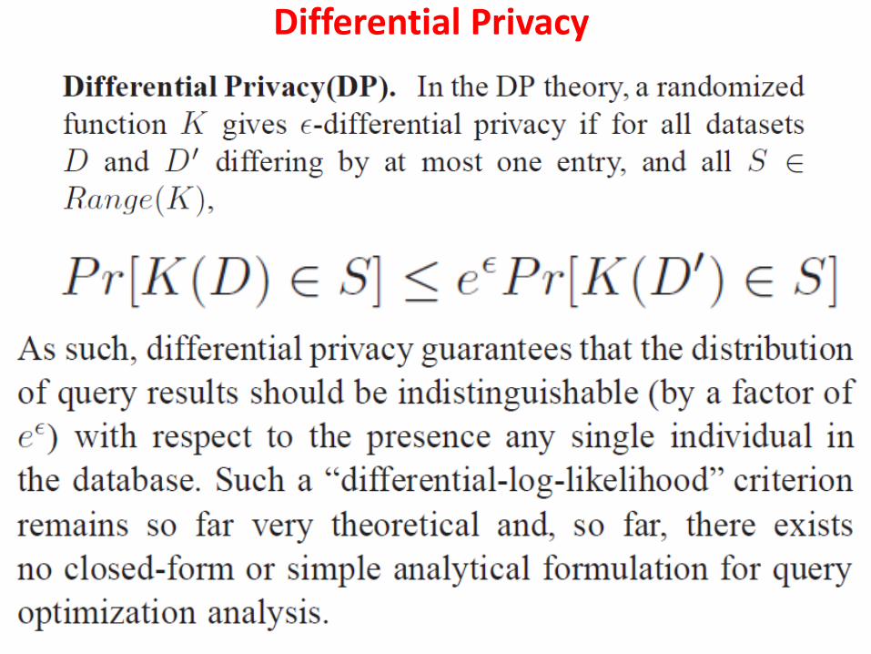
Differential Privacy

CP enables the data user to “encrypt” message using privacy-information-lossy transformation, e.g.

• Dimension reduction (Subspace) • Feature selection

hence • preserving data owner's privacy while • retaining the capability in facilitating

the intended classification purpose.

Compressive Privacy (CP)

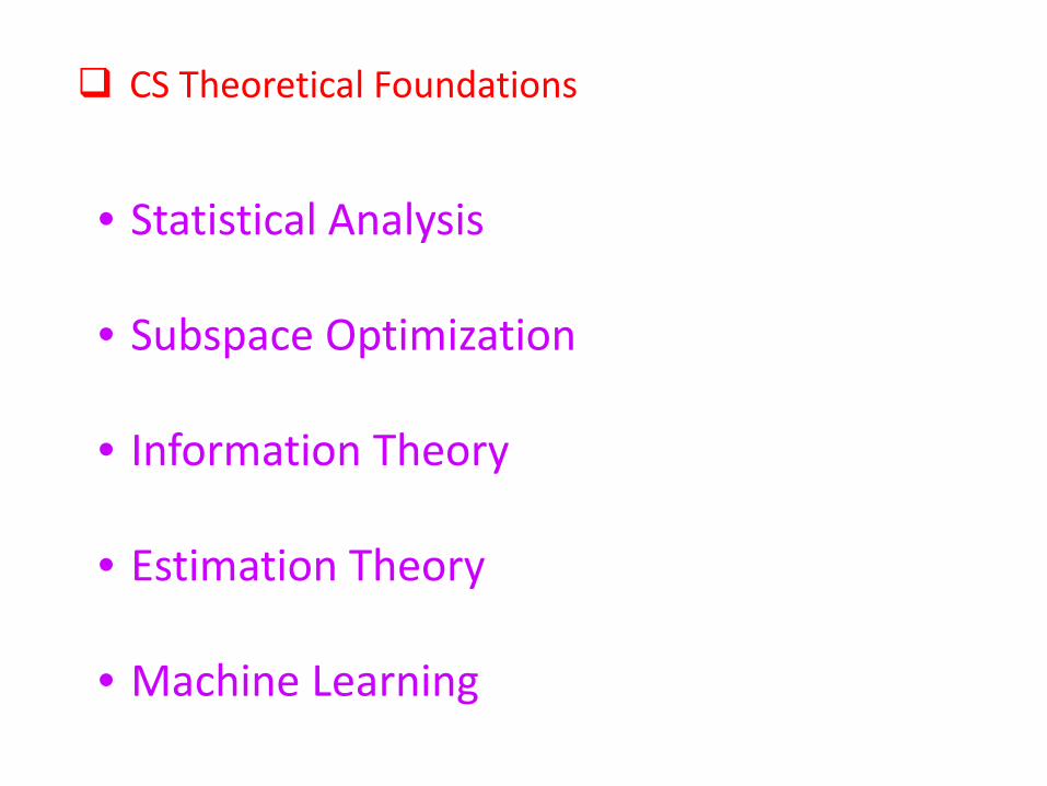
CS Theoretical Foundations

• Statistical Analysis • Subspace Optimization

• Information Theory

• Estimation Theory

• Machine Learning

Entropy and Covariance Matrix

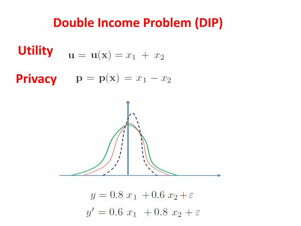
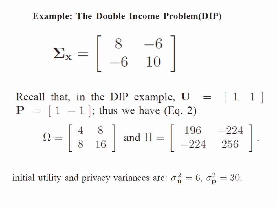
Double Income Problem (DIP)

Privacy

Utility

Compressive Privacy

Estimation Theory and Compressive Privacy

argmin ( || fT - y || 2 + || ||2 )

Gauss-Markov (Statistical Estimation) Theorem

Machine Learning and Compressive Privacy

For CP problems, there are two types of the teacher values in the dataset: one for the utility labels and one for privacy labels. It implies that there are two types of between-class scatter matrices, denoted by

for the utility labels

and

for the privacy labels.

DUCA for Supervised Machine Learning

Generalized Eigenvalue Problem Again, the optimal queries can be directly derived from the principal eigenvectors of

where L and C denote the numbers of utility and privacy labels.

Note that there are only L+C-2 meaningful eigenvectors, because

DUCA is only a generalization of its predecessor, called DCA, designed for the utility-only machine learning applications.

𝑠𝑛

𝑠 + 𝑛𝑛

𝑠

𝑠 + 𝑛

Naturally, just like DCA, there are ways for DUCA to extract additional meaningful queries.

argmax argmax argmax

where ``H/M/L" denotes the three (High/Middle/Low) utility classes (i.e. family income) and ``+/-" denotes the two privacy classes (i.e. who-earns-more between the couple).

with the utility/ privacy class labels

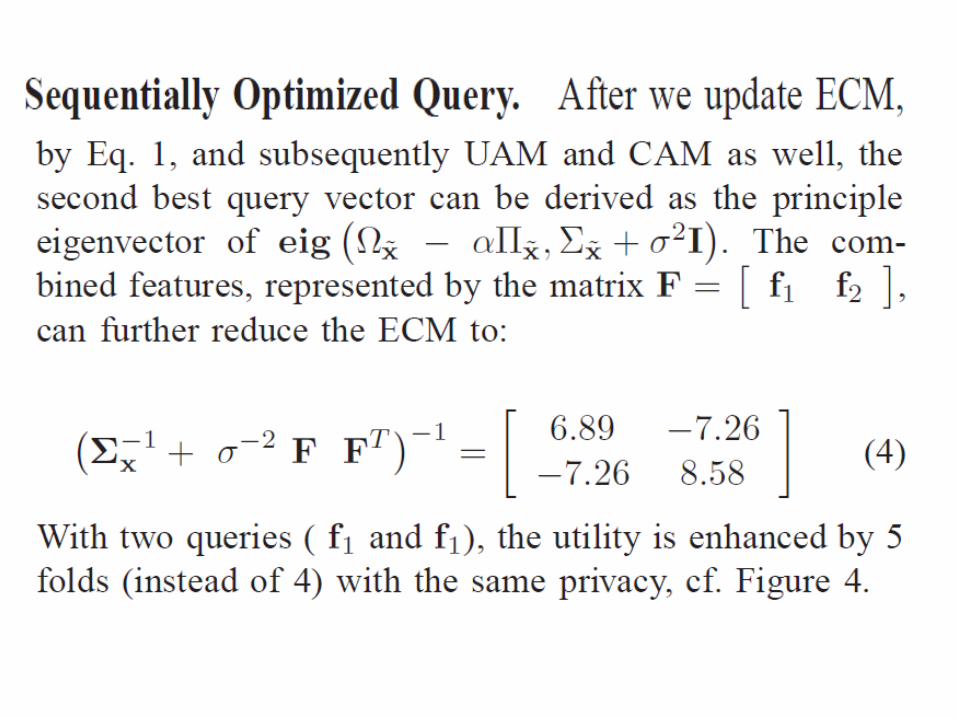
UAM and CAM can be learned from the given dataset and their respective class labels.

𝑓1 =-0.14-0.87-0.17-0.44

𝑓2 =-0.002-0.110.680.72

Parallel Extraction of Multiple Queries: Thereafter, the two principle eigenvectors of the generalized eigenvectors of can be computed as

The two-dimensional visualization of the DUCA-CP subspace, in which the family income classes (H/M/L) are highly separable but not so for the income disparity categories (+/-). For example, the query here obviously belongs to the middle-class (utility) but its disparity (privacy) remains unknown, i.e. protected.

Four Categories of PPUM Formulations

• CUCP classification formulation for both utility and privacy;

• EUEP estimation formulation for both utility and privacy;

• EUCP estimation for utility but classification for privacy;

• CUEP classification for utility but estimation for privacy.

C: classification E: estimation

U: Utility CU EU P: Privacy CP EP

If the privacy function is prescribed by the matrix P, just replace by .

If the utility function is prescribed by the matrix P, just replace by .

If the privacy function is prescribed by the matrix P, we have the following adjustments:

Three reconstruction images are based on 399 selected FFT components by different filters: (a) rectangular window (no-learning); (b) unsupervised filtering based on the component's variances; and (c) supervised filtering based on component's FDRs. (Courtesy from A. Filipowicz.)

(b) 73.9% (a) 73% (c) 73%

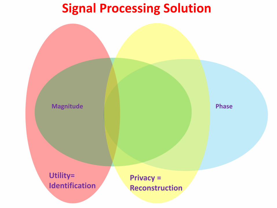
Utility= Identification

Phase Magnitude

Privacy = Reconstruction

Signal Processing Solution

Full Dimension Olivetti Original

Reconstruction

Phase Information Proves Vital for Reconstruction, it has little, if not negative, impact on Classification.

Reconstruction

w. phase

w/o phase

(0.97)

(0.9725)

Big data analysis usually involves nonlinear data analysis and the two most promising approaches for which kernel learning machine (KLM) and deep learning machine (DLM). The safest possible protection is to withhold the privy data from sharing in the first place. This schema, however, presents a formidable challenge in developing a machine learning tool for incomplete data analysis (IDA). Fortunately, KLM can naturally be extended to all types of nonvectorial data analysis including IDA. Moreover, KLM can facilitate: Intrinsic space and privacy: Reduce the number of training vectors need to be stored in the cloud (SVM) or even make it unnecessary to share any training data via the intrinsic kernel approach. Auto-encoder for privacy: Compare two nonlinear Auto-Encoders (KLM and DLM) for data minimizer. Kernel learning machine for privacy: For example, partially-specified feature vectors can be pairwise correlated to yield a similarity or kernel function for kernel learning machine (KLM). Thereafter, SVM or KRR supervised learning classifiers may be trained and deployed for prediction applications.

Machine Learning for Compressive Privacy v. Nonlinear and Kernel Learning Machines

The key of success lies in an effective representation of the objects by a much expanded vector space:

• Kernel Vector Space


Feature Engineering


The feature engineering step is very laborious. Training data (e.g. human-labeled images) are used, often by trial-and-error, to learn features representative of the target (e.g. cars) .

No learning at all in the feature engineering step.

• Multilayers of Hidden Nodes in Deep Learning

Kernel learning (aka shallow learning) vs. the dull nature of deep learning!!

Big data analysis usually involves nonlinear data analysis, for which kernel machine learning (KML) and deep learning (DML) represent the two most promising approaches. KML and DML differs in the fact that KML is based on pairwise quantification of any pair of targeted objects while DML extract feature vector for each of the targeted objects, using a cascade of feature extraction layers. In this sense, the two learning approaches complement each other very well. This points to a potentially integration of both KML and DML technologies.

Deep back-propagation and kernel learning algorithms

Nonlinear Supervised Learning Machine

Basic Learning Module in BP

Back Propagation (BP) Neural Network

BP was the key Supervised Learning Networks in 80’s.

Deep Learning Networks or Deep Learning Machines

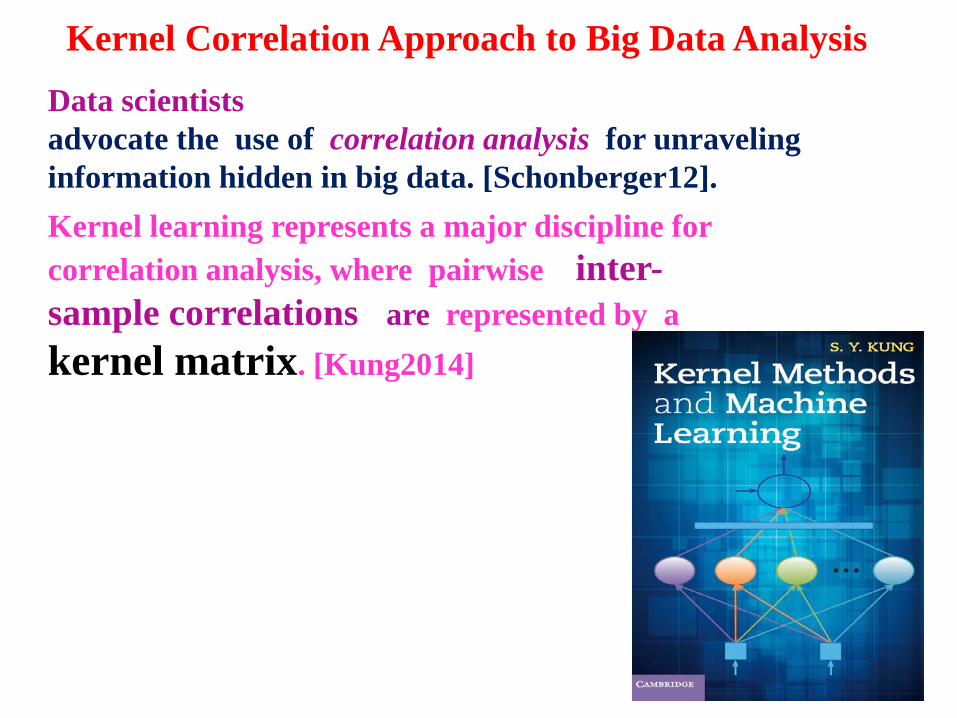
Data scientists advocate the use of correlation analysis for unraveling information hidden in big data. [Schonberger12].

Kernel Correlation Approach to Big Data Analysis

Kernel learning represents a major discipline for correlation analysis, where pairwise inter-sample correlations are represented by a kernel matrix. [Kung2014]

• Curse of Dimensionality (Volume)

• Curse of Large Data Size (Velocity) • Curse of High Feature Dimensionality

Data

Matrix

Kernel Matrix

Kernel Approach?

𝑴

𝑵

𝑴

𝑴

𝑵

𝑵

• Correlation Analysis (Statistical Perspective)

• Algorithmic Analysis (Algebraic and Optimization Principles)

Kernel vs. BDA

Covariance Matrix

Kernel Approach to (Big) Data Analysis

The dimension J,

Training-data-independent intrinsic feature vectors

𝜙 (𝑥)

𝑥

→

LSP→

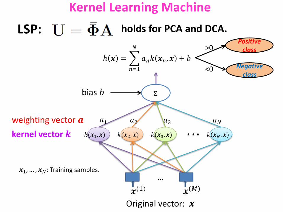
Original vector: 𝒙

𝑘(𝒙1, 𝒙)

𝒙(1) 𝒙(𝑀)

Σ

ℎ 𝒙 = � 𝑎𝑛𝑘 𝒙𝑛, 𝒙 + 𝑏𝑁

𝑛=1

𝑎1 𝑎2 𝑎3 𝑎𝑁

𝑘(𝒙2, 𝒙) 𝑘(𝒙3, 𝒙) 𝑘(𝒙𝑁 , 𝒙) kernel vector 𝒌 weighting vector 𝒂

…

Positive class

Negative class

>0

<0

bias 𝑏

𝒙1, … , 𝒙𝑁: Training samples.

Kernel Learning Machine

LSP: holds for PCA and DCA.

𝑆(𝒙1, 𝒙1) 𝑆(𝒙1, 𝒙2)𝑆(𝒙2, 𝒙1) 𝑆(𝒙2, 𝒙2) ⋯ 𝑆(𝒙1, 𝒙𝑁)

𝑆(𝒙1, 𝒙2)⋮ ⋱ ⋮

𝑆(𝒙𝑁, 𝒙1) 𝑆(𝒙𝑁, 𝒙1) ⋯ 𝑆(𝒙𝑁, 𝒙𝑁)

imputation

non-

vect

ors

The data is individually quantified!!

Vectorization vs. Pairwise Kernel

K(•,•)

non-

vect

ors

Non-vectorial data are pairwise quantified into similarity matrix.

= K

deep learning

kernelization

Vectorization

Kernel trick [Aizerman’64]

Linear, Nonlinear, & Non-Vectorial Kernel Machines

linear

nonlinear

Nonlinear Kernel Machines for vector data:

𝑆(𝒙1, 𝒙1) 𝑆(𝒙1, 𝒙2)𝑆(𝒙2, 𝒙1) 𝑆(𝒙2, 𝒙2) ⋯ 𝑆(𝒙1, 𝒙𝑁)

𝑆(𝒙1, 𝒙2)⋮ ⋱ ⋮

𝑆(𝒙𝑁 , 𝒙1) 𝑆(𝒙𝑁 , 𝒙1) ⋯ 𝑆(𝒙𝑁 , 𝒙𝑁)

Non-Vectorial Kernel Machines

Non-vectorial data are pairwise quantified, instead of individually quantified!!

Vector and non-vector correlation analysis

PSI-BLAST

Adjacency Matrix

? Partial Correlation

Pairwise Quantified Kernel Matrix


The “partial correlation” of the joint features points to the same (type of) animal.

( )xyxy

xy

II

I

yx

yx,yx,K ≡

xyIjoint

features

The objective of machine learning is often an effective classification of objects, new and unseen before.

• Kernel Ridge Regression (KRR): • tuning parameter (ρ)

• Support Vector Machine (SVM): • tuning parameter (C)

• Ridge-SVM • more tuning parameters


Feature Engineering


Turing Machines ⇒ Tuning Machines

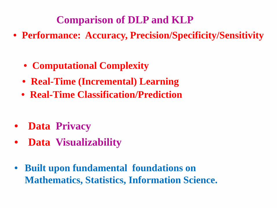
• Data Privacy

Comparison of DLP and KLP

• Built upon fundamental foundations on Mathematics, Statistics, Information Science.

• Data Visualizability

• Performance: Accuracy, Precision/Specificity/Sensitivity

• Real-Time (Incremental) Learning • Real-Time Classification/Prediction

• Computational Complexity

SVM/KRR

nonvectorial data

vectorial data

Deep

Learning

Features

Kernel Features

(No Learning)

PCA

DCA

KPCA

KDCA

Feature

Selection

Pairwise

Quantified

System Integration

Original vector: 𝒙 𝑥1 𝑥𝑀

Σ

A New Hope → Intrinsic Space O(J)

intrinsic vector 𝒛 𝑧1(𝒙) 𝑧2(𝒙) 𝑧3(𝒙) 𝑧𝐽(𝒙)

decision vector 𝒖

threshold: 𝑏 Σ

ℎ� 𝒙 = � 𝑢𝑗𝑧𝑗(𝒙)𝐽

𝑗=1

+ 𝑏

𝑢1 𝑢2 𝑢3 𝑢𝐽

Finite Order means that classification complexity can be independent of N.

Kernelized DCA (KDCA)

Visualization via Linear DCA


Derivation of KDCA in Intrinsic Space Data Matrix in Intrinsic Space

Projection Matrix in Intrinsic Space

KDCA representation in Intrinsic Space

Within-Class Scatter Matrix in Intrinsic Space

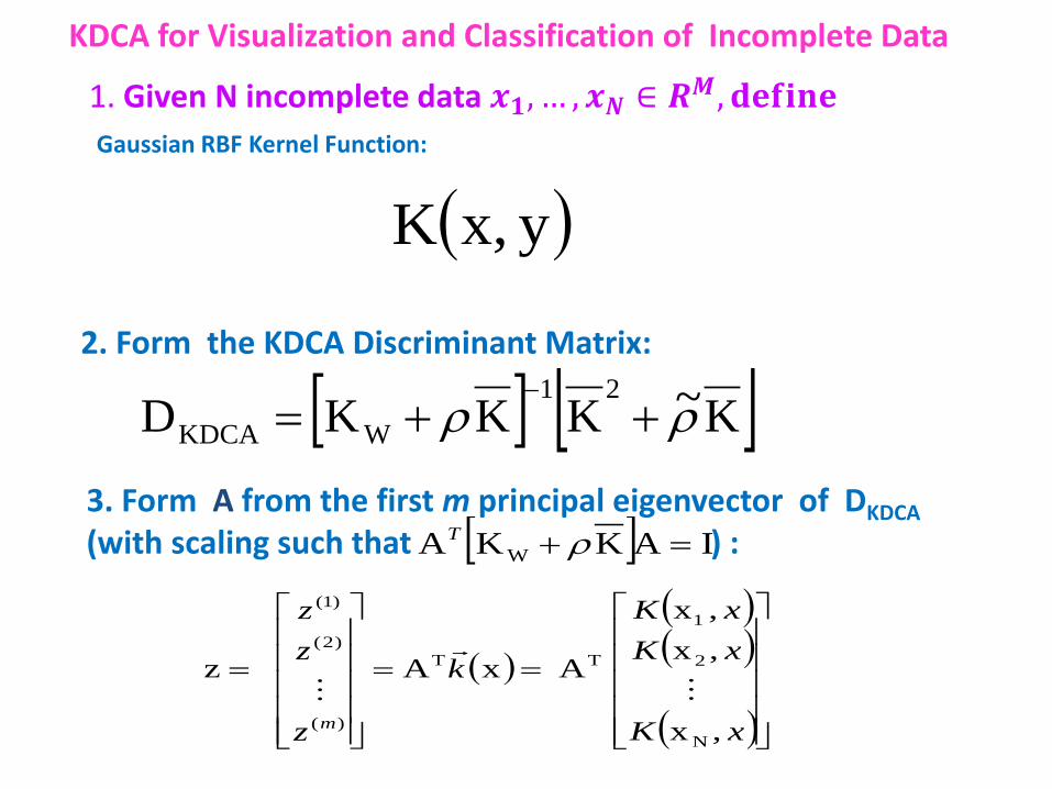
KDCA for Visualization and Classification of Incomplete Data

1. Given N incomplete data 𝒙𝟏, … , 𝒙𝑵 ∈ 𝑹𝑴, 𝐝𝐝𝐝𝐝𝐝𝐝

[ ] [ ]K~KKKD21

WKDCA ρρ ++=−

( )

( )( )

( )

==

=

xK

xKxK

k

z

zz

m ,x

,x,x

A xA z

N

2

1

TT

)(

)2(

)1(

3. Form A from the first m principal eigenvector of DKDCA (with scaling such that ) :

2. Form the KDCA Discriminant Matrix:

[ ] IAKKA W =+ ρT

Gaussian RBF Kernel Function:

( )yx,K

Visualization via (RBF) KDCA

Original Masked Data

How do we cope with masked data?

…not in vector form.

Pairwise Quantified Kernel Matrix

? Partial Correlation


The “partial correlation” of the joint features points to the same (type of) animal.

( )xyxy

xy

II

I

yx

yx,yx,K ≡

xyIjoint

features

KDCA for Visualization and Classification of Incomplete Data

1. Given N incomplete data 𝒙𝟏, … , 𝒙𝑵 ∈ 𝑹𝑴, 𝐝𝐝𝐝𝐝𝐝𝐝

[ ] [ ]K~KKKD21

WKDCA ρρ ++=−

( )

( )( )

( )

==

=

xK

xKxK

k

z

zz

m ,x

,x,x

A xA z

N

2

1

TT

)(

)2(

)1(

3. Form A from the first m principal eigenvector of DKDCA (with scaling such that ) :

2. Form the KDCA Discriminant Matrix:

[ ] IAKKA W =+ ρT

Partial Correlation Kernel: This image cannot currently be displayed.

No dim reduction

Missing Ratio

KAIDA (SVM): Masking Only 0.4% Loss

Non-Imputed PC Kernel

Imputed RBF Kernel

accu

racy

missing ratio

0% 10% 25% 50% 75%

accu

racy

100%

98%

96%

94%

92%

90%

88%

86%

missing ratio

Original

Best of both worlds: Compression and Masking

DCA is good for compressed data.

Compressed Data

… in vector form.

Masked Data

How do we cope with masked and dimension-reduced data?

…not in vector form.

Kernel DCA (KDCA)

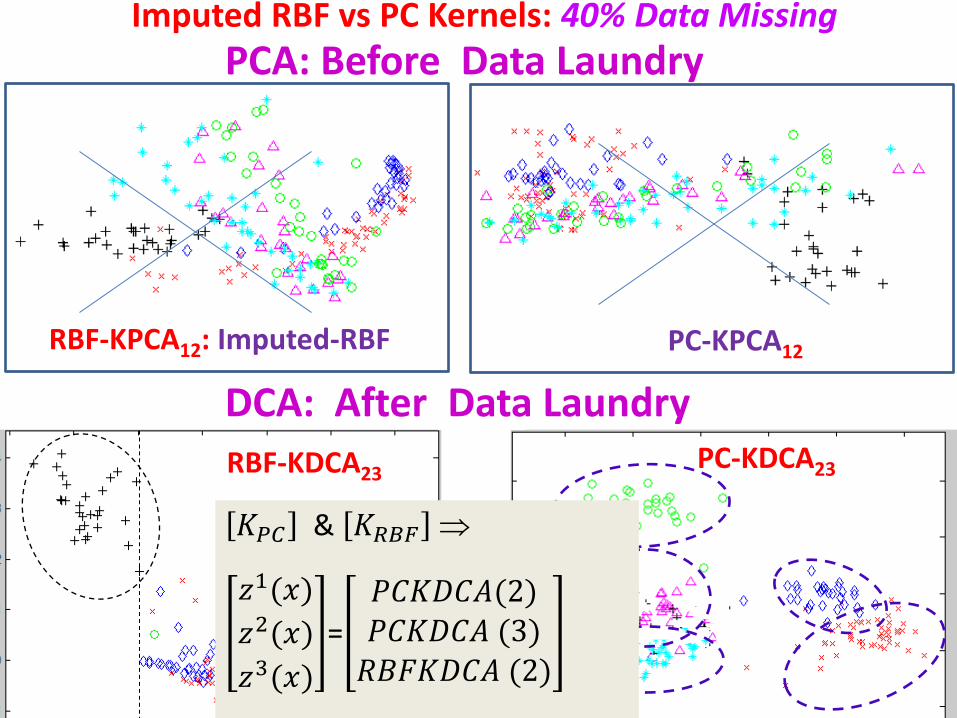
Imputed RBF vs PC Kernels: 40% Data Missing

RBF-KDCA23

DMPC KDCA: Imputed RBF

PC-KDCA23

𝐾𝑃𝑃 & 𝐾𝑅𝑅𝑅 ⇒

𝑧1(𝑥)𝑧2(𝑥)𝑧3(𝑥)

=𝑃𝑃𝐾𝑃𝑃𝑃(2)𝑃𝑃𝐾𝑃𝑃𝑃 (3)

𝑅𝑅𝑅𝐾𝑃𝑃𝑃 (2)

DCA: After Data Laundry

PCA: Before Data Laundry

RBF-KPCA12: Imputed-RBF PC-KPCA12

• DUCA-CP for Joint optimization

Some Parting Thoughts on Internet Privacy

• Needs good foundations on Mathematics, Statistics, Information Science.

• Thank you and Question?

• DCA/KDCA: Shields for Privacy Protection

kung slides - cs.ioc.ee

Documents